Fourth-order problems with nonlinear boundary conditions

Journal of Computational and Applied Mathematics 174 (2005) 315–327

www.elsevier.com/locate/cam

Fourth-order problems with nonlinear boundary conditions�

Daniel Francoa,∗, Donal O’Reganb, Juan Perána

aDepartamento de Matemática Aplicada, Universidad Nacional de Educación a Distancia,Apartado de Correos 60149, Madrid 28080, Spain

bDepartment of Mathematics, National University of Ireland, Galway, Ireland

Received 4 November 2003; received in revised form 20 April 2004

Abstract

We develop a new method of lower and upper solutions for a fourth-order nonlinear boundary value problem wherethe differential equation has dependence on all lower-order derivatives. Our boundary conditions are nonlinear. Wewill assume the functions that define the nonlinear boundary conditions are either monotone or nonmonotone. Asa result we obtain existence principles which improve recent results in the literature.© 2004 Elsevier B.V. All rights reserved.

Keywords:Fourth-order nonlinear boundary value problems; Lower and upper solutions; Beam equation

1. Introduction

Several papers have appeared which use the lower and upper solution method and which study theexistence of solutions for fourth-order (or even 2mth-order) problems. Some of these papers have nononlinear dependence on any of the lower-order derivatives (see[3] and references therein), others dealwith differential equations that depend only on even-order derivatives (see[2,3,6,15]), and a few papersstudy problems with nonlinear dependence on all the lower-order derivatives (see[7]).

Recently, several papers have appeared which use the lower and upper solution method and study theexistence of solutions for fourth-order (or even 2mth-order) problems. However these papers have no

� The first author was supported in part by Ministerio de Ciencia y Tecnología (Spain) and FEDER, project BFM2001-3884-C02-01.∗ Corresponding author. Tel.: +34-913988134; fax: +34-913986012.

E-mail address:[email protected](D. Franco).

0377-0427/$ - see front matter © 2004 Elsevier B.V. All rights reserved.doi:10.1016/j.cam.2004.04.013

316 D. Franco et al. / Journal of Computational and Applied Mathematics 174 (2005) 315–327

nonlinear dependence on any of the lower-order derivatives or only on even-order derivatives. We referthe reader to[2,3,6,7,15]for a complete list of references in the subject.

Most of the papers considering fourth-order problems deal with linear boundary conditions. In thelast few years several authors consider nonlinear boundary conditions that permit even different types oflinear boundary conditions together. In a recent paper Ehme et al.[7] considered

k1(u)= 0, l1(u)= 0,k2(u)= 0, l1(u)= 0,

(1)

whereu = (u(0), u(1), u′(0), u′(1), u′′(0), u′′(1)). Notice that for example, if we letk1(u) = u(0),l1(u) = u(1), k2(u) = u′′(0), l1(u) = u′′(1) we obtain Lidstone boundary conditions. A common hy-pothesis in papers related to problems with nonlinear boundary conditions is the existence of some fixedmonotone behavior in each variable of the functions which define the nonlinear boundary conditions.We refer the reader to[4,8–11,13,16,18]for papers assuming such conditions and dealing with ordinarydifferential equations.

In [7] the authors show the applicability of the lower and upper solution method to the problem formedby the differential equation,

u(iv)(t)= f (t, u(t), u′(t), u′′(t), u′′′(t)), t ∈ I = [0,1] (2)

and the boundary conditions (1). In[7] because of the dependence on odd derivatives, the authors employthe Kamke existence of solutions of initial value problems theorem[12].

One of the aims of this paper is to generalize the results presented by Ehme et al. In order to do so and inaddition to consider more general nonlinear boundary conditions than the ones considered in[7] we shalluse a different truncated problem and we shall not need to employ the Kamke existence of solutions ofinitial value problems theorem. In Section 2, we shall consider nonlinear boundary conditions satisfyingmore general monotone conditions than in[7]. In Section 3, we shall show how these conditions can beremoved and we shall present an example not covered by results in the literature to date. The last sectionis devoted to the study of nonlinear boundary conditions that include the periodic and anti-periodicproblems.

Several models can be studied with our results. Consider a model of an elastic strut supported byan elastic foundation; a model of patter formation in polymeric materials under tension; a model ofsuspension bridges. Both these examples use the equation[5,17],

u(iv) + pu′′ + F ′(u)= 0.

In this paper we shall consider

u(iv)(t)= f (t, u(t), u′(t), u′′(t), u′′′(t)), t ∈ I = [0,1], (3)

satisfying the nonlinear boundary conditions

g1(u)= 0, h1(u)= 0,g2(u)= 0, h2(u)= 0, (4)

with f : I × R4 → R, g1, g2 : R6 → R, h1, h2 : R8 → R continuous functions andu andu standing for

u= (u(0), u(1), u′(0), u′(1), u′′(0), u′′(1)),u= (u(0), u(1), u′(0), u′(1), u′′(0), u′′(1), u′′′(0), u′′′(1)).

D. Franco et al. / Journal of Computational and Applied Mathematics 174 (2005) 315–327 317

To conclude the Introduction we present some basic definitions, notation and the main tool that weshall employ in the proof of our result.

As usual inC(I)we shall consider the norm|u|0 =supt∈I |u(t)| and the partial order given by the coneof positive functions. Also, foru, v ∈ C(I), we shall write

[u, v] = {w ∈ C(I) : u(t)�w(t)�v(t), t ∈ I }.We next introduce the Nagumo condition that we use.

Definition 1. Let �, � ∈ C4(I ) such that��� and�′′��′′. We say thatf satisfies a Nagumo conditionrelative to�, � if for

r0 = max{|�′′(0)− �′′(1)|, |�′′(1)− �′′(0)|}there exists a constantD such that

D>max{r0, |�′′′|0, |�′′′|0

}

and a continuous function� : [0,∞) → (0,∞) such that

|f (t, x, y, z, w)|��(|w|), t ∈ I, x ∈ [�(t), �(t)], y ∈ [−C,C],z ∈ [�′′(t), �′′(t)], w ∈ R,

and ∫ D

r0

1

�(s)ds >1, (5)

here

C = 2 max{|�′|0, |�′|0} + max{|�(0)− �(1)|, |�(1)− �(0)|}. (6)

Definition 2. We say that the mapL : X → Y between two metric spaces is compact ifL(X) is acompact subset ofY.

Theorem 1. [Schauder’s fixed point theorem, Agarwal et al. [1]].Let K be a convex subset of a normedlinear space E. Each continuous, compact mapL : K → K has a fixed point.

2. Monotone boundary conditions

In order to simplify the notation, for each� ∈ C3(I ) we define the following functions:

g�1(x, y, z, w) :=g1(�(0), x, �

′(0), y, z, w), x, y, z, w ∈ R,

g�2(x, y, z, w) :=g2(x, �(1), y, �

′(1), z, w), x, y, z, w ∈ R,

h�1(x, y, z, w, v, u) :=h1(x, y, z, w, �

′′(0), v, �′′′(0), u), x, y, z, w, v, u ∈ R,

h�2(x, y, z, w, v, u):=h2(x, y, z, w, v, �

′′(1), u, �′′′(1)), x, y, z, w, v, u ∈ R.

318 D. Franco et al. / Journal of Computational and Applied Mathematics 174 (2005) 315–327

Our next step will be the introduction of a new definition of lower and upper solutions for problems(3) and (4).

Definition 3. We say that�, � ∈ C4(I ) are coupled lower and upper solutions for the problems (3) and(4) if ���, �′′��′′,

�(iv)(t)�f (t, �(t),−C, �′′(t), �′′′(t)) for t ∈ I,�(iv)(t)�f (t, �(t), C, �′′(t), �′′′(t)) for t ∈ I (7)

and

min(x,y,z,w)∈A1

{g�1(x, y, z, w)}�0� max

(x,y,z,w)∈A1{g�

1(x, y, z, w)} (8)

with A1 = {(x, y, z, w) : x ∈ {�(1), �(1)}, y ∈ {−C,C}, z ∈ {�′′(0), �′′(0)}, w ∈ {�′′(1), �′′(1)}},min

(x,y,z,w)∈A2{g�

2(x, y, z, w)}�0� max(x,y,z,w)∈A2

{g�2(x, y, z, w)} (9)

with A2 = {(x, y, z, w) : x ∈ {�(0), �(0)}, y ∈ {−C,C}, z ∈ {�′′(0), �′′(0)}, w ∈ {�′′(1), �′′(1)}},min

(x,y,z,w,v,u)∈B1{h�

1(x, y, z, w, v, u)}�0� max(x,y,z,w,v,u)∈B1

{h�1(x, y, z, w, v, u)} (10)

with B1 = {(x, y, z, w, v, u) : x ∈ {�(0), �(0)}, y ∈ {�(1), �(1)}, z, w ∈ {−C,C}, v ∈ {�′′(1), �′′(1)},u ∈ {−D,D}},

min(x,y,z,w,v,u)∈B2

{h�2(x, y, z, w, v, u)}�0� max

(x,y,z,w,v,u)∈B2{h�

2(x, y, z, w, v, u)} (11)

with B2 = {(x, y, z, w, v, u) : x ∈ {�(0), �(0)}, y ∈ {�(1), �(1)}, z, w ∈ {−C,C}, v ∈ {�′′(0),�′′(0)}, u ∈ {−D,D}}; hereC andD were introduced in Definition 1.

It is worth noting that this definition generalizes the concepts employed in the literature for linearand nonlinear boundary conditions. For example, in[7, Definition 2.1] the concept of strong uppersolution–lower solution pair for (1) and (2) is considered i.e. (7) is assumed and (8)–(11) are replaced byinequalities:

k1(�)�0�k1(�), l1(�)�0� l1(�),k2(�)�0�k2(�), l2(�)�0� l2(�)

with u = (�(0), �(1),−C,−C, �′′(0), �′′(1)) and � = (�(0), �(1), C,C, �′′(0), �′′(1)). Now, with themonotonicity hypotheses imposed in[7] it is easy to see that if�, � is a strong upper solution–lowersolution pair then they are coupled lower and upper solutions.

On the other hand, we also note that if there exists a dependence onu′ in the nonlinearityf it isimpossible to define a lower and upper solution independently. However, iff has no dependence onu′ itmay be possible to define a lower and upper solution independently. For example, if we consider Lidstonedata then conditions (8)–(11) are the classical conditions,

�(0)�0, �′′(0)�0,�(1)�0, �′′(1)�0

and�(0)�0, �′′(0)�0,�(1)�0, �′′(1)�0

and we can define a lower and upper solution independently.

D. Franco et al. / Journal of Computational and Applied Mathematics 174 (2005) 315–327 319

The main result in this section is the following.

Theorem 2. Suppose f satisfies a Nagumo condition relative to�, �. Also assume that�, � are coupledlower and upper solutions for problems(3) and(4) and the following conditions hold:

(H1) the function f is nondecreasing in the second and third variable;(H2) the functionsg1 and g2 are nondecreasing and nonincreasing in the third and fourth variable,

respectively, and the functionsh1 andh2 are nondecreasing and nonincreasing in the seventh andeighth variable, respectively;

(H3) the functionsg�i , g

�i ,h�

i ,h�i aremonotone(either nonincreasing or nondecreasing) in each variable

(i = 1,2).Then there exists at least one solution u of(3) and(4) such thatu ∈ [�, �], u′ ∈ [−C,C], u′′ ∈ [�′′, �′′]andu′′′ ∈ [−D,D].Proof. In order to define a suitable modified problem we introduce the functions

m(t, x)= max{�(t),min{x, �(t)}}, n(t, x)= max{−C,min{x, C}}and

p(t, x)= max{�′′(t),min{x, �′′(t)}}, q(t, x)= max{−D,min{x,D}}.We consider the modified problem,

u(iv)(t)= F ∗(t, u(t), u′(t), u′′(t), u′′′(t)), t ∈ I,u(0)= g∗

1(u), u′′(0)= h∗1(u),

u(1)= g∗2(u), u′′(1)= h∗

2(u) (12)

with

F ∗(t, x, y, z, w)= f (t,m(t, x), n(t, y), p(t, z), q(t, w))+ z− p(t, z)

1 + |z− p(t, z)| ,

g∗1(u)=m(0, u(0)+ g1(u)), h∗

1(u)= p(0, u′′(0)+ h1(u)),

g∗2(u)=m(1, u(1)+ g2(u)), h∗

2(u)= p(1, u′′(1)+ h2(u)).

We shall divide the proof into six steps:Step1: Problem (12) has at least a solution.It is well known[19] that solving (12) is equivalent to finding a fixed point of the operator

N : C3(I ) → C3(I )

defined by

Nu(t)=g∗2(u)t + g∗

1(u)(1 − t)+∫ 1

0G(t, s)[h∗

2(u)s + h∗1(u)(1 − s)] ds

+∫ 1

0H(t, s)F ∗(s, u(s), u′(s), u′′(s), u′′′(s))ds,

320 D. Franco et al. / Journal of Computational and Applied Mathematics 174 (2005) 315–327

where

G(t, s)={t (s − 1), 0� t < s�1,s(t − 1), 0�s < t�1

and H(t, s)=∫ 1

0G(t, r)G(r, s)dr.

Let us consider inC3(I ) the norm‖ u ‖ = max{|u|0, |u′|0, |u′′|0, |u′′′|0}.Using the continuity of the functions that define our problem and the definitions of the functions of the

modified problem together with the Ascoli–Arzelá theorem one can easily see thatN is continuous andcompact. Thus Schauder’s fixed point theorem guarantees the existence of at least a fixed point.Step2: If u is a solution of (12) thenu′′ ∈ [�′′, �′′].By the definition ofh∗

1 andh∗2 (notep(t, x) ∈ [�′′(t), �′′(t)] for t ∈ I andx ∈ R) we see thatu′′(0) ∈

[�′′(0), �′′(0)] andu′′(1) ∈ [�′′(1), �′′(1)].Therefore, it remains to show that�′′(t)�u′′(t)��′′(t) for t ∈ (0,1). Let v = u− � and suppose that

there existst0 ∈ (0,1) such thatv′′(t0)<0. Then there existr, s ∈ (0,1) such thatr < s, v′′′(s) = 0,v(iv)(s)�0 andv′′(t)<0 for t ∈ (r, s).

Now, using (H1), we get the contradiction,

0�v(iv)(s)�F ∗(s, u(s), u′(s), u′′(s), u′′′(s))− f (s, �(s), C, �′′(s), �′′′(s))= f (s,m(s, u(s)), n(s, u′(s)), p(s, u′′(s)), q(s, u′′′(s)))

+ u′′(s)− p(s, u′′(s))1 + |u′′(s)− p(s, u′′(s))| − f (s, �(s), C, �′′(s), �′′′(s))

�u′′(s)− p(s, u′′(s))

1 + |u′′(s)− p(s, u′′(s))| = u′′(s)− �′′(s)1 + |u′′(s)− �′′(s)| <0.

Thus�′′�u′′. Similarly, one shows thatu′′��′′ and sou′′ ∈ [�′′, �′′].Step3: If u is a solution of (12) thenu ∈ [�, �].By the definition ofg∗

1 andg∗2 (notem(t, x) ∈ [�(t), �(t)] for t ∈ I andx ∈ R) we see thatu(0) ∈ [�(0),

�(0)] andu(1) ∈ [�(0), �(0)].Therefore, it remains to show that�(t)�u(t)��(t) for t ∈ (0,1). Note everyv ∈ C3(I ) satisfies the

following Green’s function representation (see[7])

v(t)= v(1)t + v(0)(1 − t)+∫ 1

0G(t, s)v′′(s)ds. (13)

Now takev = u − � in (13) so we obtain from Step 2 andG(t, s)<0 on (0,1) × (0,1) that ��u.Analogously takingv = � − u in (13) we have thatu��, sou ∈ [�, �].Step4: If u is a solution of (12) thenu′ ∈ [−C,C].Using the mean value theorem, we have that there existst0 ∈ (0,1) such that|u′(t0)| = |u(1)− u(0)|

and from Step 3

|u′(t0)| = |u(1)− u(0)|� max{|�(0)− �(1)|, |�(1)− �(0)|}.From Step 2 we know that�′′�u′′��′′ so integrating fromt0 to t (we assumet > t0 since the other

case is similar)

�′(t)− �′(t0)�u′(t)− u′(t0)��′(t)− �′(t0)

D. Franco et al. / Journal of Computational and Applied Mathematics 174 (2005) 315–327 321

and we have

|u′(t)|�2 max{|�′|0, |�′|0} + |u′(t0)|�C.Step5: If u ∈ C1(I ) is a solution of (12) thenu satisfies−D<u′′′(t)<D for t ∈ I .

It is enough to showu′′′(t)<D for t ∈ I (since the proof of the other inequality is similar). Ifu′′′(t)≮Dfor t ∈ I then there exitss0 ∈ I such thatu′′′(s0)�D.

On the other hand, using the Mean Value Theorem, we know that there existst0 ∈ I with u′′′(t0)=u′′(1)− u′′(0) and

−D<− r0��′′(0)− �′′(1)�u′′′(t0)��′′(0)− �′′(1)�r0<D.

Therefore there existt1, t2 ∈ I such thatu′′′(t1)= r0, u′′′(t2)=D, and either

r0 = u′′′(t1)�u′′′(t)�u′′′(t2)=D, t ∈ (t1, t2)or

r0 = u′′′(t1)�u′′′(t)�u′′′(t2)=D, t ∈ (t2, t1).Notice from (5) that

∫ u′′′(t2)

u′′′(t1)

1

�(s)ds =

∫ D

r0

1

�(s)ds >1.

UsingD�u′′′(t)�r0�0 for all t ∈ (t1, t2) (and Steps 2–4) we get the contradiction,∫ u′′′(t2)

u′′′(t1)

1

�(s)ds=

∫ t2

t1

u(iv)(t)

�(u′′′(t))dt =

∫ t2

t1

F ∗(t, u(t), u′(t), u′′(t), u′′′(t))�(u′′′(t))

dt

=∫ t2

t1

f (t, u(t), u′(t), u′′(t), u′′′(t))�(u′′′(t))

dt

�∫ t2

t1

|f (t, u(t), u′(t), u′′(t), u′′′(t))|�(u′′′(t))

dt

�∫ t2

t1

�(u′′′(t))�(u′′′(t))

dt = t2 − t1�1.

Similarly, in the second situation we have,∫ u′′′(t2)

u′′′(t1)

1

�(s)ds =

∫ D

r0

1

�(s)ds >1

and ∫ u′′′(t2)

u′′′(t1)

1

�(s)ds= −

∫ t1

t2

u(iv)(t)

�(u′′′(t))dt = −

∫ t1

t2

f (t, u(t), u′(t), u′′(t), u′′′(t))�(u′′′(t))

dt

�∫ t1

t2

|f (t, u(t), u′(t), u′′(t), u′′′(t))|�(u′′′(t))

dt� t1 − t2�1.

Step6: If u is a solution of (12) thenu satisfies (4).

322 D. Franco et al. / Journal of Computational and Applied Mathematics 174 (2005) 315–327

If we prove that

�(0)�u(0)+ g1(u)��(0), (14)

then by the definition ofg∗1 we would obtain thatu satisfiesg1(u)= 0 since

u(0)= g∗1(u)= u(0)+ g1(u).

Now, suppose that this is not true and assume first that

u(0)+ g1(u)> �(0).

Then

u(0)= g∗1(u)= �(0). (15)

Using (15) and Step 3 we have

u(0)= �(0) and u(t)��(t), t ∈ Iand sou′(0)��′(0).

Now if g�1 is monotone nonincreasing in each variable (note we use also the fact thatg1 is nondecreasing

in the third variable and (8)) we get the contradiction,

u(0)+ g1(u)=�(0)+ g1(�(0), u(1), u′(0), u′(1), u′′(0), u′′(1))

� �(0)+ g1(�(0), u(1), �′(0), u′(1), u′′(0), u′′(1))

= �(0)+ g�1(u(1), u

′(1), u′′(0), u′′(1))� �(0)+ g

�1(�(1),−C, �′′(0), �′′(1))��(0).

Furthermore, ifg�1 satisfies any type of monotonicity listed in (H3) we get a similar contradiction. Thus

u(0)+ g1(u)��(0) and a similar argument shows that�(0)�u(0)+ g1(u). Thus (14) holds.To check that the boundary conditiong2(u)= 0 holds is similar so we omit the proof. Next we show

h1(u)= 0.We only need to show that

�′′(0)�u′′(0)+ h1(u)��′′(0).

Suppose that�′′(0)>u′′(0)+ h1(u). Thenu′′(0)= �′′(0) which together with Step 2 guaranteesu′′′(0)��′′′(0). Nowh1 nondecreasing in the seventh variable together with (10) yields,

u′′(0)+ h1(u)=�′′(0)+ h1(u(0), u(1), u′(0), u′(1), �′′(0), u′′(1), u′′′(0), u′′′(1))

� �′′(0)+ h1(u(0), u(1), u′(0), u′(1), �′′(0), u′′(1), �′′′(0), u′′′(1))

= �′′(0)+ h�1(u(0), u(1), u

′(0), u′(1), u′′(1), u′′′(1))� �′′(0)+ min

(x,y,z,w,v,u)∈B1{h�

1(x, y, z, w, v, u)}��′′(0).

A similar argument showsh2(u)= 0.Consequently, we have finished the proof since from Step 1 we know that (12) has at least a solution

u, and from Steps 2 to 6 we have thatu satisfies (3) and (4). �

D. Franco et al. / Journal of Computational and Applied Mathematics 174 (2005) 315–327 323

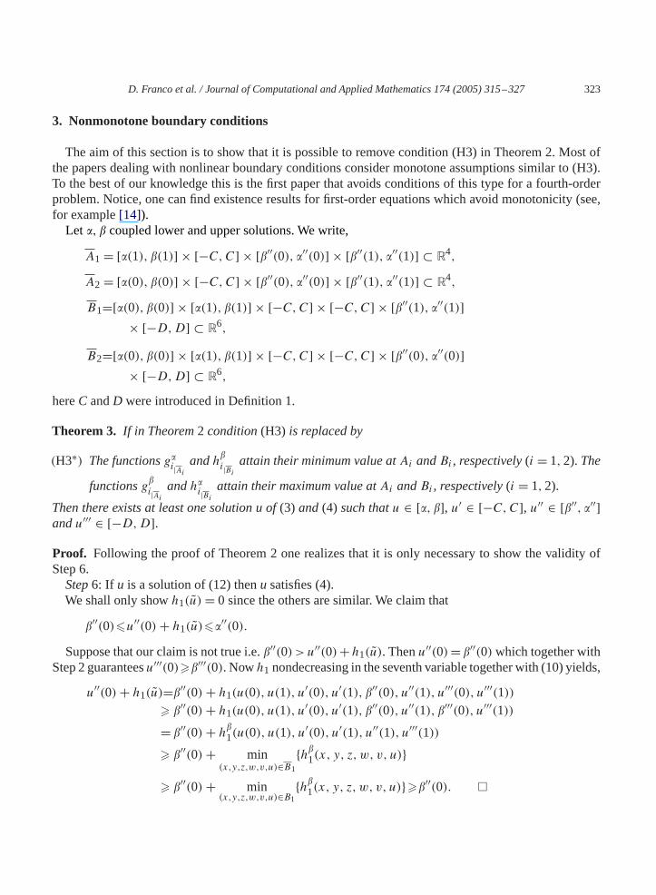
3. Nonmonotone boundary conditions

The aim of this section is to show that it is possible to remove condition (H3) in Theorem 2. Most ofthe papers dealing with nonlinear boundary conditions consider monotone assumptions similar to (H3).To the best of our knowledge this is the first paper that avoids conditions of this type for a fourth-orderproblem. Notice, one can find existence results for first-order equations which avoid monotonicity (see,for example[14]).

Let �, � coupled lower and upper solutions. We write,

A1 = [�(1), �(1)] × [−C,C] × [�′′(0), �′′(0)] × [�′′(1), �′′(1)] ⊂ R4,

A2 = [�(0), �(0)] × [−C,C] × [�′′(0), �′′(0)] × [�′′(1), �′′(1)] ⊂ R4,

B1=[�(0), �(0)] × [�(1), �(1)] × [−C,C] × [−C,C] × [�′′(1), �′′(1)]× [−D,D] ⊂ R6,

B2=[�(0), �(0)] × [�(1), �(1)] × [−C,C] × [−C,C] × [�′′(0), �′′(0)]× [−D,D] ⊂ R6,

hereC andD were introduced in Definition 1.

Theorem 3. If in Theorem2 condition(H3) is replaced by

(H3∗) The functionsg�i|Ai

andh�i|Bi

attain their minimum value atAi andBi , respectively(i = 1,2).The

functionsg�i|Ai

andh�i|Bi

attain their maximum value atAi andBi , respectively(i = 1,2).

Then there exists at least one solution u of(3) and(4) such thatu ∈ [�, �], u′ ∈ [−C,C], u′′ ∈ [�′′, �′′]andu′′′ ∈ [−D,D].Proof. Following the proof of Theorem 2 one realizes that it is only necessary to show the validity ofStep 6.Step6: If u is a solution of (12) thenu satisfies (4).We shall only showh1(u)= 0 since the others are similar. We claim that

�′′(0)�u′′(0)+ h1(u)��′′(0).

Suppose that our claim is not true i.e.�′′(0)>u′′(0)+ h1(u). Thenu′′(0)= �′′(0) which together withStep 2 guaranteesu′′′(0)��′′′(0). Nowh1 nondecreasing in the seventh variable together with (10) yields,

u′′(0)+ h1(u)=�′′(0)+ h1(u(0), u(1), u′(0), u′(1), �′′(0), u′′(1), u′′′(0), u′′′(1))

� �′′(0)+ h1(u(0), u(1), u′(0), u′(1), �′′(0), u′′(1), �′′′(0), u′′′(1))

= �′′(0)+ h�1(u(0), u(1), u

′(0), u′(1), u′′(1), u′′′(1))� �′′(0)+ min

(x,y,z,w,v,u)∈B1

{h�1(x, y, z, w, v, u)}

� �′′(0)+ min(x,y,z,w,v,u)∈B1

{h�1(x, y, z, w, v, u)}��′′(0). �

324 D. Franco et al. / Journal of Computational and Applied Mathematics 174 (2005) 315–327

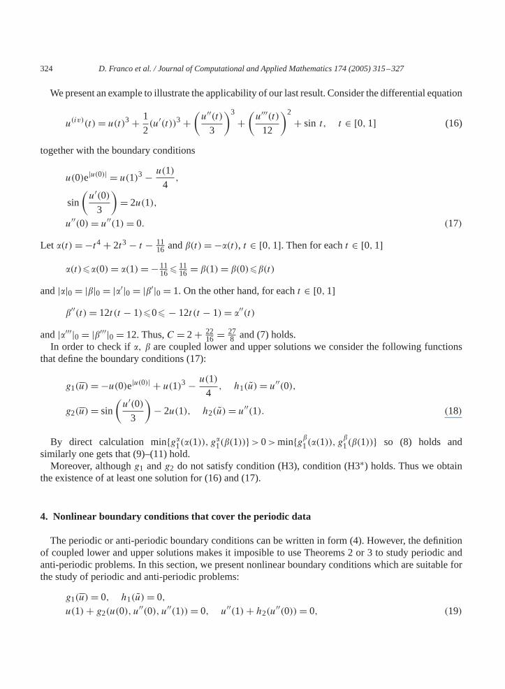
We present an example to illustrate the applicability of our last result. Consider the differential equation

u(iv)(t)= u(t)3 + 1

2(u′(t))3 +

(u′′(t)

3

)3

+(u′′′(t)

12

)2

+ sin t, t ∈ [0,1] (16)

together with the boundary conditions

u(0)e|u(0)| = u(1)3 − u(1)

4,

sin

(u′(0)

3

)= 2u(1),

u′′(0)= u′′(1)= 0. (17)

Let �(t)= −t4 + 2t3 − t − 1116 and�(t)= −�(t), t ∈ [0,1]. Then for eacht ∈ [0,1]

�(t)��(0)= �(1)= −1116� 11

16 = �(1)= �(0)��(t)

and|�|0 = |�|0 = |�′|0 = |�′|0 = 1. On the other hand, for eacht ∈ [0,1]�′′(t)= 12t (t − 1)�0� − 12t (t − 1)= �′′(t)

and|�′′′|0 = |�′′′|0 = 12. Thus,C = 2 + 2216 = 27

8 and (7) holds.In order to check if�, � are coupled lower and upper solutions we consider the following functions

that define the boundary conditions (17):

g1(u)= −u(0)e|u(0)| + u(1)3 − u(1)

4, h1(u)= u′′(0),

g2(u)= sin

(u′(0)

3

)− 2u(1), h2(u)= u′′(1). (18)

By direct calculation min{g�1(�(1)), g

�1(�(1))}>0>min{g�

1(�(1)), g�1(�(1))} so (8) holds and

similarly one gets that (9)–(11) hold.Moreover, althoughg1 andg2 do not satisfy condition (H3), condition (H3∗) holds. Thus we obtain

the existence of at least one solution for (16) and (17).

4. Nonlinear boundary conditions that cover the periodic data

The periodic or anti-periodic boundary conditions can be written in form (4). However, the definitionof coupled lower and upper solutions makes it imposible to use Theorems 2 or 3 to study periodic andanti-periodic problems. In this section, we present nonlinear boundary conditions which are suitable forthe study of periodic and anti-periodic problems:

g1(u)= 0, h1(u)= 0,u(1)+ g2(u(0), u

′′(0), u′′(1))= 0, u′′(1)+ h2(u′′(0))= 0, (19)

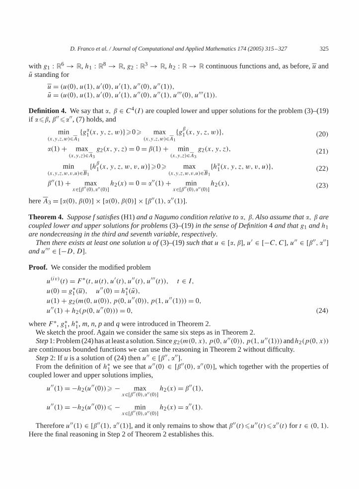
D. Franco et al. / Journal of Computational and Applied Mathematics 174 (2005) 315–327 325

with g1 : R6 → R, h1 : R8 → R, g2 : R3 → R, h2 : R → R continuous functions and, as before,u andu standing for

u= (u(0), u(1), u′(0), u′(1), u′′(0), u′′(1)),u= (u(0), u(1), u′(0), u′(1), u′′(0), u′′(1), u′′′(0), u′′′(1)).

Definition 4. We say that�, � ∈ C4(I ) are coupled lower and upper solutions for the problem (3)–(19)if ���, �′′��′′, (7) holds, and

min(x,y,z,w)∈A1

{g�1(x, y, z, w)}�0� max

(x,y,z,w)∈A1

{g�1(x, y, z, w)}, (20)

�(1)+ max(x,y,z)∈A3

g2(x, y, z)= 0 = �(1)+ min(x,y,z)∈A3

g2(x, y, z), (21)

min(x,y,z,w,v,u)∈B1

{h�1(x, y, z, w, v, u)}�0� max

(x,y,z,w,v,u)∈B1

{h�1(x, y, z, w, v, u)}, (22)

�′′(1)+ maxx∈[�′′(0),�′′(0)]

h2(x)= 0 = �′′(1)+ minx∈[�′′(0),�′′(0)]

h2(x), (23)

hereA3 = [�(0), �(0)] × [�(0), �(0)] × [�′′(1), �′′(1)].Theorem 4. Suppose f satisfies(H1) and a Nagumo condition relative to�, �.Also assume that�, � arecoupled lower and upper solutions for problems(3)–(19)in the sense of Definition4 and thatg1 andh1are nondecreasing in the third and seventh variable, respectively.Then there exists at least one solution u of(3)–(19)such thatu ∈ [�, �], u′ ∈ [−C,C], u′′ ∈ [�′′, �′′]

andu′′′ ∈ [−D,D].Proof. We consider the modified problem

u(iv)(t)= F ∗(t, u(t), u′(t), u′′(t), u′′′(t)), t ∈ I,u(0)= g∗

1(u), u′′(0)= h∗1(u),

u(1)+ g2(m(0, u(0)), p(0, u′′(0)), p(1, u′′(1)))= 0,

u′′(1)+ h2(p(0, u′′(0)))= 0, (24)

whereF ∗, g∗1, h∗

1, m, n, p andqwere introduced in Theorem 2.We sketch the proof. Again we consider the same six steps as in Theorem 2.Step1: Problem (24) has at least a solution. Sinceg2(m(0, x), p(0, u′′(0)), p(1, u′′(1)))andh2(p(0, x))

are continuous bounded functions we can use the reasoning in Theorem 2 without difficulty.Step2: If u is a solution of (24) thenu′′ ∈ [�′′, �′′].From the definition ofh∗

1 we see thatu′′(0) ∈ [�′′(0), �′′(0)], which together with the properties ofcoupled lower and upper solutions implies,

u′′(1)= −h2(u′′(0))� − max

x∈[�′′(0),�′′(0)]h2(x)= �′′(1),

u′′(1)= −h2(u′′(0))� − min

x∈[�′′(0),�′′(0)]h2(x)= �′′(1).

Thereforeu′′(1) ∈ [�′′(1), �′′(1)], and it only remains to show that�′′(t)�u′′(t)��′′(t) for t ∈ (0,1).Here the final reasoning in Step 2 of Theorem 2 establishes this.

326 D. Franco et al. / Journal of Computational and Applied Mathematics 174 (2005) 315–327

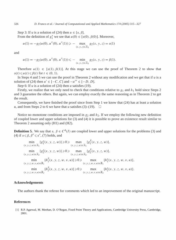
Step3: If u is a solution of (24) thenu ∈ [�, �].From the definition ofg∗

1 we see thatu(0) ∈ [�(0), �(0)]. Moreover,

u(1)= −g2(u(0), u′′(0), u′′(1))� − max

(x,y,z)∈A3

g2(x, y, z)= �(1)

and

u(1)= −g2(u(0), u′′(0), u′′(1))� − min

(x,y,z)∈A3

g2(x, y, z)= �(1).

Thereforeu(1) ∈ [�(1), �(1)]. At this stage we can use the proof of Theorem 2 to show that�(t)�u(t)��(t) for t ∈ (0,1).

In Steps 4 and 5 we can use the proof in Theorem 2 without any modification and we get that ifu is asolution of (24) thenu′ ∈ [−C,C] and−u′′′ ∈ [−D,D].Step6: If u is a solution of (24) thenu satisfies (19).Firstly, we realize that we only need to check that conditions relative tog1 andh1 hold since Steps 2

and 3 guarantee the others. But again, we can employ exactly the same reasoning as in Theorem 2 to getthe result.

Consequently, we have finished the proof since from Step 1 we know that (24) has at least a solutionu, and from Steps 2 to 6 we have thatu satisfies (3)–(19). �

Notice no monotone conditions are imposed ing2 andh2. If we employ the following new definitionof coupled lower and upper solutions for (3) and (4) it is possible to prove an existence result similar toTheorem 2 assuming only (H1) and (H2).

Definition 5. We say that�, � ∈ C4(I ) are coupled lower and upper solutions for the problems (3) and(4) if ���, �′′��′′, (7) holds, and

min(x,y,z,w)∈A1

{g�1(x, y, z, w)}�0� max

(x,y,z,w)∈A1

{g�1(x, y, z, w)},

min(x,y,z,w)∈A2

{g�2(x, y, z, w)}�0� max

(x,y,z,w)∈A2

{g�2(x, y, z, w)},

min(x,y,z,w,v,u)∈B1

{h�1(x, y, z, w, v, u)}�0� max

(x,y,z,w,v,u)∈B1

{h�1(x, y, z, w, v, u)},

min(x,y,z,w,v,u)∈B2

{h�2(x, y, z, w, v, u)}�0� max

(x,y,z,w,v,u)∈B2

{h�2(x, y, z, w, v, u)}.

Acknowledgements

The authors thank the referee for comments which led to an improvement of the original manuscript.

References

[1] R.P. Agarwal, M. Meehan, D. O’Regan, Fixed Point Theory and Applications, Cambridge University Press, Cambridge,2001.

D. Franco et al. / Journal of Computational and Applied Mathematics 174 (2005) 315–327 327

[2] Z. Bai, The method of lower and upper solutions for a bending of an elastic beam equation, J. Math. Anal. Appl. 248 (2000)195–202.

[3] A. Cabada, The method of lower and upper solutions for second, third, fourth and higher order boundary value problems,J. Math. Anal. Appl. 185 (1994) 302–320.

[4] A. Cabada, R.L. Pouso, Existence results for the problem(�(u′))′ = f (t, u, u′) with nonlinear boundary conditions,Nonlinear Anal. 35 (1999) 221–231.

[5] P. Drávek, G. Holubová, A. Matas, P. Ne˘cesal, Nonlinear models of suspension bridges: discussion of the results, Appl.Math. 6 (2003) 497–514.

[6] J. Ehme, P.W. Eloe, J. Henderson, Existence of solutions 2nd order fully nonlinear generalized Sturm–Liouville boundaryvalue problems, Math. Inequal. Appl. 4 (2001) 247–255.

[7] J. Ehme, P.W. Eloe, J. Henderson, Upper and lower solution methods for fully nonlinear boundary value problems,J. Differential Equations 180 (2002) 51–64.

[8] L.H. Erbe, Nonlinear boundary value problems for second order differential equations, J. Differential Equations 7 (1970)459–472.

[9] Ch. Fabry, P. Habets, Upper and lower solutions for second-order boundary value problems with nonlinear boundaryconditions, Nonlinear Anal. 10 (1986) 985–1007.

[10] D. Franco, J.J. Nieto, D. O’Regan, Anti-periodic boundary value problem for nonlinear first order ordinary differentialequations, Math. Inequal. Appl. 6 (2003) 477–485.

[11] D. Franco, D. O’Regan, A new upper and lower solutions approach for second order problems with nonlinear boundaryconditions, Arch. Inequal. Appl. 1 (2003) 413–420.

[12] P. Hartman, Ordinary Differential Equations, Wiley, New York, 1964.[13] G. Infante, Positive solutions of differential equations with nonlinear boundary conditions, Discrete Contin. Dynamic

Systems (special volume) (2003) 432–438.[14] I.T. Kiguradze, B. Pu˘za, Some boundary-value problems for a system of ordinary differential equations, Differential

Equations 12 (1977) 1493–1500.[15] R.Y. Ma, J.H. Zhang, S.M. Fu, The method of lower and upper solutions for fourth-order two-point boundary value

problems, J. Math. Anal. Appl. 215 (1997) 415–422.[16] J. Mawhin, K. Schmitt, Upper and lower solutions and semilinear second order elliptic equations with nonlinear boundary

conditions, Proc. Roy. Soc. Edinburgh Sect. A 97 (1984) 199–207.[17] M.A. Peletier, Generalized monotonicity from global minimization in fourth-order ordinary differential equations,

Nonlinearity 14 (2001) 1221–1238.[18] I. Rachunková, J. Tomeˇcek, On nonlinear boundary value problem for systems of differential equations with impulses,

Acta Univ. Palack. Olomuc. Fac. Rerum Natur. Math. 41 (2002) 119–129.[19] P.J.Y. Wong, R.P. Agarwal, Eigenvalues of Lidstone boundary value problems, Appl. Math. Comput. 104 (1999) 15–31.