On the Boundary Ergodic Problem for Fully Nonlinear ...barles/ergodicbounded.pdf · with General Nonlinear Neumann Boundary Conditions ... This was the motivation of Lions, Papanicolaou

On the Boundary Ergodic Problem for FullyNonlinear Equations in Bounded Domains

with General Nonlinear Neumann BoundaryConditions

Guy Barles(1) & Francesca Da Lio(2)

31st August 2004

Abstract

We study nonlinear Neumann type boundary value problems related to ergodicphenomenas. The particularity of these problems is that the ergodic constant ap-pears in the (possibly nonlinear) Neumann boundary conditions. We provide, forbounded domains, several results on the existence, uniqueness and properties of thisergodic constant.

1 Introduction

In this article, we are interested in what can be called “boundary ergodic control problems”which lead us to solve the following type of fully nonlinear elliptic equations associatedwith nonlinear Neumann boundary conditions

F (x,Du,D2u) = λ in O, (1)

L(x,Du) = µ on ∂O, (2)

where, say, O ⊂ Rn is a smooth domain, F and L are, at least, continuous functionsdefined respectively on O×Rn ×Sn and O×Rn with values in R, where Sn denotes thespace of real, n×n, symmetric matrices. More precise assumptions on F and L are givenlater on.

(1)Laboratoire de Mathematiques et Physique Theorique. Universite de Tours. Faculte des Sciences etTechniques, Parc de Grandmont, 37200 Tours, France.

(2)Dipartimento di Matematica. Universita di Torino. Via Carlo Alberto 10, 10123 Torino, Italy.

1

The solution u of this nonlinear problem is scalar and Du, D2u denote respectivelygradient and Hessian matrix of u. Finally, λ, µ are constants : µ, which is called belowthe “boundary ergodic cost”, is part of the unknowns while λ is mainly here consideredas a given constant for reasons explained below.

In order to justify the study of such problems, we first concentrate only on the equation(1), without boundary condition, i.e. on the case when O = Rn. In this framework, undersuitable assumptions on F , the typical result that one expects is the following : there existsa unique constant λ such that (1) has a bounded solution. Such results were first provedfor first-order equations by Lions, Papanicolaou & Varadhan [37] (see also Concordel [22])in the case of periodic equations and solutions. Recently, Ishii [31] generalizes these resultsin the almost periodic case. General results for second-order equations in the periodicsetting are proved by Evans [25, 26]. Results in the evolution case, when the equation isperiodic both in space and time, were also obtained recently by Souganidis and the firstauthor [16] : the methods of [16], translated properly to the stationary case, are the onewho would lead to the most general results in the case of second-order equations. All theseresults which hold for general equations without taking advantage of their particularities,are complemented by more particular results in the applications we describe now.

The first application concerns the so-called ergodic control problems (either in thedeterministic or stochastic case). We refer to Bensoussan [17] for an introduction to suchproblems and to Bensoussan & Frehse [18], Bagagiolo, Bardi & Capuzzo Dolcetta [7],Arisawa [3, 4], Arisawa & Lions [6] for further developments in the Rn case and withdifferent types of pde approaches. In this framework, (1) is the Bellman Equation of theergodic control problem, λ is the ergodic cost and the solution u is the value function ofthe control problem. In this case, both the uniqueness of λ and of u – which can holdonly up to an additive constant – is interesting for the applications. But it is rather easyto obtain the uniqueness of λ in general, while the uniqueness of u can be proved only inthe uniformly elliptic case and is generally false.

A second motivation to look at such problems is the asymptotic behavior as t → ∞of solutions of the evolution equation

ut + F (x,Du,D2u) = 0 in Rn × (0,+∞) . (3)

A typical result here is the following : if there exists a unique λ such that (1) has asolution (typically in the bounded solutions framework), then one should have

u(x, t)

t→ λ locally uniformly as t→∞ .

Therefore the ergodic constant governs the asymptotic behavior of the associated evolutionequation and in good cases, one can even show that

u(x, t)− λt→ u∞(x) as t→∞ ,

where u∞ solves (1).

2

Such results were obtained recently, for first-order equations, by Fathi [28, 29, 30]and Namah & Roquejoffre [39] in the case when F is convex in Du ; these results weregeneralized and extended to a non-convex framework in Barles & Souganidis [15]. To thebest of our knowledge, there is not a lot of general results in the case of second-orderequations : the uniformly elliptic case seems the only one which is duable through the useof the Strong Maximum Principle and the methods of [16] which are used in the paperto prove the convergence to space-time periodic solutions but which can be used to showthe convergence to solutions of the stationary equations.

The third and last application (and maybe the most interesting one) concerns homog-enization of elliptic and parabolic pdes. This was the motivation of Lions, Papanicolaou& Varadhan [37] to study these types of ergodic problems as it was also the one of Evans[25, 26]. The ergodic problem is nothing but the so-called “cell problem” in homogeniza-tion theory, λ being connected to the “effective equation”. We also refer the reader toConcordel [23], Evans & Gomes [27], Ishii [31] for results in this direction. The connec-tions between ergodic problems and homogenization are studied in a systematic way inAlvarez & Bardi [1, 2] and completely clarified.

Of course, the same questions have been studied in bounded (or unbounded) domainswith suitable boundary conditions. For first-order equations, Lions [36] studies the er-godic problem in the case of homogeneous Neumann boundary conditions, while CapuzzoDolcetta & Lions [21] study it in the case of state-constraints boundary conditions. Forsecond-order equations, we refer the reader to Bensoussan & Frehse [19] in the case of ho-mogeneous Neumann boundary conditions and to Lasry & Lions [35] for state-constraintsboundary conditions. It is worth pointing out that in all these works, the constant µ doesnot appear and the authors are interested in the constant λ instead.

The first and, to the best of our knowledge, only work where the problem of the con-stant µ appears, is the one of Arisawa [5]. In this work, she studies two different cases :the case of bounded domains which we consider here and the case of half-space type do-mains which contains different difficulties; we address this problem in a forthcoming workin collaboration with P.L. Lions and P.E. Souganidis. In the case of bounded domains,we improve her results in several directions : generality and regularity of the equationand boundary condition, possibility of obtaining results in degenerate cases, uniquenessin more general frameworks, interpretation in terms of stochastic control problems andconnections of these types of ergodic problems with large time behavior of solutions ofinitial value problem with Neumann boundary conditions. We are able to do so since weuse softer viscosity solutions’ methods.

It is worth pointing out that the role of the two constants are different : our mainresults say that, for any λ, there exists a unique constant µ := µ(λ) for which (1)-(2)has a bounded solution. Therefore the role played previously by λ is now played by µ.To prove such a result, we have to require some uniform ellipticity assumption on F , notonly in order to obtain the key estimates which are needed to prove the existence of thesolution u but also because µ can play its role only if the boundary condition is “seen in

3

a right way by the equation”. Indeed, the counter-example of Arisawa [5], p. 312, showsthat otherwise µ cannot be unique. This vague statement is partly justified in Section 6.

The proof of the existence of the solution relies on the C0,α estimates proved in [12];in order to have an as self-contained paper as possible, we describe these results in theAppendix. Here also the uniform ellipticity of F plays a role, at least in the case whenthe Neumann boundary condition is indeed nonlinear. But if the boundary condition islinear, some less restrictive ellipticity assumptions on F can be made : this is the reasonwhy we distinguish the two cases below.

An other question we address in this paper, are the connections with the large timebehavior of the solutions of the two different type of evolution problems

vt + F (x,Dv,D2v) = λ in O × (0,+∞), (4)

L(x,Dv) = µ on ∂O × (0,+∞). (5)

and

wt + F (x,Dw,D2w) = 0 in O × (0,+∞), (6)

wt + L(x,Dw) = 0 on ∂O × (0,+∞). (7)

In the case of (4)-(5), we show that the ergodic constant µ(λ) is characterized as theonly constant µ for which the solution v remains bounded. In the case of (6)-(7), theexpected behavior is to have t−1w(x, t) converging to a constant λ which has to be suchthat (1)-(2) has a solution for λ = λ = µ(λ). We prove that, under suitable conditions,such a constant λ, i.e. a fixed point of the map λ 7→ µ(λ), does exist and that we havethe expected behavior at infinity for w.

Finally we consider the case when the equation is the Hamilton-Jacobi-Bellman Equa-tion of a stochastic control problem with reflection : this gives us the opportunity torevisit the results on the uniqueness of µ in a degenerate context and to provide a formulaof representation for µ.

The paper is organized as follows. In Section 2, we prove the existence of u and µ inthe case of nonlinear boundary conditions while in Section 3 we treat the linear case. InSection 4, we examine the uniqueness properties for µ together with its dependence in λ,F and L; among the results of this part, there is the existence of λ. Section 5 is devotedto present the results connecting the ergodic problem with the asymptotic behavior ofsolution of some nonlinear problem. Finally we study the connections with stochasticcontrol problem with reflection in Section 6.

2 The case of nonlinear boundary conditions

To state our result, we use the following assumptions

(O1) O is a bounded domain with a W 3,∞ boundary.

4

We point out that such assumption on the regularity of the boundary is needed bothin order to use the comparison results of [11] (here the W 3,∞ regularity is needed) andthe local C0,α-estimates of [12] (here a C2 regularity would be enough).

We denote by d the sign-distance function to ∂O which is positive in O and negative inRn \O. If x ∈ ∂O, we recall that Dd(x) = −n(x) where n(x) is the outward unit normalvector to ∂O at x. The main consequence of (O1) is that d is W 3,∞ in a neighborhoodof ∂O.

Next we present the assumptions on F and L.

(F1) (Regularity) The function F is locally Lipschitz continuous on O × Rn × Sn andthere exists a constant K > 0 such that, for any x, y ∈ O, p, q ∈ Rn, M,N ∈ Sn

|F (x, p,M)−F (y, q,N)| ≤ K |x− y|(1 + |p|+ |q|+ ||M ||+ ||N ||) + |p− q|+ ||M −N || .

(F2) (Uniform ellipticity) There exists κ > 0 such that, for any x ∈ O, p ∈ Rn,M,N ∈ Sn with N ≥ 0

F (x, p,M +N)− F (x, p,M) ≤ −κTr(N) .

(F3) There exists a continuous function F∞ such that

t−1F (x, tp, tM) → F∞(x, p,M) locally uniformly, as t→ +∞ .

For the boundary condition L, we use the following assumptions.

(L1) There exists ν > 0 such that, for all (x, p) ∈ ∂O × Rn and t > 0, we have

L(x, p+ tn(x))− L(x, p) ≥ νt . (8)

(L2) There is a constant K > 0 such that, for all x, y ∈ ∂O, p, q ∈ Rn, we have

|L(x, p)− L(y, q)| ≤ K [(1 + |p|+ |q|)|x− y|+ |p− q|] . (9)

(L3) There exists a continuous function L∞ such that

t−1L(x, tp) → L∞(x, p) locally uniformly, as t→ +∞ .

Before stating and proving the main result of this section, we want to emphasizethe fact that the above assumptions are very well adapted for applications to stochasticcontrol and differential games: indeed (F1)-(L1) are clearly satisfied as soon as thedynamic has bounded and Lipschitz continuous drift, diffusion matrix and direction ofreflection and when the running and boundary cost satifies analogous properties (maybethese assumptions are not optimal but they are rather natural) while (F3)-(L3) arealmost obviously satisfied because of the structure of the Bellman or Isaac Equations(“sup” or “inf sup” of affine functions in p and M).

Our result is the

5

Theorem 2.1 Assume (O1), (F1)-(F3) and (L1)-(L3) then, for any λ ∈ R, thereexists µ ∈ R such that (1)-(2) has a continuous viscosity solution.

Proof. The proof follows the strategy of Arisawa [5]. For 0 < ε α 1, we introducethe approximate problem

F (x,Du,D2u) + εu = λ in O, (10)

L(x,Du) + αu = 0 on ∂O. (11)

1. It is more or less standard to prove that this problem has a unique continuous viscositysolution using the Perron’s method of Ishii [32] and the comparison arguments of Barles[11]; the only slight difficulty comes from the x-dependence of F which is a priori notsufficient to obtain a suitable comparison. In the Appendix, we explain why the usualapproach does not work and we show how to overcome this difficulty by borrowing ideasof Barles & Ramaswamy [14].2. The next step consists in obtaining basic estimates on u. We drop the dependence ofu in ε and α for the sake of simplicity of notations. To do so, we use the fact that O isbounded and therefore we can assume without loss of generality that O ⊂ x1 > 0.

We introduce the smooth functions

u(x) = C(2− exp(−γx1)) , u(x) = −C(2− exp(−γx1)) .

Notice that u < 0 < u on O.By using (F1) and (F2), one sees that, for γ and C large enough, one has

F (x,Du,D2u) ≥ F (x, 0, 0)

− KCγ exp(−γx1) + kCγ2 exp(−γx1) > 0 ,

and

F (x,Du,D2u) ≤ F (x, 0, 0)

+ KCγ exp(−γx1)− kCγ2 exp(−γx1) < 0 .

Next we consider maxO(u − u) and minO(u − u) which are achieved respectively atx1, x2 ∈ O. Because of the above properties and since u is a viscosity solution of (10)-(11),these max and min cannot be achieved in O and, in any case, the “F” inequalities cannothold. The “L” inequalities lead to the estimates

αu(x) ≤ α(u(x)− u(x1)) + supO|L(x,Du(x))| ,

andαu(x) ≥ α(u(x)− u(x2))− sup

O|L(x,Du(x))|

6

for every x ∈ O. Thus for some positive constant C(F,L) (depending on F and L) wehave

||αu||∞ ≤ C(F,L) . (12)

3. Let x0 be any point of O and set v(x) = u(x) − u(x0) for x ∈ O. We claim that vremains uniformly bounded as α tends to 0 if ε α.

To prove the claim, we argue by contradiction assuming that M := ||v||∞ → ∞ asα→ 0 and we set w(x) := M−1v(x). The function w solves

M−1F (x,MDw,MD2w) + εw = M−1λ−M−1εu(x0) in O, (13)

M−1L(x,Dw) + αw = −M−1αu(x0) on ∂O. (14)

Moreover ||w||∞ = 1 and w(x0) = 0.Since w is uniformly bounded, the C0,β regularity results and estimates of Barles &

Da Lio [12] apply and therefore w is uniformly bounded in C0,β, for any 0 < β < 1 (seealso the Appendix, for a description of these results) .

Using Ascoli’s Theorem, one may assume without loss of generality that w convergesuniformly to some C0,β-function w and taking (F3)-(L3) in account, the stability resultsfor viscosity solutions implies that w solves

F∞(x,Dw,D2w) = 0 in O, (15)

L∞(x,Dw) = 0 on ∂O. (16)

Moreover ||w||∞ = 1 and w(x0) = 0.We are going to show now that all these properties lead to a contradiction by Strong

Maximum Principle type arguments. Since w is continuous there exists x ∈ O such that|w(x)| = 1.

We first remark that F∞ satisfies (F1)-(F2) as well and is homogeneous of degree 1;therefore the Strong Maximum Principle of Bardi & Da Lio [8] implies that necessarilyx ∈ ∂O. In fact −1 < w < 1 in O.

We assume for example that w(x) = 1, the other case being treated similarly. Toconclude, we are going to use the following lemma.

Lemma 2.1 There exists r > 0 and a smooth function ϕ on B(x, r) such that ϕ(x) = 0,ϕ(y) > 0 on ∂O ∩B(x, r) \ x

F∞(y,Dϕ(y), D2ϕ(y)) > 0 on B(x, r) , (17)

andDϕ(x) = kn(x) ,

with k > 0.

7

The proof of this lemma is given in the Appendix; we show how to use it in order toconclude.

Since Dϕ(x) = kn(x), we have L∞(x,Dϕ(x)) > 0. But ϕ is smooth and therefore, bychoosing θ < r small enough, we have also

L∞(y,Dϕ(y)) > 0 on B(x, θ) ∩ ∂O . (18)

On an other hand, by choosing τ > 0 small enough, we can have w(y) − τϕ(y) < 1 =w(x) − τϕ(x) for y ∈ ∂B(x, θ) ∩ O. Indeed, for y close to ∂O, ϕ(y) > 0 while in O wehave w(y) < 1.

We deduce from this property that, if we consider maxB(x,θ)∩O(w−τϕ), this maximum

is necessarely achieved in B(x, θ)∩O and therefore it is a local maximum point of w− τϕbut, taking in account the fact that F∞ and L∞ are homogeneous of degree 1, this is acontradiction with the inequalities (17)-(18).4. From step 3, the functions v are uniformly bounded and solve

F (x,Dv,D2v) + εv = λ− εu(x0) in O, (19)

L(x,Dv) + αv = −αu(x0) on ∂O. (20)

Using again the regularity results of Barles & Da Lio [12] (see also the Appendix), wededuce that the functions v are also uniformly bounded in C0,β for any 0 < β < 1 andby Ascoli’s Theorem, extracting if necessary a subsequence, we may assume that theyconverge uniformly to a function u ∈ C0,β(O). Moreover, since αu is also uniformlybounded, we can also extract a subsequence such that −αu(x0) converges to some µ ∈ R.

In order to conclude, we just pass to the limit in (19)-(20) with a choice of ε such thatεα−1 → 0.

3 The case of linear boundary conditions

We consider in this section the case when L is given by

〈Du, γ(x)〉+ g(x) = µ on ∂O, (21)

where the functions γ and g satisfies

(L1’) g ∈ C0,β(∂O) for some 0 < β ≤ 1 and γ is a Lipschitz continuous function, takingvalues in Rn and such that 〈γ(x), n(x)〉 ≥ ν > 0 for any x ∈ ∂O, where we recall thatn(x) denotes the unit exterior normal vector to ∂O at x.

In this linear case, we are able to weaken the ellipticity assumption on F . In the

following, for q ∈ Rn, the notation q stands forq

|q|.

8

(F2’) (partial uniform ellipticity) There exists a Lipschitz continuous function x 7→A(x), defined on O and taking value in the space of symmetric, definite positive matrixand κ > 0 such that

(i) for any x ∈ ∂O, A(x)γ(x) = n(x),(ii) for any x ∈ O, p ∈ Rn \ 0, M,N ∈ Sn with N ≥ 0

F (x, p,M +N)− F (x, p,M) ≤ −κ〈Nq, q〉+ o(1)||N || ,

with q = A−1(x)p and where o(1) denotes a function of |p| which converges to 0 as |p|tends to +∞.

If γ ≡ n, this assumption is satisfied in particular if (formally)

FM(x, p,M) ≤ −κp⊗ p+ o(1) a.e. in O × Rn × Sn ,

where, as above, o(1) denotes a function of |p| which converges to 0 as |p| tends to +∞;this means a non-degeneracy property in the gradient direction, at least for large |p|. Thiscorresponds to the choice A(x) ≡ Id. We recall that for all p ∈ Rn, p ⊗ p denotes thesymmetric matrix defined by (p⊗ p)ij = pipj.

In this case, unlike the uniform elliptic case, (F2’) is not enough to ensure a compar-ison property for F , thus we add

(F4’) For any K > 0, there exists a function mK : R+ → Rn such that mK(t) → 0 whent→ 0 and such that, for all η > 0

F (y, q, Y )− F (x, p,X) ≤ mK

(η + |x− y|(1 + |p| ∨ |q|) +

|x− y|2

ε2

)for all x, y ∈ O, p, q ∈ Rn and for all matrices X, Y ∈ Sn satisfying the following

properties

−Kε2Id ≤

(X 00 −Y

)≤ K

ε2

(Id −Id−Id Id

)+ KηId , (22)

|p− q| ≤ Kηε(1 + |p| ∧ |q|) , (23)

|x− y| ≤ Kηε. (24)

Our result is the

Theorem 3.1 Assume (F1)-(F2’)-(F3)-(F4’) and (L1’) then, for any λ ∈ R, thereexists µ ∈ R such that (1)-(2) has a continuous viscosity solution.

We skip the proof since it follows readily the one of Theorem 2.1; we just point outthat the key C0,β-estimates follow from the linear case in [12] (see also the Appendix)while the Strong Maximum Principle still holds under (F2’) as we pointed it out in theAppendix.

9

4 Uniqueness results for the boundary ergodic cost

In standard problems, the uniqueness of the ergodic cost is rather easy to obtain, whilethe uniqueness of the solution u is a more difficult question. Here, even the uniquenessof µ is a non obvious fact because µ appears only in the boundary condition and clearlythis boundary condition has to be sufficiently “seen” in order to have such a uniquenessproperty. The counter-example of Arisawa [5] for first-order equations shows that, in thecases where losses of boundary conditions can occur, µ is not unique in general.

To state the uniqueness result, we introduce the following abstract assumption

(U1) If w is an upper semicontinuous viscosity subsolution of (1)-(2), there exists asequence (wε)ε of upper semicontinuous functions such that lim sup∗wε = w on O, (1)

satisfying in the viscosity sense

F (x,Dwε, D2wε) ≤ λε < λ in O, (25)

L(x,Dwε) ≤ µ+ oε(1) on ∂O. (26)

Our result is the

Theorem 4.1 Under the assumptions of either Theorem 2.1 or 3.1 and if (U1) holds,if u1 is a subsolution of (1)-(2) associated to λ1, µ1 and if u2 is a supersolution of (1)-(2)associated to λ2, µ2 with λ1 ≤ λ2 then necessarily µ1 ≥ µ2. In particular, for any λ, theboundary ergodic cost µ is unique.

Proof. We argue by contradiction assuming that µ1 < µ2.Let uε

1 be a continuous function associated to u1 through assumption (U1) with εchoosen in such a way that

L(x,Duε1) ≤ µ on ∂O,

where µ :=1

2(µ1 + µ2).

We consider maxO×O (uε1(x) − u2(y) − ψα(x, y)) where for all α > 0 ψα is the test-

function built in [11] for the boundary condition L− µ (we recall that this test-functiondepends only on the boundary condition).

Following readily the arguments of [11], one is led to the inequalities

F (x, p,X) ≤ λ1,ε < λ1 , (27)

F (y, q, Y ) ≥ λ2 , (28)

(1)We recall that the half-relaxed limit lim sup∗wε is defined by : lim sup∗wε(x) = lim supy→xε→0

wε(y) for any

x ∈ O.

10

where (p,X) ∈ D2,+uε1(x) and (q, Y ) ∈ D2,−u2(y). Then either the standard comparison

arguments or the arguments of [14] shows that

F (x, p,X)− F (y, q, Y ) ≥ oα(1) ,

and hence, by subtracting the inequalities (27) and (28), we have oα(1) ≤ λ1,ε − λ2 < 0.We get the contradiction by letting α tends to 0. And the proof of the first part iscomplete.

Of course, the uniqueness of the boundary ergodic cost follows since, if u and v aretwo solutions of (1)-(2) with the same λ and roles with µ, µ respectively, we can applythe above result with u1 = u, µ1 = µ, λ1 = λ and u2 = v, µ2 = µ, λ2 = λ : this yieldsµ1 ≥ µ2. But using that the two solutions play symmetric roles, we deduce immediatelyµ = µ, i.e. the uniqueness of the ergodic cost.

Remark 4.1 As the proof shows it, the result “µ1 ≤ µ2 ⇒ λ1 ≥ λ2” is easy to obtainwithout assuming (U1), just as a straightforward consequence of the comparison argu-ments. It is therefore true as soon as F and L satisfy the conditions of the comparisonresult, i.e. under far weaker assumptions than the result of Theorem 4.1. The key pointin Theorem 4.1 is really the result “µ1 < µ2 ⇒ λ1 > λ2” .

Now we turn to the checking of (U1) which can be formulated in the following way.

Theorem 4.2 The boundary ergodic cost µ is unique in the two following cases

(i) under the assumption of Theorem 2.1,

(ii) under the assumption of Theorem 3.1 on F and of Theorem 2.1 on L, if F (x, p,M)is convex in (p,M) and L(x, p) is convex in p.

It is worth mentionning that, in the case of the result (ii), we have the uniqueness ofµ for problems for which we do not have a priori an existence result.

Proof of Theorem 4.2. In order to apply Theorem 4.1, it is enough to check that (U1)holds.

In the case when (F1)-(F2) holds, recalling that we may assume O ⊂ x1 > 0, weset

wε = w − εϕ(x) for x ∈ O ,

where ϕ(x) := 2−exp(−σx1) for some σ > 0 choosen later. If e1 := (1, 0, · · · , 0), denotingby `(x) := exp(−σx1), we have

F (x,Dwε, D2wε) = F (x,Dw − εσ`(x)e1, D

2w + εσ2`(x)e1 ⊗ e1)

≤ F (x,Dw,D2w)− κεσ2`(x) +Kεσ`(x) .

11

By choosing σ > Kκ−1, the quantity −κεσ2`(x) +Kεσ`(x) becomes strictly negativeon O and we have F (x,Dwε, D

2wε) ≤ λε < λ. The checking for the boundary conditionis straightforward using (L2).

In the case when (F2’) holds, we cannot argue in the same way. We set

wε = (1− ε)w − εcϕ(x) ,

where ϕ(x) is defined as above and c > 0 will be chosen later. By the convexity of F , wehave

F (x,Dwε, D2wε) ≤ (1− ε)F (x,Dw,D2w) + εF (x,−cDϕ(x),−cD2ϕ(x)) .

To conclude, it is enough to show that we can choose σ and c in order that

F (x,−cDϕ(x),−cD2ϕ(x)) < λ, on O .

We haveF (x,−cDϕ(x),−cD2ϕ(x)) = F (x,−cσ`(x)e1, cσ2`(x)e1 ⊗ e1) ,

and by (F2’)

F (x,−cσ`(x)e1, cσ2`(x)e1 ⊗ e1) ≤ F (x,−cσ`(x)e1, 0)

−κcσ2`(x)(〈 A−1(x)e1, e1〉

)2

+ cσ2`(x)o(1) .

Finally by using (F1) and the fact that A is positive definite we get

F (x,−cDϕ(x),−cD2ϕ(x)) ≤ F (x, 0, 0) +Kcσ`(x)

−Cκcσ2`(x) + cσ2`(x)o(1) ,

for some (small) constant C > 0 and o(1) → 0 as c, σ →∞. We conclude by first choosingσ large enough and then c large enough. The checking for L is done in an analogous wayand even simpler because we do not need a sign.

Now we turn to an almost immediate corollary of the uniqueness

Corollary 4.1 Under the assumptions of either Theorem 2.1 or Theorem 3.1 and Theo-rem 4.2(iii), the map λ 7→ µ(λ) is continuous and decreasing.

Proof. The solutions u := u(λ) of (1)-(2) we build in the proofs of Theorems 2.1 and 3.1with the property u(x0) = 0 are bounded in C0,β(O) for λ bounded. By Ascoli’s Theorem,this means that the u(λ) are in a compact subset of C(O) if λ remains bounded. Usingthis property together with the stability result for viscosity solutions and the fact that µis also bounded if λ is bounded by the basic estimates on αu of the existence proof, yieldseasily the continuity of µ w.r.t λ. Here, of course, the uniqueness property for µ plays acentral role.

The monotonicity is a direct consequence of Theorem 4.1 since it shows that if λ1 ≤ λ2,then necessarily µ(λ1) ≥ µ(λ2). Thus the result follows.

12

Corollary 4.2 Under the assumptions of Corollary 4.1, there exists a unique λ := λ suchthat µ(λ) = λ.

Proof. The map χ(λ) := λ − µ(λ) is continuous, strictly increasing on R and satisfiesχ(−∞) = −∞ and χ(+∞) = +∞. Hence the result is a direct consequence of theIntermediate Values Theorem.

We conclude this section by a result describing a little bit more precisely the depen-dence of µ in F and L. Of course, since λ can be incorporated in F , this result gives alsoinformations on the behavior of µ with respect to λ but we argue here with a fixed λ. Weuse the natural notation µ(F,L) to emphasize the dependence of µ in these two variables.

Theorem 4.3 If F1, F2 and L1, L2 satisfies the assumptions of Corollary 4.1 and if F1−F2, L1 − L2 are bounded, there exists a constant C > 0 such that

|µ(F1, L1)− µ(F2, L2)| ≤ C (||F1 − F2||∞ + ||L1 − L2||∞) .

Proof. We start by the uniformly elliptic case.We denote by u1 the solution associated to F1, L1 and µ(F1, L1). Applying readily the

computations of the proof of Theorem 4.2, it is easy to show that w := u1−k||F1−F2||∞ϕ(ϕ being the function defined in the proof of Theorem 4.1) is a subsolution for the equationF2. Moreover

L2(x,Dw) ≤ µ(F1, L1) + ||L1 − L2||∞ + C||F1 − F2||∞ ,

for some constant C. Applying Theorem 4.1, we deduce that

µ(F2, L2) ≥ µ(F1, L1) + ||L1 − L2||∞ + C||F1 − F2||∞ ,

and the result follows by exchanging the roles of (F1, L1) and (F2, L2).For the convex, non uniformly elliptic case, we argue similarly but by taking this

time w := θu1 − (1 − θ)kϕ with k > 0 large to be chosen later and for some suitable0 < θ < 1. Because of the convexity of F2, w satisfies for some λ > 0, C > 0

F2(x,Dw,D2w) ≤ ||F1 − F2||∞ + θλ− (1− θ)Ck .

We choose k > 0 large enough and then θ in order to have

||F1 − F2||∞ + θλ− (1− θ)Ck = λ .

Next we examine the boundary condition : using again the convexity of L1, we obtain

L2(x,Dw) ≤ θµ(F1, L1) + (1− θ)Ck + ||L1 − L2||∞ .

13

As above we deduce

µ(F2, L2) ≥ θµ(F1, L1) + (1− θ)Ck + ||L1 − L2||∞ .

In order to conclude, we have to play with k and θ. The above inequality can be rewrittenas

µ(F2, L2)− µ(F1, L1)− ||L1 − L2||∞ ≥ (1− θ)[Ck − µ(F1, L1)

],

and with the choice of k and θ

(1− θ) =||F1 − F2||∞Ck + λ

.

Finally

µ(F2, L2)− µ(F1, L1)− ||L1 − L2||∞ ≥ ||F1 − F2||∞Ck − µ(F1, L1)

Ck + λ,

and the conclusion follows by letting k to +∞.

We conclude this section by showing that, under the hypotheses of Theorem 2.1, thesolution of (1)-(2) is unique up to additive constants.

Theorem 4.4 Under the assumptions of Theorem 2.1, the solution of the problem (1)-(2)is unique up to additive constants.

Proof. Suppose by contradiction that u1 and u2 are two solutions of (1)-(2) associatedto λ and µ(λ), such that the function w := u1 − u2 is not constant.

We first show that w is a subsolution of a suitable Neumann problem; this is theaim of the following lemma in which, for x ∈ ∂O, we denote by DTw(x) the quantityDw(x)− (Dw(x) · n(x))n(x). DTw(x) represents the projection of Dw(x) on the tangenthyperplane to ∂O at x. For X ∈ Sn, we use also the notation

M+(X) = supκId≤A≤KId

Tr(AX) ,

for the Pucci’s extremal operator associated to the constants K and κ appearing in as-sumptions (F1) and (F2) respectively.

Lemma 4.1 Under the assumptions of Theorem 2.1, w = u1−u2 is a viscosity subsolutionof

−M+(D2w)−K|Dw| = 0 in O (29)

∂w

∂n− C|DTw| = 0 on ∂O (30)

where C > max (K,K

ν), K, K, ν being the constants appearing in (F1) and (L1)-(L2) .

14

We postpone the (sketch of the) proof of this lemma to the Appendix and concludethe proof of Theorem 4.4. Using this lemma, the function w = u1 − u2 is a non-constantviscosity subsolution of (29)-(30). To obtain the contradiction, we use the same argumentsas in the step 3 of the proof of Theorem 2.1 : by the Strong Maximum Principle, w cannotachieve its maximum in O. But then Lemma 2.1 and the same arguments as in this step3 leads to a contradiction.

5 Asymptotic behavior as t→ +∞ of solution of non-

linear equations

We describe in this section two properties related on the asymptotic behavior of solutionsof parabolic equations which are connected to the boundary ergodic cost.

We first consider the evolution problem

χt + F (x,Dχ,D2χ) = λ in O × (0,∞), (31)

L(x,Dχ) = µ on ∂O × (0,∞), (32)

χ(x, 0) = u0(x) in O . (33)

Theorem 5.1 Under the assumptions of Corollary 4.1, there exists a unique viscositysolution χ of (31)-(32)-(33) which is defined for all time. Moreover, χ remains uniformlybounded in time if and only if µ = µ(λ).

Proof. The existence and uniqueness of χ is a standard result. Only the second part ofthe result is new. To prove it, we first assume that µ = µ(λ). If u is the solution of (1)-(2), it is also a solution of (31)-(32)-(33) with initial data u and by standard comparisonargument

||χ(·, t)− u(·)||∞ ≤ ||u0 − u||∞ ,

which implies the claim.Conversely, if χ is uniformly bounded, by considering the functions

χα(x, t) := χ(x, α−1t) ,

for α > 0 small, it is straigntforward to show that

χ := lim sup∗χα and χ := lim inf∗χα ,

are respectively sub and supersolution of (1)-(2). A simple application of Theorem 4.1shows that µ = µ(λ). And the proof is complete.

We next consider the problem

φt + F (x,Dφ,D2φ) = 0 in O × (0,∞), (34)

φt + L(x,Dφ) = 0 on ∂O × (0,∞), (35)

φ(x, 0) = φ0(x) in O, (36)

15

where φ0 ∈ C(O).Our result is the

Theorem 5.2 Under the assumptions of Corollary 4.1, there exists a unique viscositysolution of (34)-(35)-(36) which is defined for all time. Moreover, as t→ +∞, we have

φ(x, t)

t→ −λ uniformly on O ,

where λ is defined in Corollary 4.2

Proof. We denote by u the solution of (1)-(2) associated to λ = λ and µ = λ.The existence and uniqueness of φ is a consequence of the results in [11]. Moreover,

since u − λt is a solution of (34)-(35), the comparison result for this evolution equationyields

||φ(x, t)− u(x) + λt||∞ ≤ ||φ0 − u||∞ .

Dividing by t and letting t tends to infinity provides the result.

6 On ergodic stochastic control problems

We are interested in this section in control problems of diffusion processes with reflection.The dynamic is given by the solution of the following problem in which the unknown is apair ((Xt)t≥0, (kt)t≥0) where (Xt)t≥0 is a continuous process in Rn and (kt)t≥0 is a processwith bounded variations

dXt = b(Xt, αt)dt+ σ(Xt, αt)dWt − dkt , X0 = x ∈ O,kt =

∫ t

01∂O(Xs)γ(Xs)d|k|s , Xt ∈ O , ∀t ≥ 0 ,

(37)

where (Wt)t is a p-dimensional Brownian motion for some p ∈ IN . The process (αt)t, thecontrol, is some progressively measurable process with respect to the filtration associatedto the Brownian motion with values in a compact metric space A. The drift b and thediffusion matrix σ are continuous functions defined on Ω × A taking values respectivelyin Rn and in the space of N × p matrices. We assume that both b and σ are Lipschitzcontinuous in x, uniformly in α ∈ A. Finally γ satisfies the assumptions given in Section 3.

Under these assumptions, there exists a unique pair ((Xt)t≥0, (kt)t≥0) solution of thisproblem, the existence being proved in Lions & Sznitman [38] and the uniqueness in Barles& Lions [13].

Then we define the value-function of the finite horizon, stochastic control problem by

U(x, t) = inf(αt)t

IEx

[∫ t

0

[f(Xs, αs) + λ]dt+

∫ t

0

[g(Xs) + µ]d|k|s + u0(Xt)

], (38)

16

where IEx denotes the conditional expectation with respect to the event X0 = x, f is acontinuous function defined on O ×A which is Lipschitz continuous in x uniformly w.r.tα ∈ A, g ∈ C0,β(∂O) and u0 ∈ C(O), λ and µ are constants.

Under the above assumptions, by classical results, U is the unique viscosity solutionof

Ut + F (x,DU,D2U) = λ in O × (0,∞),

∂U

∂γ= g + µ on ∂O × (0,∞),

U(x, 0) = u0(x) in O,

with

F (x, p,M) = supα∈A

−1

2Tr[a(x, α)M ]− 〈b(x, α), p〉 − f(x, α)

for any x ∈ O, p ∈ Rn and M ∈ Sn where a(x, α) = σ(x, α)σT (x, α). We are going touse this Hamilton-Jacobi-Bellman type evolution problem both to study the stationaryergodic problem (and, in particular, to revisit the result of Theorem 4.1 in a degeneratecontext) and to connect the constant µ(λ) with the behavior of U as t→∞ in the spiritof Theorem 5.1. Our result is the following.

Theorem 6.1 Under the above assumptions on σ, b, f , g and u0, we have

(i) For the stationary ergodic problem, the analogue of Theorem 4.1 (i.e. “µ1 < µ2 ⇒λ1 > λ2”) is equivalent to the property

supx∈O

lim supt→+∞

(inf(αt)t

IEx

∫ t

0

d|k|s)

= +∞ . (39)

In particular, under this condition, if µ(λ) exists for some λ ∈ R, it is unique.

(ii) If (39) holds, for any λ, there exists at most a constant µ(λ) for which U is uniformlybounded.

(iii) We set

m(x, t) := inf(αt)t

IEx

(∫ t

0

d|k|s). (40)

Assume that (39) holds and that there exists a constant µ(λ) for which U is uniformlybounded. If m(xn, tn) → +∞ with xn ∈ O, tn → +∞, then

µ(λ) := − limn→+∞

inf(αt)t

[(IExn

[∫ tn

0

d|k|s])−1

J(xn, tn, (αt)t)

]. (41)

where

J(xn, tn, (αt)t) := IExn

(∫ tn

0

[f(Xs, αs) + λ]dt+

∫ tn

0

g(Xs)d|k|s)

17

This result gives a complete characterization of µ(λ) when it exists and it points outthe conditions under which this constant is unique. In particular, (39) is a justification ofthe idea that in order to have a unique µ(λ), the boundary condition has to be “sufficientlyseen”.

Of course, the weak part of this result is the existence of µ(λ): unfortunately, in thiscase, we cannot have a better result than the uniformly elliptic case since (F2’) leadsto assume that the equation is uniformly elliptic. Indeed, if one considers (F2’) with

N = cq ⊗ q where q = A−1(x)p and c > 0 is very large, then by dividing by c and lettingc tends to +∞, we are lead to

supα∈A

[−1

2〈a(x, α)q, q〉

]≤ −κ ,

since |q| = 1. In other words, for any x ∈ O and α ∈ A, 〈a(x, α)q, q〉 ≥ κ. Since this hasto be true for any p, hence for any q, this shows that the equation has to be uniformlyelliptic.

This uniform elliptic case is the purpose of the following corollary.

Corollary 6.1 Under the above assumptions on σ, b, f , g and u0 and if there existsν > 0 such that a(x, α) ≥ νId for any x ∈ O and α ∈ A, then (39) holds and for anyλ ∈ R, there exists a unique µ(λ) ∈ R for which U is uniformly bounded. This constantµ(λ) is given by (41) and it is also the unique constant for which the associated stationaryBellman boundary value problem has a solution.

We skip the proof of this result since it follows easily from either Theorem 2.1 or 3.1,Theorem 4.1 and 4.2 and Theorem 6.1.

Before turning to the proof of Theorem 6.1, we want to point out that, in general,even if (39) holds, m is not expected to converge to infinity uniformly on O, nor evenat any point of O. Indeed it is very easy, in particular in the deterministic case, tobuild situations for which the drift is like n in a neighborhood of ∂O (and therefore thetrajectory are pushed to ∂O leading to (39)) while b can be identically 0 inside O andtherefore for such points ks ≡ 0. As a consequence of this remark, the admittedly strangeformulation of (iii) cannot be improved.

Proof. We first prove (i). We first assume that the analogue of Theorem 4.1 holds andwe want to show that (39) holds. We argue by contradiction assuming that it does not;this implies that the function m defined in (40) is uniformly bounded. Indeed (39) isclearly equivalent to

supx∈O

lim supt→+∞

m(x, t) = +∞ ,

and the function m is increasing in t.We choose above f = g = u0 = 0. Arguing as in the proof of Theorem 5.1, we see that,

as t → ∞, m := lim inf∗m is a supersolution of the stationary equation with λ = 0 and

18

µ = 1 while 0 is a solution of this problem with λ = 0 and µ = 0. This is a contradictionwith the assumption.

Conversely, if (39) holds, let u1 be an usc subsolution of the stationary problem associ-ated to λ1, µ1 and u2 be a lsc supersolution of the stationary problem associated to λ2, µ2,with µ1 < µ2. The functions u1 and u2 are respectively sub and supersolution of theevolution equation (with, say, initial datas ||u1||∞ and −||u2||∞ respectively); therefore,for any x ∈ O and t > 0

u1(x) ≤ inf(αt)t

IEx

[∫ t

0

[f(Xs, αs) + λ1]dt+

∫ t

0

[g(Xs) + µ1]d|k|s + ||u1||∞],

u2(x) ≥ inf(αt)t

IEx

[∫ t

0

[f(Xs, αs) + λ2]dt+

∫ t

0

[g(Xs) + µ2]d|k|s − ||u2||∞].

Let us take a sequence (xn, tn) ∈ O × (0,+∞) such that tn → +∞ and m(xn, tn) → +∞as n→ +∞. Let αn be an ε-optimal control for the “inf” in the u2 inequality with ε = 1.Using also αn for u1 and subtracting the two inequalities, we obtain

(u1 − u2)(xn) ≤ IExn

∫ tn

0

[λ1 − λ2]dt+

∫ tn

0

[µ1 − µ2]d|k|s +O(1) .

In this inequality, by the definition of m, the k-term is going to −∞ since µ1 − µ2 < 0but the left-hand side is bounded; so necessarily λ1 − λ2 > 0.

We next prove (ii). Suppose by contradiction that there are µ1 and µ2 such thatthe corresponding value functions U1 and U2 defined by (38) are uniformly bounded inO × [0,∞). We assume that µ1 > µ2. We have

U1(x, t)− U2(x, t) ≥ (µ1 − µ2) inf(αt)t

(IEx

∫ t

0

d|k|s). (42)

By letting t→ +∞ we get a contradiction because of the condition (39).We leave the proof of (iii) to the reader since it is an easy adaptation of the arguments

we give above.

7 Appendix

7.1 A comparison argument using only (F1)-(F2)

The difficulty comes from (F1) and can be seen on a term like −Tr(A(x)D2u): in general,one assumes that A has the form A = σσT for some Lipschitz continuous matrix σ andthe uniqueness proof uses σ in an essential way, both in the degenerate and nondegenerate

19

case. Here we want just to assume A to be nondegenerate and Lipschitz continuous andwe do not want to use σ, even if, in this case, the existence of such σ is well-known.

In the comparison argument of [11], the only difference is in the estimate of the dif-ference F (x, p,X)− F (y, q, Y ).

The key lemma in [14] to solve this difficulty is the following: if the matrices X, Ysatisfy (22) (with η = 0) then

X − Y ≤ −Kε2

6(tX + (1− t)Y )2 for all t ∈ [0, 1].

A slight modification of this argument allows to take in account the η term and yields

X − Y ≤ −Kε2

6(tX + (1− t)Y )2 +O(η) for all t ∈ [0, 1].

Now we show how to estimate F (x, p,X)−F (y, q, Y ). By using (F1)-(F2) together withthe above inequality for t = 0, we get

F (x, p,X)− F (y, q, Y ) ≥ F (x, p,X)− F (x, p, Y +O(η))

−K(|p− q|+ |x− y|(|p|+ ||Y ||) +O(η)

≥ κKε2

6Tr(Y 2)−K(|p− q|+ |x− y|(|p|+ ||Y ||) +O(η) .

In this inequality, the “bad” term is K|x−y|||Y || since the estimates on the test-functiondoes not ensure that it converges to 0. But this term is controlled by the “good term”Tr(Y 2) in the following way: by Cauchy-Schwarz’s inequality

K|x− y|||Y || ≥ −κKε2

6Tr(Y 2)−O

(|x− y|2

ε2

).

And this estimate is now sufficient since we know that|x− y|2

ε2→ 0 as ε→ 0.

7.2 Proof of Lemma 2.1

We use here argument which are borrowed from [8]. We prove the result under the weakerassumption (F1)-(F2’).

Since O is a C2 domain, for s > 0 small enough, d(x − sn(x)) = s where d is thedistance to the boundary ∂O. We set x0 = x − sn(x) for such an s and we build afunction ϕ of the following form

ϕ(y) = exp(−ρs2)− exp(−ρ|y − x0|2) ,

20

where ρ has to be chosen later. Finally we choose r = s/2. Since s = |x − x0|, we haveϕ(x) = 0 and if y ∈ ∂O∩B(x, r)−x, |y− x0| ≥ s/2 and therefore ϕ(y) > 0. Moreover

Dϕ(y) = 2ρ(y − x0) exp(−ρ|y − x0|2) ,

and by the definition of x0, Dϕ(x) = kn(x) with k = 2sρ exp(−ρs2) > 0. Finally,we compute F∞(y,Dϕ(y), D2ϕ(y)). Using the notations `(y) = 2ρ exp(−ρ|y − x0|2) andp(y) = y − x0, we have

F∞(y,Dϕ(y), D2ϕ(y)) = F∞(y, `(y)p(y), `(y)Id− 2ρ`(y)p(y)⊗ p(y)) .

By homogeneity, it is enough to have

F∞(y, p(y), Id− 2ρp(y)⊗ p(y)) > 0 .

We notice that, in B(x, r), p(y) does not vanish and (F2’) yields

F∞(y, p(y), Id− 2ρp(y)⊗ p(y)) ≥ 2κρ〈 A−1(y)p(y), p(y)〉2

+F∞(y, p(y), Id) + o(1)2ρ|p(y)|2 .

In order to have the left-hand side positive, it is enough to choose ρ large enough. Andthe proof is complete.

7.3 Sketch of the Proof of Lemma 4.1

We just sketch the proof since we follow very closely the strategy of proof of Lemma 2.6in Arisawa [5]. Let φ ∈ C2(O) be such that w − φ has a local maximum at x ∈ O. Wesuppose that x ∈ ∂O, the case x ∈ O being similar and even simpler.

For all ε > 0 and η > 0, we introduce the auxiliary function

Φε,η(x, y) = u1(x)− u2(x)− ψε,η(x, y)− φ(x+ y

2)− |x− x|4 (43)

where ψε,η(x, y) is the test function built in Barles [11] relative to the boundary condition(2). Let (xε, yε) be the maximum point of Φε,η(x, y) in O × O. Since x is a strict localmaximum point of x 7→ w(x)− φ(x)− |x− x|4, standard arguments show that

(xε, yε) → (x, x) and|xε − yε|2

ε2→ 0 as ε→ 0.

On the other hand, by construction we have

L(xε, Dxψε,η(xε, yε)) > µ if xε ∈ ∂O ,

L(yε,−Dyψε,η(xε, yε)) < µ if yε ∈ ∂O .

21

Moreover, if ζε,η(x, y) := ψε,η(x, y)+φ(x+ y

2)+ |x− x|4, by standard arguments (cf. [24]),

we know that, for every α > 0, there exist X, Y ∈ Sn such that

(Dxζε,η(xε, yε), X) ∈ J2,+

O u1(xε) ,

(−Dyζε,η(xε, yε), Y ) ∈ J2,−O u2(yε) ,

and

−(1

α+ ||D2ζε,η(xε, yε)||)Id ≤

(X 00 −Y

)≤ (Id+ αD2ζε,η(xε, yε))D

2ζε,η(xε, yε) .

Now suppose that∂φ

∂n(x)− C|DTφ(x)| > 0 .

If xε ∈ ∂O, then, for ε small enough, we have

L(xε, Dxζε,η(xε, yε)) ≥ L(xε, Dxψε,η) +1

2(ν∂φ(x)

∂n−K|DTφ(x)|) + oε(1) > µ ,

while if yε ∈ ∂O

L(yε,−Dyζε,η(xε, yε)) ≤ L(yε,−Dyψε,η)−1

2(ν∂φ(x)

∂n−K|DTφ(x)|) + oε(1) < µ .

Therefore, if ε is small enough, wherever xε, yε lie we have

F (xε, Dxζε,η(xε, yε), X) ≤ λ ,

F (yε,−Dyζε,η(xε, yε), Y ) ≥ λ ,

By subtracting the above inequalities, using the above estimates on X, Y together withthe arguments of Subsection 7.1, the assumption (F1) and (F2) and the definition of thePucci’s extremal operator M+, by letting ε tend to 0, we are lead to

−M+(D2φ(x))−K|Dφ(x)| ≤ 0 ,

and the conclusion follows.

7.4 The C0,α regularity results and estimates of [12]

As mentioned in the introduction, we describe in this section the results of [12] we areusing in this paper, in order to have an as self-contained article as possible. In fact, sincewe use here global estimates (and not local ones), we can follow the remark at the endof the second section in [12] and have results with a little bit weaker assumptions. Ofcourse, we reformulate the results of [12] in this global framework.

22

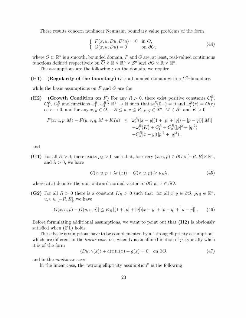
These results concern nonlinear Neumann boundary value problems of the formF (x, u,Du,D2u) = 0 in O,G(x, u,Du) = 0 on ∂O,

(44)

where O ⊂ Rn is a smooth, bounded domain, F and G are, at least, real-valued continuousfunctions defined respectively on O × R× Rn × Sn and ∂O × R× Rn.

The assumptions are the following : on the domain, we require

(H1) (Regularity of the boundary) O is a bounded domain with a C2–boundary.

while the basic assumptions on F and G are the

(H2) (Growth Condition on F ) For any R > 0, there exist positive constants CR1 ,

CR2 , CR

3 and functions ωR1 , ωR

2 : R+ → R such that ωR1 (0+) = 0 and ωR

2 (r) = O(r)as r → 0, and for any x, y ∈ O, −R ≤ u, v ≤ R, p, q ∈ Rn, M ∈ Sn and K > 0

F (x, u, p,M)− F (y, v, q,M +KId) ≤ ωR1 (|x− y|(1 + |p|+ |q|) + |p− q|)||M ||

+ωR2 (K) + CR

1 + CR2 (|p|2 + |q|2)

+CR3 |x− y|(|p|3 + |q|3) .

and

(G1) For all R > 0, there exists µR > 0 such that, for every (x, u, p) ∈ ∂O× [−R,R]×Rn,and λ > 0, we have

G(x, u, p+ λn(x))−G(x, u, p) ≥ µRλ , (45)

where n(x) denotes the unit outward normal vector to ∂O at x ∈ ∂O.

(G2) For all R > 0 there is a constant KR > 0 such that, for all x, y ∈ ∂O, p, q ∈ Rn,u, v ∈ [−R,R], we have

|G(x, u, p)−G(y, v, q)| ≤ KR [(1 + |p|+ |q|)|x− y|+ |p− q|+ |u− v|] . (46)

Before formulating additional assumptions, we want to point out that (H2) is obviouslysatisfied when (F1) holds.

These basic assumptions have to be complemented by a “strong ellipticity assumption”which are different in the linear case, i.e. when G is an affine function of p, typically whenit is of the form

〈Du, γ(x)〉+ a(x)u(x) + g(x) = 0 on ∂O. (47)

and in the nonlinear case.In the linear case, the “strong ellipticity assumption” is the following

23

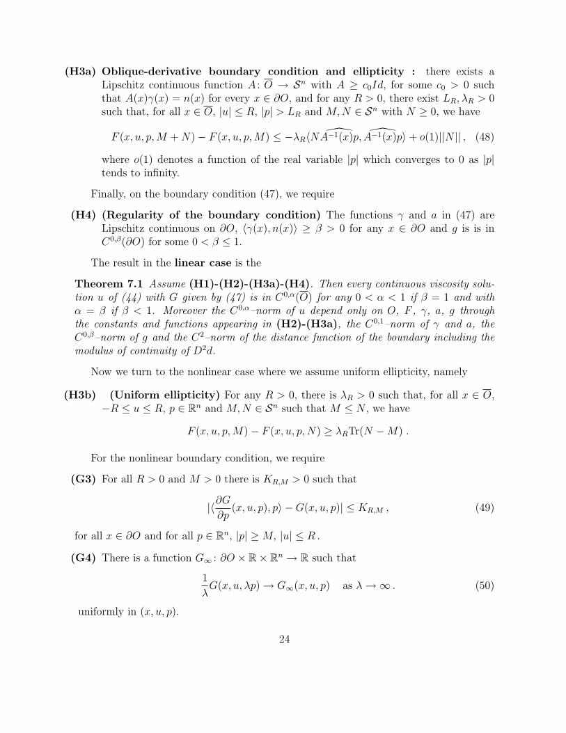
(H3a) Oblique-derivative boundary condition and ellipticity : there exists aLipschitz continuous function A : O → Sn with A ≥ c0Id, for some c0 > 0 suchthat A(x)γ(x) = n(x) for every x ∈ ∂O, and for any R > 0, there exist LR, λR > 0such that, for all x ∈ O, |u| ≤ R, |p| > LR and M,N ∈ Sn with N ≥ 0, we have

F (x, u, p,M +N)− F (x, u, p,M) ≤ −λR〈NA−1(x)p, A−1(x)p〉+ o(1)||N || , (48)

where o(1) denotes a function of the real variable |p| which converges to 0 as |p|tends to infinity.

Finally, on the boundary condition (47), we require

(H4) (Regularity of the boundary condition) The functions γ and a in (47) areLipschitz continuous on ∂O, 〈γ(x), n(x)〉 ≥ β > 0 for any x ∈ ∂O and g is is inC0,β(∂O) for some 0 < β ≤ 1.

The result in the linear case is the

Theorem 7.1 Assume (H1)-(H2)-(H3a)-(H4). Then every continuous viscosity solu-tion u of (44) with G given by (47) is in C0,α(O) for any 0 < α < 1 if β = 1 and withα = β if β < 1. Moreover the C0,α–norm of u depend only on O, F , γ, a, g throughthe constants and functions appearing in (H2)-(H3a), the C0,1–norm of γ and a, theC0,β–norm of g and the C2–norm of the distance function of the boundary including themodulus of continuity of D2d.

Now we turn to the nonlinear case where we assume uniform ellipticity, namely

(H3b) (Uniform ellipticity) For any R > 0, there is λR > 0 such that, for all x ∈ O,−R ≤ u ≤ R, p ∈ Rn and M,N ∈ Sn such that M ≤ N , we have

F (x, u, p,M)− F (x, u, p,N) ≥ λRTr(N −M) .

For the nonlinear boundary condition, we require

(G3) For all R > 0 and M > 0 there is KR,M > 0 such that

|〈∂G∂p

(x, u, p), p〉 −G(x, u, p)| ≤ KR,M , (49)

for all x ∈ ∂O and for all p ∈ Rn, |p| ≥M, |u| ≤ R .

(G4) There is a function G∞ : ∂O × R× Rn → R such that

1

λG(x, u, λp) → G∞(x, u, p) as λ→∞ . (50)

uniformly in (x, u, p).

24

The result in the nonlinear case is the

Theorem 7.2 Assume (H1)-(H2)-(H3b) and (G1)-(G4). Then every bounded con-tinuous solution u of (44) is in C0,α(O) for any 0 < α < 1. Moreover the C0,α–norm of udepend only on O, F , G, through the constants and functions appearing in (H2)-(H3b),and in (G1)-(G4), the C2–norm of the distance function of the boundary including themodulus of continuity of D2d.

Acknowledgements

The second author was partially supported by M.I.U.R., project “Viscosity, met-ric, and control theoretic methods for nonlinear partial differential equations” and byG.N.A.M.P.A, project “Equazioni alle derivate parziali e teoria del controllo”.

The authors wish to thank the anonymous referee for several valuable suggestionswhich allow them to improve the form of the article.

References

[1] Alvarez, O. & Bardi, M. : Viscosity solutions methods for singular perturbations indeterministic and stochastic control, SIAM J. Control Optim. 40 (2001/02), no. 4,1159-1188.

[2] Alvarez, O. & Bardi, M. : Singular perturbations of nonlinear degenerate parabolicPDEs: a general convergence result, Arch. Ration. Mech. Anal. 170 (2003), no. 1,17-61.

[3] Arisawa, M.: Ergodic problem for the Hamilton-Jacobi-Bellman equation. I. Exis-tence of the ergodic attractor, Ann. Inst. H. Poincar Anal. Non Linaire 14 (1997),no. 4, 415-438.

[4] Arisawa, M.: Ergodic problem for the Hamilton-Jacobi-Bellman equation. II. Ann.Inst. Poincare Anal. Non Lineaire 15 (1998), no. 1, 1-24.

[5] Arisawa, M.: Long time averaged reflection force and homogenization of oscillatingNeumann boundary conditions. Ann. Inst. H. Poincare Anal. Lineaire 20 (2003), no.2, 293-332.

[6] Arisawa, M. & Lions, P.-L.: On ergodic stochastic control, Comm. Partial Differ-ential Equations 23 (1998), no. 11-12, 2187-2217.

[7] Bagagiolo, F., Bardi, M. & Capuzzo Dolcetta, I. : A viscosity solutions approach tosome asymptotic problems in optimal control, Partial differential equation methodsin control and shape analysis (Pisa), 29-39, Lecture Notes in Pure and Appl. Math.,188, Dekker, New York, 1997.

25

[8] Bardi, M. & Da Lio, F.: On the strong maximum principle for fully nonlinear degen-erate elliptic equations, Arch. Math. (Basel) 73 (1999), no. 4, 276-285.

[9] Barles, G.: Solutions de viscosite des equations de Hamilton-Jacobi. Col-lection “Mathematiques et Applications” de la SMAI, n17, Springer-Verlag (1994).

[10] Barles, G. : Interior gradient bounds for the mean curvature equation by viscositysolutions methods, Differential Integral Equations 4 (1991), no. 2, 263-275.

[11] Barles, G.: Nonlinear Neumann Boundary Conditions for Quasilinear DegenerateElliptic Equations and Applications, Journal of Diff. Eqns., 154, 1999, 191-224.

[12] Barles, G. : & Da Lio F.: Local C0,α Estimates for Viscosity Solutions of Neumann-type Boundary Value Problems, preprint.

[13] Barles, G. & Lions, P.L.: Remarques sur les problemes de riflexion obliques, C. R.Acad. Sci. Paris, t. 320, Serie I, p. 69-74 (1995).

[14] Barles, G. & Ramaswamy, M.: Sufficient structure conditions for uniqueness of vis-cosity solutions of semilinear and quasilinear equations, to appear in NoDEA.

[15] Barles, G. & Souganidis, P. E.: On the large time behaviour of solutions of Hamilton-Jacobi equations, SIAM J. Math. Anal. 31, No.4, 925-939 (2000).

[16] Barles, G. & Souganidis, P. E. : Space-time periodic solutions and long-time behaviorof solutions to quasi-linear parabolic equations, SIAM J. Math. Anal. 32 (2001), no.6, 1311-1323

[17] Bensoussan, A. : Perturbation methods in optimal control, Translatedfrom the French by C. Tomson. Wiley/Gauthier-Villars Series in Modern AppliedMathematics. John Wiley & Sons, Ltd., Chichester; Gauthier-Villars, Montrouge,1988.

[18] Bensoussan, A. & Frehse, J.: On Bellman equations of ergodic control in Rn, J. ReineAngew. Math. 429 (1992), 125-160.

[19] Bensoussan, A. & Frehse, J.: Ergodic control Bellman equation with Neumannboundary conditions, Stochastic theory and control (Lawrence, KS, 2001), 59-71,Lecture Notes in Control and Inform. Sci., 280, Springer, Berlin, 2002.

[20] Bensoussan, A. & Frehse, J.: Regularity results for nonlinear elliptic systems andapplications, Applied Mathematical Sciences, 151. Springer-Verlag, Berlin, 2002.

[21] Capuzzo Dolcetta I. & Lions, P.L.: Hamilton-Jacobi equations with state constraints,Trans. Am. Math. Soc. 318 (1990), No.2, 643-683.

26

[22] Concordel, M.C.: Periodic homogenization of Hamilton-Jacobi equations: Additiveeigenvalues and variational formula, Indiana Univ. Math. J. 45, No.4, (1996), 1095-1117.

[23] Concordel, M.C.: Periodic homogenization of Hamilton-Jacobi equations: II: Eikonalequations. Proc. R. Soc. Edinb., Sect. A 127, No.4, (1997), 665-689.

[24] Crandall M.G., Ishii, H. and Lions, P.L.: User’s guide to viscosity solutions of secondorder Partial differential equations. Bull. Amer. Soc. 27 (1992), pp 1-67.

[25] Evans, Lawrence C.: The perturbed test function method for viscosity solutions ofnonlinear PDE, Proc. Roy. Soc. Edinburgh Sect. A 111 (1989), no. 3-4, 359-375.

[26] Evans, L. C.: Periodic homogenisation of certain fully nonlinear partial differentialequations, Proc. Roy. Soc. Edinburgh Sect. A 120 (1992), no. 3-4, 245-265.

[27] Evans, L. C. & Gomes, D.: Effective Hamiltonians and averaging for Hamiltoniandynamics. I., Arch. Ration. Mech. Anal. 157 (2001), no. 1, 1-33.

[28] Fathi A. : Theoreme KAM faible et theorie de Mather sur les systemes lagrangiens,C. R. Acad. Sci. Paris, Ser. I, 324 (1997), 1043-1046.

[29] Fathi A.: Solutions KAM faibles conjuguees et barrieres de Peierls, C. R. Acad. Sci.,Paris, Ser. I, Math. 325, No.6, (1997), 649-652.

[30] Fathi A.: Sur la convergence du semi-groupe de Lax-Oleinik, C. R. Acad. Sci., Paris,Ser. I, Math. 327, No.3, (1998), 267-270.

[31] Ishii, H.: Almost periodic homogenization of Hamilton-Jacobi equations, Interna-tional Conference on Differential Equations, Vol. 1, 2 (Berlin, 1999), 600-605, WorldSci. Publishing, River Edge, NJ, 2000.

[32] Ishii, H.: Perron’s method for Hamilton-Jacobi Equations, Duke Math. J. 55 (1987),369-384.

[33] Ishii,H.: Fully nonlinear oblique derivative problems for nonlinear second-order ellip-tic PDE’s, Duke Math. J. 62 (1991), 663-691.

[34] Ishii, H. & Lions, P.L. Viscosity solutions of fully nonlinear second-order ellipticpartial differential equations, J. Differ. Equations 83, (1990), No.1, 26-78.

[35] Lasry J.M. & P.L. Lions, P.L. : Nonlinear Elliptic Equations with Singular BoundaryConditions and Stochastic Control with State Constraints, Math. Ann. 283, 583-630(1989).

27

[36] Lions, P.-L.: Neumann type boundary conditions for Hamilton-Jacobi equations.Duke Math. J. 52 (1985), no. 4, 793-820.

[37] P.-L. Lions, G. Papanicolaou, S.R.S Varadhan, unpublished preprint.

[38] Lions P.L & Sznitman A.S, Stochastic differential equations with reflecting boundaryconditions, Comm. Pure and Applied Math. vol. XXXVII, pp 511-537, 1984.

[39] Namah G., J.-M. Roquejoffre, J.-M.: Remarks on the long time behaviour of thesolutions of Hamilton-Jacobi Equations, Commun. Partial Differ. Equations 24, No.5-6, 883-893 (1999).

28