Linear and Nonlinear PSE for Compressible Boundary Layers

NASA Contractor Report 191537cvJ-CD ICASE Report No. 93-70

ICASE ULINEAR AND NONLINEAR PSE FOR COMPRESSIBLE

BOUNDARY LAYERS

Chau-Lyan ChangMujeeb R. Malik

Gordon Erlebacher T)TICM. Yousuff Hussaini

D , C 2i 1

NASA Contract Nos. NAS 1-18605 and NAS 1-19480September 1993

Institute for Computer Applications in Science and EngineeringNASA Langley Research CenterHampton, Virginia 23681-0001

Operated by the Universities Space Research Association

S9-30649

National Aeronautics andSpace AdministrationLangley Research Center i 94Hampton, Virginia 23681-0001

ICASE Fluid Mechanics

Due to increasing research being conducted at ICASE in the field of fluid mechanics,

future ICASE reports in this area of research will be printed with a green cover. Applied

and numerical mathematics reports will have the familiar blue cover, while computer science

reports will have yellow covers. In all other aspects the reports will remain the same; in

particular, they will continue to be submitted to the appropriate journals or conferences for

formal publication.Accesion ForNTIS CRA&IDTIC TABU,,anrounced jJJ 'tii fc-ion

By ........... ...............................

--------------------------- - - ---------- -----------------

DItilP - I'

LTIC QhirY t,&EGTrfl 3

LINEAR AND NONLINEAR PSE FOR COMPRESSIBLEBOUNDARY LAYERS

Chau-Lyan Chang t and Mujeeb R. MaliktHigh Technology Corporation, P. 0. Boz 7262, Hampton, Virginia 23666

Gordon Erlebacher t and M. Yousuff HussainitICASE, NASA Langley Research Center, Virginia 23681-0001

Abstract

Compressible stability of growing boundary layers is studied by numericallysolving the partial differential equations under a parabolizing approximation. Theresulting parabolized stability equations (PSE) account for non-parallel as well asnonlinear effects. Evolution of disturbances in compressible flat-plate boundarylayers are studied for freestream Mach numbers ranging from 0 to 4.5. Results indi-cate that the effect of boundary-layer growth is important for linear disturbances.Nonlinear calculations are performed for various Mach numbers. Two-dimensionalnonlinear results using the PSE approach agree very well with those from direct nu-merical simulations using the full Navier-Stokes equations while the required com-putational time is less by an order of magnitude. Spatial simulations using PSEhave been carried out for both the fundamental and subharmonic type breakdownfor a Mach 1.6 boundary layer. The promising results obtained in this study showthat the PSE method is a powerful tool for studying boundary-layer instabilitiesand for predicting transition over a wide range of Mach numbers.

t This research was supported by NASA Langley Research Center under Contract NAS1-18240.

t This research was supported by the National Aeronautics and Space Administration under NASA Con-tract Nos. NASI-18605 and NASI-19480 while the authors were in residence at the Institute for Computer

Applications in Science and Engineering (ICASE), NASA Langley Research Center, Hampton, VA 23681.

ill..

I. Introduction

The subject of compressible boundary-layer stability has attracted a great dealof interest in the past few years due to its importance in understanding the on-set of transition in high-speed flows and providing some theoretical backgroundfor laminar flow control (LFC) techniques (Malik, 1990a). Most investigations ofcompressible linear stability (e.g., Mack, 1969, 1984) have employed what is knownas the "quasi-parallel" approach whereby the growth of the boundary layer is ig-nored and the linearized Navier-Stokes equations are reduced to ordinary differentialequations (ODE) by assuming a wave-like disturbance of the form

4 Y1 ~ (y)e(U+$ZWt) (1)

where x, y, and z are the streamwise, wall-normal, and spanwise coordinates, respec-tively; a and 0 are the corresponding wave numbers, w is the disturbance frequencyand %F represents the disturbance shape function. The linear ODE's along with thehomogeneous boundary conditions constitute an eigenvalue problem of the form

a = a(w, 0) (2)

which can be solved by standard eigenvalue techniques. The imaginary part ofa gives the disturbance growth rate and a small disturbance is expected to growprovided a, < 0. For a given flow, this eigenvalue approach can be applied "locally"at various locations along the body in order to obtain an idea about overall growthof disturbances and to correlate with transition location using empirical methodssuch as the eN method.

The effect of non-parallel flow on boundary-layer instability has been studiedby Gaster (1974), S.ric and Nayfeh (1975), Gaponov (1981), and El-Hady (1991).In the multiple-scales method used by the latter three authors, the disturbancesare decomposed into a slowly-varying shape function and a rapidly-oscillating wavepart. Both parts are represented as functions of a fast-scale variable (x) and a slow-scale variable (t = ex, with e = 1/R). With these assumptions the governing PDE'sare reduced to a set of ODE's by neglecting terms of order equal to or higher thane2 . In conjunction with the solvability condition, the analysis yields non-parallelcorrections to the eigenvalues computed by the quasi-parallel theory. Just like thetraditional linear theory, the multiple-scales approach can only be applied locallyfor a given problem.

Apart from the "local" methods described above, the evolution of disturbancesin a given flowfield may also be computed numerically by solving the governingpartial differential equations (PDE's) without resorting to the eigenvalue approach.The effect of boundary-layer growth and other history effects associated with ini-tial conditions and variation in wall temperature, for instance, can be properlyaccounted for. This was done for the G6rtler vortex problem by Hall (1983) and

1

Spall and Malik (1989). Denier et al. (1991) solved the "receptivity" problem toprovide the inflow conditions for the PDE's and were able to show how G6rtlervortex structure develops from a discrete roughness site.

The governing PDE's for the G6rtler problem are parabolic and thus the solu-tion can be obtained by direct marching provided the initial conditions are known.However, the governing equations for Tollmien-Schlichting (TS) and inviscid typedisturbances are elliptic and their solution cannot be obtained by simple march-ing methods. In addition, the numerical solution of these PDE's requires properoutflow boundary conditions which is a nontrivial task. However, we note that forboundary-layer type flows which are of interest here, the equation set is only weaklyelliptic along the dominant flow direction. Therefore, with appropriate simplifica-tions, one could "parabolize" these stability equations and avoid the difficultiesassociated with the downstream boundary conditions.

From a physical view point, the streamwise ellipticity arises from the upstreampropagation of acoustic waves and the streamwise viscous diffusion. To renderthe stability equations parabolic, one must devise a way to suppress, but withoutcompromising the essential physics, this upstream propagation. One way to derivethe parabolized stability equations (PSE) is to borrow ideas from the multiple-scalesapproach and decompose the disturbance into a rapidly-varying wave-like part and aslowly-varying shape function. The ellipticity is retained for the wave part while theparabolization is applied to the shape function. The resulting PSE can be solved bymarching along the streamwise direction. The technique can be used to study boththe linear and nonlinear evolution of convective disturbances in growing boundarylayers. Global or absolute instabilities can not be studied by this approach. Thisparabolizing procedure has been used recently by Bertolotti et al.(1992) for Blasiusflow.

The objective of this research is to study compressible boundary-layer stabilityand transition. We employ parabolized stability equations for linear and nonlin-ear development of disturbances in a compressible boundary layer. The nonlinearcalculations are carried all the way to the transition stage for supersonic flows. Insection II, we formulate the problem while the numerical procedure used to solvethe governing equations are given in section III. The results and conclusions arepresented in section IV and V, respectively.

II. Problem Formulation

The evolution of disturbances in compressible boundary layers is governed bythe compressible Navier-Stokes equations

+V(pV) = o

2

at + (V V)V] = -Vp + V[A(V • V)] + V- [/(VV + VET )] (3)

pep[ 5F + (V V)TJ = V.(kVT) + p + ( V)P+4

where V is the velocity vector, p the density, p the pressure, T the temperature, cpthe specific heat, k the thermal conductivity, p the first coefficient of viscosity, andA the second coefficient of viscosity. The viscous dissipation function is given as

A(V. f) 2 + L[VV + Vv T ]2.

2

The equation of state is given by the perfect gas relation

p = pRT

and the steady state solution of the basic flow can be derived by invoking theboundary-layer assumption.

In this research, we formulate the compressible stability problem in Cartesiancoordinates for the flat-plate geometry, although the theory itself can be easilyextended to axisymmetric bodies and infinite swept-wing flows. The Cartesiancoordinates are denoted by x, y, and z to represent the streamwise, wall-normal,and spanwise directions, respectively. All the lengths are scaled by a reference length1, velocity by ue, density by Pe, pressure by peu2, time by I/u,, and other variablesby the corresponding boundary-layer edge values. The basic flow is perturbed byfluctuations in the flow, i.e. the total field can be decomposed into a mean value(boundary-layer solution) and a perturbation quantity

u=ii+u', v=i+V', w=tf,+w'

p=i+p', p=A+p', T=T+T' (4)

A=pi+A', A=A+A', k=k+k'.

Substituting Eq.(4) into the Navier-Stokes equations given by Eq. (3) and sub-tracting from the governing equations corresponding to the steady mean flow, andusing the equation of state, we obtain the governing equations for the disturbancesas

04 __ __ __ 024 __2_ . 24r- + A-x !LO~ + C LO + D 0 = Vz,.x---- + V.u +xy '02'-YY

S +8O224 (5). 24~ 0__+ V -- +- V Y , 20• Y , 20.z Oyaz Oz2

where 4 contains the disturbance vector and is defined as

= (p', u', v', w', T') T .

3

Matrices r, A, B, C, D, V.., V2y, V1 y, V,., V., and V,, are Jacobians of thecorresponding total flux vectors and are composed of a linear part with only meanflow quantities (denoted by superscripts 1) and a nonlinear part which containsperturbation quantities (denoted by superscripts n): r = r' + rn, A = A' + A",etc. We note here that matrices r, A, B, C, D have contributions from both inviscid

and viscous terms, and thus contain terms of order one and of order 1/Ro (Ro isthe reference Reynolds number R 0 = uel/ve); while matrices Vz., V.., V.,, V,,V.,, V.,, and V.. are solely due to viscous diffusion and are of order l/R 0 .

To facilitate our discussion on the relation between linear and nonlinear dis-turbances, we rearrange Eq. (5) in the following form

!0€82 10 92¢t¢ 2 0€ ni02p1 9 Ž ~ V' OOk

Ot O-x4 AO+-y 4-C-z4-DO-Vz Ox2 VrP OOy "'Oy

axaz ayz IZ2(6)

where the left hand side contains only linear operators operating on the disturbance

vector and the right-hand-side forcing vector F" is due to nonlinear interaction andincludes all nonlinear terms associated with the disturbances. The right hand side

is given as

F" =n - r 00 A"n0 B ,0o -CnOt Ox Oy OzDn V 02¢ V 0 n20 n 02L

- " VO2 ,07"'- + Vy y (7)

+ V 0 + V" +2 V02SOO Z + y-- &-z2.

In the incompressible limit, F" contains quadratic nonlinearities; while, for com-pressible flows, cubic and higher-order nonlinearities are present. For small distur-bances, F" can be neglected and thus Eq. (6) reduces to the linearized Navier-Stokes

equations

r-+ A+B- +C B+D4+ON O'x TY OZ_-V1 ý 0¢ 1 90¢ y1 02€-V a20€

SVY - .OOz (8)

-1C) -v V 1 020 0

The governing PDE's of the disturbances, Equation (6), is hyperbolic in timefor the convection terms (inviscid part). When we consider only the spatial deriva-tives, Equation (6) is elliptic in the streamwise direction due to two reasons. First,the streamwise viscous term V,, allows any disturbances to be diffused upstream.

Second, and more importantly, the convection term in the streamwise direction

4

makes the upstream propagation of acoustic waves possible. The latter can be bet-ter understood by considering the linearized version of the inviscid equations andusing the method of characteristics (MOC) theory. Since the inviscid part of Eq.(8) is hyperbolic in time, the corresponding slopes of characteristic lines in the x - tplane (which determine the direction of propagation) can be found by solving thefollowing eigenvalue equation

JA' - A rli = 0.

Negative eigenvalues imply the wave is propagating from downstream to upstreamand vice versa. The eigenvalues of the above equation are

Ac= i ii, , + cif - C

where c is the speed of sound. For boundaxy-layer flows of interest in this study, thefirst four eigenvalues are always positive, while the last eigenvalue (fi - c) can beeither negative or positive depending upon the local Mach number (M, = a/c). Forsubsonic flows, this quantity is negative throughout the whole flowfield, therefore,the equation set (8), and thus (6), is elliptic. For supersonic flows, the ellipticityonly arises inside the subsonic layer adjacent to the wall.

Based upon the above discussion, one way to "parabolize" the PDE's given byEq. (6) and make the marching solution feasible is to neglect the viscous diffusionterms along the streamwise direction and prohibit the upstream wave propagationeither by dropping the left-running characteristics (associated with the eigenvaluei-c) (Chang and Merkle, 1989) or suppressing some part of the streamwise pressuregradient, as it is done in the Parabolized Navier-Stokes (PNS) approach (Vigneronet al., 1978). For the stability equations, the upstream wave propagation can besuppressed by either dropping the characteristic equation associated with the eigen-value ii - c or multiplying the streamwise pressure disturbance gradient Op'/9x bya parameter Q given by

fl = M. M, < 11 + (3- 1)M.2' (9)

=1, M, > 1

where - is the ratio of specific heats. These parabolizing procedures are quiteeffective for the PNS approach and yield solutions which compare favorably withthose obtained by the full Navier-Stokes equations provided a large portion of theflow is supersonic and only steady state solutions are of interest (Vigneron et al.,1978; Rubin, 1981). The advantage, of course, is the significant reduction in thecomputational cost due to the marching solution.

For compressible stability problems, the disturbances are essentially unsteadywaves propagating across the whole boundary layer and the amplitudes of these

5

waves reach their maxima near the critical layer located between the wall and theboundary-layer edge. These instability waves undergo a "fast oscillation" (phasechange) as they evolve along the flow direction. Direct application of the parab-olizing procedure used in the PNS approach for mean flow computations to ourgoverning stability equations would not capture the flow physics due to the sup-pression of the wave propagation along the left-running characteristics. Therefore,an alternative procedure must be devised.

Linear PSE

As mentioned previously, one way to "parabolize" the governing PDE's is tofirst decompose the disturbances into a fast-oscillatory wave part and a slowly-varying shape function. We keep the ellipticity for the wave part while parabolizingthe governing equation for the shape function. Following the lead of the non-parallellinear stability theory, we assume that the disturbance vector 0 for an instabilitywave with a frequency w and a spanwise wave number / (assume the wave is periodicin both the temporal and spanwise directions) can be expressed as

O(x,y,Z,t) = IP(x,y))e f:o a()d•+i5-,,) (10)

where i is the fast-scale variable, a(i) is the corresponding streamwise wave numberand 1P is the "shape function" vector given by

%p = (0, fi, 1, tij, ")T. (11)

As compared to Eq. (1), the shape function %P is now a function of both x and ydue to the growth of the boundary layer and the wave number a is a function of xto account for the growing boundary layer. For simplicity, we now restrict ourselvesto the linear case, i.e., only a single disturbance mode (w, 0) is considered and thenonlinear effect will be included later on. Substituting Eq. (10) into the linearstability equation (8), we have the following equation for the shape function

bi +bN =. +~• +VI,-• +,-, (12)OXZ~ ZUl OX gy PVYO2

where the vectors D, A and f are defined by

D= -iwr' + D' + iaA' + iC'

da 2)V'+ + afVh + #2V;'

? = A' - 2iaV' - iOV:

6

In the quasi-parallel linear theory where "normal-mode" analysis is employed,the shape function %P is assumed to be a function of y only (d'P/dx = 0); therefore,Equation (12) reduces to the following system of ODE's

LA = 0 (13)

where the operator L0 is given by

Lo =+ fd ddy YYdy 2

and the elements.of matrices n, d and are evaluated by assuming parallelmean flows (V = 0 and da/dx = 0). The above ODE's in conjunction with homoge-neous boundary conditions then constitute an eigenvalue problem described by thedispersion relation given in Eq. (2).

Unlike the normal-mode analysis described above, the decomposition (10) ex-hibits some extent of non-uniqueness between the distribution of the wave part andthe shape function part. In the PSE approach, we choose a complex wave num-ber a and construct a decomposition such that the change of shape function %Palong the streamwise direction x is of order 1/RO and the second derivative of IF(a 2 %p/4X2 ) is negligible. With this assumption and after neglecting all terms ofO(1/1R), Equation (12) reduces to

ft ft V, a2q-% + A + (14)4OX 9Y YY Oy2

Equation (14) describes the evolution of the shape function %P and is "nearly"parabolic in the sense that second derivatives in x are absent and the elliptic effectassociated with the wave part is absorbed in matrices D, A and B. For instance,the disturbance pressure gradient ap'•/ax, which is responsible for the upstreaminfluence, can be written as

apt ap qfZ cr(±t)dr+#z-wt)

a x ( iOq+ ± X ") e z-

The contribution of the wave part (iap3) is absorbed in the source term D'P and doesnot contribute to the upstream influence of the governing equations of the shapefunctions, Eq. (14). However, the pressure gradient shape function apl/ax associ-ated with the left-running characteristic (for subsonic flows only) is still present inthe x derivative term. The existence of this term allows upstream influence in Eq.(14). For stationary G6rtler vortex problem; a = 0 and aup/ax drops out, Eq. (14)reduces to the parabolic equations solved by Spall and Malik (1989).

For supersonic boundary layers, a large portion portion of the flow possessesonly downstream characteristics, our numerical results have shown that with a

7

properly chosen value of a (see discussion below) most of the upstream influenceis accounted for in iac3 and the elliptic effect associated with the pressure gradientshape function, Opl/&x, is negligible. To make Eq. (14) truly parabolic and enablea stable marching procedure for subsonic flows, we multiply 0i3/Ox by a constantQ defined in (9) (in the incompressible limit, this is equivalent to setting 'Op/axr tozero). While, this is formally true only in special cases (e.g. Gortler vortex problem),the approximation yields solutions which compare very well with accurate resultsfrom full Navier-Stokes equations (Joslin et al., 1992). This is because most of theellipticity is captured in the iac term.

For incompressible flows, one can use the vorticity-streamfunction formulationfor two-dimensional flows or use other formulations derived by eliminating the pres-sure from the momentum equations, as is done by Bertolotti et al. (1992). In theseapproaches, neglecting second and higher streamwise derivatives of the dependentvariables inherently suppresses some part of the streamwise pressure gradient, andconsequently prohibits the upstream propagation of information.

We now describe the strategy to update the streamwise wave number in or-der to make the marching scheme well-posed. The evolution of shape functions ismonitored during the process of marching and a is updated by local iterations at agiven x according to the change in T. The updating procedure is described herein.At a given location xi, we assume that the streamwise wave number is given by aland the total disturbance in the vicinity of x, can be expressed as

,(f¢(x,y,z,t) = I(x,y)e :1 •,dx+#z-,) (15)

The change of the shape function %P can be approximated by the following Taylorseries expansion truncated to the first order

%P(x,Y) = %P' + -i) + .

where 'P is the shape function at x = Xl. To an accuracy of O(x - xi), the aboveequation can be further expressed as

4,'(x,y) = Pje' 4 0dt (16)

Substituting (16) into (15), we have the "effective" wave number in the vicinity ofX, given by

1 d' 1a = ali T dx (17)

The real part of this effective wave number represents the phase change of thedisturbance while the imaginary part depicts the growth rate, both correspondingto the quantity %P chosen. A disturbance (%I') is unstable if the imaginary part

8

is less than zero. The updating procedure of a is repeated by using (17) until thechange in a is smaller than a prescribed tolerance (typically 10-12).

Since the shape function vector %P is a function of y and contains five depen-dent variables (A,fi, etc.), the updating procedure above is equivalent to choosinga normalization of the disturbance vector such that d'I l/dx is zero at a particulary location. Accordingly, the value of a computed by (17) will depend on the ycoordinate and the selected dependent variable TP1 . In this study, we have used theshape function fi (or i for compressible flows) at various y locations or the energyintegral (E = fo1 fil(2 + 62 + tb2 )dy), which is independent of the y coordinate,to update the wave number a and the resulting non-parallel growth rate (whichalso depends on the dependent variable and y coordinate chosen to measure thegrowth rate) appears to be very weakly dependent upon the normalization chosen(see discussion in section IV).

The solution of (14) requires proper boundary conditions in the wall-normaldirection. We apply the homogeneous Dirichlet conditions

fA=v= =T=0, y=0 (18)

at the wall and in the free-stream

fi - f - tb - 0, y --+-oo; (19)

although, these can be easily replaced by other conditions such as the Rankine-Hugoniot conditions at the shock (Chang et al., 1990) for supersonic flows. Non-homogeneous boundary conditions can also be imposed.

Nonlinear PSE

In the linear PSE approach described above, the disturbance amplitude is as-sumed to be infinitesimally small so that the nonlinear interaction of waves with dif-ferent frequencies and spanwise wave numbers is neglected. When finite-amplitudewaves are present in the flow, the linear approach is no longer valid. For nonlinearstudies, we assume that the total disturbance is again periodic in time and in thespanwise direction, thus, the total disturbance function € can be expressed by thefollowing Fourier series

00 00 i rý( ~ t jz- w)( 0Z Z o (20)

m--oo n--oo

where rmn and Tmn are the Fourier components of the streamwise wave number

and shape function corresponding to the Fourier mode (mw, nfl). The frequencyw and wave number # are chosen such that the longest period and wave length

9

are 2r/w and 2r/,6 in the temporal and spanwise domains, respectively. For moststability problems of interest, it is sufficient to truncate (20) to only a finite numberof modes

= �Z� Z '/.n(x,y)e' -m0¢k)d•+n•5-mwt (21)m=-M n=-N

where M and N are the total number of modes kept in the truncated Fourier series.For all nonlinear results presented in this study, we apply both the temporal andspanwise symmetry conditions whenever applicable, i.e., only one quarter of modes(m ranging from 0 to M and n ranging from 0 to N) are computed in the marchingprocess.

We now substitute Eq. (21) into our nonlinear governing equation (6) andperform harmonic balance (collect terms with the same spanwise wave number andfrequency) for both linear and nonlinear terms. The resulting governing equationsfor the shape function of a single Fourier mode (m, n) become

8'I'mn 8'Pmn_DmnImn + Amn.o__ + Bmn (22)

8Y Oy2 + Fmn/Amn

where matrices Dmn, Amn and Bmn are given by

Dmn = -imwr' + D' + iatmnA' + in#C'

(. damn. _2 + nam V1dx n c )v + n# z'

+ n2•V20

Amn = A' - 2ikmnVz' - ini6VhX zl

Bm, = B'- iamnV',, - in#V 1YX

and the quantity Amn is

Amn =e if-01 amn~tdt

The nonlinear forcing function Fi.n is the Fourier component of the total forcingdefined by Eq. (7) and can be evaluated by the Fourier series expansion of Fn

M N

F (x,y,z,t) = E E Fmn(x'y)e(",z-m"w)" (23)m=-M n=-N

The Fourier decomposition of Eq. (23) can be done by using the Fast FourierTransform (FFT) of F", which is evaluated numerically in the physical space. In

10

equation (22), a parabolizing procedure similar to that used in the linear PSE hasbeen employed in order to obtain a marching solution.

As in the linear PSE, the determination of the wave number amn plays animportant role in maintaining numerical stability. The procedure described abovefor computing a for linear disturbances can also be used for the determination ofamn. However, when all Fourier modes are nearly phase-locked (as is evident whenparametric resonance of secondary instability takes place, see e.g. Kachanov andLevchenko (1984)), one may assume that the wave number is given as

mn :-= (mnar, -- mn)

where a, is the real part of alo and amn denotes the growth rate of the mode (m, n).Each mode can have a different imaginary part am,, while the real part is updatedaccording to the phase change of the dominant fundamental mode. Additionalphase shifts in the harmonics are included in the evolution of the shape functions ofthe harmonic waves; therefore, all Fourier modes are not necessarily phase-locked.It needs to be pointed out that the "nearly" phase-locking assumption (since theevolution of shape functions may shift the phase slightly) mentioned above is usedfor convenience and is not necessary for the nonlinear analysis using PSE. In alater section, we will provide an example of a nonlinear calculation where we letthe disturbances evolve with and without the phase-locking rule. Use of the phase-locking rule, when applicable, saves computational cost.

The nonlinear PSE for a single Fourier mode, equation (22), is equivalent tothe linear PSE given in (14) with a frequency mw and a spanwise wave number nowith the addition of a forcing function. Since the forcing function acts as a "sourceterm" of the equation, the boundary conditions and solution procedure describedabove for the linear PSE can be directly applied to the nonlinear system, except forthe modes with zero frequency (m = 0). These zero frequency modes are denotedas the mean flow correction (if n = 0) or longitudinal vortex modes (if n # 0). Forthese modes, as in G6rtler vortex problem, the pressure gradient 9P1/Ox drops outmaking the equations fully parabolic.

The boundary conditions given in Eqs. (18) and (19) can be applied to thelongitudinal vortex mode without modification. For the mean flow correction, thefree-stream conditions are replaced by

- aboow00o= o00 = 00 = , y - 00 (24)

to account for the change of displacement thickness due to the correction of themean flow profile (it + fioo) arising from nonlinear interactions. This Neumanncondition for the normal velocity allows the mean flow given by the boundary-layersolution to adjust itself in order to assuire mass balance.

11

III Numerical Procedure

In this paper, we only consider the compressible stability of two-dimensionalboundary-layer flow past a flat plate. The mean flow solution is obtained by solv-ing the self-similar boundary layer equations. By using the Mangler-Levy-Leestransformation, the boundary-layer equations are transformed into a set of ordi-nary differential equations (ODE's). A fourth-order compact scheme is employed tosolve these ODE's. Details of the numerical procedures are given in Malik (1990b)and will not be repeated here.

Numerical solution of the parabolized stability equations (14) or (22) requiresdiscretization in both x and y directions. Since the boundary layer grows in thestreamwise direction, we expect that the solution for the shape functions will alsogrow. To ensure sufficient resolution as the disturbances evolve downstream, dis-cretization in the wall-normal direction must be able to account for the growth ofthe boundary layer. Instead of solving equations (14) and (22) in Cartesian coor-dinates, we transform these equations to a generalized coordinate system definedby

(X= y) (25)

in order to facilitate numerical computations on a "growing mesh" or curved wallgeometries. After this transformation, Equation (14) becomes

-84' -84'=•02ID'I + A -+B- + f3 - (26)

where the coefficient matrices are given by

D=D

A ,1 + v

2vtJ a7 Jj

The Jacobian of the transformation J is defined as

J = G77Y - G771.

Equation (22) can be transformed in a similar fashion.Using transformation (25), we map the computational grid into a uniform mesh

with constant increments in ý and 77 coordinates. For most of our calculations, weuse a constant step size in x while the grid is clustered near the wall to resolve therapid change inside the boundary layer. For high Mach number calculations, we also

12

cluster the grid near the critical layer located near the boundary-layer edge. Thestretching along the y direction is based on the local length scale I.. (l, = výi-l)which increases with the boundary-layer growth. The same grid distribution basedon y/I1 is used for all x locations while 1, increases with x.

We use indices i and j to denote the grid index along the streamwise (z) andwall-normal (y) directions, respectively. In the streamwise direction, we use thesecond-order backward difference

OT = (3P,,j - 4ki-',j + Pi-2,j)/2Aý

for all x locations, except for the starting plane where a first-order backward differ-ence is employed. The resulting discretized equation for the i-th streamwise planeis then 3 (9• ~0

[D + - A- + B - V=2Aý 5 a 2 (27)

A.•,(41F-•,j - Ti-2,j)/2Aý

In the wall-normal direction, we employ a fourth-order accurate finite-differencescheme. The two-point fourth-order scheme by Malik et al. (1982) is also used fornormal derivatives; however, it requires that the normal mean velocity T) is non-zeroand hence is not generally applicable for all problems.

For the uniform mesh in the ý - q plane, the normal derivatives in Eq. (26)are discretized according to the following fourth-order central difference formulae:

8a1' __ -T~ + 8IP i,j+l - 8%Pi,j- 1 +TiP,1 .. 2

877 12AY7

02 %a772-- -(-'Pi,j+2 + 16%Pi,j+l - 30%Pi,j

+ 16jj,.j- - Tij-2)/12A,2.

For the grid point next to the boundary, the above five-point scheme is replacedwith the second-order scheme

O'PS= ('Pj+1 - ,-)/A

02,

a -= ('i,j+l - 241ij + Qi,j-l)/2Ar72 .

At the boundary, five boundary conditions are needed for five dependent variablesin %F. The no-slip and free-stream boundary conditions given in (18) and (19)are used. In addition, we apply the discretized continuity equation as the fifthboundary condition both at the wall and the free-stream. Substituting the above

13

normal derivatives into (27) for all interior points and coupling with the boundaryconditions result in a block penta-diagonal system of equations at each x locationwith a block size of 5 x 5. This block matrix can be solved by the standard LUdecomposition method.

IV. Results and Discussion

To demonstrate the capability of the PSE approach, we perform both linearand nonlinear calculations for various Mach numbers. In the linear results, themain focus will be on the non-parallel effect, and in the nonlinear regime, PSEcalculations are carried all the way to the early stage of transition.

In the following discussion, we define the growth rate in non-parallel boundarylayers according to Eq. (17), i.e., for any given flow variable ik ( for instance, p, fi,etc.), the growth rate a is defined as

or = -Im(a) + Re(--). (28)0 OX

The second term on the right hand side of the above equation is a function of y;therefore, the growth rate in a non-parallel boundary layer depends upon the dis-tance normal to the wall. We note here that although Eqs. (17) and (28) are derivedbased on the same concept, they have different physical meanings. Briefly, Eq. (17)is used to normalize the disturbance vector and determine the wave number a. Foreach normalization, corresponding to different *I chosen in (17), the growth ratefor any given variable at any y location is to be evaluated using Eq. (28). For theresults presented herein, we compute the growth rate at the corresponding loca-tion where the fluctuation reaches its maximum value or based on the disturbancekinetic energy integral,

aE = -Im(a) + -•(lv'-E)lax

where E is defined byE = 10(fi2 +,b2 + tb2)dy

for the incompressible limit and by

E = I.(fi2 +±b2 + tb 2)dy

for general compressible flows. In supersonic wind tunnel experiments, the growthrate is usually measured for the mass flow fluctuation. We define the mass flowfluctuation as

(pu)' = p'ii + Au'. (29)

14

Linear PSE

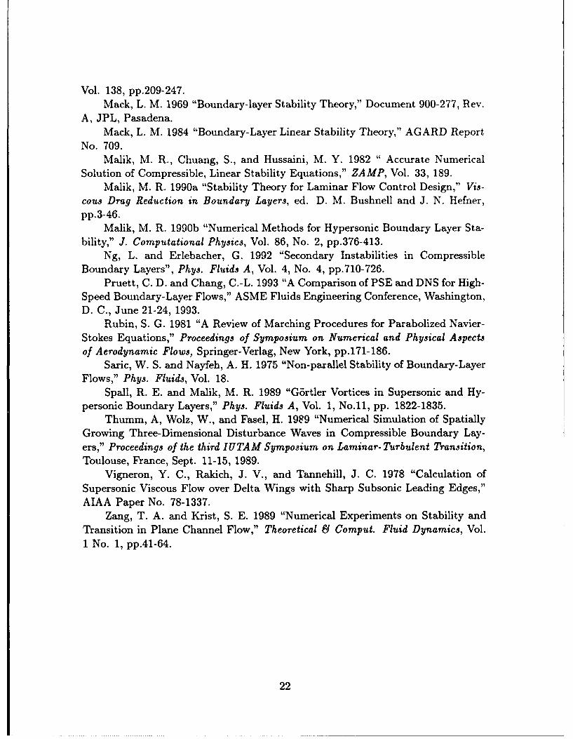
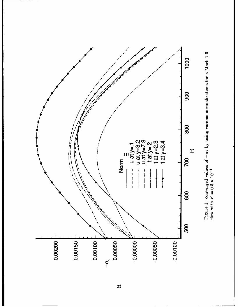
As mentioned in the previous section, the streamwise wave number a dependsupon the variable T, chosen and the y location where (17) is applied. To demon-strate that the resulting non-parallel growth rate is very weakly dependent uponvarious normalizations, we first perform calculations for a Mach 1.6 boundary layerby using different dependent variables to update a. These variables include fi, t(evaluated at various y locations as shown in the figure) and the kinetic energy inte-gral E defined above. Figure 1 shows the resulting imaginary part of the convergedvalue of a for the various norms. The results reveal that a strongly depends onthe norm chosen. -The corresponding effective growth rates ,,p, o'T and aE, eval-uated by using (28) at their maximum locations (for a'. and "T only) are shownin Fig. 2. It shows that the total growth rates depend on how they are measured(for instance, aT and aE are different); however, each non-parallel growth rate (e.g.apu) appears to be independent of the normalization procedure because results fromvarious norms collapse into one single curve. Similarly, although not shown here,the non-parallel wave number, evaluated by

10S= R e(a) - Im ag( -- ),

is also weakly dependent on the normalization. The above results indicate thatalthough different norms result in different values of a, the total growth rate (andwave number) by accounting for the evolution of shape function in the streamwisedirection remains the same regardless of the norms. For the results presented herein,we use the kinetic energy integral E in (17) to update a.

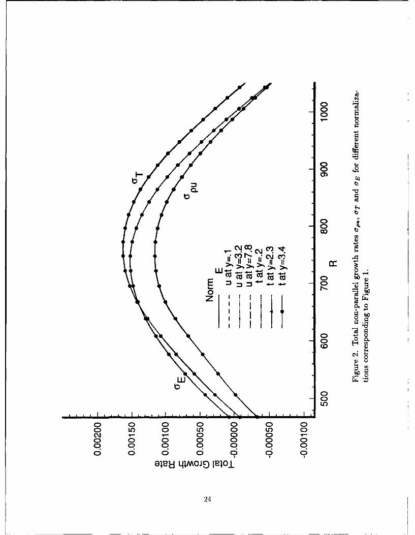
To verify the numerical algorithm, the first test case studied is an incom-pressible flow case. The incompressible results were obtained by choosing a Machnumber of 10-6 in our compressible formulation. Linear non-parallel results areavailable for incompressible boundary layer flow by using local methods from manyauthors(e.g., Gaster, 1974). The neutral points obtained from our PSE calcula-tions agree very well with thlose from Gaster's (1974) non-parallel method. Figure3 shows the computed variation of the growth rates (au, a,, and aE) with Reynolds

number (R = U/Z/ve) for a represen --'ive non-dimensional frequency (F = WR)of 1.12 x 10-4. The growth rates from multiple-scales method are shown by symbols.The results shown in Figure 3 reveal that the neutral curve near the upper branch isshifted to higher Reynolds numbers due to non-parallel effect as was found by Gaster(1974) and linear PSE results agree very well with those from the multiple-scalesapproach.

The second test case was chosen to be the Mac_ 1.6 case studied by El-Hady

(1991) using the multiple-scales ap.-, -ch. Ti,_ frequency was fixed at 0.4 x 10-4

and variable transport properties were used. Calculations were performed for both

15

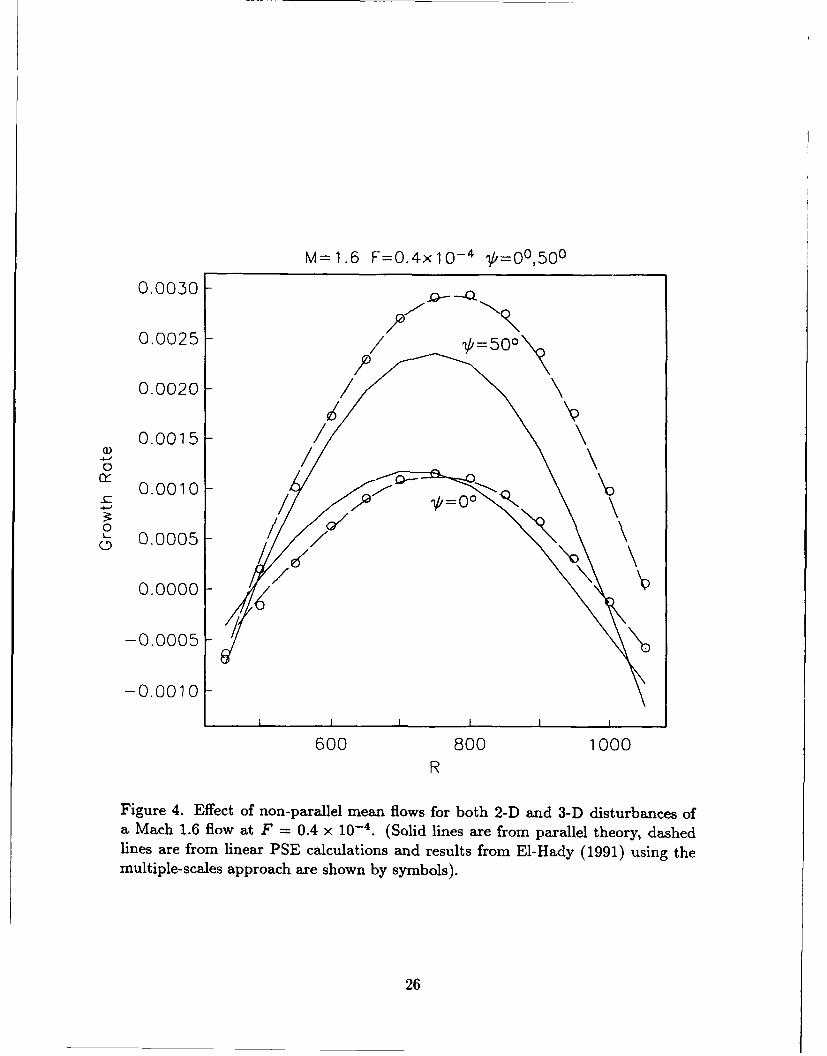
2-D and 3-D linear disturbances with an oblique wave angle of about 500 for thelatter. The growth rate of the mass flow fluctuations (defined in Eqs. (28) and(29)) from our PSE calculations together with the multiple-scales results are plottedalong with the growth rates obtained by quasi-parallel linear stability theory in Fig.4. Our PSE results agree quite well with those obtained from the multiple-scalesapproach. The results also indicate that for the first mode disturbance at Mach1.6, flow non-parallelism has more effect on three-dimensional disturbances thanon two-dimensional ones. Results obtained at higher Mach numbers also show anoticeable non-parallel effect on the first-mode instability.

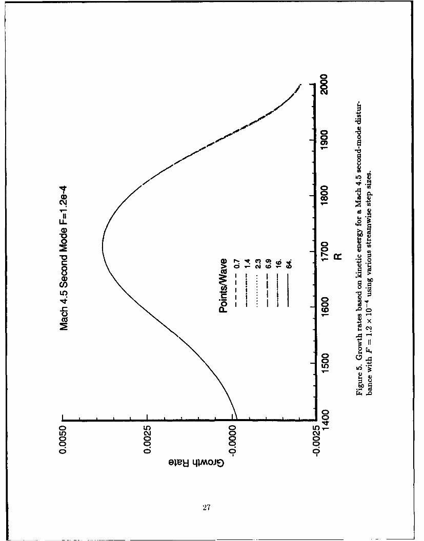
We now show some results for the Mach 4.5 flat-plate flow, which is subjectto second-mode instability (Mack 1984). Calculations were performed for a dis-turbance frequency of F = 1.2 x 10-4 with different streamwise resolutions. Weused step sizes ranging anywhere from 64 steps per wavelength to only one stepper wavelength. The results for the second-mode growth rate based upon the to-tal kinetic energy are plotted in Figure 5. There is essentially no difference in thegrowth rate results when two or more steps per wavelength are used. The reasonwhy only two points per wavelength could yield such accurate growth rates lies inthe fact that most of the wave information is absorbed in the complex wavenumbera. In contrast, direct numerical simulation (DNS) of Navier-Stokes equations wouldrequire many more points per wavelength for comparable accuracy.

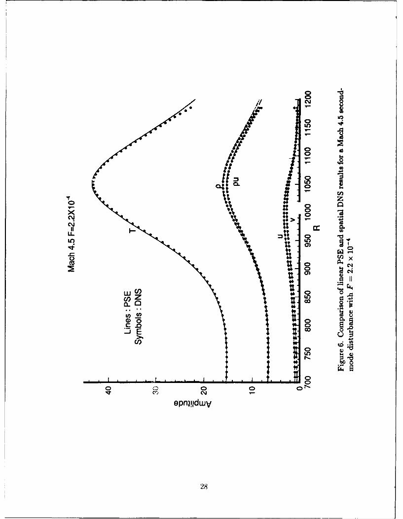
To further verify our linear results, we compare non-parallel evolution of asecond mode disturbance with a frequency of 2.2 x 10-4 with DNS. In Fig. 6,the maximum amplitudes of various flow quantities are plotted against Reynoldsnumbers for both PSE and DNS. The PSE results obtained by using only 7 stepsper wave length agree very well with DNS results using 16 steps per wave length.The PSE calculation took about 100 seconds CPU time while the DNS requiredmore than 40 hours on a Cray-YMP. Details of the comparison including nonlineardisturbances and the spatial DNS algorithm are given in Pruett and Chang (1993).

Nonlinear PSE

a. Computation of aIn a previous section we mentioned that the wavenumber a for the harmonics

may be determined either by the phase-locking rule or by using Eq. (17). It is knownthat the nonlinear wave interaction is dependent on the phase-difference betweenvarious modes. Therefore, it is essential that nonlinear PSE approach must notrequire phase-locking as a fundamental assumption; although, it may be used as aconvenience for problems where phase-locking happens anyway.

In order to demonstrate that phase-locking is not a basic assumption for non-linear PSE computations, the following test has been performed. Nonlinear calcula-tions have been done for a flat-plate boundary layer in the incompressible limit. Atwo-dimensional wave with a frequency F = .86 x 10' and an initial amplitude of

16

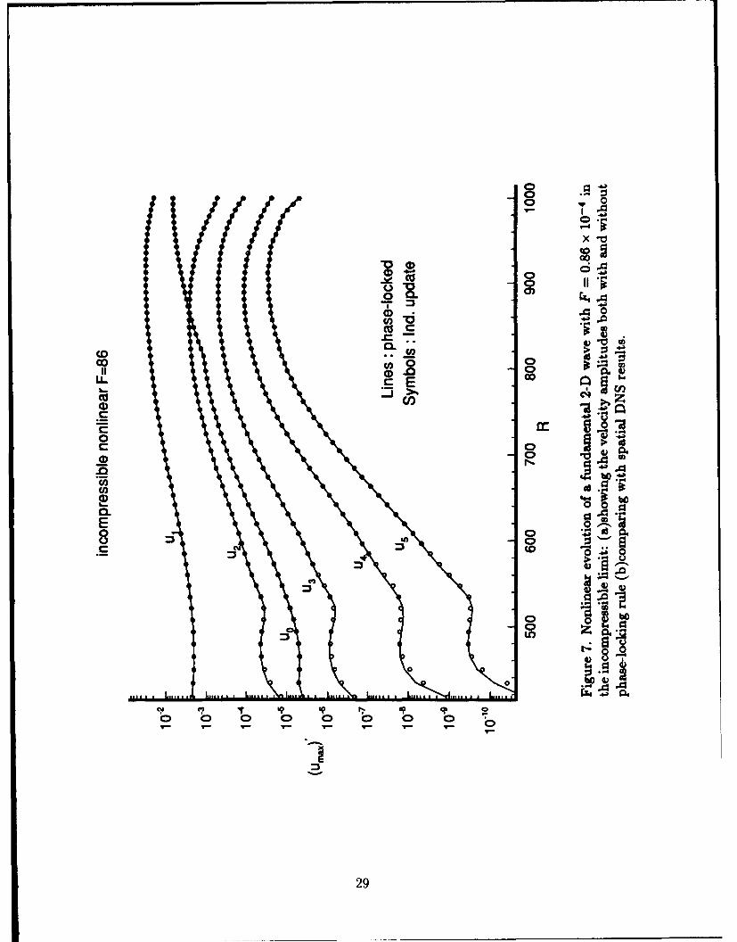
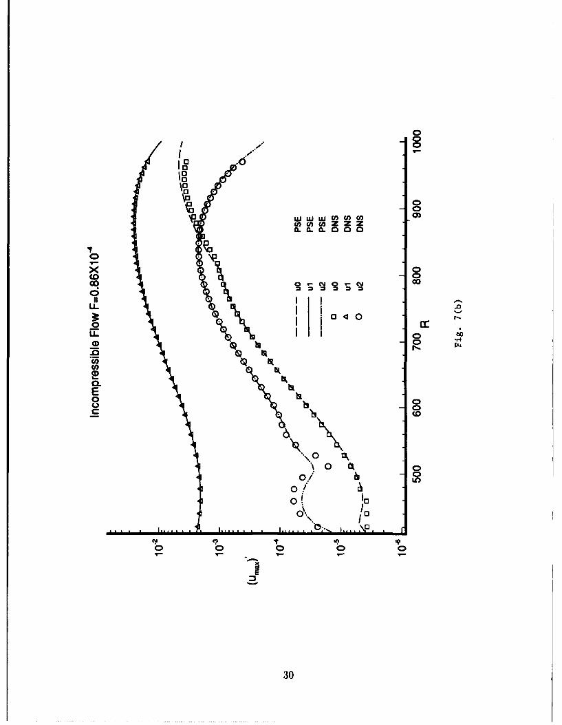
.25% at R = 400 is introduced in the boundary layer and the evolution of this wavealong with its various harmonics is monitored. Calculations were performed in twodifferent ways. First, the wavenumber a was computed for the fundamental waveaccording to Eq. (17) and the phase-locking rule was used for all the harmonics. Inthe second set of calculations, wavenumbers for the fundamental and all the harmon-ics were computed independently by using Eq. (17). The computed results for theamplitude of u velocity (fundamental, its four harmonics and meanflow correction)are presented in Fig. 7(a). It can be seen that only very minor differences appearbetween the two sets of calculations and these also tend to disappear as the calcu-lations are marched away from the inflow boundary. The second set of calculationstakes about 50% more computer time due to the iterations involved in determininga for the wave harmonics. Hence, it is expedient to use the phase-locking rule forproblems where this may be the outcome in any case.

In Fig. 7(b), the same nonlinear PSE results are compared with the spatialincompressible DNS results for fundamental, first harmonic and the mean flow dis-tortion modes. Both PSE and DNS start with the same initial conditions, i.e., a fun-damental disturbance (1, 0) at R = 400 and all harmonic waves including the meanflow distortion are generated through nonlinear interactions. The good agreementbetween DNS and nonlinear PSE indicates that the parabolizing approximation inthe PSE approach does not introduce any severe error and all detailed nonlinearfeatures are properly captured. Details of the comparison including disturbanceprofiles can be found in Joslin et al. (1992).b. Second-Mode Instability at Mach 4.5

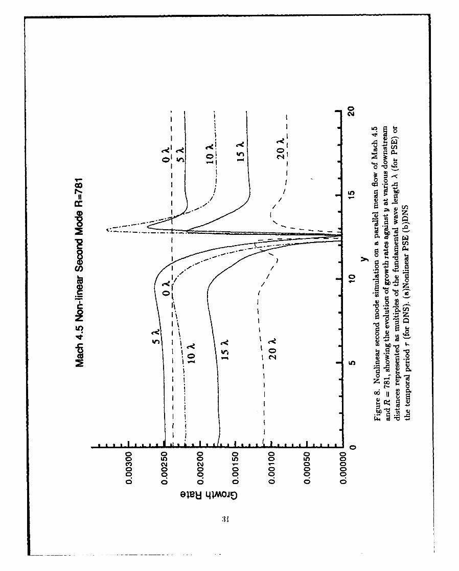
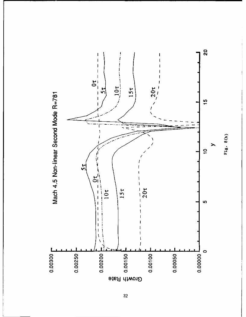
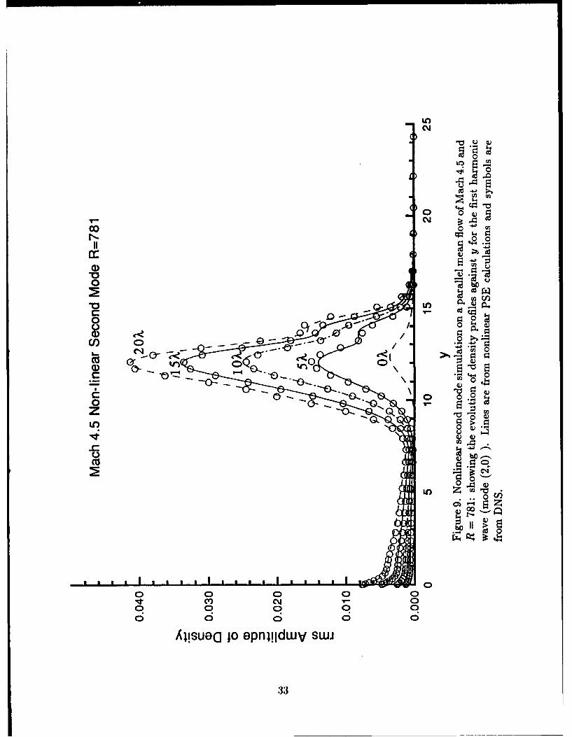
To verify the nonlinear PSE algorithm, we choose the nonlinear second modesimulation at Mach 4.5 investigated by Erlebacher and Hussaini (1990) using thetemporal DNS approach. As in the temporal DNS approach, we assume that themean flow is parallel and study the spatial evolution of disturbances in the presenceof nonlinear interactions. The initial conditions were provided by the eigensolutionfrom the linear theory at R = 781 and four Fourier modes (M = 3) were kept in thetruncated series. In our PSE calculation, the disturbance is assumed to be periodicin time and the nonlinear evolution is carried downstream in x as opposed to thetemporal DNS approach where the disturbance is periodic in x and integration iscarried in time. It was found in Erlebacher and Hussaini (1990) that due to non-linear effect, the growth rate of the fundamental disturbance strongly depends ony and there exists a sharp decrease in the local growth rate near the critical layer.The growth rates based on ill0 from our PSE results are shown in Figure 8(a) fordifferent x locations. The growth rate is initially uniform at the starting location(x = OA). As the disturbances are evolving downstream, r.cnlinear effects observedin Erlebacher and Hussaini (1990) are evident in the present spatial calculations.For comparison, their temporal DNS results are shown in Figure 8(b) at differenttime levels represented as multiples of the temporal period r. Figure 9 depicts theamplitudes of the density fluctuation of the first harmonic for both PSE calcula-

17

tions and the DNS results. The DNS results in Figure 9 are re-scaled to facilitatecomparison. Qualitatively, all nonlinear features observed in DNS, including thekink near the boundary-layer edge, are properly resolved in our PSE results.c. Subharmonic and Fundamental Resonance at Mach 1.6

Numerical simulation of incompressible flows have shown that the rapid growthof three-dimensional secondary disturbances is followed by breakdown to turbulence.Secondary instability is triggered when the primary disturbances reach sufficientlyhigh amplitudes. To show the capability of the PSE approach in simulating transi-tion onset, we also perform nonlinear calculations to study the secondary instabilitymechanism. We carry our calculations all the way to transition for both K-type (fun-damental) and H-type (subharmonic) breakdown. We choose Mach 1.6 flat plateflow with a primary disturbance frequency of 0.5 x 10-. The same flow conditionswere also used by Thumm et al. (1989) in their spatial Navier-Stokes simulationsof a compressible boundary layer.

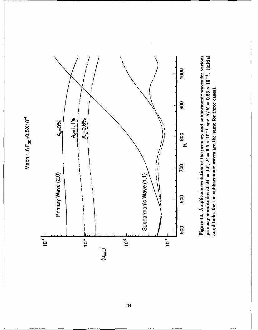
We first perform a series of calculations to determine the amplitude of theprimary disturbance which will trigger the secondary instability. The PSE calcu-lation is initiated at a Reynolds number R of 460 where we impose a primary 2-Dwave (mode (2, 0)) obtained by a local eigenvalue calculation and two subharmonicwaves ((1, 1) and (1, -1) modes) by using the compressible secondary instabilitytheory (Ng and Erlebacher, 1992) and all the remaining harmonics are assumed tohave zero amplitudes. Initial amplitudes of the primary disturbances are set to be3%, 1.1% and 0.6% at the inflow plane which corresponds to the 5%, 2% and 1%(the maximum amplitudes near the vibrating ribbon) cases given in Thumm et al.(1989). The initial amplitudes of the subharmonic waves are fixed at 0.019% forall three cases. The spanwise wave number of the subharmonic mode is fixed at13/R = 0.53 x 10-4 which corresponds to an oblique wave angle of 450. Six temporalFourier modes and three spanwise modes (M = 5 and N = 2) are kept in the Fourierseries. The evolution of both primary and subharmonic disturbances are shown inFigure 10. Qualitatively, our results agree with those of Thumm et al.(1989). Anyquantitative differences are due to different initial conditions. We find that a 1.1%initial amplitude (2% case in Thumm et al. (1989)) for the primary mode is enoughto trigger the secondary growth; however, the onset of secondary growth for thiscase occurs at R = 800 where the primary wave is about to decay. We continuethe PSE calculations beyond R = 1050 for this case and find that the secondarydisturbance eventually saturates and the flow does not reach the transitional stage.

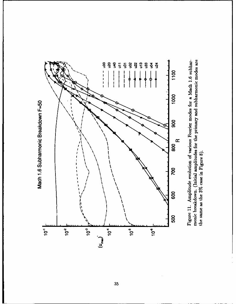
To carry the 3% case to the transition stage, we made another calculation withmore Fourier modes (M = 7 and N = 4) and the maximum velocity amplitudes ofsome representative modes are given in Figure 11. Besides the fundamental mode(2,0) and the subharmonic mode (1,1), higher harmonics in time and spanwisedomain are also excited due to nonlinear interaction. Initially, the (4, 0) mode gainsenergy from self-interaction of the (2, 0) mode and the interaction of (2, 0) and (1, 1)produces the (3, 1) mode. When the subharmonic mode grows due to the onset of

18

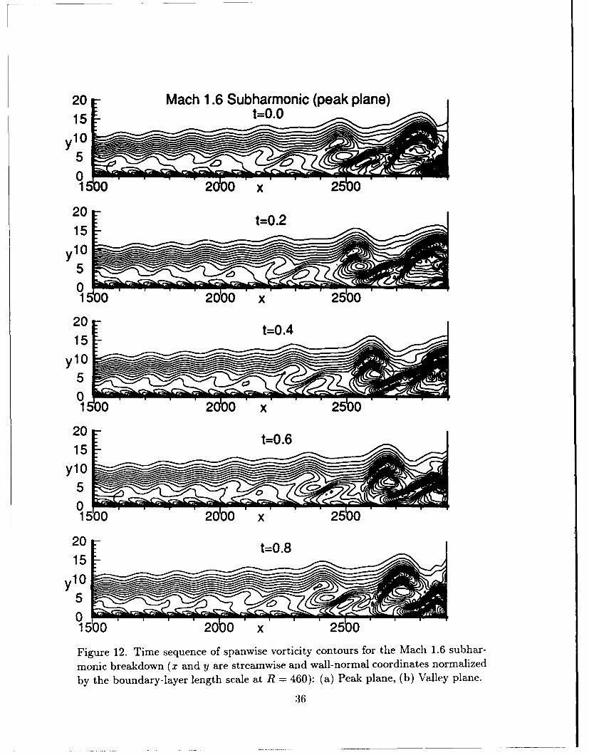
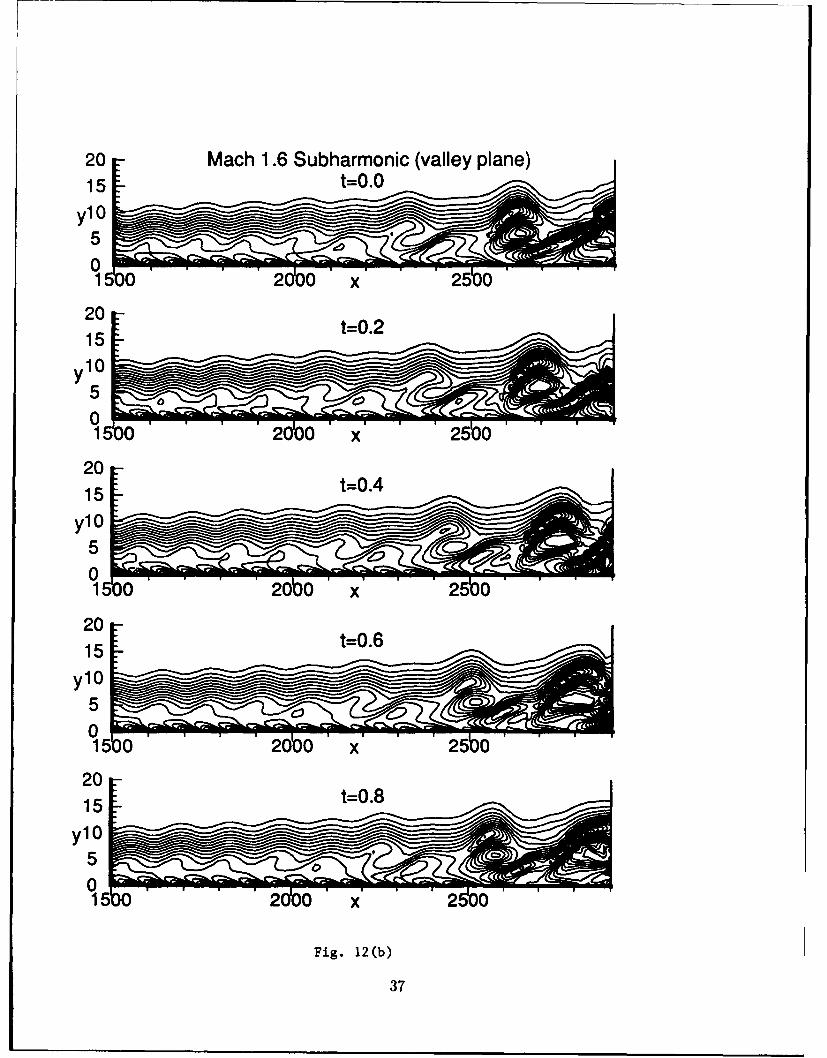
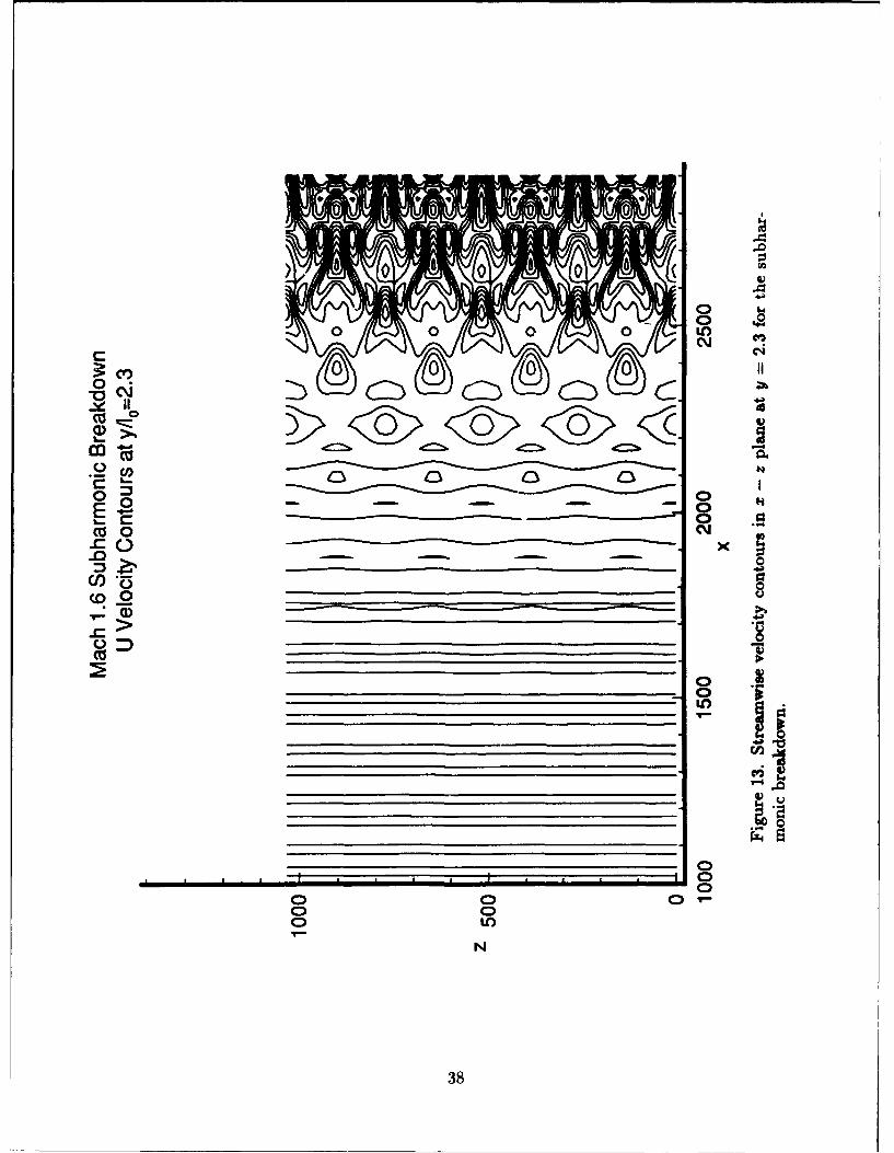
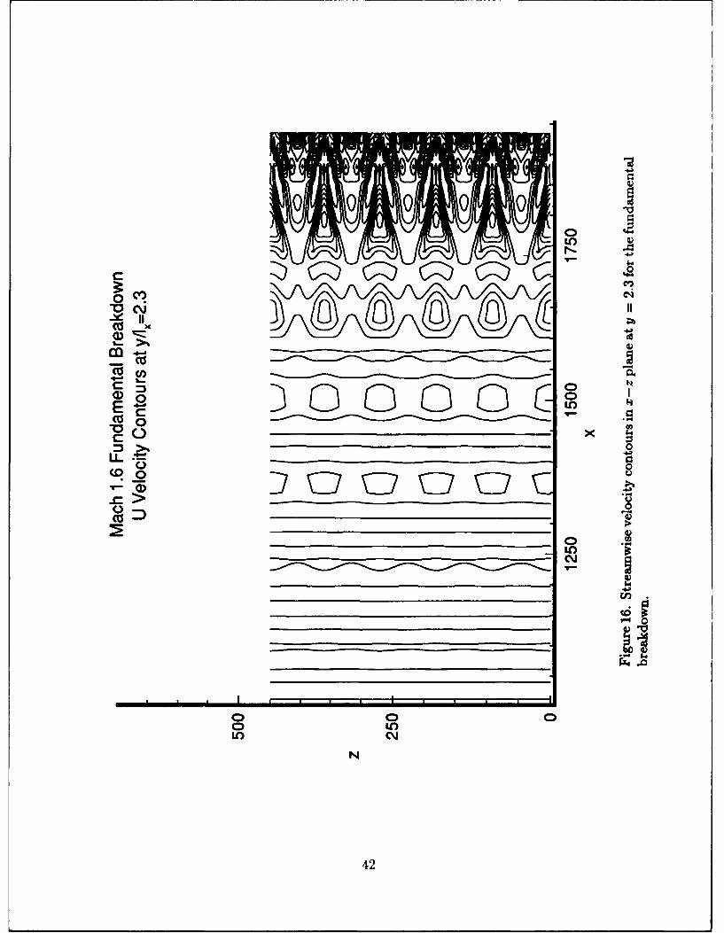
secondary instability, its harmonic (2,2) also grows at slightly higher rate. Thestreamwise vortex mode (0,2) arises due to the interaction of (1, 1) mode and itscomplex conjugate (-1, 1). As all these modes continue to grow, more and moremodes are excited. The energy cascade exhibits a staggered pattern. For instance,among the two-dimensional modes, only (2,0), (4,0), (6, 0), etc. gain energy; whilefor 1# modes, only (1, 1), (3,1), (5, 1), etc. are excited. The remaining modes (e.g.(1,0), (3,0), (0,1), (2, 1) etc.) remain unexcited throughout the calculation. Theabove staggered energy cascade is typical for subharmonic secondary instability.The secondary amplitude overtakes the primary at about R = 980 and reaches anequilibrium state around R = 1100. At this stage, many harmonic waves reachfairly high amplitudes as the flow heads for transition. We plot the time sequenceof spanwise vorticity contours at the peak and valley planes (corresponding to themaximum and minimum disturbance rms amplitudes, respectively) in Figures 12(a)and 12(b). As can be seen, the vorticity pattern doubles its wavelength for x >2200 (x is normalized w.r.t. the boundary layer length scale 1 at the initial plane)indicating the presence of high-amplitude subharmonic wave. It is also evidentthat the vortex roll-up results in a distinct kink in the shear layer. Towards theend of the computation, regions of intense vorticity near the wall begin to appearindicating that flow is heading for breakdown. Figure 13 shows the streamwisevelocity contours in the x-z plane for a wall normal distance of y = 2.3, where theTS wave reaches its maximum according to the linear solution. The flow is initiallytwo-dimensional and three-dimensional effect becomes important for x > 1800. Forx > 2000, a staggered contour pattern is evident. This pattern is associated withthe lambda vortex structure, a distinct characteristic of subharmonic breakdown,as observed in many incompressible experiments (e.g. Corke and Mangano (1989)).

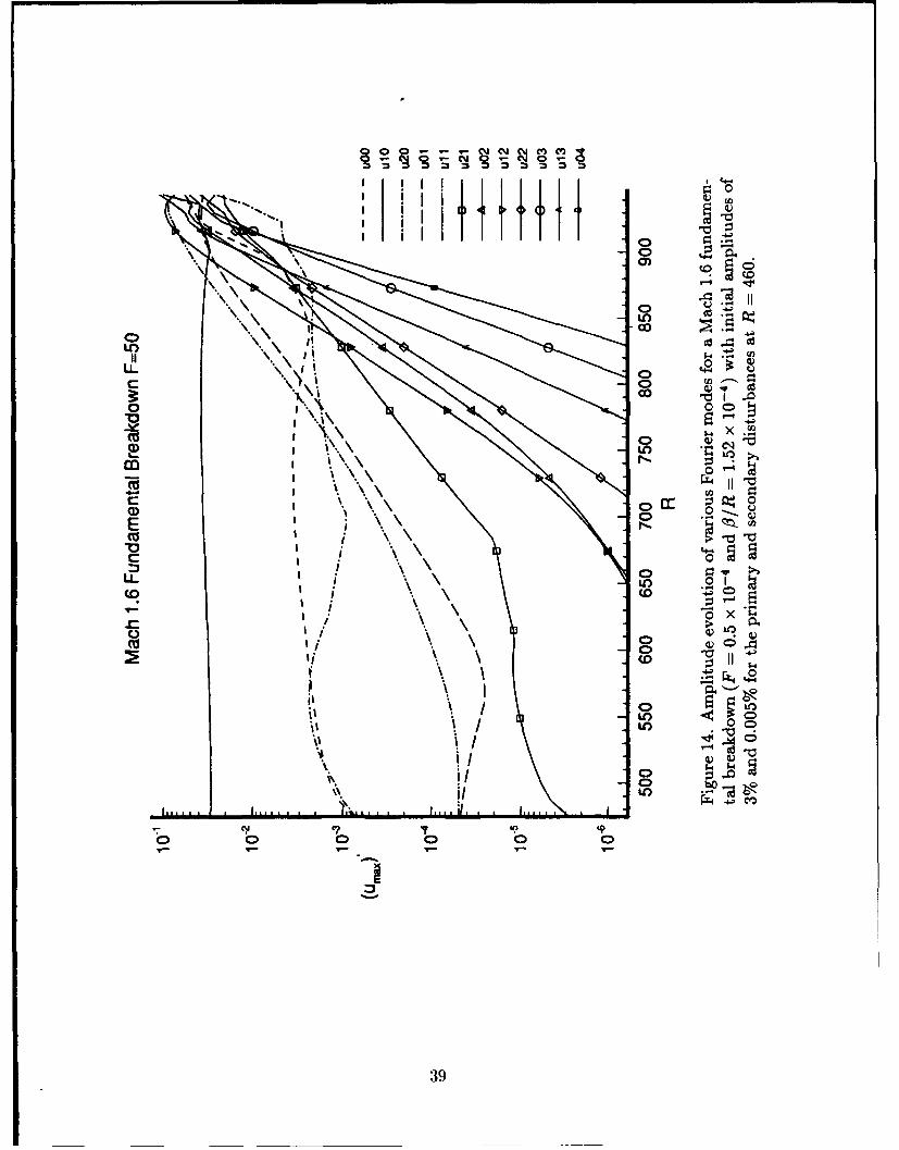
Nonlinear PSE calculations are also performed for the same Mach 1.6 case butfor a fundamental-type secondary resonance. The initial amplitude of the primarywave is again 3% and that of the secondary is taken to be 0.005% to minimizenonlinear interaction close to the starting location. The spanwise wave number isO/R = 1.52 x 10-4 (oblique wave angle of 600 for the secondary wave) and the pri-mary wave frequency is again 0.5 x 10-4. The initial conditions for our marching cal-culation consist of a 2-D primary wave (mode (1, 0)), two oblique fundamental-typesecondary disturbances (mode (1, 1), (1, -1)) and the longitudinal vortex (mode(0, 1)). The same number of Fourier modes as in the subharmonic case is used.

Nonlinear evolution of the maximum rms amplitude of u' is shown in Figure 14.Initially, the dominant modes are (1, 0), (1, 1), (0, 1) and (2, 0) (the first harmonic ofthe fundamental 2D mode). Unlike the subharmonic case, all harmonic waves (bothodd and even modes) gain energy directly from nonlinear interaction. Among them,the (2, 1) (due to (1, 0) and (1, 1)) and (1, 2) (due to (0, 1) and (1, 1)) modes aremore noticeable. For Reynolds numbers beyond 870, the spectrum is rapidly filledwith high-amplitude disturbances and the flow is heading towards transition. Ascompared to the subharmonic breakdown, transition location shifts upstream due

19

to the larger growth rate of the secondary disturbance as a consequence of higheroblique wave angle.

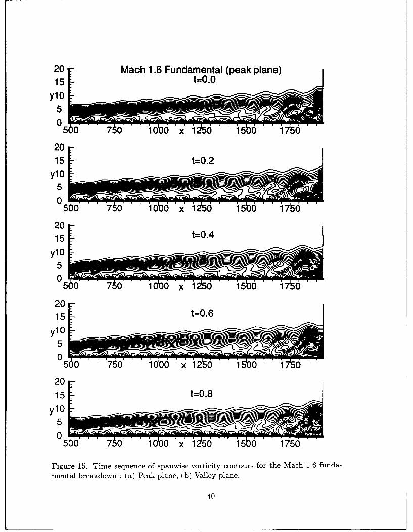
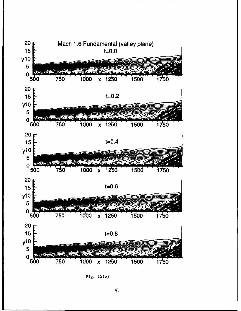
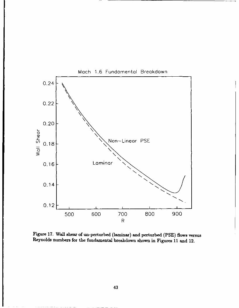
The time sequence of spanwise vorticity contours over a period of the primarywave is shown in Figures 15(a) and 15(b) for the peak and valley planes, respec-tively. In contrast to the subharmonic breakdoown, the wave length remains thesame throughout the whole computational domain. One important characteristic ofthe K-type breakdown is the appearance of aligned lambda vortices. This is bettervisualized in the streamwise velocity contours shown in Figure 16 for x > 1300.Similar to that observed in incompressible simulations of Zang and Krist (1989),regions of intense shear begin to appear near the end of the computational domainin Figures 15(a) and 15(b). This indicates that flow has just entered the transitionalstage. It is confirmed by plotting the average wall shear in Figure 17. The com-puted wall shear is slightly above the laminar value for most of the computationaldomain. Only towards the end, wall shear significantly departs from the laminarvalue indicating the onset of transition. In this way, PSE provides the predictionof boundary-layer transition for the imposed initial conditions. The PSE wall shearlies above the laminar value right from the beginning because of the relatively highamplitude of the 2-D primary disturbance needed for transition in supersonic flow.Since most amplified waves in supersonic flow are not two-dimensional, obliqueprimary modes may lead to transition for lower initial amplitudes. In order tocarry the calculations further into transitional regime, more spanwise and temporalresolution will be required. It remains to be seen how far PSE can proceed intothe transitional zone. The computational time used for the results presented inFigures 14-17 was 15 minutes on a Cray-YMP machine. Similar results from fullcompressible Navier-Stok-es equations would require 0(50) hours.

V. Conclusions

Linear and nonlinear compressible boundary-layer stability is studied by usingthe PSE approach. Several issues concerning the characteristics of the paraboliza-tion and the updating of the streamnwise wave number are also discussed. Thegoverning equations are solved by using second-order backward differences for thestreamwise derivatives while the wall-normal direction is discretized by a fourth-order accurate finite- difference scheme.

Non-parallel flow effects have been studied for linear disturbances. For obliquewaves of the first mode type, the departure from the parallel results is more pro-nounced as compared to that for the two-dimensional waves. Our linear results arein good agreement with those from the multiple-scales approach, as well as thosefrom full Navier-Stokes equations.

Nonlinear PSE calculations are carried all the way to the early stage of tran-sition for a Mach 1.6 flow. Both the subharmonic and fundamental types of break-

20

down are studied by the current PSE approach. Qualitatively, these breakdown

processes are similar to the ones in incompressible boundary layers, except that

high amplitudes of the 2-D primary wave are required. The promising results ofour PSE calculations show that this new approach is a powerful tool for the studyof boundary-layer stability and transition prediction. The parabolized form of thegoverning equations allow the numerical solution to be obtained in a computationaltime which is orders of magnitude lower than that required for direct simulation ofNavier-Stokes equations.

References

Bertolotti, F. P., Herbert, Th. and Spalart, P. R. 1992 "Linear and Nonlinearstability of the Blasius Boundary Layer," J. Fluid Mech., Vol. 242, pp. 4 4 1-4 74 .

Chang, C.-L., Malik, M. R., and Hussaini, M. Y. 1990 "Effects of Shock on theStability of Hypersonic Boundary Layers," AIAA Pdper No.90-1448.

Chang, C.-L. and Merkle, C. L. 1989 "The Relation between Flux Vector Split-ting and Parabolized Schemes," J. Computational Physics, Vol. 80, No. 2, pp.344-361.

Corke, T. C. and Mangano, R. A. 1989 "Resonant Growth of Three-dimensionalModes in Transitioning Blausius Boundary Layers," J. Fluid Mech., Vol. 209, pp.93-150.

Denier, J. P., Hall, P., and Seddougui, S. 0. 1991 "On the Receptivity Problemfor G6rtler Vortices and Vortex Motions Induced by Wall Roughness," Phil. Trans.R. Soc. Lond. A, 335, pp.51-85.

El-Hady, N. M. 1991 "Nonparallel Instability of Supersonic and HypersonicBoundary Layers," Phys. Fluids A, Vol. 3, No.9, pp. 2164-2178.

Erlebacher, G. and Hussaini, M. Y. 1990 "Numerical Experiments in SupersonicBoundary-Layer Stability," Phys. Fluids A, Vol.2 No.1, pp.94 -1 0 4 .

Gaponov, S. A. 1981 "The influence of Flow Non-Parallelism on DisturbanceDevelopment in the Supersonic Boundary Layers," Proceedings of the 8-th CanadianCongress of Applied Mechanics, pp. 673-674.

Gaster, M. 1974 "On the Effects of Boundary-Layer Growth on Flow Stability,"J. Fluid Mech., Vol. 66, pp.465-480.

Hall, P. 1983 "The Linear Development of Girtler Vortices in Growing Bound-ary Layers," J. Fluid Mech., Vol. 130, pp.4 1 -5 8 .

Joslin, R. D., Streett. C. L. and Chang, C.-L. 1992 "Validation of Three-Dimensional Incompressible Spatial Direct Numerical Simulation Code - A Compar-ison with Linear Stability and Parabolic Stability Equation Theories for Boundary-Layer Transition on a Flat Plate," NASA Technical Paper TP-3205.

Kachanov, Y. S. and Levchenko, V. Y. 1984 "The Resonant interaction ofdisturbances at Laminar-turbulent transition in a Boundary Layer," J. Fluid Mech.,

21

Vol. 138, pp.209-247.Mack, L. M. 1969 "Boundary-layer Stability Theory," Document 900-277, Rev.

A, JPL, Pasadena.Mack, L. M. 1984 "Boundary-Layer Linear Stability Theory," AGARD Report

No. 709.Malik, M. R., Chuang, S., and Hussaini, M. Y. 1982 " Accurate Numerical

Solution of Compressible, Linear Stability Equations," ZAMP, Vol. 33, 189.Malik, M. R. 1990a "Stability Theory for Laminar Flow Control Design," Vis-

cous Drag Reduction in Boundary Layers, ed. D. M. Bushnell and J. N. Hefner,pp.3-46.

Malik, M. R. 1990b "Numerical Methods for Hypersonic Boundary Layer Sta-bility," J. Computational Physics, Vol. 86, No. 2, pp. 3 7 6-4 1 3 .

Ng, L. and Erlebacher, G. 1992 "Secondary Instabilities in CompressibleBoundary Layers", Phys. Fluids A, Vol. 4, No. 4, pp. 7 10 -72 6 .

Pruett, C. D. and Chang, C.-L. 1993 "A Comparison of PSE and DNS for High-Speed Boundary-Layer Flows," ASME Fluids Engineering Conference, Washington,D. C., June 21-24, 1993.

Rubin, S. G. 1981 "A Review of Marching Procedures for Parabolized Navier-Stokes Equations," Proceedings of Symposium on Numerical and Physical Aspectsof Aerodynamic Flows, Springer-Verlag, New York, pp.171-186.

Saric, W. S. and Nayfeh, A. H. 1975 "Non-parallel Stability of Boundary-LayerFlows," Phys. Fluids, Vol. 18.

Spall, R. E. and Malik, M. R. 1989 "G6rtler Vortices in Supersonic and Hy-personic Boundary Layers," Phys. Fluids A, Vol. 1, No.11, pp. 1822-1835.

Thumm, A, Wolz, W., and Fasel, H. 19?9 "Numerical Simulation of SpatiallyGrowing Three-Dimensional Disturbance Waves in Compressible Boundary Lay-ers," Proceedings of the third IUTAM Symposium on Laminar- Turbulent Transition,Toulouse, France, Sept. 11-15, 1989.

Vigneron, Y. C., Rakich, J. V., and Tannehill, J. C. 1978 "Calculation ofSupersonic Viscous Flow over Delta Wings with Sharp Subsonic Leading Edges,"AIAA Paper No. 78-1337.

Zang, T. A. and Krist, S. E. 1989 "Numerical Experiments on Stability andTransition in Plane Channel Flow," Theoretical & Comput. Fluid Dynamics, Vol.1 No. 1, pp.4 1-6 4 .

22

v /

- 0I C

/ 0

/, 0

0)

C C>

/1 / coim .o 0

00

C)~ 0(0

0O 0

C)C)-

\L

o 0 0 C0 0 0) 0C'J 0 0 0) Co; 0 0 0) 0D 0= 0

231

Co0)Co

0

C)k

o) a..

o0

co b

C~j 00cl.4q:

Ec

N-0'!I! II

C) 0

0$-4

000

C)

C>J 0 0 0 1

o 0 0 0 a 0-0 0 0 0 a C00C 0 0 0 0) 0

918 L41MOJE) IIoZ

24

0

0f 0

Oil0

E0 0

CDD

oO

4WX

WWW CCfLO C

I ~ IIole !iIjE

o2

M=1.6 F=0.4x 10V4 =0 0 ,50 0

0.0030 F --- a

0.0025 =500

0.0020-

0.0015-

ry 0.00 10-

S/0.0005

0.0000-

-0.0005

-0.0010

II I I I I

600 800 1000R

Figure 4. Effect of non-parallel mean flows for both 2-D and 3-D disturbances ofa Mach 1.6 flow at F = 0.4 x 10-4. (Solid lines are from parallel theory, dashedlines are from linear PSE calculations and results from El-Hady (1991) using themultiple-scales approach are shown by symbols).

26

1.00

co

0 C))

8L 0 1

CO o

CC

LOO U'j)1

C; Ii I I0..e (0mjE

o2

8

0

Ii)

t a:

LL 0

CTS* 0 C

0-

LLJ 0

0 0.~J. C\EpnlGow

U28

V00

CCO

ob

EC

00

C) C

02

I k 0

CLC .0 0 0 a

x0coi

0

0 000

0 00

E h 0

1 10

C 30

00

0

00oo . -

4g

Co 4) 4

Ii I AR

Iiz

Ii -

I II

00

CO 0Y 0 00

o~C 0 0;

ejeld 41vo~JE

.: I

co cl0

00

co I I/- 1

C) C)0C)C

0;C iC

eVl ~oE

:3

0 . "

0

0.

00

C.))0 0

91 0

-00

(1)

0 0

C.Cc

Cu -

C13 0 C"'

00o0 4 0 0

o00 0 0

Aiisue] lo epnliidwV swi

33

d x

I0

LfI IN

0>

00

%- E

0- 0

0o.

C? If

CDu

34 -

* i 0)Qi%

oo

ILL-

\ -o

a)a

o 0

CI It 0

-9 ItIt (

II S/I *

I; \0 . .

S 0 0 0 0 0

35

20 Mach 1.6 Subharmonic (peak plane)15 N0.0

y0501 0 20b0 x 2500

2015

Y10501 0 2C00 x 2500

20-15

Y105

1200 x 25020-20 t=0.615

Y 1 .. .... ... ... --

50&A

S200 x 2500

2015

Y10501 15o200O x 250o

Figure 12. Time sequence of spanwise vorticity contours for the Mach 1.6 subhar-

monic breakdown (x and y are streamwise and wall-normal coordinates normalizedby the boundary-layer length scale at R = 460): (a) Peak plane, (b) Valley plane.

36

20 Mach 1 .6 Subharmonic (valley plane)15t=0

Y 15

20

15

Yb5

1 0 200 x 2b

2015t=.

5

100200o x 250o

2015t=.

5

10200o x' 250o

2015NO

Y10

5

Fig. 12 (b)

37

Ifr)

c C~j cN

ýt 0 0 0 1

-CD.2O co_

c : _ _ _ _ _ _ _ _ _ _ _ _ _ _ _ _ _

E_ _ _ _ _ _ _ _

Z:, 0

0 00 Dt

co~

N

38

IIC)

oor

LL a 0

00

LC

0

(U ~O0

CC

CDD

00

It 'I' \ I6

\ hIC'I

Ci

39

20 Mach 1.6 Fundamental (peak plane)15 t=0.0

Y 15

05 0 7!0 1000 x 120 1500 150

2015 t=0.2

ylO5 0

05 0 760 1000 x 10 1500 150

2015 t=0.4

Y1505 0 170 i x 1250 1500 150

2015 t=0.6

Y105050 70 1000 x 1250 5b0 150

2015 t=0.8

5

05660 7t'0 1000 x'1250 150 150

Figure 15. Time sequence of spanwise vorticity contours for the Mach 1.6 funda-

mental breakdown : (a) Peak plane, (b) Valley plane.

40

20 Mach 1.6 Fundamental (valley plane)15 t=0.0

YlO5Ln0

50 70 100 x' 120 1530 1

2015 t=0.2

ylO

05i070 1F0 X 125 50 170

2015 t=0.4

YlO5

20 0 0 7!0 100 Xl 0 150 150

20-

15 t=0.6ylO0

5050 70 10. 0 x' 1ý50 1500 7 0

2015. t=0.815

Ybb

005,0 "70 10x 150 1 506 150

Fig. 15 (b)

41

LO 4)

4a

00

cd

V)V C."

0C\J N

Cu )(42

Mach 1.6 Fundamental Breakdown

0.24 -

0.22

0.20

0Q)C- 8 Non-Linear PSEL 0.18 -

0

0.16- LaminarN

0.14IN

0.12 -

500 600 700 800 900R

Figure 17. Wall shear of un-perturbed (laminar) and perturbed (PSE) flows versusReynolds numbers for the fundamental breakdown shown in Figures 11 and 12.

43

REPORT DOCUMENTATION PAGE F or AAE-OW

gather~~~~~~~~~~~~~~~~~nq~~~~ ud inghg h aaneed n Oe~fgMdr~~l9tw(dt~ Ofe flow,~t01 ford r~tn etl;h.Jd n strtb~bad . searc"t O it a n g dVffaeta wof th

Collection Of Information. including S4q to m .0oS to' "'I"C t'I" burdenl to We"Uqto" 6 ine901 ftlet v etcei. Ditftorrye fo 1 41n om oon erif,.of And ftepofl. 1211 ieffenoDamt Highwel. S~l IM0. Athtlg=, VA 22024302, &W to the office. of Mana qvont and 5~d.e PapWWr emeot R nPlop" (0?04-OIUW),Watfurviton. DC 20103

I. AGENCY USE ONLY (Lavaie biank) 2. REPORT DATE -. REPORT TYPE AND DATES COVERED

C) 93 Cntr~tnrRavnnrt4. TTLE ND UBTILE5. FUNDING NUMBERS

LINEAR AND NONLINEAR PSE FOR COMPRESSIBLE BOUNDARY LAYERS C NASI-18605C NAS1-19480

AWHOR(S)WU 505-90-52-01

7. PERFORMING ORGANIZATION NAME(S) AND ADDRESS(ES) B. PERFORMING ORGANIZATION

Institute for Computer Applications in Science REPORT NUMBERand Engineering ICASE Report No. 93-70

Mail Stop 132C, NASA Langley Research CenterHampton, VA 23681-0001

2. SPONSORING / MONITORING AGENCY NAME(S) AND ADORESS(ES) 10. SPONSORING/I MONITORINGNational Aeronautics and Space Administration AGENCY REPORT NUMBER

Langley Research Center NASA CR-191537Hampton, VA 23681-0001 ICASE Report No. 93-70

III. SUPPLEMENTARY NOTES

Langley Technical Monitor: Michael F. CardFinal Report

12a. DISTRIBUTION /AVAILABILITY STATEMENT 1 2b. DISTRIBUTION CODE

Unclassified - UnlimitedI

Subject Category 341

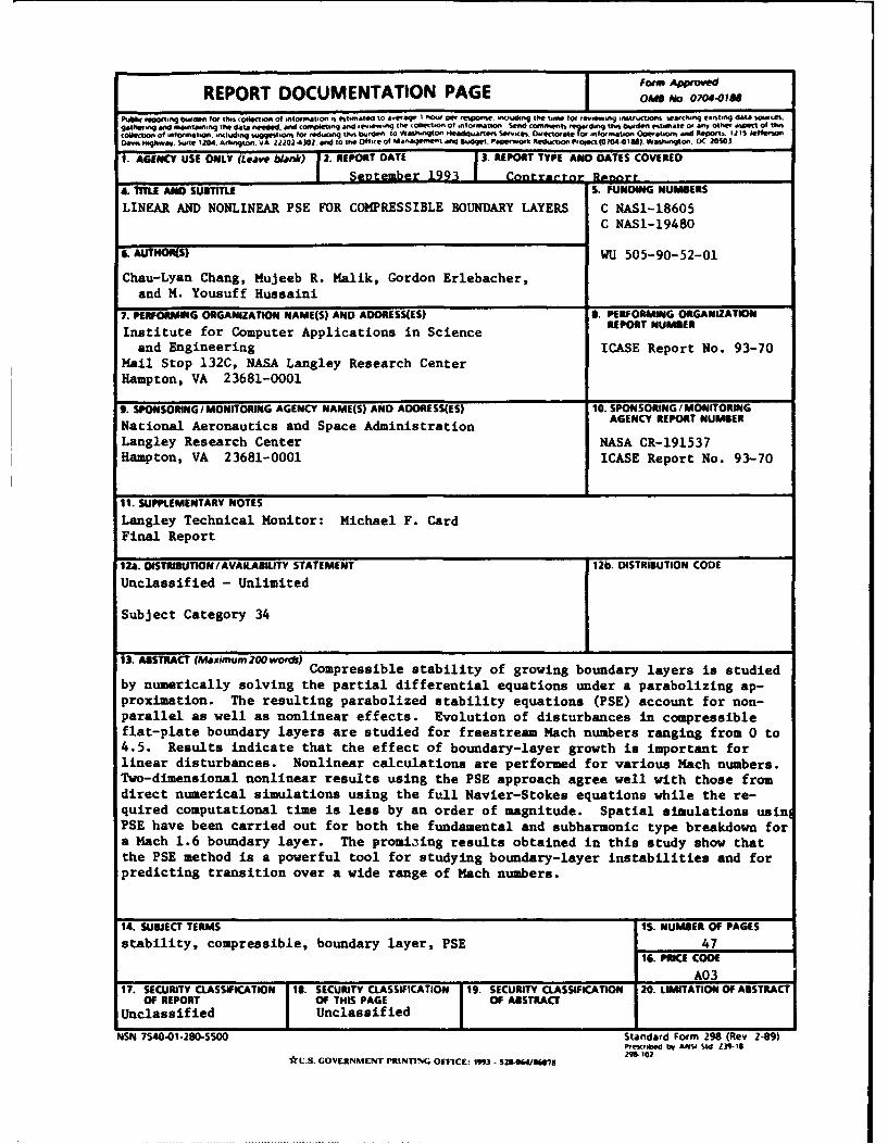
13. ABSTRACT (Maximum 200 words) Compressible stability of growing boundary layers is studied

by numerically solving the partial differential equations under a parabolizing ap-proximation. The resulting parabolized stability equations (PSE) account for non-parallel as well as nonlinear effects. Evolution of disturbances in compressibleflat-plate boundary layers are studied for freestream Mach numbers ranging from 0 to4.5. Results indicate that the effect of boundary-layer growth is important forlinear disturbances. Nonlinear calculations are performed for various Mach numbers.Two-dimensional nonlinear results using the PSE approach agree well with those fromdirect numerical simulations using the full Navier-Stokes equations while the re-quired computational time is less by an order of magnitude. Spatial simulations usinPSE have been carried out for both the fundamental and subharmonic type breakdown fora Mach 1.6 boundary layer. The promi3ing results obtained in this study show thatthe PSE method is a powerful tool for studying boundary-layer instabilities and forpredicting transition over a wide range of Mach numbers.

14. SUBJECT TERMS IS. NUMBER OF PAGES

stability, compressible, boundary layer, PSE 4716. PRICE CODE

17. SECURITY CLASSIFICATION 1B. SECURITY CLASSIFICATION 19. SECURITY CLASSIFICATION 20. LIMITATION OF ABSTRACTOF REPORT I OF THIS PAGE I OF ABSTRACT

Unclassified I Unclassified I__________NSN 7540-01-2810-5500 Standard Form 298 (Rev 2-119)

Prewnded by ASIV Sid Zil-IS* U.S. GOVERNMENT PRINTING OMCE: 1993 - 52U-O4Itj&7l 2W6-02