FORECASTING VIBRIO PARAHAEMOLYTICUS IN A ... - CORE

University of New Hampshire University of New Hampshire

University of New Hampshire Scholars' Repository University of New Hampshire Scholars' Repository

Doctoral Dissertations Student Scholarship

Winter 2019

FORECASTING VIBRIO PARAHAEMOLYTICUS IN A CHANGING FORECASTING VIBRIO PARAHAEMOLYTICUS IN A CHANGING

CLIMATE CLIMATE

Meghan Ann Hartwick University of New Hampshire, Durham

Follow this and additional works at: https://scholars.unh.edu/dissertation

Recommended Citation Recommended Citation Hartwick, Meghan Ann, "FORECASTING VIBRIO PARAHAEMOLYTICUS IN A CHANGING CLIMATE" (2019). Doctoral Dissertations. 2490. https://scholars.unh.edu/dissertation/2490

This Dissertation is brought to you for free and open access by the Student Scholarship at University of New Hampshire Scholars' Repository. It has been accepted for inclusion in Doctoral Dissertations by an authorized administrator of University of New Hampshire Scholars' Repository. For more information, please contact [email protected].

https://scholars.unh.edu/

https://scholars.unh.edu/dissertation

https://scholars.unh.edu/student

https://scholars.unh.edu/dissertation?utm_source=scholars.unh.edu%2Fdissertation%2F2490&utm_medium=PDF&utm_campaign=PDFCoverPages

https://scholars.unh.edu/dissertation/2490?utm_source=scholars.unh.edu%2Fdissertation%2F2490&utm_medium=PDF&utm_campaign=PDFCoverPages

mailto:[email protected]

i

FORECASTING VIBRIO PARAHAEMOLYTICUS IN A CHANGING CLIMATE

BY

Meghan A. Hartwick

Bachelor of Fine Arts, New York University, 2002

Masters of Conservation Medicine, Tufts University, 2012

DISSERTATION

Submitted to the University of New Hampshire

in Partial Fulfillment of

the Requirements for the Degree of

Doctor of Philosophy

In

Molecular and Evolutionary Systems Biology

December 2019

ii

This thesis/dissertation was examined and approved in partial fulfillment of the

requirements for the degree of Ph.D. in Molecular and Evolutionary Systems Biology by:

Dissertation Director, Stephen H. Jones, Ph.D., Associate Research Professor, Natural Resources and the Environment,

University of New Hampshire

Cheryl A. Whistler, Ph.D., Professor, Molecular, Cellular and Biomedical Sciences,


Vaughn S. Cooper, Ph. D., Professor, Microbiology and Molecular Genetics,

University of Pittsburgh

Jeffrey T. Foster, Ph. D., Associate Professor, Biological Science,

Northern Arizona University

Elena N. Naumova Ph.D., Professor and Chair, Division of the Nutrition Epidemiology and Data Science,

Tufts University

On November 12, 2019

Approval signatures are on file with the University of New Hampshire Graduate School.

iii

DEDICATION

I dedicate this work to my family. No part of this would have been possible without my Mom,

my Dad and my brother Mike. The strength and courage to be where I am today comes from

your example.

I would also like to dedicate this to everyone who took a chance on me, made me feel like a part

of this community and helped me find my place in it.

Finally, to all the guardian angels and stormy seas that kept me moving forward and out of too

much trouble along the way.

iv

ACKNOWEDGEMENTS

I have been incredibly fortunate to have an overwhelming amount of support from my friends, family,

colleagues, professors and mentors every step of the way. There is no way I would have walked this far

(or had this much fun) without your unending support. It should definitely be acknowledged that my

first trail crew helped start this whole adventure. Later, the support of my Aunt Siobhan and Uncle

Ransome opened their home and their lives to me. The crazy crew, amazing vet techs and incredibly

patient veterinarians at the Marine Mammal Center and Northern Peninsula Veterinary Emergency Clinic

shared their knowledge and world and helped me to find my direction.

The Tufts MCM program and especially my classmates Kelly, Christine, Jeannie, Paula, Luz, Katie,

Jordan, and LaTina, brought it all together. You all continue to inspire me and I am so fortunate to count

you as friends. Dr. Mark Pokras brought me back into the necropsy lab and helped me find my way to

data. Almost ten years later I am so very happy to still be working with you! A very special thank you to

the faculty of the Cummings School and to Dr. Gretchen Kaufman for taking a chance on me and giving

me a space in this amazing program.

This work would not have been possible without my advisor, Dr. Steve Jones. Your support, time and

guidance has shaped my approach to both science and life’s challenges. Thank you for helping me

navigate all that goes into PhD (conferences, paper writing, quals, coursework, research proposals,

teaching, research, surveillance, boat maintenance and on and on). I was very green when I started, and I

am so grateful for the opportunity to be part of your work. Special thanks to Kari, Randi, Audrey,

Heather, Jackie, Lexi and Derek for spending all those hours in a lab or on a boat no matter the time or

season. I would also like to thank NH Sea Grant, the UNH Agriculture Experiment Station, UNH School

of Marine Science and Ocean Engineering, the UNH Graduate School and NH EPSCoR for funding

support throughout this process.

I received a tremendous amount of support from the amazing community at the University of New

Hampshire and Tufts University. Thank you to my fellow graduate students, especially Devon O’Rourke,

Ben Sawicki and Sasha Kulinkina for your friendship. It has been a cornerstone and a source of sanity

throughout this whole process. Special thanks to Dr. Balaji of CMC, Vellore, Dr. Michael Moore of WHOI,

the students and faculty of UNDIP who have invited me into the projects and always made me feel

welcome.

My committee members have gone above and beyond to incorporate me into their work, projects and

labs. I was not the traditional student for Dr. Vaughn Cooper, but I can never thank you enough for the

MESB program, inviting me to join your lab meetings and giving your time to help me understand the

amazing work that you do. Dr. Cheryl Whistler and her entire lab have taught me so much about

collaboration, teamwork and communication. I am so grateful to be involved with such important work

and I can’t wait to continue to contribute to exploring these research questions. Thank you so much, Dr.

Jeff Foster for your insightful and important questions. They are markers I use to ground and develop my

approach to explore and communicate my work. As a masters student with the MCM program, Dr. Elena

Naumova once shared a whole afternoon of her time helping me with ‘Meg math’. I am so grateful for

every opportunity you have included me in, your amazing generosity of time, knowledge, support and

the countless hours you have spent working with me since then.

The unending patience, support and love of my family got me here and kept me going. Whether it is

misadventures on the high seas, world travel or sitting around the kitchen table, you have always found a

way to help me stay grounded and find my strength. I am so grateful to be part of this amazing family

and can’t wait for the next adventure together.

v

TABLE OF CONTENTS

DEDICATION ……………………………………………………………………………………………………..iii

ACKNOWEDGEMENTS …………………………………………………………………………………………..iv

LIST OF TABLES ………………………………………………………………………………………………….viii

LIST OF FIGURES …………………………………………………………………………………………………..ix

ABSTRACT …………………………………………………………………………………………………………..x

CHAPTERS PAGES

INTRODUCTION …………………………………………….……………………………………………………...1

Ecosystem Traits ……………………….…………………………………………………………………………..2

Abiotic ………………………………..…………………………………………………………………………...2

Biotic ………………………………………………………………..……………………………………………..4

Ecology in summary ………………………………………….……..…………………………………………...6

Virulence associated traits …………………………………….………………….……………………………….7

Hemolysins ……………………………………………………...………………………………………………..8

Secretion systems ………………………………………………….…………………..………………………..10

Vibrio pathogenicity islands ………………………………………………………………………………...…12

Quorum sensing and biofilms …………………………………….…………………………………………...13

Chitinases and proteases ………………………………………….…………………………………………....14

Virulence associated traits in summary ………..…………….……………………………………………….15

Population genomics and genetics ……………………………….……….…………………………………….17

Recombination and mutation …………………………………….………..…………………………………..18

Ecotypes ………………………………………………………………………………..………………………..21

2nd Chromosome adaptation …………………………………….………………………..…………………..21

Forecasting disease risk …………………………………………….…………………………….………………23

References ………………………………………………………………………………………….……………...27

Chapter 1 …………………………………………………………….………………………………………………36

1. Introduction ………………………………………………………..…………………………………………...36

2. Materials and Methods …………………………………………….……………………………………….....38

2.1. Study sites, environmental sampling and bacterial analysis …..…………….………………………...38

2.2. Oyster sample collection and processing ………………………..…………………………………….....38

2.3. Statistical analysis ………………………………………………….………………………………………39

vi

2.3.1. Model development strategy …………………………………….……………………………………39

2.3.2. Seasonality and trend analysis ………………………………….……………………………………..39

2.3.2. Extreme value trend analysis ………………...……………..…………………………………………40

2.3.3. Variable selection and non-linearity assessment ……………….……………………………………40

2.3.4. Model building …………………………………………………….…………………………………...41

2.4. Assessment of model forecasting ability …………………………..………………..……………………41

3. Results ………………………………………………………………….……………………………………….42

3.1 V. parahaemolyticus concentrations in the GBE, 2007-2016 ……..……………………………………….42

3.1.1 Trends and seasonality ………………………………...…….…………………………………………42

3.2 Univariate Regression …………………….…………………………….………………………………….46

3.3 Sequential model building …………………………………………….…………..……………………….47

3.4 Model Performance-Prediction ……………………………………….…………………..……………….50

5. Discussion ……………...……………………………………………………………………………………….52

5. Conclusions ……………...…………………………………………..………………………………………….56

References …………………………………………………………………………….…………………………...57

Chapter 2 …………………………………………………………………….………………………………………64

ABSTRACT …………………………………………………………….………………………………………….64

INTRODUCTION ……………………………………………………………………….………………………..64

METHODS …………………………………………………………………………………………….…………..67

Study sites, environmental sampling and bacterial analysis …………………………..…………………....67

Plankton collection and phototactic separation ……………………………………..…………………….…68

Plankton biomass and community analysis ………………………………………………………………….69

Statistical analysis ………………………………………………………………………………………………69

Environmental variables ……………………………………………………………………………………….69

Plankton sample and community analysis ………………..…………………………………………….……70

Seasonality …………………………………………………………………..…….…………………………….70

Correlation ………………………………………………………………………………..……………….…….71

Systems Ecology Modeling ………………………………………………………………..…………….……..71

RESULTS …………………………………………………………………….……………………………….……72

Vibrio parahaemolyticus, total plankton and environmental variable detection and timing ...………..…...72

Overall and seasonal plankton community dynamics ………………………..………………………..……75

Seasonality of environmental variables in the GBE ……………………………………………………….....78

vii

Environmental variable correlation analysis …………………………………………………………………81

Integrating seasonal variables to characterize the dynamics of V. parahaemolyticus

concentrations in oysters ..……..…………………………………………………………………………83

Structural equation modeling ……………………………………….......……………………………………..84

DISCUSSION ………………………………………………………………………..…………………………….89

CONCLUSIONS ………………………………………………………………………………………….………96

Chapter 3 …………………………………………………………………………………………………………...105

ABSTRACT ……………………………… ……………………………………………………………………...105

1. INTRODUCTION ………………………………………………………….………………………………....106

2. METHODS ……………………….…………………………………………………………………………....109

2.1. Study sites, environmental sampling and bacterial analysis ………………………………………….109

2.2 Illumina sequencing …………………………………………………………...…………………………..110

2.2.1 Isolate selection and sequencing ……………………………………………………...……………...110

2.2.2 Assembly and annotation ……………………………………………………………………………..110

2.3 Gene content and pangenome analysis ………………………………………………..………………...113

2.4 Nanopore sequencing ……………………………………………………………………………………..113

2.5 Allelic diversity ……………………………………………………………………………………………113

2.6 Local adaptation …………………………………………………………………………………………...114

2.6.1 Chromosomal distribution of core genome content ………………………………………...…..….114

2.6.2 Global ST and local adaptation ………………………………………………………………………114

2.7 Genome wide association studies .………….........……………………………………………………....114

3. Results ……………………………………………………………….………………………………………...114

3.1.Overall diversity ...…………………………........………………………………………………………...115

3.1.1 Sequence type diversity ………………………………....................………………………………….115

3.1.2 Content and function in the pangenome………………………........................……………………..116

3.2 Local adaptation ……………….........………….………………………………………………………….121

3.3 Genome wide association study ……..........……………………………………………………………...124

4. DISCUSSION ............. ………………………………………………………………………………………...126

References ………………………….…………………………………………………………………………….131

viii

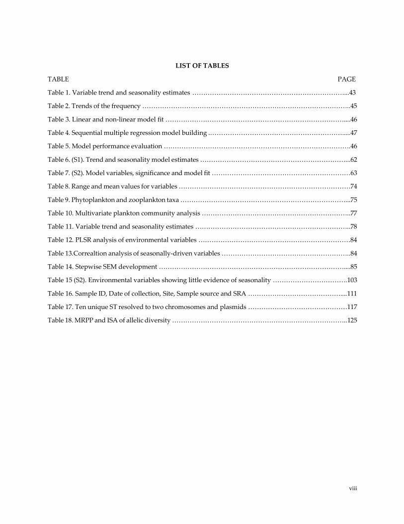
LIST OF TABLES

TABLE PAGE

Table 1. Variable trend and seasonality estimates ……………………………………………………………...43

Table 2. Trends of the frequency …………………………………………………………………………………..45

Table 3. Linear and non-linear model fit ………………………………………………………………………....46

Table 4. Sequential multiple regression model building .…………………………………………………….....47

Table 5. Model performance evaluation ………………………………………………………………………….46

Table 6. (S1). Trend and seasonality model estimates …………………………………………………………...62

Table 7. (S2). Model variables, significance and model fit ………………………………………………………63

Table 8. Range and mean values for variables ……………………………………………………………………74

Table 9. Phytoplankton and zooplankton taxa …………………………………………………………………...75

Table 10. Multivariate plankton community analysis …………………………………………………………..77

Table 11. Variable trend and seasonality estimates ……………………………………………………………..78

Table 12. PLSR analysis of environmental variables ……………………………………………………………84

Table 13.Correaltion analysis of seasonally-driven variables …………………………………………………..84

Table 14. Stepwise SEM development …………………………………………………………………………....85

Table 15 (S2). Environmental variables showing little evidence of seasonality …………………………….103

Table 16. Sample ID, Date of collection, Site, Sample source and SRA ……………………………………....111

Table 17. Ten unique ST resolved to two chromosomes and plasmids ………………………………………117

Table 18. MRPP and ISA of allelic diversity ……………………………………………………………………..125

ix

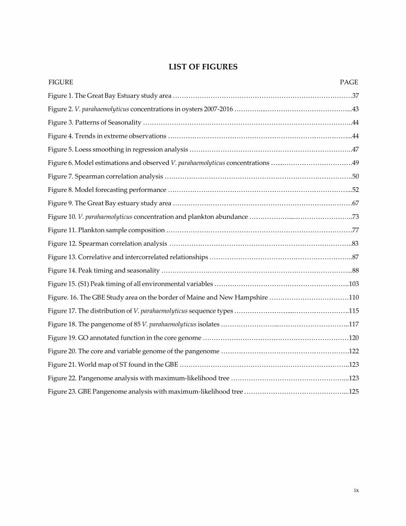
LIST OF FIGURES

FIGURE PAGE

Figure 1. The Great Bay Estuary study area ………………………………………………………………………37

Figure 2. V. parahaemolyticus concentrations in oysters 2007-2016 …………....………………………………...43

Figure 3. Patterns of Seasonality …………………………………………………………………………………..44

Figure 4. Trends in extreme observations ………………………………………………………………………...44

Figure 5. Loess smoothing in regression analysis ………………………………………………………………..47

Figure 6. Model estimations and observed V. parahaemolyticus concentrations …....………………………….49

Figure 7. Spearman correlation analysis ………………………………………………………………………….50

Figure 8. Model forecasting performance ………………………………………………………………………...52

Figure 9. The Great Bay estuary study area ………………………………………………………………………67

Figure 10. V. parahaemolyticus concentration and plankton abundance ………………....……………………..73

Figure 11. Plankton sample composition …………………………………………………………………………77

Figure 12. Spearman correlation analysis ………………………………………………………………………..83

Figure 13. Correlative and intercorrelated relationships ………………………………………………………..87

Figure 14. Peak timing and seasonality …………………………………………………………………………...88

Figure 15. (S1) Peak timing of all environmental variables …………………………………………………….103

Figure. 16. The GBE Study area on the border of Maine and New Hampshire ………………………………110

Figure 17. The distribution of V. parahaemolyticus sequence types ……………………....…………………….115

Figure 18. The pangenome of 85 V. parahaemolyticus isolates ……………………...…………………………..117

Figure 19. GO annotated function in the core genome …………………………………………………………120

Figure 20. The core and variable genome of the pangenome ………………………………………………….122

Figure 21. World map of ST found in the GBE …………………………………………………………………..123

Figure 22. Pangenome analysis with maximum-likelihood tree ……………………………………………...123

Figure 23. GBE Pangenome analysis with maximum-likelihood tree ………………………………………...125

x

ABSTRACT

FORECASTING VIBRIO PARAHAEMOLYTICUS IN A CHANGING CLIMATE

BY

Meghan A. Hartwick


The distribution, transmission and adaptation patterns of infectious diseases are

changing worldwide. Though there are many potential mechanisms that can transmit infectious

agents to new areas, the ability of pathogens to persist in new locations can be largely attributed

to changing climate conditions, especially in temperate regions. Vibrio parahaemolyticus, a

naturally occurring bacteria in most marine and estuarine systems, provides a model example

of these globally observed climate-related changes to disease dynamics that are occurring

locally in the Northeast, US. Like many Vibrio species, pathogenicity in human hosts is believed

to be limited to a subset of strains, whereas the overall population of various strains acts as a

part of the microbial community contributing to nutrient cycling and the food web. Until

recently, global V. parahaemolyticus disease incidence was sporadic and mainly limited to the

warm water regions of Asia, India and the Gulf of Mexico in the US. However, disease from

pathogenic V. parahaemolyticus has become endemic in cold and temperate-water regions,

including parts of Europe, Canada, and the Northwest and Northeast regions of the US that

were historically considered low risk for V. parahaemolyticus disease. The consumption of raw

or undercooked oysters is the most common route of V. parahaemolyticus infection, and the

xi

recent increase of illnesses in the Northeast has been simultaneous with a significant expansion

of the regional oyster fishery. The application of traditional environmental indicators such as

water temperature and salinity that were developed in warm water regions to mitigate and

manage disease risk have not been completely successful indicators for preventing the public

from becoming sick due exposure to pathogenic V. parahaemolyticus in this region. A

combination of statistical modeling and population genomic analysis was used to characterize

the ecology of V. parahaemolyticus in the Great Bay estuary (GBE) to better inform monitoring

and forecasting strategies to manage the impacts to public health and the shellfish industry of

these local outbreaks, since solutions from the warm and tropical regions may not be effective in

the temperate regions. Forecasting models were developed by combining ecological variables

with seasonality and trend analysis to analyze long-term surveillance data collected since 2007

(Chapter 1). High resolution investigation of the interactions between V. parahaemolyticus and

the plankton community was then used to characterize the environmental variables that

contribute to the development of optimal conditions for V. parahaemolyticus growth over the

course of a season (Chapter 2). Finally, genomic analysis of V. parahaemolyticus was conducted to

investigate how the environment influences population structure in the GBE and may

contribute to observed V. parahaemolyticus population dynamics (Chapter 3). Continued long-

term surveillance and forecasting tools are needed to address many of the currently unresolved

questions surrounding V. parahaemolyticus ecology that are important to better understand its

role as both a member of the environmental community and an agent of human disease. This

research provides an in-depth picture of the ecological drivers that underlie the interactions of

V. parahaemolyticus with its environment and contributes to the development of effective

xii

forecasting tools for public health and shellfish management under current and future climate

scenarios.

1

INTRODUCTION

In recent years, disease from pathogenic Vibrio parahaemolyticus has emerged in cold and

temperate-water regions that were historically considered low risk for V. parahaemolyticus

disease outbreaks (Makino et al., 2003; Newton et al., 2013; CDC, 2013; Xu et al., 2015). The

expansion of pathogenic strains into these regions, that were believed to be unlikely to support

disease causing strains, has become a focal point of study for both public health and the seafood

industry to identify the conditions that led to this new pattern of V. parahaemolyticus disease and

prevent it from occurring in the future (Baker-Austin, Trinanes, Gonzalez-Escalona, &

Martinez-Urtaza, 2017; Semenza et al., 2017; Vezzulli et al., 2013; 2009; Deter et al., 2010,

McLaughlin et al., 2005).

Vibrio parahaemolyticus disease is an ongoing public health problem worldwide. Since V.

parahaemolyticus was first identified in 1953 (Fujino et al., 1953) over fifty years of spatially and

temporally intense ecological, mechanistic and genetic studies around the globe have

demonstrated that V. parahaemolyticus is a highly adaptable organism that utilizes a complex

array of mechanisms to persist in most biotic niches and abiotic conditions as a ubiquitous

component of marine and estuarine ecosystems (Hartwick et al., 2019; Kaneko & Colwell, 1973;

Lovell, 2017; Martinez-Urtaza et al., 2012; Turner et al., 2014; Urquhart et al., 2014.; Vezzulli et

al., 2009; Jones and Summer-Brason 1998, DePaola et al., 1990). This adaptability is likely one of

the main features that enables V. parahaemolyticus to simultaneously act as both a component of

environmental ecosystems and a human pathogen (Espejo, García, & Plaza, 2017; Johnson, 2013;

2

Turner et al., 2016). Therefore, predicting V. parahaemolyticus disease risk requires a thorough

characterization of its ecology.

This review is a synthesis of the ecological, virulence, and population genomic traits of

Vibrio parahaemolyticus to address the current challenges to the development of forecasting

models for V. parahaemolyticus disease in temperate water regions. The goal of this work is to

highlight potential directions that could improve methods and produce new knowledge to

address the ecological complexity of V. parahaemolyticus dynamics. A more in-depth

understanding of these adaptation patterns will provide the foundation for the development of

effective forecasting methods for V. parahaemolyticus risk in the temperate regions that now

experience frequent and reoccurring V. parahaemolyticus disease outbreaks.

Ecosystem traits

The ecology of Vibrio parahaemolyticus has been the focus of many studies that applied a

combination of long-term monitoring and intensive short-term observation across the globe.

The first comprehensive report by Kaneko and Colwell (1973) detailed the complex seasonal

dynamics that contributed to the emergence and persistence of V. parahaemolyticus in the

estuarine environment of the Chesapeake Bay. It highlighted that V. parahaemolyticus was

present in many environmental niches and that a wide range of abiotic and biotic factors are

associated with its presence and accumulation in these niches, including water temperature,

salinity, and plankton. Since then, the number of potentially important environmental factors

have broadened considerably (Takemura, Chien, & Polz, 2014).

Abiotic

3

Bulk water abiotic features play a large part in the growth rate of Vibrio parahaemolyticus

in coastal aquatic ecosystems. Temperature is recognized as the most important abiotic factor to

modulate V. parahaemolyticus growth and concentration (Takemura, Chien & Polz, 2014). The

lower threshold for growth is around 15°C, though it has been recovered from temperate and

cold-water regions at 4°C (Hartwick et al., 2019; Oberbeckmann et al., 2011). The ideal range in

pure cultures is between 25-35°C.

V. parahaemolyticus is halophilic and is recovered from a wide range of salinities in

estuarine, marine, and brackish water, indicating that its tolerance and requirements for salinity

are broad and this abiotic parameter may not be a restrictive growth parameter (Lopez-

Hernandez et al., 2015; Paranjpye et al., 2015; Young et al., 2015; Oberbeckman et al., 2012,

DePaola et al., 1990). Similarly, V. parahaemolyticus is also classified as a facultative anaerobe,

indicating that dissolved oxygen (DO), which modulates inversely with water temperature, is

not a restrictive growth parameter (Blackwell & Oliver, 2008; Caburlotto et al., 2010). However,

in vivo studies show that ideal conditions for V. parahaemolyticus are a neutral pH (Wong et al.,

2004). Mildly basic conditions are well tolerated, however conditions considered mildly acidic

are inhibitive to growth and persistence (Wong et al., 2015). The measured ranges of

environmental variables that relate to V. parahaemolyticus growth vary widely between studies

and locations. This stems from site-specific differences in V. parahaemolyticus ecology. However,

study design and analytic methods have also been cited as key points contributing to

differences in the reported influence of these abiotic parameters (Takemura et al., 2014, Froelich

and Noble, 2016).

4

Biotic

Studies on the biotic aspects of coastal ecosystems frequently focus on interactions

between Vibrio parahaemolyticus and the plankton community. V. parahaemolyticus-plankton

dynamics, first reported by Kaneko and Colwell (1975), determined that this interaction

provided a key source of nutrients for growth and persistence, while also providing protection

from predation and enhancing nutrient acquisition. Chitinous diatoms and dinoflagellates, such

as Skeletonemia spp. and Chaetocerous spp., as well as copepods in the zooplankton community

are significantly associated with the presence and concentration of V. parahaemolyticus in the

environment (Gilbert et al., 2012). Further, chitin promotes horizontal gene transfer through

chitin-induced competence, suggesting that the plankton community may play an important

role in the evolutionary dynamics as well (Meibom et al., 2005; Pruzzo, Vezzulli, & Colwell,

2008).

Direct investigation of Vibrio parahaemolyticus-plankton dynamics can sometimes prove

to be inhibitive due to the additional logistics required to effectively characterize plankton

species and concentrations. As such, proxies have been applied to more effectively characterize

these interactions such as chlorophyll-a, organic and inorganic nitrogen, phosphate, carbon, as

well as silicate, (e.g. Paranjpye et al., 2015, Turner et al., 2013). Chlorophyll-a is frequently found

to be a positively correlated parameter, whereas the statistical relationship between nutrients

and V. parahaemolyticus are generally much more variable (Takemura, Chien and Polz, 2014,

Oberbeckman et al., 2011, Blackwell and Oliver, 2008). The variable statistical relationship of

nutrients to V. parahaemolyticus dynamics is attributed to the indirect role of nutrients in the

vibrio-plankton dynamics. The importance of nutrients should not be undervalued in

5

characterizing the Vibrio-plankton dynamics interactions, however it is unlikely that nutrient

measurements will be helpful for prediction in forecasting methods (Gude, 1985).

Different sample sources, referred to as ecosystem matrices, including sediment, water

and shellfish are also a frequent interest in studies on the biotic ecology of Vibrio

parahaemolyticus (Nilsson et al., 2019; Di et al., 2016; Deter et al., 2010). Sediment provides

nutrients as well as insulation from predators for V. parahaemolyticus, especially during fall,

winter and spring in cold and temperate water regions (Alipour et al., 2014; Vezulli et al., 2009;

Kaneko and Colwell, 1973). The water column is also considered an important detection point

for V. parahaemolyticus, though it is frequently the organic enriched fractions of the water

column, including marine snow, detritus and suspended sediment that are the point of interest

for these studies (Williams et al., 2014; Froelich et al., 2013). This is based on findings that

suggest that V. parahaemolyticus prefers an attachment vs free living lifestyle and therefore is

more likely to associated with these organic fractions (Johnson et al., 2012; Lovell, 2017; Parveen

et al., 2008). Under certain conditions (i.e. phytoplankton blooms), V. parahaemolyticus can thrive

in a free-living lifestyle by subsisting mainly off of polysaccharide exudate from the

surrounding environment (Gilbert et al., 2012; Venkataswaran, 1990). This finding highlights

the importance of algal blooms as a nutrient source for V. parahaemolyticus, but also provides

new insight into strategies employed by free-living V. parahaemolyticus for persistence in the

environment.

Whether shellfish are a preferred environment for Vibrio parahaemolyticus remains

unclear, however because of their commercial importance, the shellfish-V. parahaemolyticus

relationship is the most frequently studied interaction. The dynamics of V. parahaemolyticus have

6

been studied in many shellfish species including hard shell clams, razor clams and mussels

(Lovell, 2017). However, the commercially important oyster species Crassostrea virginica and C.

gigas have been the focus of the majority of V. parahaemolyticus studies (Zimmerman et al., 2007;

DePaola et al. 1990, 2003). Filter feeding of suspended material is the most likely route by which

V. parahaemolyticus becomes concentrated in shellfish (i.e. Froelich et al., 2013). Kaneko and

Colwell (1973) first described how this filter feeding likely leads to the annual emergence of V.

parahaemolyticus in the Chesapeake Bay as a seasonal cycle between sediment, water, plankton,

and shellfish.

In addition to the major biotic relationships that have been described for Vibrio

parahaemolyticus, incidental associations and disease in macroalgae, fish and marine mega fauna

have also been reported, including outbreaks of V. parahaemolyticus-caused mortality in shrimp,

ornamental fish and corals (Vezzulli et al. 2012), as well as isolated cases of V. parahaemolyticus

associated abscesses and lesions in dolphins, sea otters, harbor seals, finfish, and crustaceans

(Lovell, 2017; Hughes et al., 2013; Martinez-Urtaza et al., 2010).

Ecology in summary

From a public health perspective, the complex combination of conditions that relate to

the growth and persistence of Vibrio parahaemolyticus in the environment necessitates that most

preventative measures rely on the use of broad environmental indicators to prevent the public

from becoming sick due exposure to V. parahaemolyticus. Water temperature, salinity, and V.

parahaemolyticus concentration are among the most commonly applied criteria employed in risk

assessments (DePaola et al., 2003; FDA, 2005; Lovell, 2017). However, many studies have

observed that V. parahaemolyticus disease outbreaks from the consumption of raw or

7

undercooked seafood do not always coincide with high concentrations of V. parahaemolyticus in

the environment, nor the ecosystem conditions that are thought to promote its abundance

(Paranjpye et al., 2015). Ideally, preventative methods should be coupled with monitoring for

conditions that enrich for potential human-specific pathogens. Such an approach is currently

limited, in part, by the need to better identify the causative virulence trait in humans that would

then allow determination of what conditions in the environment may promote the abundance of

this trait. The penultimate virulence mechanism has not yet been confirmed though many traits

associated with virulence in humans have been reported and characterized that can provide

insight into the mechanisms that may contribute to V. parahaemolyticus disease in humans

(Ceccarelli et al., 2013; Whistler et al., 2015; Xu et al., 2017, 2015).

Virulence associated traits

Vibrio parahaemolyticus disease can be caused by multiple different sequence types and

recognized virulence associated traits are equally absent or present in isolates recovered from

clinical patients. Given these conditions, it has been suggested that human infection and disease

from V. parahaemolyticus may therefore be the result of trait(s) that aid in environmental

persistence rather than evolved human-specific mechanism(s) like those observed in obligate or

opportunistic human pathogens. For this reason, there is a growing recognition that V.

parahaemolyticus may be an accidental human pathogen whose human pathogenicity is an

exaptive trait(s) that aid in persistence in the marine and estuarine environment (Turner et al.,

2017; Johnson et al., 2013).

8

Virulence factors in bacteria can include traits that aid in colonization, attachment,

immune evasion, and competition and nutrient acquisition via toxins, all of which have been

identified in Vibrio parahaemolyticus in the form of flagella, capsule production, hemolysins,

enterotoxins, cytotoxins, proteases, siderophores and hemagglutinin (Johnson, 2013). The most

recognized and studied of these traits are the hemolysins tdh and trh, though genes for the Type

III Secretion Systems (T3SS) are increasingly being recognized for their potential contribution to

causing disease. The virulence-associated traits tend to co-occur on pathogenicity islands (VPaI)

that have are dynamically shared between strains via horizontal gene transfer and

recombination. In conjunction with the inconsistent detection of tdh, trh and T3SS in clinical

cases (Lovell, 2017; Nishibuchi et al., 1992; Shinoda & Miyoshi, 2006), the dynamic exchange of

VPaIs and the ubiquitous presence of virulence associated traits in ‘environmental’ and ‘clinical’

strains alike have been a major hurdle to developing targeted preventative public health

measures (Ceccarrelli et al., 2013).

Hemolysins

Pore forming toxins such as hemolysins are the mechanism of pathogenicity employed

by many bacterial species including Escherichia coli, Mycobacterium tuberculosis and

Staphylococcus aureus and act by disrupting host cell membranes to directly kill target cells, to

evade immune detection, and/or to release nutrients (Los et al., 2013). Hemolysin gene

products of Vibrios have been shown to lyse host erythrocytes and may be used to access the

nutrients bound within host cells. The thermolabile hemolysin gene (tlh), thermostable direct

hemolysin (tdh) and the tdh-related hemolysin (trh) genes are the most commonly used potential

virulence traits in Vibrio parahaemolyticus (Xu et al., 2017; Lovell, 2017; Ceccarelli et al., 2013;

9

Johnson et al., 2013). They are generally used in a multiplex polymerase chain reaction to

identify V. parahaemolyticus and help to differentiate potential pathogenic strains. The first PCR

primers developed for detection of tlh, tdh, and trh were described by Bej et al. (1999) who used

them in multiplex PCR to detect all three genes simultaneously (Lovell, 2017).

The tlh gene encodes a thermolabile hemolysin. The specific function of this gene in

human infection is unknown though the tlh gene is widely considered to be a species-specific

marker for Vibrio parahaemolyticus (Klein et al., 2014; Johnson, 2013). The tdh and trh genes, are

approximately 67% identical and are predicted to function in similar manners (Johnson et al.,

2013). Products of tdh, an amyloid toxin and trh, which is believed to act by activating Cl-

channels (Ceccarelli et al., 2013), embed in and disrupt host cell membranes, acting as porins.

This can be detected in vitro by lysis of erythrocytes, as demonstrated by β-hemolysis (the

Kanagawa phenomenon) on saline blood agar (Wagatsuma Agar)(Klein et al., 2014; Lovell,

2017). Both tdh and trh sequences can vary widely, they are separated on the two chromosomes

and are typically harbored on islands (Xu et al., 2017) in many V. parahaemolyticus strains

(Lovell, 2017).

In 1996, the surveillance testing in Kolkata, India, determined that a novel serotype,

O3:K6, accounted for 50–80% of Vibrio parahaemolyticus gastroenteritis infections were tdh+/trh-

(Ceccarelli., et al., 2013). Whereas almost all V. parahaemolyticus strains isolated from clinical

samples possess beta-hemolytic activity attributed to these two genes (Ceccarelli et al., 2013),

about 10% of clinical strains do not contain tdh and/or trh (Xu et al., 2015; Raghunath, 2014).

More in-depth environmental studies have now shown that the detection of tdh and trh in the

environment can vary from to 1–2% of total strains to upwards 48-52% of isolates. Whereas tdh

10

and trh are still used to identify potential virulent strains, the prevalence of these genes in

environmental V. parahaemolyticus strains has led many to suspect that their role is not solely to

contribute to human disease (Lovell, 2017).

Secretion systems

The range of hemolysin profiles in Vibrio parahaemolyticus strains recovered from

patients with clinical V. parahaemolyticus disease prompted many researchers to look beyond

tdh, trh and tlh to determine additional factors that may underlie virulence in V.

parahaemolyticus. Secretion systems, which are used by most bacterial species for routine

functionality can be essential to pathogenesis for Salmonella, Shigella and Yersinia (Hapfelmeier

et al., 2005). Six secretion systems (T1SS-T6SS) have been described in gram negative bacteria, of

which two (T3SS and T6SS) are of central interest as potential sources of virulence in V.

parahaemolyticus because of their recognized role in promoting toxicity, immune evasion and

cell adherence (i.e. Zhang & Orth, 2013).

T3SS use a ‘needle-like apparatus’ to insert a range of effector proteins that can cause

cytotoxicity or enterotoxicity (Ceccarelli et al., 2013) or inhibit immune systems or forcing the

induction of host cell apoptosis (Blondel et al., 2016; Zhang & Orth, 2013). They are also

important for attachment and colonization in intestinal systems and in extra-intestinal systems.

T3SS1, identified by Makino et al., (2003) is located on chromosome one and is well conserved

and widespread in both clinical and environmental strains of V. parahaemolyticus (Ceccarelli et

al., 2013). Identified as vscC1, the T3SS1 gene cluster is composed of 42 genes (Lovell, 2017).

Collectively, T3SS1 effectors are reported to evade the host immune response and to cause

11

cytotoxic damage in the host cells to acquire nutrients from non-erythrocyte host cells Johnson

(2013).

T3SS2 is found on chromosome two, identified by vscC2 (Makino et al. 2003) and there

are two T3SS2 variants (Johnson, 2013; Lovell, 2017). T3SS2 is believed to be necessary to deliver

toxin proteins into host cells and plays a role colonization, immune avoidance, and acquisition

of nutrients. Unlike T3SS1, it is not present in all Vibrio parahaemolyticus strains. Because of its

variability and dual role in toxicity and immune avoidance, the gene for an outer membrane

protein (vscC) has also been used as a marker for virulent V. parahaemolyticus (Klein et al., 2014;

Park et al., 2004). Recent findings demonstrated that, along with its six effectors, T3SS2- α

allows V. parahaemolyticus to invade, survive, and replicate in non-phagocytic host cells (Zhang

& Orth, 2013).

Two T6SS have also been identified in Vibrio parahaemolyticus and are distributed

between the two chromosomes (Boyd et al., 2008). T6SS were only recently identified by

(Pukatzki et al., 2006) in V. cholerae, where it is believed to contribute to mediate extracellular

export of virulence factors and injection into eukaryotic host cells (Boyd et al., 2008). Its role in

V. parahaemolyticus has not yet been fully determined (Johnson, 2013). Preliminary data suggest

that it is involved in adhesion to host cells (Yu et al., 2012). Since T6SS2 and T3SS2 co-exist, it

was proposed that the two systems might cooperate during infection. T6SS2 plays its role in

adhesion, the first step of infection, and T3SS2 exports effectors by inducing entero-cytotoxicity

(Ceccarelli et al., 2013; Yu et al., 2012; Park et al., 2004)

Interactions between virulence factors have been suggested not only within secretion

systems but also between hemolysins and secretion systems. Early studies, which reported a

12

correlation between the presence of T3SS2α and tdh and separately T3SS2β with trh, led to the

hypothesis that the former was a requirement for strains to be Kanagawa positive (Baker-Austin

et al., 2010). Whereas recent findings appear to disprove this correlation based on the detection

of a wide range of combinations of tdh, trh and T3SS2s and Kanagawa phenotype within strains

(Jones et al., 2012; Paranjpye et al., 2012), it has been determined that hemolysins and secretion

systems tend to co-occur in regions of the genome referred to as pathogenicity islands (Lovell,

2017; Xu et al., 2017; Klein et al. 2014; Ceccarelli et al., 2013)

Vibrio pathogenicity islands

Pathogenicity islands are groups of genes with virulence-associated traits that can be

transferred and acquired holistically by horizontal gene transfer facilitated by phage, plasmid or

induced competence. They carry genes that can provide some benefit to V. parahaemolyticus for

persistence, usually to enhance competition or nutrient acquisition (Johnson, 2013; Ceccarelli et

al., 2013) Nine pathogenicity islands have been defined in RIMD (VPaI-1 to VPaI-9), and these

can be located on either chromosome and are differentially distributed between strains (Boyd et

al., 2008; Hurley et al., 2006). Homologous VPaIs have been identified in other strains. Initially,

they were considered a useful marker to identify specific pathogenic strain types, particularly

those that were associated with pandemic disease. However, it has been difficult to establish a

pattern between the presence of a VPaI and strains that could be classified as a pandemic,

environmental or clinically associated. Strains of sequence-types or serotypes that are associated

with disease do not always contain the VPaI to which they are generally attributed, and non-

pathogenic non-pandemic strains have been found to contain the VPaIs typically used as

markers for pathogenic strains (Makino et al., 2003).

13

Despite the rapidity of exchange that appears to occur with VPaIs between strains, Xu et

al., (2017) recently demonstrated that they can be invaluable to characterizing early events that

lead to the differentiation of environmental strains to become potential human pathogens.

Further, the variable presence and content of VPaIs provides enormously valuable insight into

the amount and frequency of exchange of genetic materials that occurs within the V.

parahaemolyticus genome in the environment. The size and GC content of these VPaIs suggests

that they are most frequently acquired via horizontal gene transfer (Boyd et al., 2008; Hurley et

al., 2006). In addition, the genetic content of these islands varies between genetic material that

is shared between V. parahaemolyticus strains and material that may have been acquired from

other species, for example: homologs of the Escherichia coli cytotoxic necrotizing factor (CNF)

and Pseudomonas exoenzyme T identified in VPaI-7 (Ceccarelli et al., 2013; Makino et al., 2003)

Pathogenicity islands show potential utility as a marker that can be used to identify and

differentiate strains with pathogenic potential as well as a tool to observe the dynamics of

genetic exchange via constant recombination within V. parahaemolyticus. However, in addition

to hemolysins and T3SS and T6SS, V. parahaemolyticus is also equipped with an additional suite

of genetic traits that are considered virulence-associated traits. These include quorum sensing,

biofilm formation, proteases and chitinases, and siderophores (Johnson, 2013).

Quorum sensing and biofilms

Quorum sensing is used by many bacterial species to regulate cell density through

chemical signaling to control gene expression (Johnson, 2013). This process of signaling has

been shown to regulate hundreds of genes involved in virulence factor production and growth.

AphA and OpaR are the two master regulators of quorum sensing in Vibrio parahaemolyticus (Sun

14

et al., 2012; Zhang et al., 2012), where AphA is expressed at low cell density and OpaR is

expressed at high cell density (Zhang et al., 2017). Expression of T3SS secretion machinery genes

in V. parahaemolyticus (T3SS1) are dependent upon a functional quorum sensing system; at high

cell densities, quorum sensing decreased T3SS activity in both species (Johnson, 2013). Recent

work suggests that quorum sensing plays a role in the self-limiting dynamics of gastro-

intestinal infection by V. parahaemolyticus and may have an ecological advantage for resource

competition.

In addition to controlling the production of metabolites, quorum sensing also regulates

the production of biofilms (Davey & O’toole, 2000; Jayaraman & Wood, 2008). Biofilm formation

is a complex process that involves the production of a polysaccharide matrix that acts as a

mechanism of attachment and protection from external threats from the host and other bacterial

species. It has been shown to be essential for colonization of a host and in vitro studies have

demonstrated that strains that are deficient in biofilm production factors are less successful in

causing infection and disease (Johnson, 2013).

Chitinases and proteases

Chitin is one of the most abundant molecules in the marine and estuarine environment

and is used by Vibrio parahaemolyticus as a source of nutrients. V. parahaemolyticus produces

chitinases, a class of enzymes that can breakdown chitin into accessible carbon monomers.

GbpA, one of the more well characterized genes involved in this process has also been shown in

V. cholerae to facilitate attachment to surfaces as well including chitinaceous plankton and

intestinal cell wells (Johnson, 2013). In vitro studies show that mutants lacking GbpA had

lowered resilience to unfavorable environmental conditions including various temperatures

15

and salinities (Johnson, 2013). The study of the function of GbpA in V. parahaemolyticus is

ongoing (Tiruvayipati & Bhassu, 2016; Tiruvayipati et al., 2013) but preliminary outcomes from

in vivo observation suggest its serves a similar role in attachment and chitin utilization.

Proteases are another class of enzymes used by Vibrio parahaemolyticus to access

nutrients. Target-specific proteases convert proteins into usable forms for V. parahaemolyticus.

Proteases are key toxicity factors in many pathogenic bacterial species for example Bacillus

anthracis, the causative agent of anthrax and are recognized to play pathogenic roles following

the initial infection (Shimodo and Myoshi, 2006). Two metalloproteases and one serine protease

has been identified in V. parahaemolyticus. The serine protease, encoded by proA has been shown

to cause erythrocyte lysis, cell toxicity and death in mice and cell culture (Johnson, 2013). The

metalloproteases in V. parahaemolyticus are encoded by PrtV and VppC. Whereas

metalloproteases have been shown to be key components of both botulinum and tetanus toxin,

their potential role in V. parahaemolyticus has not been well characterized (Shimodo and Myoshi,

2006).

Virulence associated traits in summary

A thorough assessment of the virulence-associated traits found in Vibrio parahaemolyticus

provides insight into the potential mechanisms it employs for persistence in the environment

and the human host. The virulence-associated traits identified in V. parahaemolyticus can be

considered as two components of the disease process. Traits such as hemolysins (tdh and trh),

toxins from secretion systems and proteases produce the diseased state, whereas traits involved

in motility (flagella), immune evasion (capsule production) and adhesion (biofilm formation)

16

enable V. parahaemolyticus to overcome host defenses or competition to establish the infection

(Lee et al. 2015; Ceccarelli et al. 2013; Shinoda and Miyoshi, 2006).

The lack of a definitive human disease-causing trait that all pathogens contain is clearly

one of the most important challenges to overcome in order to develop targeted methods for

forecasting disease risk. In its absence, virulence associated markers or traits such as tdh, trh,

and more recently T3SS and VPaIs have been used as markers to differentiate potential

pathogens from total Vibrio parahaemolyticus to provide some differentiation of risk between

inert and potential pathogenic strains, but these approaches have noted limitations. Successful

forecasting methods for V. cholerae have focused on O1 and O139, and likewise monitoring for

V. parahaemolyticus disease risk have focused on detection of genes in known pathogenic

serotypes or sequence types such as ST3 and ST36, which are known to have pandemic

distribution. However, because of the rapidity of genetic exchange between strains, this has

been found to have limitations as well. In part because the pandemic strain has evolved since its

emergence in 1998 and isolates have been found to be missing key virulence associated traits.

Further, environmental V. parahaemolyticus strains have been isolated with pathogenicity islands

identified to be key to human virulence including VPaI-7 andVPaI-2 (Ceccarelli et al., 2013;

Gennari et al., 2012). Given this, effective epidemiological reconstruction and investigation of

the mechanisms of pathogen emergence will require accounting for the many potential sources

of underlying diversity within populations by accounting for the evolutionary dynamics acting

on V. parahaemolyticus at both the genome and population level. These particular features make

epidemiological phylogenetic analysis and risk forecasting of V. parahaemolyticus disease

especially challenging.

17

Population genomics and genetics

Rapid development of low cost, high throughput sequencing in recent years has

provided tremendous insight into the evolutionary and population dynamics of Vibrio

parahaemolyticus that contribute to the genetic flexibility that is a characteristic trait of V.

parahaemolyticus. The complete genome of pandemic strain RIMD, published in 2003 (Makino et

al. 2003), provided the first real opportunity to assess the basic structure and functionality of V.

parahaemolyticus in its entirety. The first complete representative genome of V. parahaemolyticus

was a pandemic O3:K6 strain, now commonly referred to as RIMD (2210633) that was recovered

from an individual with food poisoning in 1996. RIMD is composed of two circular

chromosomes, containing approximately 4832 coding sequences, with a GC bias of 45.4% and

approximately 40% of coding sequences were annotated as hypothetical proteins. Chromosome

one was found to be larger, containing 3080 coding sequences, many of which were involved in

basic cell functions such as growth and viability, whereas chromosome two consisted of

approximately 1752 coding sequences and had more genes related to metabolism and

environmental regulation.

Since it was first sequenced, over 800 Vibrio parahaemolyticus genome assemblies have

been made available through NCBI and >1800 ST profiles are included in the V. parahaemolyticus

multi locus sequence type (pubMLST) database. This helps to illustrate why forecasting disease

risk has proven such a challenge by demonstrating the amount of diversity that evolves and is

maintained in V. parahaemolyticus populations. The variable presence and mobility of virulence-

associated traits can be attributed to the major forces of mutation, horizontal gene transfer and

recombination shaping the V. parahaemolyticus genome. Whereas both variable mutation rates

18

across the genome and horizontal gene transfer and have been shown to play a role in V.

parahaemolyticus evolution (Tamames, Sánchez, Nikel, & Pedrós-Alió, 2016), many believe that

HGT and recombination is the predominant force shaping the V. parahaemolyticus genome

(Ceccarelli et al., 2013; Johnson, 2013; Martinez-Urtaza et al., 2017). Historically, phylogenetic

assessment has been the most widely used epidemiological tool to trace the evolutionary

background or trajectory of the emergence of virulence within a population. However, the

ability of V. parahaemolyticus to undergo recombination, even in conserved regions believed to

be limited to vertical acquisition, potentially masks many of the patterns typically used to assess

the development and succession of virulent lineages within largely non-pathogenic

populations. Given this, effective epidemiological reconstruction and investigation of the

mechanisms of pathogen evolution will require accounting for the many potential sources of

underlying diversity within populations.

Recombination and mutation

The structure and content of the Vibrio parahaemolyticus genome appears to be largely

facilitated by variable mutation rates combined with gene gain and loss. The overall genomic

content consists mostly of coding sequences (identified and hypothetical) with very little

intragenic or pseudogenic content (~5,000 orf and 5mb). This is consistent with what is observed

in most free-living bacterial species where gene number is observed to be a direct linear

relationship to genome size.

The process that results in this densely packed genome is known as genome reduction.

A number of factors can contribute to this, each providing insight into the evolutionary forces

shaping the genome. Metabolic efficiency has been suggested as one these selective

19

mechanisms. Vibrio parahaemolyticus, which has 11 copies of rRNA operons, higher than in many

other prokaryotes (Makino et al., 2003), can undergo replication in ideal environmental

conditions every 8 minutes. The metabolic cost of maintaining non-essential genetic material

could be a prohibitive cost in resource limited environments (Abu Kwaik & Bumann, 2013,

2015). The genome streamlining hypothesis, which has mixed support from experimental and

comparative studies, proposes that material that is not essential represents a negative metabolic

cost and therefore selection deletes superfluous content from the genome via mutation

accumulation and deletion (Bobay & Ochman, 2017; Weinert & Welch, 2017). Therefore, genome

reduction would make the organism more fit for rapid replication in nutrient-limited

environments. In contrast, genome reduction in host-associated pathogens occurs through

gradual loss of function in regions that are no longer needed by the organisms and are

recognizable by the presence of extra genetic material including pseudogenes (Bobay and

Ochman, 2017).

Genome reduction has also been proposed to indicate environmental adaptation and

evolution within the individual towards niche specialization. Martinez-Urtaza et al., (2017),

found a trend toward gene number reduction in ST36, where larger genomes and higher gene

numbers were observed in strains from older subpopulations than in modern U.S. strains,

suggesting that the gene number reduction could be associated with a more specialized lifestyle

as a result of niche adaptation in the US. Thus, genome reduction may have multiple

evolutionary benefits to control the metabolic cost to Vibrio parahaemolyticus and facilitate

adaptation when exposed to new selective pressures (Bobay & Ochman, 2017).

20

The major driver of evolution and adaptation in Vibrio parahaemolyticus, however, is

attributed to the acquisition of novel genetic material through homologous and non-

homologous recombination and mutation (Bobay and Ochman, 2017, Ceccarelli et al., 2013;

Johnson, 2013). Horizontal gene transfer through recombination, phage or plasmid enables

bacteria to adapt to new environmental niches, trait sharing such as antibiotic resistance or

pathogenicity islands (Metzger & Blokesch, 2014). Homologous recombination also provides the

resources for niche adaptation and diversification. The current genetic divergence within ST36

clonal populations has been attributed to recombination (Martinez-Urtuza et al., 2017, Xu et al.,

2017). Whereas the most recognized mechanism for rapid niche adaptation in V.

parahaemolyticus is homologous recombination and horizontal gene transfer, Johnson et al.,

(2013) suggested that elevated mutation rates may also facilitate niche adaptation.

The diversity among clinical and environmental Vibrio parahaemolyticus populations has

frequently been examined using multilocus sequence analysis and these studies reveal highly

diverse populations. Many hypothesize that organizing the diversity of V. parahaemolyticus to

environmentally relevant structures within these populations could be key to understanding

and forecasting V. parahaemolyticus dynamics and disease risk (Fraser et al., 2009). However,

assigning this diversity to ecological drivers has proven to be complex. In one study, diversity

was associated with geography (Cui et al., 2015), however most traditional phylogenetic

methods such as Multi-Locus Sequence Typing (MLST) have not produced isolate clustering

that relates to geographic, environmental, or pathogenicity factors (Ellis et al., 2012; Thompson

et al., 2004; Urmersbach et al., 2014).

21

Ecotypes

The diversity within and between Vibrio parahaemolyticus populations can be driven by

the demands of the environment they inhabit. This idea of “niche sequestering” was observed

and reported by Johnson et al., (2012) in strains from the Gulf of Mexico and Shapiro and Polz

(2014) where V. parahaemolyticus strains from similar environmental niches were more similar in

genetic content and allelic diversity than they were to strains that were isolated from different

environmental conditions. These observations are part of the basis for proposing that V.

parahaemolyticus populations may be structured into ecological species, or ecotypes. Ecotypes

can be understood as sub-populations that interact with other strains within their niche but

have limited exposure to V. parahaemolyticus that do not interact within the same microhabitats

in the environment. Because of this genetic isolation, strains that inhabit similar niches will have

more similar allelic diversity and accessary genomes (Friedman, Alm, & Shapiro, 2013).

Ecotypes provide an appealing mechanistic concept to connect environmental

conditions to population dynamics, and the water column provides a diverse range of resources

and nutrient patchiness that is an ideal environment for the development of micro-niche

specialization (Cohan, 2002; Cordero & Polz, 2014; Hunt et al., 2008; Shapiro & Polz, 2014).

Though Keymer et al., (2007) and Hunt et al., (2008) have identified potential Vibrio ecotypes by

allelic variation or variable genome content, ecotypes have not been frequently identified within

environmental populations (Bendall et al., 2016).

2nd Chromosome adaptation

Vibrio parahaemolyticus may also more rapidly undergo environmental adaptation

through its smaller, second chromosome. The second chromosome in Vibrio is hypothesized to

22

have arisen from the acquisition of a plasmid that provided a fitness benefit and was

maintained and evolved to be essential to V. parahaemolyticus function. It has been noted

frequently that the second chromosome tends to be enriched in genetic functions related to

environmental persistence, leading to the theory that the second chromosome retains its role as

a resource for the integration of novel material for environmental adaptation and persistence

(Ellis et al., 2012; Makino et al., 2003; Morrow & Cooper, 2012). In other organisms, this concept

is supported by higher substitution rates, greater dispensability, and lower codon usage bias for

genes on secondary chromosomes (Cooper et al., 2010; Holden et al., 2004). Similarly, GC bias

and a higher proportion of genes unique to each isolate (chromosome one: 56.8%, chromosome

two: 29.5%) have been reported in V. parahaemolyticus (Ceccarelli et al., 2013, Makino et al.,

2003).

Population dynamics in summary

The complexity of predicting Vibrio parahaemolyticus dynamics can be better understood

through the scope of the mechanisms that drive its genomic and genetic diversity. SNP analysis

of regions of interest, most frequently within housekeeping genes, has been used extensively to

establish genetic relationships between strains and potentially trace the emergence of

pathogenic lineages. However, horizontal gene transfer through homologous and non-

homologous recombination is also a major driving force of V. parahaemolyticus evolution that

may provide more information about the ecological drivers that are shaping the population

(Metzger and Blokesch, 2014). Therefore, the population genetics and genomics are shaped by

both lineage and the environment (Tamames et al., 2016). The relationship between gene

23

content and the environment remains to be clarified, however the mechanisms potentially

contributing to ecotype differentiation and niche specific adaptation through variable genome

content are an important potential direction to better determining the basis for how

environmental adaptation shapes V. parahaemolyticus dynamics.

Forecasting disease risk

Since the link between Vibrio disease dynamics and the environment was first

recognized, there has been a huge effort worldwide to characterize the ecology of Vibrio

parahaemolyticus to understand where and when human-health risks will occur (Nilsson et al.,

2019; Vezzulli et al., 2009). Takemura, Chien and Polz (2014) provided an excellent summary of

the differing and often conflicting outcomes of the reported correlative relationships between V.

parahaemolyticus and the more common environmental variables that are assessed including

water temperature, salinity, dissolved oxygen, turbidity and chlorophyll-a. This ecological

complexity could arise from region-specific and even site-specific environmental differences as

well as differences in local Vibrio parahaemolyticus population genetics and genomics (Froelich

and Noble, 2016; Shapiro and Polz, 2014). These are certainly contributing factors, however

there are also widely ranging differences in analytic, temporal and spatial study designs that

may also be contributing to this observed complexity. For example, though multiple regression

and correlation analysis are the most frequently applied analytic methods, season-specific

segmentation, lagged relationships exceeding one month, polynomial transformations and

descriptive splines between ecological and temporal relationships (Nilsson et al., 2019; Davis et

al., 2019; 2017; Paranjpye et al., 2015; Froelich et al., 2012) are also used and could influence the

importance of observed relationship of environmental variables. The majority of studies are also

24

often short-term observations between one summer season or less than two years, and

frequently group together multiple monitoring stations that may have widely ranging site

characteristics. Though ecological inference may be made from these kinds of studies, they are

limited in their ability to provide standardized comparisons between regions or to develop

transferable forecasting models.

Other important considerations within these outcomes of Vibrio parahaemolyticus

ecological studies are geographic distribution, transmission and adaptation patterns. V.

parahaemolyticus concentrations are highly seasonal in the Northeast, US where the dominate

seasonal driver is temperature, and likewise, V. parahaemolyticus dynamics are most strongly

correlated with water temperature. In other regions, where V. parahaemolyticus dynamics are

also seasonal but the environmental driver of seasonality is monsoon- driven rainfall, the

relationship between temperature and V. parahaemolyticus is not as prominent (Deepanjali et al.,

2005). Clearly this does not mean that V. parahaemolyticus dynamics in tropical regions would

not biologically respond to water temperature variation. Rather it relates to the covarying

variability of the environmental variable with V. parahaemolyticus and the statistical relationship

that would be observed.

Seasonality, where regular and predictable changes in environmental and climatic

conditions re-occur every calendar year, tends to become more pronounced with increasing

distance from the equator and is largely due to extreme temperature variation driven by

variable day-length (Tonkin et al., 2017). Vibrio parahaemolyticus concentrations in the Great Bay

estuary (GBE) are highly seasonal and follow the same pattern each year that mirror water

temperature. Concentrations increase rapidly each springtime as water temperatures increase,

25

and peak around the warmest summer conditions then decrease as water temperatures decrease

in the fall each year. This water temperature-driven seasonality is also strongly intercorrelated

with most other environmental variables. So, though a complex combination of environmental

variables likely influences V. parahaemolyticus dynamics, the strength of the correlative

relationship between V. parahaemolyticus and water temperature and collinearity with other

environmental variables in temperate regions obscures the contribution of other variables that

may also be important to effective ecological and forecasting models. Modeling approaches

such as harmonic regression that incorporate this seasonality could provide the structure to

overcome these challenges and provide the basis to untangle the complexity of the

environmental variables contributing to V. parahaemolyticus dynamics in the GBE.

The recent increase in shellfish-borne illnesses in the Northeast US has resulted in

application of intensive management practices based on a limited understanding of when and

where risks are present. Temperature and salinity are cited as the most influential

environmental variables for Vibrio parahaemolyticus dynamics. However, the application of these

variables in risk management has had limited efficacy in cold and temperate water regions

where V. parahaemolyticus disease has become an established public health issue. This work is a

targeted investigation into the ecology and population genetics of V. parahaemolyticus using the

GBE long-term surveillance data. A combination of statistical modeling and population

genomic analysis was used develop forecasting models (Chapter 1) provide a high resolution

analysis of the interactions between V. parahaemolyticus and the plankton community (Chapter

2), and genomic analysis of V. parahaemolyticus to investigate how the influences population

structure in the GBE (Chapter 3). This research provides a more in-depth picture of the drivers

26

that underlie the interactions of V. parahaemolyticus with its environment and contributes to the

development of effective forecasting tools for public health and shellfish management under

current and future climate scenarios.

27

References

Abu Kwaik, Y., & Bumann, D. (2013). Microbial quest for food in vivo : ‘Nutritional virulence’ as

an emerging paradigm. Cellular Microbiology, 15(6), 882–890.

https://doi.org/10.1111/cmi.12138

Abu Kwaik, Y., & Bumann, D. (2015, June 1). Host Delivery of Favorite Meals for Intracellular

Pathogens. PLoS Pathogens. Public Library of Science.

https://doi.org/10.1371/journal.ppat.1004866

Alipour, M., Issazadeh, K., & Soleimani, J. (2014). Isolation and identification of Vibrio

parahaemolyticus from seawater and sediment samples in the southern coast of the

Caspian Sea. Comparative clinical pathology, 23(1), 129-133.

Baker-Austin, C., Trinanes, J., Gonzalez-Escalona, N., & Martinez-Urtaza, J. (2017). Non-Cholera

Vibrios: The Microbial Barometer of Climate Change. Trends in Microbiology.

https://doi.org/10.1016/j.tim.2016.09.008

Bendall, M. L., Stevens, S. L. R., Chan, L. K., Malfatti, S., Schwientek, P., Tremblay, J., …

Malmstrom, R. R. (2016). Genome-wide selective sweeps and gene-specific sweeps in

natural bacterial populations. ISME Journal, 10(7), 1589–1601.

https://doi.org/10.1038/ismej.2015.241

Blackwell, K. D., & Oliver, J. D. (2008). The ecology of Vibrio vulnificus, Vibrio cholerae, and Vibrio

parahaemolyticus in North Carolina estuaries. Journal of Microbiology (Seoul, Korea), 46(2),

146–153. https://doi.org/10.1007/s12275-007-0216-2

Blondel, Carlos J., Joseph S. Park, Troy P. Hubbard, Alline R. Pacheco, Carole J. Kuehl, Michael

J. Walsh, Brigid M. Davis, Benjamin E. Gewurz, John G. Doench, and Matthew K. Waldor.

(2016). CRISPR/Cas9 screens reveal requirements for host cell sulfation and fucosylation in

bacterial type III secretion system-mediated cytotoxicity. Cell host & microbe 20, no. 2: 226-

237.

Bobay, L.-M., & Ochman, H. (2017). Biological Species Are Universal across Life’s Domains.

Genome Biology and Evolution, 9(3), 491–501. https://doi.org/10.1093/gbe/evx026

Boyd, E. F., Cohen, A., Naughton, L. M., Ussery, D. W., Binnewies, T. T., Stine, O. C., & Parent,

M. A. (2008). Molecular analysis of the emergence of pandemic Vibrio parahaemolyticus.

BMC Microbiology. https://doi.org/10.1186/1471-2180-8-110

Caburlotto, G., Haley, B. J., Lleò, M. M., Huq, A., & Colwell, R. R. (2010). Serodiversity and

ecological distribution of Vibrio parahaemolyticus in the Venetian Lagoon, Northeast Italy.

Environmental Microbiology Reports, 2(1), 151–157. https://doi.org/10.1111/j.1758-

2229.2009.00123.x

Ceccarelli, D., Hasan, N. A., Huq, A., & Colwell, R. R. (2013). Distribution and dynamics of

epidemic and pandemic Vibrio parahaemolyticus virulence factors. Frontiers in Cellular and

28

Infection Microbiology. https://doi.org/10.3389/fcimb.2013.00097

Centers for Disease Control and Prevention (CDC). (2013). Increase in Vibrio parahaemolyticus

illnesses associated with consumption of shellfish from several Atlantic coast harvest areas,

United States, 2013. Vibrio Illness (Vibriosis), 21.

Cohan, F. M. (2002). What are Bacterial Species? Annual Review of Microbiology, 56(1), 457–487.

https://doi.org/10.1146/annurev.micro.56.012302.160634

Cooper, V. S., Vohr, S. H., Wrocklage, S. C., & Hatcher, P. J. (2010). Why genes evolve faster on

secondary chromosomes in bacteria. PLoS Computational Biology.

https://doi.org/10.1371/journal.pcbi.1000732

Cordero, O. X., & Polz, M. F. (2014). Explaining microbial genomic diversity in light of

evolutionary ecology. Nature Reviews Microbiology. Nature Publishing Group.

https://doi.org/10.1038/nrmicro3218

Davey, M. E., & O’toole, G. A. (2000). Microbial Biofilms: from Ecology to Molecular Genetics.

Microbiology and Molecular Biology Reviews. https://doi.org/10.1128/MMBR.64.4.847-867.2000

Davis, B. J., Jacobs, J. M., Davis, M. F., Schwab, K. J., DePaola, A., & Curriero, F. C. (2017).

Environmental determinants of Vibrio parahaemolyticus in the Chesapeake Bay. Appl.

Environ. Microbiol., 83(21), e01147-17.

Davis, B. J., Jacobs, J. M., Zaitchik, B., DePaola, A., & Curriero, F. C. (2019). Vibrio

parahaemolyticus in the Chesapeake Bay: operational in situ prediction and forecast models

can benefit from inclusion of lagged water quality measurements. Applied and

environmental microbiology, 85(17), e01007-19.

Deter, J., Solen, L., Antoine, V., Jaufrey, J., Annick, D., Dominique, H.H. (2010). Ecology of

pathogenic and non‐pathogenic Vibrio parahaemolyticus on the French Atlantic coast. Effects

of temperature, salinity, turbidity and chlorophyll a. Environmental microbiology, 12(4),

929-937.

Deepanjali, A., Kumar, H., Karunasagar, I., Karunasagar, I. Seasonal Variation in Abundance of

Total and Pathogenic Vibrio parahaemolyticus in Oysters along the Southwest Coast of India.

Applied and Environmental Microbiology. (2005) 71, 7.

http://aem.asm.org/content/71/7/3575.abstract

DePaola, A., Ulaszek, J., Kaysner, C. A., Tenge, B. J., Nordstrom, J. L., Wells, J., Gendel, S. M.

(2003). Molecular, serological, and virulence characteristics of Vibrio parahaemolyticus

isolated from environmental, food, and clinical sources in North America and Asia. Applied

and Environmental Microbiology. https://doi.org/10.1128/AEM.69.7.3999-4005.2003

DePaola, A.; Hopkins, L.H.; Peeler, J.T.; Wentz, B.; McPhearson, R.M. Incidence of Vibrio

parahaemolyticus in US coastal waters and oysters. Appl. Environ. Microbiol. 1990, 1;56(8),

2299-302.

Ellis, C. N., Schuster, B. M., Striplin, M. J., Jones, S. H., Whistler, C. A., & Cooper, V. S. (2012).

29

Influence of seasonality on the genetic diversity of Vibrio parahaemolyticus in new

hampshire shellfish waters as determined by multilocus sequence analysis. Applied and

Environmental Microbiology. https://doi.org/10.1128/AEM.07794-11

Espejo, R. T., García, K., & Plaza, N. (2017, July 24). Insight into the origin and evolution of the

Vibrio parahaemolyticus pandemic strain. Frontiers in Microbiology. Frontiers Media S.A.

https://doi.org/10.3389/fmicb.2017.01397

Fraser, C., Alm, E. J., Polz, M. F., Spratt, B. G., & Hanage, W. P. (2009). The Bacterial Species

Challenge : Ecological Diversity. Science, 323(February), 741–746.

https://doi.org/10.1126/science.1159388

Friedman, J., Alm, E. J., & Shapiro, B. J. (2013). Sympatric Speciation: When Is It Possible in

Bacteria? PLoS ONE, 8(1). https://doi.org/10.1371/journal.pone.0053539

Froelich, B., Bowen, J., Gonzalez, R., Snedeker, A., & Noble, R. (2013). Mechanistic and statistical

models of total vibrio abundance in the neuse river estuary. Water Research.

https://doi.org/10.1016/j.watres.2013.06.050

Froelich, B. A., & Noble, R. T. (2016). Vibrio bacteria in raw oysters: managing risks to human

health. Philosophical Transactions of the Royal Society B: Biological Sciences, 371(1689),

20150209.

Fujino, T., Okuno, Y., Nakada, D., Aoyama, A., Fukai, K., Mukai, T., & Ueho, T. (1953). On the

bacteriological examination of shirasu-food poisoning. Medical Journal of Osaka University,

4(2/3), 299-304.

Gennari, M., Ghidini, V., Caburlotto, G., & Lleo, M. M. (2012). Virulence genes and

pathogenicity islands in environmental Vibrio strains nonpathogenic to humans. FEMS

Microbiology Ecology, 82(3), 563–573. https://doi.org/10.1111/j.1574-6941.2012.01427.x

Gilbert, J. A., Steele, J. A., Caporaso, J. G., Steinbrück, L., Reeder, J., Temperton, B., Field, D.

(2012). Defining seasonal marine microbial community dynamics. The ISME Journal.


Hartwick, M., Urquhart, A.E., Whistler, C.A., Cooper, V.S., Naumova, E.N., and Jones, S.H.

Forecasting Vibrio parahaemolyticus Concentration in Shellfish from a New England Estuary

(submitted)

Holden, M. T. G., Titball, R. W., Peacock, S. J., Cerdeño-Tárraga, A. M., Atkins, T., Crossman, L.

C., Parkhill, J. (2004). Genomic plasticity of the causative agent of melioidosis,

Burkholderia pseudomallei. Proceedings of the National Academy of Sciences of the United

States of America, 101(39), 14240–14245. https://doi.org/10.1073/pnas.0403302101

Hunt, D. E., David, L. A., Gevers, D., Preheim, S. P., Alm, E. J., & Polz, M. F. (2008). Resource

partitioning and sympatric differentiation among closely related bacterioplankton. Science,

320(5879), 1081–1085. https://doi.org/10.1126/science.1157890

Hurley, C. C., Quirke, A. M., Reen, F. J., & Boyd, E. F. (2006). Four genomic islands that mark

30

post-1995 pandemic Vibrio parahaemolyticus isolates. BMC Genomics, 7.

https://doi.org/10.1186/1471-2164-7-104

Jayaraman, A., & Wood, T. K. (2008). Bacterial Quorum Sensing: Signals, Circuits, and

Implications for Biofilms and Disease. Annual Review of Biomedical Engineering, 10(1), 145–

167. https://doi.org/10.1146/annurev.bioeng.10.061807.160536

Johnson, C. N. (2013). Fitness Factors in Vibrios: A Mini-review. Microbial Ecology, 65(4), 826–

851. https://doi.org/10.1007/s00248-012-0168-x

Johnson, Crystal N., John C. Bowers, Kimberly J. Griffitt, Vanessa Molina, Rachel W. Clostio,

Shaofeng Pei, Edward Laws. (2013). Ecology of Vibrio parahaemolyticus and Vibrio vulnificus

in the coastal and estuarine waters of Louisiana, Maryland, Mississippi, and Washington

(United States). Applied and Environmental Microbiology. https://doi.org/10.1128/AEM.01296-

12

Jones, J. L., Lüdeke, C. H. M., Bowers, J. C., Garrett, N., Fischer, M., Parsons, M. B., DePaola, A.

(2012). Biochemical, serological, and virulence characterization of clinical and oyster Vibrio

parahaemolyticus isolates. Journal of Clinical Microbiology, 50(7), 2343–2352.

https://doi.org/10.1128/JCM.00196-12

Jones, S.; Summer-Brason, B. (1998). Incidence and detection of pathogenic Vibrio spp. in a

northern New England estuary, USA. Journal of Shellfish Research, 17, 1665–1669.

Kaneko and, T., & Colwell2, R. R. (1973). Ecology of Vibrio parahaemolyticus in Chesapeake

Bay. JOURNAL OF BACTERIOLOGY, 113(1), 24–32.

Kaneko, T., & Colwell, R. R. (1975). Incidence of Vibrio parahaemolyticus in Chesapeake Bay. Appl.

Environ. Microbiol., 30(2), 251-257.

Keymer, D. P., Miller, M. C., Schoolnik, G. K., & Boehm, A. B. (2007). Genomic and phenotypic

diversity of coastal Vibrio cholerae strains is linked to environmental factors. Appl. Environ.

Microbiol., 73(11), 3705-3714.

Klein, S. L., Gutierrez West, C. K., Mejia, D. M., & Lovell, C. R. (2014). Genes similar to the Vibrio

parahaemolyticus virulence-related genes tdh, tlh, and vscC2 Occur in Other vibrionaceae

species isolated from a pristine estuary. Applied and Environmental Microbiology.

https://doi.org/10.1128/AEM.02895-13

Lopez-Hernandez, K. M., Pardio-Sedas, V. T., Lizarraga-Partida, L., Williams, J. de J., Martinez-

Herrera, D., Flores-Primo, A., Rendon-Castro, K. (2015). Environmental parameters

influence on the dynamics of total and pathogenic Vibrio parahaemolyticus densities in

Crassostrea virginica harvested from Mexico’s Gulf coast. Marine Pollution Bulletin.

https://doi.org/10.1016/j.marpolbul.2014.11.015

Lovell, C. R. (2017). Ecological fitness and virulence features of Vibrio parahaemolyticus in

estuarine environments. Applied Microbiology and Biotechnology.

https://doi.org/10.1007/s00253-017-8096-9

31

Makino, K., Oshima, K., Kurokawa, K., Yokoyama, K., Uda, T., Tagomori, K., Iida, T. (2003).

Genome sequence of Vibrio parahaemolyticus: A pathogenic mechanism distinct from that of

V. cholerae. Lancet. https://doi.org/10.1016/S0140-6736(03)12659-1

Martinez-Urtaza, J., Baker-Austin, C., Jones, J. L., Newton, A. E., Gonzalez-Aviles, G. D., &

DePaola, A. (2013). Spread of Pacific Northwest Vibrio parahaemolyticus Strain. New England

Journal of Medicine. https://doi.org/10.1056/NEJMc1305535

Martinez-Urtaza, J., Blanco-Abad, V., Rodriguez-Castro, A., Ansede-Bermejo, J., Miranda, A., &

Rodriguez-Alvarez, M. X. (2012). Ecological determinants of the occurrence and dynamics

of Vibrio parahaemolyticus in offshore areas. The ISME Journal.


Martinez-Urtaza, J., Lozano-Leon, A., Varela-Pet, J., Trinanes, J., Pazos, Y., & Garcia-Martin, O.

(2008). Environmental determinants of the occurrence and distribution of Vibrio

parahaemolyticus in the rias of Galicia, Spain. Applied and Environmental Microbiology.

https://doi.org/10.1128/AEM.01307-07

Martinez-Urtaza, J., Van Aerle, R., Abanto, M., Haendiges, J., Myers, R. A., Trinanes, J.,

Gonzalez-Escalona, N. (2017). Genomic variation and evolution of Vibrio parahaemolyticus

ST36 over the course of a transcontinental epidemic expansion. MBio, 8(6).

https://doi.org/10.1128/mBio.01425-17

Meibom, K. L., Blokesch, M., Dolganov, N. A., Wu, C. Y., & Schoolnik, G. K. (2005).

Microbiology: Chitin induces natural competence in vibrio cholerae. Science, 310(5755),

1824–1827. https://doi.org/10.1126/science.1120096

Metzger, L. C., & Blokesch, M. (2014). Composition of the DNA-uptake complex of Vibrio

cholerae. Mobile Genetic Elements, 4(1), e28142. https://doi.org/10.4161/mge.28142

Morrow, J. D., & Cooper, V. S. (2012). Evolutionary effects of translocations in bacterial

genomes. Genome Biology and Evolution. https://doi.org/10.1093/gbe/evs099

Newton et al., 2013. (n.d.).

Nilsson, W. B., Paranjpye, R. N., Hamel, O. S., Hard, C., & Strom, M. S. (2019). Vibrio

parahaemolyticus risk assessment in the Pacific Northwest: it’s not what’s in the water.

FEMS Microbiology Ecology, 95(4). https://doi.org/10.1093/femsec/fiz027

Nishibuchi, M., Fasano, A., Russell, R. G., & Kaper, J. B. (1992). Enterotoxigenicity of Vibrio

parahaemolyticus with and without Genes Encoding Thermostable Direct Hemolysin (Vol. 60).

Oberbeckmann, S., Wichels, A., Wiltshire, K. H., & Gerdts, G. (2011). Occurrence of Vibrio

parahaemolyticus and Vibrio alginolyticus in the German Bight over a seasonal cycle.

Antonie van Leeuwenhoek, International Journal of General and Molecular Microbiology.

https://doi.org/10.1007/s10482-011-9586-x

Oberbeckmann, S., Fuchs, B. M., Meiners, M., Wichels, A., Wiltshire, K. H., & Gerdts, G. (2012).

Seasonal dynamics and modeling of a Vibrio community in coastal waters of the North

32

Sea. Microbial ecology, 63(3), 543-551.

Panicker, G.; Call, D. R.; Krug, M. J.; Bej, A. K. Detection of pathogenic Vibrio spp. in shellfish by

using multiplex PCR and DNA microarrays. Applied and Environmental Microbiology

2004, 70(12), 7436–44.

Paranjpye, R., Hamel, O. S., Stojanovski, A., & Liermann, M. (2012). Genetic diversity of clinical

and environmental Vibrio parahaemolyticus strains from the Pacific northwest. Applied and

Environmental Microbiology, 78(24), 8631–8638. https://doi.org/10.1128/AEM.01531-12

Paranjpye, R. N., Nilsson, W. B., Liermann, M., Hilborn, E. D., George, B. J., Li, Q., … Sandifer,

P. A. (2015). Environmental influences on the seasonal distribution of Vibrio

parahaemolyticus in the Pacific Northwest of the USA. FEMS Microbiology Ecology.

https://doi.org/10.1093/femsec/fiv121

Park, K. S., Ono, T., Rokuda, M., Jang, M. H., Okada, K., Iida, T., & Honda, T. (2004). Functional

characterization of two type III secretion systems of Vibrio parahaemolyticus. Infection and

Immunity, 72(11), 6659–6665. https://doi.org/10.1128/IAI.72.11.6659-6665.2004

Parveen, S., Hettiarachchi, K. A., Bowers, J. C., Jones, J. L., Tamplin, M. L., McKay, R., …

DePaola, A. (2008). Seasonal distribution of total and pathogenic Vibrio parahaemolyticus in

Chesapeake Bay oysters and waters. International Journal of Food Microbiology, 128(2), 354–

361. https://doi.org/10.1016/j.ijfoodmicro.2008.09.019

Pruzzo, C., Vezzulli, L., & Colwell, R. R. (2008, June). Global impact of Vibrio cholerae

interactions with chitin. Environmental Microbiology. https://doi.org/10.1111/j.1462-

2920.2007.01559.x

Pukatzki, S., Ma, A. T., Sturtevant, D., Krastins, B., Sarracino, D., Nelson, W. C., Mekalanos, J. J.

(2006). Identification of a conserved bacterial protein secretion system in Vibrio cholerae

using the Dictyostelium host model system. Proceedings of the National Academy of Sciences of

the United States of America, 103(5), 1528–1533. https://doi.org/10.1073/pnas.0510322103

Quantitative Risk Assessment on the Public Health Impact of Pathogenic Vibrio parahaemolyticus

in Raw Oysters | FDA. (n.d.). Retrieved October 29, 2019, from

https://www.fda.gov/food/cfsan-risk-safety-assessments/quantitative-risk-assessment-

public-health-impact-pathogenic-vibrio-parahaemolyticus-raw-oysters

Raghunath, P. (2014). Roles of thermostable direct hemolysin (TDH) and TDH-related

hemolysin (TRH) in Vibrio parahaemolyticus. Frontiers in Microbiology.


Semenza, J. C., Trinanes, J., Lohr, W., Sudre, B., Löfdahl, M., Martinez-Urtaza, J., Rocklöv, J.

(2017). Environmental suitability of vibrio infections in a warming climate: An early

warning system. Environmental Health Perspectives, 125(10). https://doi.org/10.1289/EHP2198

Shapiro, B. J., & Polz, M. F. (2014). Ordering microbial diversity into ecologically and genetically

cohesive units. Trends in Microbiology. https://doi.org/10.1016/j.tim.2014.02.006

33

Shinoda, S., & Miyoshi, S. ichi. (2006). Hemolysins of vibrio cholerae and other vibrio species. In

The Comprehensive Sourcebook of Bacterial Protein Toxins (pp. 748–762). Elsevier Inc.

https://doi.org/10.1016/B978-012088445-2/50049-4

Sun, F., Zhang, Y., Wang, L., Yan, X., Tan, Y., Guo, Z., Zhou, D. (2012). Molecular

Characterization of Direct Target Genes and cis-Acting Consensus Recognized by

Quorum-Sensing Regulator AphA in Vibrio parahaemolyticus. PLoS ONE, 7(9).

https://doi.org/10.1371/journal.pone.0044210

Takemura, A. F., Chien, D. M., & Polz, M. F. (2014). Associations and dynamics of vibrionaceae

in the environment, from the genus to the population level. Frontiers in Microbiology.


Tamames, J., Sánchez, P. D., Nikel, P. I., & Pedrós-Alió, C. (2016). Quantifying the relative

importance of phylogeny and environmental preferences as drivers of gene content in

prokaryotic microorganisms. Frontiers in Microbiology, 7(MAR).


Thompson, J. R., Randa, M. A., Marcelino, L. A., Tomita-Mitchell, A., Lim, E., & Polz, M. F.

(2004). Diversity and dynamics of a North Atlantic coastal Vibrio community. Applied and

Environmental Microbiology. https://doi.org/10.1128/AEM.70.7.4103-4110.2004

Tiruvayipati, S., & Bhassu, S. (2016, April 25). Host, pathogen and the environment: The case of

Macrobrachium rosenbergii, Vibrio parahaemolyticus and magnesium. Gut Pathogens. BioMed

Central Ltd. https://doi.org/10.1186/s13099-016-0097-1

Tiruvayipati, S., Bhassu, S., Kumar, N., Baddam, R., Shaik, S., Gurindapalli, A., Ahmed, N.

(2013). Genome anatomy of the gastrointestinal pathogen, Vibrio parahaemolyticus of

crustacean origin. Gut Pathogens. https://doi.org/10.1186/1757-4749-5-37

Tonkin, J. D., Bogan, M. T., Bonada, N., Rios-Touma, B., & Lytle, D. A. (2017). Seasonality and

predictability shape temporal species diversity. Ecology, 98(5), 1201–1216.

https://doi.org/10.1002/ecy.1761

Turner, J. W., Berthiaume, C. T., Morales, R., Armbrust, E. V., & Strom, M. S. (2016). Genomic

evidence of adaptive evolution in emergent Vibrio parahaemolyticus ecotypes. Elementa:

Science of the Anthropocene. https://doi.org/10.12952/journal.elementa.000117

Turner, J. W., Malayil, L., Guadagnoli, D., Cole, D., & Lipp, E. K. (2014). Detection of Vibrio

parahaemolyticus, Vibrio vulnificus and Vibrio cholerae with respect to seasonal fluctuations in

temperature and plankton abundance. Environmental Microbiology.

https://doi.org/10.1111/1462-2920.12246

Urmersbach, S., Alter, T., Koralage, M. S. G., Sperling, L., Gerdts, G., Messelhäusser, U., &

Huehn, S. (2014). Population analysis of Vibrio parahaemolyticus originating from different

geographical regions demonstrates a high genetic diversity. BMC Microbiology, 14, 59.

https://doi.org/10.1186/1471-2180-14-59

34

Urquhart, E. A., Jones, S. H., Yu, J. W., Schuster, B. M., Marcinkiewicz, A. L., Whistler, C. A., &

Cooper, V. S. (2016). Environmental Conditions Associated with Elevated Vibrio

parahaemolyticus Concentrations in Great Bay Estuary, New Hampshire.


Venkateswaran, K., Kiiyukia, C., Nakanishi, K., Nakano, H., Matsuda, O., & Hashimoto, H.

(1990). The role of sinking particles in the overwintering process of Vibrio parahaemolyticus

in a marine environment. FEMS Microbiology Ecology, 6(2), 159-166.

Vezzulli, L., Brettar, I., Pezzati, E., Reid, P. C., Colwell, R. R., Höfle, M. G., & Pruzzo, C. (2012).

Long-term effects of ocean warming on the prokaryotic community: evidence from the

vibrios. The ISME Journal. https://doi.org/10.1038/ismej.2011.89

Vezzulli, L., Pezzati, E., Moreno, M., Fabiano, M., Pane, L., Pruzzo, C., & The Vibrio Sea

Consortium. (2009). Benthic ecology of Vibrio spp. and pathogenic Vibrio species in a

coastal Mediterranean environment (La Spezia Gulf, Italy). Microbial Ecology.

https://doi.org/10.1007/s00248-009-9542-8

Weinert, L. A., & Welch, J. J. (2017, December 1). Why Might Bacterial Pathogens Have Small

Genomes? Trends in Ecology and Evolution. Elsevier Ltd.

https://doi.org/10.1016/j.tree.2017.09.006

Whistler, C. A., Hall, J. A., Xu, F., Ilyas, S., Siwakoti, P., Cooper, V. S., & Jones, S. H. (2015). Use

of whole-genome phylogeny and comparisons for development of a multiplex PCR assay

to identify sequence type 36 Vibrio parahaemolyticus. Journal of Clinical Microbiology.

https://doi.org/10.1128/JCM.00034-15

Williams, T. C., Ayrapetyan, M., & Oliver, J. D. (2014). Implications of chitin attachment for the

environmental persistence and clinical nature of the human pathogen Vibrio vulnificus.

Appl. Environ. Microbiol., 80(5), 1580-1587.

Wong, H. C., & Wang, P. (2004). Induction of viable but nonculturable state in Vibrio

parahaemolyticus and its susceptibility to environmental stresses. Journal of applied

microbiology, 96(2), 359-366.

Wong, H. C., Peng, P. Y., Han, J. M., Chang, C. Y., & Lan, S. L. (1998). Effect of mild acid

treatment on the survival, enteropathogenicity, and protein production in Vibrio

parahaemolyticus. Infection and immunity, 66(7), 3066-3071.

Xu, F., Gonzalez-Escalona, N., Haendiges, J., Myers, R. A., Ferguson, J., Stiles, T., Whistler, C. A.

(2017). Sequence type 631 Vibrio parahaemolyticus, an emerging foodborne pathogen in

North America. Journal of Clinical Microbiology. https://doi.org/10.1128/JCM.02162-16

Xu, F., Ilyas, S., Hall, J. A., Jones, S. H., Cooper, V. S., & Whistler, C. A. (2015). Genetic

characterization of clinical and environmental Vibrio parahaemolyticus from the Northeast

USA reveals emerging resident and non-indigenous pathogen lineages. Frontiers in

Microbiology. https://doi.org/10.3389/fmicb.2015.00272

35

Young, I., Gropp, K., Fazil, A., & Smith, B. A. (2015). Knowledge synthesis to support risk

assessment of climate change impacts on food and water safety: A case study of the effects

of water temperature and salinity on Vibrio parahaemolyticus in raw oysters and harvest

waters. Food Research International, 68, 86-93.

Zhang, L., & Orth, K. (2013). Virulence determinants for Vibrio parahaemolyticus infection.

Current Opinion in Microbiology. https://doi.org/10.1016/j.mib.2013.02.002

Zhang, Y., Gao, H., Osei-Adjei, G., Zhang, Y., Yang, W., Yang, H., … Zhou, D. (2017).

Transcriptional regulation of the type VI secretion system 1 genes by quorum sensing and

ToxR in Vibrio parahaemolyticus. Frontiers in Microbiology, 8(OCT).


Zhang, Y., Qiu, Y., Tan, Y., Guo, Z., Yang, R., & Zhou, D. (2012). Transcriptional regulation of

opaR, qrr2-4 and aphA by the master quorum-sensing regulator opaR in Vibrio

parahaemolyticus. PLoS ONE, 7(4). https://doi.org/10.1371/journal.pone.0034622

Zimmerman, A. M., DePaola, A., Bowers, J. C., Krantz, J. A., Nordstrom, J. L., Johnson, C. N., &

Grimes, D. J. (2007). Variability of total and pathogenic Vibrio parahaemolyticus densities in

Northern Gulf of Mexico water and oysters. Applied and Environmental Microbiology.

https://doi.org/10.1128/AEM.01700-07

36

Chapter 1

Article

Forecasting Seasonal Vibrio parahaemolyticus Concentrations in New England Shellfish

Meghan A. Hartwick1,2,, Erin A. Urquhart1,3 , Cheryl A. Whistler1,2, Vaughn S. Cooper4, Elena N.

Naumova5, Stephen H. Jones1,2,3,*

1 Northeast Center for Vibrio Disease and Ecology, University of New Hampshire, Durham, NH;

[email protected]; [email protected] 2 Department of Molecular, Cellular, and Biomedical Sciences, University of New Hampshire, Durham, NH;

[email protected] 3 Department of Natural Resources and the Environment, University of New Hampshire, Durham, NH;

[email protected] 4 Department of Microbiology and Molecular Genetics, University of Pittsburgh School of Medicine, Pittsburgh,

PA; [email protected] 5 Division of Nutrition Data Sciences, Friedman School of Nutrition Science and Policy, Tufts University, Boston,

MA; [email protected]

* Correspondence: [email protected] (S.H.J.)

Received: date; Accepted: date; Published: date

Abstract: Seafood-borne Vibrio parahaemolyticus illness is a global public health issue facing resource

managers and the seafood industry. The recent increase in shellfish-borne illnesses in the Northeast

United States has resulted in application of intensive management practices based on a limited

understanding of when and where risks are present. We aim to determine the contribution of factors that

affect V. parahaemolyticus concentrations in oysters (Crassostrea virginica) using ten-years of surveillance

data for environmental and climate conditions in the Great Bay Estuary of New Hampshire from 2007 to

2016. Time series analysis was applied to analyze V. parahaemolyticus concentrations and local

environmental predictors and develop predictive models. Whereas many environmental variables

correlated with V. parahaemolyticus concentrations, only a few retained significance in capturing trends,

seasonality and data variability. The optimal predictive model contained water temperature and pH,

photoperiod, and the calendar day of study. The model enabled relatively accurate seasonality-based

prediction of V. parahaemolyticus concentrations for 2014-2016 based on the 2007-2013 dataset and captured

the increasing trend in extreme values of V. parahaemolyticus concentrations. The developed method

enables informative tracking of V. parahaemolyticus concentrations in coastal ecosystems and presents a

useful platform for developing area-specific risk forecasting models.

Keywords: Vibrio parahaemolyticus; seasonality; seafood illness; forecasting; climate change

1. Introduction

Vibrio parahaemolyticus is the leading cause of seafood-borne gastroenteritis in the US and worldwide

[1-3]. Most strains are believed to be non-pathogenic and the strains that do cause gastroenteritis and

septicemia in humans have been historically associated with warm water environments [4-6]. Over the past

decade, however, illnesses caused by V. parahaemolyticus have become more frequent in some cold and

temperate water environments where illnesses were previously rare [7-14]. This new pattern of V.




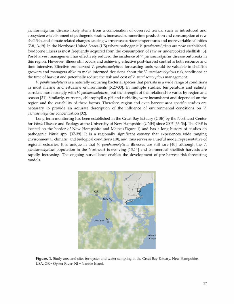
37

parahaemolyticus disease likely stems from a combination of observed trends, such as introduced and

ecosystem establishment of pathogenic strains, increased summertime production and consumption of raw

shellfish, and climate related changes causing warmer sea surface temperatures and more variable salinities

[7-8,13-19]. In the Northeast United States (US) where pathogenic V. parahaemolyticus are now established,

foodborne illness is most frequently acquired from the consumption of raw or undercooked shellfish [3].

Post-harvest management has effectively reduced the incidence of V. parahaemolyticus disease outbreaks in

this region. However, illness still occurs and achieving effective post-harvest control is both resource and

time intensive. Effective pre-harvest V. parahaemolyticus forecasting tools would be valuable to shellfish

growers and managers alike to make informed decisions about the V. parahaemolyticus risk conditions at

the time of harvest and potentially reduce the risk and cost of V. parahaemolyticus management.

V. parahaemolyticus is a naturally occurring bacterial species that persists in a wide range of conditions

in most marine and estuarine environments [5,20-30]. In multiple studies, temperature and salinity

correlate most strongly with V. parahaemolyticus, but the strength of this relationship varies by region and

season [31]. Similarly, nutrients, chlorophyll a, pH and turbidity, were inconsistent and depended on the

region and the variability of these factors. Therefore, region and even harvest area specific studies are

necessary to provide an accurate description of the influence of environmental conditions on V.

parahaemolyticus concentration [32].

Long-term monitoring has been established in the Great Bay Estuary (GBE) by the Northeast Center

for Vibrio Disease and Ecology at the University of New Hampshire (UNH) since 2007 [33-36]. The GBE is

located on the border of New Hampshire and Maine (Figure 1) and has a long history of studies on

pathogenic Vibrio spp. [37-39]. It is a regionally significant estuary that experiences wide ranging

environmental, climatic, and biological conditions [10], and thus serves as a useful model representative of

regional estuaries. It is unique in that V. parahaemolyticus illnesses are still rare [40], although the V.

parahaemolyticus population in the Northeast is evolving [13,14] and commercial shellfish harvests are

rapidly increasing. The ongoing surveillance enables the development of pre-harvest risk-forecasting

models.

Figure. 1. Study area and sites for oyster and water sampling in the Great Bay Estuary, New Hampshire,

USA. OR = Oyster River; NI = Nannie Island.

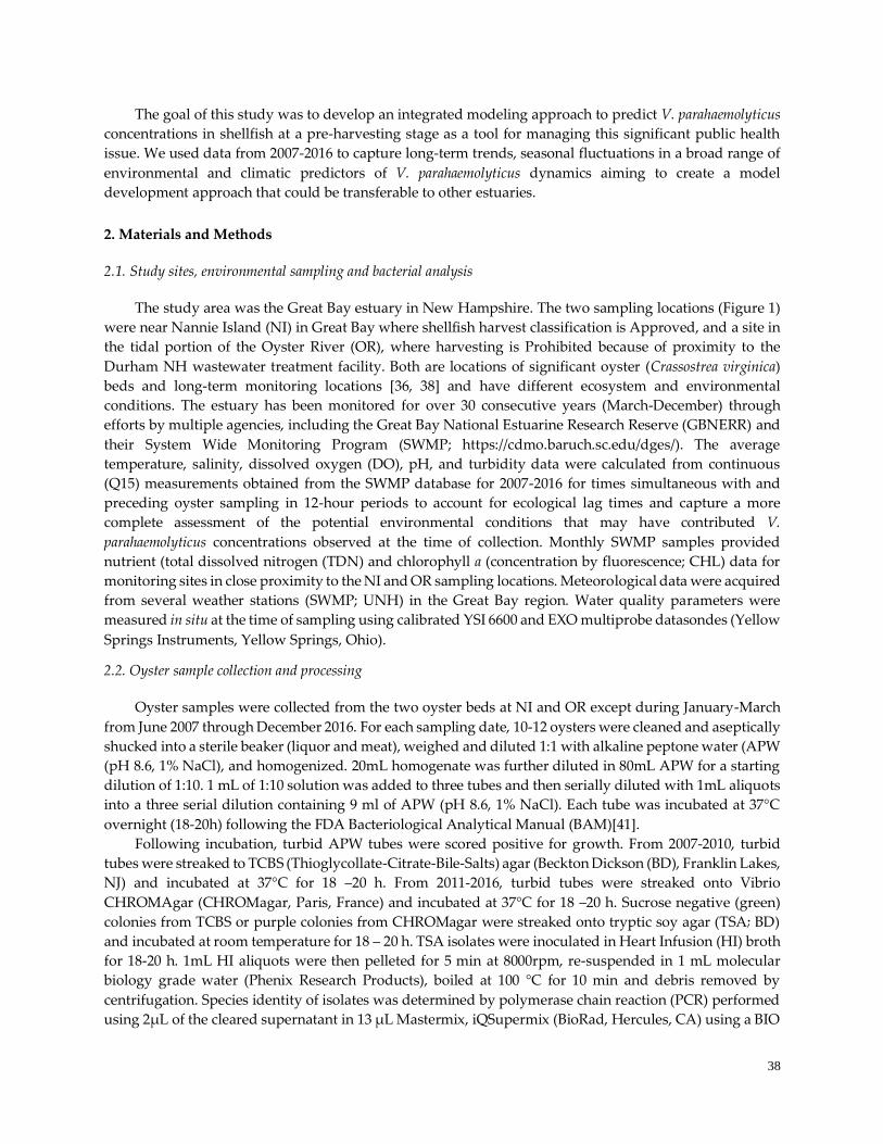
38

The goal of this study was to develop an integrated modeling approach to predict V. parahaemolyticus

concentrations in shellfish at a pre-harvesting stage as a tool for managing this significant public health

issue. We used data from 2007-2016 to capture long-term trends, seasonal fluctuations in a broad range of

environmental and climatic predictors of V. parahaemolyticus dynamics aiming to create a model

development approach that could be transferable to other estuaries.

2. Materials and Methods

2.1. Study sites, environmental sampling and bacterial analysis

The study area was the Great Bay estuary in New Hampshire. The two sampling locations (Figure 1)

were near Nannie Island (NI) in Great Bay where shellfish harvest classification is Approved, and a site in

the tidal portion of the Oyster River (OR), where harvesting is Prohibited because of proximity to the

Durham NH wastewater treatment facility. Both are locations of significant oyster (Crassostrea virginica)

beds and long-term monitoring locations [36, 38] and have different ecosystem and environmental

conditions. The estuary has been monitored for over 30 consecutive years (March-December) through

efforts by multiple agencies, including the Great Bay National Estuarine Research Reserve (GBNERR) and

their System Wide Monitoring Program (SWMP; https://cdmo.baruch.sc.edu/dges/). The average

temperature, salinity, dissolved oxygen (DO), pH, and turbidity data were calculated from continuous

(Q15) measurements obtained from the SWMP database for 2007-2016 for times simultaneous with and

preceding oyster sampling in 12-hour periods to account for ecological lag times and capture a more

complete assessment of the potential environmental conditions that may have contributed V.

parahaemolyticus concentrations observed at the time of collection. Monthly SWMP samples provided

nutrient (total dissolved nitrogen (TDN) and chlorophyll a (concentration by fluorescence; CHL) data for

monitoring sites in close proximity to the NI and OR sampling locations. Meteorological data were acquired

from several weather stations (SWMP; UNH) in the Great Bay region. Water quality parameters were

measured in situ at the time of sampling using calibrated YSI 6600 and EXO multiprobe datasondes (Yellow

Springs Instruments, Yellow Springs, Ohio).

2.2. Oyster sample collection and processing

Oyster samples were collected from the two oyster beds at NI and OR except during January-March

from June 2007 through December 2016. For each sampling date, 10-12 oysters were cleaned and aseptically

shucked into a sterile beaker (liquor and meat), weighed and diluted 1:1 with alkaline peptone water (APW

(pH 8.6, 1% NaCl), and homogenized. 20mL homogenate was further diluted in 80mL APW for a starting

dilution of 1:10. 1 mL of 1:10 solution was added to three tubes and then serially diluted with 1mL aliquots

into a three serial dilution containing 9 ml of APW (pH 8.6, 1% NaCl). Each tube was incubated at 37°C

overnight (18-20h) following the FDA Bacteriological Analytical Manual (BAM)[41].

Following incubation, turbid APW tubes were scored positive for growth. From 2007-2010, turbid

tubes were streaked to TCBS (Thioglycollate-Citrate-Bile-Salts) agar (Beckton Dickson (BD), Franklin Lakes,

NJ) and incubated at 37°C for 18 –20 h. From 2011-2016, turbid tubes were streaked onto Vibrio

CHROMAgar (CHROMagar, Paris, France) and incubated at 37°C for 18 –20 h. Sucrose negative (green)

colonies from TCBS or purple colonies from CHROMagar were streaked onto tryptic soy agar (TSA; BD)

and incubated at room temperature for 18 – 20 h. TSA isolates were inoculated in Heart Infusion (HI) broth

for 18-20 h. 1mL HI aliquots were then pelleted for 5 min at 8000rpm, re-suspended in 1 mL molecular

biology grade water (Phenix Research Products), boiled at 100 °C for 10 min and debris removed by

centrifugation. Species identity of isolates was determined by polymerase chain reaction (PCR) performed

using 2μL of the cleared supernatant in 13 μL Mastermix, iQSupermix (BioRad, Hercules, CA) using a BIO

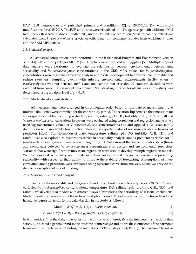
39

RAD T100 thermocycler and published primers and conditions [42] for 2007-2014; [19] with slight

modifications for 2015-2016. The PCR amplicons were visualized on 1.2% agarose gel with addition of Gel

Red (Phenix Research Products, Candler, NC) under UV light. Concentration (Most Probable Number) was

calculated from V. parahaemolyticus species-specific gene (tlh) confirmed isolates from enrichment tubes

and the BAM MPN tables.

2.3. Statistical analysis

All statistical computations were performed in the R Statistical Program and Environment, version

3.5.1 [43] with add-on packages MGCV [52]. Graphics were produced with ggplot2 [53]. Multiple steps of

data analysis were performed to evaluate the relationship between environmental determinants,

seasonality and V. parahaemolyticus concentrations in the GBE. MPN values for V. parahaemolyticus

concentrations were log-transformed for analysis and model development to approximate normality and

reduce skewness. Sampling events with missing environmental measurements (n=29), when V.

parahaemolyticus was not detected (n=71) and one sample that exceeded >2 standard deviations were

excluded from concentration model development. Statistical significance for all analysis in this study was

determined using an alpha level of p < 0.05.

2.3.1. Model development strategy

All measurements were arranged in chronological order based on the date of measurement and

multiple time series were compiled for the entire study period. The relationship between the time series for

water quality variables, including water temperature, salinity, pH, DO, turbidity, CHL, TDN, rainfall and

V. parahaemolyticus concentrations in oysters were evaluated using correlation and regression analysis. We

used log-transformed values of V. parahaemolyticus concentrations (Yt) and applied a Gaussian family

distribution with an identity link function relating the expected value of response variable Yt to selected

predictors [44,45]. Transformation of water temperature, salinity, pH, DO, turbidity, CHL, TDN and

rainfall was also explored as response variables in seasonality analysis and as predictor variables for V.

parahaemolyticus in regression analysis with log or log + 1. We assessed the shape of relationships (linear

and non-linear) between V. parahaemolyticus concentrations in oysters and environmental predictors.

Variables that were significant in univariate regression were used to develop multiple regression models.

We also assessed seasonality and trends over time and explored alternative variables representing

seasonality with respect to their ability to improve the stability of forecasting. Assumptions of inter-

correlation among predictors were evaluated using Spearman correlation analysis. Below we provide the

detailed description of model building.

2.3.2. Seasonality and trend analysis

To explore the seasonality and the general trend throughout the whole study period (2007-2016) in all

variables: V. parahaemolyticus concentrations, temperature, DO, salinity, pH, turbidity, CHL, TDN and

rainfall, we develop two models with different ways of presenting the periodicity of seasonal oscillations.

Model 1 contains variables for a linear trend and photoperiod. Model 2 uses terms for a linear trend and

harmonic regression terms for the calendar day in the study as follows:

Model 1: 𝐸(𝑌𝑡) = 𝛽0 + 𝛽1𝑡 + 𝛽p𝑃ℎ𝑜𝑡𝑜𝑝𝑒𝑟𝑖𝑜𝑑, (1)

Model 2: 𝐸(𝑌𝑡) = 𝛽0 + 𝛽1𝑡 + 𝛽𝑠 sin(2𝜋𝜔𝑡) + 𝛽𝑐 cos(2𝜋𝜔𝑡). (2)

In both models, 𝑌𝑡 is the daily time series for the outcome of interest, 𝛽0 is the intercept, t is the daily time

series, 𝛽1indicated a general trend in the outcome of interest; 𝛽𝑠 and 𝛽𝑐 are the coefficients of the harmonic

terms and ω is the term representing the annual cycle (365.25 days, ω=1/365.25). The harmonic terms in

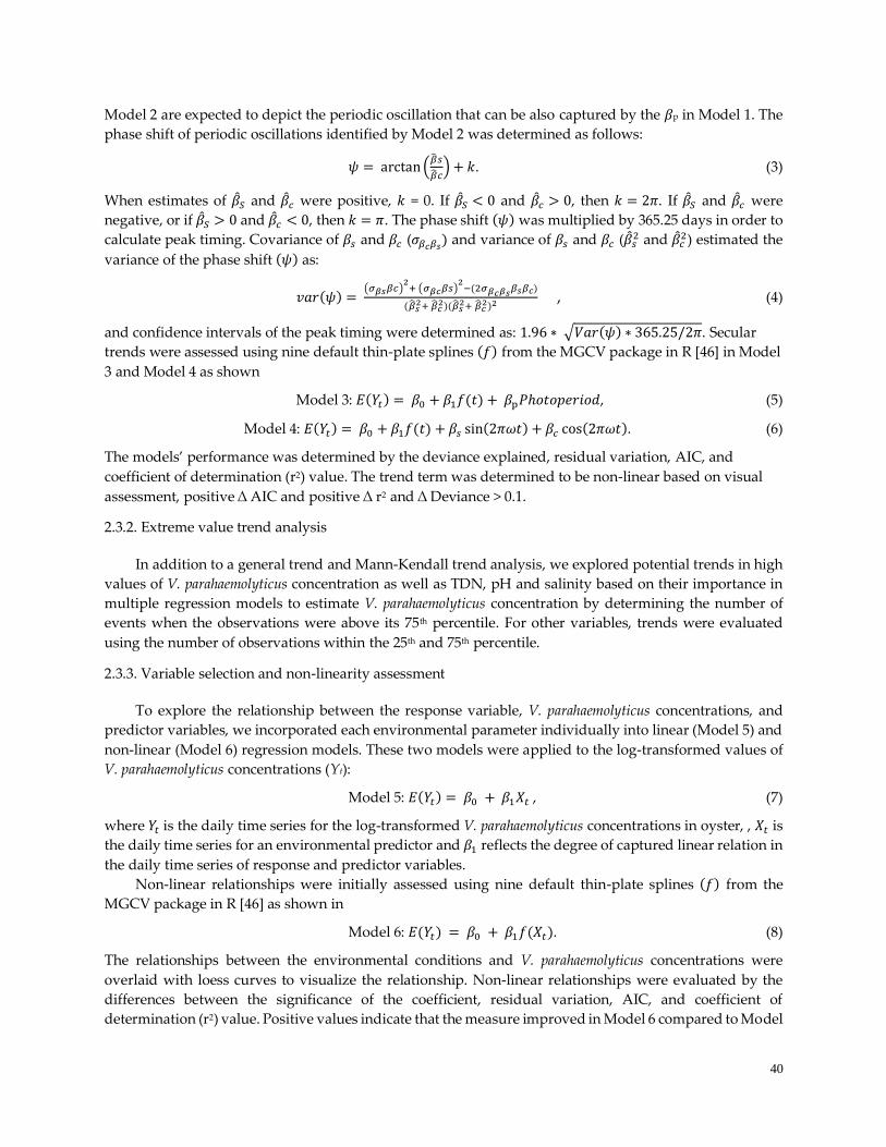
40

Model 2 are expected to depict the periodic oscillation that can be also captured by the 𝛽p in Model 1. The

phase shift of periodic oscillations identified by Model 2 was determined as follows:

𝜓 = arctan (𝑠

𝑐) + 𝑘. (3)

When estimates of 𝑆 and 𝑐 were positive, 𝑘 = 0. If 𝑆 < 0 and 𝑐 > 0, then 𝑘 = 2𝜋. If 𝑆 and 𝑐 were

negative, or if 𝑆 > 0 and 𝑐 < 0, then 𝑘 = 𝜋. The phase shift (𝜓) was multiplied by 365.25 days in order to

calculate peak timing. Covariance of 𝛽𝑠 and 𝛽𝑐 (𝜎𝛽𝑐𝛽𝑠) and variance of 𝛽𝑠 and 𝛽𝑐 (𝑠

2 and 𝑐2) estimated the

variance of the phase shift (𝜓) as:

𝑣𝑎𝑟(𝜓) = (𝜎𝛽𝑠𝛽𝑐)

2+ (𝜎𝛽𝑐𝛽𝑠)

2−(2𝜎𝛽𝑐𝛽𝑠

𝛽𝑠𝛽𝑐)

(𝑠2+ 𝑐

2)(𝑠2+ 𝑐

2)2 , (4)

and confidence intervals of the peak timing were determined as: 1.96 ∗ √𝑉𝑎𝑟(𝜓) ∗ 365.25/2𝜋. Secular

trends were assessed using nine default thin-plate splines (𝑓) from the MGCV package in R [46] in Model

3 and Model 4 as shown

Model 3: 𝐸(𝑌𝑡) = 𝛽0 + 𝛽1𝑓(𝑡) + 𝛽p𝑃ℎ𝑜𝑡𝑜𝑝𝑒𝑟𝑖𝑜𝑑, (5)

Model 4: 𝐸(𝑌𝑡) = 𝛽0 + 𝛽1𝑓(𝑡) + 𝛽𝑠 sin(2𝜋𝜔𝑡) + 𝛽𝑐 cos(2𝜋𝜔𝑡). (6)

The models’ performance was determined by the deviance explained, residual variation, AIC, and

coefficient of determination (r2) value. The trend term was determined to be non-linear based on visual

assessment, positive ∆ AIC and positive ∆ r2 and ∆ Deviance > 0.1.

2.3.2. Extreme value trend analysis

In addition to a general trend and Mann-Kendall trend analysis, we explored potential trends in high

values of V. parahaemolyticus concentration as well as TDN, pH and salinity based on their importance in

multiple regression models to estimate V. parahaemolyticus concentration by determining the number of

events when the observations were above its 75th percentile. For other variables, trends were evaluated

using the number of observations within the 25th and 75th percentile.

2.3.3. Variable selection and non-linearity assessment

To explore the relationship between the response variable, V. parahaemolyticus concentrations, and

predictor variables, we incorporated each environmental parameter individually into linear (Model 5) and

non-linear (Model 6) regression models. These two models were applied to the log-transformed values of

V. parahaemolyticus concentrations (Yt):

Model 5: 𝐸(𝑌𝑡) = 𝛽0 + 𝛽1𝑋𝑡 , (7)

where 𝑌𝑡 is the daily time series for the log-transformed V. parahaemolyticus concentrations in oyster, , 𝑋𝑡 is

the daily time series for an environmental predictor and 𝛽1 reflects the degree of captured linear relation in

the daily time series of response and predictor variables.

Non-linear relationships were initially assessed using nine default thin-plate splines (𝑓) from the

MGCV package in R [46] as shown in

Model 6: 𝐸(𝑌𝑡) = 𝛽0 + 𝛽1𝑓(𝑋𝑡). (8)

The relationships between the environmental conditions and V. parahaemolyticus concentrations were

overlaid with loess curves to visualize the relationship. Non-linear relationships were evaluated by the

differences between the significance of the coefficient, residual variation, AIC, and coefficient of

determination (r2) value. Positive values indicate that the measure improved in Model 6 compared to Model

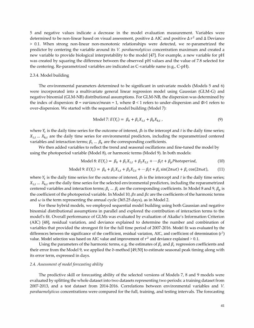
41

5 and negative values indicate a decrease in the model evaluation measurement. Variables were

determined to be non-linear based on visual assessment, positive ∆ AIC and positive ∆ 𝑟2 and ∆ Deviance

> 0.1. When strong non-linear non-monotonic relationships were detected, we re-parametrized the

predictor by centering the variable around its V. parahaemolyticus concentration maximum and created a

new variable to provide biological interpretability to the model [47]. For example, a new variable for pH

was created by squaring the difference between the observed pH values and the value of 7.8 selected for

the centering. Re-parametrized variables are indicated as C-variable name (e.g., C-pH).

2.3.4. Model building

The environmental parameters determined to be significant in univariate models (Models 5 and 6)

were incorporated into a multivariate general linear regression model using Gaussian (GLM-G) and

negative binomial (GLM-NB) distributional assumptions. For GLM-NB, the dispersion was determined by

the index of dispersion: ∅ = 𝑣𝑎𝑟𝑖𝑎𝑛𝑐𝑒/𝑚𝑒𝑎𝑛 = 1, where ∅ < 1 refers to under-dispersion and ∅>1 refers to

over-dispersion. We started with the sequential model building (Model 7):

Model 7: 𝐸(𝑌𝑡) = 𝛽0 + 𝛽1𝑋1,𝑡 + 𝛽k𝑋k,𝑡 , (9)

where 𝑌𝑡 is the daily time series for the outcome of interest, 𝛽0 is the intercept and t is the daily time series;

𝑋1,𝑡 … 𝑋k,𝑡 are the daily time series for environmental predictors, including the reparametrized centered

variables and interaction terms; 𝛽1 … 𝛽𝑘 are the corresponding coefficients.

We then added variables to reflect the trend and seasonal oscillations and fine-tuned the model by

using the photoperiod variable (Model 8), or harmonic terms (Model 9). In both models:

Model 8: 𝐸(𝑌𝑡) = 𝛽0 + 𝛽1𝑋1,𝑡 + 𝛽2𝑋2,𝑡 + ⋯ 𝛽𝑙𝑡 + 𝛽𝑝𝑃ℎ𝑜𝑡𝑜𝑝𝑒𝑟𝑖𝑜𝑑, (10)

Model 9: 𝐸(𝑌𝑡) = 𝛽0 + 𝛽1𝑋1,𝑡 + 𝛽2𝑋2,𝑡 + ⋯ 𝛽𝑙𝑡 + 𝛽𝑠 sin(2𝜋𝜔𝑡) + 𝛽𝑐 cos(2𝜋𝜔𝑡), (11)

where 𝑌𝑡 is the daily time series for the outcome of interest, 𝛽0 is the intercept and t is the daily time series;

𝑋1,𝑡 … 𝑋k,𝑡 are the daily time series for the selected environmental predictors, including the reparametrized

centered variables and interaction terms; 𝛽1 … 𝛽𝑙 are the corresponding coefficients. In Model 8 and 9, 𝛽p is

the coefficient of the photoperiod variable. In Model 10, 𝛽𝑠 and 𝛽𝑐 are the coefficients of the harmonic terms

and ω is the term representing the annual cycle (365.25 days), as in Model 2.

For these hybrid models, we employed sequential model building using both Gaussian and negative

binomial distributional assumptions in parallel and explored the contribution of interaction terms to the

model’s fit. Overall performance of GLMs was evaluated by evaluation of Akaike’s Information Criterion

(AIC) [48], residual variation, and deviance explained to determine the number and combination of

variables that provided the strongest fit for the full time period of 2007-2016. Model fit was evaluated by the

differences between the significance of the coefficient, residual variation, AIC, and coefficient of determination (r2)

value. Model selection was based on AIC value and improvement of 𝑟2 and deviance explained > 0.1. Using the parameters of the harmonic terms, e.g. the estimates of 𝛽𝑠 and 𝛽𝑐 regression coefficients and

their error from the Model 9, we applied the δ-method [49,50] to estimate seasonal peak timing along with

its error term, expressed in days.

2.4. Assessment of model forecasting ability

The predictive skill or forecasting ability of the selected versions of Models 7, 8 and 9 models were

evaluated by splitting the whole dataset into two datasets representing two periods: a training dataset from

2007-2013, and a test dataset from 2014-2016. Correlations between environmental variables and V.

parahaemolyticus concentrations were compared for the full, training, and testing intervals. The forecasting

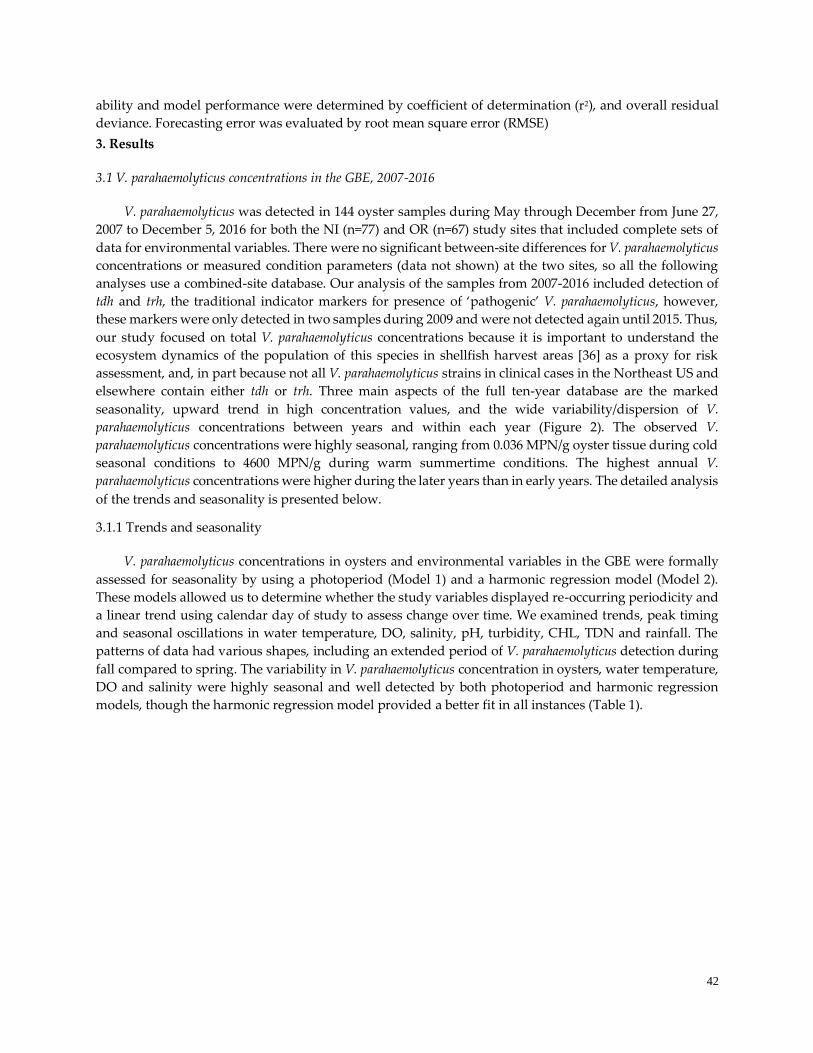
42

ability and model performance were determined by coefficient of determination (r2), and overall residual

deviance. Forecasting error was evaluated by root mean square error (RMSE)

3. Results

3.1 V. parahaemolyticus concentrations in the GBE, 2007-2016

V. parahaemolyticus was detected in 144 oyster samples during May through December from June 27,

2007 to December 5, 2016 for both the NI (n=77) and OR (n=67) study sites that included complete sets of

data for environmental variables. There were no significant between-site differences for V. parahaemolyticus

concentrations or measured condition parameters (data not shown) at the two sites, so all the following

analyses use a combined-site database. Our analysis of the samples from 2007-2016 included detection of

tdh and trh, the traditional indicator markers for presence of ‘pathogenic’ V. parahaemolyticus, however,

these markers were only detected in two samples during 2009 and were not detected again until 2015. Thus,

our study focused on total V. parahaemolyticus concentrations because it is important to understand the

ecosystem dynamics of the population of this species in shellfish harvest areas [36] as a proxy for risk

assessment, and, in part because not all V. parahaemolyticus strains in clinical cases in the Northeast US and

elsewhere contain either tdh or trh. Three main aspects of the full ten-year database are the marked

seasonality, upward trend in high concentration values, and the wide variability/dispersion of V.

parahaemolyticus concentrations between years and within each year (Figure 2). The observed V.

parahaemolyticus concentrations were highly seasonal, ranging from 0.036 MPN/g oyster tissue during cold

seasonal conditions to 4600 MPN/g during warm summertime conditions. The highest annual V.

parahaemolyticus concentrations were higher during the later years than in early years. The detailed analysis

of the trends and seasonality is presented below.

3.1.1 Trends and seasonality

V. parahaemolyticus concentrations in oysters and environmental variables in the GBE were formally

assessed for seasonality by using a photoperiod (Model 1) and a harmonic regression model (Model 2).

These models allowed us to determine whether the study variables displayed re-occurring periodicity and

a linear trend using calendar day of study to assess change over time. We examined trends, peak timing

and seasonal oscillations in water temperature, DO, salinity, pH, turbidity, CHL, TDN and rainfall. The

patterns of data had various shapes, including an extended period of V. parahaemolyticus detection during

fall compared to spring. The variability in V. parahaemolyticus concentration in oysters, water temperature,

DO and salinity were highly seasonal and well detected by both photoperiod and harmonic regression

models, though the harmonic regression model provided a better fit in all instances (Table 1).

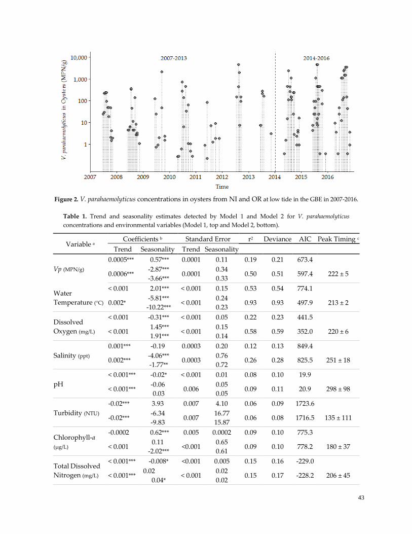
43

Figure 2. V. parahaemolyticus concentrations in oysters from NI and OR at low tide in the GBE in 2007-2016.

Table 1. Trend and seasonality estimates detected by Model 1 and Model 2 for V. parahaemolyticus

concentrations and environmental variables (Model 1, top and Model 2, bottom).

Variable a Coefficients b Standard Error r2 Deviance AIC Peak Timing c

Trend Seasonality Trend Seasonality

Vp (MPN/g)

0.0005*** 0.57*** 0.0001 0.11 0.19 0.21 673.4

0.0006*** -2.87***

-3.66*** 0.0001

0.34

0.33 0.50 0.51 597.4 222 ± 5

Water

Temperature (°C)

< 0.001 2.01*** < 0.001 0.15 0.53 0.54 774.1

0.002* -5.81***

-10.22*** < 0.001

0.24

0.23 0.93 0.93 497.9 213 ± 2

Dissolved

Oxygen (mg/L)

< 0.001 -0.31*** < 0.001 0.05 0.22 0.23 441.5

< 0.001 1.45***

1.91*** < 0.001

0.15

0.14 0.58 0.59 352.0 220 ± 6

Salinity (ppt)

0.001*** -0.19 0.0003 0.20 0.12 0.13 849.4

0.002*** -4.06***

-1.77** 0.0003

0.76

0.72 0.26 0.28 825.5 251 ± 18

pH

< 0.001*** -0.02* < 0.001 0.01 0.08 0.10 19.9

< 0.001*** -0.06

0.03 0.006

0.05

0.05 0.09 0.11 20.9 298 ± 98

Turbidity (NTU)

-0.02*** 3.93 0.007 4.10 0.06 0.09 1723.6

-0.02*** -6.34

-9.83 0.007

16.77

15.87 0.06 0.08 1716.5 135 ± 111

Chlorophyll-a

(µg/L)

-0.0002 0.62*** 0.005 0.0002 0.09 0.10 775.3

< 0.001 0.11

-2.02*** <0.001

0.65

0.61 0.09 0.10 778.2 180 ± 37

Total Dissolved

Nitrogen (mg/L)

< 0.001*** -0.008* <0.001 0.005 0.15 0.16 -229.0

< 0.001*** 0.02

0.04* < 0.001

0.02

0.02 0.15 0.17 -228.2 206 ± 45

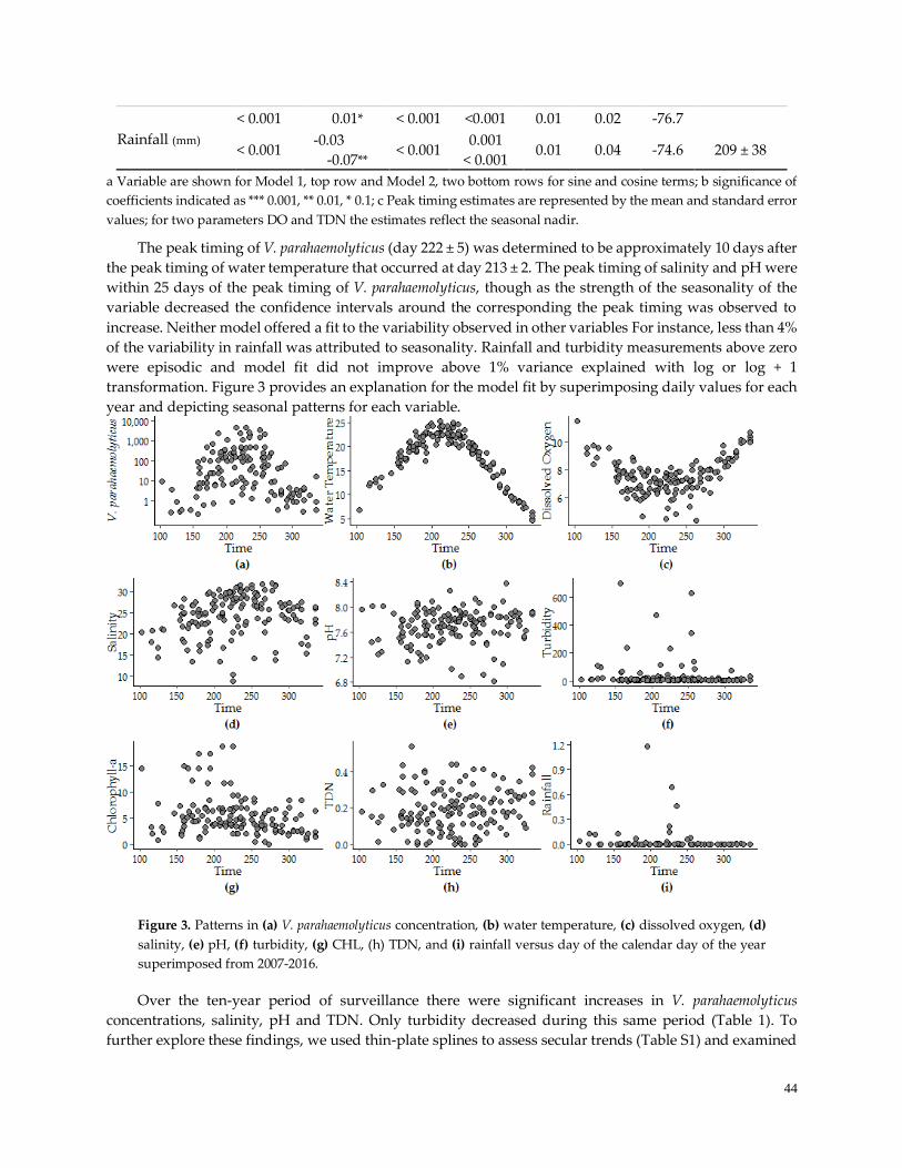
44

Rainfall (mm)

< 0.001 0.01* < 0.001 <0.001 0.01 0.02 -76.7

< 0.001 -0.03

-0.07** < 0.001

0.001

< 0.001 0.01 0.04 -74.6 209 ± 38

a Variable are shown for Model 1, top row and Model 2, two bottom rows for sine and cosine terms; b significance of

coefficients indicated as *** 0.001, ** 0.01, * 0.1; c Peak timing estimates are represented by the mean and standard error

values; for two parameters DO and TDN the estimates reflect the seasonal nadir.

The peak timing of V. parahaemolyticus (day 222 ± 5) was determined to be approximately 10 days after

the peak timing of water temperature that occurred at day 213 ± 2. The peak timing of salinity and pH were

within 25 days of the peak timing of V. parahaemolyticus, though as the strength of the seasonality of the

variable decreased the confidence intervals around the corresponding the peak timing was observed to

increase. Neither model offered a fit to the variability observed in other variables For instance, less than 4%

of the variability in rainfall was attributed to seasonality. Rainfall and turbidity measurements above zero

were episodic and model fit did not improve above 1% variance explained with log or log + 1

transformation. Figure 3 provides an explanation for the model fit by superimposing daily values for each

year and depicting seasonal patterns for each variable.

Figure 3. Patterns in (a) V. parahaemolyticus concentration, (b) water temperature, (c) dissolved oxygen, (d)

salinity, (e) pH, (f) turbidity, (g) CHL, (h) TDN, and (i) rainfall versus day of the calendar day of the year

superimposed from 2007-2016.

Over the ten-year period of surveillance there were significant increases in V. parahaemolyticus

concentrations, salinity, pH and TDN. Only turbidity decreased during this same period (Table 1). To

further explore these findings, we used thin-plate splines to assess secular trends (Table S1) and examined

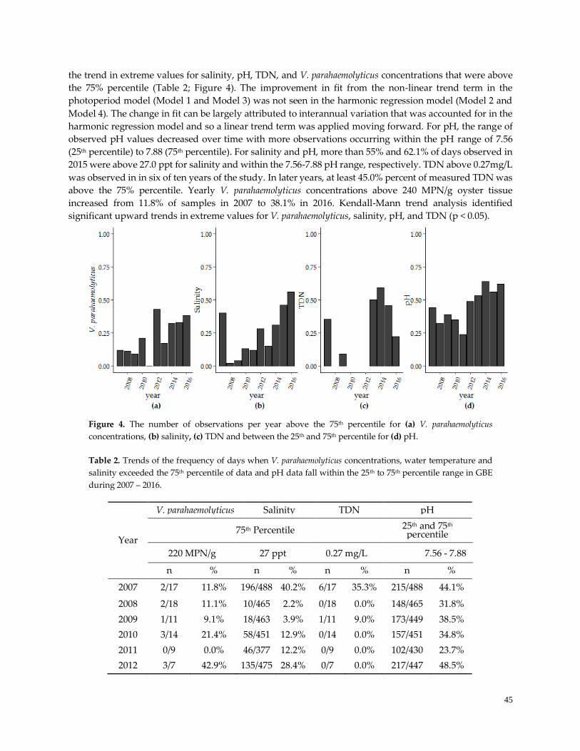
45

the trend in extreme values for salinity, pH, TDN, and V. parahaemolyticus concentrations that were above

the 75% percentile (Table 2; Figure 4). The improvement in fit from the non-linear trend term in the

photoperiod model (Model 1 and Model 3) was not seen in the harmonic regression model (Model 2 and

Model 4). The change in fit can be largely attributed to interannual variation that was accounted for in the

harmonic regression model and so a linear trend term was applied moving forward. For pH, the range of

observed pH values decreased over time with more observations occurring within the pH range of 7.56

(25th percentile) to 7.88 (75th percentile). For salinity and pH, more than 55% and 62.1% of days observed in

2015 were above 27.0 ppt for salinity and within the 7.56-7.88 pH range, respectively. TDN above 0.27mg/L

was observed in in six of ten years of the study. In later years, at least 45.0% percent of measured TDN was

above the 75% percentile. Yearly V. parahaemolyticus concentrations above 240 MPN/g oyster tissue

increased from 11.8% of samples in 2007 to 38.1% in 2016. Kendall-Mann trend analysis identified

significant upward trends in extreme values for V. parahaemolyticus, salinity, pH, and TDN (p < 0.05).

Figure 4. The number of observations per year above the 75th percentile for (a) V. parahaemolyticus

concentrations, (b) salinity, (c) TDN and between the 25th and 75th percentile for (d) pH.

Table 2. Trends of the frequency of days when V. parahaemolyticus concentrations, water temperature and

salinity exceeded the 75th percentile of data and pH data fall within the 25th to 75th percentile range in GBE

during 2007 – 2016.

Year

V. parahaemolyticus Salinity TDN pH

75th Percentile 25th and 75th percentile

220 MPN/g 27 ppt 0.27 mg/L 7.56 - 7.88

n % n % n % n %

2007 2/17 11.8% 196/488 40.2% 6/17 35.3% 215/488 44.1%

2008 2/18 11.1% 10/465 2.2% 0/18 0.0% 148/465 31.8%

2009 1/11 9.1% 18/463 3.9% 1/11 9.0% 173/449 38.5%

2010 3/14 21.4% 58/451 12.9% 0/14 0.0% 157/451 34.8%

2011 0/9 0.0% 46/377 12.2% 0/9 0.0% 102/430 23.7%

2012 3/7 42.9% 135/475 28.4% 0/7 0.0% 217/447 48.5%

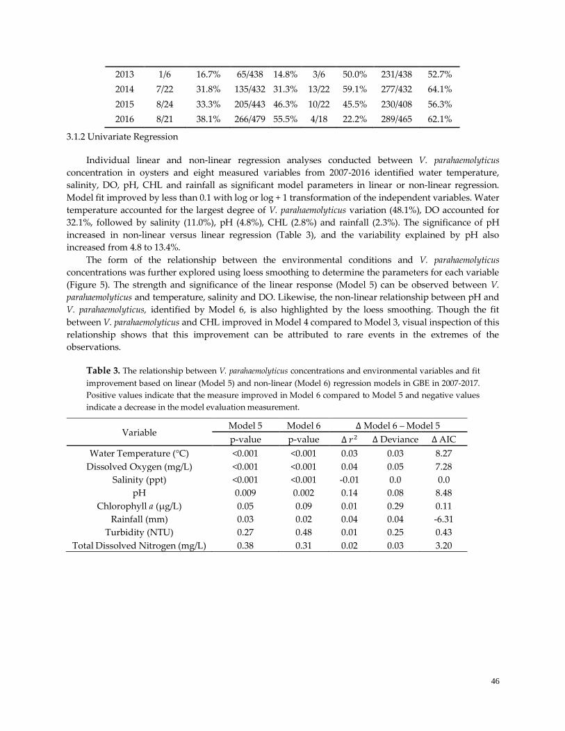
46

2013 1/6 16.7% 65/438 14.8% 3/6 50.0% 231/438 52.7%

2014 7/22 31.8% 135/432 31.3% 13/22 59.1% 277/432 64.1%

2015 8/24 33.3% 205/443 46.3% 10/22 45.5% 230/408 56.3%

2016 8/21 38.1% 266/479 55.5% 4/18 22.2% 289/465 62.1%

3.1.2 Univariate Regression

Individual linear and non-linear regression analyses conducted between V. parahaemolyticus

concentration in oysters and eight measured variables from 2007-2016 identified water temperature,

salinity, DO, pH, CHL and rainfall as significant model parameters in linear or non-linear regression.

Model fit improved by less than 0.1 with log or log + 1 transformation of the independent variables. Water

temperature accounted for the largest degree of V. parahaemolyticus variation (48.1%), DO accounted for

32.1%, followed by salinity (11.0%), pH (4.8%), CHL (2.8%) and rainfall (2.3%). The significance of pH

increased in non-linear versus linear regression (Table 3), and the variability explained by pH also

increased from 4.8 to 13.4%.

The form of the relationship between the environmental conditions and V. parahaemolyticus

concentrations was further explored using loess smoothing to determine the parameters for each variable

(Figure 5). The strength and significance of the linear response (Model 5) can be observed between V.

parahaemolyticus and temperature, salinity and DO. Likewise, the non-linear relationship between pH and

V. parahaemolyticus, identified by Model 6, is also highlighted by the loess smoothing. Though the fit

between V. parahaemolyticus and CHL improved in Model 4 compared to Model 3, visual inspection of this

relationship shows that this improvement can be attributed to rare events in the extremes of the

observations.

Table 3. The relationship between V. parahaemolyticus concentrations and environmental variables and fit

improvement based on linear (Model 5) and non-linear (Model 6) regression models in GBE in 2007-2017.

Positive values indicate that the measure improved in Model 6 compared to Model 5 and negative values

indicate a decrease in the model evaluation measurement.

Variable Model 5 Model 6 ∆ Model 6 – Model 5

p-value p-value ∆ 𝑟2 ∆ Deviance ∆ AIC

Water Temperature (°C) <0.001 <0.001 0.03 0.03 8.27

Dissolved Oxygen (mg/L) <0.001 <0.001 0.04 0.05 7.28

Salinity (ppt) <0.001 <0.001 -0.01 0.0 0.0

pH 0.009 0.002 0.14 0.08 8.48

Chlorophyll a (µg/L) 0.05 0.09 0.01 0.29 0.11

Rainfall (mm) 0.03 0.02 0.04 0.04 -6.31

Turbidity (NTU) 0.27 0.48 0.01 0.25 0.43

Total Dissolved Nitrogen (mg/L) 0.38 0.31 0.02 0.03 3.20

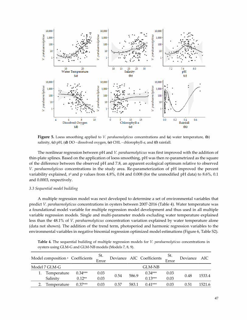
47

Figure 5. Loess smoothing applied to V. parahaemolyticus concentrations and (a) water temperature, (b)

salinity, (c) pH, (d) DO - dissolved oxygen, (e) CHL - chlorophyll-a, and (f) rainfall.

The nonlinear regression between pH and V. parahaemolyticus was first improved with the addition of

thin-plate splines. Based on the application of loess smoothing, pH was then re-parametrized as the square

of the difference between the observed pH and 7.8, an apparent ecological optimum relative to observed

V. parahaemolyticus concentrations in the study area. Re-parameterization of pH improved the percent

variability explained, r2 and p values from 4.8%, 0.04 and 0.008 (for the unmodified pH data) to 8.6%, 0.1

and 0.0003, respectively.

3.3 Sequential model building

A multiple regression model was next developed to determine a set of environmental variables that

predict V. parahaemolyticus concentrations in oysters between 2007-2016 (Table 4). Water temperature was

a foundational model variable for multiple regression model development and thus used in all multiple

variable regression models. Single and multi-parameter models excluding water temperature explained

less than the 48.1% of V. parahaemolyticus concentration variation explained by water temperature alone

(data not shown). The addition of the trend term, photoperiod and harmonic regression variables to the

environmental variables in negative binomial regression optimized model estimations (Figure 6, Table S2).

Table 4. The sequential building of multiple regression models for V. parahaemolyticus concentrations in

oysters using GLM-G and GLM-NB models (Models 7, 8, 9).

Model composition a Coefficients St.

Error Deviance AIC Coefficients

St.

Error Deviance AIC

Model 7 GLM-G GLM-NB

1. Temperature

Salinity

0.34***

0.12**

0.03

0.03 0.54 586.9

0.34***

0.13***

0.03

0.03 0.48 1533.4

2. Temperature 0.37*** 0.03 0.57 583.1 0.41*** 0.03 0.51 1521.6

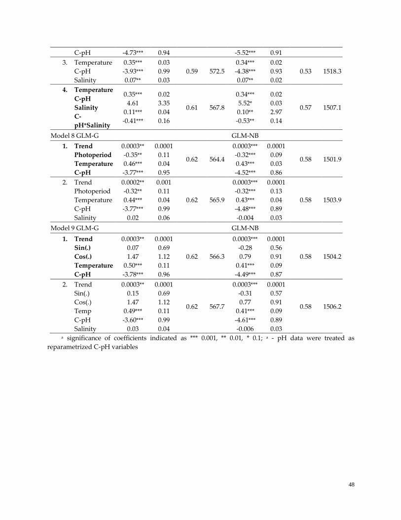
48

C-pH -4.73*** 0.94 -5.52*** 0.91

3. Temperature

C-pH

Salinity

0.35***

-3.93***

0.07**

0.03

0.99

0.03

0.59 572.5

0.34***

-4.38***

0.07**

0.02

0.93

0.02

0.53 1518.3

4. Temperature

C-pH

Salinity

C-

pH*Salinity

0.35***

4.61

0.11***

-0.41***

0.02

3.35

0.04

0.16

0.61 567.8

0.34***

5.52*

0.10**

-0.53**

0.02

0.03

2.97

0.14

0.57 1507.1


1. Trend

Photoperiod

Temperature

C-pH

0.0003**

-0.35**

0.46***

-3.77***

0.0001

0.11

0.04

0.95

0.62 564.4

0.0003***

-0.32***

0.43***

-4.52***

0.0001

0.09

0.03

0.86

0.58 1501.9

2. Trend

Photoperiod

Temperature

C-pH

Salinity

0.0002**

-0.32**

0.44***

-3.77***

0.02

0.001

0.11

0.04

0.99

0.06

0.62 565.9

0.0003***

-0.32***

0.43***

-4.48***

-0.004

0.0001

0.13

0.04

0.89

0.03

0.58 1503.9


1. Trend

Sin(.)

Cos(.)

Temperature

C-pH

0.0003**

0.07

1.47

0.50***

-3.78***

0.0001

0.69

1.12

0.11

0.96

0.62 566.3

0.0003***

-0.28

0.79

0.41***

-4.49***

0.0001

0.56

0.91

0.09

0.87

0.58 1504.2

2. Trend

Sin(.)

Cos(.)

Temp

C-pH

Salinity

0.0003**

0.15

1.47

0.49***

-3.60***

0.03

0.0001

0.69

1.12

0.11

0.99

0.04

0.62 567.7

0.0003***

-0.31

0.77

0.41***

-4.61***

-0.006

0.0001

0.57

0.91

0.09

0.89

0.03

0.58 1506.2

a significance of coefficients indicated as *** 0.001, ** 0.01, * 0.1; a - pH data were treated as

reparametrized C-pH variables

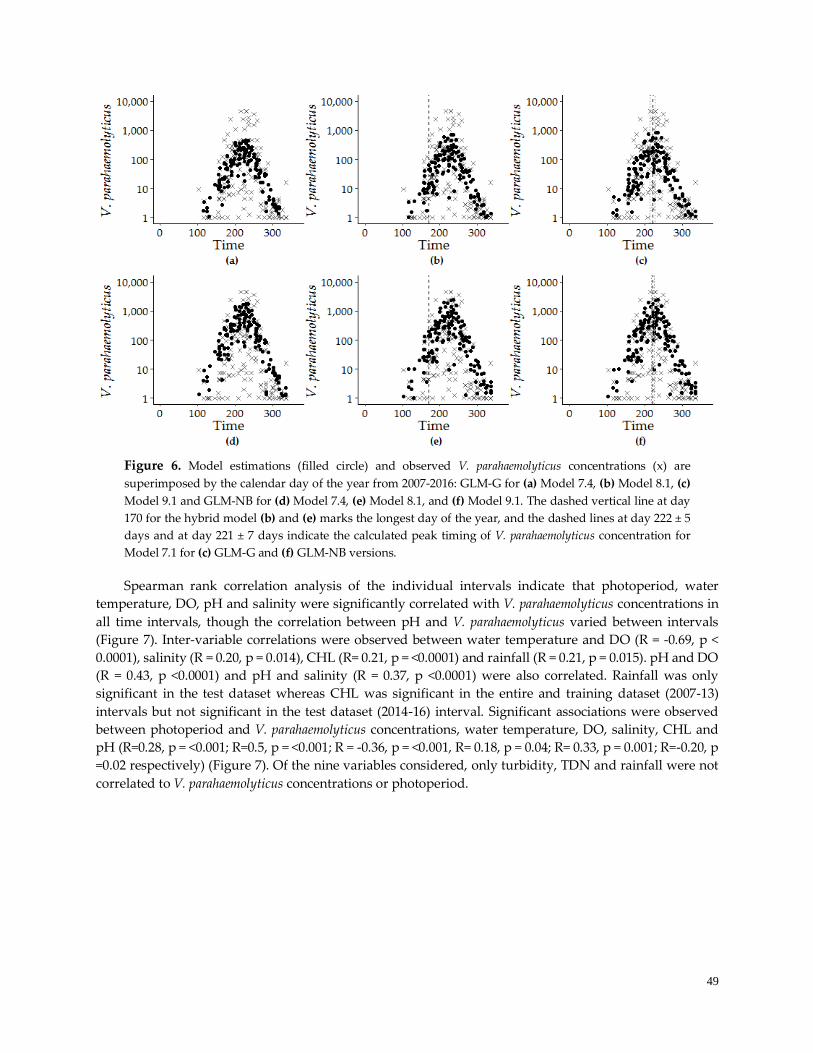
49

Figure 6. Model estimations (filled circle) and observed V. parahaemolyticus concentrations (x) are

superimposed by the calendar day of the year from 2007-2016: GLM-G for (a) Model 7.4, (b) Model 8.1, (c)

Model 9.1 and GLM-NB for (d) Model 7.4, (e) Model 8.1, and (f) Model 9.1. The dashed vertical line at day

170 for the hybrid model (b) and (e) marks the longest day of the year, and the dashed lines at day 222 ± 5

days and at day 221 ± 7 days indicate the calculated peak timing of V. parahaemolyticus concentration for

Model 7.1 for (c) GLM-G and (f) GLM-NB versions.

Spearman rank correlation analysis of the individual intervals indicate that photoperiod, water

temperature, DO, pH and salinity were significantly correlated with V. parahaemolyticus concentrations in

all time intervals, though the correlation between pH and V. parahaemolyticus varied between intervals

(Figure 7). Inter-variable correlations were observed between water temperature and DO (R = -0.69, p <

0.0001), salinity (R = 0.20, p = 0.014), CHL (R= 0.21, p = <0.0001) and rainfall (R = 0.21, p = 0.015). pH and DO

(R = 0.43, p <0.0001) and pH and salinity (R = 0.37, p <0.0001) were also correlated. Rainfall was only

significant in the test dataset whereas CHL was significant in the entire and training dataset (2007-13)

intervals but not significant in the test dataset (2014-16) interval. Significant associations were observed

between photoperiod and V. parahaemolyticus concentrations, water temperature, DO, salinity, CHL and

pH (R=0.28, p = <0.001; R=0.5, p = <0.001; R = -0.36, p = <0.001, R= 0.18, p = 0.04; R= 0.33, p = 0.001; R=-0.20, p

=0.02 respectively) (Figure 7). Of the nine variables considered, only turbidity, TDN and rainfall were not

correlated to V. parahaemolyticus concentrations or photoperiod.

50

Figure 7. Spearman correlation analysis of V. parahaemolyticus concentrations and environmental variables

for three intervals: (a) 2007-2016, (b) 2007-2013 and (c) 2014-2016. Red indicates positive and blue negative

correlations and the degree of significance is highlighted by color intensity.

3.4 Model Performance-Prediction

The hybrid model (Model 9.1) provided the best overall fit for each dataset time interval with

consistently lower RMSE and higher r2 values compared to the harmonic regression (Model 10.1) and

environmental model (Model 7.4) (Table 5). The fits for all three models were relatively consistent even

though the significance of some variables changed between time intervals. Although the estimations of

precision for the harmonic regression model across training/test datasets were slightly lower than for other

models, it is advantageous because important attributes of the data can be identified. For example, the V.

parahaemolyticus concentrations peaked on 222 ± 5 day of the 365.25-day period for all three intervals.

Similarly, the peak timing of water temperature and salinity were stable between the overall, training and

test data sets (212 ± 2 day and 251 ± 18 day, respectively).

Table 5. The performance of three selected models: environmental model (Model 7.4), hybrid model (Model

8.1), and harmonic regression (Model 9.1) for three time periods: full (P1), training (P2), and testing (P3)

intervals.

Model Variable a Time Interval

P1 P2 P3

Model 7.4 Coefficient: Temperature 0.34*** 0.37*** 0.31***

Salinity 0.10*** 0.08** 0.24**

C-pH 5.51* 5.12 266.01***

Salinity*C-pH -0.53*** -0.53*** -11.01***

r2 0.54 0.58 0.57

Deviance 0.57 0.58 0.54

RMSE 1.91 1.79 1.96

Model 8.1 Coefficient: Trend 0.0003*** 0.0003 0.0007

Photoperiod -0.31*** -0.28** -0.48**

Temperature 0.43*** 0.45*** 0.44***

C-pH -4.51*** -4.32*** -5.10

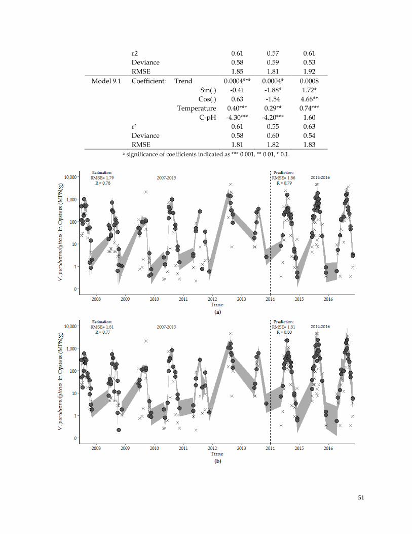
51

r2 0.61 0.57 0.61

Deviance 0.58 0.59 0.53

RMSE 1.85 1.81 1.92

Model 9.1 Coefficient: Trend 0.0004*** 0.0004* 0.0008

Sin(.) -0.41 -1.88* 1.72*

Cos(.) 0.63 -1.54 4.66**

Temperature 0.40*** 0.29** 0.74***

C-pH -4.30*** -4.20*** 1.60

r2 0.61 0.55 0.63

Deviance 0.58 0.60 0.54

RMSE 1.81 1.82 1.83 a significance of coefficients indicated as *** 0.001, ** 0.01, * 0.1.

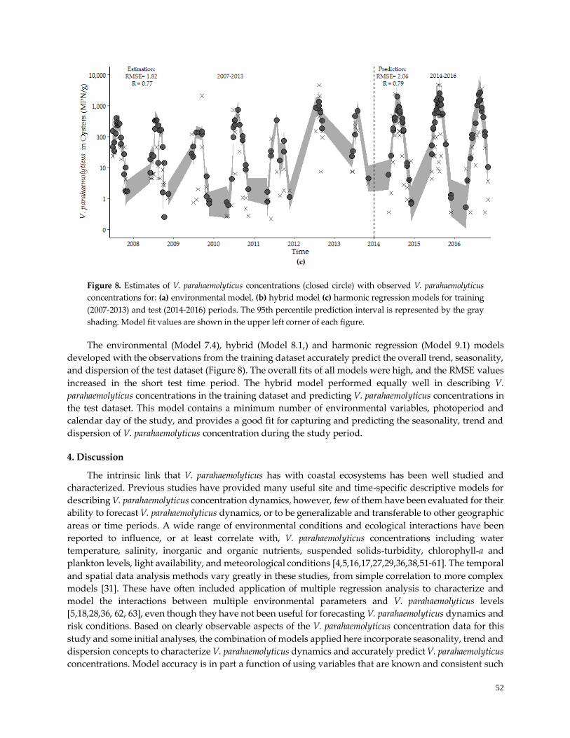
52

Figure 8. Estimates of V. parahaemolyticus concentrations (closed circle) with observed V. parahaemolyticus

concentrations for: (a) environmental model, (b) hybrid model (c) harmonic regression models for training

(2007-2013) and test (2014-2016) periods. The 95th percentile prediction interval is represented by the gray

shading. Model fit values are shown in the upper left corner of each figure.

The environmental (Model 7.4), hybrid (Model 8.1,) and harmonic regression (Model 9.1) models

developed with the observations from the training dataset accurately predict the overall trend, seasonality,

and dispersion of the test dataset (Figure 8). The overall fits of all models were high, and the RMSE values

increased in the short test time period. The hybrid model performed equally well in describing V.

parahaemolyticus concentrations in the training dataset and predicting V. parahaemolyticus concentrations in

the test dataset. This model contains a minimum number of environmental variables, photoperiod and

calendar day of the study, and provides a good fit for capturing and predicting the seasonality, trend and

dispersion of V. parahaemolyticus concentration during the study period.

4. Discussion

The intrinsic link that V. parahaemolyticus has with coastal ecosystems has been well studied and

characterized. Previous studies have provided many useful site and time-specific descriptive models for

describing V. parahaemolyticus concentration dynamics, however, few of them have been evaluated for their

ability to forecast V. parahaemolyticus dynamics, or to be generalizable and transferable to other geographic

areas or time periods. A wide range of environmental conditions and ecological interactions have been

reported to influence, or at least correlate with, V. parahaemolyticus concentrations including water

temperature, salinity, inorganic and organic nutrients, suspended solids-turbidity, chlorophyll-a and

plankton levels, light availability, and meteorological conditions [4,5,16,17,27,29,36,38,51-61]. The temporal

and spatial data analysis methods vary greatly in these studies, from simple correlation to more complex

models [31]. These have often included application of multiple regression analysis to characterize and

model the interactions between multiple environmental parameters and V. parahaemolyticus levels

[5,18,28,36, 62, 63], even though they have not been useful for forecasting V. parahaemolyticus dynamics and

risk conditions. Based on clearly observable aspects of the V. parahaemolyticus concentration data for this

study and some initial analyses, the combination of models applied here incorporate seasonality, trend and

dispersion concepts to characterize V. parahaemolyticus dynamics and accurately predict V. parahaemolyticus

concentrations. Model accuracy is in part a function of using variables that are known and consistent such

53

as photoperiod or day of the year that are ecologically interpretable, but stable for effective V.

parahaemolyticus forecasting. This approach of seasonality and trend analysis has the potential to be

transferable for developing similar forecasting models patterns of V. parahaemolyticus dynamics in other

locations.

V. parahaemolyticus concentrations in the GBE during this study followed the same pattern each year

as concentrations increased rapidly each springtime as water temperatures increased, and after peak

concentrations during the warmest summer conditions, decreased as water temperatures decreased in the

fall each year. Such seasonality, where regular and predictable changes in environmental and climatic

conditions re-occur every calendar year, tends to become more pronounced with increasing distance from

the equator and is largely due to extreme temperature variation driven by variable photoperiod [64]. Water

temperature accounted for approximately 48.1% of the variation observed in V. parahaemolyticus

concentrations in this study, similar to what has been observed globally and especially in highly seasonal,

temperate water regions [27, 28, 59]. Thus, seasonality is a significant aspect of V. parahaemolyticus

concentration dynamics in temperate coastal areas like New Hampshire and the Northeast US.

Photoperiod and harmonic regression models along with correlation analysis showed that V.

parahaemolyticus concentration, water temperature, dissolved oxygen, pH, salinity and chlorophyll-a are

significantly related to variables that mirror seasonal patterns in the GBE. Likewise, these variables

accurately estimate V. parahaemolyticus concentrations in oysters. The synchronized seasonal periodic

oscillation is one probable explanation for why regression modeling favors water temperature as the most

significant model parameter. A complex combination of biological and physical environmental variables

certainly drives V. parahaemolyticus population dynamics, however, many of these environmental variables

are, in turn, driven mainly by seasonal temperature. Therefore, the variability they contribute to V.

parahaemolyticus concentrations is not significantly different than what is provided by water temperature.

For example, dissolved oxygen was negatively correlated with V. parahaemolyticus concentrations, similar

to what has been previously reported [20] and was the second strongest variable, estimating over 32% of

the variability in V. parahaemolyticus over the course of the study in the GBE. Since V. parahaemolyticus is a

facultative anaerobe, this finding has the potential to elucidate important biological dimensions of the

ecology of V. parahaemolyticus. Water temperature is a dominant driver of dissolved oxygen concentrations

so collinearity between these variables is likely. In addition, because of the constraints of mathematical

modeling, well-fit models are not necessarily mechanistically or ecologically descriptive [65], and in this

case, dissolved oxygen was omitted from model development to avoid multicollinearity in favor of water

temperature as a stronger model variable.

Salinity and water temperature are both seasonally variable parameters that, together are the most

commonly cited environmental drivers of V. parahaemolyticus concentration variation [16, 31, 66]. Salinity

was a significant predictive parameter for V. parahaemolyticus concentration in this study, though the

significance of salinity was dependent on the time interval (2007-2013 versus 2014-2016) of the data and the

trend adjustment in the model (Table S2). This type of variability has also been observed in risk assessment

[67, 68] and in previous studies where salinity sometimes shows a strong positive correlation with V.

parahaemolyticus [5,6,25, 62], whereas for others [28, 52, 59, 69], salinity and V. parahaemolyticus dynamics do

not correlate. Thus, the finding that salinity and other variables reported to be significant in other V.

parahaemolyticus concentration models were not included in this study’s final model may be, at least in part,

a function of both the specific conditions at this study site and time period and a function of the in-depth

statistical approach used.

Though most studies find little to no correlation between pH and V. parahaemolyticus concentration

[20,21,28], non-linear regression and correlation analysis identified pH as an important parameter for the

predictive models in the GBE. Loess smoothing highlighted the marked non-linearity of the relationship

between pH and V. parahaemolyticus concentrations and suggested a biological optimum/optimal range for

pH where V. parahaemolyticus concentrations decreased as pH increased or decreased relative to pH 7.8. For

54

the purposes of optimal model development, a new pH variable was constructed by reparametrizing the

measurements to create a linear response in V. parahaemolyticus as pH measurements moved from the

optima of 7.8. An optimal pH of 7.8 is near the pH (8.5) of alkaline peptone water medium used to optimally

enrich for Vibrio species [41] and has also been suggested as an optimal pH by laboratory-based

observations [70]. Wong et al., (1998) [71] found that exposure to more acidic environments tended to

reduce cell density and cause stress responses in V. parahaemolyticus. In this study, we observe that pH

measurements in the GBE appeared to become less variable and more basic in recent years, which was also

reported by Lopez-Hernandez et al., (2015)[5]. Thus, going beyond simple linear regression and including

the use of non-linear analysis reveals pH as an important and ecologically linked variable to explain V.

parahaemolyticus population dynamics.

In other studies [36,59, 62], variables other than salinity and pH were significant for estimating V.

parahaemolyticus concentrations in univariate regression, however in this study they provided an

insignificant amount of improvement to a multiple regression model that included water temperature. For

example, chlorophyll-a, considered a proxy measurement for phytoplankton abundance [21,31], was

significantly related to V. parahaemolyticus concentrations in correlation and univariate regression, but it

was not significant in a multiple regression model that included water temperature. Chlorophyll-a was

thus omitted from further model development because it did not contribute additional information in

describing V. parahaemolyticus variation. Many studies have suggested an important ecological interaction

between V. parahaemolyticus and plankton [27,54, 56, 62,68,72,73], and though chlorophyll-a was not

included in the multiple regression models, we have also conducted a parallel study to explore the

relationship between V. parahaemolyticus and plankton species across several years in the GBE [74,75] to

determine covarying plankton species. These have included phytoplankton that have been reported to be

significantly associated with V. parahaemolyticus elsewhere [76,77] that could provide more in-depth insight

into the importance of phytoplankton and the proxy chlorophyll-a to the V. parahaemolyticus concentration

dynamics observed in the GBE.

Approximately half of the variability of V. parahaemolyticus in the GBE could be predicted using the

contribution of photoperiod (in hours), sine and cosine of the day of the study in harmonic regression, and

the day of the study. Even though the model consisting solely of environmental variables was potentially

more ecologically informative, the trend and seasonality variables of calendar day of the study,

photoperiod, sine and cosine were more stable to estimate and predict the patterns of seasonality and trend

of increasingly high concentrations over time in V. parahaemolyticus than salinity and to a lesser degree pH

and do not require in situ measurements. Additionally, evaluation of the environmental model for its

forecasting ability highlighted that some evaluation measures were discordant, whereas the harmonic

regression and photoperiod model goodness-of-fit and forecasting error were in agreement. This highlights

that though multiple evaluation measures can cause complexities in model selection, in this study the

model with conflicting evaluation measures may indicate underlying issues, whereas the models where

evaluation measurements were in agreement provided stronger prediction accuracy. Harmonic regression

analyses also lead to identification of the day of year for peak V. parahaemolyticus concentration that occurs

in mid-August (day 222 ± 5 days) that followed the peak timing of water temperature (213 ± 2), whereas

the longest day of the year is June 21st (day 170). This highlights a loading, or hysteresis in the system and

provides the basis for understanding the ‘fall shoulder’ of elevated concentrations of V. parahaemolyticus

that extend into the late September.

Peak timing was used to assess each environmental variable individually to detect how environmental

variables may contribute to the development of ideal conditions for V. parahaemolyticus. Data in this study

were collected either monthly or biweekly, whereas V. parahaemolyticus replicates every eight minutes

under ideal conditions. In this instance, accurate detection of lagged effects on V. parahaemolyticus would

require more frequent sampling and fine-scale temporal resolution. Due to this level of biological

complexity and the irregular temporal intervals of the data in our study, the mean from 12 hours

55

proceeding collection was used for regression with environmental variables and peak timing was used to

assess temporally how each environmental variable may contribute to the development of ideal conditions

for V. parahaemolyticus. Using this approach, we determined that significant predictive variables peak in

advance of V. parahaemolyticus potentially contributing to a hysteresis or loading of the systems, setting up

conditions that are optimal for V. parahaemolyticus. Davis et al., 2019 [78] recently reported that

environmental variables approximately one month proceeding collection were significant to predicting V.

parahaemolyticus concentrations in the Chesapeake Bay suggesting they might also be observing this type

of lagged effect from a loading of the system. The application of harmonic regression and peak timing here

demonstrates how biological complexities and limitations of sampling frequency necessary can be

overcome whereas also providing the resolution to detect temporal patterns between dependent and

independent variables. The determination of peak timing is also a potentially important tool for forecasting

the commonly observed mid-summer peaks in illnesses in the Northeast US [79].

A major characteristic of the V. parahaemolyticus concentration data is its wide dispersion. The

comparison between Gaussian and negative binomial GLMs determined that the dispersion of V.

parahaemolyticus concentrations, especially the extreme high concentrations, was best fit by the negative

binomial model, as it can better account for the wide range of V. parahaemolyticus concentrations (0.3 to 4600

MPN/g) observed annually in the GBE. Effective risk models, with negative binomial regression as an

essential model attribute, developed to predict the increasing and more dispersed V. parahaemolyticus

concentrations will become more important as global warming and other climate and ecosystem changes

will probably cause increased concentrations and persistence of V. parahaemolyticus in temperate coastal

areas [8,80-82] with a likely increase in public health risks.

Model evaluation, estimations, and predictions illustrate how each model provides fit and prediction

ability of the variability in V. parahaemolyticus concentration observed over the course of the study. Though

a forecasting model consisting of environmental variables could be more appealing because of its ecological

interpretability, there are potential limitations to models that rely solely on environmental predictors. For

example, it is unlikely that a well-fit model can contain all the environmental variables that effect V.

parahaemolyticus given its ecological complexity and the collinearity between seasonal-driven variables that

relate to V. parahaemolyticus dynamics. Further, the strength of environmental variables to predict V.

parahaemolyticus over time can change, as was observed in the interaction between pH and salinity between

time intervals. Additionally, salinity became insignificant when the model was adjusted for a linear trend.

The negative binomial harmonic regression and hybrid models fit the seasonality and trend features, and

account well for dispersion of V. parahaemolyticus. All models demonstrated good forecasting ability.

Importantly, these models also enabled the determination of key characteristics of V. parahaemolyticus in

the GBE including peak timing and a seasonal loading contributing to prolonged elevated concentrations

that last into fall months. The hybrid model provides the optimal level of ecological interpretability, a

reasonable ability to capture the dynamics of V. parahaemolyticus concentrations in oysters in the GBE, and

offers a stable platform for forecasting V. parahaemolyticus concentrations in coming seasons. Thus, the use

of both significant environmental variables and stable parameters in the hybrid negative binomial

regression model lead to successful forecasting model development that captures seasonality, temporal

trends, and the high degree of data variability and dispersion.

The increased incidence of illnesses caused by V. parahaemolyticus infections in the Northeast US has

co-occurred with increases in regional surface water temperatures and other environmental parameters, as

shown in this study, suggesting an increase in the presence of pathogenic V. parahaemolyticus strains and/or

population evolution [13,14]. The model approach developed in this study illustrates how characteristics

of V. parahaemolyticus dynamics can be captured as environmental conditions continue to become more

favorable for the pathogen to enable accurate prediction of public health risk to shellfish consumers and

recreational users of coastal waters. This information, coupled with recent advances [13,14,19] that improve

56

detection methods for endemic and invasive pathogenic V. parahaemolyticus sequence types (ST) in the

Northeast, could be useful for shellfish harvest management in the Northeast US based on this new

improved and integrated capacity to forecast concentration dynamics of both total and pathogenic V.

parahaemolyticus populations and potential disease outbreak risks. The developed modeling approach also

has the potential to inform more in-depth mechanistic studies to gain a better understanding of the ecology

of V. parahaemolyticus and other water-borne pathogens.

5. Conclusions

This study suggests that transferable models can be developed for forecasting public health risks

related to V. parahaemolyticus concentrations in shellfish. Ecological monitoring data and statistical

modeling are necessary to effectively characterize relationships between ecological variables and V.

parahaemolyticus concentrations. From among many ecological variables, easy to measure water

temperature and pH were all that was required when combined with seasonality and trend variables within

hybrid statistical models to capture both long-term increasing trends for V. parahaemolyticus concentrations

and to provide capacity for forecasting V. parahaemolyticus concentrations. The determination of peak

timing is useful for assessing how each environmental variable may contribute to the development of

optimal conditions for V. parahaemolyticus. This approach may be best applied in temperate, seasonally

driven regions like the Northeast, US, as it relies on characteristics of V. parahaemolyticus ecology that are

shared by most temperate regions.

Supplementary Materials: The following are available online at www.mdpi.com/xxx/s1, Table S1: Trend and

seasonality estimates detected by Model 3 and Model 4. Table S2: Stepwise Development of Model 6 and 7.

Author Contributions: Conceptualization, MAH. EAU, CAW, VSC, ENN and SHJ.; methodology, MAH, EAU, CAW,

VSC, ENN and SHJ.; software, MAH, EAU.; validation, CAW, VSC, ENN and SHJ.; formal analysis, MAH and EAU;

resources, CAW, VSC, SHJ.; data curation, MAH and EAU.; writing—original MAH, EAU; writing—review and

editing, CAW, VSC, ENN and SHJ.; visualization, MAH and EAU.; supervision, SJH.; funding acquisition, CAW, VSC,

SHJ.

Funding: The authors gratefully acknowledge partial funding support from the National Science Foundation EPSCoR

IIA-1330641, USDA National Institute of Food and Agriculture Hatch NH00574, NH00609 (accession 233555), and

NH00625 (accession 1004199), and the National Oceanic and Atmospheric Administration College Sea Grant program

and New Hampshire Sea Grant program grants R/CE-137, R/SSS-2, R/HCE- 3 and in part funding support from NSF

IRES Track I: Collaborative Research: U.S.-Indonesian Research Experience for Students on Sustainable Adaptation of

Coastal Areas to Environmental Change (award #1826939, PI Naumova).

Acknowledgments: The authors would like to thank Jennifer Mahoney, Meg Striplin, Brian Schuster, Crystal Ellis,

Jong Yu, Eliot Jones, Michael Taylor, Ashley Marcinkiewicz, Feng Xu, Tom Gregory, Chris Peters, Jackie Lemaire,

Audrey Berenson, Sarah Richards, Emily Schulz, and Elizabeth Deyett for their help with sampling, sample processing,

detection analysis, and database management. Also, we thank Dr. Iago Hale, Alexandra Kulinkina and Tania M.

Alarcon Falconi for support with implementing harmonic regression analysis, peak timing calculations in the R

environment, and other statistical approaches.

Conflicts of Interest: The authors declare no conflict of interest. The funders had no role in the design of the study; in

the collection, analyses, or interpretation of data; in the writing of the manuscript, or in the decision to publish the

results.

References

CDC. Foodborne Diseases Active Surveillance Network (FoodNet): FoodNet 2015 Surveillance Report (Final Data).

Atlanta, Georgia: U.S. Department of Health and Human Services, CDC. 2017.

57

Nilsson, W. B., Paranjpye, R. N., Hamel, O. S., Hard, C., & Strom, M. S. Vibrio parahaemolyticus risk assessment in the

Pacific Northwest: it's not what's in the water. FEMS microbiology ecology 2019, 95(4), fiz027..

Newton, A.; Garrett, N.; Stroika, S.; Halpin, J.; Turnsek, M.; Mody, R. Notes from the field: increase in Vibrio

parahaemolyticus infections associated with consumption of Atlantic coast shellfish-2013. Morbidity and Mortality

Weekly Report (MMWR) 2014, (Vol. 63).

Ceccarelli, D.; Hasan, N. A.; Huq, A.; Colwell, R. R. Distribution and dynamics of epidemic and pandemic Vibrio

parahaemolyticus virulence factors. Frontiers in cellular and infection microbiology 2013, 3, 97.

López-Hernández, K.M.; Pardío-Sedas, V.T.; Lizárraga-Partida, L.; Williams, J.D.J.; Martínez-Herrera, D.; Flores-Primo,

A.; Uscanga-Serrano, R.; Rendón-Castro, K. Environmental parameters influence on the dynamics of total and

pathogenic Vibrio parahaemolyticus densities in Crassostrea virginica harvested from Mexico’s Gulf coast. Marine

pollution bulletin 2015, 91(1), pp.317-329.

Vezzulli, L., Colwell, R. R., & Pruzzo, C. Ocean warming and spread of pathogenic Vibrios in the aquatic environment.

Microbial ecology 2013, 65(4), 817-825.

Baker-Austin, C.; Trinanes, J. A.; Taylor, N. G.; Hartnell, R., Siitonen, A.; Martinez-Urtaza, J. Emerging Vibrio risk at

high latitudes in response to ocean warming. Nature Climate Change 2013, 3(1), 73.

Baker-Austin, C.; Trinanes, J.; Gonzalez-Escalona, N.; Martinez-Urtaza, J. Non-cholera vibrios: the microbial barometer

of climate change. Trends in microbiology 2017, 25(1), 76-84.

Centers for Disease Control and Prevention (CDC). (2013). Increase in Vibrio parahaemolyticus illnesses associated with

consumption of shellfish from several Atlantic coast harvest areas, United States, 2013. Vibrio Illness (Vibriosis)

2013, 21.

Jones, S.H. (2011). Microbial Pathogens and Biotoxins: State of the Gulf of Maine Report. Gulf of Maine Council on the

Marine Environment. http://www.gulfofmaine.org/2/sogom-homepage/. 21 pp.

Martinez-Urtaza, J.; Baker-Austin, C.; Jones, J.; Newton, A.; DePaola, A. Spread of Pacific Northwest Vibrio

parahaemolyticus strain. New England Journal of Medicine 2013, 369(1573-1574).

McLaughlin, J.B.; DePaola, A.; Bopp, C.A.; Martinek, K.A.; Napolilli, N.P.; Allison, C.G.; Murray, S.L.; Thompson, E.C.;

Bird, M.M.; Middaugh, J.P. Outbreak of Vibrio parahaemolyticus gastroenteritis associated with Alaskan

oysters. New England Journal of Medicine 2005, 353(14), pp.1463-1470.

Xu, F.; Ilyas, S.; Hall, J. A.; Jones, S. H.; Cooper, V. S.; Whistler, C. A. Genetic characterization of clinical and

environmental Vibrio parahaemolyticus from the Northeast USA reveals emerging resident and non-indigenous

pathogen lineages. Frontiers in Microbiology, 2015, 6, 272.

Xu, F.; Gonzalez-Escalona, N.; Drees, K. P.; Sebra, R. P.; Cooper, V. S.; Jones, S. H.; Whistler, C. A. Parallel evolution of

two clades of an Atlantic-endemic pathogenic lineage of Vibrio parahaemolyticus by independent acquisition of

related pathogenicity islands. Appl. Environ. Microbiol. 2017, 83(18), e01168-17.

Lipp, E. K.; Huq, A.; Colwell, R. R. Effects of global climate on infectious disease: the cholera model. Clinical microbiology

reviews 2002, 15(4), 757-770.

Lovell, C. R. Ecological fitness and virulence features of Vibrio parahaemolyticus in estuarine environments. Applied

microbiology and biotechnology 2017, 101(5), 1781-1794.

Martinez-Urtaza, J.; Blanco-Abad, V.; Rodriguez-Castro, A.; Ansede-Bermejo, J.; Miranda, A.; Rodriguez-Alvarez, M.

X.; Ecological determinants of the occurrence and dynamics of Vibrio parahaemolyticus in offshore areas. The ISME

Journal 2012, 6(5), 994–1006.

Urquhart, E.A.; Zaitchik, B.F.; Guikema, S.D.; Haley, B.J.; Taviani, E.; Chen, A.; Brown, M.E.; Huq, A.; Colwell, R.R.,

2016. Use of Environmental Parameters to Model Pathogenic Vibrios in Chesapeake Bay. Journal of Environmental

Informatics 2016, 26(1), 1-13.

Whistler, C. A.; Hall, J. A.; Xu, F.; Ilyas, S.; Siwakoti, P.; Cooper, V. S.; Jones, S. H. Use of whole-genome phylogeny and

comparisons for development of a multiplex PCR assay to identify sequence type 36 Vibrio parahaemolyticus.

Journal of clinical microbiology 2015, 53(6), 1864-1872.

Blackwell, K. D.; Oliver, J. D. The ecology of Vibrio vulnificus, Vibrio cholerae, and Vibrio parahaemolyticus in North

Carolina estuaries. The Journal of Microbiology 2008, 46(2), 146-153.

58

Caburlotto, G.; Haley, B. J.; Lleò, M. M.; Huq, A.; Colwell, R. R. Serodiversity and ecological distribution of Vibrio

parahaemolyticus in the Venetian Lagoon, Northeast Italy. Environmental microbiology reports 2010, 2(1), 151-157.

Cook, D. W.; Bowers, J. C.; DePaola, A. Density of total and pathogenic (tdh+) Vibrio parahaemolyticus in Atlantic and

Gulf Coast molluscan shellfish at harvest. Journal of food protection 2002, 65(12), 1873-1880.

Froelich, B. A.; Ayrapetyan, M.; Fowler, P.; Oliver, J. D.; Noble, R. T. Development of a matrix tool for the prediction

of Vibrio species in oysters harvested from North Carolina. Applied and Environmental Microbiology 2015, 81(3),

1111–9.

Johnson, C. N.; Flowers, A. R.; Noriea, N. F.; Zimmerman, A. M.; Bowers, J. C.; DePaola, A.; Grimes, D. J. Relationships

between environmental factors and pathogenic vibrios in the northern Gulf of Mexico. Appl. Environ.

Microbiol., 2010, 76(21), 7076-7084.

Johnson, C.N.; Bowers, J.C.; Griffitt, K.J.; Molina, V.; Clostio, R.W.; Pei, S.; Laws, E.; Paranjpye, R.N.; Strom, M.S.; Chen,

A; Hasan, N.A. Ecology of Vibrio parahaemolyticus and Vibrio vulnificus in the coastal and estuarine waters of

Louisiana, Maryland, Mississippi, and Washington (United States). Appl. Environ. Microbiol. 2012, 78(20), pp.7249-

7257.

Julie, D.; Solen, L.; Antoine, V. Ecology of pathogenic and non‐pathogenic Vibrio parahaemolyticus on the French Atlantic

coast. Effects of temperature, salinity, turbidity and chlorophyll a. Environmental Microbiology 2010, 12(4), 929–937.

Kaneko, T., & Colwell, R. R. Ecology of Vibrio parahaemolyticus in Chesapeake Bay. Journal of Bacteriology 1973, 113(1),

24-32.

Paranjpye, R. N.; Nilsson, W. B.; Liermann, M.; Hilborn, E.D.; George, B.J.; Li, Q.; Bill, B.D.; Trainer, V.L.; Strom, M.S.;

Sandifer, P.A. Environmental influences on the seasonal distribution of Vibrio parahaemolyticus in the Pacific

Northwest of the USA. FEMS microbiology ecology 2015, 91(12), 121.

Parveen, S.; Hettiarachchi, K.A.; Bowers, J.C.; Jones, J.L.; Tamplin, M.L.; McKay, R.; Beatty, W.; Brohawn, K.; DaSilva,

L.V.; DePaola, A. Seasonal distribution of total and pathogenic Vibrio parahaemolyticus in Chesapeake Bay oysters

and waters. International journal of food microbiology 2008, 128(2), 354-361.

Parveen, S.; DaSilva, L.; DePaola, A.; Bowers, J.; White, C.; Munasinghe, K.A.; Brohawn, K.; Mudoh, M.; Tamplin, M.L.

Development and validation of a predictive model for the growth of Vibrio parahaemolyticus in post-harvest

shellstock oysters. Int. J. Microbiol. 2013, 161:1-6

Takemura, A.; Chien, D.; Polz, M. Associations and dynamics of Vibrionaceae in the environment, from the genus to

the population level. Frontiers in Microbiology 2014, 5(38).

Froelich, B. A.; Noble, R. T. Vibrio bacteria in raw oysters: managing risks to human health. Philosophical Transactions

of the Royal Society B: Biological Sciences 2016, 371(1689), 20150209.

Crystal, E. N.; Schuster, B.M.; Striplin, M.J.; Jones, S.H.; Whistler, C.A.; Cooper, V.S. Influence of seasonality on the

genetic diversity of Vibrio parahaemolyticus in New Hampshire shellfish waters as determined by multilocus

sequence analysis. Appl. Environ. Microbiol. 2012, 78(10), 3778-3782.

Mahoney, J. C.; Gerding, M.J.; Jones, S.H.; Whistler, C.A. Comparison of the pathogenic potentials of environmental

and clinical Vibrio parahaemolyticus strains indicates a role for temperature regulation in virulence. Appl. Environ.

Microbiol. 2010, 76(22), 7459-7465.

Schuster, B.M.; Tyzik, A.L.; Donner, R.A.; Striplin, M.J.; Almagro-Moreno, S.; Jones, S.H.; Cooper, V.S.; Whistler, C.A.

Ecology and genetic structure of a northern temperate Vibrio cholerae population related to toxigenic isolates. Appl.

Environ. Microbiol. 2011, 77(21), 7568-7575.

Urquhart, E. A.; Jones, S. H.; Jong, W. Y.; Schuster, B. M.; Marcinkiewicz, A. L.; Whistler, C. A.; Cooper, V. S.

Environmental conditions associated with elevated Vibrio parahaemolyticus concentrations in Great Bay Estuary,

New Hampshire. PloS one 2016, 11(5), e0155018.

Bartley, C. H.; Slanetz, L. W. Occurrence of Vibrio parahaemolyticus in Estuarine Waters and Oysters of New Hampshire.

Applied and Environmental Microbiology 1971, 21(5), 965–966.

Jones, S.; Summer-Brason, B. Incidence and detection of pathogenic Vibrio spp. in a northern New England estuary,

USA. Journal of Shellfish Research 1998, 17, 1665–1669.

O’Neill, K.; Jones, S.; Grimes, D. Incidence of Vibrio vulnificus in northern New England water and shellfish. FEMS

Microbiology Letters 1990, 72(1-2), 163–167.

59

Nash, C.; B. Dejadon. (2019). New Hampshire Vibrio parahaemolyticus Risk Evaluation. New Hampshire Department of

Environmental Services, Shellfish Program, Portsmouth, NH.

Kaysner, C.; DePaola, A. (2004) Chapter 9: Vibrio. In:BAM Council (eds) Bacteriological analytical manual online. US

Food and Drug Administration. Available at https://www.fda.gov/food/laboratory-methods-food/bam-vibrio

(accessed June 17, 2019).

Panicker, G.; Call, D. R.; Krug, M. J.; Bej, A. K. Detection of pathogenic Vibrio spp. in shellfish by using multiplex PCR

and DNA microarrays. Applied and Environmental Microbiology 2004, 70(12), 7436–44.

R Core Team (2019). R: A language and environment for statistical computing. R Foundation for Statistical Computing,

Vienna, Austria. URL https://www.R-project.org/.

Faraway, J. J. (2016). Extending the linear model with R: generalized linear, mixed effects and nonparametric regression

models. Chapman and Hall/CRC.

Hastie, T., & Tibshirani, R. (1990). Generalized Additive Models (Vol. 43). CRC Press.

Wood, S.N. (2017) Generalized Additive Models: An Introduction with R (2nd edition).Chapman and Hall/CRC.

Ruckstuhl, A. (2010). Introduction to nonlinear regression. IDP Institut fur Datenanalyse und Prozessdesign, Zurcher

Hochschule fur Angewandte Wissenschaften. See: http://www. idp. zhaw. ch.(Cited on p. 365.).

Akaike, H. (1974). A new look at the statistical model identification. In Selected Papers of Hirotugu Akaike (pp. 215-222).

Springer, New York, NY.

Naumova, E.N.; MacNeill, I.B. Seasonality Assessment for Biosurveillance. In: Advances in Statistical Methods for the

Health Sciences. Auget JL, Balakrishnan N, Mesbah M, Molenberghs G, eds.. Birkhauser. 2007. pp437–450.

Alarcon Falconi, T.M.; Cruz, M.; Naumova, E.N. The shift in seasonality of legionellosis in the U.S. Epidemiol Infect.

2018, 146, 1824-1833.

Cox, A.; Gomez-Chiarri, M. Vibrio parahaemolyticus in Rhode Island coastal ponds and the estuarine environment of

Narragansett Bay. Applied and Environmental Microbiology 2012; 78(8), 2996–2999.

DePaola, A.; Hopkins, L.H.; Peeler, J.T.; Wentz, B.; McPhearson, R.M. Incidence of Vibrio parahaemolyticus in US coastal

waters and oysters. Appl. Environ. Microbiol. 1990, 1;56(8), 2299-302.

Deepanjali, A.; Kumar, H. S.; Karunasagar, I. Seasonal variation in abundance of total and pathogenic Vibrio

parahaemolyticus bacteria in oysters along the southwest coast of India. Appl. Environ. Microbiol. 2005, 71(7), 3575-

3580.

Kaneko, T.; Colwell, R. R. The annual cycle of Vibrio parahaemolyticus in Chesapeake Bay. Microbial Ecology 1997, 4(2),

135-155.

Lovell, C.R. Ecological fitness and virulence features of Vibrio parahaemolyticus in estuarine environments. Applied

microbiology and biotechnology 2017, 101(5),1781-94.

Oberbeckmann, S.; Wichels, A.; Wiltshire, K. H.; Gerdts, G. Occurrence of Vibrio parahaemolyticus and Vibrio alginolyticus

in the German Bight over a seasonal cycle. Antonie Van Leeuwenhoek 2011, 100(2), 291-307.

Su, Y. C.; Liu, C. Vibrio parahaemolyticus: a concern of seafood safety. Food microbiology 2007, 24(6), 549-558.

Turner, J. W.; Malayil, L.; Guadagnoli, D.; Cole, D.; Lipp, E. K. Detection of Vibrio parahaemolyticus, Vibrio vulnificus and

Vibrio cholerae with respect to seasonal fluctuations in temperature and plankton abundance. Environmental

microbiology 2014, 16(4), 1019-1028.

Oberbeckmann, S.; Fuchs, B. M.; Meiners, M.; Wichels, A.; Wiltshire, K. H.; Gerdts, G. Seasonal dynamics and modeling

of a Vibrio community in coastal waters of the North Sea. Microbial ecology 2012, 63(3), 543-551.

Davis, B. J.; Jacobs, J. M.; Davis, M. F.; Schwab, K. J.; DePaola, A.; Curriero, F. C. Environmental determinants of Vibrio

parahaemolyticus in the Chesapeake Bay. Appl. Environ. Microbiol. 2017, 83(21), e01147-17.

Vezzulli, L.; Pezzati, E.; Moreno, M.; Fabiano, M.; Pane, L.; Pruzzo, C.; VibrioSea Consortium. Benthic ecology of Vibrio

spp. and pathogenic Vibrio species in a coastal Mediterranean environment (La Spezia Gulf, Italy). Microbial

ecology 2009, 58(4), 808-818.

Froelich, B.; Bowen, J.; Gonzalez, R.; Snedeker, A.; Noble, R. Mechanistic and statistical models of total Vibrio

abundance in the Neuse River Estuary. Water research, 2013, 47(15), 5783-5793

Hsieh, J.; Fries, J.; Noble, R. Dynamics and predictive modelling of Vibrio spp. in the Neuse River Estuary, North

Carolina, USA. Environmental Microbiology 2008, 10(1), 57–64.

https://www.r-project.org/

60

Tonkin, J. D.; Bogan, M. T.; Bonada, N.; Rios‐Touma, B.; Lytle, D. A. Seasonality and predictability shape temporal

species diversity. Ecology 2017, 98(5), 1201-1216.

Shmueli, G. To explain or to predict? Statistical science 2010, 25(3), 289-310.

DePaola, A.; Nordstrom, J.L.; Bowers, J.C.; Wells, J.G.; Cook, D.W. Seasonal abundance of total and pathogenic Vibrio

parahaemolyticus in Alabama oysters. Appl. Environ. Microbiol. 2003, 69:1521–1526.

Young, I.; Gropp, K..; Fazil, A.; Smith, B. A. Knowledge synthesis to support risk assessment of climate change impacts

on food and water safety: A case study of the effects of water temperature and salinity on Vibrio parahaemolyticus

in raw oysters and harvest waters. Food Research International 2015, 68, 86-93.

Parveen, S., Jahncke, M., Elmahdi, S., Crocker H., Bowers, J., White, C., Gray, S., Morris, A.C., & Brohawn, K. High

salinity relaying to reduce Vibrio parahaemolyticus and Vibrio vulnificus in Chesapeake Bay oysters (Crassostrea

virginica). Journal of food science 2017, 82, no. 2: 484-491.

Turner, J. W.; Good, B.; Cole, D.; Lipp, E. K. Plankton composition and environmental factors contribute to Vibrio

seasonality. The ISME journal 2009, 3(9), 1082.

Wong, H. C.; Wang, P. Induction of viable but nonculturable state in Vibrio parahaemolyticus and its susceptibility to

environmental stresses. Journal of applied microbiology 2004, 96(2), 359-366.

Wong, H. C.; Peng, P. Y.; Han, J. M.; Chang, C. Y.; Lan, S. L. Effect of mild acid treatment on the survival,

enteropathogenicity, and protein production in Vibrio parahaemolyticus. Infection and immunity 2015, 66(7), 3066-

3071.

Main, C. R.; Salvitti, L. R.; Whereat, E. B.; Coyne, K. J. Community-level and species-specific associations between

phytoplankton and particle-associated Vibrio species in Delaware's inland bays. Appl. Environ. Microbiol. 2015,

81(17), 5703-5713.

Grimes, D. J.; Ford, T. E.; Colwell, R. R.; Baker-Austin, C.; Martinez-Urtaza, J.; Subramaniam, A.; Capone, D. G. Viewing

marine bacteria, their activity and response to environmental drivers from orbit: satellite remote sensing of

bacteria. Microbial Ecology 2014, 67(3), 489–500.

Hartwick, M., and Jones, S. H. Vibrio parahaemolyticus Population Dynamics Within an Estuarine Microbial Community.

2016. Poster presentation. International Symposium on Microbial Ecology, Montreal, Canada.

Hartwick, M.; Berenson, A.; Whistler, C.A.; Cooper, V.S.; and Jones, S.H. Seasonal Plankton Communities and

Plankton-Associated Vibrio parahaemolyticus Improve the Estimation of Vibrio parahaemolyticus Concentration in

Oysters in the Great Bay Estuary (in preparation)

Gilbert, J.A.; Steele, J.A.; Caporaso, J.G.; Steinbrück, L.; Reeder, J.; Temperton, B.; Huse, S.; McHardy, A.C.; Knight, R.;

Joint, I.; Somerfield, P. Defining seasonal marine microbial community dynamics. The ISME journal 2012, 6(2),

p.298.

Rehnstam-Holm, A.; Godhe, A.; Härnström, K..; Raghunath, P.; Saravanan, V.; Collin, B.; Karunasagar, I.; Karunasagar,

I.(2010). Association between phytoplankton and Vibrio spp. along the southwest coast of India: a mesocosm

experiment. Aquatic Microbial Ecology 2010, 58(2), 127-139.

Davis, B. J., Jacobs, J. M., Zaitchik, B., DePaola, A., & Curriero, F. C. Vibrio parahaemolyticus in the Chesapeake Bay:

operational in situ prediction and forecast models can benefit from inclusion of lagged water quality

measurements. Applied and environmental microbiology 2019, 85(17), e01007-19.

Schillaci C. 2016. Vibrio parahaemolyticus (Vp) Illness in Massachusetts and Impact on the Cape and Island’s Shellfish

Industry.4 TH ANNUAL CAPE COASTAL CONFERENCE, Waquoit Bay, MA.

http://www.waquoitbayreserve.org/wp-content/uploads/CC4_Schillaci_Vibrio.pdf

Semenza, J.C.; Trinanes, J.; Lohr, W.; Sudre, B.; Löfdahl, M.; Martinez-Urtaza, J.; Nichols, G.L; Rocklöv, J.

Environmental suitability of Vibrio infections in a warming climate: an early warning system. Environmental health

perspectives 2017, 125(10), p.107004.

Vezzulli, L.; Grande, C.; Reid, P.C.; Hélaouët, P.; Edwards, M.; Höfle, M.G.; Brettar, I..; Colwell, R.R.; Pruzzo, C. Climate

influence on Vibrio and associated human diseases during the past half-century in the coastal North Atlantic.

Proceedings of the National Academy of Sciences 2016, 113(34), .E5062-E5071.

Vezzulli, L.; Pezzati, E.; Brettar, I.; Höfle, M.; Pruzzo, C. Effects of global warming on vibrio ecology. Microbiology

Spectrum 2015, 3(3): doi:10.1128/microbiolspec.VE-0004-2014

http://www.waquoitbayreserve.org/wp-content/uploads/CC4_Schillaci_Vibrio.pdf

61

Oliver, T. H.; Roy, D. B. . The pitfalls of ecological forecasting. Biological Journal of the Linnean Society 2015, 115(3), 767-

778

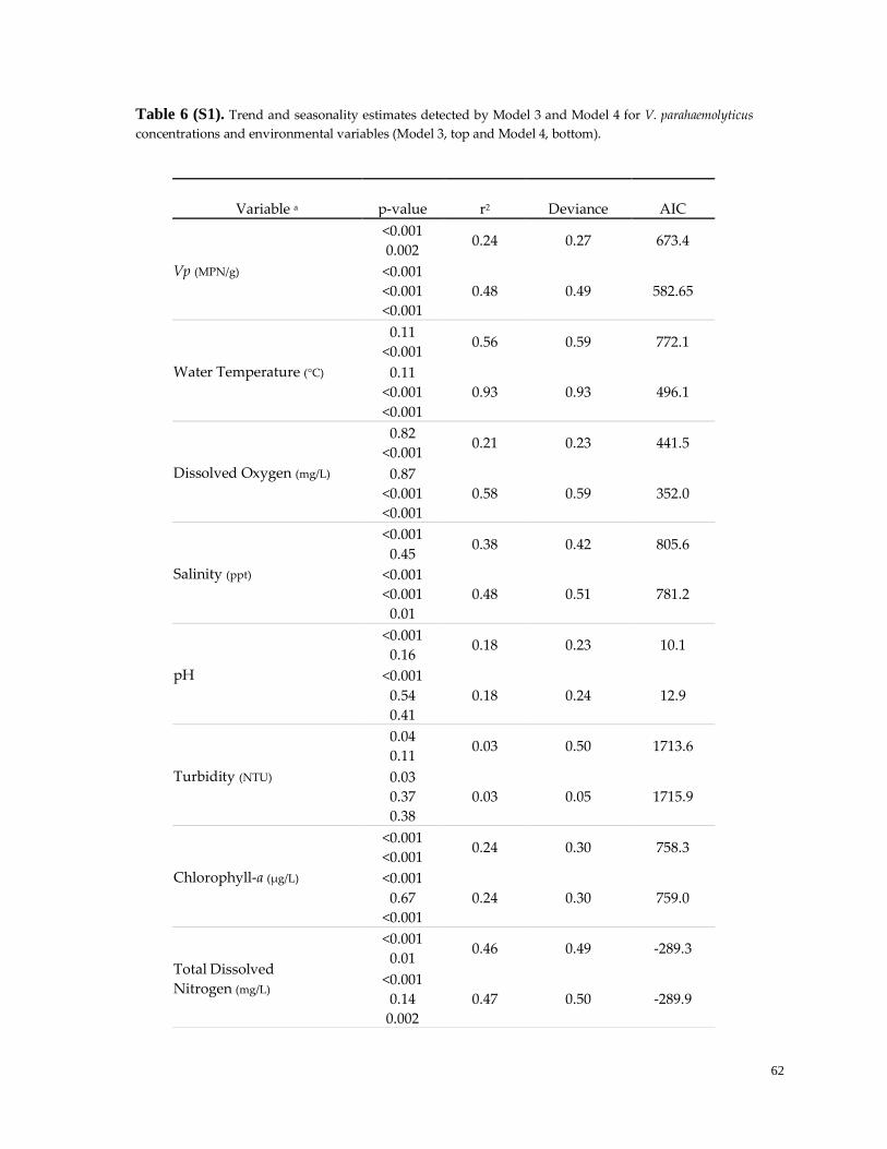
62

Table 6 (S1). Trend and seasonality estimates detected by Model 3 and Model 4 for V. parahaemolyticus

concentrations and environmental variables (Model 3, top and Model 4, bottom).

Variable a p-value r2 Deviance AIC

Vp (MPN/g)

<0.001

0.002 0.24 0.27 673.4

<0.001

<0.001

<0.001

0.48 0.49 582.65

Water Temperature (°C)

0.11

<0.001 0.56 0.59 772.1

0.11

<0.001

<0.001

0.93 0.93 496.1

Dissolved Oxygen (mg/L)

0.82

<0.001 0.21 0.23 441.5

0.87

<0.001

<0.001

0.58 0.59 352.0

Salinity (ppt)

<0.001

0.45 0.38 0.42 805.6

<0.001

<0.001

0.01

0.48 0.51 781.2

pH

<0.001

0.16 0.18 0.23 10.1

<0.001

0.54

0.41

0.18 0.24 12.9

Turbidity (NTU)

0.04

0.11 0.03 0.50 1713.6

0.03

0.37

0.38

0.03 0.05 1715.9

Chlorophyll-a (µg/L)

<0.001

<0.001 0.24 0.30 758.3

<0.001

0.67

<0.001

0.24 0.30 759.0

Total Dissolved

Nitrogen (mg/L)

<0.001

0.01 0.46 0.49 -289.3

<0.001

0.14

0.002

0.47 0.50 -289.9

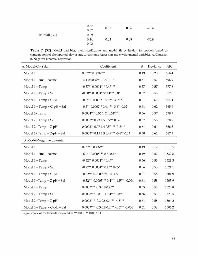
63

Table 7 (S2). Model variables, their significance and model fit evaluation for models based on

combinations of photoperiod, day of study, harmonic regression and environmental variables. A. Gaussian.

B. Negative binomial regression.

A. Model-Gaussian Coefficient r2 Deviance AIC

Model 1 0.57*** 0.0002*** 0.19 0.20 666.4

Model 1 + sine + cosine -4.1 0.0006*** -0.53 -1.6 0.51 0.52 596.9

Model 1 + Temp -0.37** 0.0004*** 0.47*** 0.57 0.57 577.6

Model 1 + Temp + Sal -0.30** 0.0004** 0.44*** 0.06 0.57 0.58 577.0

Model 1 + Temp + C-pH -0.3** 0.0003** 0.46*** -3.8*** 0.61 0.61 564.4

Model 1 + Temp + C-pH + Sal -0.3** 0.0002** 0.44*** -3.6** 0.02 0.61 0.62 565.9

Model 2+ Temp 0.0004*** 0.06 1.51 0.51*** 0.56 0.57 579.7

Model 2 + Temp + Sal 0.0003** 0.23 1.5 0.5*** 0.06 0.57 0.58 578.9

Model 2 +Temp + C-pH 0.0003** 0.07 1.4 0.50*** -3.8*** 0.61 0.61 566.3

Model 2+ Temp + C-pH + Sal 0.0003** 0.15 1.5 0.49*** -3.6** 0.03 0.60 0.62 567.7

B. Model-Negative binomial

Model 1 0.6*** 0.0006*** 0.19 0.17 1619.5

Model 1 + sine + cosine -6.2** 0.0005*** 0.6 -0.3*** 0.49 0.52 1532.8

Model 1 + Temp -0.32** 0.0004*** 0.4*** 0.56 0.53 1521.3

Model 1 + Temp + Sal -0.27** 0.0004** 0.4*** 0.05* 0.56 0.53 1521.1

Model 1 + Temp + C-pH -0.32*** 0.0003***; 0.4 -4.5 0.61 0.58 1501.9

Model 1 +Temp + C-pH + Sal -0.32*** 0.0003*** 0.4*** -4.5*** -0.004 0.61 0.58 1503.9

Model 2 + Temp 0.0003*** -0.3 0.8 0.4*** 0.55 0.52 1523.8

Model 2 + Temp + Sal 0.0003*** 0.03 1.1 0.4*** 0.05* 0.56 0.53 1523.5

Model 2 +Temp + C-pH 0.0003*** -0.3 0.8 0.4*** -4.5*** 0.61 0.58 1504.2

Model 2 + Temp + C-pH + Sal 0.0003*** -0.3 0.8 0.4*** -4.6*** -0.006 0.61 0.58 1506.2

significance of coefficients indicated as *** 0.001, ** 0.01, * 0.1

Rainfall (mm)

0.37

0.07 0.03 0.06 -76.4

0.29

0.24

0.02

0.04 0.08 -76.9

64

Chapter 2

The Seasonal Ecology of Vibrio parahaemolyticus and Plankton in a New Hampshire

Estuary

Meghan Hartwicka,b, Audrey Berensona,b, Cheryl A. Whistlera,b, Elena N. Naumovad, Stephen H. Jonesa,b,c

a Northeast Center for Vibrio Disease and Ecology, University of New Hampshire, Durham, NH b Department of Molecular, Cellular, and Biomedical Sciences, University of New Hampshire, Durham, NH c Department of Natural Resources and the Environment, University of New Hampshire, Durham, NH d Division of Nutrition Data Sciences, Friedman School of Nutrition Science and Policy, Tufts University,

Boston, MA; [email protected]

ABSTRACT

The emergence and establishment of Vibrio parahaemolyticus as a causative agent of shellfish-

borne illnesses in the Northeast United States has stimulated keen interest in understanding the

environmental conditions that may coincide with V. parahaemolyticus-associated-human health

risk in this region. Seasonal water temperature is an important characteristic of V.

parahaemolyticus dynamics and water temperature is used to manage shellfish harvesting-

related health risks in this region. However, a wide range of environmental variables including

copepods and chitinous phytoplankton in the water column, have also been reported as factors

that affect V. parahaemolyticus dynamics, though little is known regarding their significance in

the Northeast US. A holistic evaluation of the seasonal ecology of V. parahaemolyticus

concentration was conducted using three years of plankton community analysis, data for

nutrients, water quality and V. parahaemolyticus concentrations in water, sediment, and plankton

from a site in the Great Bay estuary (GBE) to identify the environmental variables that may

relate to V. parahaemolyticus dynamics in oysters. V. parahaemolyticus concentrations in sediment

and phytoplankton, Helicotheca tamensis, Rhizosolenia spp., water temperature, salinity and PO4

were identified as the optimal combination of variables to estimate the overall seasonality of V.

parahaemolyticus concentration in oysters. Together, this provides the first comprehensive report

of the microbial seasonal ecology of the GBE as it relates to plankton dynamics and V.

parahaemolyticus concentrations in oysters. The results of this work can be applied to monitoring

and mechanistic studies to improve our understanding of the seasonal dynamics that contribute

to pre-harvest risk for V. parahaemolyticus disease in this region.

INTRODUCTION

The emergence and establishment of Vibrio parahaemolyticus as a causative agent of shellfish-borne

illnesses in the Northeast United States has stimulated keen interest in understanding the

environmental conditions that may pose a human health risk in this region. The ecology of V.

parahaemolyticus has been the focus of numerous intensive studies and a wide array of

65

environmental variables associate with V. parahaemolyticus dynamics including water

temperature, salinity, pH, inorganic and organic nutrients, suspended solids-turbidity,

chlorophyll-a, light availability and meteorological conditions (Hartwick et al., 2019; Lovell, 2017;

Urquhart et al., 2016; Turner et al., 2014; Martinez-Urtaza et al., 2012; Vezzulli et al., 2009, Jones

and Summer-Brason, 1998, DePaola et al., 1990, Kaneko and Colwell, 1973). V. parahaemolyticus

can be associated with shellfish, sediment, micro and macroplankton, crabs and protozoa.

Though the majority of these associations are believed to be benign, abscesses and lesions

attributed to V. parahaemolyticus disease are also documented in corals, dolphins, sea otters, finfish

and shrimp (Erken et al., 2015, Vezzulli et al., 2013, Hughes et al., 2013; Martinez-Urtaza et al.,

2008).

Sediments provide nutrients and protection from environmental stressors for Vibrio

parahaemolyticus, especially during fall, winter and spring in cold and temperate water regions

(Alipour et al., 2014; Vezzulli et al., 2009; Venkateswaran et al., 1990; Kaneko and Colwell, 1973).

The water column is a common detection point for V. parahaemolyticus, though it is frequently the

organically-enriched particulate fractions of the water column, including marine snow, detritus

and suspended sediment, that are the point of interest for these studies (Williams et al., 2014;

Froelich et al., 2013). This is based on findings that suggest that V. parahaemolyticus prefers an

attachment versus free-living lifestyle and therefore more likely associates with these particles

(Parveen et al., 2008; Vezzulli et al., 2009; Johnson et al., 2013).

Whether shellfish are a preferred environment for Vibrio parahaemolyticus remains unclear,

however because of their commercial importance, the shellfish-V. parahaemolyticus relationship is

the most studied interaction. (Lovell et al., 2017; DePaola et al. 1990, 2003; Zimmerman et al. 2007).

Filter feeding of suspended material is the most likely route by which V. parahaemolyticus becomes

concentrated in shellfish (e.g., Froelich et al. 2013). Kaneko and Colwell (1977) first described how

this filter feeding likely contributes to the accumulation of V. parahaemolyticus in the Chesapeake

Bay as a seasonal cycle between sediment, water, plankton and shellfish. Given this, copepods

and chitinous phytoplankton or water quality variables, such as organic and inorganic nutrients

and chlorophyll-a that have often been associated with phytoplankton abundance (Caburlotto et

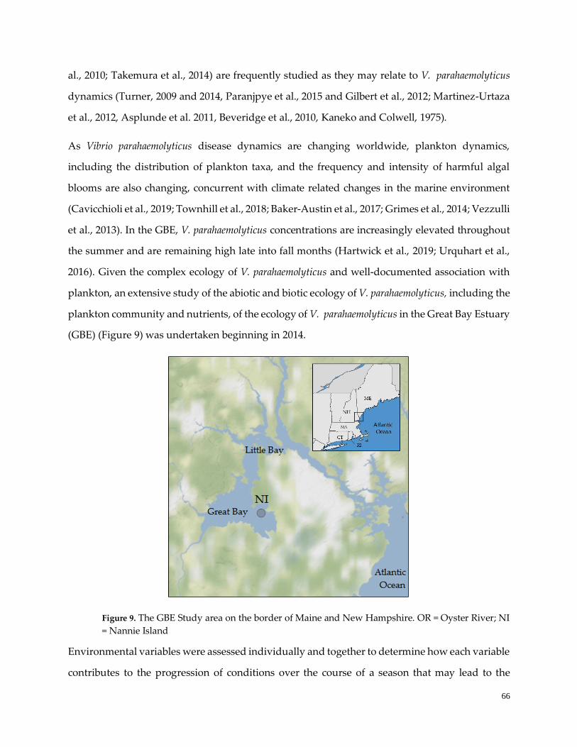
66

al., 2010; Takemura et al., 2014) are frequently studied as they may relate to V. parahaemolyticus

dynamics (Turner, 2009 and 2014, Paranjpye et al., 2015 and Gilbert et al., 2012; Martinez-Urtaza

et al., 2012, Asplunde et al. 2011, Beveridge et al., 2010, Kaneko and Colwell, 1975).

As Vibrio parahaemolyticus disease dynamics are changing worldwide, plankton dynamics,

including the distribution of plankton taxa, and the frequency and intensity of harmful algal

blooms are also changing, concurrent with climate related changes in the marine environment

(Cavicchioli et al., 2019; Townhill et al., 2018; Baker-Austin et al., 2017; Grimes et al., 2014; Vezzulli

et al., 2013). In the GBE, V. parahaemolyticus concentrations are increasingly elevated throughout

the summer and are remaining high late into fall months (Hartwick et al., 2019; Urquhart et al.,

2016). Given the complex ecology of V. parahaemolyticus and well-documented association with

plankton, an extensive study of the abiotic and biotic ecology of V. parahaemolyticus, including the

plankton community and nutrients, of the ecology of V. parahaemolyticus in the Great Bay Estuary

(GBE) (Figure 9) was undertaken beginning in 2014.

Figure 9. The GBE Study area on the border of Maine and New Hampshire. OR = Oyster River; NI

= Nannie Island

Environmental variables were assessed individually and together to determine how each variable

contributes to the progression of conditions over the course of a season that may lead to the

67

accumulation of Vibrio parahaemolyticus in oysters and characterize the environmental factors that

may be driving the changing dynamics of V. parahaemolyticus in the GBE. This study represents

the first comprehensive, multi-year assessment of the seasonal microbial ecology of V.

parahaemolyticus concentrations in the GBE. The outcomes of this work contribute to a better

understanding of the conditions that may contribute to V. parahaemolyticus dynamics in the

Northeast, US and identifies new targets for monitoring and mechanistic studies to understand

human health risks.

METHODS

Study sites, environmental sampling and bacterial analysis

The study area was the Great Bay estuary of New Hampshire, focused at a site near Nannie

Island (NI) that has a significant oyster (Crassostrea virginica) bed and is a long-term monitoring

location (Urquhart et al. 2016; Jones and Summer-Brason 1998). The estuary has been monitored

for over 30 consecutive years (March-December) by multiple agencies, including the Great Bay

National Estuarine Research Reserve (GBNERR) and their System Wide Monitoring Program

(SWMP). Continuous (Q15) water temperature, salinity, dissolved oxygen (DO), pH, and

turbidity data were obtained from SWMP from 2014-2016 for times simultaneous with and

preceding sampling events. Nutrient and related parameter data for grab samples; Non-

Purgeable Organic Carbon (NPOC), Total Dissolved Nitrogen (TDN), Nitrate and Nitrite (NO3 +

NO2,) Ammonium (NH4), Orthophosphate (PO4), Dissolved Organic Nitrogen (DON), Total

Suspended Solids (TSS), Particulate Carbon (PC), Particulate Nitrogen (PN), chlorophyll-a (CHL)

and pheophytin (PHEO) measurements were obtained from the SWMP database

(https://cdmo.baruch.sc.edu/dges/).

Oyster, sediment, water and plankton samples, referred to as matrices for Vibrio parahaemolyticus,

were collected concurrently with time of sample water temperature, salinity, pH and dissolved

oxygen (DO) measurements using YSI 6600 and EXO multiprobe sondes (Yellow Springs

Instruments, Yellow Springs, Ohio), during low tide from the NI study site. Plankton samples

were collected using a 53 µm mesh net (Aquatic Instruments). Sediment, oyster, phyto- and

zooplankton samples were processed and analyzed for Vibrio detection according to previously

68

published methods with alkaline peptone water enrichment, Vibrio CHROMAgar and the FDA

established PCR (Hartwick et al. 2019) and MPN calculations at Jackson Estuarine Lab (JEL).

Probable Vibrio isolates were confirmed as V. parahaemolyticus by PCR detection of the tlh gene

(Urquhart et al., 2016, Hartwick et al., 2019, Kaysner and DePaola (BAM), 2004).

Plankton collection and phototactic separation

Plankton samples were collected in duplicate using a 53 µm mesh net and three different methods

for collecting adequate and increasingly more accurate volumes of water: in 2014 a Student Net

(Aquatic Instruments, Florida USA), was used during ten weighted tows to collect ~140L of water;

for March 2015 through Oct 2015 a Niskin sampler with Student Net (Aquatic Instruments,

Florida USA) was used to collect 160L; and for October 2015 through December 2016 a 30L

Schindler Patalas (Wildco, Florida, USA) was used to collect 180L. One sub-sample was

phototactically separated to provide efficient separation of the phytoplankton from the

zooplankton fractions using a method and device for plankton separation (Leland and Haney,

2018). Time series trials were performed in triplicate at 0, 10, 20, 30, 40 minutes with optimum

separation efficiency being observed at 40 minutes. This separation time was in agreement with

previous observations (Nancy Leland pers. comm). Sample one, separated into phyto- and

zooplankton fractions was filtered in 53 um pore size hand-prepared filter cones using Nitex

Bolting Cloth (Wildco, Florida, USA), concentrated and weighed. Zoo and phytoplankton

samples were processed identically to oyster, water and sediment samples accordingly to

previously published methods (Urquhart et al., 2016, Hartwick et al., 2019, Kaysner and DePaola,

2004) to determine Vibrio parahaemolyticus MPN/g. The subsample was then resuspended to a

volume of 50 mL in <53 µm filtrate water from NI and preserved with 1% sucrose formalin (US

EPA, 2003) for sample community identification, enumeration and biomass concentration

(cells/L) determination.

Plankton biomass and community analysis

Plankton community enumeration and concentration determinations were performed by

methods consistent with standard methods for plankton analysis (USEPA, 2003) using a phase-

contrast microscope and a 1mL grafted Sedgwick rafter (Wildco, Florida USA). Plankton

69

identification was confirmed with a combination of identification key resources including: Dolan

and Cooper, 2006 and Baker et al., 2012. Samples were analyzed with a phase-contrast microscope

at 400x magnification (Olympus, USA) to count 10 non-consecutive columns (100 cells total).

Sample dilution was conducted when necessary, for samples too abundant for accurate counting

using deionized (DI) water. Counts were transformed to cells/L for each taxa observed in the

sample

Statistical analysis

All statistical computations were performed in the R Statistical Program and Environment,

version 3.5.3 (R Core Team, 2019) and vegan: Community Ecology Package, 2.5-2 (Oksanen et al.,

2018). Multiple steps of data analysis were performed to evaluate the relationship between

plankton, environmental determinants and V. parahaemolyticus concentrations in the GBE.

Significance for all analysis was determined by p < 0.05.

Environmental variables

MPN values for Vibrio parahaemolyticus concentrations were log-transformed for analysis to

approximate normality and reduce skewness. Total phytoplankton and zooplankton/L were

determined by subtracting the total number of nauplii, copepods and Tintinnida from the total

plankton abundance/L. The V. parahaemolyticus concentration associated with a gram wet weight

of phyto or zooplankton was transformed to V. parahaemolyticus concentration associated with

phyto or zooplankton/L by dividing the MPN by the number of L required to produce one gram

of phyto or zooplankton. Relative concentrations between matrices were compared by two-way

analysis of variance (ANOVA).

Plankton sample and community analysis

Total Abundance (TA) and Relative Abundance (RA), species richness, evenness and Shannon’s

H were calculated for the entire study period. Taxa observed in collected samples were assessed

as Abundant (> 4% of total), Common (≤ 4% and ≥ 0.1%) or Rare ( <0.1%) in the GBE plankton

community according to the DAFOR semi-quantitative abundance classification. Plankton counts

were log + 1 transformed to reduce skew and kurtosis. Rare taxa (abundance <0.1%) were not

70

included in community analysis or structural equation modeling. Seasonal community

assemblage was assessed between calendar seasons (spring: March to June 21st, summer: June

22nd through September 21st and fall: September 22nd to December, and years (2014, 2015 and

2016) by Permanova, Multi Response Permutation Procedure (MRPP), and Indicator Species

Analysis (ISA).

Seasonality

The seasonality and general trend in the environmental variables were explored with:

Model 1: 𝐸(𝑌𝑡) = 𝛽0 + 𝛽1𝑡 + 𝛽p𝑃ℎ𝑜𝑡𝑜𝑝𝑒𝑟𝑖𝑜𝑑, and (1)

Model 2: 𝐸(𝑌𝑡) = 𝛽0 + 𝛽1𝑡 + 𝛽𝑠 sin(2𝜋𝜔𝑡) + 𝛽𝑐 cos(2𝜋𝜔𝑡). (2)

to fit periodicity and trends of the seasonal oscillations (Hartwick et al., 2019). In both models, 𝑌𝑡

is the daily time series for the outcome of interest, 𝛽0 is the intercept, t is the daily time series,

𝛽1indicated a general trend in the variable of interest. Model 1 contains the photoperiod variable

𝛽p𝑃ℎ𝑜𝑡𝑜𝑝𝑒𝑟𝑖𝑜𝑑 and Model 2 uses harmonic regression terms for the calendar day in the study

where 𝛽𝑠 and 𝛽𝑐 are the coefficients of the harmonic terms and ω is the term representing the

annual cycle (365.25 days, ω=1/365.25). The peak timing of the periodic oscillations identified by

Model 2 was determined by calculating the phase shift:

𝜓 = arctan (𝑠

𝑐) + 𝑘. (3)

When 𝑆 and 𝑐 were positive, 𝑘 = 0. When 𝑆 < 0 and 𝑐 > 0, 𝑘 = 2𝜋 and when 𝑆 and 𝑐 were

negative, or when 𝑆 > 0 and 𝑐 < 0, then 𝑘 = 𝜋. The phase shift (𝜓) was then multiplied by

365.25. Confidence intervals (CI) of the peak timing were calculated by determining the estimated

variance of the phase shift (𝜓) where (𝜎𝛽𝑐𝛽𝑠) is the covariance and 𝑠

2 and 𝑐2 are the variances of

𝛽𝑠 and 𝛽𝑐 in the following equation:

𝑣𝑎𝑟(𝜓) = (𝜎𝛽𝑠𝛽𝑐)

2+ (𝜎𝛽𝑐𝛽𝑠)

2−(2𝜎𝛽𝑐𝛽𝑠 𝛽𝑠𝛽𝑐)

(𝑠2+ 𝑐

2)(𝑠2+ 𝑐

2)2 . (4)

CI values for the peak timing estimates were determined as: 1.96 ∗ √𝑉𝑎𝑟(𝜓) ∗ 365.25/2𝜋. The

seasonality of the environmental variables was evaluated by the significance of the coefficients,

71

the deviance explained, AIC, and coefficient of determination (r2) value of Model 1 and 2

(Naumova et al., 2007, Alarcon Falconi et al., 2018).

Correlation

The Mantel test and Spearman rank correlation analysis were performed for Vibrio

parahaemolyticus concentrations in all matrices, water quality, dissolved nutrients and plankton

community data to assess the relationship of environmental variables to V. parahaemolyticus

dynamics in oysters.

Systems ecology modeling

Partial Least Squared Residual models (PLSR) were used to identify the most significant seasonal

variables associated with Vibrio parahaemolyticus concentration in oysters based on a variable

importance score (VIP) >0.8. PLSR model performance was evaluated by Residual Mean Square

Error (RMSE) and deviance explained. The variables identified by PLSR were integrated into

structural equation models (SEM) to evaluated and explore potential drivers of the seasonal

accumulation of V. parahaemolyticus in oysters in the GBE. A correlation table was provided to

illustrate the correlation matrix of the environmental variables of interest. SEM model fit was

evaluated based on the relationships between environmental variables as they were hypothesized

by the SEM model and then compared to the actual environmental variable relationships that

were observed in the correlation matrix. Chi-square (χ2) > 0.05 indicates that there is no

significant difference between the observed correlation matrix and specified variable

relationships in the SEM and therefore is a good representation of the relationships of the

environmental variables. SEM model fit where χ2 p > 0.05 were then evaluated by model

likelihood (H1 compared to H0), Comparative Fit (>= 0.90) Tucker Lewis Fit (>= 0.95), Standardized

Root Mean Square Residual (SRMR < 0.08) AIC, and the coefficient of determination (r2).

RESULTS

Vibrio parahaemolyticus, total plankton and environmental variable detection and timing

Water and other ecosystem matrices were analyzed for water quality conditions, plankton

community abundance and Vibrio parahaemolyticus concentrations to understand the seasonal

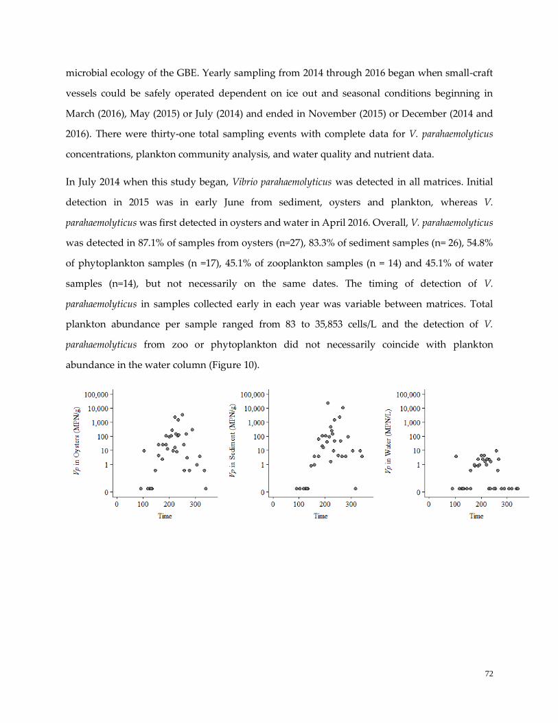
72

microbial ecology of the GBE. Yearly sampling from 2014 through 2016 began when small-craft

vessels could be safely operated dependent on ice out and seasonal conditions beginning in

March (2016), May (2015) or July (2014) and ended in November (2015) or December (2014 and

2016). There were thirty-one total sampling events with complete data for V. parahaemolyticus

concentrations, plankton community analysis, and water quality and nutrient data.

In July 2014 when this study began, Vibrio parahaemolyticus was detected in all matrices. Initial

detection in 2015 was in early June from sediment, oysters and plankton, whereas V.

parahaemolyticus was first detected in oysters and water in April 2016. Overall, V. parahaemolyticus

was detected in 87.1% of samples from oysters (n=27), 83.3% of sediment samples (n= 26), 54.8%

of phytoplankton samples (n =17), 45.1% of zooplankton samples (n = 14) and 45.1% of water

samples (n=14), but not necessarily on the same dates. The timing of detection of V.

parahaemolyticus in samples collected early in each year was variable between matrices. Total

plankton abundance per sample ranged from 83 to 35,853 cells/L and the detection of V.

parahaemolyticus from zoo or phytoplankton did not necessarily coincide with plankton

abundance in the water column (Figure 10).

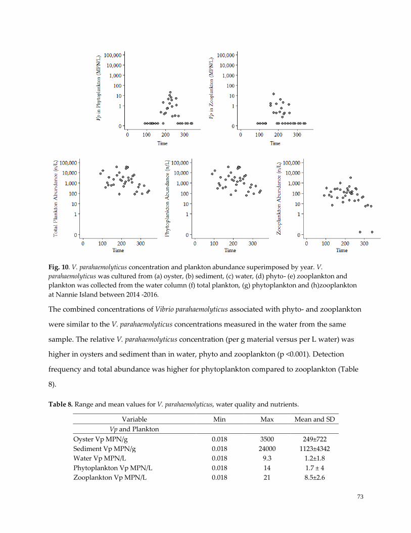
73

Fig. 10. V. parahaemolyticus concentration and plankton abundance superimposed by year. V.

parahaemolyticus was cultured from (a) oyster, (b) sediment, (c) water, (d) phyto- (e) zooplankton and

plankton was collected from the water column (f) total plankton, (g) phytoplankton and (h)zooplankton

at Nannie Island between 2014 -2016.

The combined concentrations of Vibrio parahaemolyticus associated with phyto- and zooplankton

were similar to the V. parahaemolyticus concentrations measured in the water from the same

sample. The relative V. parahaemolyticus concentration (per g material versus per L water) was

higher in oysters and sediment than in water, phyto and zooplankton (p <0.001). Detection

frequency and total abundance was higher for phytoplankton compared to zooplankton (Table

8).

Table 8. Range and mean values for V. parahaemolyticus, water quality and nutrients.

Variable Min Max Mean and SD

Vp and Plankton

Oyster Vp MPN/g 0.018 3500 249±722

Sediment Vp MPN/g 0.018 24000 1123±4342

Water Vp MPN/L 0.018 9.3 1.2±1.8

Phytoplankton Vp MPN/L 0.018 14 1.7 ± 4

Zooplankton Vp MPN/L 0.018 21 8.5±2.6

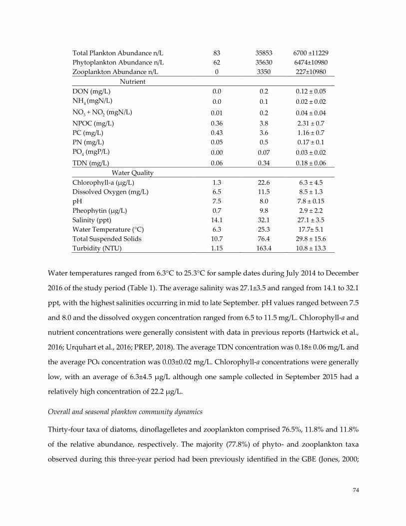
74

Total Plankton Abundance n/L 83 35853 6700 ±11229

Phytoplankton Abundance n/L 62 35630 6474±10980

Zooplankton Abundance n/L 0 3350 227±10980

Nutrient

DON (mg/L) 0.0 0.2 0.12 ± 0.05

NH4 (mgN/L) 0.0 0.1 0.02 ± 0.02

NO3 + NO

2 (mgN/L) 0.01 0.2 0.04 ± 0.04

NPOC (mg/L) 0.36 3.8 2.31 ± 0.7

PC (mg/L) 0.43 3.6 1.16 ± 0.7

PN (mg/L) 0.05 0.5 0.17 ± 0.1

PO4 (mgP/L) 0.00 0.07 0.03 ± 0.02

TDN (mg/L) 0.06 0.34 0.18 ± 0.06

Water Quality

Chlorophyll-a (µg/L) 1.3 22.6 6.3 ± 4.5

Dissolved Oxygen (mg/L) 6.5 11.5 8.5 ± 1.3

pH 7.5 8.0 7.8 ± 0.15

Pheophytin (µg/L) 0.7 9.8 2.9 ± 2.2

Salinity (ppt) 14.1 32.1 27.1 ± 3.5

Water Temperature (°C) 6.3 25.3 17.7± 5.1

Total Suspended Solids 10.7 76.4 29.8 ± 15.6

Turbidity (NTU) 1.15 163.4 10.8 ± 13.3

Water temperatures ranged from 6.3°C to 25.3°C for sample dates during July 2014 to December

2016 of the study period (Table 1). The average salinity was 27.1±3.5 and ranged from 14.1 to 32.1

ppt, with the highest salinities occurring in mid to late September. pH values ranged between 7.5

and 8.0 and the dissolved oxygen concentration ranged from 6.5 to 11.5 mg/L. Chlorophyll-a and

nutrient concentrations were generally consistent with data in previous reports (Hartwick et al.,

2016; Urquhart et al., 2016; PREP, 2018). The average TDN concentration was 0.18± 0.06 mg/L and

the average PO4 concentration was 0.03±0.02 mg/L. Chlorophyll-a concentrations were generally

low, with an average of 6.3±4.5 µg/L although one sample collected in September 2015 had a

relatively high concentration of 22.2 µg/L.

Overall and seasonal plankton community dynamics

Thirty-four taxa of diatoms, dinoflagelletes and zooplankton comprised 76.5%, 11.8% and 11.8%

of the relative abundance, respectively. The majority (77.8%) of phyto- and zooplankton taxa

observed during this three-year period had been previously identified in the GBE (Jones, 2000;

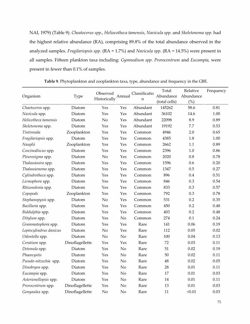
75

NAI, 1979) (Table 9). Cheatocerus spp., Heliocotheca tamensis, Navicula spp. and Skeletonema spp. had

the highest relative abundance (RA), comprising 89.8% of the total abundance observed in the

analyzed samples. Fragilariopsis spp. (RA = 1.7%) and Navicula spp. (RA = 14.5%) were present in

all samples. Fifteen plankton taxa including: Gymnodium spp. Prorocentrum and Eucampia, were

present in fewer than 0.1% of samples.

Table 9. Phytoplankton and zooplankton taxa, type, abundance and frequency in the GBE.

Organism Type Observed

Historically Annual

Classificatio

n

Total

Abundance

(total cells)

Relative

Abundance

(%)

Frequency

Chaetoceros spp. Diatom Yes Yes Abundant 145262 58.6 0.81

Navicula spp. Diatom Yes Yes Abundant 36102 14.6 1.00

Helicotheca tamensis Diatom No Yes Abundant 22098 8.9 0.89

Skeletonema spp. Diatom Yes Yes Abundant 19192 7.7 0.53

Tintinnida Zooplankton Yes Yes Common 4946 2.0 0.65

Fragilariopsis spp. Diatom Yes Yes Common 4385 1.8 1.00

Nauplii Zooplankton Yes Yes Common 2662 1.1 0.89

Coscinodiscus spp. Diatom Yes Yes Common 2396 1.0 0.86

Pleurosigma spp. Diatom No Yes Common 2020 0.8 0.78

Thalassiosira spp. Diatom Yes Yes Common 1596 0.6 0.20

Thalassionema spp. Diatom Yes Yes Common 1347 0.5 0.27

Cylindrotheca spp. Diatom Yes Yes Common 896 0.4 0.51

Licmophora spp. Diatom Yes Yes Common 846 0.3 0.54

Rhizosolenia spp. Diatom Yes Yes Common 833 0.3 0.57

Copepods Zooplankton Yes Yes Common 792 0.3 0.78

Stephanopyxis spp. Diatom No Yes Common 531 0.2 0.35

Bacillaria spp. Diatom Yes Yes Common 450 0.2 0.48

Biddulphia spp. Diatom Yes Yes Common 403 0.2 0.48

Ditylum spp. Diatom Yes No Common 274 0.1 0.24

Grammatophora spp. Diatom Yes Yes Rare 141 0.06 0.19

Leptocylindrus danicus Diatom No Yes Rare 112 0.05 0.02

Odontella spp. Diatom No No Rare 100 0.04 0.13

Ceratium spp. Dinoflagellette Yes Yes Rare 72 0.03 0.11

Detonula spp. Diatom Yes No Rare 51 0.02 0.19

Phaeocystis Diatom Yes No Rare 50 0.02 0.11

Pseudo-nitzschia spp. Diatom Yes No Rare 48 0.02 0.05

Dinobryon spp. Diatom Yes No Rare 28 0.01 0.11

Eucampia spp. Diatom Yes No Rare 17 0.01 0.03

Asterionellopsis spp. Diatom Yes No Rare 14 0.01 0.11

Prorocentrum spp. Dinoflagellette Yes No Rare 13 0.01 0.03

Gonyaulax spp. Dinoflagellette No No Rare 11 <0.01 0.03

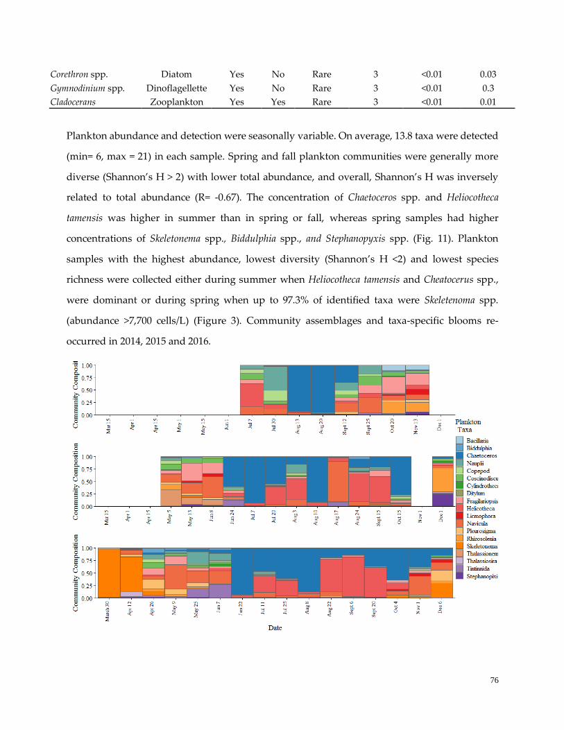
76

Corethron spp. Diatom Yes No Rare 3 <0.01 0.03

Gymnodinium spp. Dinoflagellette Yes No Rare 3 <0.01 0.3

Cladocerans Zooplankton Yes Yes Rare 3 <0.01 0.01

Plankton abundance and detection were seasonally variable. On average, 13.8 taxa were detected

(min= 6, max = 21) in each sample. Spring and fall plankton communities were generally more

diverse (Shannon’s H > 2) with lower total abundance, and overall, Shannon’s H was inversely

related to total abundance (R= -0.67). The concentration of Chaetoceros spp. and Heliocotheca

tamensis was higher in summer than in spring or fall, whereas spring samples had higher

concentrations of Skeletonema spp., Biddulphia spp., and Stephanopyxis spp. (Fig. 11). Plankton

samples with the highest abundance, lowest diversity (Shannon’s H <2) and lowest species

richness were collected either during summer when Heliocotheca tamensis and Cheatocerus spp.,

were dominant or during spring when up to 97.3% of identified taxa were Skeletenoma spp.

(abundance >7,700 cells/L) (Figure 3). Community assemblages and taxa-specific blooms re-

occurred in 2014, 2015 and 2016.

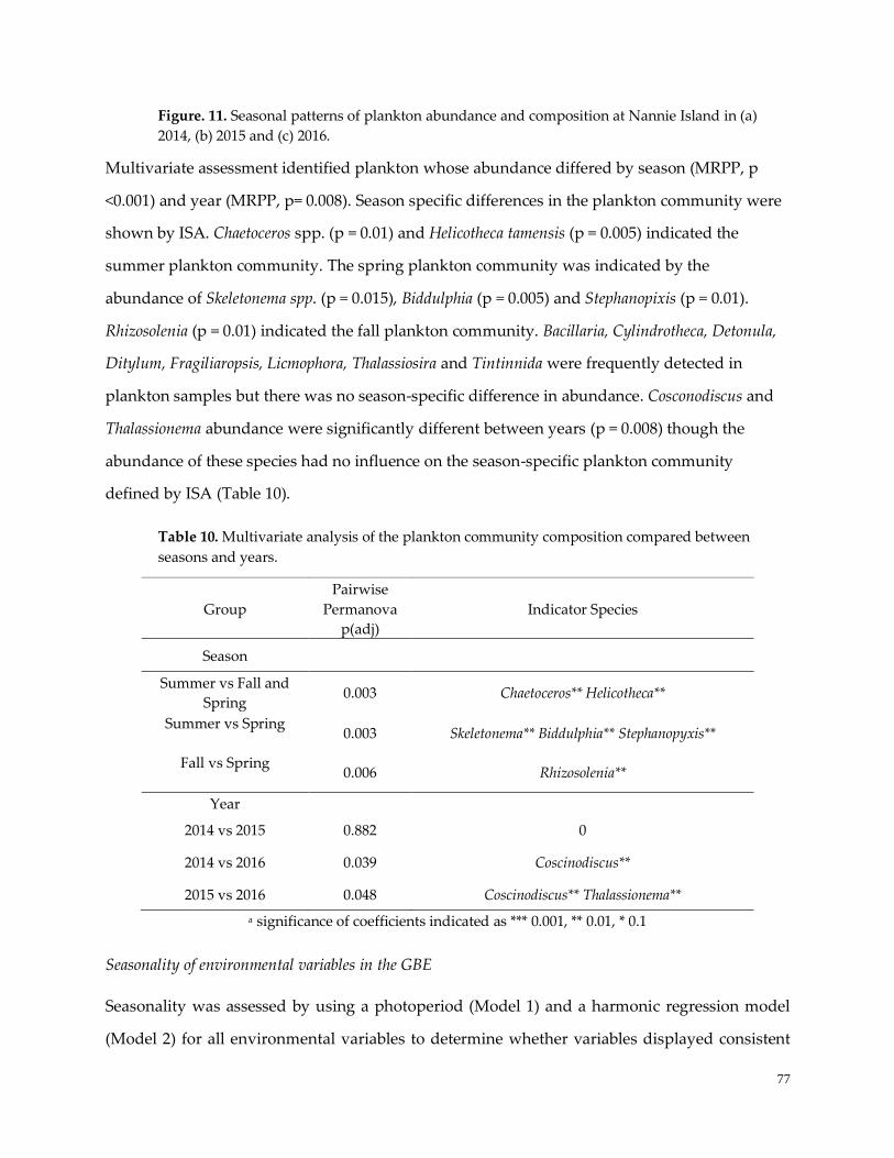
77

Figure. 11. Seasonal patterns of plankton abundance and composition at Nannie Island in (a)

2014, (b) 2015 and (c) 2016.

Multivariate assessment identified plankton whose abundance differed by season (MRPP, p

<0.001) and year (MRPP, p= 0.008). Season specific differences in the plankton community were

shown by ISA. Chaetoceros spp. (p = 0.01) and Helicotheca tamensis (p = 0.005) indicated the

summer plankton community. The spring plankton community was indicated by the

abundance of Skeletonema spp. (p = 0.015), Biddulphia (p = 0.005) and Stephanopixis (p = 0.01).

Rhizosolenia (p = 0.01) indicated the fall plankton community. Bacillaria, Cylindrotheca, Detonula,

Ditylum, Fragiliaropsis, Licmophora, Thalassiosira and Tintinnida were frequently detected in

plankton samples but there was no season-specific difference in abundance. Cosconodiscus and

Thalassionema abundance were significantly different between years (p = 0.008) though the

abundance of these species had no influence on the season-specific plankton community

defined by ISA (Table 10).

Table 10. Multivariate analysis of the plankton community composition compared between

seasons and years.

Group

Pairwise

Permanova

p(adj)

Indicator Species

Season

Summer vs Fall and

Spring 0.003 Chaetoceros** Helicotheca**

Summer vs Spring

0.003 Skeletonema** Biddulphia** Stephanopyxis**

Fall vs Spring

0.006 Rhizosolenia**

Year

2014 vs 2015 0.882 0

2014 vs 2016 0.039 Coscinodiscus**

2015 vs 2016 0.048 Coscinodiscus** Thalassionema**

a significance of coefficients indicated as *** 0.001, ** 0.01, * 0.1

Seasonality of environmental variables in the GBE

Seasonality was assessed by using a photoperiod (Model 1) and a harmonic regression model

(Model 2) for all environmental variables to determine whether variables displayed consistent

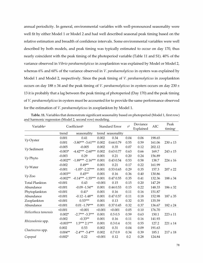
78

annual periodicity. In general, environmental variables with well-pronounced seasonality were

well fit by either Model 1 or Model 2 and had well described seasonal peak timing based on the

relative estimation and breadth of confidence intervals. Some environmental variables were well

described by both models, and peak timing was typically estimated to occur on day 170, thus

nearly coincident with the peak timing of the photoperiod variable (Table 11 and S1). 40% of the

variance observed in Vibrio parahaemolyticus in zooplankton was explained by Model or Model 2,

whereas 6% and 60% of the variance observed in V. parahaemolyticus in oysters was explained by

Model 1 and Model 2, respectively. Since the peak timing of V. parahaemolyticus in zooplankton

occurs on day 188 ± 34 and the peak timing of V. parahaemolyticus in oysters occurs on day 230 ±

13 it is probably that a lag between the peak timing of photoperiod (Day 170) and the peak timing

of V. parahaemolyticus in oysters must be accounted for to provide the same performance observed

for the estimation of V. parahaemolyticus in zooplankton by Model 1.

Table. 11. Variables that demonstrate significant seasonality based on photoperiod (Model 1, first row)

and harmonic regression (Model 2, second row) modeling.

Variablea Coefficientb Standard Error r2 Deviance

Explained AIC

Peak

timingc

trend seasonality trend seasonality

Vp Oyster 0.001 0.41 0.002 0.34 0.04 0.06 198.65

0.001 -3.80*** -3.61*** 0.002 0.64 0.79 0.55 0.59 161.06 230 ± 13

Vp Sediment -0.005 -0.005 0.002 0.35 0.07 0.12 202.12

-0.003* -4.42*** -2.60*** 0.002 0.63 0.77 0.63 0.66 169.7 243 ± 15

Vp Phyto -0.003 0.29 0.001 0.21 0.20 0.24 156.89

-0.002** -1.89*** -2.16*** 0.001 0.43 0.54 0.53 0.58 138.7 224 ± 16

Vp Water -0.002 0.49** 0.001 0.21 0.17 0.22 161.99

-0.001 -1.05* -2.27*** 0.001 0.53 0.65 0.29 0.35 157.3 207 ± 22

Vp Zoo -0.003** 0.45** 0.001 0.16 0.36 0.40 130.86

-0.002** -0.14*** -1.55*** 0.001 0.47 0.55 0.35 0.41 132.36 188 ± 34

Total Plankton

Abundance

<0.001 0.43 <0.001 0.15 0.15 0.20 147.29

<0.001 -0.09 -1.54** 0.001 0.44 0.53 0.15 0.22 148.33 186 ± 32

Phytoplankton

Abundance

<0.001 0.41* 0.001 0.16 0.11 0.16 151.87

<0.001 -0.12 -1.48** 0.001 0.47 0.57 0.11 0.18 152.98 187 ± 35

Zooplankton

Abundance

<0.001 0.53*** 0.001 0.13 0.32 0.35 135.59

<0.001 0.01 -1.79*** 0.001 0.37 0.45 0.32 0.37 136.67 182 ± 24

Helicotheca tamensis <0.001 <0.001 <0.001 <0.001 0.05 0.10 176.70

0.002* -2.7*** -3.3*** 0.001 0.5 0.5 0.59 0.63 150.1 223 ± 11

Rhizosolenia spp. -0.002 -0.33** 0.001 0.16 0.11 0.16 141.93

-0.003*** 1.5*** 2.1*** 0.001 0.3 0.4 0.51 0.55 127.2 221 ± 14

Chaetoceros spp. 0.002 0.53 0.002 0.31 0.04 0.09 191.63

0.004** -2.4*** -3.4*** 0.002 0.7 0.9 0.34 0.39 185.1 217 ± 18

Copepod -0.002* 0.22 <0.001 0.12 0.2 0.28 124.84

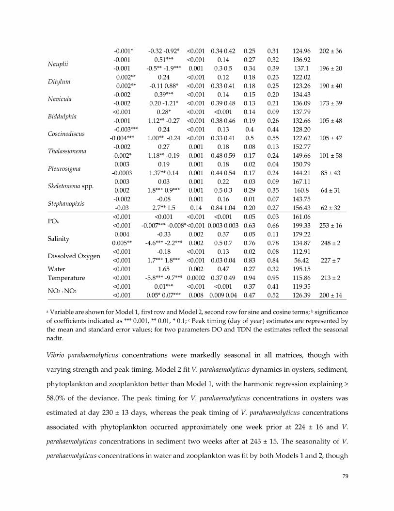
79

-0.001* -0.32 -0.92* <0.001 0.34 0.42 0.25 0.31 124.96 202 ± 36

Nauplii -0.001 0.51*** <0.001 0.14 0.27 0.32 136.92

-0.001 -0.5** -1.9*** 0.001 0.3 0.5 0.34 0.39 137.1 196 ± 20

Ditylum 0.002** 0.24 <0.001 0.12 0.18 0.23 122.02

0.002** -0.11 0.88* <0.001 0.33 0.41 0.18 0.25 123.26 190 ± 40

Navicula -0.002 0.39*** <0.001 0.14 0.15 0.20 134.43

-0.002 0.20 -1.21* <0.001 0.39 0.48 0.13 0.21 136.09 173 ± 39

Biddulphia <0.001 0.28* <0.001 <0.001 0.14 0.09 137.79

-0.001 1.12** -0.27 <0.001 0.38 0.46 0.19 0.26 132.66 105 ± 48

Coscinodiscus -0.003*** 0.24 <0.001 0.13 0.4 0.44 128.20

-0.004*** 1.00** -0.24 <0.001 0.33 0.41 0.5 0.55 122.62 105 ± 47

Thalassionema -0.002 0.27 0.001 0.18 0.08 0.13 152.77

-0.002* 1.18** -0.19 0.001 0.48 0.59 0.17 0.24 149.66 101 ± 58

Pleurosigma 0.003 0.19 0.001 0.18 0.02 0.04 150.79

-0.0003 1.37** 0.14 0.001 0.44 0.54 0.17 0.24 144.21 85 ± 43

Skeletonema spp. 0.003 0.03 0.001 0.22 0.03 0.09 167.11

0.002 1.8*** 0.9*** 0.001 0.5 0.3 0.29 0.35 160.8 64 ± 31

Stephanopixis -0.002 -0.08 0.001 0.16 0.01 0.07 143.75

-0.03 2.7** 1.5 0.14 0.84 1.04 0.20 0.27 156.43 62 ± 32

PO4 <0.001 <0.001 <0.001 <0.001 0.05 0.03 161.06

<0.001 -0.007*** -0.008* <0.001 0.003 0.003 0.63 0.66 199.33 253 ± 16

Salinity 0.004 -0.33 0.002 0.37 0.05 0.11 179.22

0.005** -4.6*** -2.2*** 0.002 0.5 0.7 0.76 0.78 134.87 248 ± 2

Dissolved Oxygen <0.001 -0.18 <0.001 0.13 0.02 0.08 112.91

<0.001 1.7*** 1.8*** <0.001 0.03 0.04 0.83 0.84 56.42 227 ± 7

Water

Temperature

<0.001 1.65 0.002 0.47 0.27 0.32 195.15

<0.001 -5.8*** -9.7*** 0.0002 0.37 0.49 0.94 0.95 115.86 213 ± 2

NO3 + NO2 <0.001 0.01*** <0.001 <0.001 0.37 0.41 119.35

<0.001 0.05* 0.07*** 0.008 0.009 0.04 0.47 0.52 126.39 200 ± 14

a Variable are shown for Model 1, first row and Model 2, second row for sine and cosine terms; b significance

of coefficients indicated as *** 0.001, ** 0.01, * 0.1; c Peak timing (day of year) estimates are represented by

the mean and standard error values; for two parameters DO and TDN the estimates reflect the seasonal

nadir.

Vibrio parahaemolyticus concentrations were markedly seasonal in all matrices, though with

varying strength and peak timing. Model 2 fit V. parahaemolyticus dynamics in oysters, sediment,

phytoplankton and zooplankton better than Model 1, with the harmonic regression explaining >

58.0% of the deviance. The peak timing for V. parahaemolyticus concentrations in oysters was

estimated at day 230 ± 13 days, whereas the peak timing of V. parahaemolyticus concentrations

associated with phytoplankton occurred approximately one week prior at 224 ± 16 and V.

parahaemolyticus concentrations in sediment two weeks after at 243 ± 15. The seasonality of V.

parahaemolyticus concentrations in water and zooplankton was fit by both Models 1 and 2, though

80

the strength of seasonality was less pronounced and the peak timing in these matrices occurred

at least three weeks prior to other matrices (days 207 ± 22 and 188 ± 34, respectively). The

seasonality of total plankton, phytoplankton and zooplankton abundances also varied, though

the peak timing estimates were similar (ranging from day 182 to 187). Models 1 and 2 both fit the

seasonality of zooplankton abundance well, while seasonality was less pronounced for total

plankton and phytoplankton abundance. Deviance explained by either model was >35% for

zooplankton abundance compared to < 22% deviance explained by seasonality for phytoplankton

or total plankton.

Considered individually, the seasonal variability of eleven of the sixteen abundant or moderately

abundant phytoplankton taxa was well fit by Model 1 or Model 2. As expected, peak timing of

the abundance of individual plankton taxa was widely distributed throughout the course of a

year. The seasonality of the majority of phytoplankton taxa was best fit by Model 2. For example,

63% of the deviance in Helicotheca tamensis was explained by Model 2 and the peak timing was

estimated at 223 ± 11, whereas only 10% was explained by the photoperiod model (Model 1).

Similarly, Chaetoceros spp. variability was well fit by the Model 2 compared to Model 1 (39% and

9%, respectively) and had similar seasonal peak timing to Helicotheca tamensis. Skeletonema spp.

was also well described by Model 2 (variability explained: 35% compared to 9%), though

estimated peak timing was earlier in the year (day 64 ± 31) compared to the majority of other

phytoplankton taxa. Models 1 and 2 both provided good fit for Navicula spp. seasonality and

nauplii, though peak timing for Navicula spp. was approximately twenty days earlier at day 173

± 39 compared to the peak timing for nauplii (day 196 ± 20). The seasonality of Bacillaria spp.,

Cylindrotheca spp., Licmophora spp., Thalassiosira spp. and Tintinnidae were not well fit by the

models and likewise had poor estimates of peak timing (Supplementary Materials Table 2).

Model 1 or Model 2 strongly described two of ten nutrients (Table 11), though neither model

sufficiently explained the seasonal patterns for the other eight nutrients (Supplementary Table 1,

Supplementary Figure 2). The seasonality of PO4 was best fit by Model 2, explaining 66% of the

deviance observed throughout the study, and the estimated peak timing was 253 ± 16. NO3 + NO2

was well fit by Model 1 and Model 2 and the estimated peak timing was earlier than PO4 at day

81

200 ± 14. Water temperature, DO and salinity were also strongly seasonal (Table 11), whereas

CHL, PHEO and turbidity had little to no seasonality based on poor fits to both models

(Supplementary Table 1, Supplementary Figure 2). Water temperature was the most seasonal

variable explored in this study, as 94% of the variability was fit by Model 2, and the estimated

peak timing occurred at day 213 ± 2. The variances of DO and salinity were also well fit Model 2

(83% and 78% variability explained, respectively), though peak timing in these variables occurred

at least ten days after water temperature (227 ± 7 and 248 ± 2, respectively).

Environmental variable correlation analysis

Overall, the plankton community, water quality conditions and the concentration of Vibrio

parahaemolyticus in all matrices were highly correlated (Mantel test, p = 0.008). Univariate

Spearman rank correlation analysis of the environmental variables provided an improved

interpretability of these interactions, especially when a seasonality analysis was included since

variables with similar strength of seasonality and peak timing were grouped together and

significantly correlated (Figure 12). This seasonal grouping can be seen in the clustering and

strength of correlation between V. parahaemolyticus in oysters, sediment and phytoplankton, as

well as between these variables and Helicotheca tamensis, PO4, salinity and water temperature. V.

parahaemolyticus in water and Chaetoceros spp. also clustered with this group, though with lower

strength of correlation. DO, NO3 + NO2, Rhizosolenia spp. and Stephanopixis spp. produced a

separate cluster, but were also strongly inter-correlated and significantly negatively correlated

with variables that clustered with V. parahaemolyticus in oysters. Significant correlative

relationships and clustering was also seen between V. parahaemolyticus in zooplankton,

photoperiod, nauplii and copepods. Additionally, significant correlation clusters were formed

between seasonal plankton taxa and a separate cluster was formed by non-seasonal plankton

taxa. Interestingly, no significant correlations were identified for plankton taxa or V.

parahaemolyticus with CHL, PHEO, TSS, PN and PC. TDN and NPOC were only significantly

correlated with V. parahaemolyticus in zooplankton.

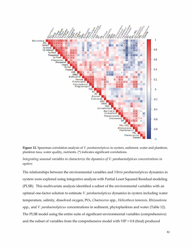
82

Figure 12. Spearman correlation analysis of V. parahaemolyticus in oysters, sediment, water and plankton,

plankton taxa, water quality, nutrients. (*) indicates significant correlations.

Integrating seasonal variables to characterize the dynamics of V. parahaemolyticus concentrations in

oysters

The relationships between the environmental variables and Vibrio parahaemolyticus dynamics in

oysters were explored using integrative analysis with Partial Least Squared Residual modeling

(PLSR). This multivariate analysis identified a subset of the environmental variables with an

optimal one-factor solution to estimate V. parahaemolyticus dynamics in oysters including water

temperature, salinity, dissolved oxygen, PO4, Chaetoceros spp., Helicotheca tamensis, Rhizosolenia

spp., and V. parahaemolyticus concentrations in sediment, phytoplankton and water (Table 12).

The PLSR model using the entire suite of significant environmental variables (comprehensive)

and the subset of variables from the comprehensive model with VIP > 0.8 (final) produced

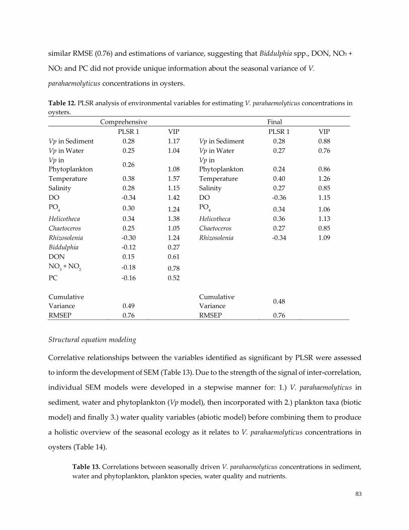
83

similar RMSE (0.76) and estimations of variance, suggesting that Biddulphia spp., DON, NO3 +

NO2 and PC did not provide unique information about the seasonal variance of V.

parahaemolyticus concentrations in oysters.

Table 12. PLSR analysis of environmental variables for estimating V. parahaemolyticus concentrations in

oysters.

Comprehensive Final

PLSR 1 VIP PLSR 1 VIP

Vp in Sediment 0.28 1.17 Vp in Sediment 0.28 0.88

Vp in Water 0.25 1.04 Vp in Water 0.27 0.76

Vp in

Phytoplankton 0.26

1.08

Vp in

Phytoplankton 0.24 0.86

Temperature 0.38 1.57 Temperature 0.40 1.26

Salinity 0.28 1.15 Salinity 0.27 0.85

DO -0.34 1.42 DO -0.36 1.15

PO4 0.30 1.24 PO

4 0.34 1.06

Helicotheca 0.34 1.38 Helicotheca 0.36 1.13

Chaetoceros 0.25 1.05 Chaetoceros 0.27 0.85

Rhizosolenia -0.30 1.24 Rhizosolenia -0.34 1.09

Biddulphia -0.12 0.27 DON 0.15 0.61

NO3 + NO

2 -0.18 0.78

PC -0.16 0.52 Cumulative

Variance 0.49

Cumulative

Variance 0.48

RMSEP 0.76 RMSEP 0.76

Structural equation modeling

Correlative relationships between the variables identified as significant by PLSR were assessed

to inform the development of SEM (Table 13). Due to the strength of the signal of inter-correlation,

individual SEM models were developed in a stepwise manner for: 1.) V. parahaemolyticus in

sediment, water and phytoplankton (Vp model), then incorporated with 2.) plankton taxa (biotic

model) and finally 3.) water quality variables (abiotic model) before combining them to produce

a holistic overview of the seasonal ecology as it relates to V. parahaemolyticus concentrations in

oysters (Table 14).

Table 13. Correlations between seasonally driven V. parahaemolyticus concentrations in sediment,

water and phytoplankton, plankton species, water quality and nutrients.

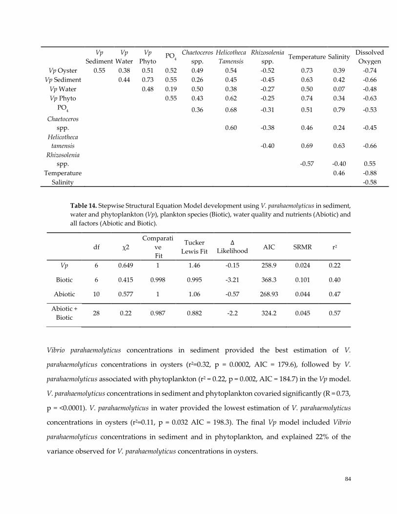
84

Vp

Sediment

Vp

Water

Vp

Phyto PO

4 Chaetoceros

spp.

Helicotheca

Tamensis

Rhizosolenia

spp. Temperature Salinity

Dissolved

Oxygen

Vp Oyster 0.55 0.38 0.51 0.52 0.49 0.54 -0.52 0.73 0.39 -0.74

Vp Sediment 0.44 0.73 0.55 0.26 0.45 -0.45 0.63 0.42 -0.66

Vp Water 0.48 0.19 0.50 0.38 -0.27 0.50 0.07 -0.48

Vp Phyto 0.55 0.43 0.62 -0.25 0.74 0.34 -0.63

PO4

0.36 0.68 -0.31 0.51 0.79 -0.53

Chaetoceros

spp. 0.60 -0.38 0.46 0.24 -0.45

Helicotheca

tamensis -0.40 0.69 0.63 -0.66

Rhizosolenia

spp. -0.57 -0.40 0.55

Temperature 0.46 -0.88

Salinity -0.58

Table 14. Stepwise Structural Equation Model development using V. parahaemolyticus in sediment,

water and phytoplankton (Vp), plankton species (Biotic), water quality and nutrients (Abiotic) and

all factors (Abiotic and Biotic).

df χ2

Comparati

ve

Fit

Tucker

Lewis Fit

∆ Likelihood

AIC SRMR r2

Vp 6 0.649 1 1.46 -0.15 258.9 0.024 0.22

Biotic 6 0.415 0.998 0.995 -3.21 368.3 0.101 0.40

Abiotic 10 0.577 1 1.06 -0.57 268.93 0.044 0.47

Abiotic +

Biotic 28 0.22 0.987 0.882 -2.2 324.2 0.045 0.57

Vibrio parahaemolyticus concentrations in sediment provided the best estimation of V.

parahaemolyticus concentrations in oysters (r2=0.32, p = 0.0002, AIC = 179.6), followed by V.

parahaemolyticus associated with phytoplankton (r2 = 0.22, p = 0.002, AIC = 184.7) in the Vp model.

V. parahaemolyticus concentrations in sediment and phytoplankton covaried significantly (R = 0.73,

p = <0.0001). V. parahaemolyticus in water provided the lowest estimation of V. parahaemolyticus

concentrations in oysters (r2=0.11, p = 0.032 AIC = 198.3). The final Vp model included Vibrio

parahaemolyticus concentrations in sediment and in phytoplankton, and explained 22% of the

variance observed for V. parahaemolyticus concentrations in oysters.

85

The biotic model, that incorporated plankton taxa with the Vp model, identified that Helicotheca

tamensis significantly covaried with Vibrio parahaemolyticus concentrations in oysters and

phytoplankton whereas Rhizosolenia spp. significantly covaried with V. parahaemolyticus

concentrations in oysters and sediment. Chaetoceros spp. did not significantly covary with V.

parahaemolyticus concentrations in oysters, sediment or phytoplankton and was not included in

the final biotic model. The addition of the plankton taxa to the Vp model improved the estimation

of V. parahaemolyticus concentrations in oysters from 22% to 40%. In the development of the abiotic

model, water temperature alone estimated 43.6% of the variance in V. parahaemolyticus

concentration in oysters. It was determined that water temperature was also correlated with the

variance in DO, salinity and PO4. An interaction between salinity and PO4 was accounted for in

the final abiotic and abiotic + biotic SEM.

The biotic and abiotic model combined produced a holistic SEM that accounted for the complex

combinations of abiotic and biotic variables that relate to the dynamics Vibrio parahaemolyticus

dynamics in oysters. Together, 57% of the variance observed in oysters was best fit by a

combination of V. parahaemolyticus concentration in sediment and phytoplankton, Helicotheca

tamensis and Rhizosolenia spp. concentrations, water temperature, PO4 and salinity (χ2 = 0.22, r2 =

0.55). V. parahaemolyticus concentration in water, Chaetoceros spp. and DO did not contribute to

the SEM model to explain V. parahaemolyticus dynamics in oysters and were not included in the

final model. Overall, water temperature had the strongest correlation to V. parahaemolyticus

concentrations in oysters (Figure 13). Water temperature was also significantly correlated with

the other variables in the abiotic and biotic models, though the strength of this correlation varied.

The variance of V. parahaemolyticus concentrations in sediment and phytoplankton were both

strongly correlated with V. parahaemolyticus concentration variation in oysters, though sediment

was stronger overall. Helicotheca tamensis and Rhizosolenia spp. improved model fit significantly

by fitting additional variance of V. parahaemolyticus concentrations. PO4 provided a stronger fit to

the model than salinity, however salinity was retained in the final SEM because of its contribution

to the variance of PO4. Substantial inter-correlation was also observed between plankton taxa,

water quality variables and V. parahaemolyticus in sediment and oysters.

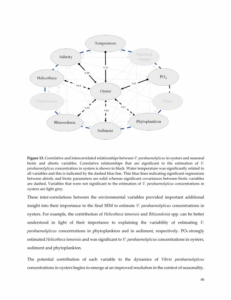
86

Figure 13. Correlative and intercorrelated relationships between V. parahaemolyticus in oysters and seasonal

biotic and abiotic variables. Correlative relationships that are significant to the estimation of V.

parahaemolyticus concentration in oysters is shown in black. Water temperature was significantly related to

all variables and this is indicated by the dashed blue line. Thin blue lines indicating significant regressions

between abiotic and biotic parameters are solid whereas significant covariances between biotic variables

are dashed. Variables that were not significant to the estimation of V. parahaemolyticus concentrations in

oysters are light grey.

These inter-correlations between the environmental variables provided important additional

insight into their importance to the final SEM to estimate V. parahaemolyticus concentrations in

oysters. For example, the contribution of Helicotheca tamensis and Rhizosolenia spp. can be better

understood in light of their importance to explaining the variability of estimating V.

parahaemolyticus concentrations in phytoplankton and in sediment, respectively. PO4 strongly

estimated Helicotheca tamensis and was significant to V. parahaemolyticus concentrations in oysters,

sediment and phytoplankton.

The potential contribution of each variable to the dynamics of Vibrio parahaemolyticus

concentrations in oysters begins to emerge at an improved resolution in the context of seasonality.

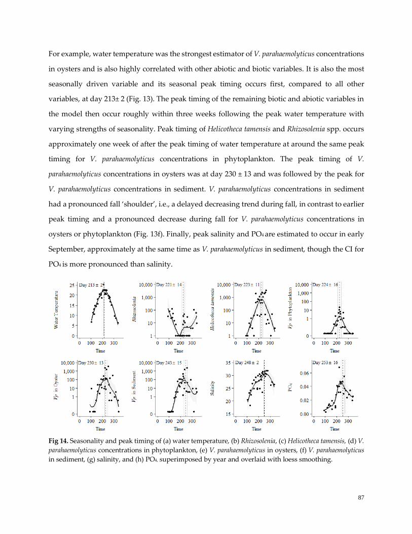
87

For example, water temperature was the strongest estimator of V. parahaemolyticus concentrations

in oysters and is also highly correlated with other abiotic and biotic variables. It is also the most

seasonally driven variable and its seasonal peak timing occurs first, compared to all other

variables, at day 213± 2 (Fig. 13). The peak timing of the remaining biotic and abiotic variables in

the model then occur roughly within three weeks following the peak water temperature with

varying strengths of seasonality. Peak timing of Helicotheca tamensis and Rhizosolenia spp. occurs

approximately one week of after the peak timing of water temperature at around the same peak

timing for V. parahaemolyticus concentrations in phytoplankton. The peak timing of V.

parahaemolyticus concentrations in oysters was at day 230 ± 13 and was followed by the peak for

V. parahaemolyticus concentrations in sediment. V. parahaemolyticus concentrations in sediment

had a pronounced fall ‘shoulder’, i.e., a delayed decreasing trend during fall, in contrast to earlier

peak timing and a pronounced decrease during fall for V. parahaemolyticus concentrations in

oysters or phytoplankton (Fig. 13f). Finally, peak salinity and PO4 are estimated to occur in early

September, approximately at the same time as V. parahaemolyticus in sediment, though the CI for

PO4 is more pronounced than salinity.

Fig 14. Seasonality and peak timing of (a) water temperature, (b) Rhizosolenia, (c) Helicotheca tamensis, (d) V.

parahaemolyticus concentrations in phytoplankton, (e) V. parahaemolyticus in oysters, (f) V. parahaemolyticus

in sediment, (g) salinity, and (h) PO4, superimposed by year and overlaid with loess smoothing.

88

Together, the correlations, inter-correlations and patterns of seasonality in the environmental

variables considered provide important insight into the seasonal microbial ecology of the GBE

and illustrates how the combined influence of each variable in light of seasonal timing and

correlative strength may contribute to the overall seasonality of Vibrio parahaemolyticus

concentration in oysters.

DISCUSSION

The emergence and establishment of Vibrio parahaemolyticus as a causative agent of shellfish-borne

illnesses in the Northeast United States has stimulated keen interest in understanding the coastal

ecosystem conditions that may influence this human health risk in this region. As V.

parahaemolyticus disease dynamics are changing worldwide, plankton dynamics, including the

distribution of plankton taxa and the frequency and intensity of harmful algal blooms, are also

changing concurrent with climate related changes in the marine environment (Cavicchioli et al.,

2019; Townhill et al., 2018; Baker-Austin et al., 2017; Grimes et al., 2014; Vezzulli et al., 2013).

Recent work based on a more limited set of environmental variables determined that V.

parahaemolyticus dynamics in the GBE are strongly influenced by seasonality and that patterns of

this seasonality are changing over time as V. parahaemolyticus concentrations are increasingly

elevated throughout the summer and are remaining high later into fall months (Hartwick et al.,

2019). Using an expanded suite of water quality and biological factors, we determined that V.

parahaemolyticus concentrations in sediment and phytoplankton, Helicotheca tamensis, Rhizosolenia

spp., water temperature, salinity and PO4 in the GBE are also seasonally driven in the GBE and

applied integrative multivariate analysis to illustrate how their seasonal dynamics may

ultimately contribute to the accumulation V. parahaemolyticus concentration in oysters. This

improved resolution of the environmental variables that associate with V. parahaemolyticus in the

GBE provides a basis to identify the environmental variables that contribute to the seasonality of

V. parahaemolyticus concentrations and to potentially better characterize the conditions that may

contribute to associate with human health risks in this region.

In the Northeast US, Vibrio parahaemolyticus concentrations and water temperature are highly

seasonal and V. parahaemolyticus dynamics most strongly correlate with water temperature as

89

reported for other temperate regions (Oberbeckman et al., 2011; Deter et al., 2010). In other regions

where V. parahaemolyticus dynamics are also seasonal yet driven by other environmental

conditions such as monsoons season, the relationship between temperature and V.

parahaemolyticus is not significant (Deepanjali et al., 2005). In New Hampshire, seasonality may

be one probable explanation for why regression modeling favors water temperature as the most

significant model parameter, among others (dissolved oxygen, pH, salinity and nutrients

including: NO3 + NO2, TDN and PO4) in the GBE, for estimating V. parahaemolyticus concentrations

in univariate regression. A complex combination of biological and physical environmental

variables certainly drives V. parahaemolyticus population dynamics, however, many of these

environmental variables are, in turn, driven mainly by seasonal temperature and therefore do not

contribute unique variance to a statistical model for describing seasonal ecology.

In this study, water temperature estimated 43.6% of the observed variability in V. parahaemolyticus

concentrations in oysters, and both the association with water temperature and the differing

patterns of seasonality varied between V. parahaemolyticus concentrations in oysters, sediment,

water, phyto and zooplankton. The influence of covarying environmental variables in statistical

models is likely one of many reasons why a complex array of environment variables has been

observed in studies around the world to correlate with Vibrio parahaemolyticus dynamics, though

other factors certainly relate to this, including differences between study design and analytic

methods. Differences in V. parahaemolyticus dynamics between matrices have been frequently

observed and some studies have applied models comprised of different environmental variables

to estimate V. parahaemolyticus in varying matrices (Nilsson et al., 2019, Deter et al., 2010). In the

GBE, the initial detection of V. parahaemolyticus in oysters and sediment began early in the year

and lasted through late fall though the peak timing of V. parahaemolyticus concentration dynamics

differed between matrices in terms of onset of detection and peak timing. The relationships

between matrices varied in significance, suggesting that some were more useful for explaining V.

parahaemolyticus concentrations in oysters.

There were similarities in the dynamics of Vibrio parahaemolyticus between matrices. For example,

V. parahaemolyticus concentrations in oysters were most strongly associated with V.

90

parahaemolyticus concentrations in sediment although there was also strong inter-correlation

between V. parahaemolyticus concentrations in sediment and phytoplankton. Though the

importance of the host shellfish to V. parahaemolyticus persistence is not clear (Lovell et al., 2017;

DePaola et al. 1990, 2003; Zimmerman et al. 2007), the accumulation of V. parahaemolyticus via

filter feeding of suspended sediments and plankton species has been frequently suggested (e.g.,

Froelich et al. 2013, Kaneko and Colwell et al., 1973, 1975). To account for these differences, we

applied seasonality analysis and peak timing to assess each variable for their contribution to the

overall seasonal ecology of V. parahaemolyticus in oysters in the GBE. For example, although V.

parahaemolyticus concentrations in sediment have the strongest correlative relationship to V.

parahaemolyticus concentrations in oysters, given the dynamics of sediment, diatoms on sediments

and in the water column, and the peak timing of V. parahaemolyticus in phytoplankton,

phytoplankton are also probably an important influence, perhaps in different ways or at different

times, on the seasonal pattern of V. parahaemolyticus in oysters. To further this point, V.

parahaemolyticus concentration in oysters peak within a week of V. parahaemolyticus concentrations

in phytoplankton whereas the pattern of seasonal emergence and gradually decreasing

concentrations in the fall is more similar between V. parahaemolyticus in sediment and oysters.

The variable temporal dynamics observed in Vibrio parahaemolyticus concentrations were similar

to the temporal dynamics of the GBE plankton community, where the patterns of community

assemblage tracked closely with water temperature, though the overall plankton abundance did

not. This was due in large part to individual taxa such as Skeletonema spp. that were present in

high numbers in early spring, or Fragilariopsis spp. and Navicula spp. that were present year-

round. Though Skeletonema spp. have also been reported as the major component of other

temperate water systems, it is also observed globally in marine systems (Canesi and Rynearson,

2016). Likewise, Fragilariopsis spp. has been reported in many locations around the world, though

it is generally associated with cold-water regions (Mock et al., 2017).

Helicotheca tamensis was significantly positively associated with V. parahaemolyticus dynamics in

oysters in the GBE. In the GBE it was often seen in single cell or short, straight square chains,

though it has been reported to form extended, twisted chains as well (Hernández-Becerril et al.,

91

2013). The ecology of H. tamensis is not well characterized, however it has been detected in a wide

range of environments including: the Bay of Fundy, the Baltic Sea, the Gulf of Mexico and the

Port of Recife in Brazil (Santiago et al., 2010, Halifors et al., 2004, Martin et al., 2001). In the Port

of Recife, which is classified as a eutrophic estuary, H. tamensis can dominate the plankton

community in summer months. The GBE is not considered a eutrophic estuary but H. tamensis

abundance can exceed >75% of the plankton community in late August and September, however

never at the densities seen elsewhere. Gilbert et al., (2012) and Furhman et al., (2008) suggests

that plankton community assemblage can be been attributed to a combination of factors, strongly

driven by water temperature, but modulated by individual temporal niches related to water

quality, nutrients or meteorological conditions that enable complex community dynamics in

temperate regions, similar to what is found for V. parahaemolyticus in our and other studies. The

co-occurring summer dynamics of H. tamensis and V. parahaemolyticus in oysters may indicate that

they share similar niche or physiological preferences, though these would require a more in-

depth study to fully characterize. Alternatively, H. tamensis abundance in the GBE could serve as

an easily measurable indicator of V. parahaemolyticus abundance in oysters in later summer and

early fall. It is also important to note that previous studies of the plankton taxa present in the GBE

do not mention H. tamensis (Jones, 2000; NAI, 1985). This could mean that H. tamensis is a recent

addition to the GBE plankton community and that the microbial community is being reshaped

via introduced species or changing ecological conditions.

Very little recent data on plankton communities and their dynamics in the GBE were available

prior to this study, so this study also provides an important update for this area. The plankton

community in the GBE appears to be diatom-dominated, as previously reported (Jones, 2000;

NAI, 1985). Though plankton species were detected in the water column from April through

December, on average the abundance was 6,700 cells/L and this varied strongly by time of the

year. Elevated concentrations from 10,000 to 35,000 cells/L were only seen in seven samples,

which were also those dominated by Cheatocerus spp. (n=5), Navicula spp. (n=1) or Skeletonema

spp. (n=1). Similarly, the concentration of chlorophyll-a was also generally low, with an average

of 6.3±4.5 µg/L. Together these findings suggest that the GBE has potentially limited water

column primary productivity and lack of relationships between Vibrio parahaemolyticus in oysters

92

with total abundance or the most abundant plankton taxa suggests that the use of plankton taxa

that do relate to V. parahaemolyticus dynamics would be better monitoring tools than chlorophyll-

a.

Chlorophyll-a is a widely used monitoring variable related to primary productivity in coastal

waters and, along with individual phytoplankton taxa, is a potentially useful tool for

characterizing risks associated with Vibrio parahaemolyticus in shellfish. There was also no

correlation found between chlorophyll-a and V. parahaemolyticus dynamics in the GBE. The

absence of a correlative relationship between chlorophyll-a and either V. parahaemolyticus

concentrations or phytoplankton dynamics found in this study has been reported elsewhere

(Takemura et al., 2014), suggesting again that phytoplankton taxa may be better monitoring

targets for tracking V. parahaemolyticus dynamics. Rhenstam-Holm et al. (2010) also observed a

negative relationship between Skeletonema spp. and Chaetoceros spp. blooms and V.

parahaemolyticus concentrations in their 2010 study, though Gilbert et al. (2012) identified an

incidental co-occurring bloom of V. parahaemolyticus and Chaetoceros spp. during their study

suggesting a positive bacterio-plankton interaction. There is work that has shown that V.

parahaemolyticus can also support a free-living lifestyle in the water column by subsisting off

nutrient-rich floccula or polysaccharide exudate (Takemura et al., 2014; Gilbert et al., 2010;

Venkataswaran, 1990) that may provide insight into why V. parahaemolyticus dynamics are not

related to chlorophyll-a or observed plankton blooms in the GBE. Given the relative low plankton

abundance observed in this study, it is important to consider that alternate factors might be more

strongly related to V. parahaemolyticus dynamics in the GBE, despite the reported importance of

phytoplankton blooms or chlorophyll-a reported elsewhere. In addition, the lack of a correlative

relationship between chlorophyll-a and overall plankton abundance or individual plankton taxa

identified in this study suggests alternate variables to chlorophyll-a should be considered to

monitor plankton dynamics in the GBE, at least at the size fraction of >53µm.

Nutrients are often monitored in coastal waters for many reasons and are potentially influential

variables that relate to both Vibrio parahaemolyticus and plankton dynamics (Paranjpye et al., 2015).

The contribution of nutrients to plankton and V. parahaemolyticus dynamics was also considered

93

as nutrient availability is likely one of the most important limiting factors of V. parahaemolyticus

dynamics in light of the metabolic demands based on its rapid growth rate (Espejo et al., 2017,

Turner et al., 2016, Johnson et al., 2013). The majority of nutrient variables were not seasonal or

significantly correlated to V. parahaemolyticus in oysters, sediment, plankton, and water or to

individual plankton taxa. The exception to this was NO3 + NO2 and PO4, both of which were

highly seasonal and strongly correlated with V. parahaemolyticus overall, and PO4 was determined

to be one of the most important variables to estimate V. parahaemolyticus in oysters in multivariate

analysis. An earlier study of V. parahaemolyticus concentrations in GBE water also reported PO4 as

a significant variable, in addition to water temperature, total and organic suspended solids (Jones

and Summer-Brason, 1998). Though the majority of nutrients were not significant to plankton or

V. parahaemolyticus dynamics in this study, previous studies (Blackwell and Oliver, 2008,

Oberbeckman et al., 2011) have reported positive correlations between Vibrio spp. and nutrients

such as TDN. It should be considered that the dynamics between nutrients, plankton and V.

parahaemolyticus are complex, and a lack of significance here could relate to some dimension of

these dynamics that was not accounted for in this study like the timing of nutrient loading events

and both plankton blooms and their decline (Trombetta et al., 2019; Cloern, 1996). For example,

low nutrient conditions may reflect the onset of declines in plankton blooms that can then cause

release of nutrients and polysaccharides from decaying plankton cells (Mühlenbruch et al., 2018).

A lack of significance between nutrient and V. parahaemolyticus concentrations could also reflect

the rapid turnover in nutrients during warm summer conditions and because their influence on

V. parahaemolyticus concentrations is an indirect interaction that does not consider the more direct

effect of nutrients on the plankton community (Gude, 1985). Future work with more frequent

sampling could provide an improved resolution of the contribution of nutrients to the microbial

community dynamics in the GBE.

Peak timing was used to assess the environmental variables in this study to determine how they

may individually contribute to the development of ideal conditions for Vibrio parahaemolyticus.

We determined that significant predictive variables peak both in advance and following the peak

timing of V. parahaemolyticus in oysters at day 230 (± 13). The photoperiod variable peaks first, on

the longest day of the year (day 170). This is followed by the peak timing of water temperature

94

(213 ± 2), then summer indicator phytoplankton Rhizosolenia spp. and Helicotheca tamensis, and V.

parahaemolyticus in phytoplankton, all potentially contributing to a hysteresis or loading of the

system that sets up optimal conditions for V. parahaemolyticus in oysters. Interestingly, especially

in relationship to filter feeding dynamics, the concentration of V. parahaemolyticus in the water

was poorly correlated with V. parahaemolyticus in oysters and sediment. It’s worth noting

however, that Chaetoceros spp. was the strongest estimator of V. parahaemolyticus in water. So,

although Chaetoceros spp. were the most abundant plankton taxa in the GBE in this study, they

did not strongly correlate with V. parahaemolyticus in oysters, suggesting Chaetoceros spp. may

have some undefined relation to overall V. parahaemolyticus dynamics in the full suite of

ecosystem matrices that exist in the study area. Finally, V. parahaemolyticus in sediment peak

timing occurs on day 243 ± 15 followed by salinity and PO4 and though the peak timing of V.

parahaemolyticus in oysters occurs ~2 weeks prior, elevated concentrations are still observed

during this time, suggesting that V. parahaemolyticus associated with sediments may be a key late

summer driver of the dynamics of oyster V. parahaemolyticus concentrations.

Previous modeling efforts in the GBE determined that the characteristics of seasonality combined

with water temperature, pH, salinity and photoperiod improved the estimation of Vibrio

parahaemolyticus incidence and concentration predictions in the GBE (Hartwick et al., 2019;

Urquhart et al., 2016). The relationship with photoperiod and community dynamics in

phytoplankton and V. parahaemolyticus was also observed by Gilbert et al. (2012) and Nilsson et

al. (2019) in other coastal areas. Moreover, the importance of lags upwards of a month to

effectively estimate V. parahaemolyticus concentrations was recently shown by Davis et al., (2019).

Data in this study were collected either monthly or biweekly, whereas V. parahaemolyticus can

replicate every eight minutes under ideal conditions. Traditional methods for lag analysis and

cross correlation could provide an improved resolution of these lagged effects on V.

parahaemolyticus with more frequent sampling and fine-scale temporal resolution. However, in

this study, the application of harmonic regression and peak timing demonstrates how biological

complexities and limitations of sampling frequency can be accounted for and provide an in-depth

characterization of the ecological dynamics of plankton and V. parahaemolyticus in a highly

seasonal estuary.

95

CONCLUSIONS

The seasonality of an extended suite of water quality, meteorological conditions and

biological community variables was assessed to characterize the interactions of plankton and

Vibrio parahaemolyticus dynamics oysters in the GBE. The overall dynamics of V. parahaemolyticus

were highly seasonal and patterns of peak timing and the onset of detection varied considerably,

suggesting complex ecological linkages between co-occurring plankton, water quality and V.

parahaemolyticus dynamics. The relationships observed between plankton community abundance,

blooms and V. parahaemolyticus concentrations in phyto- and zooplankton suggests that indicators

such as chlorophyll-a and plankton blooms may not be informative leading indicators of V.

parahaemolyticus dynamics in oysters in the GBE. However, the shared seasonality of water

temperature, salinity, PO4, Helicotheca tamensis, and V. parahaemolyticus in sediment and

phytoplankton provides a first step towards a more in-depth description of the biotic and abiotic

ecology of V. parahaemolyticus. Though a complex combination of environmental variables

certainly drives V. parahaemolyticus dynamics, including location specific ecology and potentially

population specific genetics/genomics (Froelich and Noble, 2016; Shapiro and Polz, 2014), this

work provides a first step towards the characterization of how plankton and other environmental

variables contribute to the overarching seasonality and are drivers that may be contributing to

the changing dynamics of V. parahaemolyticus in oysters in the Northeast US. The overall analytical

approach is a useful and potentially transferable framework for similar studies in other temperate

coastal areas.

Supplementary Materials: Figure 1: Seasonal Environmental variables and peak timing. Figure 2:

Environmental variables with limited seasonal periodicity. Table S1: Environmental Variables with

minimal seasonality based on photoperiod and harmonic regression modeling.

Author Contributions: Conceptualization, MAH, AB, ENN and SHJ.; methodology, MAH, NL, AB and

SHJ.; software, MAH, AB.; validation, CAW, VSC, ENN and SHJ.; formal analysis, MAH; resources, CAW,

VSC, SHJ.; data curation, MAH and AB.; writing—original MAH, AB; writing—review and editing, CAW,

VSC, ENN and SHJ.; visualization, MAH and AB.; supervision, SJH.; funding acquisition, CAW, VSC, SHJ.

Funding: The authors gratefully acknowledge partial funding support from the National Science

Foundation EPSCoR IIA-1330641, USDA National Institute of Food and Agriculture Hatch NH00574,

NH00609 (accession 233555), and NH00625 (accession 1004199), and the National Oceanic and Atmospheric

Administration College Sea Grant program and New Hampshire Sea Grant program grants R/CE-137,

R/SSS-2, R/HCE- 3

96

Acknowledgments: The authors would like to thank Jennifer Mahoney, Meg Striplin, Brian Schuster,

Crystal Ellis, Jong Yu, Eliot Jones, Michael Taylor, Ashley Marcinkiewicz, Feng Xu, Tom Gregory, Chris

Peters, Jackie Lemaire, Sarah Richards, Emily Schulz, and Elizabeth Deyett for their help with sampling,

sample processing, detection analysis, and database management. Also, Alexandra Kulinkina and Tania

M. Alarcon Falconi for support with implementing harmonic regression analysis and peak timing

calculations in the R environment.

Conflicts of Interest: The authors declare no conflict of interest. The funders had no role in the design of

the study; in the collection, analyses, or interpretation of data; in the writing of the manuscript, or in the

decision to publish the results.

97

References

Hartwick, M. A., Urquhart, E. A., Whistler, C. A., Cooper, V. S., Naumova, E. N., & Jones, S. H. (2019).

Forecasting Seasonal Vibrio parahaemolyticus Concentrations in New England Shellfish.

International journal of environmental research and public health, 16(22), 4341.

Lovell, C. R. Ecological fitness and virulence features of Vibrio parahaemolyticus in estuarine

environments. Applied microbiology and biotechnology 2017, 101(5), 1781-1794.

Urquhart, E. A.; Jones, S. H.; Jong, W. Y.; Schuster, B. M.; Marcinkiewicz, A. L.; Whistler, C. A.; Cooper,

V. S. Environmental conditions associated with elevated Vibrio parahaemolyticus concentrations in

Great Bay Estuary, New Hampshire. PloS one 2016, 11(5), e0155018.

Turner, J. W.; Malayil, L.; Guadagnoli, D.; Cole, D.; Lipp, E. K. Detection of Vibrio parahaemolyticus,

Vibrio vulnificus and Vibrio cholerae with respect to seasonal fluctuations in temperature and

plankton abundance. Environmental microbiology 2014, 16(4), 1019-1028.

Martinez-Urtaza, J.; Blanco-Abad, V.; Rodriguez-Castro, A.; Ansede-Bermejo, J.; Miranda, A.;

Rodriguez-Alvarez, M. X.; Ecological determinants of the occurrence and dynamics of Vibrio

parahaemolyticus in offshore areas. The ISME Journal 2012, 6(5), 994–1006.

Vezzulli, L.; Pezzati, E.; Moreno, M.; Fabiano, M.; Pane, L.; Pruzzo, C.; VibrioSea Consortium. Benthic

ecology of Vibrio spp. and pathogenic Vibrio species in a coastal Mediterranean environment (La

Spezia Gulf, Italy). Microbial ecology 2009, 58(4), 808-818.

Jones, S.; Summer-Brason, B. Incidence and detection of pathogenic Vibrio spp. in a northern New

England estuary, USA. Journal of Shellfish Research 1998, 17, 1665–1669.

DePaola, A.; Hopkins, L.H.; Peeler, J.T.; Wentz, B.; McPhearson, R.M. Incidence of Vibrio parahaemolyticus

in US coastal waters and oysters. Appl. Environ. Microbiol. 1990, 1;56(8), 2299-302.

Kaneko, T., & Colwell, R. R. Ecology of Vibrio parahaemolyticus in Chesapeake Bay. Journal of

Bacteriology 1973, 113(1), 24-32

Erken M, Lutz C, McDougald D. 2015. Interactions of Vibrio spp. with zooplankton. microbiolspec 3(3):

doi:10.1128/microbiolspec.VE-0003-2014

Vezzulli, L., Colwell, R. R., & Pruzzo, C. Ocean warming and spread of pathogenic Vibrios in the aquatic

environment. Microbial ecology 2013, 65(4), 817-825.

Hughes, S. N., Greig, D. J., Miller, W. A., Byrne, B. A., Gulland, F. M., & Harvey, J. T. (2013). Dynamics

of Vibrio with virulence genes detected in Pacific harbor seals (Phoca vitulina richardii) off

California: implications for marine mammal health. Microbial ecology, 65(4), 982-994.

Martinez-Urtaza, J.; Lozano-Leon, A.; Varela-Pet, J.; Trinanes, J.; Pazos, Y.; Garcia-Martin, O.

Environmental determinants of the occurrence and distribution of Vibrio parahaemolyticus in the

rias of Galicia, Spain. Appl. Environ. Microbiol. 2008, 74(1), 265-274.

Alipour, M., Issazadeh, K., & Soleimani, J. (2014). Isolation and identification of Vibrio parahaemolyticus

from seawater and sediment samples in the southern coast of the Caspian Sea. Comparative

clinical pathology, 23(1), 129-133.


environmental persistence and clinical nature of the human pathogen Vibrio vulnificus. Appl.


Froelich, B., Ayrapetyan, M., & Oliver, J. D. (2013). Integration of Vibrio vulnificus into marine

aggregates and its subsequent uptake by Crassostrea virginica oysters. Appl. Environ. Microbiol.,

79(5), 1454-1458.

Parveen, S.; Hettiarachchi, K.A.; Bowers, J.C.; Jones, J.L.; Tamplin, M.L.; McKay, R.; Beatty, W.;

Brohawn, K.; DaSilva, L.V.; DePaola, A. Seasonal distribution of total and pathogenic Vibrio

parahaemolyticus in Chesapeake Bay oysters and waters. International journal of food

microbiology 2008, 128(2), 354-361.

98

DePaola, A.; Nordstrom, J.L.; Bowers, J.C.; Wells, J.G.; Cook, D.W. Seasonal abundance of total and

pathogenic Vibrio parahaemolyticus in Alabama oysters. Appl. Environ. Microbiol. 2003, 69:1521–

1526.

Johnson, C. N. (2013). Fitness factors in vibrios: a mini-review. Microbial ecology, 65(4), 826-851.

Zimmerman, A. M.; DePaola, A.; Bowers, J. C.; Krantz, J. A.; Nordstrom, J. L.; Johnson, C. N.; Grimes,

D. J. Variability of total and pathogenic Vibrio parahaemolyticus densities in northern Gulf of Mexico

water and oysters. Appl. Environ. Microbiol 2007, 73(23), 7589-7596.

Kaneko, T., & Colwell, R. R. (1977). The annual cycle of Vibrio parahaemolyticus in Chesapeake Bay.

Microbial ecology, 4(2), 135-155.

Caburlotto, G.; Haley, B. J.; Lleò, M. M.; Huq, A.; Colwell, R. R. Serodiversity and ecological distribution

of Vibrio parahaemolyticus in the Venetian Lagoon, Northeast Italy. Environmental microbiology

reports 2010, 2(1), 151-157.

Takemura, A.; Chien, D.; Polz, M. Associations and dynamics of Vibrionaceae in the environment, from

the genus to the population level. Frontiers in Microbiology 2014, 5(38).

Turner, J. W.; Good, B.; Cole, D.; Lipp, E. K. Plankton composition and environmental factors contribute

to Vibrio seasonality. The ISME journal 2009, 3(9), 1082.

Paranjpye, R. N.; Nilsson, W. B.; Liermann, M.; Hilborn, E.D.; George, B.J.; Li, Q.; Bill, B.D.; Trainer,

V.L.; Strom, M.S.; Sandifer, P.A. Environmental influences on the seasonal distribution of Vibrio

parahaemolyticus in the Pacific Northwest of the USA. FEMS microbiology ecology 2015, 91(12),

121.

Gilbert, J.A.; Steele, J.A.; Caporaso, J.G.; Steinbrück, L.; Reeder, J.; Temperton, B.; Huse, S.; McHardy,

A.C.; Knight, R.; Joint, I.; Somerfield, P. Defining seasonal marine microbial community dynamics.

The ISME journal 2012, 6(2), p.298.

Grimes, D. J.; Ford, T. E.; Colwell, R. R.; Baker-Austin, C.; Martinez-Urtaza, J.; Subramaniam, A.;

Capone, D. G. Viewing marine bacteria, their activity and response to environmental drivers from

orbit: satellite remote sensing of bacteria. Microbial Ecology 2014, 67(3), 489–500.

Asplund, Maria E., Ann‐Sofi Rehnstam‐Holm, Vijay Atnur, Pendru Raghunath, Vasudevan Saravanan,

Karolina Härnström, Betty Collin, Indrani Karunasagar, and Anna Godhe. "Water column

dynamics of Vibrio in relation to phytoplankton community composition and environmental

conditions in a tropical coastal area." Environmental microbiology 13, no. 10 (2011): 2738-2751.

Beveridge, O. S., Petchey, O. L., & Humphries, S. (2010). Direct and indirect effects of temperature on

the population dynamics and ecosystem functioning of aquatic microbial ecosystems. Journal of

Animal Ecology, 79(6), 1324-1331.

Kaneko, T., & Colwell, R. R. (1975). Incidence of Vibrio parahaemolyticus in Chesapeake Bay. Appl.


Cavicchioli, R., Ripple, W.J., Timmis, K.N., Azam, F., Bakken, L.R., Baylis, M., Behrenfeld, M.J.,

Boetius, A., Boyd, P.W., Classen, A.T., Crowther, T.W., Danovaro, R., Foreman, C.M., Huisman,

J., Hutchins, D.A., Jansson, J.K., Karl, D.M., Koskella, B., Welch, M.D.B., Martiny, J.B.H., Moran,

M.A., Orphan, V.J., Reay, D.S., Remais, J.V., Rich, V.I., Singh, B.K., Stein, L.Y., Stewart, F.J.,

Sullivan, M.B., van Oppen, M.J.H., Weaver, S.C., Webb, E.A. Webster, N.S. Scientists’ warning to

humanity: microorganisms and climate change, Nature Reviews Microbiology, (2019) 569,586,17;

9. https://doi.org/10.1038/s41579-019-0222-5

Townhill, B.L., Tinker, J., Jones, M., Pitois, S., Creach, V., Simpson, S.D., Dye, S., Bear, E., Pinnegar, J.K.,

Harmful algal blooms and climate change: exploring future distribution changes, ICES Journal of

Marine Science, Volume 75, Issue 6, November-December 2018, Pages 1882–1893,

https://doi.org/10.1093/icesjms/fsy113

https://doi.org/10.1093/icesjms/fsy113

99

Baker-Austin, C., Trinanes, J., Gonzalez-Escalona,. N & Martinez-Urtaza, J. Non-Cholera Vibrios: The

Microbial Barometer of Climate Change. Trends Microbiol. (2017) Jan;25(1):76-84. doi:

10.1016/j.tim.2016.09.008.

Vezzulli, L., Colwell, R.R. & Pruzzo, C. Microb Ecol (2013) 65: 817. https://doi.org/10.1007/s00248-012-

0163-2

Kaysner, C.; DePaola, A. (2004) Chapter 9: Vibrio. In:BAM Council (eds) Bacteriological analytical

manual online. US Food and Drug Administration. Available at

https://www.fda.gov/food/laboratory-methods-food/bam-vibrio (accessed June 17, 2019).

Leland, N.J. , J.F. Haney and W. Young, Into the light: A method and device for plankton separation

(manuscript in preparation).

USEPA. 2003. Sampling and Analytical Procedures for GLNPO’s Open Lake Water Quality Survey of

the Great Lakes. U.S. Environmental Protection Agency, Great Lakes National Program Office,

Chicago, IL.

Leland, N.J. and Haney, J.F. (2018) Alternative Methods for Analysis of Cyanobacterial Populations in

Drinking Water Supplies: Fluorometric and Toxicological Applications Using Phycocyanin.

Journal of Water Resource and Protection, 10, 740-761. https://doi.org/10.4236/jwarp.2018.108042

Baker, A.L. et al. 2012. Phycokey -- an image based key to Algae (PS Protista), Cyanobacteria, and other

aquatic objects. University of New Hampshire Center for Freshwater Biology.

http://cfb.unh.edu/phycokey/phycokey.htm 3 Oct 2019.

Cooper, S. & Dolan, C. A Guide to Common Gulf of Maine, Great Bay Coast Watch National Sea Grant

College Program of the U.S. Department of Commerce’s National Oceanic and Atmospheric

Administration (NOAA) grant #NA060AR4170109 to the NH Sea Grant College Program. NH Sea

Grant publication UNHMP-M-SG-06-35 Summer 2006 Additional copies are available from: NH

Sea Grant Communications Kingman Farm/University of New Hampshire Durham, NH

R Core Team (2019). R: A language and environment for statistical computing. R Foundation for

Statistical Computing, Vienna, Austria. URL https://www.R-project.org/.

Oksanen, F. J., Blanchet, G., Friendly, M., Kindt, R., Legendre, P., McGlinn, D., Minchin, P.R., O'Hara,

B., Simpson, G.L., Solymos, P., Stevens, M.H., Szoecs, E., & Wagner, E. (2019). vegan: Community

Ecology Package. R package version 2.5-6. https://CRAN.R-project.org/package=vegan

Naumova, E.N.; MacNeill, I.B. Seasonality Assessment for Biosurveillance. In: Advances in Statistical

Methods for the Health Sciences. Auget JL, Balakrishnan N, Mesbah M, Molenberghs G, eds..

Birkhauser. 2007. pp437–450.

Alarcon Falconi, T.M.; Cruz, M.; Naumova, E.N. The shift in seasonality of legionellosis in the U.S.

Epidemiol Infect. 2018, 146, 1824-1833.

Jones, S. H. (2000). A technical characterization of estuarine and coastal New Hampshire. PREP Reports

and Publications

Piscataqua Region Estuaries Partnership, "State of Our Estuaries Report 2018" (2017). PREP Reports &

Publications. 391. https://scholars.unh.edu/prep/391Normandeau Associates, Inc. Piscataqua

River Ecological Studies, 1979 Monitoring Studies, Report No. 10 for Public Service Company of

New Hampshire..,Bedford, N.H. 502pp

Hartwick, M., and Jones, S. H. Vibrio parahaemolyticus Population Dynamics Within an Estuarine

Microbial Community. 2016. Poster presentation. International Symposium on Microbial Ecology,

Montreal, Canada.

Oberbeckmann, S.; Wichels, A.; Wiltshire, K. H.; Gerdts, G. Occurrence of Vibrio parahaemolyticus and

Vibrio alginolyticus in the German Bight over a seasonal cycle. Antonie Van Leeuwenhoek 2011,

100(2), 291-307.

http://cfb.unh.edu/phycokey/phycokey.htm 3%20Oct%202019

https://www.r-project.org/

https://cran.r-project.org/package=vegan

100

Deter, J., Solen, L., Antoine, V., Jaufrey, J., Annick, D., Dominique, H.H. (2010). Ecology of pathogenic

and non‐pathogenic Vibrio parahaemolyticus on the French Atlantic coast. Effects of temperature,

salinity, turbidity and chlorophyll a. Environmental microbiology, 12(4), 929-937.

Deepanjali, A., Kumar, H., Karunasagar, I., Karunasagar, I. Seasonal Variation in Abundance of Total

and Pathogenic Vibrio parahaemolyticus in Oysters along the Southwest Coast of India. Applied and

Environmental Microbiology. (2005) 71, 7. http://aem.asm.org/content/71/7/3575.abstract

Canesi, K. L., & Rynearson, T. A. (2016). Temporal variation of Skeletonema community composition

from a long-term time series in Narragansett Bay identified using high-throughput DNA

sequencing. Marine Ecology Progress Series, 556, 1-16.

Mock, T., Otillar, R.P., Strauss, J., McMullan, M., Paajanen, P., Schmutz, J., Salamov, A., Sanges, R.,

Toseland, A., Ward, B.J. and Allen, A.E., 2017. Evolutionary genomics of the cold-adapted diatom

Fragilariopsis cylindrus. Nature, 541(7638), p.536.

Hernández-Becerril, D. U., Nelson, N. R., Barón-Campis, S. A., & Moreno-Gufiérrez, S. P. (2013).

Morphological study of two closely related marine planktonic diatoms: Bellerochea malleus and

Helicotheca tamesis. Cryptogamie, Algologie, 34(3), 245-255.

Santiago, Marilene Felipe, Maria da Glória Gonçalves Silva-Cunha, Sigrid Neumann-Leitão, Kátia

Muniz Pereira da Costa, Gislayne Cristina Borges Palmeira, Porto Neto, Fernando de Figueiredo,

and Fabiana Santana Nunes. "Phytoplankton dynamics in a highly eutrophic estuary in tropical

Brazil." Brazilian Journal of Oceanography 58, no. 3 (2010): 189-205.

Martin, J. L.; LeGresley, M. M. ; Strain, P. M. (2001). Phytoplankton monitoring in the Western Isles

region of the Bay of Fundy during 1997-98. Canadian Technical Report of Fisheries and Aquatic

Sciences 2349. 4: 1-85. [details]

Hällfors, G. (2004). Checklist of Baltic Sea Phytoplankton Species (including some heterotrophic

protistan groups). Baltic Sea Environment Proceedings. No. 95: 210 pp., available online at

http://helcom.fi/Lists/Publications/BSEP95.pdf

Fuhrman, J. A., Steele, J. A., Hewson, I., Schwalbach, M. S., Brown, M. V., Green, J. L., & Brown, J. H.

(2008). A latitudinal diversity gradient in planktonic marine bacteria. Proceedings of the National

Academy of Sciences, 105(22), 7774-7778.


cohesive units. Trends in microbiology, 22(5), 235-247.

Nilsson, W. B., Paranjpye, R. N., Hamel, O. S., Hard, C., & Strom, M. S. (2019). Vibrio parahaemolyticus

risk assessment in the Pacific Northwest: it's not what's in the water. FEMS microbiology ecology,

95(4), fiz027.

Rehnstam-Holm, A. S., Godhe, A., Härnström, K., Raghunath, P., Saravanan, V., Collin, B., ... &

Karunasagar, I. (2010). Association between phytoplankton and Vibrio spp. along the southwest

coast of India: a mesocosm experiment. Aquatic Microbial Ecology, 58(2), 127-139

Venkateswaran, K., Kiiyukia, C., Nakanishi, K., Nakano, H., Matsuda, O., & Hashimoto, H. (1990). The

role of sinking particles in the overwintering process of Vibrio parahaemolyticus in a marine

environment. FEMS Microbiology Ecology, 6(2), 159-166.

Espejo, R. T., García, K., & Plaza, N. (2017). Insight into the origin and evolution of the Vibrio

parahaemolyticus pandemic strain. Frontiers in microbiology, 8, 1397.

Turner, J. W., Berthiaume, C. T., Morales, R., Armbrust, E. V., & Strom, M. S. (2016). Genomic evidence

of adaptive evolution in emergent Vibrio parahaemolyticus ecotypes. Elem Sci Anth, 4.

Blackwell, K. D.; Oliver, J. D. The ecology of Vibrio vulnificus, Vibrio cholerae, and Vibrio parahaemolyticus

in North Carolina estuaries. The Journal of Microbiology 2008, 46(2), 146-153.

Cloern, J. E. (1996). Phytoplankton bloom dynamics in coastal ecosystems: a review with some general

lessons from sustained investigation of San Francisco Bay, California. Reviews of Geophysics,

34(2), 127-168.

101

Trombetta, T., Vidussi, F., Mas, S., Parin, D., Simier, M., & Mostajir, B. (2019). Water temperature drives

phytoplankton blooms in coastal waters. PloS one, 14(4), e0214933.

Mühlenbruch, M., Grossart, H. P., Eigemann, F., & Voss, M. (2018). Mini‐review: Phytoplankton‐

derived polysaccharides in the marine environment and their interactions with heterotrophic

bacteria. Environmental microbiology, 20(8), 2671-2685.

Güde, H. (1985). Influence of phagotrophic processes on the regeneration of nutrients in two-stage

continuous culture systems. Microbial ecology, 11(3), 193-204.

Froelich, B. A.; Noble, R. T. Vibrio bacteria in raw oysters: managing risks to human health.

Philosophical Transactions of the Royal Society B: Biological Sciences 2016, 371(1689), 20150209.

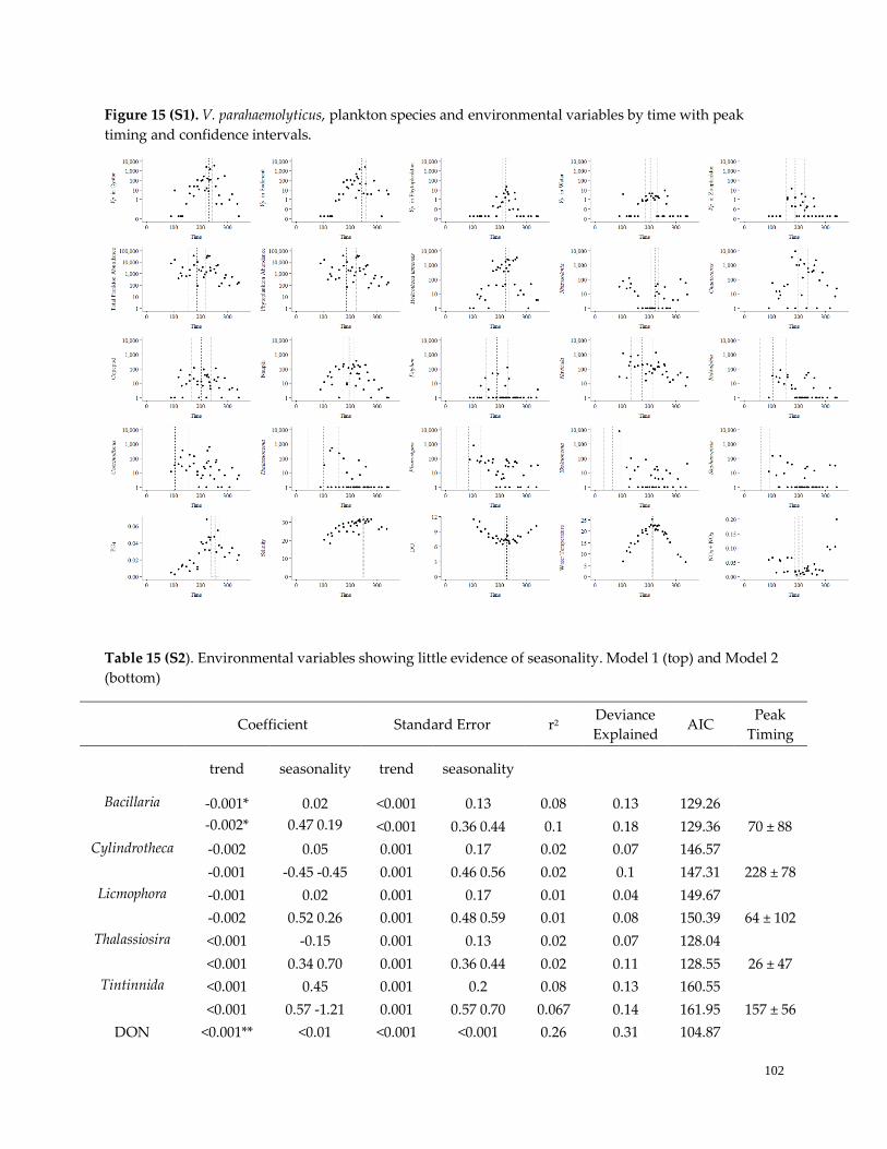
102

Figure 15 (S1). V. parahaemolyticus, plankton species and environmental variables by time with peak

timing and confidence intervals.

Table 15 (S2). Environmental variables showing little evidence of seasonality. Model 1 (top) and Model 2

(bottom)

Coefficient Standard Error r2

Deviance

Explained AIC

Peak

Timing

trend seasonality trend seasonality

Bacillaria -0.001* 0.02 <0.001 0.13 0.08 0.13 129.26

-0.002* 0.47 0.19 <0.001 0.36 0.44 0.1 0.18 129.36 70 ± 88

Cylindrotheca -0.002 0.05 0.001 0.17 0.02 0.07 146.57

-0.001 -0.45 -0.45 0.001 0.46 0.56 0.02 0.1 147.31 228 ± 78

Licmophora -0.001 0.02 0.001 0.17 0.01 0.04 149.67

-0.002 0.52 0.26 0.001 0.48 0.59 0.01 0.08 150.39 64 ± 102

Thalassiosira <0.001 -0.15 0.001 0.13 0.02 0.07 128.04

<0.001 0.34 0.70 0.001 0.36 0.44 0.02 0.11 128.55 26 ± 47

Tintinnida <0.001 0.45 0.001 0.2 0.08 0.13 160.55

<0.001 0.57 -1.21 0.001 0.57 0.70 0.067 0.14 161.95 157 ± 56

DON <0.001** <0.01 <0.001 <0.001 0.26 0.31 104.87

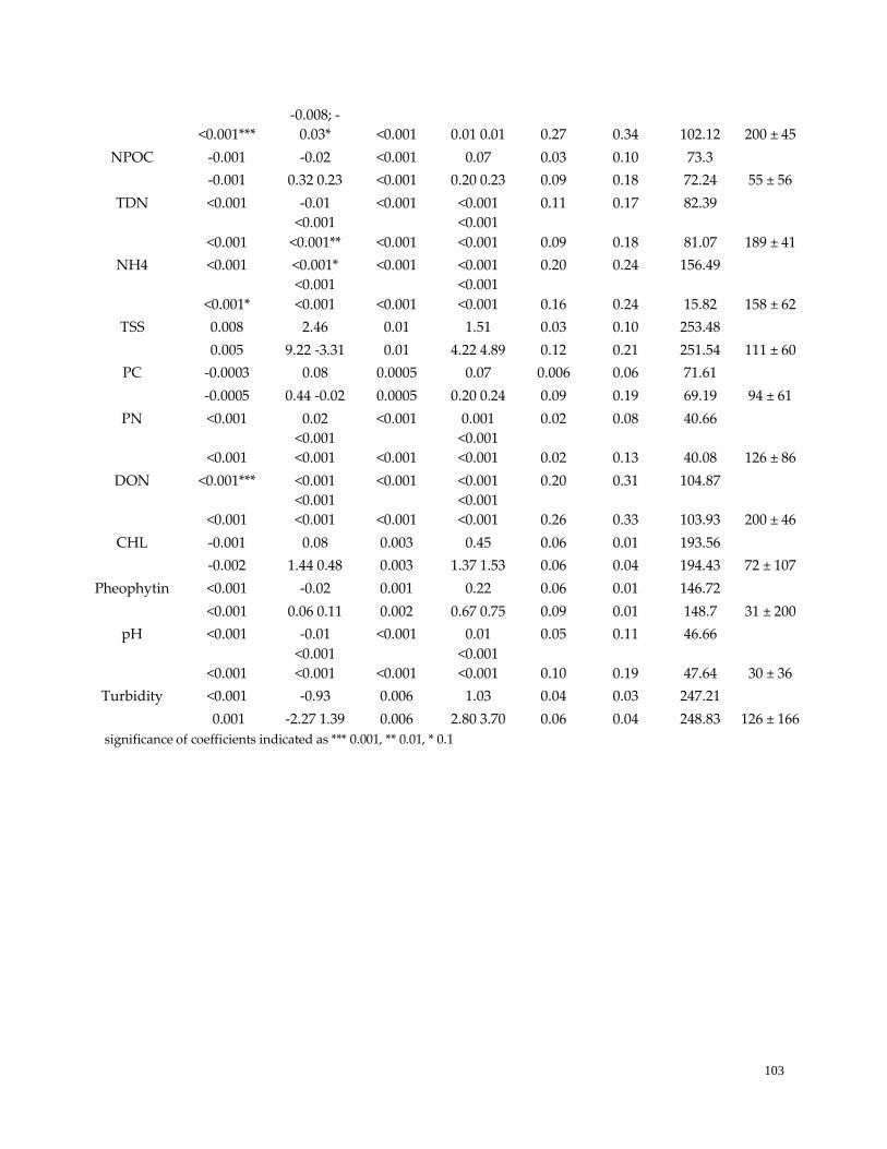
103

significance of coefficients indicated as *** 0.001, ** 0.01, * 0.1

<0.001***

-0.008; -

0.03* <0.001 0.01 0.01 0.27 0.34 102.12 200 ± 45

NPOC -0.001 -0.02 <0.001 0.07 0.03 0.10 73.3

-0.001 0.32 0.23 <0.001 0.20 0.23 0.09 0.18 72.24 55 ± 56

TDN <0.001 -0.01 <0.001 <0.001 0.11 0.17 82.39

<0.001

<0.001

<0.001** <0.001

<0.001

<0.001 0.09 0.18 81.07 189 ± 41

NH4 <0.001 <0.001* <0.001 <0.001 0.20 0.24 156.49

<0.001*

<0.001

<0.001 <0.001

<0.001

<0.001 0.16 0.24 15.82 158 ± 62

TSS 0.008 2.46 0.01 1.51 0.03 0.10 253.48

0.005 9.22 -3.31 0.01 4.22 4.89 0.12 0.21 251.54 111 ± 60

PC -0.0003 0.08 0.0005 0.07 0.006 0.06 71.61

-0.0005 0.44 -0.02 0.0005 0.20 0.24 0.09 0.19 69.19 94 ± 61

PN <0.001 0.02 <0.001 0.001 0.02 0.08 40.66

<0.001

<0.001

<0.001 <0.001

<0.001

<0.001 0.02 0.13 40.08 126 ± 86

DON <0.001*** <0.001 <0.001 <0.001 0.20 0.31 104.87

<0.001

<0.001

<0.001 <0.001

<0.001

<0.001 0.26 0.33 103.93 200 ± 46

CHL -0.001 0.08 0.003 0.45 0.06 0.01 193.56

-0.002 1.44 0.48 0.003 1.37 1.53 0.06 0.04 194.43 72 ± 107

Pheophytin <0.001 -0.02 0.001 0.22 0.06 0.01 146.72

<0.001 0.06 0.11 0.002 0.67 0.75 0.09 0.01 148.7 31 ± 200

pH <0.001 -0.01 <0.001 0.01 0.05 0.11 46.66

<0.001

<0.001

<0.001 <0.001

<0.001

<0.001 0.10 0.19 47.64 30 ± 36

Turbidity <0.001 -0.93 0.006 1.03 0.04 0.03 247.21

0.001 -2.27 1.39 0.006 2.80 3.70 0.06 0.04 248.83 126 ± 166

104

Chapter 3

Adaptations of an Environmental Population of Vibrio parahaemolyticus in the Great Bay Estuary

Meghan Hartwicka,b , Cheryl Whistler a,b, Vaughn Cooper a,d, Stephen Jones a,c aNortheast Center for Vibrio Disease and Ecology, University of New Hampshire, Durham, NH;

[email protected] bDepartment of Molecular, Cellular, and Biomedical Sciences, University of New Hampshire,

Durham, NH; [email protected] cDepartment of Natural Resources and the Environment, University of New Hampshire, Durham,

NH; [email protected] dDepartment of Microbiology and Molecular Genetics, University of Pittsburgh School of

Medicine, Pittsburgh, PA; [email protected]

ABSTRACT

Vibrio parahaemolyticus is a leading cause of foodborne illness, and the intrinsic link it has with the

environment it inhabits has been well studied and characterized. A wide range of environmental

conditions and ecological interactions has been reported to influence, or at least correlate with V.

parahaemolyticus concentrations. The complexity of this ecology coupled with the notable

differences observed in drivers of V. parahaemolyticus dynamics has led to the observation that a

combination of environmental factors including fine-scale differentiation of the V.

parahaemolyticus population into genetically distinct sub populations may contribute conditions

that differentially promote human health risk. V. parahaemolyticus isolates collected over the

course of one year from oysters, phytoplankton and zooplankton at two sites in the Great Bay

estuary (GBE) were sequenced with Illumina Hi-Seq and Oxford Nanopore Technology to assess

V. parahaemolyticus for evidence of local adaptation or ecotype differentiation between isolates by

site, matrix and season. Forty-one unique sequence types (ST) were identified in the population

and sixteen of these were previously reported on the pubMLST V. parahaemolyticus ST database.

Though lineage most strongly predicted genetic diversity between isolates in the GBE, evidence

of horizontal exchange of plasmids and niche specific-genetic content was observed, and this

combination of genetic content through lineage and lifestyle masked potential ecotype

differentiation. The recently proposed V. parahaemolyticus cgMLST and isolates in ST 12, 49, 57

and 114 collected from locations outside the GBE were also compared to determine if an

ecological signal could be identified in evolutionary patterns.




105

1. INTRODUCTION

Vibrio parahaemolyticus is a leading cause of foodborne illness and is naturally occurring in the

environment where it persists through nutrient cycling and contributes to the food web. Whereas

most strains are believed to be non-pathogenic, a subset of the species can cause gastroenteritis

and septicemia in humans (FDA, 2005). Strains that cause human disease are most often

contracted from the consumption of raw or undercooked shellfish and other seafood in warm

water regions and more recently in temperate regions (FDA, 2005; McLaughlin et al., 2005). The

emergence and establishment of V. parahaemolyticus as a causative agent of shellfish-borne

illnesses in the Northeast United States has stimulated keen interest in understanding the

environmental conditions that may influence human health risk in this region.

The ecology of Vibrio parahaemolyticus has been well studied and characterized (eg: Lovell, 2017;

Davis et al., 2017; Urquhart et al. 2016; Lopez-Hernandez et al., 2015; Turner et al., 2014;Martinez-

Urtaza et al. 2012; Oberbeckman et al., 2011; Vezulli et al., 2009; Baker-Austin et al. 2010,

Deepanjali et al., 2005, Jones and Summer-Brason 1998, DePaola et al., 1990, Colwell et al., 1973).

Whether shellfish are a preferred environment for V. parahaemolyticus remains unclear, however

because of their commercial importance, the shellfish-V. parahaemolyticus relationship is the most

frequently studied interaction (Lovell et al., 2017; DePaola et al. 1990, 2003; Zimmerman et al.

2007). Filter feeding of suspended material is the most likely route by which V. parahaemolyticus

becomes concentrated in shellfish (e.g., Froelich et al. 2013). Given this, V. parahaemolyticus

associated with copepods and chitinous phytoplankton are frequently studied as they may relate

to V. parahaemolyticus dynamics in shellfish (Caburlotto et al., 2010; Takemura et al., 2014, Turner,

2009 and 2014, Paranjpye et al., 2015, Gilbert et al., 2012, Grimes et al., 2014 Martinez-Urtaza et

al., 2012, Asplunde et al. 2011, Beveridge et al., 2010, Kaneko and Colwell, 1975).

Concentrations of Vibrio parahaemolyticus in the Great Bay estuary (GBE) from different

environmental matrices have distinctly different seasonal patterns and peak timing, especially

between V. parahaemolyticus in oysters, phyto and zooplankton (Hartwick et al., in prep)

suggesting that the dynamics of V. parahaemolyticus may vary by niche in the environment. These

differences in V. parahaemolyticus dynamics between matrices have been observed elsewhere in

106

both its variable detection rate as well as the environmental conditions that V. parahaemolyticus is

associated with (Takemura et al., 2014). This type of ecological differentiation has been studied

as it may relate to underlying genetic differences in V. parahaemolyticus. Johnson et al., (2012) and

Shapiro and Polz (2014) reported V. parahaemolyticus strains from similar environmental niches

were more similar in genetic content and allelic diversity than they were to strains that were

isolated from different environmental conditions. Genetically distinct sub-populations of V.

parahaemolyticus constrained by geographic barriers have also been observed (Yang et al., 2019;

Cui et al., 2015). Further, Keymer et al., (2007) and Hunt et al., (2008) identified potential

differentiation in other Vibrio spp. by allelic variation or variable genome content that was linked

to the distinct ecological-niche from which strains were isolated. These observations are part of

the basis for proposing that Vibrio parahaemolyticus populations may be structured into ecological

species, or ecotypes.

Ecotypes can be understood as sub-populations that interact with other strains within their niche

but have limited exposure to V. parahaemolyticus that do not interact within the same

microhabitats in the environment. Because of this genetic isolation and the niche-specific

conditions, strains that inhabit similar niches will have more similar allelic diversity and

accessary genomes (Freidman, Alm and Shapiro, 2012). V. parahaemolyticus is an ideal candidate

to investigate the potential of differentiation by micro-environment within a population. The

genome is generally composed of two circular chromosomes with ~5,000 genes (Makino et al.,

2003), approximately half of which are conserved, and the remaining genome can be highly

variable even between closely related strains (Gonzalez-Escalono et al., 2016). This variable

content can be acquired through multiple routes including horizontal gene transfer mediated by

conjugation between individuals, transduction via phage and chitin-induced competence (Le

Roux and Blokesch, 2018). Allelic diversity of the material already present in the genome can be

introduced via homologous recombination and mutation (Bobay and Ochman, 2017, Ceccarelli et

al., 2013; Johnson, 2013). These mechanisms contribute to the standing genetic diversity of

housekeeping genes, core genes and variable genome content and may result in the

differentiation of sub populations of V. parahaemolyticus into ecotypes if the rate of gene flow is

variable within environments compared to between environments (Shapiro and Polz, 2014,

107

Cordero and Polz, 2014, Hunt et al., 2008, Johnson et al., 2006; Cohan et al., 2001). This can in turn

provide information about the ecological drivers that are shaping the population based on

prevalence of that shared characteristic to contribute to persistence within the local population

(Metzger and Blokesch, 2014).

Given the high amount of genetic diversity of Vibrio parahaemolyticus within the GBE (Ellis et al.,

2012) and the variability of seasonal dynamics of V. parahaemolyticus (Hartwick et al., 2019; in

prep.), isolates from oysters, phyto and zooplankton collected throughout 2014 were assembled

using a combination of Illumina and Oxford Nanopore Technology (ONT) for whole genome

analysis to determine how the observed environmental variability could be better understood in

light of patterns of underlying genetic population diversity. In addition to their potential

contribution to the accumulation of V. parahaemolyticus in oysters, V. parahaemolyticus isolates

from phyto and zooplankton were of interest to determine if differences in diversity could be

detected from isolates directly cultured from chitin-rich niches based on the potential of chitin-

induced competence to facilitate horizontal gene transfer.

An important yet under studied challenge for developing broadly useful methods for monitoring

and forecasting V. parahaemolyticus risk is the influence of unique sets of environmental variables

on the location and population specific genetic and genomic adaptations that lead to V.

parahaemolyticus population variations at regional and even the harvest area scales (Noble and

Froelich, 2016). Therefore, providing context to the relationship between genetic diversity and the

environment is an important direction to better understand how the environment shapes V.

parahaemolyticus dynamics in order to identify the conditions that are associated with human-

health risk. The potential for location-specific adaptations of V. parahaemolyticus to the ecology of

the GBE observed in this study is an important step to connect environmental conditions to

population dynamics and provides new targets for identifying the environmental variables that

influence V. parahaemolyticus concentrations in oysters.

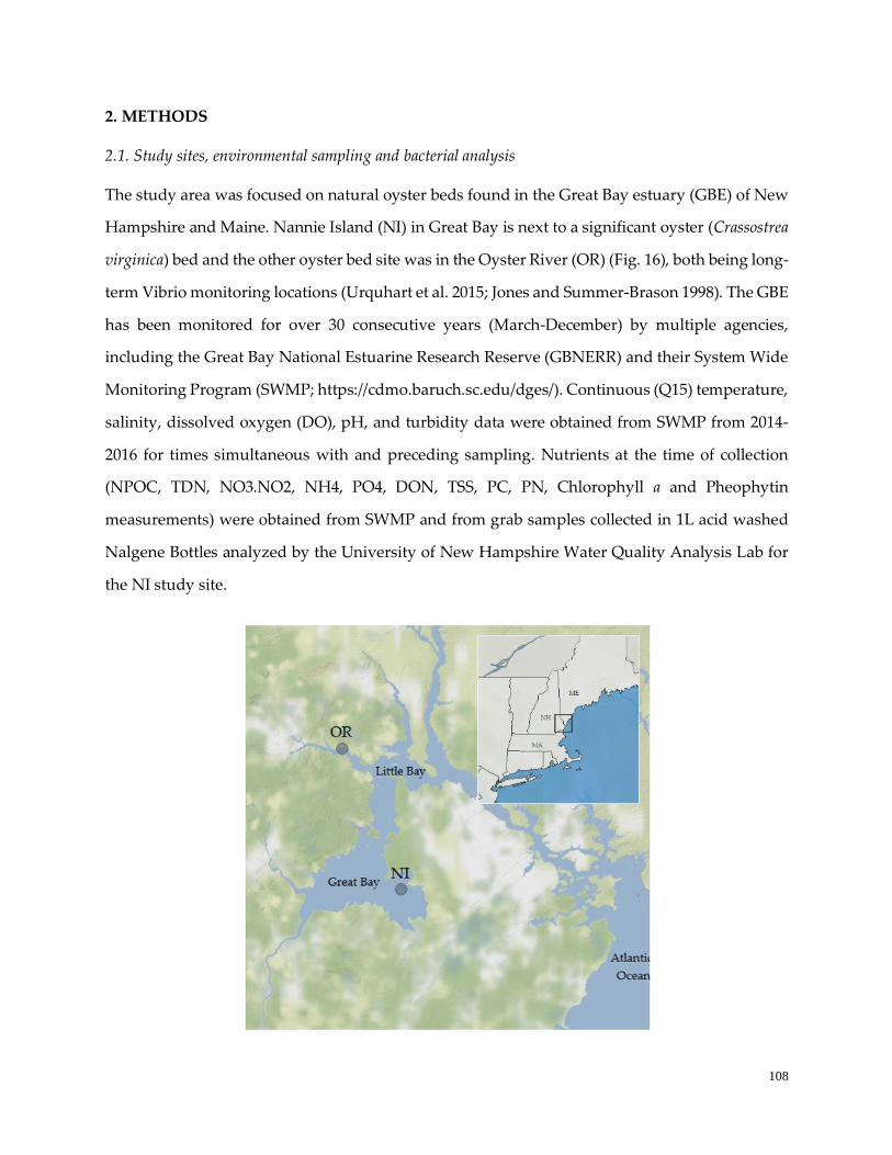
108

2. METHODS

2.1. Study sites, environmental sampling and bacterial analysis

The study area was focused on natural oyster beds found in the Great Bay estuary (GBE) of New

Hampshire and Maine. Nannie Island (NI) in Great Bay is next to a significant oyster (Crassostrea

virginica) bed and the other oyster bed site was in the Oyster River (OR) (Fig. 16), both being long-

term Vibrio monitoring locations (Urquhart et al. 2015; Jones and Summer-Brason 1998). The GBE

has been monitored for over 30 consecutive years (March-December) by multiple agencies,

including the Great Bay National Estuarine Research Reserve (GBNERR) and their System Wide

Monitoring Program (SWMP; https://cdmo.baruch.sc.edu/dges/). Continuous (Q15) temperature,

salinity, dissolved oxygen (DO), pH, and turbidity data were obtained from SWMP from 2014-

2016 for times simultaneous with and preceding sampling. Nutrients at the time of collection

(NPOC, TDN, NO3.NO2, NH4, PO4, DON, TSS, PC, PN, Chlorophyll a and Pheophytin

measurements) were obtained from SWMP and from grab samples collected in 1L acid washed

Nalgene Bottles analyzed by the University of New Hampshire Water Quality Analysis Lab for

the NI study site.

109

Fig. 16. The GBE Study area on the border of Maine and New Hampshire. OR = Oyster River; NI = Nannie

Island

Oyster and plankton samples were collected concurrently with water temperature, salinity, pH

and DO using YSI 6600 and EXO multiprobe sondes (Yellow Springs Instruments, Yellow

Springs, Ohio), during low tide from the NI and OR study sites. Plankton samples were collected

using a 53 µm mesh net (Aquatic Instruments). Oyster, phyto- and zooplankton samples were

processed and analyzed for V. parahaemolyticus detection according to previously published

methods (Hartwick et al., 2019) with alkaline peptone water enrichment, Vibrio CHROMAgar

and the FDA established PCR and MPN calculations at UNH Jackson Estuarine Lab (JEL).

Probable Vibrio isolates were confirmed as V. parahaemolyticus by PCR detection of the tlh gene

(Urquhart et al., 2016, Hartwick et al., 2019, Kaysner and DePaola, 2004).

2.2 Illumina sequencing

2.2.1 Isolate selection and Ssquencing

All isolates from 2014 oyster, phytoplankton and zooplankton were considered for genomic

analysis. Isolates from were cultured overnight in HI broth and genomic DNA from each isolate

was isolated with the DNeasy Blood and Tissue Kit (QIAGEN, Valencia, CA). DNA quality and

concentrations were evaluated with NanoDrop 1000 (Thermo Scientific, Rockford, IL). The final

concentration of high-quality extractions was quantified using a Qubit double-stranded DNA HS

assay kit and a Qubit 2.0 fluorometer (Life Technologies, Grand Island, NY). Libraries for Illumina

sequencing were generated using the TruSeq Kit (Illumina). One hundred and five unique

isolates were submitted to the UNH Hubbard Genome Center for Illumina-Hi Seq 250bp paired-

end sequencing.

2.2.2 Assembly and annotation

Sequenced forward and reverse reads were quality checked with FASTQC (Page, 2010). Adapter

and low-quality reads were trimmed with Trimmomatic (Bolger et al., 2014) then assembled with

SPAdes (Nurk et al., 2013). Assembly quality was assessed with Quast (Gurevich et al., 2013). A

custom python script was used to remove contigs with <10x coverage. Twenty isolates were not

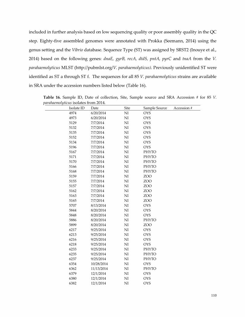
110

included in further analysis based on low sequencing quality or poor assembly quality in the QC

step. Eighty-five assembled genomes were annotated with Prokka (Seemann, 2014) using the

genus setting and the Vibrio database. Sequence Type (ST) was assigned by SRST2 (Inouye et al.,

2014) based on the following genes: dnaE, gyrB, recA, dtdS, pntA, pyrC and tnaA from the V.

parahaemolyticus MLST (http://pubmlst.org/V. parahaemolyticus). Previously unidentified ST were

identified as ST a through ST f. The sequences for all 85 V. parahaemolyticus strains are available

in SRA under the accession numbers listed below (Table 16).

Table 16. Sample ID, Date of collection, Site, Sample source and SRA Accession # for 85 V.

parahaemolyticus isolates from 2014.

Isolate ID Date Site Sample Source Accession #

4974 6/20/2014 NI OYS

4973 6/20/2014 NI OYS

5129 7/7/2014 NI OYS

5132 7/7/2014 NI OYS

5135 7/7/2014 NI OYS

5152 7/7/2014 NI OYS

5134 7/7/2014 NI OYS

5196 7/7/2014 NI OYS

5167 7/7/2014 NI PHYTO

5171 7/7/2014 NI PHYTO

5170 7/7/2014 NI PHYTO

5166 7/7/2014 NI PHYTO

5168 7/7/2014 NI PHYTO

5159 7/7/2014 NI ZOO

5155 7/7/2014 NI ZOO

5157 7/7/2014 NI ZOO

5162 7/7/2014 NI ZOO

5163 7/7/2014 NI ZOO

5165 7/7/2014 NI ZOO

5707 8/13/2014 NI OYS

5844 8/20/2014 NI OYS

5848 8/20/2014 NI OYS

5886 8/20/2014 NI PHYTO

5899 8/20/2014 NI ZOO

6217 9/25/2014 NI OYS

6213 9/25/2014 NI OYS

6216 9/25/2014 NI OYS

6218 9/25/2014 NI OYS

6233 9/25/2014 NI PHYTO

6235 9/25/2014 NI PHYTO

6237 9/25/2014 NI PHYTO

6354 10/28/2014 NI OYS

6362 11/13/2014 NI PHYTO

6379 12/1/2014 NI OYS

6380 12/1/2014 NI OYS

6382 12/1/2014 NI OYS

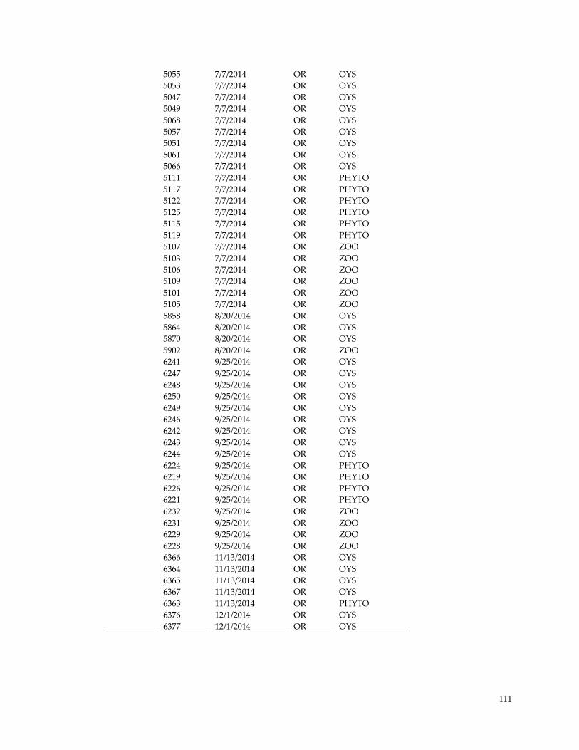
111

5055 7/7/2014 OR OYS

5053 7/7/2014 OR OYS

5047 7/7/2014 OR OYS

5049 7/7/2014 OR OYS

5068 7/7/2014 OR OYS

5057 7/7/2014 OR OYS

5051 7/7/2014 OR OYS

5061 7/7/2014 OR OYS

5066 7/7/2014 OR OYS

5111 7/7/2014 OR PHYTO

5117 7/7/2014 OR PHYTO

5122 7/7/2014 OR PHYTO

5125 7/7/2014 OR PHYTO

5115 7/7/2014 OR PHYTO

5119 7/7/2014 OR PHYTO

5107 7/7/2014 OR ZOO

5103 7/7/2014 OR ZOO

5106 7/7/2014 OR ZOO

5109 7/7/2014 OR ZOO

5101 7/7/2014 OR ZOO

5105 7/7/2014 OR ZOO

5858 8/20/2014 OR OYS

5864 8/20/2014 OR OYS

5870 8/20/2014 OR OYS

5902 8/20/2014 OR ZOO

6241 9/25/2014 OR OYS

6247 9/25/2014 OR OYS

6248 9/25/2014 OR OYS

6250 9/25/2014 OR OYS

6249 9/25/2014 OR OYS

6246 9/25/2014 OR OYS

6242 9/25/2014 OR OYS

6243 9/25/2014 OR OYS

6244 9/25/2014 OR OYS

6224 9/25/2014 OR PHYTO

6219 9/25/2014 OR PHYTO

6226 9/25/2014 OR PHYTO

6221 9/25/2014 OR PHYTO

6232 9/25/2014 OR ZOO

6231 9/25/2014 OR ZOO

6229 9/25/2014 OR ZOO

6228 9/25/2014 OR ZOO

6366 11/13/2014 OR OYS

6364 11/13/2014 OR OYS

6365 11/13/2014 OR OYS

6367 11/13/2014 OR OYS

6363 11/13/2014 OR PHYTO

6376 12/1/2014 OR OYS

6377 12/1/2014 OR OYS

112

2.3 Gene content and pangenome analysis

Pangenome analysis was conducted with Roary (Page et al., 2015), BLASTP identity was set to

90% and consideration of genes to be core (or variable) was based on the presence of the gene in

at least 98% percent of isolates (~83/85). Gene Ontology (GO) was assigned using Blast+ (Altschul

et al., 1990) and the Uniref90 and UniprotKB databases (The UniProt Consortium, 2019). The

highest identity match from BLASTX of was selected based on 100 results. Gene function was

assigned with GO.db (Carlson, 2019) and GO categories were assessed using the highest order

GO terms within the classification of biological processes, molecular function and cellular

process.

2.4 Nanopore sequencing

Previously extracted gDNA (section 2.2.1) from representative isolates of each clonal cluster were

re-sequenced using the Nanopore ligation sequencing kit 1D (R9 version) for MinION

sequencing. Unicycler (Wick et al., 2017) was used to produce Nanopore and Illumina hybrid

assemblies and annotated with Prokka (Seemann, 2014). Assembly quality were evaluated with

Quast (Gurevich et al., 2013) and visualized with Bandage (Wick et al., 2015). Ten isolates were

assembled to a minimum coverage of 30x and resolved to two chromosomes with hybrid ONT

and Illumina sequenced reads.

2.5 Allelic diversity

Hybrid Nanopore-Illumina sequenced and assembled isolates were aligned with Minimap (Li,

2018) and annotated variant call files (VCF) were constructed with SAMtools and BCFtools (Li et

al., 2009) or a custom bash pipeline of gene alignment files from Roary (Page et al., 2015) and

SNP-sites (Page et al., 2016). VCFtools (Danecek et al., 2011) was used to filter SNPS by quality >

60. Phylogenetics relationships between isolates in the study were assessed using MLST, core

genes and variable genes aligned in MAFFT (Katoh & Standley, 2013) and PRANK (Löytynoja,

A. 2014). Maximum likelihood trees were constructed in RAxML (Stamatakis, 2014).

Relationships were visualized using the ggtree package developed for R (Yu et al., 2017).

113

2.6 Local adaptation

2.6.1 Chromosomal distribution of core genome content

The core genome content identified by Roary (Page et al., 2015) analysis was compared to the V.

parahaemolyticus core genome (Gonzelez-Escalono et al., 2016). The FASTA and GBK files of V.

parahaemolyticus isolates resolved to 2 chromosomes and categorized as ‘complete’ from NCBI

(Coordinators, N.R., 2016) were accessed on 9/19/2019. Gene location of the core genes in the GBE

V. parahaemolyticus population was compared with chromosomal gene location from the

geographically distinct closed NCBI V. parahaemolyticus genomes.

2.6.2 Global ST and local adaptation

Custom scripts combining the SRA query tool (Leinonen et al., 2010) and SRST2 (Inouye

et al., 2014) were used to query to the Vibrio parahaemolyticus short-read archive for genomes with

ST identified in the eighty-five genomes included in this study. Seven isolates with matching ST

were identified, assembled and annotated using the pipeline specified in section 2.2.2. Gene

content and allelic diversity were analyzed as described in section 2.3 to look for evidence of

genetic change in lineages that were isolated within the GBE compared to matching ST from other

regions.

2.7 Genome wide association studies

Genome wide association studies (GWAS) between genomic content, function or allelic diversity

and ST, date, site and matrix was performed using a combination of Scoary (Brynildsrud et al.,

2016), TopGo (Rahnenfuhrer, 2019) and multivariate analysis with Multiple Permutation

Response Procedure (MRPP), Non Metric Ordination Analysis (NMDS) with vegan: Community

Ecology Package, 2.5-2 (Oksanen et al., 2018), and Indicator Species Analysis (ISA): indicspecies

(De Caceres and Legendre, 2009) in R version 3.5.3 (R Core Team, 2019).

3. Results

Eighty-five isolates from oysters, phyto and zooplankton were collected from June to

December in 2014 and sequenced with Illumina Hi-Seq to a minimum 10x coverage (Figure 17).

The average number of base pairs per genome was 5,080,909 ± 82,643 and these resolved to an

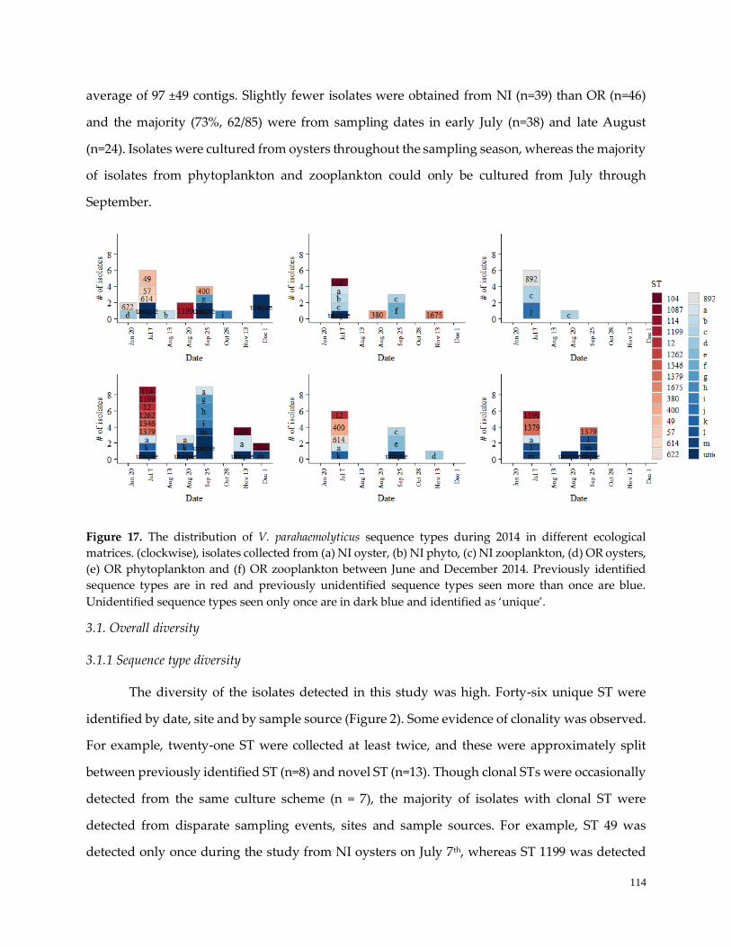
114

average of 97 ±49 contigs. Slightly fewer isolates were obtained from NI (n=39) than OR (n=46)

and the majority (73%, 62/85) were from sampling dates in early July (n=38) and late August

(n=24). Isolates were cultured from oysters throughout the sampling season, whereas the majority

of isolates from phytoplankton and zooplankton could only be cultured from July through

September.

Figure 17. The distribution of V. parahaemolyticus sequence types during 2014 in different ecological

matrices. (clockwise), isolates collected from (a) NI oyster, (b) NI phyto, (c) NI zooplankton, (d) OR oysters,

(e) OR phytoplankton and (f) OR zooplankton between June and December 2014. Previously identified

sequence types are in red and previously unidentified sequence types seen more than once are blue.

Unidentified sequence types seen only once are in dark blue and identified as ‘unique’.

3.1. Overall diversity

3.1.1 Sequence type diversity

The diversity of the isolates detected in this study was high. Forty-six unique ST were

identified by date, site and by sample source (Figure 2). Some evidence of clonality was observed.

For example, twenty-one ST were collected at least twice, and these were approximately split

between previously identified ST (n=8) and novel ST (n=13). Though clonal STs were occasionally

detected from the same culture scheme (n = 7), the majority of isolates with clonal ST were

detected from disparate sampling events, sites and sample sources. For example, ST 49 was

detected only once during the study from NI oysters on July 7th, whereas ST 1199 was detected

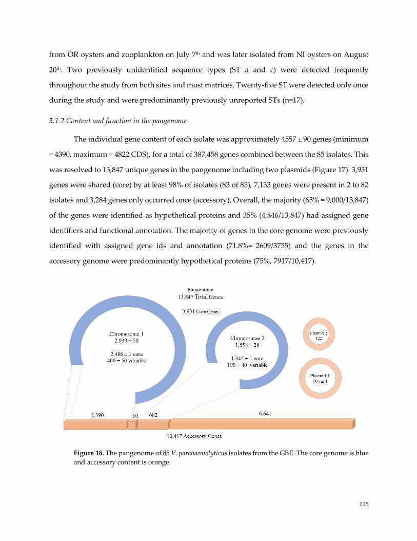
115

from OR oysters and zooplankton on July 7th and was later isolated from NI oysters on August

20th. Two previously unidentified sequence types (ST a and c) were detected frequently

throughout the study from both sites and most matrices. Twenty-five ST were detected only once

during the study and were predominantly previously unreported STs (n=17).

3.1.2 Content and function in the pangenome

The individual gene content of each isolate was approximately 4557 ± 90 genes (minimum

= 4390, maximum = 4822 CDS), for a total of 387,458 genes combined between the 85 isolates. This

was resolved to 13,847 unique genes in the pangenome including two plasmids (Figure 17). 3,931

genes were shared (core) by at least 98% of isolates (83 of 85), 7,133 genes were present in 2 to 82

isolates and 3,284 genes only occurred once (accessory). Overall, the majority (65% = 9,000/13,847)

of the genes were identified as hypothetical proteins and 35% (4,846/13,847) had assigned gene

identifiers and functional annotation. The majority of genes in the core genome were previously

identified with assigned gene ids and annotation (71.8%= 2609/3755) and the genes in the

accessory genome were predominantly hypothetical proteins (75%, 7917/10,417).

Figure 18. The pangenome of 85 V. parahaemolyticus isolates from the GBE. The core genome is blue

and accessory content is orange.

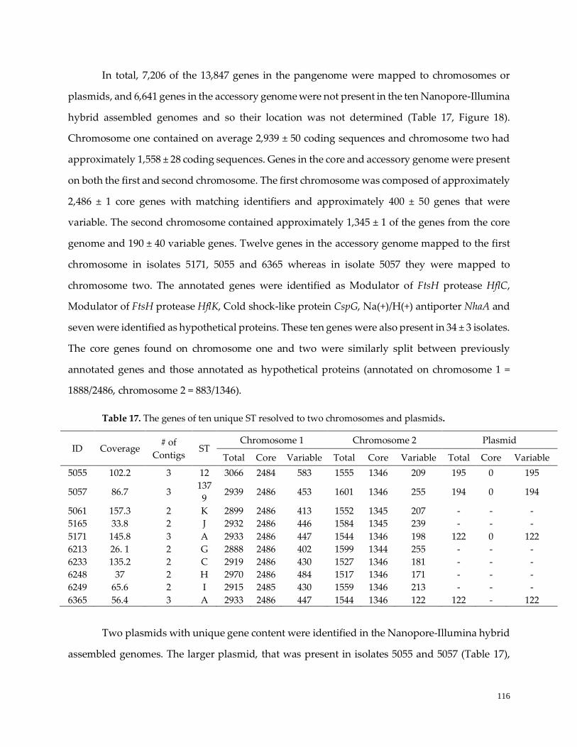
116

In total, 7,206 of the 13,847 genes in the pangenome were mapped to chromosomes or

plasmids, and 6,641 genes in the accessory genome were not present in the ten Nanopore-Illumina

hybrid assembled genomes and so their location was not determined (Table 17, Figure 18).

Chromosome one contained on average 2,939 ± 50 coding sequences and chromosome two had

approximately 1,558 ± 28 coding sequences. Genes in the core and accessory genome were present

on both the first and second chromosome. The first chromosome was composed of approximately

2,486 ± 1 core genes with matching identifiers and approximately 400 ± 50 genes that were

variable. The second chromosome contained approximately 1,345 ± 1 of the genes from the core

genome and 190 ± 40 variable genes. Twelve genes in the accessory genome mapped to the first

chromosome in isolates 5171, 5055 and 6365 whereas in isolate 5057 they were mapped to

chromosome two. The annotated genes were identified as Modulator of FtsH protease HflC,

Modulator of FtsH protease HflK, Cold shock-like protein CspG, Na(+)/H(+) antiporter NhaA and

seven were identified as hypothetical proteins. These ten genes were also present in 34 ± 3 isolates.

The core genes found on chromosome one and two were similarly split between previously

annotated genes and those annotated as hypothetical proteins (annotated on chromosome 1 =

1888/2486, chromosome 2 = 883/1346).

Table 17. The genes of ten unique ST resolved to two chromosomes and plasmids.

ID Coverage # of

Contigs ST

Chromosome 1 Chromosome 2 Plasmid

Total Core Variable Total Core Variable Total Core Variable

5055 102.2 3 12 3066 2484 583 1555 1346 209 195 0 195

5057 86.7 3 137

9 2939 2486 453 1601 1346 255 194 0 194

5061 157.3 2 K 2899 2486 413 1552 1345 207 - - -

5165 33.8 2 J 2932 2486 446 1584 1345 239 - - -

5171 145.8 3 A 2933 2486 447 1544 1346 198 122 0 122

6213 26. 1 2 G 2888 2486 402 1599 1344 255 - - -

6233 135.2 2 C 2919 2486 430 1527 1346 181 - - -

6248 37 2 H 2970 2486 484 1517 1346 171 - - -

6249 65.6 2 I 2915 2485 430 1559 1346 213 - - -

6365 56.4 3 A 2933 2486 447 1544 1346 122 122 - 122

Two plasmids with unique gene content were identified in the Nanopore-Illumina hybrid

assembled genomes. The larger plasmid, that was present in isolates 5055 and 5057 (Table 17),

117

was also part of the genome of isolates 5101, 5103 and 5155. The smaller plasmid, that was present

in 5171 and 6365, was also in the genomes of isolates 5051, 5109, 5115, 5858, 6241 and 6364. In the

larger plasmid, 21/194 genes had gene ids and functional annotation whereas the majority (89%,

173/194) of genes were annotated as hypothetical proteins. Similarly, there were 13/122 genes in

the smaller plasmid with gene ids and annotation, whereas the majority (89%, 109/122) of genes

were annotated as hypothetical proteins.

9,510 genes in the pangenome were annotated in the uniprotKB database and 5100 of these

also had functional gene ontology (GO) for either molecular (n= 3742), cellular (n= 2377) or

biological function (n=2050). Only 741 genes were annotated for all function GO groups. The

majority of genes annotated in the cellular component group were related to cellular structure

function and maintenance of cell membrane (GO:0016021, n=1288), cytosol (GO:0005737, n = 370)

and ATP-binding (GO:0043190, n = 36). Multiple genes were also related to bacterial flagellum

development (GO:0009288, n = 25), type II (GO:0015627, n = 3) and type III secretion systems

(GO:0030257, n = 3). Approximately one third (1279 genes) annotated with molecular function

GO were involved in binding (GO = GO:0005488). DNA binding (GO:0003677, n=549), ATP

binding (GO:0005524, n= 201) and RNA binding (GO:0003723, n = 47) represented the majority of

genes related to this function, but various metal ion binding functions were also present. The

other major group within molecular function involved genes related to catalytic activity. The

majority of genes in this group were involved with transferase activity (GO:0016740, n=281),

hydrolase activity (GO:0016787, n = 139), and sixteen genes were involved with recombinase

activity (GO:0000150).

Genes annotated to biological process (BP) were of particular interest in this study as they

contain terms that relate most closely with environmental interactions. The initial overall query

of the BP function in the pangenome suggested that cellular processes (GO:0009987, GO:0008151,

GO:0044763, GO:0050875) represented the largest group of GO annotated genes (n=1,501).

However, further investigation showed that this was mostly related to redundancies in the acyclic

GO graphs. The majority of genes within cellular process were annotated to metabolism

(n=1,369), as well as response to stimulus (n = 194). This was confirmed by individual queries of

118

metabolic processes (GO:0008152, GO:0044236, GO:0044710) and response to stimuli

(GO:0050896, GO:0051869). Within metabolic processes GO terms, 805 genes were related to

cellular nitrogen metabolic processes (GO:0034641), 180 genes were associated with carbohydrate

metabolic processes and 105 genes were annotated to cellular phosphorous metabolic processes

(GO:0006793). Genes related to response to stimulus were attributed to stress response (n= 71)

including; heat (n = 7), cold (n= 2), starvation (n= 1) and phage response (n= 1). In addition, genes

related to localization (n= 305), locomotion (n =71), adhesion (n=15) and cell killing (n= 1) were

also identified.

The genes with GO BP annotation in the core (n=1,335) were found on both the first (n=

1,000) and second chromosome (n = 335). Overall the gene function in the core genome at the

highest level of the acyclic GO hierarchical structuring was significantly enriched in functions

related to metabolic processes including: organonitrogen compound metabolic processes, organic

acid metabolic process, oxoacid metabolic process, carboxylic acid metabolic process, small

molecule metabolic process, phosphate-containing compound metabolic processes and protein

metabolic process (p <0.001). At more specific resolution, significant enrichment was present in

the core genome in functions related to gene expression, RNA processing and modification, cell

cycle and translation (p > 0.001). Differences were observed between the distribution of function

in the core genome between the first and second chromosome (Figure 18). For example, relatively

more genes involved with metabolism and biogenesis were on the first chromosome whereas the

majority of genes involved with stress response and flagellar locomotion or taxis were found on

the second chromosome. At the highest level of the acyclic hierarchical structure of the GO

structure, cellular metabolic process, primary metabolic process, nitrogen compound metabolic

process, organic substance metabolic process were significantly enriched in the core genes on the

first chromosome, whereas localization, biological regulation, signaling and transport were

significantly enriched in the core content on the second chromosome including response to

stimulus and flagellar development and regulation (p < 0.001).

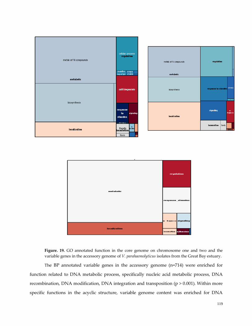
119

Figure. 19. GO annotated function in the core genome on chromosome one and two and the

variable genes in the accessory genome of V. parahaemolyticus isolates from the Great Bay estuary.

The BP annotated variable genes in the accessory genome (n=714) were enriched for

function related to DNA metabolic process, specifically nucleic acid metabolic process, DNA

recombination, DNA modification, DNA integration and transposition (p > 0.001). Within more

specific functions in the acyclic structure, variable genome content was enriched for DNA

120

alkylation, DNA methylation, defense response, clearance of foreign intracellular DNA, viral

process, life cycle, and virion assembly, symbiont process, multi-organism process, interspecies

interaction, O antigen biosynthetic process, O antigen metabolic process, response to stress and

cell adhesion (p > 0.001) (Figure 18). The variable content that was annotated with BP GO function

was mapped to the first or second chromosome (n=294) or were from isolates where their location

was not resolved (n=420). Both plasmids contained fewer than 10 BP GO annotated genes. Genes

for sporulation inhabitation, and chromosome partitioning were found on both. The larger

plasmid was annotated with genes related to DNA modification whereas the smaller plasmid

was annotated with two genes for antitoxin (chpS, higA-1) and a cold shock protein (cspG).

3.2 Local adaptation

The potential ecological relevance of the diversity of the isolates from the GBE was also

assessed in relationship to Vibrio parahaemolyticus collected from outside the GBE. The core

genome in the GBE (3,931 genes) consisted of approximately 1,677 more genes than the 2,254

genes cgMLST suggested by Gonzalez-Escalona et al., (2017). It is important to note that only 64

genes from the cgMLST were not present in in the GBE core genome and the majority of these

(52/64) were annotated as hypothetical proteins. The core content that was part of the cgMLST

was mapped to either the first (n= 1,563) or second chromosome (n=624) chromosome. Likewise,

the additional 1,677 genes in the GBE core genome were found on either the first (n= 923) or

second (n=722) chromosome (Figure 20). The V. parahaemolyticus cgMLST was significantly

enriched for genes involved with metabolism, specifically, organonitrogen compound metabolic

process and protein metabolic processes and translation and cell cycle processes (p > 0.001),

whereas the genes in the extra GBE core were enriched in functions related to localization, cell

projection organization, cellular response to stimulus, transport and signaling (p > 0.05). Further

work is needed to assess the biological validity of these differences based on the relatively low

number of genes assigned with GO terms. For example, if there were significantly more annotated

genes in the extra GBE core that mapped to the second chromosome and likewise more annotated

genes in the cgMLST core that mapped to the first chromosome, then that could account for the

differences in the functional enrichment between the cgMLST and the extra GBE core.

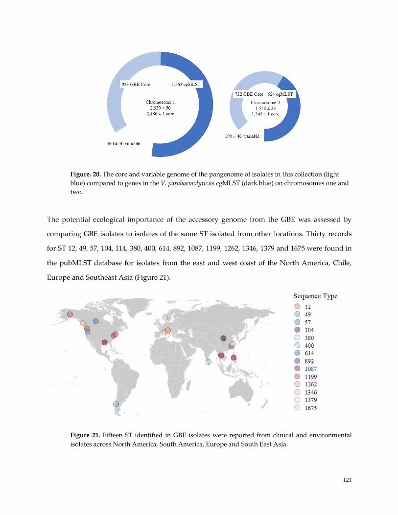
121

Figure. 20. The core and variable genome of the pangenome of isolates in this collection (light

blue) compared to genes in the V. parahaemolyticus cgMLST (dark blue) on chromosomes one and

two.

The potential ecological importance of the accessory genome from the GBE was assessed by

comparing GBE isolates to isolates of the same ST isolated from other locations. Thirty records

for ST 12, 49, 57, 104, 114, 380, 400, 614, 892, 1087, 1199, 1262, 1346, 1379 and 1675 were found in

the pubMLST database for isolates from the east and west coast of the North America, Chile,

Europe and Southeast Asia (Figure 21).

Figure 21. Fifteen ST identified in GBE isolates were reported from clinical and environmental

isolates across North America, South America, Europe and South East Asia.

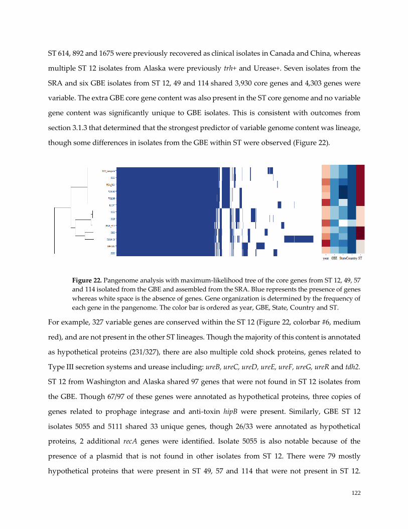
122

ST 614, 892 and 1675 were previously recovered as clinical isolates in Canada and China, whereas

multiple ST 12 isolates from Alaska were previously trh+ and Urease+. Seven isolates from the

SRA and six GBE isolates from ST 12, 49 and 114 shared 3,930 core genes and 4,303 genes were

variable. The extra GBE core gene content was also present in the ST core genome and no variable

gene content was significantly unique to GBE isolates. This is consistent with outcomes from

section 3.1.3 that determined that the strongest predictor of variable genome content was lineage,

though some differences in isolates from the GBE within ST were observed (Figure 22).

Figure 22. Pangenome analysis with maximum-likelihood tree of the core genes from ST 12, 49, 57

and 114 isolated from the GBE and assembled from the SRA. Blue represents the presence of genes

whereas white space is the absence of genes. Gene organization is determined by the frequency of

each gene in the pangenome. The color bar is ordered as year, GBE, State, Country and ST.

For example, 327 variable genes are conserved within the ST 12 (Figure 22, colorbar #6, medium

red), and are not present in the other ST lineages. Though the majority of this content is annotated

as hypothetical proteins (231/327), there are also multiple cold shock proteins, genes related to

Type III secretion systems and urease including: ureB, ureC, ureD, ureE, ureF, ureG, ureR and tdh2.

ST 12 from Washington and Alaska shared 97 genes that were not found in ST 12 isolates from

the GBE. Though 67/97 of these genes were annotated as hypothetical proteins, three copies of

genes related to prophage integrase and anti-toxin hipB were present. Similarly, GBE ST 12

isolates 5055 and 5111 shared 33 unique genes, though 26/33 were annotated as hypothetical

proteins, 2 additional recA genes were identified. Isolate 5055 is also notable because of the

presence of a plasmid that is not found in other isolates from ST 12. There were 79 mostly

hypothetical proteins that were present in ST 49, 57 and 114 that were not present in ST 12.

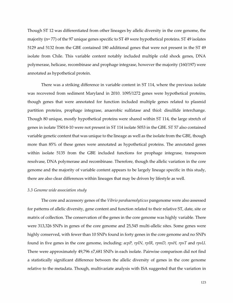
123

Though ST 12 was differentiated from other lineages by allelic diversity in the core genome, the

majority (n= 77) of the 97 unique genes specific to ST 49 were hypothetical proteins. ST 49 isolates

5129 and 5132 from the GBE contained 180 additional genes that were not present in the ST 49

isolate from Chile. This variable content notably included multiple cold shock genes, DNA

polymerase, helicase, recombinase and prophage integrase, however the majority (160/197) were

annotated as hypothetical protein.

There was a striking difference in variable content in ST 114, where the previous isolate

was recovered from sediment Maryland in 2010. 1095/1272 genes were hypothetical proteins,

though genes that were annotated for function included multiple genes related to plasmid

partition proteins, prophage integrase, anaerobic sulfatase and thiol: disulfide interchange.

Though 80 unique, mostly hypothetical proteins were shared within ST 114, the large stretch of

genes in isolate TS014-10 were not present in ST 114 isolate 5053 in the GBE. ST 57 also contained

variable genetic content that was unique to the lineage as well as the isolate from the GBE, though

more than 85% of these genes were annotated as hypothetical proteins. The annotated genes

within isolate 5135 from the GBE included functions for prophage integrase, transposon

resolvase, DNA polymerase and recombinase. Therefore, though the allelic variation in the core

genome and the majority of variable content appears to be largely lineage specific in this study,

there are also clear differences within lineages that may be driven by lifestyle as well.

3.3 Genome wide association study

The core and accessory genes of the Vibrio parahaemolyticus pangenome were also assessed

for patterns of allelic diversity, gene content and function related to their relative ST, date, site or

matrix of collection. The conservation of the genes in the core genome was highly variable. There

were 313,326 SNPs in genes of the core genome and 25,545 multi-allelic sites. Some genes were

highly conserved, with fewer than 10 SNPs found in forty genes in the core genome and no SNPs

found in five genes in the core genome, including: acpP, rpIN, rpIR, rpmD, rpsH, rpsT and rpsU.

There were approximately 49,796 ±7,681 SNPs in each isolate. Pairwise comparison did not find

a statistically significant difference between the allelic diversity of genes in the core genome

relative to the metadata. Though, multivariate analysis with ISA suggested that the variation in

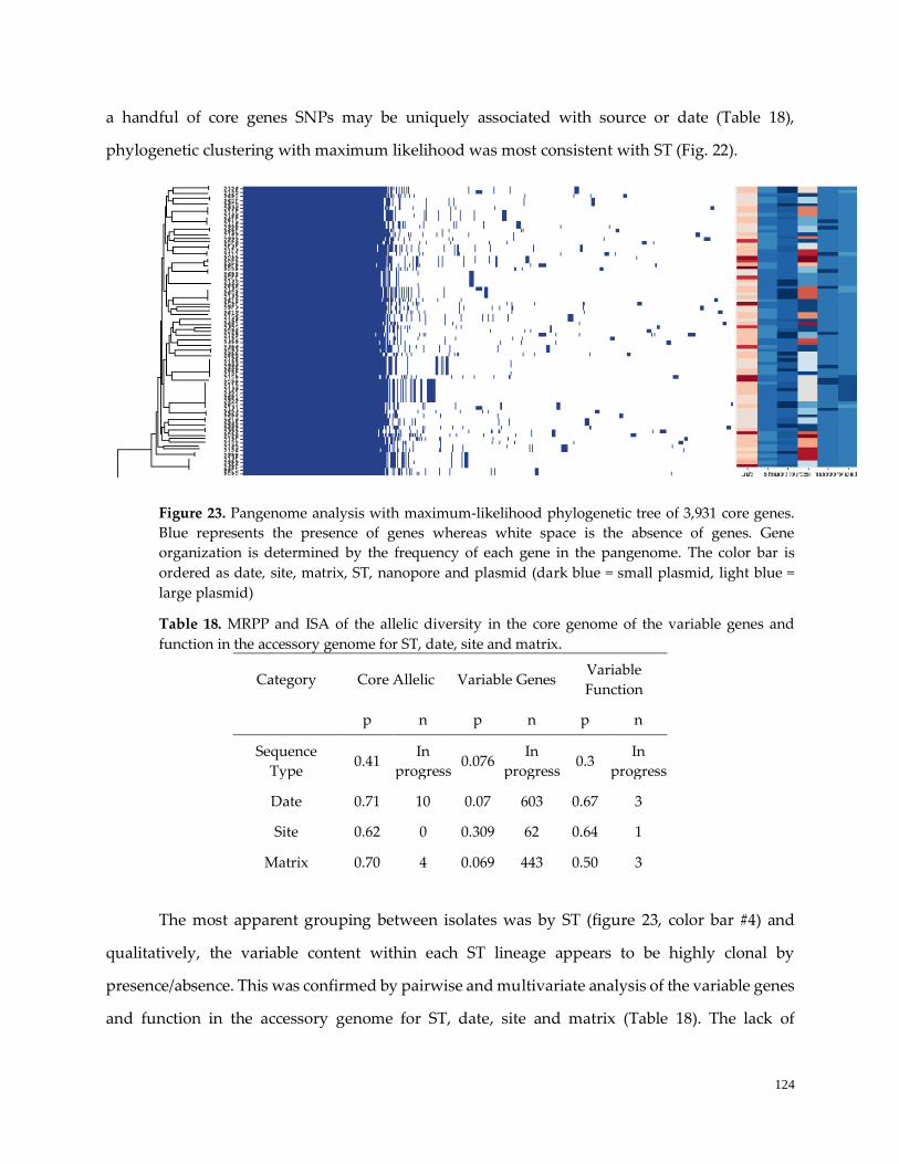
124

a handful of core genes SNPs may be uniquely associated with source or date (Table 18),

phylogenetic clustering with maximum likelihood was most consistent with ST (Fig. 22).

Figure 23. Pangenome analysis with maximum-likelihood phylogenetic tree of 3,931 core genes.

Blue represents the presence of genes whereas white space is the absence of genes. Gene

organization is determined by the frequency of each gene in the pangenome. The color bar is

ordered as date, site, matrix, ST, nanopore and plasmid (dark blue = small plasmid, light blue =

large plasmid)

Table 18. MRPP and ISA of the allelic diversity in the core genome of the variable genes and

function in the accessory genome for ST, date, site and matrix.

Category Core Allelic Variable Genes Variable

Function

p n p n p n

Sequence

Type 0.41

In

progress 0.076

In

progress 0.3

In

progress

Date 0.71 10 0.07 603 0.67 3

Site 0.62 0 0.309 62 0.64 1

Matrix 0.70 4 0.069 443 0.50 3

The most apparent grouping between isolates was by ST (figure 23, color bar #4) and

qualitatively, the variable content within each ST lineage appears to be highly clonal by

presence/absence. This was confirmed by pairwise and multivariate analysis of the variable genes

and function in the accessory genome for ST, date, site and matrix (Table 18). The lack of

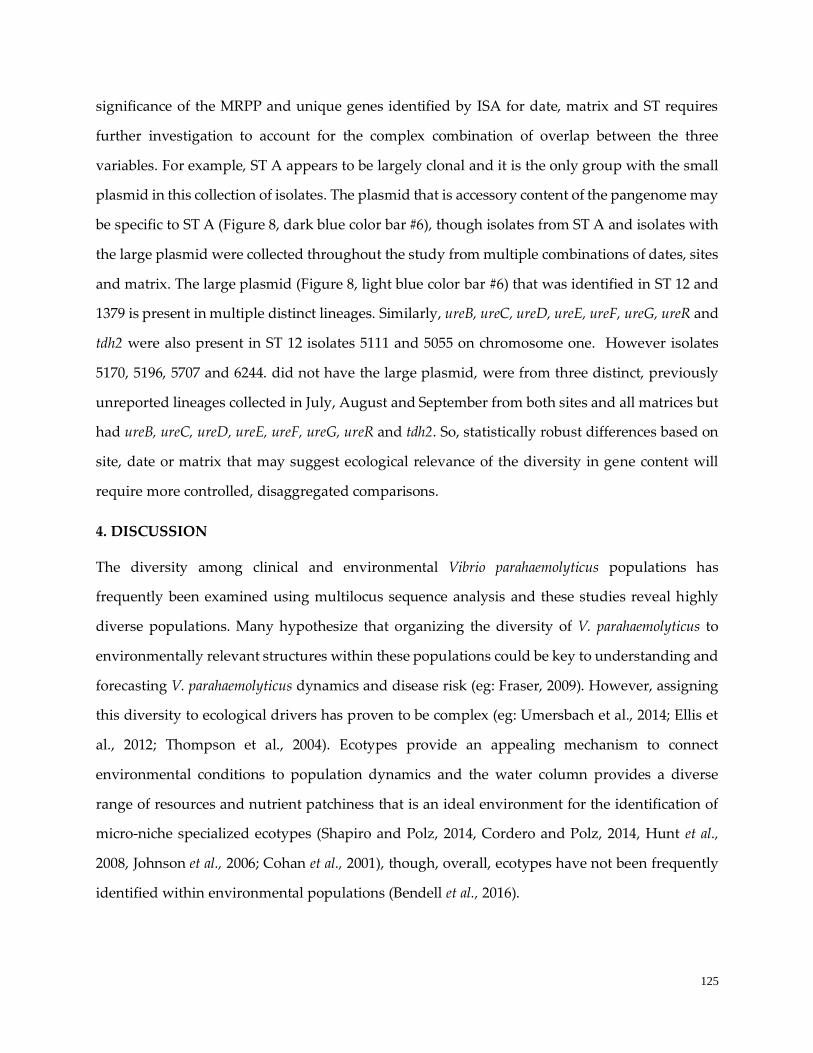
125

significance of the MRPP and unique genes identified by ISA for date, matrix and ST requires

further investigation to account for the complex combination of overlap between the three

variables. For example, ST A appears to be largely clonal and it is the only group with the small

plasmid in this collection of isolates. The plasmid that is accessory content of the pangenome may

be specific to ST A (Figure 8, dark blue color bar #6), though isolates from ST A and isolates with

the large plasmid were collected throughout the study from multiple combinations of dates, sites

and matrix. The large plasmid (Figure 8, light blue color bar #6) that was identified in ST 12 and

1379 is present in multiple distinct lineages. Similarly, ureB, ureC, ureD, ureE, ureF, ureG, ureR and

tdh2 were also present in ST 12 isolates 5111 and 5055 on chromosome one. However isolates

5170, 5196, 5707 and 6244. did not have the large plasmid, were from three distinct, previously

unreported lineages collected in July, August and September from both sites and all matrices but

had ureB, ureC, ureD, ureE, ureF, ureG, ureR and tdh2. So, statistically robust differences based on

site, date or matrix that may suggest ecological relevance of the diversity in gene content will

require more controlled, disaggregated comparisons.

4. DISCUSSION

The diversity among clinical and environmental Vibrio parahaemolyticus populations has

frequently been examined using multilocus sequence analysis and these studies reveal highly

diverse populations. Many hypothesize that organizing the diversity of V. parahaemolyticus to

environmentally relevant structures within these populations could be key to understanding and

forecasting V. parahaemolyticus dynamics and disease risk (eg: Fraser, 2009). However, assigning

this diversity to ecological drivers has proven to be complex (eg: Umersbach et al., 2014; Ellis et

al., 2012; Thompson et al., 2004). Ecotypes provide an appealing mechanism to connect

environmental conditions to population dynamics and the water column provides a diverse

range of resources and nutrient patchiness that is an ideal environment for the identification of

micro-niche specialized ecotypes (Shapiro and Polz, 2014, Cordero and Polz, 2014, Hunt et al.,

2008, Johnson et al., 2006; Cohan et al., 2001), though, overall, ecotypes have not been frequently

identified within environmental populations (Bendell et al., 2016).

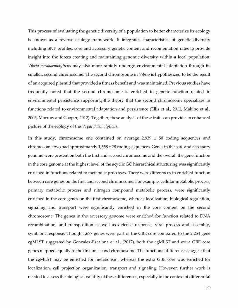
126

This process of evaluating the genetic diversity of a population to better characterize its ecology

is known as a reverse ecology framework. It integrates characteristics of genetic diversity

including SNP profiles, core and accessory genetic content and recombination rates to provide

insight into the forces creating and maintaining genomic diversity within a local population.

Vibrio parahaemolyticus may also more rapidly undergo environmental adaptation through its

smaller, second chromosome. The second chromosome in Vibrio is hypothesized to be the result

of an acquired plasmid that provided a fitness benefit and was maintained. Previous studies have

frequently noted that the second chromosome is enriched in genetic function related to

environmental persistence supporting the theory that the second chromosome specializes in

functions related to environmental adaptation and persistence (Ellis et al., 2012, Makino et al.,

2003, Morrow and Cooper, 2012). Together, these analysis of these traits can provide an enhanced

picture of the ecology of the V. parahaemolyticus.

In this study, chromosome one contained on average 2,939 ± 50 coding sequences and

chromosome two had approximately 1,558 ± 28 coding sequences. Genes in the core and accessory

genome were present on both the first and second chromosome and the overall the gene function

in the core genome at the highest level of the acyclic GO hierarchical structuring was significantly

enriched in functions related to metabolic processes. There were differences in enriched function

between core genes on the first and second chromosome. For example, cellular metabolic process,

primary metabolic process and nitrogen compound metabolic process, were significantly

enriched in the core genes on the first chromosome, whereas localization, biological regulation,

signaling and transport were significantly enriched in the core content on the second

chromosome. The genes in the accessory genome were enriched for function related to DNA

recombination, and transposition as well as defense response, viral process and assembly,

symbiont response. Though 1,677 genes were part of the GBE core compared to the 2,254 gene

cgMLST suggested by Gonzalez-Escalona et al., (2017), both the cgMLST and extra GBE core

genes mapped equally to the first or second chromosome. The functional differences suggest that

the cgMLST may be enriched for metabolism, whereas the extra GBE core was enriched for

localization, cell projection organization, transport and signaling. However, further work is

needed to assess the biological validity of these differences, especially in the context of differential

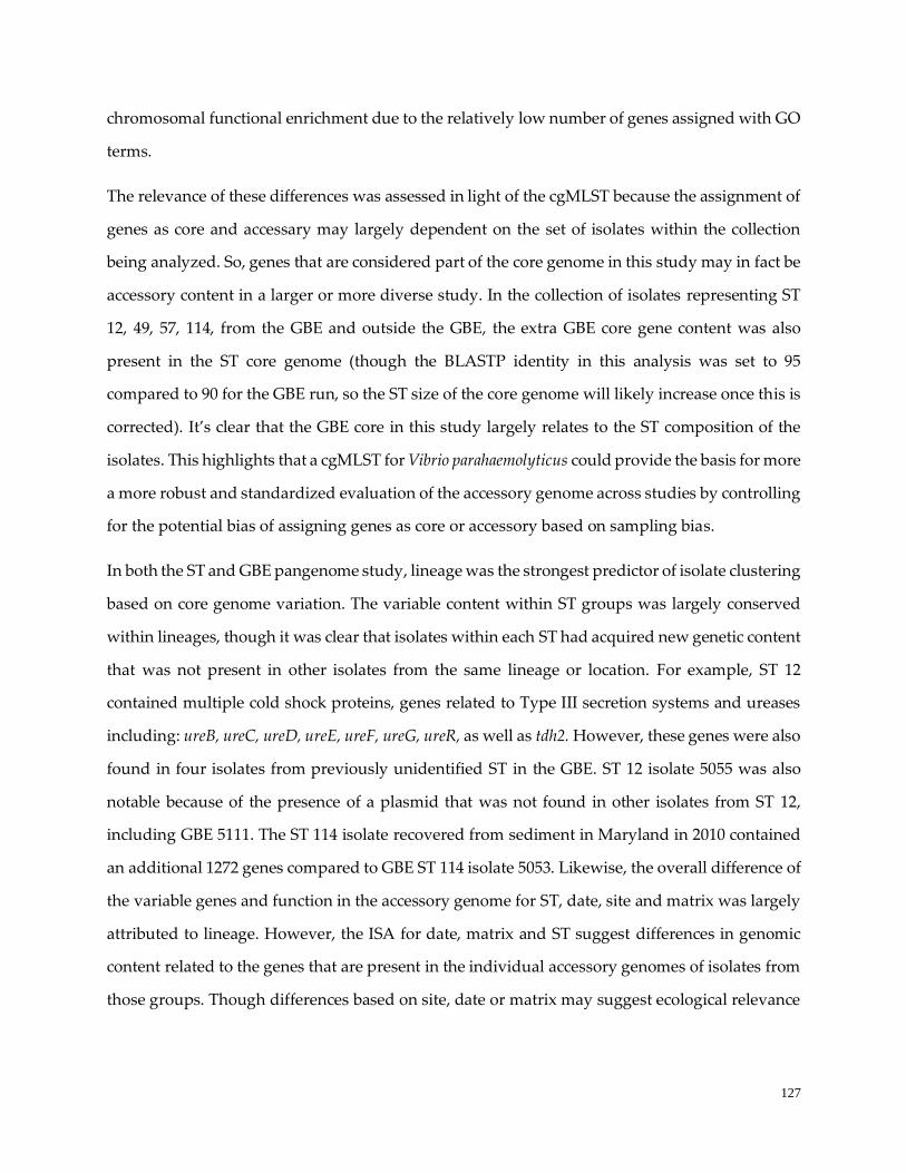
127

chromosomal functional enrichment due to the relatively low number of genes assigned with GO

terms.

The relevance of these differences was assessed in light of the cgMLST because the assignment of

genes as core and accessary may largely dependent on the set of isolates within the collection

being analyzed. So, genes that are considered part of the core genome in this study may in fact be

accessory content in a larger or more diverse study. In the collection of isolates representing ST

12, 49, 57, 114, from the GBE and outside the GBE, the extra GBE core gene content was also

present in the ST core genome (though the BLASTP identity in this analysis was set to 95

compared to 90 for the GBE run, so the ST size of the core genome will likely increase once this is

corrected). It’s clear that the GBE core in this study largely relates to the ST composition of the

isolates. This highlights that a cgMLST for Vibrio parahaemolyticus could provide the basis for more

a more robust and standardized evaluation of the accessory genome across studies by controlling

for the potential bias of assigning genes as core or accessory based on sampling bias.

In both the ST and GBE pangenome study, lineage was the strongest predictor of isolate clustering

based on core genome variation. The variable content within ST groups was largely conserved

within lineages, though it was clear that isolates within each ST had acquired new genetic content

that was not present in other isolates from the same lineage or location. For example, ST 12

contained multiple cold shock proteins, genes related to Type III secretion systems and ureases

including: ureB, ureC, ureD, ureE, ureF, ureG, ureR, as well as tdh2. However, these genes were also

found in four isolates from previously unidentified ST in the GBE. ST 12 isolate 5055 was also

notable because of the presence of a plasmid that was not found in other isolates from ST 12,

including GBE 5111. The ST 114 isolate recovered from sediment in Maryland in 2010 contained

an additional 1272 genes compared to GBE ST 114 isolate 5053. Likewise, the overall difference of

the variable genes and function in the accessory genome for ST, date, site and matrix was largely

attributed to lineage. However, the ISA for date, matrix and ST suggest differences in genomic

content related to the genes that are present in the individual accessory genomes of isolates from

those groups. Though differences based on site, date or matrix may suggest ecological relevance

128

of the diversity in gene content, this will require more controlled, disaggregated comparisons to

detect lifestyle driven differences within the overall influence of lineage.

The structure and content of the Vibrio parahaemolyticus genome is largely facilitated by variable

mutation rates coupled with combined with gene gain and loss. The overall content consists

predominantly of coding sequences (identified and hypothetical) with very little intragenic or

pseudogenic content (~5,000 orf and 5mb). Homologous recombination also provides the basis

for niche adaptation and diversification, for example the current genetic divergence within ST36

clonal population has been attributed to recombination (Martinez-Urtuza et al., 2017). Whereas

the most recognized mechanism for rapid niche adaptation in V. parahaemolyticus is homologous

recombination and horizontal gene transfer, Johnson et al., (2013) suggested that elevated

mutation rates may also facilitate niche adaptation. A current limitation of this study is the

emphasis on gene presence/absence and currently work is in process to more robustly assess the

allelic diversity of the pangenomes in this study, including analysis of recombination, selection

and linkage disequilibrium. This will also enable consideration of the majority of variable content

that is hypothetical proteins and not functionally annotated. Another potential direction that

needs to be considered is gene content that is orthologous at levels below 90% identity.

We show that the GBE Vibrio parahaemolyticus genomes are shaped by both lineage and the

environment, similar to findings by Tamames et al., (2016) and there is evidence of strains from

globally disparate regions remaining well-conserved and persisting over time. Though variable

content and allelic diversity are largely based on lineage in the GBE, there is also evidence of the

acquisition of novel genetic material that is integrated into the chromosome or present on

plasmids that are shared between distinct lineages consistent with findings by Bobay and

Ochman, (2017), Ceccarelli et al., (2013), Johnson, (2013) and Metzger and Blokesch, (2014).

The diversity within and between Vibrio parahaemolyticus populations has been proposed to arise

from the demands of the environment they inhabit. This idea of “niche sequestering” was

observed and reported by Johnson et al., (2012) in strains from the Gulf of Mexico and Shapiro

and Polz (2014) where V. parahaemolyticus strains from similar environmental niches were more

similar in genetic content and allelic diversity than they were to strains that were isolated from

129

different environmental conditions. Whereas both variable mutation rates across the genome and

horizontal gene transfer and have been shown to play a role in the evolution of V. parahaemolyticus

(Tamames et al., 2016), many believe that HGT and recombination is the predominant force

shaping the V. parahaemolyticus genome (Martinez-Urtaza et al., 2017; Ceccarelli et al., 2013;

Johnson et al., 2013).

Historically, phylogenetic assessment has been the most widely used epidemiological tool to trace

the evolutionary background or trajectory of the emergence of virulence within a population,

however, the ability of Vibrio parahaemolyticus to undergo recombination, even in conserved

regions believed to be limited to vertical acquisition, potentially masks many of the patterns

typically used to assess the development and succession of virulent lineages within largely non-

pathogenic populations. Given this, effective epidemiological reconstruction and investigation of

the mechanisms of pathogen evolution will require accounting for the many potential sources of

underlying diversity within populations. Environmentally relevant structure within these

populations could be key to understanding the diversity and drivers underlying community

dynamics and cycling in the estuarine environment. The relationship between genetic diversity

and the environment in the GBE remains to be clarified, however ecotype differentiation is an

important potential direction to better determining the basis for how environmental adaptation

shapes V. parahaemolyticus dynamics

130

References

Alexa A, Rahnenfuhrer J (2019). topGO: Enrichment Analysis for Gene Ontology. R package version

2.36.0.

Altschul, S.F., Gish, W., Miller, W., Myers, E.W. & Lipman, D.J. (1990) "Basic local alignment

search tool." J. Mol. Biol. 215:403-410

Andrew J. Page, Carla A. Cummins, Martin Hunt, Vanessa K. Wong, Sandra Reuter, Matthew T.

G. Holden, Maria Fookes, Daniel Falush, Jacqueline A. Keane, Julian Parkhill,

Bioinformatics, (2015). "Roary: Rapid large-scale prokaryote pan genome analysis", doi:

http://dx.doi.org/10.1093/bioinformatics/btv421

Andrews, S. (2010). FASTQC. A quality control tool for high throughput sequence data

Baker-Austin, C., Trinanes, J., Gonzalez-Escalona, N., & Martinez-Urtaza, J. (2017). Non-Cholera

Vibrios: The Microbial Barometer of Climate Change. Trends in Microbiology.

https://doi.org/10.1016/j.tim.2016.09.008

Bendall, M. L., Stevens, S. L. R., Chan, L. K., Malfatti, S., Schwientek, P., Tremblay, J.,

Malmstrom, R. R. (2016). Genome-wide selective sweeps and gene-specific sweeps in

natural bacterial populations. ISME Journal, 10(7), 1589–1601.


Blackwell, K. D., & Oliver, J. D. (2008). The ecology of Vibrio vulnificus, Vibrio cholerae, and Vibrio

parahaemolyticus in North Carolina estuaries. Journal of Microbiology (Seoul, Korea), 46(2),

146–153. https://doi.org/10.1007/s12275-007-0216-2

Bobay, L.-M., & Ochman, H. (2017). Biological Species Are Universal across Life’s Domains.

Genome Biology and Evolution, 9(3), 491–501. https://doi.org/10.1093/gbe/evx026

Bolger, A. M., Lohse, M., & Usadel, B. (2014). Trimmomatic: a flexible trimmer for Illumina

sequence data. Bioinformatics, 30(15), 2114-2120.

Brynildsrud O, Bohlin J, Scheffer L, Eldholm V. Rapid scoring of genes in microbial pan-

genome-wide association studies with Scoary. Genome Biol. 2016;17:238

Carlson M (2019). GO.db: A set of annotation maps describing the entire Gene Ontology. R package

version 3.8.2

Ceccarelli, D., Hasan, N. A., Huq, A., & Colwell, R. R. (2013). Distribution and dynamics of

epidemic and pandemic Vibrio parahaemolyticus virulence factors. Frontiers in Cellular and

Infection Microbiology, 3. https://doi.org/10.3389/fcimb.2013.00097

Centers for Disease Control and Prevention (CDC). (2013). Increase in Vibrio parahaemolyticus

illnesses associated with consumption of shellfish from several Atlantic coast harvest areas,

United States, 2013. Vibrio Illness (Vibriosis), 21.

Cohan, F. M. (2002). What are Bacterial Species? Annual Review of Microbiology, 56(1), 457–487.

http://dx.doi.org/10.1093/bioinformatics/btv421

131

https://doi.org/10.1146/annurev.micro.56.012302.160634

Cooper, V. S., Vohr, S. H., Wrocklage, S. C., & Hatcher, P. J. (2010). Why genes evolve faster on

secondary chromosomes in bacteria. PLoS Computational Biology.

https://doi.org/10.1371/journal.pcbi.1000732

Coordinators, N. R. (2016). Database resources of the national center for biotechnology

information. Nucleic acids research, 44(Database issue), D7.

Cordero, O. X., & Polz, M. F. (2014). Explaining microbial genomic diversity in light of

evolutionary ecology. Nature Reviews Microbiology. Nature Publishing Group.

https://doi.org/10.1038/nrmicro3218

Cui, Y., Yang, X., Didelot, X., Guo, C., Li, D., Yan, Y., Zhang, Y., Yuan, Y., Yang, H., Wang, J.

and Wang, J., 2015. Epidemic clones, oceanic gene pools, and eco-LD in the free living

marine pathogen Vibrio parahaemolyticus. Molecular biology and evolution, 32(6), pp.1396-

1410.

Danecek P, Auton A, Abecasis G, Albers CA, Banks E et al.Bioinformatics (Oxford, England)

2011;27;15;2156-8PUBMED: 21653522; PMC: 3137218; DOI: 10.1093/bioinformatics/btr33

Davey, M. E., & O’toole, G. A. (2000). Microbial Biofilms: from Ecology to Molecular Genetics.

Microbiology and Molecular Biology Reviews. https://doi.org/10.1128/MMBR.64.4.847-867.2000

Davis, B. J., Jacobs, J. M., Davis, M. F., Schwab, K. J., DePaola, A., & Curriero, F. C. (2017).

Environmental determinants of Vibrio parahaemolyticus in the Chesapeake Bay. Appl.

Environ. Microbiol., 83(21), e01147-17.

Davis, B. J., Jacobs, J. M., Zaitchik, B., DePaola, A., & Curriero, F. C. (2019). Vibrio

parahaemolyticus in the Chesapeake Bay: operational in situ prediction and forecast models

can benefit from inclusion of lagged water quality measurements. Applied and environmental

microbiology, 85(17), e01007-19.

De Caceres, M., Legendre, P. (2009). Associations between species and groups of sites: indices

and statistical inference. Ecology, URL http://sites.google.com/site/miqueldecaceres/

Deter, J., Solen, L., Antoine, V., Jaufrey, J., Annick, D., Dominique, H.H. (2010). Ecology of

pathogenic and non‐pathogenic Vibrio parahaemolyticus on the French Atlantic coast. Effects

of temperature, salinity, turbidity and chlorophyll a. Environmental microbiology, 12(4),

929-937.

Deepanjali, A., Kumar, H., Karunasagar, I., Karunasagar, I. Seasonal Variation in Abundance of

Total and Pathogenic Vibrio parahaemolyticus in Oysters along the Southwest Coast of India.

Applied and Environmental Microbiology. (2005) 71, 7.

http://aem.asm.org/content/71/7/3575.abstract

DePaola, A., Ulaszek, J., Kaysner, C. A., Tenge, B. J., Nordstrom, J. L., Wells, J., Gendel, S. M.

(2003). Molecular, serological, and virulence characteristics of Vibrio parahaemolyticus

isolated from environmental, food, and clinical sources in North America and Asia. Applied

132

and Environmental Microbiology. https://doi.org/10.1128/AEM.69.7.3999-4005.2003

DePaola, A.; Hopkins, L.H.; Peeler, J.T.; Wentz, B.; McPhearson, R.M. Incidence of Vibrio

parahaemolyticus in US coastal waters and oysters. Appl. Environ. Microbiol. 1990, 1;56(8),

2299-302.

Ellis, C. N., Schuster, B. M., Striplin, M. J., Jones, S. H., Whistler, C. A., & Cooper, V. S. (2012).

Influence of seasonality on the genetic diversity of Vibrio parahaemolyticus in New

Hampshire shellfish waters as determined by multilocus sequence analysis. Applied and

Environmental Microbiology. https://doi.org/10.1128/AEM.07794-11

Espejo, R. T., García, K., & Plaza, N. (2017, July 24). Insight into the origin and evolution of the

Vibrio parahaemolyticus pandemic strain. Frontiers in Microbiology. Frontiers Media S.A.


Emms, D. M., & Kelly, S. (2015). OrthoFinder: solving fundamental biases in whole genome

comparisons dramatically improves orthogroup inference accuracy. Genome biology,

16(1), 157.

Fraser, C., Alm, E. J., Polz, M. F., Spratt, B. G., & Hanage, W. P. (2009). The Bacterial Species

Challenge : Ecological Diversity. Science, 323(February), 741–746.

https://doi.org/10.1126/science.1159388

Friedman, J., Alm, E. J., & Shapiro, B. J. (2013). Sympatric Speciation: When Is It Possible in

Bacteria? PLoS ONE, 8(1). https://doi.org/10.1371/journal.pone.0053539

Froelich, B., Bowen, J., Gonzalez, R., Snedeker, A., & Noble, R. (2013). Mechanistic and statistical

models of total Vibrio abundance in the neuse river estuary. Water Research.

https://doi.org/10.1016/j.watres.2013.06.050

Froelich, B. A., & Noble, R. T. (2016). Vibrio bacteria in raw oysters: managing risks to human

health. Philosophical Transactions of the Royal Society B: Biological Sciences, 371(1689),

20150209.

Fujino, T., Okuno, Y., Nakada, D., Aoyama, A., Fukai, K., Mukai, T., & Ueho, T. (1953). On the

bacteriological examination of shirasu-food poisoning. Medical Journal of Osaka University,

4(2/3), 299-304.

Gilbert, J. A., Steele, J. A., Caporaso, J. G., Steinbrück, L., Reeder, J., Temperton, B., Field, D.

(2012). Defining seasonal marine microbial community dynamics. The ISME Journal.


Gonzalez-Escalona, N., Jolley, K. A., Reed, E., & Martinez-Urtaza, J. (2017). Defining a core

genome multilocus sequence typing scheme for the global epidemiology of Vibrio

parahaemolyticus. Journal of clinical microbiology, 55(6), 1682-1697.

Gurevich, A., Saveliev, V., Vyahhi, N., & Tesler, G. (2013). QUAST: quality assessment tool for

genome assemblies. Bioinformatics, 29(8), 1072-1075.

133

Hartwick, M., Berenson, A., Whistler, C.A., Cooper, V.S., and Jones, S.H. The Seasonal Ecology

of Vibrio parahaemolyticus and Plankton in a New Hampshire Estuary (in preparation)

Hartwick, M., Urquhart, A.E., Whistler, C.A., Cooper, V.S., Naumova, E.N., and Jones, S.H.

Forecasting Vibrio parahaemolyticus Concentration in Shellfish from a New England Estuary

(submitted)

Holden, M. T. G., Titball, R. W., Peacock, S. J., Cerdeño-Tárraga, A. M., Atkins, T., Crossman, L.

C., Parkhill, J. (2004). Genomic plasticity of the causative agent of melioidosis, Burkholderia

pseudomallei. Proceedings of the National Academy of Sciences of the United States of America,

101(39), 14240–14245. https://doi.org/10.1073/pnas.0403302101

Hunt, D. E., David, L. A., Gevers, D., Preheim, S. P., Alm, E. J., & Polz, M. F. (2008). Resource

partitioning and sympatric differentiation among closely related bacterioplankton. Science,

320(5879), 1081–1085. https://doi.org/10.1126/science.1157890

Inouye, M., Dashnow, H., Raven, L.A., Schultz, M.B., Pope, B.J., Tomita, T., Zobel, J. and Holt,

K.E., 2014. SRST2: rapid genomic surveillance for public health and hospital microbiology

labs. Genome medicine, 6(11), p.90.

Johnson, C. N. (2013). Fitness Factors in Vibrios: A Mini-review. Microbial Ecology, 65(4), 826–

851. https://doi.org/10.1007/s00248-012-0168-x

Jones, S.; Summer-Brason, B. Incidence and detection of pathogenic Vibrio spp. in a northern

New England estuary, USA. Journal of Shellfish Research 1998, 17, 1665–1669.

Kaneko and, T., & Colwell2, R. R. (1973). Ecology of Vibrio parahaemolyticus in Chesapeake Bay.

JOURNAL OF BACTERIOLOGY, 113(1), 24–32.

Kaneko, T., & Colwell, R. R. (1975). Incidence of Vibrio parahaemolyticus in Chesapeake Bay.


Katoh, K., & Standley, D. M. (2013). MAFFT multiple sequence alignment software version 7:

improvements in performance and usability. Molecular biology and evolution, 30(4), 772-780

Keymer, D. P., Miller, M. C., Schoolnik, G. K., & Boehm, A. B. (2007). Genomic and phenotypic

diversity of coastal Vibrio cholerae strains is linked to environmental factors. Appl. Environ.

Microbiol., 73(11), 3705-3714.

Leinonen, R., Sugawara, H., Shumway, M., & International Nucleotide Sequence Database

Collaboration. (2010). The sequence read archive. Nucleic acids research, 39(suppl_1), D19-

D21.

Le Roux, F., & Blokesch, M. (2018). Eco-evolutionary dynamics linked to horizontal gene

transfer in vibrios. Annual review of microbiology, 72, 89-110.

Li, Heng, Bob Handsaker, Alec Wysoker, Tim Fennell, Jue Ruan, Nils Homer, Gabor Marth,

Goncalo Abecasis, and Richard Durbin. The sequence alignment/map format and

SAMtools. Bioinformatics 25, no. 16 (2009): 2078-2079.

134

Lopez-Hernandez, K. M., Pardio-Sedas, V. T., Lizarraga-Partida, L., Williams, J. de J., Martinez-

Herrera, D., Flores-Primo, A., Rendon-Castro, K. (2015). Environmental parameters

influence on the dynamics of total and pathogenic Vibrio parahaemolyticus densities in

Crassostrea virginica harvested from Mexico’s Gulf coast. Marine Pollution Bulletin.

https://doi.org/10.1016/j.marpolbul.2014.11.015

Lovell, C. R. (2017). Ecological fitness and virulence features of Vibrio parahaemolyticus in

estuarine environments. Applied Microbiology and Biotechnology.

https://doi.org/10.1007/s00253-017-8096-9

Löytynoja, A. (2014). Phylogeny-aware alignment with PRANK. In Multiple sequence

alignment methods (pp. 155-170). Humana Press, Totowa, NJ.

Makino, K., Oshima, K., Kurokawa, K., Yokoyama, K., Uda, T., Tagomori, K., Iida, T. (2003).

Genome sequence of Vibrio parahaemolyticus: A pathogenic mechanism distinct from that of

V. cholerae. Lancet. https://doi.org/10.1016/S0140-6736(03)12659-1

Martinez-Urtaza, J., Baker-Austin, C., Jones, J. L., Newton, A. E., Gonzalez-Aviles, G. D., &

DePaola, A. (2013). Spread of Pacific Northwest Vibrio parahaemolyticus Strain. New England

Journal of Medicine. https://doi.org/10.1056/NEJMc1305535

Martinez-Urtaza, J., Blanco-Abad, V., Rodriguez-Castro, A., Ansede-Bermejo, J., Miranda, A., &

Rodriguez-Alvarez, M. X. (2012). Ecological determinants of the occurrence and dynamics

of Vibrio parahaemolyticus in offshore areas. The ISME Journal.


Martinez-Urtaza, J., Lozano-Leon, A., Varela-Pet, J., Trinanes, J., Pazos, Y., & Garcia-Martin, O.

(2008). Environmental determinants of the occurrence and distribution of Vibrio

parahaemolyticus in the rias of Galicia, Spain. Applied and Environmental Microbiology.

https://doi.org/10.1128/AEM.01307-07

Martinez-Urtaza, J., Van Aerle, R., Abanto, M., Haendiges, J., Myers, R. A., Trinanes, J.,

Gonzalez-Escalona, N. (2017). Genomic variation and evolution of Vibrio parahaemolyticus

ST36 over the course of a transcontinental epidemic expansion. MBio, 8(6).

https://doi.org/10.1128/mBio.01425-17

Meibom, K. L., Blokesch, M., Dolganov, N. A., Wu, C. Y., & Schoolnik, G. K. (2005).

Microbiology: Chitin induces natural competence in Vibrio cholerae. Science, 310(5755),

1824–1827. https://doi.org/10.1126/science.1120096

Metzger, L. C., & Blokesch, M. (2014). Composition of the DNA-uptake complex of Vibrio

cholerae. Mobile Genetic Elements, 4(1), e28142. https://doi.org/10.4161/mge.28142

Morrow, J. D., & Cooper, V. S. (2012). Evolutionary effects of translocations in bacterial

genomes. Genome Biology and Evolution. https://doi.org/10.1093/gbe/evs099

Nilsson, W. B., Paranjpye, R. N., Hamel, O. S., Hard, C., & Strom, M. S. (2019). Vibrio

parahaemolyticus risk assessment in the Pacific Northwest: it’s not what’s in the water.

135

FEMS Microbiology Ecology, 95(4). https://doi.org/10.1093/femsec/fiz027

Nurk, S., Bankevich, A., Antipov, D., Gurevich, A., Korobeynikov, A., Lapidus, A., Prjibelsky,

A., Pyshkin, A., Sirotkin, A., Sirotkin, Y. and Stepanauskas, R., 2013, April. Assembling

genomes and mini-metagenomes from highly chimeric reads. In Annual International

Conference on Research in Computational Molecular Biology (pp. 158-170). Springer,

Berlin, Heidelberg.

Oberbeckmann, S., Wichels, A., Wiltshire, K. H., & Gerdts, G. (2011). Occurrence of Vibrio

parahaemolyticus and Vibrio alginolyticus in the German Bight over a seasonal cycle.

Antonie van Leeuwenhoek, International Journal of General and Molecular Microbiology.

https://doi.org/10.1007/s10482-011-9586-x

Oberbeckmann, S., Fuchs, B. M., Meiners, M., Wichels, A., Wiltshire, K. H., & Gerdts, G. (2012).

Seasonal dynamics and modeling of a Vibrio community in coastal waters of the North Sea.

Microbial ecology, 63(3), 543-551.

Page, A.J., Taylor, B., Delaney, A.J., Soares, J., Seemann, T., Keane, J.A., Harris, S.R.,SNP-sites:

rapid efficient extraction of SNPs from multi-FASTA alignments", Microbial Genomics

2(4), (2016)

Panicker, G.; Call, D. R.; Krug, M. J.; Bej, A. K. Detection of pathogenic Vibrio spp. in shellfish by

using multiplex PCR and DNA microarrays. Applied and Environmental Microbiology

2004, 70(12), 7436–44.

Paranjpye, R., Hamel, O. S., Stojanovski, A., & Liermann, M. (2012). Genetic diversity of clinical

and environmental Vibrio parahaemolyticus strains from the Pacific northwest. Applied and

Environmental Microbiology, 78(24), 8631–8638. https://doi.org/10.1128/AEM.01531-12

Paranjpye, R. N., Nilsson, W. B., Liermann, M., Hilborn, E. D., George, B. J., Li, Q., Sandifer, P.

A. (2015). Environmental influences on the seasonal distribution of Vibrio parahaemolyticus

in the Pacific Northwest of the USA. FEMS Microbiology Ecology.

https://doi.org/10.1093/femsec/fiv121

Parveen, S., Hettiarachchi, K. A., Bowers, J. C., Jones, J. L., Tamplin, M. L., McKay, R., DePaola,

A. (2008). Seasonal distribution of total and pathogenic Vibrio parahaemolyticus in

Chesapeake Bay oysters and waters. International Journal of Food Microbiology, 128(2), 354–

361. https://doi.org/10.1016/j.ijfoodmicro.2008.09.019

Pedersen TL (2016). PanVizGenerator: Generate PanViz visualisations from your pangenome. R

package version 1.2.0, https://github.com/thomasp85/PanVizGenerator.

Pruzzo, C., Vezzulli, L., & Colwell, R. R. (2008, June). Global impact of Vibrio cholerae

interactions with chitin. Environmental Microbiology. https://doi.org/10.1111/j.1462-

2920.2007.01559.x

Quantitative Risk Assessment on the Public Health Impact of Pathogenic Vibrio parahaemolyticus

in Raw Oysters | FDA. (n.d.). Retrieved October 29, 2019, from

https://github.com/thomasp85/PanVizGenerator

136

https://www.fda.gov/food/cfsan-risk-safety-assessments/quantitative-risk-assessment-

public-health-impact-pathogenic-vibrio-parahaemolyticus-raw-oysters

R Core Team (2019). R: A language and environment for statistical computing. R Foundation for

Statistical Computing, Vienna, Austria. URL https://www.R-project.org/.

Semenza, J. C., Trinanes, J., Lohr, W., Sudre, B., Löfdahl, M., Martinez-Urtaza, J., Rocklöv, J.

(2017). Environmental suitability of Vibrio infections in a warming climate: An early

warning system. Environmental Health Perspectives, 125(10). https://doi.org/10.1289/EHP2198


cohesive units. Trends in Microbiology. https://doi.org/10.1016/j.tim.2014.02.006

Shinoda, S., & Miyoshi, S. ichi. (2006). Hemolysins of Vibrio cholerae and other Vibrio species. In

The Comprehensive Sourcebook of Bacterial Protein Toxins (pp. 748–762). Elsevier Inc.

https://doi.org/10.1016/B978-012088445-2/50049-4

Sun, F., Zhang, Y., Wang, L., Yan, X., Tan, Y., Guo, Z., Zhou, D. (2012). Molecular

Characterization of Direct Target Genes and cis-Acting Consensus Recognized by

Quorum-Sensing Regulator AphA in Vibrio parahaemolyticus. PLoS ONE, 7(9).


Takemura, A. F., Chien, D. M., & Polz, M. F. (2014). Associations and dynamics of Vibrionaceae

in the environment, from the genus to the population level. Frontiers in Microbiology.


Tamames, J., Sánchez, P. D., Nikel, P. I., & Pedrós-Alió, C. (2016). Quantifying the relative

importance of phylogeny and environmental preferences as drivers of gene content in

prokaryotic microorganisms. Frontiers in Microbiology, 7(MAR).


Thompson, J. R., Randa, M. A., Marcelino, L. A., Tomita-Mitchell, A., Lim, E., & Polz, M. F.

(2004). Diversity and dynamics of a North Atlantic coastal Vibrio community. Applied and

Environmental Microbiology. https://doi.org/10.1128/AEM.70.7.4103-4110.2004

Tonkin, J. D., Bogan, M. T., Bonada, N., Rios-Touma, B., & Lytle, D. A. (2017). Seasonality and

predictability shape temporal species diversity. Ecology, 98(5), 1201–1216.

https://doi.org/10.1002/ecy.1761

Turner, J. W., Berthiaume, C. T., Morales, R., Armbrust, E. V., & Strom, M. S. (2016). Genomic

evidence of adaptive evolution in emergent Vibrio parahaemolyticus ecotypes. Elementa:

Science of the Anthropocene. https://doi.org/10.12952/journal.elementa.000117

Turner, J. W., Malayil, L., Guadagnoli, D., Cole, D., & Lipp, E. K. (2014). Detection of Vibrio

parahaemolyticus, Vibrio vulnificus and Vibrio cholerae with respect to seasonal fluctuations in

temperature and plankton abundance. Environmental Microbiology.

https://doi.org/10.1111/1462-2920.12246

The UniProt Consortium. UniProt: a worldwide hub of protein knowledge. Nucleic Acids Res.

137

47: D506-515 (2019)

Seemann, T. (2014). Prokka: rapid prokaryotic genome annotation. Bioinformatics, 30(14), 2068-

2069.

Stamatakis, A. (2014). RAxML version 8: a tool for phylogenetic analysis and post-analysis of

large phylogenies. Bioinformatics, 30(9), 1312-1313.

Urmersbach, S., Alter, T., Koralage, M. S. G., Sperling, L., Gerdts, G., Messelhäusser, U., &

Huehn, S. (2014). Population analysis of Vibrio parahaemolyticus originating from different

geographical regions demonstrates a high genetic diversity. BMC Microbiology, 14, 59.

https://doi.org/10.1186/1471-2180-14-59

Urquhart, E. A., Jones, S. H., Yu, J. W., Schuster, B. M., Marcinkiewicz, A. L., Whistler, C. A., &

Cooper, V. S. (n.d.). Environmental Conditions Associated with Elevated Vibrio

parahaemolyticus Concentrations in Great Bay Estuary, New Hampshire.


Venkateswaran, K., Kiiyukia, C., Nakanishi, K., Nakano, H., Matsuda, O., & Hashimoto, H.

(1990). The role of sinking particles in the overwintering process of Vibrio parahaemolyticus

in a marine environment. FEMS Microbiology Ecology, 6(2), 159-166.

Vezzulli, L., Brettar, I., Pezzati, E., Reid, P. C., Colwell, R. R., Höfle, M. G., & Pruzzo, C. (2012).

Long-term effects of ocean warming on the prokaryotic community: evidence from the

vibrios. The ISME Journal. https://doi.org/10.1038/ismej.2011.89

Vezzulli, L., Pezzati, E., Moreno, M., Fabiano, M., Pane, L., Pruzzo, C., & The VibrioSea

Consortium. (2009). Benthic ecology of Vibrio spp. and pathogenic Vibrio species in a

coastal Mediterranean environment (La Spezia Gulf, Italy). Microbial Ecology.

https://doi.org/10.1007/s00248-009-9542-8

Weinert, L. A., & Welch, J. J. (2017, December 1). Why Might Bacterial Pathogens Have Small

Genomes? Trends in Ecology and Evolution. Elsevier Ltd.

https://doi.org/10.1016/j.tree.2017.09.006

Wick, R. R., Judd, L. M., Gorrie, C. L., & Holt, K. E. (2017). Unicycler: resolving bacterial genome

assemblies from short and long sequencing reads. PLoS computational biology, 13(6),

e1005595.

Wick, R. R., Schultz, M. B., Zobel, J., & Holt, K. E. (2015). Bandage: interactive visualization of de

novo genome assemblies. Bioinformatics, 31(20), 3350-3352.


environmental persistence and clinical nature of the human pathogen Vibrio vulnificus.


Xu, F., Gonzalez-Escalona, N., Haendiges, J., Myers, R. A., Ferguson, J., Stiles, T., Whistler, C. A.

(2017). Sequence type 631 Vibrio parahaemolyticus, an emerging foodborne pathogen in

North America. Journal of Clinical Microbiology. https://doi.org/10.1128/JCM.02162-16

138

Xu, F., Ilyas, S., Hall, J. A., Jones, S. H., Cooper, V. S., & Whistler, C. A. (2015). Genetic

characterization of clinical and environmental Vibrio parahaemolyticus from the Northeast

USA reveals emerging resident and non-indigenous pathogen lineages. Frontiers in

Microbiology. https://doi.org/10.3389/fmicb.2015.00272

Yang, C., Pei, X., Wu, Y., Yan, L., Yan, Y., Song, Y., Coyle, N.M., Martinez-Urtaza, J., Quince, C.,

Hu, Q. and Jiang, M., 2019. Recent mixing of Vibrio parahaemolyticus populations. The ISME

Journal, p.1.

Young, I., Gropp, K., Fazil, A., & Smith, B. A. (2015). Knowledge synthesis to support risk

assessment of climate change impacts on food and water safety: A case study of the effects

of water temperature and salinity on Vibrio parahaemolyticus in raw oysters and harvest

waters. Food Research International, 68, 86-93.

Yu G, Smith D, Zhu H, Guan Y, Lam TT (2017). ggtree: an R package for visualization and

annotation of phylogenetic trees with their covariates and other associated data. Methods in

Ecology and Evolution, 8, 28-36. doi: 10.1111/2041-210X.12628,

http://onlinelibrary.wiley.com/doi/10.1111/2041-210X.12628/abstract

Zimmerman, A. M., DePaola, A., Bowers, J. C., Krantz, J. A., Nordstrom, J. L., Johnson, C. N., &

Grimes, D. J. (2007). Variability of total and pathogenic Vibrio parahaemolyticus densities in

Northern Gulf of Mexico water and oysters. Applied and Environmental Microbiology.

https://doi.org/10.1128/AEM.01700-07

http://onlinelibrary.wiley.com/doi/10.1111/2041-210X.12628/abstract

FORECASTING VIBRIO PARAHAEMOLYTICUS IN A ... - CORE

Documents