1 Final Results of Assembly Line Balancing Problem Waldemar Grzechca The Silesian University of Technology Poland 1. Introduction The manufacturing assembly line was first introduced by Henry Ford in the early 1900’s. It was designed to be an efficient, highly productive way of manufacturing a particular product. The basic assembly line consists of a set of workstations arranged in a linear fashion, with each station connected by a material handling device. The basic movement of material through an assembly line begins with a part being fed into the first station at a predetermined feed rate. A station is considered any point on the assembly line in which a task is performed on the part. These tasks can be performed by machinery, robots, and/or human operators. Once the part enters a station, a task is then performed on the part, and the part is fed to the next operation. The time it takes to complete a task at each operation is known as the process time (Sury, 1971). The cycle time of an assembly line is predetermined by a desired production rate. This production rate is set so that the desired amount of end product is produced within a certain time period (Baybars, 1986). In order for the assembly line to maintain a certain production rate, the sum of the processing times at each station must not exceed the stations’ cycle time (Fonseca et al, 2005). If the sum of the processing times within a station is less than the cycle time, idle time is said to be present at that station (Erel et al,1998). One of the main issues concerning the development of an assembly line is how to arrange the tasks to be performed. This arrangement may be somewhat subjective, but has to be dictated by implied rules set forth by the production sequence (Kao, 1976). For the manufacturing of any item, there are some sequences of tasks that must be followed. The assembly line balancing problem (ALBP) originated with the invention of the assembly line. Helgeson et al (Helgeson et al, 1961) were the first to propose the ALBP, and Salveson (Salveson, 1955) was the first to publish the problem in its mathematical form. However, during the first forty years of the assembly line’s existence, only trial-and-error methods were used to balance the lines (Erel et al,, 1998). Since then, there have been numerous methods developed to solve the different forms of the ALBP. Salveson (Salveson, 1955) provided the first mathematical attempt by solving the problem as a linear program. Gutjahr and Nemhauser (Gutjahr & Nemhauser, 1964) showed that the ALBP problem falls into the class of NP-hard combinatorial optimization problems. This means that an optimal solution is not guaranteed for problems of significant size. Therefore, heuristic methods have become the most popular techniques for solving the problem. www.intechopen.com

Welcome message from author
This document is posted to help you gain knowledge. Please leave a comment to let me know what you think about it! Share it to your friends and learn new things together.
Transcript
1
Final Results of Assembly Line Balancing Problem
Waldemar Grzechca The Silesian University of Technology
Poland
1. Introduction
The manufacturing assembly line was first introduced by Henry Ford in the early 1900’s.
It was designed to be an efficient, highly productive way of manufacturing a particular
product. The basic assembly line consists of a set of workstations arranged in a linear
fashion, with each station connected by a material handling device. The basic movement
of material through an assembly line begins with a part being fed into the first station at a
predetermined feed rate. A station is considered any point on the assembly line in which a
task is performed on the part. These tasks can be performed by machinery, robots, and/or
human operators. Once the part enters a station, a task is then performed on the part, and
the part is fed to the next operation. The time it takes to complete a task at each operation
is known as the process time (Sury, 1971). The cycle time of an assembly line is
predetermined by a desired production rate. This production rate is set so that the desired
amount of end product is produced within a certain time period (Baybars, 1986). In order
for the assembly line to maintain a certain production rate, the sum of the processing
times at each station must not exceed the stations’ cycle time (Fonseca et al, 2005). If the
sum of the processing times within a station is less than the cycle time, idle time is said to
be present at that station (Erel et al,1998). One of the main issues concerning the
development of an assembly line is how to arrange the tasks to be performed. This
arrangement may be somewhat subjective, but has to be dictated by implied rules set
forth by the production sequence (Kao, 1976). For the manufacturing of any item, there
are some sequences of tasks that must be followed. The assembly line balancing problem
(ALBP) originated with the invention of the assembly line. Helgeson et al (Helgeson et al,
1961) were the first to propose the ALBP, and Salveson (Salveson, 1955) was the first to
publish the problem in its mathematical form. However, during the first forty years of the
assembly line’s existence, only trial-and-error methods were used to balance the lines
(Erel et al,, 1998). Since then, there have been numerous methods developed to solve the
different forms of the ALBP. Salveson (Salveson, 1955) provided the first mathematical
attempt by solving the problem as a linear program. Gutjahr and Nemhauser (Gutjahr &
Nemhauser, 1964) showed that the ALBP problem falls into the class of NP-hard
combinatorial optimization problems. This means that an optimal solution is not
guaranteed for problems of significant size. Therefore, heuristic methods have become the
most popular techniques for solving the problem.
www.intechopen.com

Assembly Line – Theory and Practice
4
2. Heuristic methods in assembly line balancing problem
The heuristic approach bases on logic and common sense rather than on mathematical proof. Heuristics do not guarantee an optimal solution, but results in good feasible solutions which approach the true optimum. Most of the described heuristic solutions in literature are the ones designed for solving Single Assembly Line Balancing Problem. Moreover, most of them are based on simple priority rules (constructive methods) and generate one or a few feasible solutions. Task-oriented procedures choose the highest priority task from the list of available tasks and assign it to the earliest station which is assignable. Among task-oriented procedures we can distinguish immediate-update-first-fit (IUFF) and general-first-fit methods depending on whether the set of available tasks is updated immediately after assigning a task or after the assigning of all currently available tasks. Due to its greater flexibility immediate-update-first-fit method is used more frequently. The main idea behind this heuristic is assigning tasks to stations basing on the numerical score. There are several ways to determine (calculate) the score for each tasks. One could easily create his own way of determining the score, but it is not obvious if it yields good result. In the following section five different methods found in the literature are presented along with the solution they give for our simple example. The methods are implemented in the Line Balancing program as well. From the moment the appropriate score for each task is determined there is no difference in execution of methods and the required steps to obtain the solution are as follows: Step 1. Assign a numerical score n(x) to each task x. Step 2. Update the set of available tasks (those whose immediate predecessors have been
already assigned). Step 3. Among the available tasks, assign the task with the highest numerical score to the
first station in which the capacity and precedence constraints will not be violated. Go to STEP 2.
The most popular heuristics which belongs to IUFF group are: IUFF-RPW Immediate Update First Fit – Ranked Positional Weight, IUFF-NOF Immediate Update First Fit – Number of Followers, IUFF-NOIF Immediate Update First Fit – Number of Immediate Followers, IUFF-NOP Immediate Update First Fit – Number of Predecessors, IUFF-WET Immediate Update First Fit – Work Element Time. In the literature we can often find the implementation of Kilbridge & Wester or Moodie & Young methods, too. Both of them base on precedence graph or precedence matrix of produced items.
3. Measures of final results of assembly line balancing problem
Some measures of solution quality have appeared in line balancing problem. Below are presented three of them (Scholl, 1999). Line efficiency (LE) shows the percentage utilization of the line. It is expressed as ratio of total station time to the cycle time multiplied by the number of workstations:
K
ii 1
ST
LE 100%c K== ⋅
⋅
(1)
where: K - total number of workstations, c - cycle time.
www.intechopen.com

Final Results of Assembly Line Balancing Problem
5
Smoothness index (SI) describes relative smoothness for a given assembly line balance. Perfect balance is indicated by smoothness index 0. This index is calculated in the following manner:
( )K
2max i
i 1
SI ST ST=
= − (2)
where: STmax - maximum station time (in most cases cycle time), STi - station time of station i. Time of the line (LT) describes the period of time which is need for the product to be completed on an assembly line:
( ) KLT c K 1 T= ⋅ − + (3)
where: c - cycle time, K -total number of workstations, TK – processing time of last station. Two-sided assembly lines (Fig. 1.) are typically found in producing large-sized products, such as trucks and buses. Assembling these products is in some respects different from assembling small products. Some assembly operations prefer to be performed at one of the two sides (Bartholdi, 1993).
Station n
Conveyor
Station 1 Station 3
Station (n-2) Station 4 Station 2
Station (n-3) Station (n-1)
Fig. 1. Two-sided assembly line structure
The final result estimation of two-sided assembly line balance needs some modification of existing measures (Grzechca, 2008). Time of line for TALBP
( ) { }K K 1LT c Km 1 Max t(S ) ,t(S )−= ⋅ − + (4)
where: Km – number of mated-stations K – number of assigned single stations t(SK) – processing time of the last single station As far as smoothness index and line efficiency are concerned, its estimation, on contrary to LT, is performed without any change to original version. These criterions simply refer to each individual station, despite of parallel character of the method.
www.intechopen.com

Assembly Line – Theory and Practice
6
But for more detailed information about the balance of right or left side of the assembly line additional measures will be proposed: Smoothness index of the left side
( )K
2L maxL iL
i 1
SI ST ST=
= − (5)
where: SIL- smoothness index of the left side of two-sided line STmaxL- maximum of duration time of left allocated stations STiL- duration time of i-th left allocated station Smoothness index of the right side
( )K
2R maxR iR
i 1
SI ST ST=
= − (6)
where:
SIR- smoothness index of the right side of two-sided line,
STmaxR- maximum of duration time of right allocated stations,
STiR- duration time of i-th right allocated station.
4. Line and station efficiency
Efficiency line was introduced to the assembly line balancing problem by Salveson. It was
the optimization goal of ALBP and the best solution was when it achieved 100%.
Unfortunately this measure is only useful when number of stations or cycle time are
changed. If for many final results we obtain the same number of stations and cycle time the
line efficiency does not deliver us the detailed knowledge about quality of the line balance.
Example of 12 tasks will be discussed. In Table 1 processing task times are presented. Figure
2 shows the relations between tasks (technology of assembly).
Fig. 2. Precedence graph of 12 tasks numerical example
www.intechopen.com
Final Results of Assembly Line Balancing Problem
7
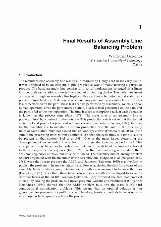
task 1 2 3 4 5 6 7 8 9 10 11 12
time 20 40 70 10 30 11 32 60 27 38 50 12
Table 1. Operation times for numerical example
Ranked Positional Weight (Halgeson et al, 1961) and Immediate Update First Fit – Working Element Time heuristics for obtaining the balance of assembly line were chosen. As we can see ( Fig. 3 ÷ 5) final results are different. For time-oriented balance we got 5 stations and LE for different heuristics is the same. Author proposes an additional station efficiency measurement which allows to find “bottleneck” in the production system and helps to estimate a good feasible line balance. The new measure describes more detailed the efficiency of each workstation and helps to find the worst point in whole assembly structure. Station efficiency (LESTi) shows the percentage utilization of each workstation. It is expressed as ratio of station time to the cycle time:
iSTi
STLE 100%
c= ⋅ (7)
Measures RPW
heuristic IUFF–WET
heuristic Measures
RPW heuristic
IUFF–WET heuristic
SI 40,42 59,08 LEST1 90 % 81 %
LT 462 462 LEST1 92 % 98 %
LE 80% 80% LEST1 65 % 59 %
LEST1 90 % 100 % LEST1 62 % 62 %
Table 2. Detailed measures of final results of RPW and IUFF-WET heuristics
Fig. 3. Final balance of 12 tasks example using RPW heuristic
www.intechopen.com
Assembly Line – Theory and Practice
8
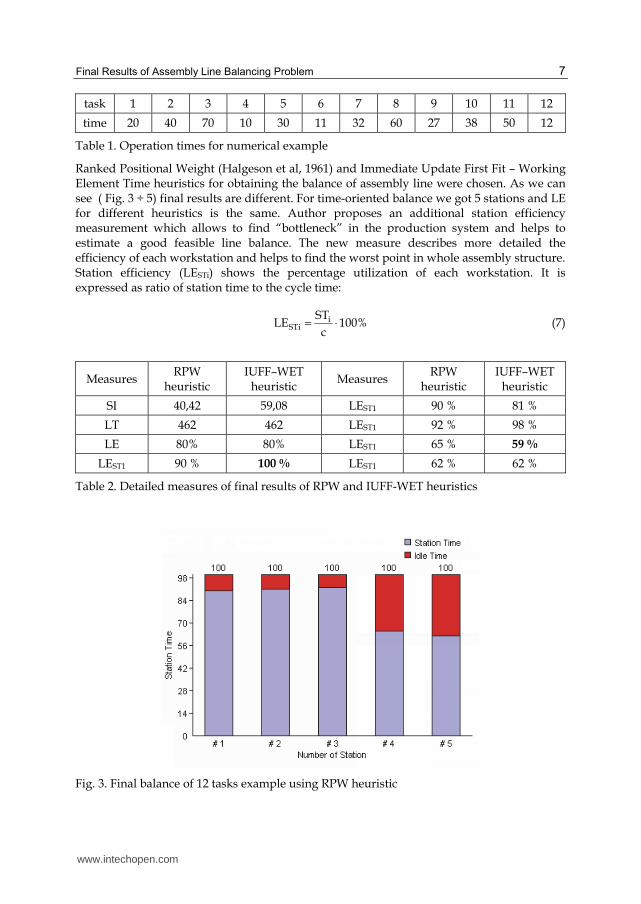
Fig. 4. Final balance of 12 tasks example using IUFF-WET heuristic
RPW HEURISTIC IUFF – WET HEURISTIC
Fig. 5. Station efficiency of 12 tasks example using RPW and IUFF – WET heuristics
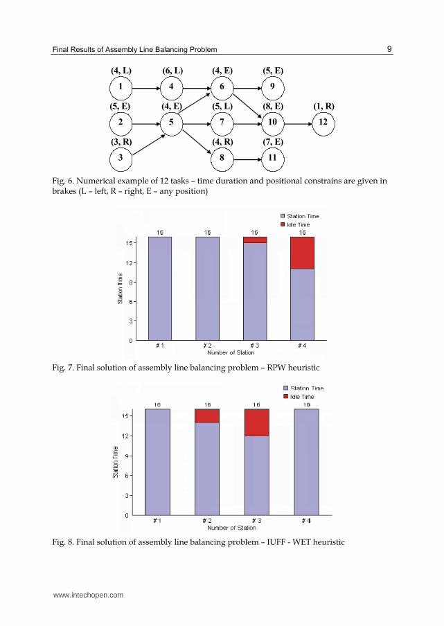
5. Last station problem
Below are presented two heuristic solution. We consider the case of single assembly line
(Fig. 6.) where all tasks can be assigned to any position (E). The cycle time is 16.
Fig. 7. presents solution where three stations have efficiency 100 % or very close to the value.
Last station has an idle time which is a consequence of completed number of tasks. Fig. 8.
shows solution where the last station is utilized in 100 %. The contribution of tasks causes
idle times of second and third station. As we can observe both solutions are feasible but with
different assignment of tasks and different station efficiency. RPW solution is near optimal
but the last station idle time is the biggest of all stations. WET solution is feasible and not so
close to optimal but smoothness index of this final result is smaller (balancing or equalizing
problem).
www.intechopen.com
Final Results of Assembly Line Balancing Problem
9
1
4
5
2
3
6
7
8
9
10
11
12
(4, L)
(5, E)
(3, R)
(6, L)
(4, E)
(4, R)
(5, L)
(4, E) (5, E)
(8, E)
(7, E)
(1, R)
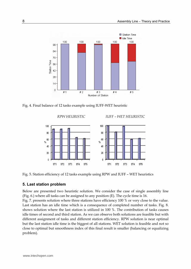
Fig. 6. Numerical example of 12 tasks – time duration and positional constrains are given in brakes (L – left, R – right, E – any position)
Fig. 7. Final solution of assembly line balancing problem – RPW heuristic
Fig. 8. Final solution of assembly line balancing problem – IUFF - WET heuristic
www.intechopen.com

Assembly Line – Theory and Practice
10
6. Assembly line structure problem
We consider numerical example from Fig. 8. The positional constrains are respected. As we can observe not only assigning of task becomes a problem (Fig. 9. ÷ Fig. 14.). The structure of assembly line can changed for different cycle times (Grzechca, 2010).
Fig. 9. Assembly line balance (c=16)
Fig. 10. Assembly line structure (c=16)
Fig. 11. Assembly line balance (c=15)
Station 1 Station 3
Station 2 Station4
Conveyour
www.intechopen.com

Final Results of Assembly Line Balancing Problem
11
Fig. 12. Assembly line structure (c=15)
Fig. 13. Assembly line balance (c=12)
Fig. 14. Assembly line structure (c=12)
In two-sided assembly line balancing problem it is very difficult to obtain a complete station
structure. This type of line very hard depends on precedence and position constraints.
Station 5
Station 4
Station 3
Station 2
Station 1
Conveyour
Station 6
S ta tio n 1
S ta tio n 8
S ta tio n 7
S ta tio n 6
S ta tio n 5
S ta tio n 4
S ta tio n 3
S ta tio n 2
1 4
2 3 5
6 9
8 1 1
7
1 0 1 2
C = 1 2
Station 1 Station 3 Station 5 Station 7
Station 2 Station 4 Station 6 Station 8
Conveyour
www.intechopen.com

Assembly Line – Theory and Practice
12
7. Conclusions
Assembly lines are a popular manufacturing structure. Assembly line balancing problem is known more than 50 years. There are hundreds exact and heuristic methods. It is very important to obtain the feasible and acceptable results. It is very important to analyze and estimate the final results and to implement the best one. Author of the chapter hopes that the presented knowledge helps to understand the problem.
8. References
Bartholdi, J.J. (1993). Balancing two-sided assembly lines: A case study, International Journal of Production Research, Vol. 31, No,10, pp. 2447-2461
Baybars, I. (1986). A survey of exact algorithms for simple assembly line balancing problem, Management Science, Vol. 32, No. 8, pp. 909-932
Erel, E., Sarin S.C. (1998). A survey of the assembly line balancing procedures, Production Planning and Control, Vol. 9, No. 5, pp. 414-434
Fonseca D.J., Guest C.L., Elam M., Karr C.L. (2005). A fuzzy logic approach to assembly line balancing, Mathware & Soft Computing, Vol. 12, pp. 57-74
Grzechca W. (2008) Two-sided assembly line. Estimation of final results. Proceedings of the Fifth International Conference on Informatics in Control, Automation and Robotics ICINCO 2008, Final book of Abstracts and Proceedings, Funchal, 11-15 May 2008, pp. 87-88, CD Version ISBN: 978-989-8111-35-7
Grzechca W. (2010) Structure’s Uncertainty of Two-sided Assembly Line Balancing Problem. URPDM 2010 Coimbra, CD version
Gutjahr, A.L., Neumhauser G.L. (1964). An algorithm for the balancing problem, Management Science, Vol. 11,No. 2, pp. 308-315
Helgeson W. B., Birnie D. P. (1961). Assembly line balancing using the ranked positional weighting technique, Journal of Industrial Engineering, Vol. 12, pp. 394-398
Kao, E.P.C. (1976). A preference order dynamic program for stochastic assembly line balancing, Management Science, Vol. 22, No. 10, pp. 1097-1104
Lee, T.O., Kim Y., Kim Y.K. (2001). Two-sided assembly line balancing to maximize work relatedness and slackness, Computers & Industrial Engineering, Vol. 40, No. 3, pp. 273-292
Salveson, M.E. (1955). The assembly line balancing problem, Journal of Industrial Engineering, Vol.6, No. 3. pp. 18-25
Scholl, A. (1999). Balancing and sequencing of assembly line, Physica- Verlag, ISBN 9783790811803, Heidelberg New-York
Sury, R.J. (1971). Aspects of assembly line balancing, International Journal of Production Research, Vol. 9, pp. 8-14
www.intechopen.com
Assembly Line - Theory and PracticeEdited by Prof. Waldemar Grzechca
ISBN 978-953-307-995-0Hard cover, 250 pagesPublisher InTechPublished online 17, August, 2011Published in print edition August, 2011
InTech EuropeUniversity Campus STeP Ri Slavka Krautzeka 83/A 51000 Rijeka, Croatia Phone: +385 (51) 770 447 Fax: +385 (51) 686 166www.intechopen.com
InTech ChinaUnit 405, Office Block, Hotel Equatorial Shanghai No.65, Yan An Road (West), Shanghai, 200040, China
Phone: +86-21-62489820 Fax: +86-21-62489821
An assembly line is a manufacturing process in which parts are added to a product in a sequential mannerusing optimally planned logistics to create a finished product in the fastest possible way. It is a flow-orientedproduction system where the productive units performing the operations, referred to as stations, are aligned ina serial manner. The present edited book is a collection of 12 chapters written by experts and well-knownprofessionals of the field. The volume is organized in three parts according to the last research works inassembly line subject. The first part of the book is devoted to the assembly line balancing problem. It includeschapters dealing with different problems of ALBP. In the second part of the book some optimization problemsin assembly line structure are considered. In many situations there are several contradictory goals that have tobe satisfied simultaneously. The third part of the book deals with testing problems in assembly line. Thissection gives an overview on new trends, techniques and methodologies for testing the quality of a product atthe end of the assembling line.
How to referenceIn order to correctly reference this scholarly work, feel free to copy and paste the following:
Waldemar Grzechca (2011). Final Results of Assembly Line Balancing Problem, Assembly Line - Theory andPractice, Prof. Waldemar Grzechca (Ed.), ISBN: 978-953-307-995-0, InTech, Available from:http://www.intechopen.com/books/assembly-line-theory-and-practice/final-results-of-assembly-line-balancing-problem

© 2011 The Author(s). Licensee IntechOpen. This chapter is distributedunder the terms of the Creative Commons Attribution-NonCommercial-ShareAlike-3.0 License, which permits use, distribution and reproduction fornon-commercial purposes, provided the original is properly cited andderivative works building on this content are distributed under the samelicense.
Related Documents


![Assembly Line Balancing Procedure - MDPI · 2020. 7. 20. · assembly line balancing (ALB) is the simple assembly line balancing (SALB) [13]. Besides other assumptions listed in [14],](https://static.cupdf.com/doc/110x72/6134dbe2dfd10f4dd73c001c/assembly-line-balancing-procedure-mdpi-2020-7-20-assembly-line-balancing.jpg)