THE MULTIPLE VEHICLE BALANCING PROBLEM

THE MULTIPLE VEHICLE BALANCING PROBLEM

Marco Casazza, Alberto Ceselli, Daniel Chemla, Frederic Meunier, Roberto

Wolfler Calvo

To cite this version:

Marco Casazza, Alberto Ceselli, Daniel Chemla, Frederic Meunier, Roberto Wolfler Calvo.THE MULTIPLE VEHICLE BALANCING PROBLEM. 2016. <hal-01351215>

HAL Id: hal-01351215

https://hal.archives-ouvertes.fr/hal-01351215

Submitted on 2 Aug 2016

HAL is a multi-disciplinary open accessarchive for the deposit and dissemination of sci-entific research documents, whether they are pub-lished or not. The documents may come fromteaching and research institutions in France orabroad, or from public or private research centers.

L’archive ouverte pluridisciplinaire HAL, estdestinee au depot et a la diffusion de documentsscientifiques de niveau recherche, publies ou non,emanant des etablissements d’enseignement et derecherche francais ou etrangers, des laboratoirespublics ou prives.

brought to you by COREView metadata, citation and similar papers at core.ac.uk

provided by HAL-Paris 13

THE MULTIPLE VEHICLE BALANCING PROBLEM

MARCO CASAZZA, ALBERTO CESELLI, DANIEL CHEMLA, FREDERIC MEUNIER,

AND ROBERTO WOLFLER CALVO

Abstract. This paper deals with the Multiple Vehicle Balancing Problem (MVBP). Given a fleet of vehiclesof limited capacity, a set of stations with initial and target inventory levels and a distribution network, the

MVBP requires to design a set of routes and pickup and delivery operations along each route such that

inventory is redistributed among the stations without exceeding the vehicle capacities and such that routingcosts are minimized. The MVBP arises in bicycle sharing systems, where rebalancing is needed between

stations when expected demand and number of available bicycles do not match. The MVBP turns out to

be NP-hard, generalizing several problems in transportation like the Split Delivery Vehicle Routing Prob-lem. We propose an integer linear programming formulation. Lower bounds to optimal solution values

are computed by a column generation routine embedding an ad-hoc pricing algorithm; we also introduce

strengthening valid inequalities. Upper bounds are obtained by a memetic algorithm based on a combin-atorial encoding of the solutions that allows to focus on routing and to consider the pickup and delivery

operations in a post-processing phase. We combine lower and upper bounding routines in both exact and

matheuristic algorithms, obtaining proven optimal solutions for MVBP instances with up to 25 stations andan unbounded number of vehicles, or up to 20 stations and 5 vehicles.

1. Introduction

Context. Self-service bicycle sharing systems are now widespread all over the world. After several tries indifferent countries, systems like Velo’V in Lyon (France) launched in 2005 and its follower in Paris Velib twoyears later have encountered a remarkable success. Bicycle sharing systems are now present in more than200 cities, including New York (U.S.A.) and Hangzhou (P.R.C.), the biggest bicycle sharing network beingin the latter city with about 2′400 stations and up to 60′000 bicycles. One of the issues faced by operators isto ensure that users are consistently able to find bicycles at their departure station and available drop racksat their destination station. In fact, especially during peak hours, many users choose the same departureand arrival stations, yielding bicycles unavailability at the first stations and empty racks unavailability atthe latter stations. The solution chosen by many operators is to rebalance stations by means of dedicatedtrucks, which pickup bicycles from certain stations and deliver them to other ones, in order to fulfill at bestan estimated demand. Given the costs and the constraints of driving trucks in a urban environment, beingable to efficiently perform such a rebalancing is a key factor for the success of the whole system. Thereare many other issues, e.g. station locations, rebalancing incentives, fleet dimensioning. The interestedreader can find in Laporte et al. [17] an updated survey on the operations research questions raised bybicycle sharing systems. The topic of the present paper comes under the first mentioned issue, namely therebalancing problem. More precisely, we are interested by static rebalancing performed by several trucks,where “static” means that no users are allowed to move the bicycles. This is the case when the system isclosed or nearly idle during night. Static rebalancing is classically opposed to dynamic rebalancing, where themoves performed by the users cannot be neglected. There is currently a lively research trend on these staticand dynamic rebalancing problems. Raviv et al. [20] wrote the first paper addressing the static problemwith more than one truck. They propose several models whose objective is to maximize user satisfaction,and formulate them as mixed integer programs solved by CPLEX. Since this approach is computationallyexpensive and considerably restricts the size of the instances that can be solved within reasonable time, theauthors propose also a two-phase heuristic. Forma et al. [15] later presented a three-step matheuristic forthe same problem, which outperforms previous algorithms. Schuijbroek et al. [22] propose a model inspiredby [20], but different in the way of calculating the users satisfaction (they use a server queueing system point

Key words and phrases. Bicycle sharing system; column generation; dominance properties; memetic algorithm; valid in-equalities; vehicle routing.

1

of view), which is solved through a cluster first-route second heuristic yielding high quality solutions on realinstances. Dell’Amico et al. [11] considered a problem close to ours, with the objective of minimizing thetotal routing cost. Nevertheless, they assume each station served by a single truck. They propose four mixedinteger linear programming formulations for the problem, solved by a branch-and-cut able to optimally solveall their instances (taken from real systems) involving up to 50 stations and obtained relatively low optimalitygaps in most of the remaining cases (up to 116 stations). We refer to the survey mentioned above for otherreferences on rebalancing.

The Multiple Vehicle Balancing Problem. In this paper we introduce a new routing problem, capturingthe main features of the task faced by the fleet of trucks in a static rebalancing context. We call it the MultipleVehicle Balancing Problem (MVBP). We assume that a homogeneous fleet of vehicles of limited capacity isgiven, together with a set of stations with initial and target inventory levels. The initial level is the numberof bicycles originally present in the station while the target level represents the number of bicycles neededto meet an expected demand. We also assume that the distances between the stations are known. TheMVBP requires to find a set of routes, each composed by a sequence of stations to be visited by a vehicleand pickup and delivery operations along the route. The objective function is the total distance travelledby the vehicles. Temporary storage is not allowed, i.e. no bicycle can be loaded from a station whose targetinventory is higher than or equal to the initial one, or unloaded to a station whose target inventory is lowerthan or equal to the initial one. In fact, temporary storage is uncommon in real systems, since they maylead to vehicle synchronization issues. In Section 2.1, we give the precise description of the problem.

From a methodological point of view, the MVBP is NP-hard and generalizes several routing problems.For instance, when all stations have a target inventory that is higher than the initial one, except for a singledepot station, our MVBP becomes the Split Delivery Vehicle Routing Problem (SDVRP) [3]. Dror andTrudeau [13] have been the firsts to study this problem. They prove that the split dimension of the problemmay lead to savings in term of the objective function; at the same time this feature substantially increasesthe complexity of the problem [3]. Archetti et al. [4] present a tabu search algorithm to solve this problem.A few years later, Archetti et al. [2] and Archetti et al. [1] propose exact algorithms exploiting columngeneration and cutting planes, respectively. They manage to find proven optimal solutions for instanceswith up to 100 customers, and one with 144 vertices, in a few hours of computation.

The MVBP belongs to the wide class of Pickup and Delivery vehicle routing problems (PDVRPs), wherea fleet of vehicles is used to transport requests from the depot and/or some vertices to the depot and/orother vertices in the network. For recent survey on PDVRPs, we refer the interested reader to Baldacciet al. [6] for what concerns transportation of freight, and Schmid et al. [21] for transportation of people.There is a vast literature on the PDVRP, but to discuss this huge literature is out of the scope of the paper.Nevertheless we cite Baldacci et al. [5], since the authors propose one of the most powerful exact approachesfor the PDVRP with time windows (PDPTW).

The MVBP can be classified as a many-to-many (M-M) vehicle routing problem, in which a request hasmultiple origins (in our case pickup stations) and multiple destinations (in our case delivery stations). Itcan also be seen as the multi-vehicle counterpart of single vehicle problem studied by the three last authorsin [9], even if in this latter work – and it is one of its interests – temporary storage is allowed.

Contribution and plan. Section 2 focuses on the definition of the Multiple Vehicle Balancing Problem(MVBP) and of its main properties. We especially show in Section 2.3 distinctive properties of optimalsolutions, extending those by Dror and Trudeau for the SDVRP [13]; we also model the MVBP with a setpartitioning extended formulation, having one variable for each route with pickup and deliver operations,called in the remaining a schedule (see Section 2.4). Then, in Section 3, we show how to obtain lower boundsby solving the continuous relaxation of the formulation by means of column generation; we also detail ourpricing problem and present an algorithm to solve it, adapted from Baldacci et al. [7]. In Section 4, weintroduce additional cuts to enhance the quality of the lower bound. In Section 5, a special polynomiallysolvable subproblem is described, which allows a particular combinatorial encoding of the solutions, and amemetic algorithm exploiting such an encoding is detailed to produce tight upper bounds. In Section 6, weembed our lower and upper bounds in both an exact algorithm and a matheuristic. Computational resultsand conclusions are given in Section 7 and Section 8, respectively.

2

2. Models and properties

2.1. Problem formulation. We are given a complete directed graph G = (V,A) without loops. The vertexset V is identified with integers 0, 1, . . . , n, where 0 is a special vertex that can be seen as the depot. For eacharc (i, j), there is a positive cost cij . These costs are assumed to satisfy the triangular inequality. There areM vehicles, each of them of capacity Q ∈ Z+, aiming at moving inventory units in the graph. An inventorylevel di ∈ Z is attached to each vertex i. If di > 0, there is a supply of di units at i, which is then a pickupvertex. If di < 0, there is a demand of di units at i, which is then a delivery vertex. The following relationsare assumed to hold throughout the paper:

(1)

n∑i=0

di = 0, |di| ≤ Q ∀i ∈ V, and d0 = 0.

(The assumption |di| ≤ Q is not a strong restriction and can always be achieved by replacing the verticesnot satisfying this inequality by cliques of suitable size and with suitable inventory levels.) The vehicles arerequested to follow routes, starting and ending at vertex 0, along which they carry inventory from the pickupvertices to the delivery vertices in order to fulfill exactly the demand. The vertices can be visited severaltimes and by distinct vehicles, but temporary storage is not allowed. It means that when inventory unitsare delivered at some vertices, they cannot be picked up later again. It also means that during the carryingprocess, the inventory level of each station varies monotonically, and that a vertex i with di = 0 is nevervisited, except when i = 0. Moreover, calling stop each vertex visit of a route, we assume given a bound Ton the number of stops in a route.

A schedule of a vehicle is a route with the load of the vehicle along each arc traversed by the route. Thecost of a schedule is the sum of the costs of the arcs traversed by its route, and the cost of a collection ofschedules is the sum of the costs of the schedules. The Multiple Vehicle Balancing Problem aims at findingthe vehicle schedules satisfying the above requirements at a minimal cost.

2.2. Practical meaning. The graph G models the shortest paths in the bicycle sharing system. Eachvertex apart 0 is a station and the inventory is made of bicycles. The vehicles are the trucks used for therebalancing. A slightly more general problem would allow temporary storage at stations – this is for instancethe case in the already cited work [9] – but the problem would then be of a formidable complexity, especiallybecause it would require synchronization issues. Since temporary storage is not permitted, only the algebraicdifference di between initial and target levels matters. The bound T is a way to distribute the tasks betweenthe vehicles. If T = +∞, the optimal solution is achieved by a single vehicle: concatenating the schedulesof a feasible solution provides a solution of same cost for a single vehicle, and this solution can be in generalmade smaller because of the triangular inequality.

2.3. Profitability properties. The MVBP have many degrees of freedom, leaving the option of combiningschedules in different ways. However, the following profitability properties hold, which will allow us toconsider a restricted set of solutions.

Consider the following features a solution of the MVBP may have.

Feature 1. Given any pair {i, j} of pickup or delivery vertices, the total number of traversals of arcs (i, j)and (j, i) is at most one over all schedules of the solution.

Feature 2. Given any pickup vertex i and any delivery vertex j, the arc (i, j) is traversed at most once witha load smaller than Q over all schedules of the solution, and the arc (j, i) is traversed at most once with aload larger than 0 over all schedules of the solution.

Feature 3. Given any pickup vertex i and any delivery vertex j, if there is at least one traversal of (i, j)and one traversal of (j, i) in one schedule of the solution, then all traversals of (i, j) of all schedules of thesolution are done with a load of Q inventory units.

The following proposition is a generalization of the Dror and Trudeau dominance property [13].

Proposition 1. Provided that the problem is feasible, there always exists an optimal solution satisfyingsimultaneously Features 1, 2, and 3.

3

p d

7

9

9

−4

−3 6

6 +3

+2

5

Figure 1. Assume Q = 10. The solid line route and the dotted line route correspond bothto a non-full vehicle traveling the arc (p, d). Transferring one picked-up inventory unit fromone of the route to the other leads to a move between p and d with 10 inventory units –which is the vehicle capacity – and the other with 8 inventory units, without changing theimpact on the vertices.

Proof. The proof consists in showing that given an optimal solution, one can always perform local changeswithout affecting neither the feasibility nor the optimality of the schedules, and get a solution satisfying allFeatures simultaneously.Feature 1. Consider an optimal solution. There is a traversal of {i, j} each time there is a traversal of either(i, j) or (j, i) in a route. Suppose that we have an optimal solution with at least two traversals of a pair{i, j} of pickup vertices. Denote a1 (resp. a2) the number of inventory units loaded at i during the first(resp. second) traversal, and denote b1 (resp. b2) the number of inventory units loaded at j during the first(resp. second) traversal. Two cases have to be considered.

• Case a2 ≥ b1. We can take a1 + b1 inventory units at i instead of a1 and skip j after the firsttraversal. The solution remains unchanged except for the second traversal, where we take a2 − b1inventory units on i and b1 + b2 inventory units on j.

• Case a2 < b1. We can take a1 + a2 inventory units at i instead of a1 and take b1 − a2 inventoryunits at j during the first traversal. The solution remains unchanged except for the second traversal,where we skip i and go directly to j, loading a2 + b2 inventory units.

In both cases, we are able to reduce by one the number of traversals of {i, j} without further changing thesolution, thereby without increasing its cost. Such a reduction can be repeated if more than two traversalsare performed. The proof is similar if both i and j are delivery vertices.Feature 2. Consider an optimal solution satisfying Feature 1. Let i be a pickup vertex and j be a delivery one.Assume that the solution traverses at least twice the arc (i, j), each time with strictly less than Q inventoryunits. Transferring inventory units between these two traversals either allows to save one traversal, orprovides a traversal with Q inventory units. See Figure 1 for an illustration. We get a similar conclusion ifi is a delivery vertex and j a pickup one.Feature 3. Consider an optimal solution satisfying Features 1 and 2. Let i be a pickup vertex and j be adelivery one. Suppose that there is both a traversal of (i, j) with strictly less than Q inventory units, and atraversal of (j, i). We assume that during the traversal (j, i), there is at least one inventory unit deliveredon j and one inventory unit picked up on i, as otherwise one vertex can be skipped without increasing thesolution cost. This inventory unit could be picked up from i and delivered on j during the unsaturatedtraversal of (i, j). Hence, we can repeat this process until there is a load of Q inventory units during thetraversal of (i, j). �

Proposition 1 ensures, as a corollary, that every schedule of an optimal solution satisfies independentlythose three features. In our algorithms we will thus consider them in the following single schedule form.

Feature 1s. Given any pair {i, j} of pickup or delivery vertices, the total number of traversals of arcs (i, j)and (j, i) in the schedule is at most one.

Feature 2s. Given any pickup vertex i and any delivery vertex j, the arc (i, j) is traversed at most oncewith a load smaller than Q by the schedule, and the arc (j, i) is traversed at most once with a load largerthan 0 by the schedule.

4

Feature 3s. Given any pickup vertex i and any delivery vertex j, if there is at least one traversal of (i, j)and one traversal of (j, i) in the schedule, then all traversals of (i, j) by the schedule are done with a load ofQ inventory units.

2.4. Integer programming model. For a schedule s, we denote by lsi ∈ Z+ the total number of inventoryunits either picked up or delivered at i, and by cs its cost. A schedule s is feasible if the following holdsimultaneously:

• its route starts and finishes at vertex 0, and contains at most T stops i 6= 0,• the number of inventory units carried over each arc of the route is at most Q,• we have 1 ≤ lsi ≤ |di| for all i ∈ V \ {0},

Let S be the set of feasible schedules that satisfy moreover Features 1s, 2s, and 3s. According to Proposition 1,the following integer program models the MVBP.

(P)

min∑s∈S

cszs

s.t.∑s∈S

lsi zs = |di| ∀i ∈ V (i)∑

s∈Szs ≤M (ii)

zs ∈ {0, 1} ∀s ∈ S.Nothing prevents a priori to choose several times the same schedule for different vehicles. However, since wesuppose that |di| ≤ Q for each vertex i, any optimal solution satisfying Proposition 1 selects each possibleschedule at most once. Indeed, Feature 2 ensures that if the same schedule is used by two vehicles or more,its route is a sequence that alternates between pickup and delivery vertices, and the load of the vehicle is Qwhen leaving a pickup vertex and 0 when leaving a delivery vertex. The fact that |di| ≤ Q for all i preventsthen the assignment of a same schedule to two vehicles or more. We therefore restrict the values of zs to theset {0, 1}.

3. Continuous relaxation

In this section, we describe a method to solve the continuous relaxation of (P), which we call (RP). Weadopt a column generation approach, for which we assume basic knowledge (see [12] for an introduction).We focus in this section on how to solve the pricing problem, which consists here in finding the schedules ∈ S of minimal reduced cost

(2) cs = cs −∑i∈V

λilsi − ν,

where the λi ∈ R and ν ∈ R− are respectively the values taken by the dual variables associated to constraints(i) and constraint (ii) in (RP). The pricing problem turns out to be a Shortest Path Problem with ResourceConstraints (see for example [16]). In our case paths do not need to be elementary: multiple visits to thesame vertex, each partially serving its demand, are allowed. The method we propose is inspired by that ofBaldacci et al. [5] for the PDPTW. The procedure is divided into two phases: GENPATH and GENROUTE.In GENPATH, partial schedules are computed. These partial schedules are either forward partial schedulesor backward partial schedules, which are respectively starting at the depot and ending at an arbitrary vertexor vice versa. These partial schedules are built by a systematic enumeration procedure, but the enumerationis restricted only to those partial schedules that can be extended to schedules in S. In addition, dominanceproperties are used. In GENROUTE, forward and backward partial schedules are selectively joined in feasibleschedules.

3.1. The GENPATH-GENROUTE procedure. Several adaptations are required to the algorithm ofBaldacci et al. [5] for fitting the MVBP, as the number of inventory units to be picked up or delivered ateach stop has to be decided, the vertices may be visited several times, and pickup and delivery operationsare not paired.

5

We define as forward partial schedule P a portion of a schedule in S, starting at the depot and endingat an arbitrary vertex e(P ) with a load `(P ), including at most bT2 c stops. A backward partial schedule isdefined similarly, representing a portion of a schedule in S starting at an arbitrary vertex e(P ) with a load`(P ), and ending at the depot, including at most dT2 e stops. To ease notation we denote by rPk the vertex

that is the kth stop in the partial schedule P , and by lPi the total number of inventory units picked up ordelivered at vertex i in partial schedule P . The cost of a partial schedule P with t stops is defined as

cP =

t∑k=1

(crPk rPk+1− λrPk lrPk ).

The generation of the set of forward partial schedules−→P in GENPATH is detailed in Algorithm 1. In

Step 13, by “P ′ violates feasibility rules”, we mean “lP′

i > di or the load of the vehicle exceeds Q on somearc”, and by “P ′ violates profitability properties”, we mean that at least one of Features 1s, 2s, and 3s isnot satisfied by P ′.

Algorithm 1 GENPATH for forward partial schedules

1: Create the empty partial schedule P0 with cP0 = −ν2 , e(P0) = 0, lP0i = 0 for each i ∈ V , P = {P0} and

−→P = ∅2: if P = ∅ then3: STOP4: end if5: P ∗ = arg min{lb(P ), P ∈P}6: P = P \ {P ∗}7: Insert in

−→P forward partial schedule P ∗

8: if |P ∗| =⌊T2

⌋then

9: Return to 210: end if11: for i ∈ V and δ ∈ {0, . . . , di − lP

∗

e(P∗)} do

12: Expand P ∗ from e(P ∗) to vertex i, obtaining a new partial schedule P ′, and setting `(P ′) = `(P ∗) + δ

(if i is pickup) or `(P ′) = `(P ∗)− δ (if i is delivery), lP′

j = lP∗

j for each j ∈ V \ {i} and lP′

i = lP∗

i + δ13: if P ′ violates feasibility rules or profitability properties then14: Reject P ′

15: Return to 216: end if17: let cP ′ = cP∗ + ce(P∗)i − λiδ18: Compute lb(P ′)19: if lb(P ′) > ρ then20: Reject P ′

21: Return to 222: end if23: if P ′ is dominated by any partial schedule in P then24: Reject P ′

25: Return to 226: end if27: Remove all partial schedules in P dominated by P ′

28: Insert P ′ in P29: end for30: Return to 2

Given a threshold ρ, GENPATH exploits partial enumeration and dominance tests to generate the set ofpartial schedules that can belong to schedules in S whose reduced cost is less than or equal to ρ. For pricingpurposes we always set ρ = 0, but such an additional flexibility is needed for a subsequent enumeration step,

6

detailed in Section 6. A set of potentially useful partial schedules P is kept, which initially contains a singleempty partial schedule. A lower bound lb(P ) on the minimum cost a schedule completing P is computed(see Section 3.2). Iteratively, the partial schedule in P having best bound is selected and extended, creatinga new partial schedule for each pickup (resp. delivery) vertex i and pickup (resp. delivery) value δ thatdo not violate feasibility rules and profitability properties; new partial schedules are rejected also if thecorresponding bound exceeds ρ. Finally, dominance rules are applied to further reduce the number of partialschedules in P (see Section 3.3). GENPATH is run twice, to obtain both forward and backward partialschedules.

GENROUTE is then run to selectively join the generated partial schedules into a final set of all feasible,

profitable, and non-dominated schedules whose reduced cost is at most ρ. When sets−→P of forward partial

schedules and←−P of backward partial schedules are generated, we create full schedules by joining their

elements. We partition each of these sets into subsets−→Piw and

←−Piw of partial schedules P with `(P ) = w

and e(P ) = i. The procedure is explained in detail in Algorithm 2.

Algorithm 2 GENROUTE

1: S = ∅2: for i ∈ V and w ∈ {0, . . . , Q} do

3: for P ∈ −→Piw and P ′ ∈ ←−Piw do4: if P and P ′ are compatible then5: s← append(P ,P ′)6: if s is not dominated by any schedule in S then7: Add s to S8: Delete from S all schedules dominated by s9: end if

10: end if11: end for12: end for

A forward partial schedule P and a backward partial schedule P ′ are compatible (Step 4) if the scheduleobtained by appending P ′ to P respects all feasibility rules and profitability conditions described above for

the GENPATH procedure. The schedule s obtained by combining P and P ′ has reduced cost cs = cP+cP′−ν.

A schedule s dominates a schedule s′ (Steps 6 and 8) if lsi = ls′

i for all i ∈ V and cs ≤ cs′. To increase the

speed of the algorithm, we sort−→P iw and

←−P iw by non-increasing costs: as soon as cP + cP′ − ν > ρ, inner

loops can be stopped, directly jumping to the next iteration of the outer ones.

3.2. Completion bound. We briefly explain how the lower bound lb(P ) on the minimum cost a schedulecompleting P is computed. We actually use a standard trick in a vehicle routing context to bound the cost ofa solution: we do not keep track of the level history of each stations. Computing the minimum cost −→π (i, w)of a forward partial schedule ending at node i with final load w or the minimum cost ←−π (i, w) of a backwardpartial schedule starting at node i with initial load w can then be solved in polynomial time by dynamicprogramming.

For P a forward partial schedule, we set lb(P ) = cP + −→π (e(P ), `(P )) − ν and for P a backward partialschedule, we set lb(P ) = cP +←−π (e(P ), `(P ))− ν.

3.3. Dominance. Let P and P ′ be two forward partial schedules. The partial schedule P dominates thepartial schedule P ′ if

e(P ) = e(P ′), `(P ) = `(P ′), lPi ≤ lP′

i for all i ∈ V, and cP ≤ cP ′ − ρ.Indeed, when these dominance conditions are satisfied, any backward partial schedule B that is compatible

with P ′ is also compatible with P , and therefore combining B with P always yields a better schedule.Moreover, even if combining B with P produces an optimal schedule, no schedule can be produced bycombining B with P ′ whose value is within a constant ρ from optimality. Therefore, partial schedule P ′ canbe rejected without affecting optimality guarantees.

7

It is also useful to directly prevent the following set of extensions always yielding dominated partialschedules. Let r → p→ d→ s be a sequence of consecutive vertices in a partial schedule, where p is a pickupvertex from where w bicycles are picked up and d is a delivery one where w′ are delivered. An improvedpartial schedule skipping either p, d or both can be obtained in following cases:

if (w < w′) and (cr,p + w(λp + λd)− (cr,p + cp,d) < −ρ): the forward partial schedule skipping p anddelivering only (w′ − w) bicycles at d has a lower cost

if (w = w′) and (crs + w(λp + λd)− (crp + cpd + cds) < −ρ): the forward partial schedule skipping bothp and d has a lower cost

if (w > w′) and (cps + w′(λp + λd)− (cpd + cds) < −ρ): the forward partial schedule skipping d andpicking up only (w − w′) bicycles at p has a lower cost

Similar conclusions can be drawn when the sequence is r → d→ p→ s, where d is a delivery vertex andp is a pickup one (see Figure 2).

r p d s

+w −w′

−(w′ − w)

Figure 2. New forward partial schedule when w < w′ and when the cost of the forwardpartial schedule skipping p is lower than the one of the original

3.4. Implementation. Here, we provide details on how the pricing subproblem is solved in practice, forwhich ρ is set to 0. Actually, we do not go in general to the end of the GENPATH-GENROUTE procedureand thus we do not compute the exact value of mins∈S cs. We stop GENPATH as soon as 15′000 partialschedules have been generated1; if GENROUTE is able to find schedules whose reduced cost is negative, weperform early termination, which means inserting the corresponding columns in the current pool of columnsand going back to the master problem. Otherwise, we resume GENPATH, generate up to 100′000 partialschedules, and call GENROUTE again; as before, if negative reduced cost schedules are found we performearly pricing termination. Otherwise, we go to the end of the GENPATH-GENROUTE procedure to obtainthe true value of mins∈S cs.

4. Valid inequalities

Two families of cuts are added to improve the quality of the lower bound. First, a family of dual-feasibility cuts is obtained through dual-feasible functions. Second, a set of profitability cuts is derived fromthe properties of Section 2.3.

We discuss for each family the corresponding impact on the pricing algorithms. According to preliminaryexperiments, we found it useful to directly insert all these cuts in the initial (RP), i.e. no dynamic cutseparation is performed in our implementation.

4.1. Superadditive and dual-feasible cuts. We consider three types cuts obtained by applying somespecial families of functions on both sides of constraints (i) of (P).

The first family is a novel one, which we specially designed for our MVBP. Let k and d be two positiveintegers such that k ≤ d. We define for x ∈ [0, d] the mapping

Fk,d(x) :=

{2kdx− 1 if k

dx is a positive integer

2⌊kdx⌋

otherwise.

Next proposition states that the functions Fk,d are superadditive.

Proposition 2. Fk,d satisfies the following

Fk,d(x) + Fk,d(y) ≤ Fk,d(x+ y)

for all x, y ∈ [0, d] such that x+ y ≤ d1or as soon as all possible partial schedules have been generated, in case of small instances.

8

Proof. When kd (x + y) is not an integer, we have Fk,d(x) + Fk,d(y) ≤ 2

⌊kdx⌋

+ 2⌊kdy⌋≤ 2

⌊kd (x+ y)

⌋=

Fk,d(x+ y). When both kdx and k

dy are integer, we have Fk,d(x) +Fk,d(y) = Fk,d(x+ y). To finish the proof,

we consider the only remaining case, namely when kd (x+y) is an integer while none of kdx and k

dy are integer.

Then, an integer exists such that kdx+ k

dy = , and since none of the two summands on the left hand side is

integer, we have⌊kdx⌋

+⌊kdy⌋≤ −1. Hence Fk,d(x)+Fk,d(y) = 2

⌊kdx⌋

+2⌊kdy⌋≤ 2−2 = Fk,d(x+y)−1 ≤

Fk,d(x+ y). �

We also considered two families of functions from the literature: FFS,1k,d and FCCM,1k,d , introduced respect-

ively by Fekete and Schepers [14] and by Carlier et al. [8]. They are defined as follows for k ≤ d andx ∈ [0, d]:

FFS,1k,d (x) :=

{kx if (k+1)x

d is integer

b (k+1)xd cd otherwise.

FCCM,1k,d (x) :=

2(b dk c − bd−xk c) if x > d

2

b dk c if x = d2

2bxk c if x < d2 .

FFS,1k,d has been proved in [14] to be superadditive. The map FCCM,1k,d is not superadditive, but Carlier et al.

(Theorem 4.3 in [8]) proved that it is dual-feasible, meaning that∑j

FCCM,1k,d (xj) ≤ FCCM,1

k,d (d)

holds for any list of xj ∈ [0, d] such that∑j xj ≤ d. We refer to [10] for a complete survey on this technique.

Applying a superadditive or dual-feasible map f on constraints (i) of (P) leads to new valid inequalities∑s∈R

f(lsi )zs ≤ f(|di|).

With the maps Fk,|di|, FCCM,1k,|di| , and FFS,1k,|di|, we get thus several new valid inequalities, for any choice of

indices k. The reduced cost of a schedule (2) becomes then

cs −∑i∈V

(λil

si +

∑k

(µk,iFk,|di|(lsi ) + ηk,iF

FS,1k,|di|(l

si ) + ζk,iF

CCM,1k,|di| (lsi ))

)− v,

where µ, η, and ζ are the dual variables, and where the sum over k is made over the chosen indices.The GENPATH-GENROUTE procedure works with almost no modifications for these new reduced costs.

When the algorithm extends to a node i with a current load lP∗

i and loading δ inventory units, the cost ofthe partial schedule P ′ is defined as

cP ′ = cP∗ + ce(P∗)i − λiδ −∑k

(µk,i(Fk,|di|(l

P∗

i + δ)− Fk,|di|(lP∗

i ))

+ ηk,i(FFS,1k,|di|(l

P∗

i + δ)− FFS,1k,|di|(lP∗

i )) + ζk,i(FCCM,1k,|di| (lP

∗

i + δ)− FCCM,1k,|di| (lP

∗

i ))).

The computation of the lower bound lb(·) is adapted accordingly (it only modifies the cost of the transitionsin the dynamic programming). In our implementation we only keep inequalities having k = 2 and k = 3.

4.2. Profitability cuts. Proposition 1 implies that a traversal between two pickup vertices or two deliveryvertices is done at most once in each profitable schedule. Therefore, we considered the following cliqueinequalities: ∑

s∈S1i,j

zs ≤ 1 ∀i, j vertices of same type

where S1i,j is the set of all feasible and profitable schedules containing either the arc (i, j) or the arc (j, i).Similarly, proposition 1 allows us to include the following inequalities:∑

s∈S2i,j

zr ≤ 1 ∀i, j vertices of distinct type

9

where S2i,j is the set of all feasible and profitable schedules containing the arc (i, j) with a load strictly smallerthan Q or strictly larger than 0 according to the type of vertices i and j.

We include the contribution of the dual variable of each of these inequalities in GENPATH in a similarway as in Section 4.1. We however neglect their contribution during the computation of lb(·), in order tokeep the completion bounding procedure as fast as possible. Note that this might lead to generate morepartial schedules in GENPATH as needed, but the optimal value of the pricing problem is not affected (andthus the value obtained for the relaxation is not affected neither).

5. Upper bounds

To obtain good feasible integer solutions quickly we designed two heuristics.

5.1. Iterative rounding heuristic. The first one is a simple iterative rounding scheme to be run whencolumn generation is over. We consider the corresponding fractional solution, and fix to one a variable ofhighest value in that solution. Then, column generation is resumed, and the rounding process is iterated,until a feasible integer solution is found, M variables are fixed to one, or an infeasible LP is detected. Wenote that, when one of the latter two stopping conditions are met, such an iterative rounding fails in findingfeasible solutions.

5.2. Memetic algorithm. The second heuristic is a memetic algorithm. Efficient encodings of the schedulesare possible thank to the following proposition, generalizing Proposition 1 of [9] to the multiple vehicle case.

Proposition 3. Consider an MVBP instance and suppose given M routes. Deciding whether there is asequence of pickup and delivery operations for each route making the M routes a feasible solution of theMVBP can be performed in polynomial time. Moreover in case the answer is ‘no’, the minimum number ofinventory units to remove from the supply and from the demand so that the answer becomes ‘yes’ can alsobe computed in polynomial time.

In other words, when the answer is ‘no’, computing a new (d′i) satisfying (1) such that the answer becomes‘yes’ and such that

∑i |d′i| is maximal can be performed in polynomial time.

Proof of Proposition 3. Let R1, . . . , RM be M routes. We indicate the vertex in position k of route m byrmk . For each m = 1, . . . ,M , let Gm = (V m, Am) be a digraph having one vertex for each occurrence of avertex in Rm, and two types of arcs:

(1) route arcs: one for each arc in Rm, connecting the corresponding vertices in V m

(2) load arcs: one for each occurrence of a vertex in Rm, connecting the corresponding vertex in V m toits next occurrence, if any.

We assign capacity Q to each route arc, capacity +∞ to each load arc of pickup vertices, and capacity −∞to each load arc of delivery vertices. Each graph Gm resembles that used in the case of one vehicle in [9].

Now we define a support digraph G = (V , A) as the disjoint union of all Gm, and we add to A inter-routeload arcs. These are defined as follows: for each m = 1, . . . ,M , and for the vertex im encoding the lastoccurrence of any vertex i in Rm, connect im to the vertex im

′encoding the first occurrence of i in a route

rm′, if any, where m′ is chosen as small as possible with m′ > m. We assign capacity +∞ to all inter-route

load arcs. Finally, we add to V a source vertex s and a sink vertex t; for each pickup vertex i ∈ V , weconnect s to the first occurrence of i in V with a initial arc of capacity di, and for each delivery vertex i ∈ V ,we connect the last occurrence of i in V to t with a target arc of capacity −di.

Further, we replace each delivery vertex as depicted in Figure 3, in order to ensure that flow on subsequentroute arcs does not increase. A similar modification is performed on pickup vertices, to ensure that flowon subsequent route arcs does not decrease. Now, there is a bijection between s-t flows on G and feasiblerebalancing patterns.

The number of inventory units to be moved by vehicle m while going from rmk to rmk+1 corresponds to theflow on route arcs; the number of inventory units remaining in a vertex i after each visit of the vehicle mcorresponds to the flow on the arc between the corresponding occurrence and the next one, that is flow oneither load or inter-route load arcs. The initial and target number of inventory units in each node correspondsto flow on starting and target arcs, respectively. Further, the modifications of Figure 3 forbid unbalancing.

10

φ φ′

φ ≥ φ′

φ′

φ′

ψ

φ = ψ + φ′ ≥ φ′

Figure 3. How to impose an inequality between the entering and the leaving flows in a vertex

In particular, a maximum flow in G corresponds to a pattern rebalancing the highest number of inventoryunits, as in the best case all starting and target arcs are saturated. Since maximum flows problems can besolved in polynomial time, so is the problem in the claim. �

5.2.1. The algorithm. Memetic algorithms, denoted MA in the remainder of the paper, are improved versionof genetic algorithms and have been introduced by Moscato [18]. As for genetic algorithms, a population of Γtentative solutions (individuals) is received in input and improved; a score is associated to each of them. Thepopulation is subject to two transformations: only best individuals are retained (selection) and combinedto create new individuals (cross-over), and local improvement is applied on each new individual to reachfeasibility and improve its score.Individuals. Proposition 3 enables to encode an individual as a simple list of M routes, one for each vehicle,each being in turn a list of integers representing the sequence of visited vertices. The score of an individualis set as its cost plus a penalty proportional to the total number of inventory units to remove in order tomake it feasible, which is again computed as described in the proof of Proposition 3.Selection and cross-over. At each main iteration a single individual is selected at random with a probabilitythat is proportional to its score. After preliminary experiments we designed the following procedure. Wesplit the population into two classes: the first containing 1/6 of the population, corresponding to the bestindividuals, and the second containing the remaining ones. Then, we perform a stratified sampling, selectingthe first (resp. second) class with probability 70% (resp. 30%), and then picking an individual in the selectedclass with uniform probability. A second individual, instead, is chosen uniformly at random among those ofthe whole population, avoiding repetitions.

To perform cross-over, we adapt the route-first, cluster-second method of Prins [19]. To that purpose, agiant route is defined for each individual by appending its routes in sequence one after the other. Then, a cutpoint is selected, as a random integer from a uniform distribution between 1 and the length of the shortestof the two giant routes. Then, the first part of the giant route of the first individual is completed with thesecond part of the giant route of the second individual. All vertices missing from both parts are collectedand organized in subsequence, respecting their precedences in the giant route of the second individual. Sucha sequence of residual vertices is then inserted in between the first and the second part of the giant route ofthe new individual. The second part of the giant route of the first individual, and the first part of that ofthe second individual are combined similarly.

We get thus two giant routes. Each of them is then split into M routes, in order to get two new individuals.After local improvements performed on these new individuals, they are inserted in the population. To keepthe population size constant, the two individuals with worst score are then removed. How a giant route issplit into M routes to get a new individual and how the local improvements are performed is explained inthe next paragraph.

11

Giant route splitting and local improvement. The one-vehicle version of Proposition 3 [9] is used as a prelim-inary feasibility test on the giant route. If no feasible rebalancing pattern can be obtained, then no feasibleMVBP solution can be obtained after splitting: a score +∞ is assigned to the new individual.

When the preliminary test is successful, the new giant route is split using an adaptation of the procedureof the aforementioned paper by Prins. We define an acyclic directed graph G whose vertices are that of thegiant route, therefore possibly including multiple occurrences of vertices of the original set V . An arc (i, j)is created between two vertices if (a) there are at most (T − 3) vertices between them on the giant route (b)i is a pickup vertex, j is a delivery vertex, and the depot is not between i and j in the giant route (c) thereare no consecutive occurrences of the same vertex between i and j in the giant route. Condition (a) ensuresthat the sequence between the two endpoints of such an arc can lead to a route respecting the maximumlength constraint, while (b) and (c) avoid unprofitable schedules.

We set as weight of each arc (i, j) of G the cost of the route starting and ending with the depot and goingthrough the sequence of vertices between i and j on the giant route. The split is then obtained by computinga directed path in G of minimum weight, using at most M arcs, that can efficiently be calculated by usingdynamic programming.

Finally, local search is applied to the set of routes to reach a local minimum. We included three types ofmoves: intra-route 2-OPT, inter-route 2-OPT and CLEANING. In particular, we iteratively explore bothintra-route 2-OPT and inter-route 2-OPT neighbourhoods with a best-improvement policy, and we applyonly the best move among the two neighbourhoods. When no improving move is found we proceed toCLEANING, that is we modify the solution in order to fulfill Feature 1s, 2s, and 3s.

While the giant route splitting is performed by considering route costs only, each local improvement moveis evaluated by computing also the best associated rebalancing pattern, using the flow algorithm describedin Proposition 3, and thus obtaining the actual score of the individual.Multistart and termination. After a fixed number of selection and cross-over iterations we re-initialize thepopulation as follows. First, we drop a fraction α of the population, that is we keep only the best α · Γindividuals. Then, we randomly generate β · Γ new individuals and perform local improvement on them.Finally, we keep only the overall best Γ individuals. The MA is stopped after a fixed number of restarts.Implementation. After preliminary experiments we set the initial population size to Γ = 30, generating theindividuals differently in different calls of our MA, as described in Section 6. We restart every 100 mainiterations, and we stop the MA after 6 restarts. At each restart we keep only a fraction α = 0.5 of thepopulation, and generate a fraction β = 0.8 of new individuals.

6. Algorithms

We embed our lower and upper bounds into the following optimization algorithm.

(1) Initialize the MA of Section 5 with random routes, and run it, obtaining an initial upper bound M1and a population of good schedules.

(2) Solve (RP) with the column generation procedure described in Section 3 initialized with the schedulesobtained in Step (1). Add cuts as described in Section 4, and reoptimize with column generation.At the end, we have a lower bound LB.

(3) Perform the iterative rounding heuristic. If a feasible MVBP solution is obtained, whose valuematches LB, then stop: optimality is proved.

(4) Calculate better feasible MVBP solutions with the MA of Section 5, starting from a populationincluding the final population of Step (1), and the solution of Step (3) if any, obtaining an upperbound M2. If M2 = LB then stop: optimality is proved.

(5) Generate all schedules whose reduced cost does not exceed ρ = M2 − LB, using GENPATH andGENROUTE (described in Section 3).

(6) Restrict S to schedules generated in Step (5) and solve to optimality the resulting restricted integerprogram with the help of a general purpose solver.

From a theoretical point of view, our algorithm yields global optimal solutions (see Baldacci et al. [7]);however, our experiments show that it unfolds its potential as a matheuristic, by making the followingmodifications: in Step (2), we always stop GENPATH when the limit of 15’000 paths has been reached (i.e.we stop after the first round of Section 3.4); we moreover skip Step (5) and give to the solver the whole set

12

of schedules generated in Step (2) and all schedules of the best individual obtained at the end of Step (4).When 15’000 is reached without having found a negative reduced cost schedule in Step (2), we just take thefractional solution of the last LP as the initial fractional solution for the iterative rounding heuristic.

7. Computational study and conclusions

All the algorithms have been coded in C++ and tested on a PC equipped with an Intel Core i7 3770 CPUclocked at 3.40GHz and 8 GB of RAM. CPLEX 12.4 has been used for both solving the LP subproblemsand as a general purpose IP solver. All CPLEX options have been kept at default values, except for multi-threading support, which has been turned off.

Our benchmark consists of the instances of [9] with up to 30 vertices. These are randomly generatednetworks with vertices located in a two-dimensional square of coordinates in [−500, 500] × [−500, 500], thedepot being located at (0, 0). Travelling costs cij are computed as the Euclidean distances between vertices iand j. The demands of n−1 vertices are randomly drawn from a uniform distribution as an integer demandbetween [−10, 10], where positive values define pickup vertices, and negative values define delivery ones,

while the demand of the nth vertex is set to −∑n−1i=0 di.

Additionally, we include in our benchmark new smaller instances with 10 vertices that are obtained bysplitting instances with 20 vertices in half, with respect to the order given in the input file. The full datasetconsists therefore of 40 instances. The vehicle capacity Q was set to 10, the number |M | of available vehiclesto 5, and the the maximum number T of stops in each route to 10.

To improve the numerical stability during column generation, in (RP) we relax constraints (i) in ≥ form,thereby restricting λi dual variables to be nonnegative. From a theoretical point of view, this comes at theexpense of a possible weakening in the quality of the relaxation. However, preliminary experiments showedthat such a weakening is negligible in all instances but one, while stability is substantially improved. InStep (6) however, constraints (i) are considered as in the original form, with an equality. In the appendixwe report a detailed discussion on this issue.

7.1. Solving instances to proven optimality. In a first run of experiments we test our approach as anexact optimization algorithm. In Table 1 we report the results obtained with our implementation, settinga time limit of 3 hours for each run. For each instance we report the number n of vertices with demanddi 6= 0, the upper bound M1 found after the first call of the memetic algorithm (Step (1)), the lower boundLB found by the column generation procedure (Step (2)), the upper bound RO found after the iterativerounding heuristic (Step (3)) and the upper bound M2 found after the second call to the memetic algorithm(Step (4)), the final upper bound UB computed by solving the restricted IP with the solver (Step (6)), thegap g between UB and LB, and the overall computing time (t). The instances solved to proven optimalityby the solver (in Step (6) in Section 6) are marked with a star symbol in the UB column, and those whosecomputation hit the time limit are marked with a dash in the time column. Similarly, a dash symbol indicatesthose bounds that could not be computed within the time limit.

We observe that our algorithm solves to proven optimality all the instances with 10 vertices and 4 instanceswith 20 vertices. The iterative rounding heuristic always provides a feasible solution when it was possibleto compute the LB. Moreover, the value found by this heuristics is in almost all cases the best one foundby the overall method. The memetic algorithms is effective, finding an optimal solution at the first call onaround 37% of the instances. Such value grows to 45% if we also consider the second call. Furthermore, thelower bound given by the column generation procedure is of excellent quality for instances up to 20 vertices,and the average gap for the instances for which this lower bound has been computable is less than 10%.

7.2. Using the algorithm as a matheuristic. In a second run we test our approach when turned intoa matheuristic as described in the Section 6. In Table 2 we report for each instance the number of verticeswith demand di 6= 0 (n), the upper bound UB obtained previously, the upper bound UB’ obtained by thematheuristic, the gap between them (g), and the computing time (t) in seconds.

For what concerns solutions quality, we first observe that our algorithm finds the optimal solution foralmost 50% of the instances. Furthermore, for more than 70% of the instances UB’ is equal to UB, while inthe remaining ones the gap is always less than 5%. We also observe that for instances n20q10I, n30q10A,n30q10G, and n30q10J our algorithm used as matheuristic improves the UB obtained as an exact approach.

13

Instance n M1 LB RO M2 UB g (%) t (s)

n10q10A 10 3055 3055.00 3055 3055 3055* - 38.52n10q10a 10 3719 3611.25 3719 3719 3719* 2.98 93.38

n10q10B 10 3745 3631.95 3745 3745 3704* 1.98 98.01

n10q10b 10 3192 3114.50 3192 3192 3192* 2.49 66.31n10q10C 10 3392 3258.00 3392 3392 3392* 4.11 5759.59

n10q10c 10 4239 4239.00 4239 4239 4239* - 37.27

n10q10D 10 3273 3147.33 3273 3273 3199* 1.64 486.33n10q10d 10 4497 4206.83 4497 4497 4497* 6.90 107.51

n10q10E 10 4921 4857.29 4921 4921 4876* 0.39 252.86

n10q10e 10 3846 3675.60 3835 3823 3823* 4.01 264.34n10q10F 10 4044 3794.88 4044 3796 3796* 0.03 44.13

n10q10f 10 3468 3283.46 3468 3468 3468* 5.62 73.33

n10q10G 10 4151 3735.61 4151 4151 3973* 6.35 229.8n10q10g 10 4179 4075.20 4179 4179 4179* 2.55 81.51

n10q10H 10 3959 3772.06 3959 3959 3959* 4.96 715.83n10q10h 10 4168 4043.89 4168 4168 4168* 3.07 2211.82

n10q10I 10 4026 3711.20 4026 4026 3963* 6.78 119.52

n10q10i 10 2677 2632.50 2677 2677 2645* 0.47 2867.46n10q10J 9 3125 3125.00 3125 3125 3125* - 285.28

n10q10j 10 3453 3392.40 3453 3453 3453* 1.79 96.8

n20q10A 17 4826 4758.00 4826 4826 4826* 1.43 1102.45n20q10B 18 5391 5051.63 5391 5391 5391 6.72 -

n20q10C 20 6508 6317.00 6508 6508 6508 3.02 -

n20q10D 19 6399 6208.00 6208 6208 6208* - 509.07n20q10E 18 6632 6216.77 6632 6506 6506 4.65 -

n20q10F 20 5222 5162.82 5222 5222 5222* 1.15 863.68n20q10G 19 5867 5466.36 5867 5867 5867 7.33 -

n20q10H 18 6546 5824.36 6546 - 6546 12.39 -

n20q10I 19 5279 4879.63 5279 5279 5279 8.18 -n20q10J 16 4545 4545.00 4545 4545 4545* - 770.56

n30q10A 29 7178 6637.53 7178 - 7178 8.14 -

n30q10B 25 7274 - - - 7274 100.00 -n30q10C 28 7513 - - - 7513 100.00 -

n30q10D 28 8024 6729.90 8024 - 8024 19.23 -

n30q10E 26 7136 6497.56 7136 - 7136 9.83 -n30q10F 29 7014 6450.80 7014 - 7014 8.73 -

n30q10G 27 9819 8879.76 9819 - 9819 10.58 -

n30q10H 27 7705 6640.78 7705 7458 7458 12.31 -n30q10I 27 6462 - - - 6462 100.00 -

n30q10J 27 7092 - - - 7092 100.00 -

Table 1. Results on the instances with up to 30 stations.

Such results are obtained within an average computing time that is an order of magnitude smaller than theexact approach one.

7.3. Solving the Split Delivery VRP. The MVBP is a generalization of the SDVRP as noted in Section 1and in principle our algorithm may be used to solve it by a simple remapping of the instances. Of course,many special purpose techniques, tailored to the SDVRP, cannot be applied to the MVBP. Therefore, inan effort of evaluating the computational price of the additional modeling flexibility of MVBP, in a thirdrun of experiments we consider the set of instances of the SDVRP taken from [2] with at most 50 vertices.In a simple preprocessing step we rescale both capacities and demand coefficients by a factor 10, obtainingcapacity 10 for each vehicle; then, the bound T is also set to 10, since at least one unit of capacity is spentwhenever a customer is visited. Also, we consider an unbounded number of vehicles |M |, and thereforeconstraint (ii) becomes useless in formulations (P) and (RP). To match the MVBP instance structure, apickup vertex at a zero-distance from the depot is also added, containing all the commodities to be deliveredat the other vertices.

14

Instance n UB UB’ g(%) t(s)

n10q10A 10 3055 3055 0.00 52.73n10q10a 10 3719 3719 0.00 52.65

n10q10B 10 3704 3745 1.11 44.53

n10q10b 10 3192 3192 0.00 56.60n10q10C 10 3392 3392 0.00 149.65

n10q10c 10 4239 4239 0.00 38.60

n10q10D 10 3199 3273 2.31 76.15n10q10d 10 4497 4497 0.00 39.89

n10q10E 10 4876 4921 0.92 51.14

n10q10e 10 3823 3823 0.00 130.33n10q10F 10 3796 3796 0.00 87.35

n10q10f 10 3468 3468 0.00 38.32

n10q10G 10 3973 3973 0.00 74.74n10q10g 10 4179 4179 0.00 47.49

n10q10H 10 3959 3959 0.00 76.12n10q10h 10 4168 4168 0.00 73.10

n10q10I 10 3963 4026 1.59 50.12

n10q10i 10 2645 2645 0.00 117.96n10q10J 9 3125 3125 0.00 72.62

n10q10j 10 3453 3453 0.00 56.15

n20q10A 17 4826 4826 0.00 326.66n20q10B 18 5391 5391 0.00 442.33

n20q10C 20 6508 6508 0.00 488.61

n20q10D 19 6208 6399 3.08 469.08n20q10E 18 6506 6632 1.94 295.27

n20q10F 20 5222 5222 0.00 828.72n20q10G 19 5867 5867 0.00 499.47

n20q10H 18 6546 6546 0.00 440.93

n20q10I 19 5279 5227 -0.99 481.45n20q10J 16 4545 4545 0.00 318.77

n30q10A 29 7178 7065 -1.57 1819.89

n30q10B 25 7274 7274 0.00 1302.04n30q10C 28 7513 7513 0.00 1329.45

n30q10D 28 8024 8024 0.00 1196.11

n30q10E 26 7136 7136 0.00 1228.42n30q10F 29 7014 7014 0.00 1744.97

n30q10G 27 9819 9766 -0.54 1914.57

n30q10H 27 7458 7705 3.31 966.85n30q10I 27 6462 6462 0.00 1490.14

n30q10J 27 7092 7081 -0.16 2165.14

Table 2. Results on the instances with up to 30 stations.

In Table 3 we report the results obtained by our exact approach with a maximum computing time of 6hours. For each instance we report the number of vertices with demand di 6= 0 (n), the final lower andupper bounds given by our algorithm (LB and UB, respectively), the gap between LB and UB (g), thecomputing time (t), the optimal solution of the instance as reported in [2] (z*), and the gaps from LB and

UB to z* (g LBz*

and g UBz*

, respectively).

Our algorithm is able to solve to optimality three instances out of nine. Furthermore, we observe thatthe average gap between LB and z* is small, proving the effectiveness of our bounding procedure also forthe SDVRP.

8. Conclusions

In this paper we introduced a new routing problem, the Multiple Vehicle Balancing Problem, whichgeneralizes already difficult routing problems such as the Split Delivery Vehicle Routing Problem. Weproposed an integer program model, and an optimization framework that can be used both as an exact

15

Instance n LB UB g (%) t (s) z* g LBz*

(%) g UBz*

(%)

SD1 9 21555.56 22828* 5.90 1878.71 22828 5.90 0.00SD2 17 66475.99 72000 8.31 - 70828 6.55 1.65

SD3 17 42840.00 43040* 0.47 2592.71 43040 0.47 0.00

SD4 25 62895.56 63062* 0.26 18450.39 63062 0.26 0.00SD5 33 132514.59 149935 13.15 - 138994 4.89 7.87

SD6 33 82988.89 95527 15.11 - 83086 0.12 14.97

SD7 41 345261.00 402000 16.43 - 364000 5.43 10.44SD8 49 486218.50 550000 13.12 - 506828 4.24 8.52

SD9 49 197319.03 214962 8.94 - 204288 3.53 5.22

Table 3. Results on Split Delivery VRP instances with up to 50 stations.

algorithm and as a matheuristic. When used as an exact approach, our algorithm could solve to provenoptimality instances up to 20 vertices; when used as a matheuristic, it unfolded its potential, solving instanceswith up to 30 vertices in reasonable computing time. Our methods prove to be a viable tool also for solvinginstances of the simpler Split Delivery Vehicle Routing Problem, providing an appealing trade-off betweenmodeling flexibility and numerical solution effectiveness.

Even if our contributions are mainly methodological, we can also discuss their practical interest. Instancesof real systems of bicycle sharing may include thousands of stations, but those actually requiring optimizedrebalancing operations may be a substantially restricted subset. When such conditions holds, our meth-odology might be used to optimize even real case instances, being able to automatically discard irrelevantvertices in a preprocessing phase.

References

[1] C. Archetti, N. Bianchessi, and M.G. Speranza. Branch-and-cut algorithms for the split delivery vehicle routing problem.

European Journal of Operational Research, 238:685 – 698, 2014.[2] C. Archetti, N. Bianchessi, M.G. Speranza, and A. Hertz. A column generation approach for the split delivery vehicle

routing problem. Networks, 58:241–254, 2011.

[3] C. Archetti and M.G. Speranza. An overview on the split delivery vehicle routing problem. In Karl-Heinz Waldmannand Ulrike M. Stocker, editors, Operations Research Proceedings 2006, Operations Research Proceedings, pages 123–127.

Springer Berlin Heidelberg, 2007.

[4] C. Archetti, M.G. Speranza, and A. Hertz. A Tabu Search Algorithm for the Split Delivery Vehicle Routing Problem.Transportation Science, 40:64–73, 2006.

[5] R. Baldacci, E. Bartolini, and A. Mingozzi. An exact algorithm for the pickup and delivery problem with time windows.

Operations Research, 59:414–426, 2011.[6] R. Baldacci, M. Battarra, and D. Vigo. Routing a heterogeneous fleet of vehicles. In The Vehicle Routing Problem: Latest

Advances and New Challenges, pages 3–27. Springer, 2008.[7] R. Baldacci, N. Christophides, and A. Mingozzi. An exact algorithm for the vehicle routing problem based on the set

partitioning formulation with additional cuts. Mathematical Programming, 115:351–385, 2008.[8] J. Carlier, F. Clautiaux, and A. Moukrim. New reduction procedures and lower bounds for the two-dimensional bin packing

problem with fixed orientation. Computers and Operations Research, 34:2223–2250, 2007.

[9] D. Chemla, F. Meunier, and R. Wolfler Calvo. Bike-sharing system: solving the static rebalancing problem. Discrete

Optimization, 10:120–146, 2013.[10] F. Clautiaux, C. Alves, and J.M. Valerio de Carvalho. A survey of dual-feasible and superadditive functions. Annals of

Operations Research, 179:317–342, 2010.[11] M. Dell’Amico, E. Hadjicostantinou, M. Iori, and S. Novellani. The bike sharing rebalancing problem: Mathemmatical

formulations and benchmark instances. Omega, 45:7–19, 2014.

[12] G. Desaulniers, J. Desrosiers, and M.M. Solomon. Column Generation. Springer, 2005.

[13] M. Dror and P. Trudeau. Split delivery routing. Naval Research Logistics, 37:383–402, 1990.[14] F. Fekete and J. Schepers. New classes of fast lower bounds for bin packing problems. Mathematical Programming, 91:11–31,

2001.[15] I.A. Forma, T. Raviv, and M. Tzur. A 3-step math heuristic for the static repositioning problem in bike-sharing systems.

Transportation Research, Part B, 71:230–247, 2015.

[16] S. Irnich and G. Desaulniers. Shortest path problems with resource constraints. In Column Generation, pages 33–65.Springer, 2005.

[17] G. Laporte, F. Meunier, and R. Wolfler Calvo. Shared mobility systems. 4OR, 13:341–360, 2015.

16

[18] P. Moscato. On evolution, search, optimization, genetic algorithms and martial arts - towards memetic algorithms. Technicalreport, 1989.

[19] C. Prins. A simple and effective evolutionary algorithm for the vehicle routing problem. Computers & Operations Research,

pages 1985 – 2002, 2004.[20] T. Raviv, M. Tzur, and I.A. Forma. Static repositioning in a bike-sharing system: Models and solution approaches. EURO

Journal on Transportation and Logistics, 2:187–229, 2013.

[21] V. Schmida, K.F. Doerner, R.F. Hartl, and J.-J. Salazar-Gonzalez. Hybridization of very large neighborhood search forready-mixed concrete delivery problems. Computers and Operations Research, 37:559–574, 2009.

[22] J. Schuijbroek, R.C. Hampshire, and W.-J. van Hoeve. Inventory rebalancing and vehicle routing in bike sharing systems.Technical report, Tepper School of Business, 2013.

17

0

−1

+2+2+2

−2

−2 −2

+1

1δ

v1

v2

v3v4

v5

v6

v7

v8

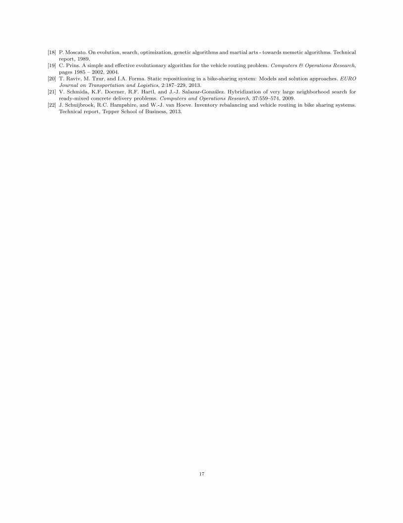
Figure 4. With Q := 2, M := +∞, T := 5, an example of instance for which the optimal

values of the relaxations (RP)=

and (RP)≥

differ

Appendix

This appendix deals with the impact of relaxing the equality to inequality constraints in the relaxation

proposed in Section 3. We denote as (RP)=

and (RP)≥

the two linear programs. While in traditional VehicleRouting Problems, this change has no impact on the optimal value of the relaxation, in our MVBP it could.

In fact, consider a network as that of Figure 4. The number near each vertex i corresponds to di. Thenumber near each edge, instead, represents the shortest-path distance between the two endpoints, that is1 for the edges incident to the depot, and δ � 1 for the others. The other parameters are set as follows:Q := 2, M := +∞, T := 5.

It is easy to check that no schedules except the following may be selected in an optimal solution of either

(RP)=

or (RP)≥

.rs ls cs

s1 (v1, v2, v3, v4) (2, 2, 1, 1) 2 + 4δs2 (v1, v4, v3, v2) (1, 1, 2, 2) 2 + 4δs3 (v5, v6, v7, v8) (1, 1, 2, 2) 2 + 4δs4 (v5, v8, v7, v6) (1, 1, 2, 2) 2 + 4δs5 (v1, v2, v3, v6) (2, 2, 2, 2) 4 + 6δs6 (v1, v4, v3, v6) (2, 1, 1, 2) 4 + 6δ

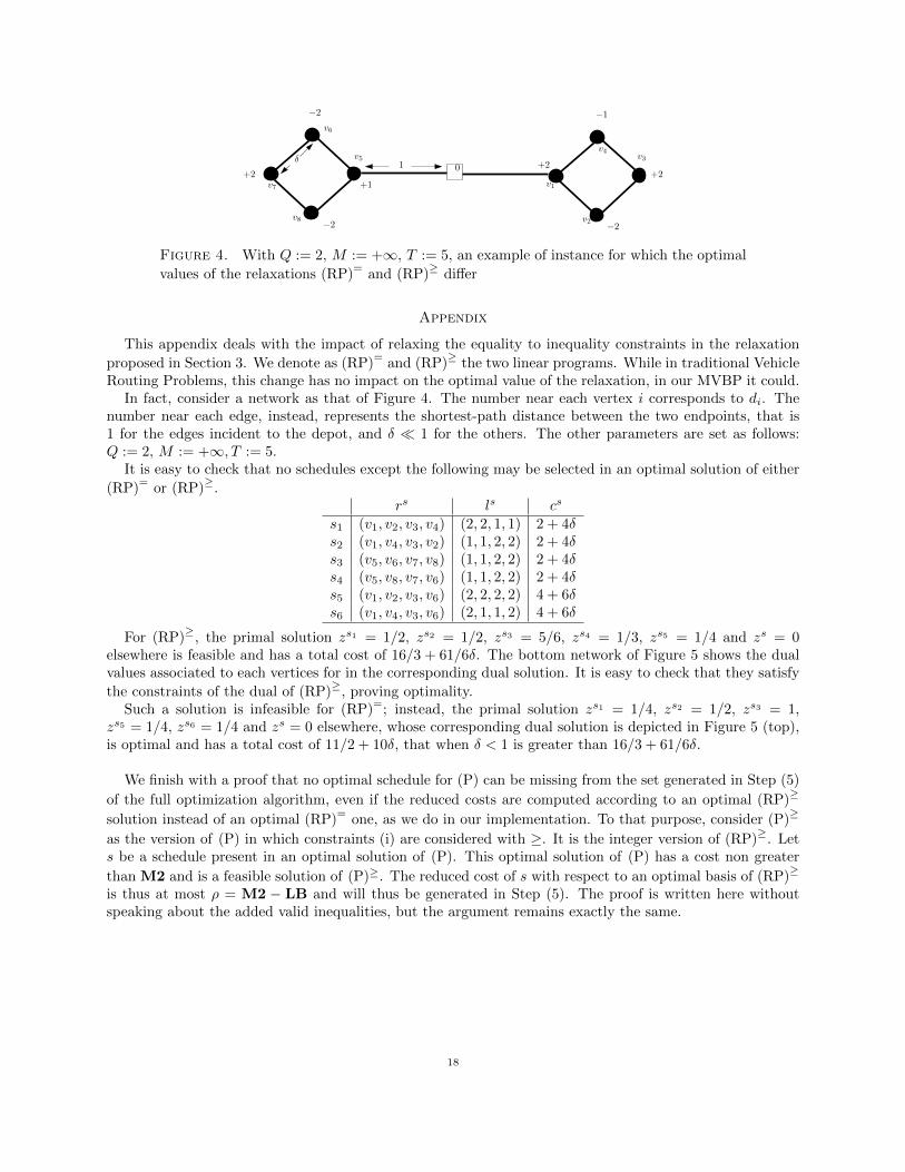
For (RP)≥

, the primal solution zs1 = 1/2, zs2 = 1/2, zs3 = 5/6, zs4 = 1/3, zs5 = 1/4 and zs = 0elsewhere is feasible and has a total cost of 16/3 + 61/6δ. The bottom network of Figure 5 shows the dualvalues associated to each vertices for in the corresponding dual solution. It is easy to check that they satisfy

the constraints of the dual of (RP)≥

, proving optimality.Such a solution is infeasible for (RP)

=; instead, the primal solution zs1 = 1/4, zs2 = 1/2, zs3 = 1,

zs5 = 1/4, zs6 = 1/4 and zs = 0 elsewhere, whose corresponding dual solution is depicted in Figure 5 (top),is optimal and has a total cost of 11/2 + 10δ, that when δ < 1 is greater than 16/3 + 61/6δ.

We finish with a proof that no optimal schedule for (P) can be missing from the set generated in Step (5)

of the full optimization algorithm, even if the reduced costs are computed according to an optimal (RP)≥

solution instead of an optimal (RP)=

one, as we do in our implementation. To that purpose, consider (P)≥

as the version of (P) in which constraints (i) are considered with ≥. It is the integer version of (RP)≥

. Lets be a schedule present in an optimal solution of (P). This optimal solution of (P) has a cost non greater

than M2 and is a feasible solution of (P)≥. The reduced cost of s with respect to an optimal basis of (RP)≥

is thus at most ρ = M2 − LB and will thus be generated in Step (5). The proof is written here withoutspeaking about the added valid inequalities, but the argument remains exactly the same.

18

0(RP)≥

(RP)= 0

− 12

23 (1 + 2δ)

0

32δ

0

0

32 + 2δ

−1− δ

32 + 2δ

1 + 2δ

0

0

0

23 (1 + 2δ)

13 (2 +

52δ)

13 (2 +

52δ)

Figure 5. Feasible dual solutions of (RP)=

and (RP)≥

, which can be proved to be optimal

19