Type II robotic assembly line balancing problem: An evolution strategies algorithm for a multi-objective model

T

Ta

AD

a

ARRAA

KRMPM

1

1

cfro

itaius

iwcsB

w

0d

Journal of Manufacturing Systems 31 (2012) 139– 151

Contents lists available at SciVerse ScienceDirect

Journal of Manufacturing Systems

jo u r n al hom epa ge: www.elsev ier .com/ locate / jmansys

echnical paper

ype II robotic assembly line balancing problem: An evolution strategieslgorithm for a multi-objective model

. Yoosefelahi, M. Aminnayeri ∗, H. Mosadegh, H. Davari Ardakaniepartment of Industrial Engineering, Amirkabir University of Technology, 424 Hafez Ave., Tehran 15916-34311, Iran

r t i c l e i n f o

rticle history:eceived 8 February 2011eceived in revised form 3 July 2011ccepted 10 October 2011

a b s t r a c t

In this paper a different type II robotic assembly line balancing problem (RALB-II) is considered. One ofthe two main differences with the existing literature is objective function which is a multi-objective one.The aim is to minimize the cycle time, robot setup costs and robot costs. The second difference is on theprocedure proposed to solve the problem. In addition, a new mixed-integer linear programming model is

vailable online 28 October 2011

eywords:obotic assembly line balancingulti-objective evolution strategies

areto optimal

developed. Since the problem is NP-hard, three versions of multi-objective evolution strategies (MOES)are employed. Numerical results show that the proposed hybrid MOES is more efficient.

© 2011 The Society of Manufacturing Engineers. Published by Elsevier Ltd. All rights reserved.

ixed-integer linear programming

. Introduction

.1. RALB problem description

The growing need for flexible production which is caused byompetitive markets and customers demand for more variety, callsor flexible assembly systems in which, robots play an importantole. A main configuration of robots in flexible systems, is the usef robotic assembly lines [1].

Assembly lines are flow-oriented production systems in thendustrial production of high quantity, standardized commodi-ies and low volume production of customized products [2]. Anssembly robot can work with no weariness. The goals of robotmplementation include a high productivity, a good quality of prod-cts, the manufacturing flexibility, the safety and a less demand forkilled labour [3].

The simple assembly line balancing (SALB) problem is the build-ng block of this family of problems. SALB problems are those, in

hich, tasks are assigned to workstations such that precedenceonstraints between tasks or other constraints are met. Table 1hows different versions of SALB problems presented by Scholl andecker [2]. All the versions are NP-hard [4].

An assembly robot could be programmed to do different jobs,hile another assembly robot may do same jobs with different

∗ Corresponding author. Tel.: +98 21 66413034.E-mail address: [email protected] (M. Aminnayeri).

278-6125/$ – see front matter © 2011 The Society of Manufacturing Engineers. Publisheoi:10.1016/j.jmsy.2011.10.002

efficiencies. Therefore, a wise allocation of robots to workstationsis essential for a high performance of an assembly line.

A robotic assembly line balancing (RALB) problem is a problemof efficiently assigning tasks and allocating robots to workstations.There are two types of RALB problems, namely, type I and type II.

In type I robotic assembly line balancing (RALB-I) problems, witha given cycle time, the objective is to minimize the number of work-stations or the cost of the assembly line. A type II robotic assemblyline balancing (RALB-II) problem uses different robot types to per-form assembly tasks. Each robot type has different processing timedue to its capability and specialization.

This paper provides a new mixed-integer linear programming(MILP) model for an RALB-II problem. In the presented model, threeobjective functions, namely, the cycle time, the robot setup cost andthe robot cost, are considered to be minimized, simultaneously.Because of the NP-hardness, a meta-heuristic algorithm, evolu-tion strategies (ES), is utilized. For this purpose, three versions ofmulti-objective ES are employed for solving some test problemsobtained from the literature. Four well-known performance mea-sures are used to show that our proposed algorithm outperformsothers.

1.2. Literature review

The model of Graves and Lamar [5] is on selecting workstations
from a set of non-identical candidates and assigning tasks to theselected workstations, simultaneously. Their objective is to mini-mize the total cost of the system. Pinto et al. [6] work is about thedesign of an assembly line with identical and parallel machines.
d by Elsevier Ltd. All rights reserved.

dx.doi.org/10.1016/j.jmsy.2011.10.002

http://www.sciencedirect.com/science/journal/02786125

http://www.elsevier.com/locate/jmansys

mailto:[email protected]

dx.doi.org/10.1016/j.jmsy.2011.10.002

140 A. Yoosefelahi et al. / Journal of Manufact

Table 1Versions of SALB.

Versions of SALB Cycle time (ct) No. ofworkstations (K)

Objective

SALB-F Given Given To establishwhether or not afeasible linebalance exists for agiven combinationof K and ct

SALB-1 Given ? To minimize KSALB-2 ? Given To minimize ctSALB-E ? ? To minimize ct and

rii

bOEo

1

tdedtip

mfatvNv

2

a

TP

K simultaneouslyconsidering theirinterrelationship

Khouja et al. [7] propose a two-stage methodology to designobotic assembly cells. Other works on RALB area are summarizedn Table 2, which gives a brief and thorough view of previous stud-es.

Regarding evolution strategies, comprehensive studies haveeen done by Beyer and Schwefel [8], Bäck [9] and Costa andliveira [10]. Costa and Oliveira [11] provide an adaptive sharingS for multi-objective optimization. For more details about multi-bjective techniques, one can refer to [12,13,14].

.3. Gap analysis

In practice, a decision maker may consider more than one objec-ive, especially, in strategic plans such as robotic assembly lineesigns. Regardless of the robot cost, all previous studies consid-red only one objective. Considering the robot costs, this paperevelops a new mixed-integer linear programming model withhree well-known objective functions for the problem. In addition,t provides a new scheme of solution representation to deal with theroblem via three versions of multi-objective evolution strategies.

The rest of this paper is organized as follows. In Section 2 theulti-objective type II robotic assembly line balancing problem is

ormulated. Section 3 is devoted to evolution strategies, encodingnd decoding methods and the proposed search techniques. In Sec-ion 4, the problem is analyzed from the multi-objective point ofiew, and the procedure of dealing with that is discussed there.umerical results of solving some available test problems are pro-ided in Section 5. Finally, Section 6 concludes the paper.

. Multi-objective type II RALB problem formulation

To produce a given product, a certain number of indivisiblessembly tasks are needed, say J tasks. There are some precedence

able 2revious works on RALB.

Article Cycle time (ct) Model

Nicosia et al. [7] Given Assigning tasks tonon-identical workstationssubject to precedenceconstraints.

Rubinovitz andBukchin [8]

Given Formulate the RALB problem

Rubinovitz et al. [9] Given Formulate the RALB problem

Bukchin and Tzur[10]

Given Formulate the RALB problem

Levitin et al. [1] ? A type II RALB problem

Gao et al. [3] ? A type II RALB problem

uring Systems 31 (2012) 139– 151

constraints which determine the order in which tasks could be per-formed. The assembly line has K serial workstations with a robot ineach.

At first, this model aims to create an assembly line which doesnot exist. Let J assembly tasks and K workstations are given. Theaim is to determine types of robots that should be bought suchthat the total cost of robots is minimized. Achieving an optimaldecision needs three questions to be answered. How to assign tasksto workstations?, which type of robot has to be bought?, and how toallocate robots to workstations? Three objectives to be minimizedare: cycle time, robot setup cost and robot cost.

The following assumptions considered in the model formulationare of those mentioned by Levitin et al. [1] and Gao et al. [3].

(1) The precedence relations among assembly tasks are knownand invariable. This precedence is represented by a prece-dence graph.

(2) There are only r types of robot available (r ≥ 1), but within eachtype, there is no limitation on the number of robots available,i.e., there are at least K robots of each type.

(3) The processing time of an assembly task depends on the allo-cated robot type.

(4) There is no limitation on assignment of an assembly task toany workstation other than precedence constraints.

(5) A single robot is allocated to each workstation.(6) Each robot type necessarily does not have the ability to per-

form any assembly task. In a case that processing of anassembly task on a specified robot is not desired, the setupcost of the robot for that task is set infinity.

(7) Material handling, loading and unloading times are negligible,or are included in processing times.

(8) Due to time consuming nature of setups, robot setup times areconsidered.

(9) It is assumed that purchasing more than one robot of any typewill have a discount, with a fixed and known rate related tothat robot type.

(10) The purchase cost of robots is considered.(11) The line is balanced for a single product.

Assumptions (2), (6), (8), (9), and (10) are of our own.The following notations will be used.Set of parameters:

J: number of assembly tasks with j = 1, 2, . . ., J
K: number of workstations with k = 1, 2, . . ., KR: number of robot types with r = 1, 2, . . ., Rprc(j): set of immediate predecessors of task j with h ∈ prc(j)tjr: processing time of task j by robot type r
Objective Solution procedure

To minimize the cost of theworkstations

A dynamic programmingalgorithm

To minimize the number ofworkstations

–

To minimize the number ofworkstations

A branch & bound algorithm

To minimize the totalequipment cost

An exact and heuristic branch& bound

To assign tasks to workstationsand to select the best fit robottype for each workstation suchthat cycle time is minimized

Two GA versions

To minimize cycle time A hybrid genetic algorithm

nufact

X

Y

m

m

m

∑

∑

∑

∑

∑∑

X

Y

mtchsdocrt

A. Yoosefelahi et al. / Journal of Ma

� r: discount rate of robot type r, 0 ≤ � r < 1Cr: cost of a robot of type r, to be purchasedSCrj: setup cost of a robot of type r, for processing task j : a very large positive number

Set of decision variables:

jkr ={

1 if the task j is assigned to the workstation kand the robot type r is allocated to the workstation k,

0 otherwise.

kr ={

1 if the robot type r is allocated to the workstation k,0 otherwise.

ct: cycle timeNow, the multi-objective RALB-II is formulated as follows:

in Z1 = ct (1)

in Z2 =R∑r=1

K∑k=1

J∑j=1

SCrjXjkr (2)

in Z3 =R∑r=1

Cr

(1 + �r(

K∑k=1

Ykr − 1)

)(3)

Subject to:

J

j=1

R∑r=1

tjrXjkr ≤ ct k = 1, 2, . . . , K (4)

K

k=1

R∑r=1

k.Xhkr −K∑k=1

R∑r=1

k.Xjkr ≤ 0 ∀ h ∈ prc(j) (5)

K

k=1

R∑r=1

Xjkr = 1 j = 1, 2, . . . , J (6)

J

j=1

Xjkr ≤ .Ykr k = 1, 2, . . . , K; r = 1, 2, . . . , R (7)

R

r=1

Ykr ≤ 1 k = 1, 2, . . . , K (8)

K

k=1

R∑r=1

Ykr ≤ K (9)

jkr ∈ {0, 1} j = 1, 2, . . . , J ; k = 1, 2, . . . , K ; r = 1, 2, . . . , R

(10)

kr ∈ {0, 1} k = 1, 2, . . . , K ; r = 1, 2, . . . , R (11)

Objective (1) is to minimize the cycle time. Objective (2) is toinimize the total robot setup cost and objective (3) is to minimize

he total robot cost (purchasing cost). Constraint (4) computes theycle time. Inequality (5) ensures that precedence constraints areeld, i.e., considering a pair of jobs with precedence relations, theuccessor could not be assigned to a workstation before the prece-ent job. Eq. (6) ensures that each assembly task is assigned only to
ne workstation. Inequality (7) indicates the type of robot to be allo-ated to a given workstation. Constraint (8) enforces that only oneobot can be assigned to a workstation. Inequality (9) shows thathe total number of robots used, regardless of their types, should
uring Systems 31 (2012) 139– 151 141

be at most equal to the number of workstations. Constraints (10)and (11) show binary variables.

3. Evolution strategies

Since all versions of SALB problems are NP-hard [4], our prob-lem is also NP-hard. Therefore, it is necessary to use meta-heuristicalgorithms for large-scale problems. We chose to apply evolutionstrategies for solving this problem. A vector of real-valued enti-ties is considered as the proposed chromosome. ES is selected,since the proposed solution scheme is continuous and we arealso looking for a population-based algorithm. In fact, ES employsadvantages of both simulated annealing (mutation) and geneticalgorithm (recombination).

3.1. Well-known types of ES

ES usually needs a less population size than GA. There are dif-ferent variants of ES. Some of the most prominent and applicableones are:

(� + �) − ES: In this type all the � parents and � offsprings aresorted and the best first � individuals would be chosen to go to thenext generation.

(�, �) − ES: In this type only � offsprings are sorted and the bestfirst � individuals would be chosen to go to the next generation.

Other types of ES are like (� + 1) − ES or (1 + 1) − ES, which arespecial cases of (� + �) − ES.

3.2. Solution representation

In the presented ES, a chromosome is defined as a (1 × J) vector,say x, where J is the number of assembly tasks. Any element ofthe mentioned array, say xi is a random real-valued number withininterval (1, K + 1), where K is the number of workstations.

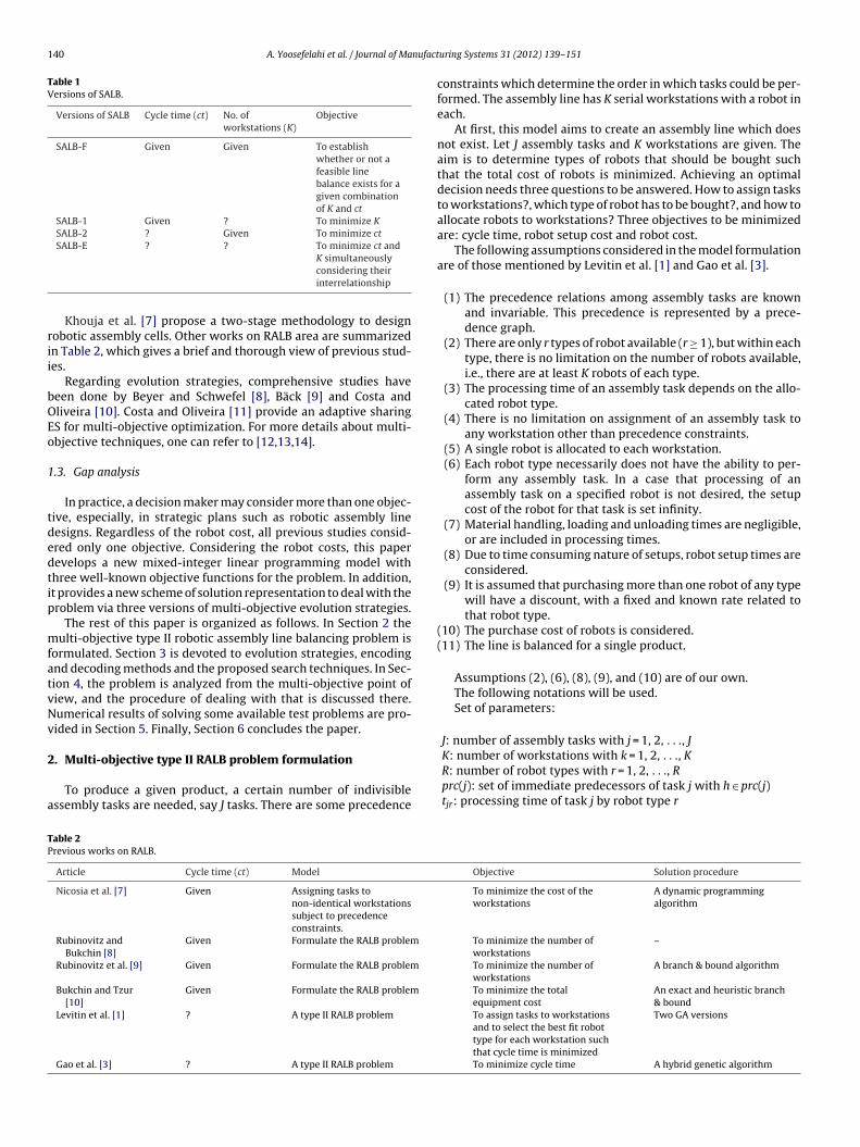
An example of the proposed individual is shown in Fig. 1.In this example there are 10 assembly tasks and 5 worksta-tions. The sample individual is a (1 × 10) vector with 10 randomreal-valued numbers within interval (1, 6) as its elements. Toexplore the search space we consider four decimal places for eachnumber.

3.3. Decoding procedure

The procedure is always started with a feasible solution.Because the random generated vector is sorted in ascendingorder and hence the precedence constraints are met. Basi-cally, any chromosome contains three main information of theproblem. They are tasks assignment, robot assignment androbot types. The aim of the proposed decoding procedure isto extract the three mentioned information from the chro-mosome. The procedure is represented in the following threesteps.

Step 1 (.). Assigning assembly tasks to workstations

Consider the primary generated individual, the (1 × J) vector.Each of the J assembly tasks, represented as a real-valued numberin a vector, is shown in Fig. 1 (the xi quantities). The workstation,which the assembly task should be assigned to, is the integer partof each xi in the individual vector. For example, the real-valuednumber for assembly task 1 shown in Fig. 1 is 1.2834 and its inte-ger part is 1. So, the assembly task 1 is assigned to the workstation
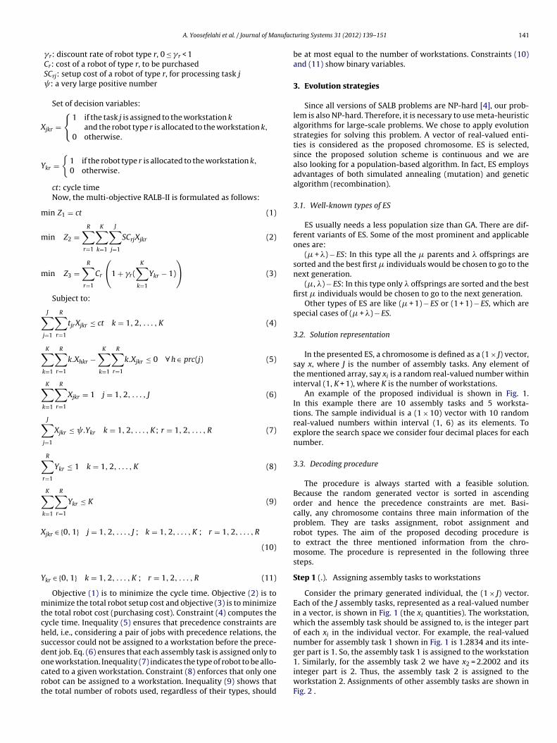
1. Similarly, for the assembly task 2 we have x2 = 2.2002 and itsinteger part is 2. Thus, the assembly task 2 is assigned to theworkstation 2. Assignments of other assembly tasks are shown inFig. 2 .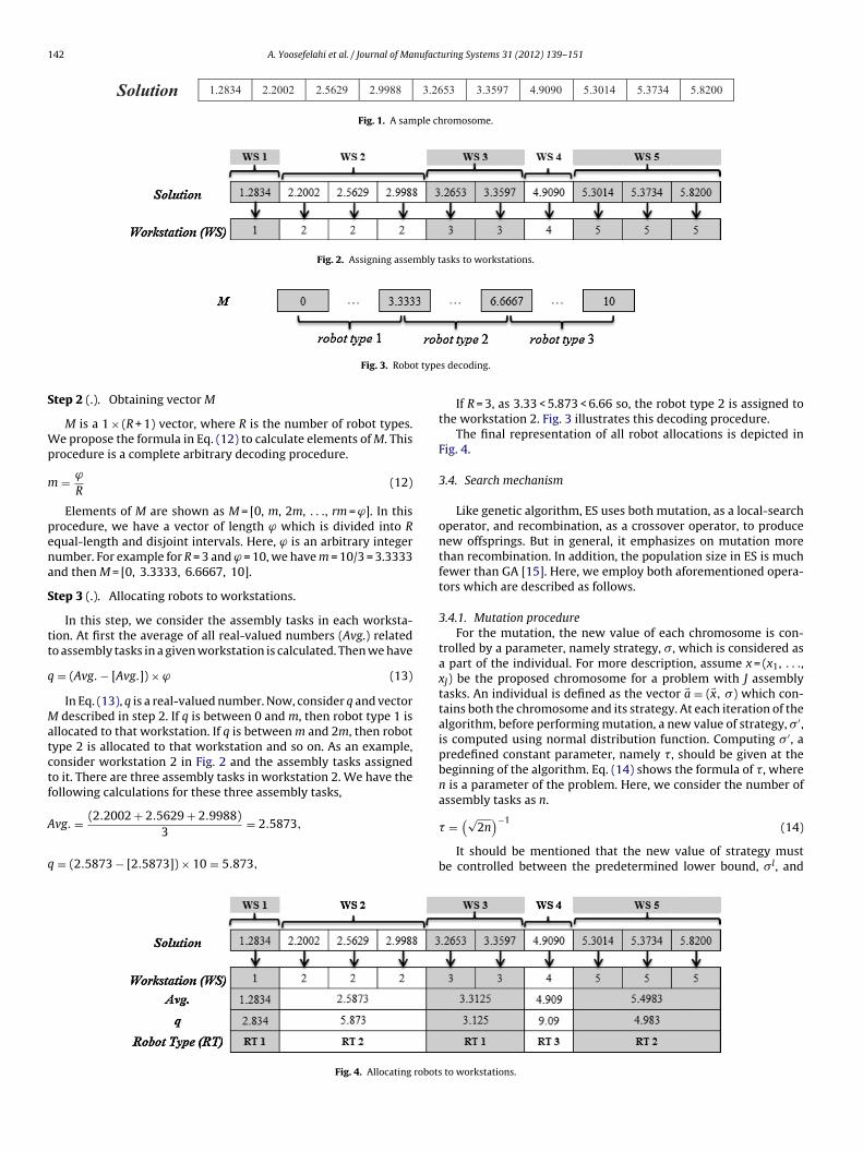

142 A. Yoosefelahi et al. / Journal of Manufacturing Systems 31 (2012) 139– 151

Solution 1.283 4 2.200 2 2.562 9 2.998 8 3.265 3 3.359 7 4.909 0 5.301 4 5.373 4 5.820 0

Fig. 1. A sample chromosome.

Fig. 2. Assigning assembly tasks to workstations.

t type

S

Wp

m

pena

S

tt

q

Matctf

A

q

Fig. 3. Robo

tep 2 (.). Obtaining vector M

M is a 1 × (R + 1) vector, where R is the number of robot types.e propose the formula in Eq. (12) to calculate elements of M. This

rocedure is a complete arbitrary decoding procedure.

= ϕ

R(12)

Elements of M are shown as M = [0, m, 2m, . . ., rm = ϕ]. In thisrocedure, we have a vector of length ϕ which is divided into Rqual-length and disjoint intervals. Here, ϕ is an arbitrary integerumber. For example for R = 3 and ϕ = 10, we have m = 10/3 = 3.3333nd then M = [0, 3.3333, 6.6667, 10].

tep 3 (.). Allocating robots to workstations.

In this step, we consider the assembly tasks in each worksta-ion. At first the average of all real-valued numbers (Avg.) relatedo assembly tasks in a given workstation is calculated. Then we have

= (Avg. − [Avg.]) × ϕ (13)

In Eq. (13), q is a real-valued number. Now, consider q and vector described in step 2. If q is between 0 and m, then robot type 1 is

llocated to that workstation. If q is between m and 2m, then robotype 2 is allocated to that workstation and so on. As an example,onsider workstation 2 in Fig. 2 and the assembly tasks assignedo it. There are three assembly tasks in workstation 2. We have theollowing calculations for these three assembly tasks,

vg. = (2.2002 + 2.5629 + 2.9988)3

= 2.5873,

= (2.5873 − [2.5873]) × 10 = 5.873,

Fig. 4. Allocating robots

s decoding.

If R = 3, as 3.33 < 5.873 < 6.66 so, the robot type 2 is assigned tothe workstation 2. Fig. 3 illustrates this decoding procedure.

The final representation of all robot allocations is depicted inFig. 4.

3.4. Search mechanism

Like genetic algorithm, ES uses both mutation, as a local-searchoperator, and recombination, as a crossover operator, to producenew offsprings. But in general, it emphasizes on mutation morethan recombination. In addition, the population size in ES is muchfewer than GA [15]. Here, we employ both aforementioned opera-tors which are described as follows.

3.4.1. Mutation procedureFor the mutation, the new value of each chromosome is con-

trolled by a parameter, namely strategy, �, which is considered asa part of the individual. For more description, assume x = (x1, . . .,xJ) be the proposed chromosome for a problem with J assemblytasks. An individual is defined as the vector �a = (�x, �) which con-tains both the chromosome and its strategy. At each iteration of thealgorithm, before performing mutation, a new value of strategy, � ′,is computed using normal distribution function. Computing � ′, apredefined constant parameter, namely �, should be given at thebeginning of the algorithm. Eq. (14) shows the formula of �, wheren is a parameter of the problem. Here, we consider the number ofassembly tasks as n.

� =(√

2n)−1

(14)

It should be mentioned that the new value of strategy mustbe controlled between the predetermined lower bound, � l, and

to workstations.

A. Yoosefelahi et al. / Journal of Manufact

ultm

cidsp

S

S

wtbactp

A1

w

t

3

irirn

Fig. 5. Feasible assembly task balancing.

pper bound, �u. In the case of violating the interval, the relativeower bound or upper bound will be used instead. Finally, based onhe new strategy, the new individual, �a′ = (�x′, � ′), is calculated by

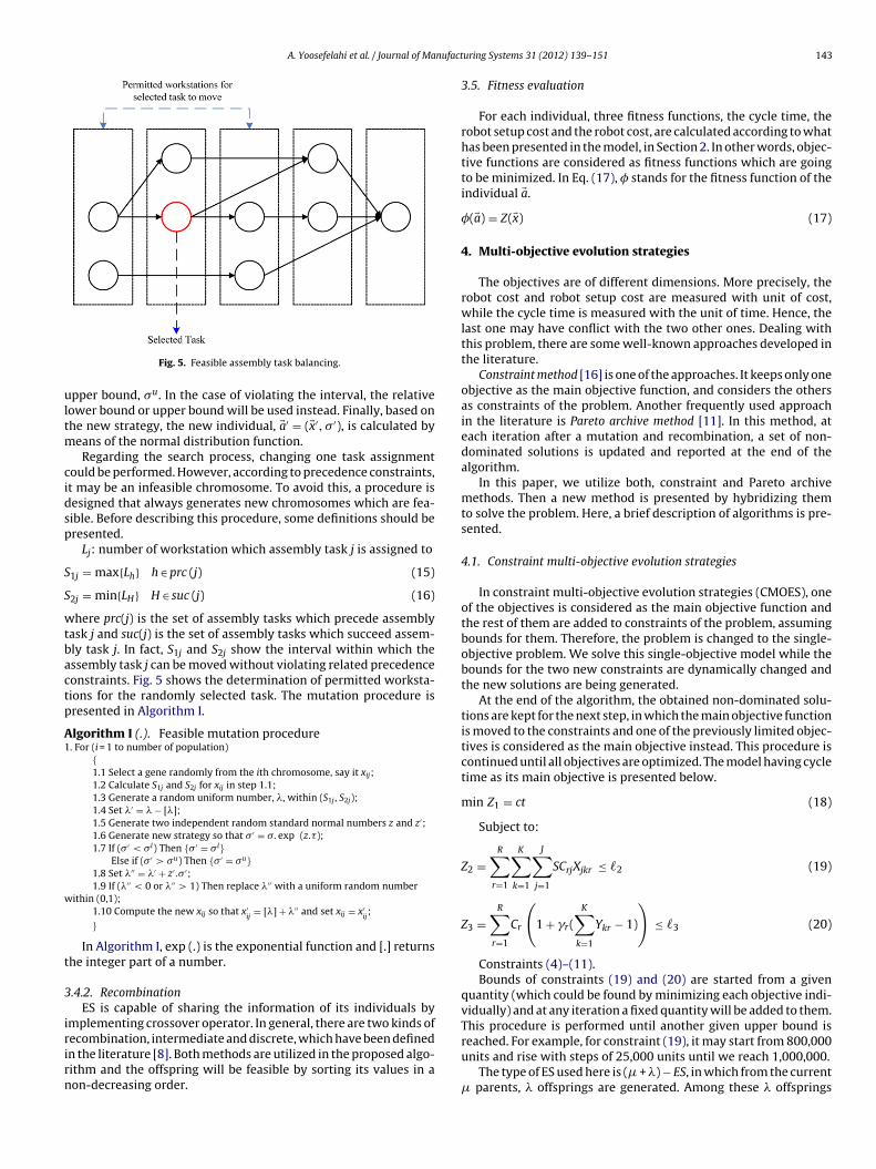
eans of the normal distribution function.Regarding the search process, changing one task assignment

ould be performed. However, according to precedence constraints,t may be an infeasible chromosome. To avoid this, a procedure isesigned that always generates new chromosomes which are fea-ible. Before describing this procedure, some definitions should beresented.

Lj: number of workstation which assembly task j is assigned to

1j = max{Lh} h ∈ prc (j) (15)

2j = min{LH} H ∈ suc (j) (16)

here prc(j) is the set of assembly tasks which precede assemblyask j and suc(j) is the set of assembly tasks which succeed assem-ly task j. In fact, S1j and S2j show the interval within which thessembly task j can be moved without violating related precedenceonstraints. Fig. 5 shows the determination of permitted worksta-ions for the randomly selected task. The mutation procedure isresented in Algorithm I.

lgorithm I (.). Feasible mutation procedure. For (i = 1 to number of population)

{1.1 Select a gene randomly from the ith chromosome, say it xij;1.2 Calculate S1j and S2j for xij in step 1.1;1.3 Generate a random uniform number, �, within (S1j , S2j);1.4 Set �′ = � − [�];1.5 Generate two independent random standard normal numbers z and z′;1.6 Generate new strategy so that � ′ = �. exp (z.�);1.7 If (� ′ < �l) Then {� ′ = �l}

Else if (� ′ > �u) Then {� ′ = �u}1.8 Set �′′ = �′ + z′.� ′;1.9 If (�′′ < 0 or �′′ > 1) Then replace �′′ with a uniform random number

ithin (0,1);1.10 Compute the new xij so that x′

ij= [�] + �′′ and set xij = x′

ij;

}

In Algorithm I, exp (.) is the exponential function and [.] returnshe integer part of a number.

.4.2. RecombinationES is capable of sharing the information of its individuals by

mplementing crossover operator. In general, there are two kinds of
ecombination, intermediate and discrete, which have been definedn the literature [8]. Both methods are utilized in the proposed algo-ithm and the offspring will be feasible by sorting its values in aon-decreasing order.
uring Systems 31 (2012) 139– 151 143

3.5. Fitness evaluation

For each individual, three fitness functions, the cycle time, therobot setup cost and the robot cost, are calculated according to whathas been presented in the model, in Section 2. In other words, objec-tive functions are considered as fitness functions which are goingto be minimized. In Eq. (17), � stands for the fitness function of theindividual �a.�(�a) = Z(�x) (17)

4. Multi-objective evolution strategies

The objectives are of different dimensions. More precisely, therobot cost and robot setup cost are measured with unit of cost,while the cycle time is measured with the unit of time. Hence, thelast one may have conflict with the two other ones. Dealing withthis problem, there are some well-known approaches developed inthe literature.

Constraint method [16] is one of the approaches. It keeps only oneobjective as the main objective function, and considers the othersas constraints of the problem. Another frequently used approachin the literature is Pareto archive method [11]. In this method, ateach iteration after a mutation and recombination, a set of non-dominated solutions is updated and reported at the end of thealgorithm.

In this paper, we utilize both, constraint and Pareto archivemethods. Then a new method is presented by hybridizing themto solve the problem. Here, a brief description of algorithms is pre-sented.

4.1. Constraint multi-objective evolution strategies

In constraint multi-objective evolution strategies (CMOES), oneof the objectives is considered as the main objective function andthe rest of them are added to constraints of the problem, assumingbounds for them. Therefore, the problem is changed to the single-objective problem. We solve this single-objective model while thebounds for the two new constraints are dynamically changed andthe new solutions are being generated.

At the end of the algorithm, the obtained non-dominated solu-tions are kept for the next step, in which the main objective functionis moved to the constraints and one of the previously limited objec-tives is considered as the main objective instead. This procedure iscontinued until all objectives are optimized. The model having cycletime as its main objective is presented below.

min Z1 = ct (18)

Subject to:

Z2 =R∑r=1

K∑k=1

J∑j=1

SCrjXjkr ≤ 2 (19)

Z3 =R∑r=1

Cr

(1 + �r(

K∑k=1

Ykr − 1)

)≤ 3 (20)

Constraints (4)–(11).Bounds of constraints (19) and (20) are started from a given

quantity (which could be found by minimizing each objective indi-vidually) and at any iteration a fixed quantity will be added to them.This procedure is performed until another given upper bound is
reached. For example, for constraint (19), it may start from 800,000units and rise with steps of 25,000 units until we reach 1,000,000.
The type of ES used here is (� + �) − ES, in which from the current� parents, � offsprings are generated. Among these � offsprings


const

tteotsg

tcdt

4

sPgoa[fieg

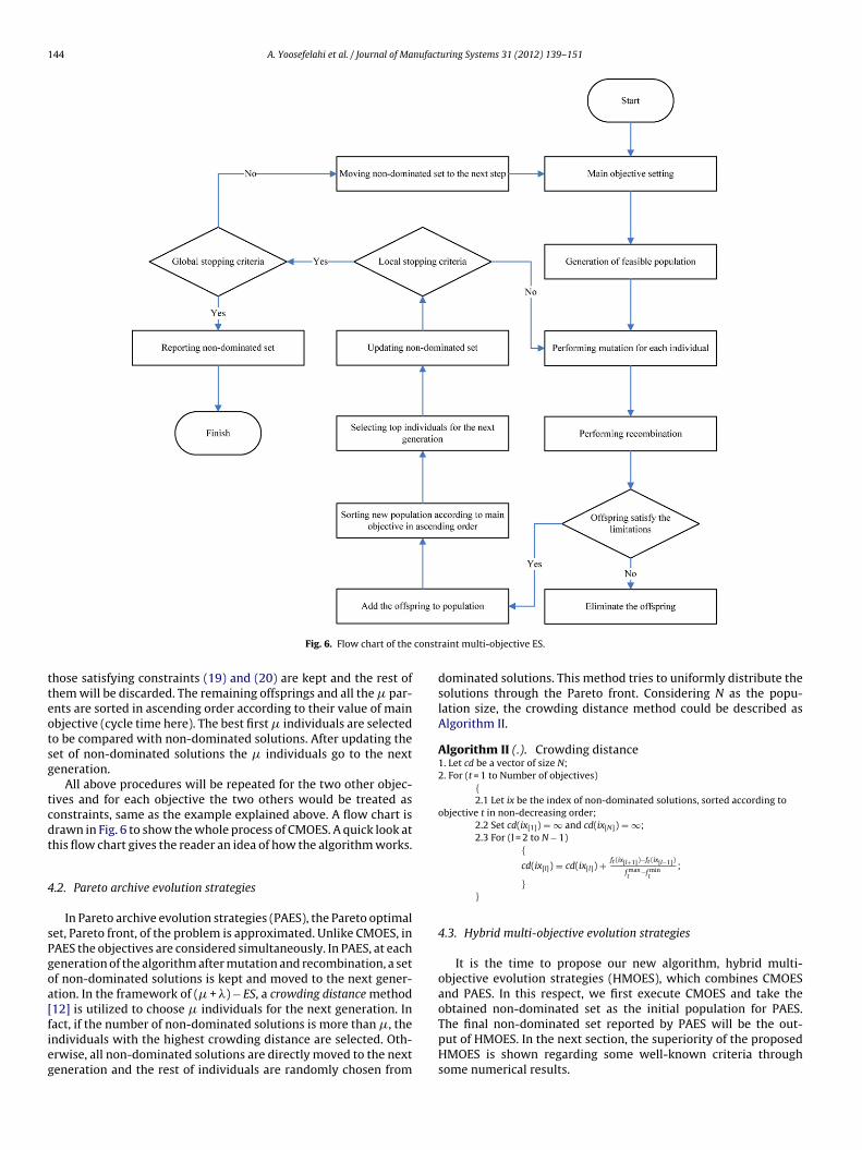
Fig. 6. Flow chart of the

hose satisfying constraints (19) and (20) are kept and the rest ofhem will be discarded. The remaining offsprings and all the � par-nts are sorted in ascending order according to their value of mainbjective (cycle time here). The best first � individuals are selectedo be compared with non-dominated solutions. After updating theet of non-dominated solutions the � individuals go to the nexteneration.

All above procedures will be repeated for the two other objec-ives and for each objective the two others would be treated asonstraints, same as the example explained above. A flow chart israwn in Fig. 6 to show the whole process of CMOES. A quick look athis flow chart gives the reader an idea of how the algorithm works.

.2. Pareto archive evolution strategies

In Pareto archive evolution strategies (PAES), the Pareto optimalet, Pareto front, of the problem is approximated. Unlike CMOES, inAES the objectives are considered simultaneously. In PAES, at eacheneration of the algorithm after mutation and recombination, a setf non-dominated solutions is kept and moved to the next gener-tion. In the framework of (� + �) − ES, a crowding distance method12] is utilized to choose � individuals for the next generation. In
act, if the number of non-dominated solutions is more than �, thendividuals with the highest crowding distance are selected. Oth-rwise, all non-dominated solutions are directly moved to the nexteneration and the rest of individuals are randomly chosen from
raint multi-objective ES.

dominated solutions. This method tries to uniformly distribute thesolutions through the Pareto front. Considering N as the popu-lation size, the crowding distance method could be described asAlgorithm II.

Algorithm II (.). Crowding distance1. Let cd be a vector of size N;2. For (t = 1 to Number of objectives)

{2.1 Let ix be the index of non-dominated solutions, sorted according to

objective t in non-decreasing order;2.2 Set cd(ix[1]) = ∞ and cd(ix[N]) = ∞;2.3 For (l = 2 to N − 1)

{cd(ix[l]) = cd(ix[l]) + ft (ix[l+1])−ft (ix[l−1])

fmaxt

−fmint

;

}}

4.3. Hybrid multi-objective evolution strategies

It is the time to propose our new algorithm, hybrid multi-objective evolution strategies (HMOES), which combines CMOESand PAES. In this respect, we first execute CMOES and take theobtained non-dominated set as the initial population for PAES.
The final non-dominated set reported by PAES will be the out-put of HMOES. In the next section, the superiority of the proposedHMOES is shown regarding some well-known criteria throughsome numerical results.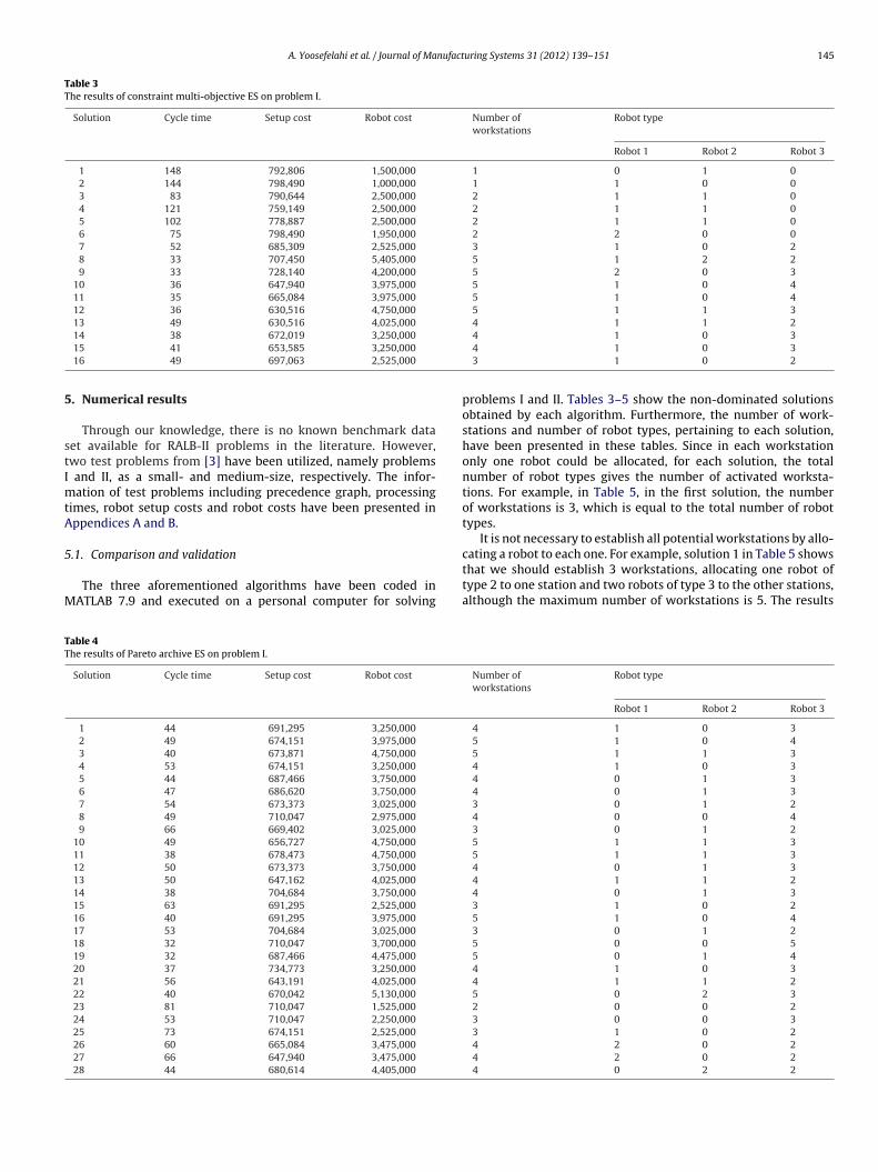

A. Yoosefelahi et al. / Journal of Manufacturing Systems 31 (2012) 139– 151 145

Table 3The results of constraint multi-objective ES on problem I.

Solution Cycle time Setup cost Robot cost Number ofworkstations

Robot type

Robot 1 Robot 2 Robot 3

1 148 792,806 1,500,000 1 0 1 02 144 798,490 1,000,000 1 1 0 03 83 790,644 2,500,000 2 1 1 04 121 759,149 2,500,000 2 1 1 05 102 778,887 2,500,000 2 1 1 06 75 798,490 1,950,000 2 2 0 07 52 685,309 2,525,000 3 1 0 28 33 707,450 5,405,000 5 1 2 29 33 728,140 4,200,000 5 2 0 3

10 36 647,940 3,975,000 5 1 0 411 35 665,084 3,975,000 5 1 0 412 36 630,516 4,750,000 5 1 1 313 49 630,516 4,025,000 4 1 1 2

5

stImtA

5

M

TT

14 38 672,019 3,250,000

15 41 653,585 3,250,000

16 49 697,063 2,525,000

. Numerical results

Through our knowledge, there is no known benchmark dataet available for RALB-II problems in the literature. However,wo test problems from [3] have been utilized, namely problems

and II, as a small- and medium-size, respectively. The infor-ation of test problems including precedence graph, processing

imes, robot setup costs and robot costs have been presented inppendices A and B.

.1. Comparison and validation

The three aforementioned algorithms have been coded inATLAB 7.9 and executed on a personal computer for solving

able 4he results of Pareto archive ES on problem I.

Solution Cycle time Setup cost Robot cost

1 44 691,295 3,250,000

2 49 674,151 3,975,000

3 40 673,871 4,750,000

4 53 674,151 3,250,000

5 44 687,466 3,750,000

6 47 686,620 3,750,000

7 54 673,373 3,025,000

8 49 710,047 2,975,000

9 66 669,402 3,025,000

10 49 656,727 4,750,000

11 38 678,473 4,750,000

12 50 673,373 3,750,000

13 50 647,162 4,025,000

14 38 704,684 3,750,000

15 63 691,295 2,525,000

16 40 691,295 3,975,000

17 53 704,684 3,025,000

18 32 710,047 3,700,000

19 32 687,466 4,475,000

20 37 734,773 3,250,000

21 56 643,191 4,025,000

22 40 670,042 5,130,000

23 81 710,047 1,525,000

24 53 710,047 2,250,000

25 73 674,151 2,525,000

26 60 665,084 3,475,000

27 66 647,940 3,475,000

28 44 680,614 4,405,000

4 1 0 34 1 0 33 1 0 2

problems I and II. Tables 3–5 show the non-dominated solutionsobtained by each algorithm. Furthermore, the number of work-stations and number of robot types, pertaining to each solution,have been presented in these tables. Since in each workstationonly one robot could be allocated, for each solution, the totalnumber of robot types gives the number of activated worksta-tions. For example, in Table 5, in the first solution, the numberof workstations is 3, which is equal to the total number of robottypes.

It is not necessary to establish all potential workstations by allo-
cating a robot to each one. For example, solution 1 in Table 5 showsthat we should establish 3 workstations, allocating one robot oftype 2 to one station and two robots of type 3 to the other stations,although the maximum number of workstations is 5. The results
Number ofworkstations

Robot type


4 1 0 35 1 0 45 1 1 34 1 0 34 0 1 34 0 1 33 0 1 24 0 0 43 0 1 25 1 1 35 1 1 34 0 1 34 1 1 24 0 1 33 1 0 25 1 0 43 0 1 25 0 0 55 0 1 44 1 0 34 1 1 25 0 2 32 0 0 23 0 0 33 1 0 24 2 0 24 2 0 24 0 2 2


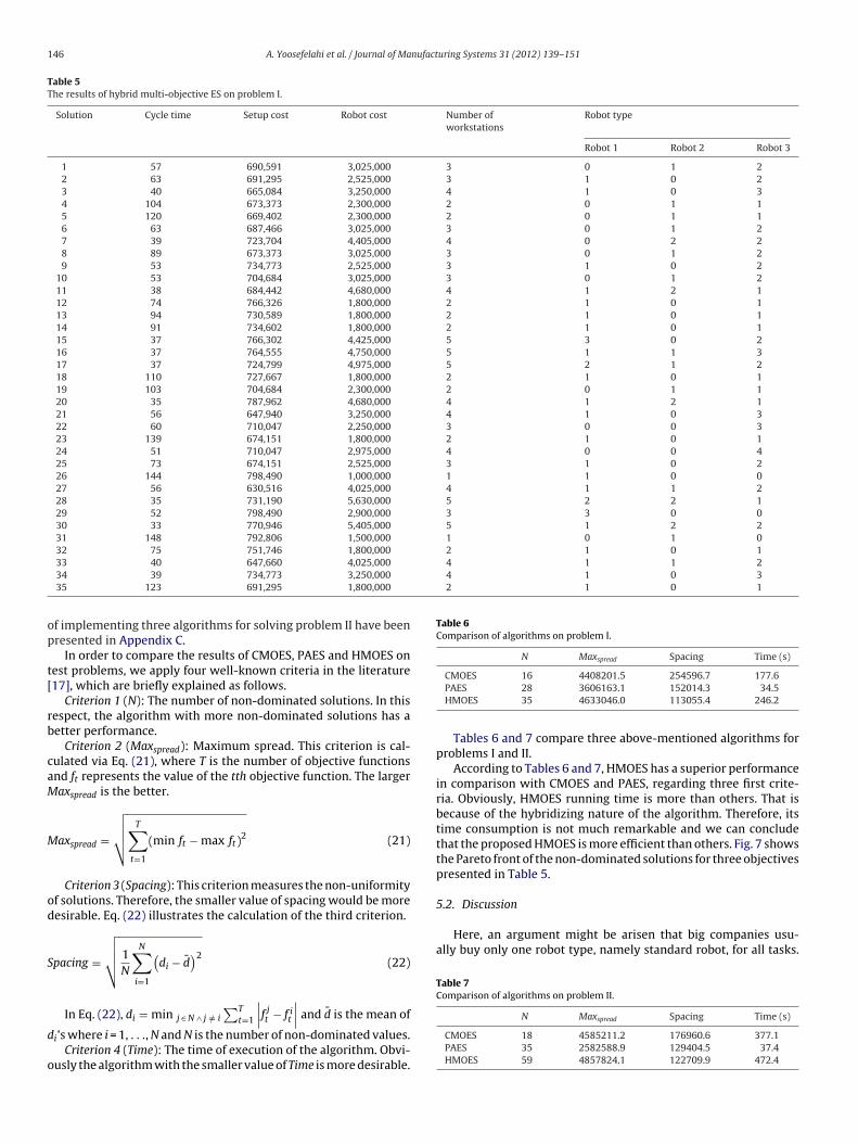
Table 5The results of hybrid multi-objective ES on problem I.


Robot type


1 57 690,591 3,025,000 3 0 1 22 63 691,295 2,525,000 3 1 0 23 40 665,084 3,250,000 4 1 0 34 104 673,373 2,300,000 2 0 1 15 120 669,402 2,300,000 2 0 1 16 63 687,466 3,025,000 3 0 1 27 39 723,704 4,405,000 4 0 2 28 89 673,373 3,025,000 3 0 1 29 53 734,773 2,525,000 3 1 0 2

10 53 704,684 3,025,000 3 0 1 211 38 684,442 4,680,000 4 1 2 112 74 766,326 1,800,000 2 1 0 113 94 730,589 1,800,000 2 1 0 114 91 734,602 1,800,000 2 1 0 115 37 766,302 4,425,000 5 3 0 216 37 764,555 4,750,000 5 1 1 317 37 724,799 4,975,000 5 2 1 218 110 727,667 1,800,000 2 1 0 119 103 704,684 2,300,000 2 0 1 120 35 787,962 4,680,000 4 1 2 121 56 647,940 3,250,000 4 1 0 322 60 710,047 2,250,000 3 0 0 323 139 674,151 1,800,000 2 1 0 124 51 710,047 2,975,000 4 0 0 425 73 674,151 2,525,000 3 1 0 226 144 798,490 1,000,000 1 1 0 027 56 630,516 4,025,000 4 1 1 228 35 731,190 5,630,000 5 2 2 129 52 798,490 2,900,000 3 3 0 030 33 770,946 5,405,000 5 1 2 231 148 792,806 1,500,000 1 0 1 032 75 751,746 1,800,000 2 1 0 1

4 1 1 24 1 0 32 1 0 1

op

t[

rb

caM

M

od

S

d

o

Table 6Comparison of algorithms on problem I.

N Maxspread Spacing Time (s)

5.2. Discussion

Here, an argument might be arisen that big companies usu-ally buy only one robot type, namely standard robot, for all tasks.

Table 7Comparison of algorithms on problem II.

33 40 647,660 4,025,000

34 39 734,773 3,250,000

35 123 691,295 1,800,000

f implementing three algorithms for solving problem II have beenresented in Appendix C.

In order to compare the results of CMOES, PAES and HMOES onest problems, we apply four well-known criteria in the literature17], which are briefly explained as follows.

Criterion 1 (N): The number of non-dominated solutions. In thisespect, the algorithm with more non-dominated solutions has aetter performance.

Criterion 2 (Maxspread): Maximum spread. This criterion is cal-ulated via Eq. (21), where T is the number of objective functionsnd ft represents the value of the tth objective function. The largeraxspread is the better.

axspread =

√√√√ T∑t=1

(min ft − max ft)2 (21)

Criterion 3 (Spacing): This criterion measures the non-uniformityf solutions. Therefore, the smaller value of spacing would be moreesirable. Eq. (22) illustrates the calculation of the third criterion.

pacing =

√√√√ 1N

N∑i=1

(di − d̄

)2(22)

∑T∣∣ j ∣∣

In Eq. (22), di = min j ∈ N ∧ j /= i t=1 ∣ft − f it ∣ and d̄ is the mean of

i’s where i = 1, . . ., N and N is the number of non-dominated values.Criterion 4 (Time): The time of execution of the algorithm. Obvi-

usly the algorithm with the smaller value of Time is more desirable.

CMOES 16 4408201.5 254596.7 177.6PAES 28 3606163.1 152014.3 34.5HMOES 35 4633046.0 113055.4 246.2

Tables 6 and 7 compare three above-mentioned algorithms forproblems I and II.

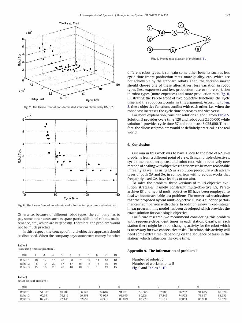
According to Tables 6 and 7, HMOES has a superior performancein comparison with CMOES and PAES, regarding three first crite-ria. Obviously, HMOES running time is more than others. That isbecause of the hybridizing nature of the algorithm. Therefore, itstime consumption is not much remarkable and we can concludethat the proposed HMOES is more efficient than others. Fig. 7 showsthe Pareto front of the non-dominated solutions for three objectivespresented in Table 5.

N Maxspread Spacing Time (s)

CMOES 18 4585211.2 176960.6 377.1PAES 35 2582588.9 129404.5 37.4HMOES 59 4857824.1 122709.9 472.4


Fig. 7. The Pareto front of non-dominated solutions obtained by HMOES.

F

Optn

b

TP

TS

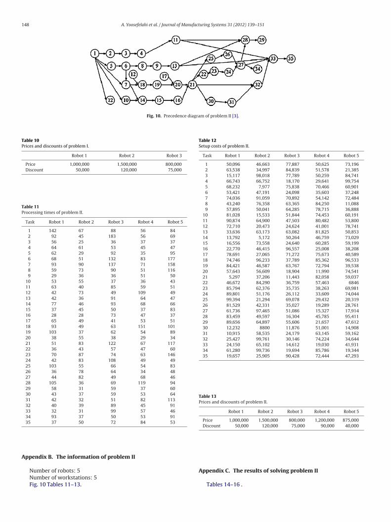
ig. 8. The Pareto front of non-dominated solution for cycle time and robot cost.

therwise, because of different robot types, the company has toay some other costs such as spare parts, additional robots, main-
enance, etc., which are very costly. Therefore, the problem wouldot be much practical.
In this respect, the concept of multi-objective approach shoulde discussed. When the company pays some extra money for other

able 8rocessing times of problem I.

Tasks 1 2 3 4 5 6 7 8 9 10

Robot 1 10 12 15 20 30 7 19 11 10 10Robot 2 8 10 20 17 17 16 15 16 19 10Robot 3 15 16 20 20 10 10 13 16 19 15

able 9etup costs of problem I.

Tasks 1 2 3 4 5

Robot 1 51,307 89,289 96,128 74,616 91,701Robot 2 60,651 76,116 69,868 73,955 99,695Robot 3 87,203 72,145 52,650 54,391 89,899

Fig. 9. Precedence diagram of problem I [3].

different robot types, it can gain some other benefits such as lesscycle time (more production rate), more quality, etc., which arenot achievable by the standard robots. Then, the decision makershould choose one of these alternatives: less variation in robottypes (less expenses) and less production rate or more variationin robot types (more expenses) and more production rate. Fig. 8,illustrating the Pareto front of two objective functions, the cycletime and the robot cost, confirms this argument. According to Fig.8, these objective functions conflict with each other, i.e., when therobot cost increases the cycle time decreases and vice versa.

For more explanation, consider solutions 1 and 5 from Table 5.Solution 5 provides cycle time 120 and robot cost 2,300,000 whilesolution 1 provides cycle time 57 and robot cost 3,025,000. There-fore, the discussed problem would be definitely practical in the realworld.

6. Conclusion

Our aim in this work was to have a look to the field of RALB-IIproblems from a different point of view. Using multiple objectives,cycle time, robot setup cost and robot cost, with a relatively newmethod of dealing with objectives that seems to be more reasonablein reality as well as using ES as a solution procedure with advan-tages of both GA and SA, in comparison with previous works thatfrequently used GA, have lead us to our aim.

To solve the problem, three versions of multi-objective evo-lution strategies, namely constraint multi-objective ES, Paretoarchive ES and hybrid multi-objective ES have been employed todeal with some available test problems. The numerical results showthat the proposed hybrid multi-objective ES has a superior perfor-mance in comparison with others. In addition, a new mixed-integerlinear programming model has been developed which provides theexact solution for each single objective.

For future research, we recommend considering this problemwith sequence-dependent times in each station. Clearly, in eachstation there might be a tool changing activity for the robot whichis necessary for two consecutive tasks. Therefore, this activity willneed some extra time (depending on the sequence of tasks in thestation) which influences the cycle time.

Appendix A. The information of problem I

Number of robots: 3Number of workstations: 5Fig. 9 and Tables 8–10

6 7 8 9 10

56,568 87,989 96,287 91,635 62,970 80,224 97,245 74,522 71,897 88,633 82,779 51,617 77,853 85,990 55,520


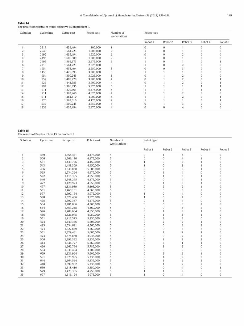
Fig. 10. Precedence diagram of problem II [3].

Table 10Prices and discounts of problem I.


Price 1,000,000 1,500,000 800,000Discount 50,000 120,000 75,000

Table 11Processing times of problem II.

Task Robot 1 Robot 2 Robot 3 Robot 4 Robot 5

1 142 67 88 56 842 92 45 183 56 693 56 25 36 37 374 64 61 53 45 475 62 29 92 35 956 68 51 132 83 1777 93 90 137 71 1588 59 73 90 51 1169 29 36 36 51 50

10 53 55 37 36 4311 63 40 85 59 5112 42 73 49 109 4913 42 36 91 64 4714 77 46 93 68 6615 37 45 50 37 8316 28 28 73 47 3717 65 49 41 53 5118 93 49 63 151 10119 103 37 62 54 8920 38 55 38 29 3421 51 83 122 67 11722 36 43 57 47 6023 70 87 74 63 14624 42 83 108 49 4925 103 55 66 54 8326 36 78 64 34 4827 44 82 49 68 4628 105 36 69 119 9429 58 31 59 37 6030 43 37 59 53 6431 42 32 51 82 11332 40 39 89 45 9133 32 31 99 57 4634 93 37 50 53 9135 37 50 72 84 53

A

Table 12Setup costs of problem II.

Task Robot 1 Robot 2 Robot 3 Robot 4 Robot 5

1 50,096 46,663 77,887 50,625 73,1962 63,538 34,997 84,839 51,578 21,3853 15,117 98,018 77,789 50,259 84,7414 66,743 66,752 18,170 29,641 99,7545 68,232 7,977 75,838 70,466 60,9016 53,421 47,191 24,098 35,603 37,2487 74,036 91,059 70,892 54,142 72,4848 43,240 76,358 63,365 84,250 11,0889 57,895 50,041 64,285 78,715 36,888

10 81,028 15,533 51,844 74,453 60,19111 90,874 64,900 47,503 80,482 53,80012 72,710 20,473 24,624 41,001 78,74113 33,636 63,173 63,082 81,825 50,85314 13,792 5,172 50,264 46,759 73,02915 16,556 73,558 24,640 60,285 59,19916 22,770 46,415 96,557 25,008 38,20817 78,691 27,065 71,272 75,673 40,58918 74,746 96,233 37,789 85,362 96,53319 84,421 46,587 63,767 72,794 39,53820 57,643 56,609 18,904 11,990 74,54121 5,297 37,206 11,443 82,058 59,03722 46,672 84,290 36,759 57,463 684623 85,794 62,376 35,735 38,263 69,98124 89,801 51,176 26,112 33,609 74,04425 99,394 21,294 69,078 29,432 20,31926 81,529 42,331 35,027 19,289 28,76127 61,736 97,465 51,086 15,327 17,91428 83,459 49,597 16,304 45,785 95,41129 89,656 64,897 55,606 21,657 47,61230 12,232 8800 11,876 51,001 14,90831 10,915 58,535 24,179 63,145 59,16232 25,427 99,761 30,146 74,224 34,64433 24,150 65,102 14,612 19,030 41,93134 61,280 99,736 19,694 85,786 19,34435 19,657 25,905 90,428 72,444 47,293

Table 13Prices and discounts of problem II.

Robot 1 Robot 2 Robot 3 Robot 4 Robot 5

Price 1,000,000 1,500,000 800,000 1,200,000 875,000Discount 50,000 120,000 75,000 90,000 40,000

ppendix B. The information of problem II

Number of robots: 5Number of workstations: 5Fig. 10 Tables 11–13.

Appendix C. The results of solving problem II

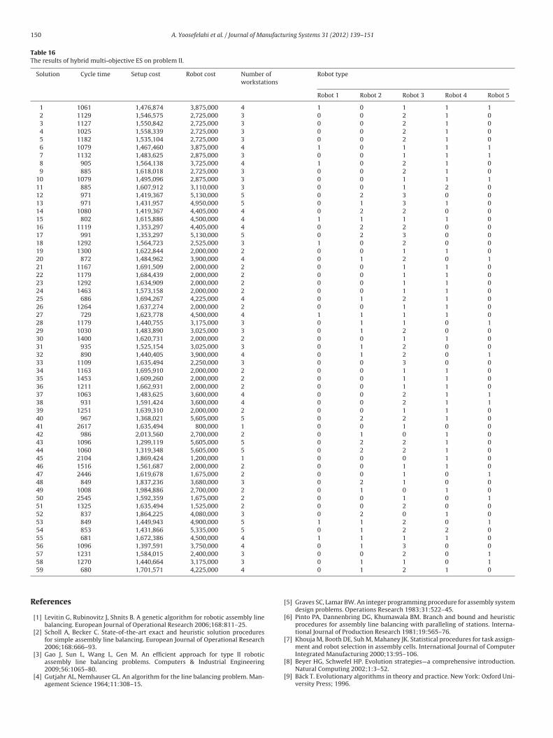
Tables 14–16 .


Table 14The results of constraint multi-objective ES on problem II.


Robot type


1 2617 1,635,494 800,000 1 0 0 1 0 02 2545 1,564,723 1,800,000 2 1 0 1 0 03 2495 1,635,494 1,525,000 2 0 0 2 0 04 2495 1,606,309 1,800,000 2 1 0 1 0 05 2495 1,564,373 2,675,000 3 1 0 1 0 16 2318 1,564,723 2,525,000 3 1 0 2 0 07 1954 1,635,494 2,250,000 3 0 0 3 0 08 1158 1,475,093 3,300,000 3 1 1 1 0 09 954 1,500,245 3,025,000 3 0 1 2 0 0

10 952 1,409,229 3,900,000 4 0 1 2 0 111 926 1,443,585 3,900,000 4 0 1 2 0 112 894 1,366,835 5,375,000 5 1 1 1 1 113 911 1,329,661 5,375,000 5 1 1 1 1 114 911 1,363,960 4,025,000 4 1 1 2 0 015 911 1,363,610 4,900,000 5 1 1 2 0 116 970 1,363,610 4,175,000 4 1 1 1 0 117 937 1,500,245 3,750,000 4 0 1 3 0 018 1259 1,635,494 2,975,000 4 0 0 4 0 0

Table 15The results of Pareto archive ES on problem I.


Robot type


1 489 1,554,431 4,475,000 5 0 1 4 0 02 506 1,569,180 4,175,000 5 0 0 4 1 03 581 1,439,736 4,450,000 5 1 0 3 1 04 543 1,488,309 4,450,000 5 1 0 3 1 05 466 1,346,858 5,605,000 5 0 2 2 1 06 525 1,534,264 4,475,000 5 0 1 4 0 07 522 1,418,395 4,950,000 5 0 1 3 1 08 546 1,548,295 4,175,000 5 0 0 4 1 09 477 1,420,923 4,950,000 5 0 1 3 1 0

10 477 1,331,989 5,605,000 5 0 2 2 1 011 531 1,460,181 4,560,000 5 0 0 3 2 012 577 1,597,164 3,975,000 5 1 0 4 0 013 580 1,528,466 3,975,000 5 1 0 4 0 014 478 1,597,387 4,475,000 5 0 1 4 0 015 504 1,481,066 4,560,000 5 0 0 3 2 016 534 1,451,238 4,560,000 5 0 0 3 2 017 576 1,408,604 4,950,000 5 0 1 3 1 018 456 1,526,045 4,950,000 5 0 1 3 1 019 551 1,417,575 5,130,000 5 0 2 3 0 020 424 1,349,386 5,605,000 5 0 2 2 1 021 485 1,534,621 4,560,000 5 0 0 3 2 022 474 1,627,839 4,560,000 5 0 0 3 2 023 551 1,329,461 5,605,000 5 0 2 2 1 024 473 1,578,850 4,945,000 5 0 0 2 3 025 506 1,393,392 5,335,000 5 0 1 2 2 026 413 1,544,777 6,260,000 5 0 3 1 1 027 420 1,662,794 5,785,000 5 0 3 2 0 028 584 1,635,494 3,700,000 5 0 0 5 0 029 659 1,321,964 5,605,000 5 0 2 2 1 030 591 1,375,995 5,335,000 5 0 1 2 2 031 644 1,364,524 5,335,000 5 0 1 2 2 032 448 1,599,902 5,335,000 5 0 1 2 2 033 650 1,618,410 3,850,000 5 0 0 4 0 134 529 1,478,385 4,750,000 5 1 1 3 0 035 697 1,516,124 3975,000 5 1 0 4 0 0


Table 16The results of hybrid multi-objective ES on problem II.


Robot type


1 1061 1,476,874 3,875,000 4 1 0 1 1 12 1129 1,546,575 2,725,000 3 0 0 2 1 03 1127 1,550,842 2,725,000 3 0 0 2 1 04 1025 1,558,339 2,725,000 3 0 0 2 1 05 1182 1,535,104 2,725,000 3 0 0 2 1 06 1079 1,467,460 3,875,000 4 1 0 1 1 17 1132 1,483,625 2,875,000 3 0 0 1 1 18 905 1,564,138 3,725,000 4 1 0 2 1 09 885 1,618,018 2,725,000 3 0 0 2 1 0

10 1079 1,495,096 2,875,000 3 0 0 1 1 111 885 1,607,912 3,110,000 3 0 0 1 2 012 971 1,419,367 5,130,000 5 0 2 3 0 013 971 1,431,957 4,950,000 5 0 1 3 1 014 1080 1,419,367 4,405,000 4 0 2 2 0 015 802 1,615,886 4,500,000 4 1 1 1 1 016 1119 1,353,297 4,405,000 4 0 2 2 0 017 991 1,353,297 5,130,000 5 0 2 3 0 018 1292 1,564,723 2,525,000 3 1 0 2 0 019 1300 1,622,844 2,000,000 2 0 0 1 1 020 872 1,484,962 3,900,000 4 0 1 2 0 121 1167 1,691,509 2,000,000 2 0 0 1 1 022 1179 1,684,439 2,000,000 2 0 0 1 1 023 1292 1,634,909 2,000,000 2 0 0 1 1 024 1463 1,573,158 2,000,000 2 0 0 1 1 025 686 1,694,267 4,225,000 4 0 1 2 1 026 1264 1,637,274 2,000,000 2 0 0 1 1 027 729 1,623,778 4,500,000 4 1 1 1 1 028 1179 1,440,755 3,175,000 3 0 1 1 0 129 1030 1,483,890 3,025,000 3 0 1 2 0 030 1400 1,620,731 2,000,000 2 0 0 1 1 031 935 1,525,154 3,025,000 3 0 1 2 0 032 890 1,440,405 3,900,000 4 0 1 2 0 133 1109 1,635,494 2,250,000 3 0 0 3 0 034 1163 1,695,910 2,000,000 2 0 0 1 1 035 1453 1,609,260 2,000,000 2 0 0 1 1 036 1211 1,662,931 2,000,000 2 0 0 1 1 037 1063 1,483,625 3,600,000 4 0 0 2 1 138 931 1,591,424 3,600,000 4 0 0 2 1 139 1251 1,639,310 2,000,000 2 0 0 1 1 040 967 1,368,021 5,605,000 5 0 2 2 1 041 2617 1,635,494 800,000 1 0 0 1 0 042 986 2,013,560 2,700,000 2 0 1 0 1 043 1096 1,299,119 5,605,000 5 0 2 2 1 044 1060 1,319,348 5,605,000 5 0 2 2 1 045 2104 1,869,424 1,200,000 1 0 0 0 1 046 1516 1,561,687 2,000,000 2 0 0 1 1 047 2446 1,619,678 1,675,000 2 0 0 1 0 148 849 1,837,236 3,680,000 3 0 2 1 0 049 1008 1,984,886 2,700,000 2 0 1 0 1 050 2545 1,592,359 1,675,000 2 0 0 1 0 151 1325 1,635,494 1,525,000 2 0 0 2 0 052 837 1,864,225 4,080,000 3 0 2 0 1 053 849 1,449,943 4,900,000 5 1 1 2 0 154 853 1,431,866 5,335,000 5 0 1 2 2 055 681 1,672,386 4,500,000 4 1 1 1 1 056 1096 1,397,591 3,750,000 4 0 1 3 0 057 1231 1,584,015 2,400,000 3 0 0 2 0 1

R

58 1270 1,440,664 3,175,000 3

59 680 1,701,571 4,225,000 4

eferences

[1] Levitin G, Rubinovitz J, Shnits B. A genetic algorithm for robotic assembly linebalancing. European Journal of Operational Research 2006;168:811–25.

[2] Scholl A, Becker C. State-of-the-art exact and heuristic solution proceduresfor simple assembly line balancing. European Journal of Operational Research2006;168:666–93.

[3] Gao J, Sun L, Wang L, Gen M. An efficient approach for type II roboticassembly line balancing problems. Computers & Industrial Engineering2009;56:1065–80.

[4] Gutjahr AL, Nemhauser GL. An algorithm for the line balancing problem. Man-agement Science 1964;11:308–15.

0 1 1 0 10 1 2 1 0

[5] Graves SC, Lamar BW. An integer programming procedure for assembly systemdesign problems. Operations Research 1983;31:522–45.

[6] Pinto PA, Dannenbring DG, Khumawala BM. Branch and bound and heuristicprocedures for assembly line balancing with paralleling of stations. Interna-tional Journal of Production Research 1981;19:565–76.

[7] Khouja M, Booth DE, Suh M, Mahaney JK. Statistical procedures for task assign-ment and robot selection in assembly cells. International Journal of Computer
Integrated Manufacturing 2000;13:95–106.
[8] Beyer HG, Schwefel HP. Evolution strategies—a comprehensive introduction.Natural Computing 2002;1:3–52.

[9] Bäck T. Evolutionary algorithms in theory and practice. New York: Oxford Uni-versity Press; 1996.

nufact

[

[

[

[

[

[

A. Yoosefelahi et al. / Journal of Ma

10] Costa L, Oliveira P. Evolutionary algorithms approach to the solution of mixedinteger non-linear programming problems. Computers & Chemical Engineering2001;25:257–66.

11] Costa L, Oliveira P. An adaptive sharing elitist evolution strategyfor multiobjective optimization. Evolutionary Computation 2003;11:417–38.

12] Deb K, Agrawal S, Pratap A, Meyarivan T. A fast elitist non-dominated sortinggenetic algorithm for multi-objective optimization: NSGA-II. In: SchoenauerM, Deb K, Rudolph G, Yao X, Lutton E, Merelo J, et al, editors. Parallelproblem solving from nature PPSN VI. Heidelberg: Springer Berlin; 2000.p. 849–58.

[

[

uring Systems 31 (2012) 139– 151 151

13] Mateo P, Alberto I. A mutation operator based on a Pareto ranking for multi-objective evolutionary algorithms. Journal of Heuristics 2011:1–37.

14] Luh G-C, Chueh C-H, Liu W-WMOIA. Multi-objective immune algorithm. Engi-neering Optimization 2003;35:143–64.

15] Whitley D. An overview of evolutionary algorithms: practical issues and com-mon pitfalls. Information and Software Technology 2001;43:817–31.

16] Marler RT, Arora JS. Survey of multi-objective optimization methods for engi-neering. Structural and Multidisciplinary Optimization 2004;26:369–95.

17] Okabe T, Jin Y, Sendhoff B. A critical survey of performance indices for multi-objective optimisation. Evolutionary Computation, 2003 CEC ‘03 The 2003Congress on 2003 2003;vol. 2:878–85.

Type II robotic assembly line balancing problem: An evolution strategies algorithm for a multi-objective model

Documents