Fault slip distribution and fault roughness

Geophys. J. Int. (2011) 187, 959–968 doi: 10.1111/j.1365-246X.2011.05189.x

GJI

Sei

smol

ogy

Fault slip distribution and fault roughness

Thibault Candela,1 Francois Renard,1,2 Jean Schmittbuhl,3 Michel Bouchon1

and Emily E. Brodsky4

1ISTerre, CNRS, University Joseph Fourier–Grenoble I, OSUG, BP 53, 38041 Grenoble, France. E-mail: [email protected] of Geological Processes, University of Oslo, Oslo, Norway3UMR 7516, Institut de Physique du Globe de Strasbourg, Strasbourg, France4Department of Earth and Planetary Sciences, University of California–Santa Cruz, Santa Cruz, CA 95064, USA

Accepted 2011 August 9. Received 2011 July 5; in original form 2010 September 8

S U M M A R YWe present analysis of the spatial correlations of seismological slip maps and fault topographyroughness, illuminating their identical self-affine exponent. Though the complexity of thecoseismic spatial slip distribution can be intuitively associated with geometrical or stressheterogeneities along the fault surface, this has never been demonstrated. Based on newmeasurements of fault surface topography and on statistical analyses of kinematic inversionsof slip maps, we propose a model, which quantitatively characterizes the link between slipdistribution and fault surface roughness. Our approach can be divided into two complementarysteps: (i) Using a numerical computation, we estimate the influence of fault roughness on thefrictional strength (pre-stress). We model a fault as a rough interface where elastic asperitiesare squeezed. The Hurst exponent Hτ , characterizing the self-affinity of the frictional strengthfield, approaches Hτ = H// −1, where H// is the roughness exponent of the fault surface in thedirection of slip. (ii) Using a quasi-static model of fault propagation, which includes the effectof long-range elastic interactions and spatial correlations in the frictional strength, the spatialslip correlation is observed to scale as Hs = Hτ + 1, where Hs represents the Hurst exponentof the slip distribution. Under the assumption that the origin of the spatial fluctuations infrictional strength along faults is the elastic squeeze of fault asperities, we show that self-affinegeometrical properties of fault surface roughness control slip correlations and that Hs = H//.Given that H// = 0.6 for a wide range of faults (various accumulated displacement, host rockand slip movement), we predict that Hs = 0.6. Even if our quasi-static fault model is morerelevant for creeping faults, the spatial slip correlations observed are consistent with thoseof seismological slip maps. A consequence is that the self-affinity property of slip roughnessmay be explained by fault geometry without considering dynamical effects produced duringan earthquake.

Keywords: Fourier analysis; Friction; Dynamics and mechanics of faulting.

1 I N T RO D U C T I O N

The increasing resolution of near-field strong ground motion recordsgives now a clear evidence of the spatio-temporal complexity of therupture process. Even if different kinematic inversions for the sameearthquake show discrepancies, images of the spatial and temporalevolution of coseismic slip on fault planes provide compelling ev-idence that fault displacement is spatially variable at all resolvablescales (Mai & Beroza 2002; Lavallee & Archuleta 2005). Seismicsources have been shown to present large heterogeneities in the co-seismic slip and the rupture velocity (Archuleta 1984; Brune 1991;Cotton & Campillo 1995). The origin of this complexity is stillpoorly understood and might come either from the geometric irreg-ularity of the fault surface and compositional heterogeneities (Mai

& Beroza 2002), or dynamical effects (e.g. Cochard & Madariaga1994).

In addition, in their extended analysis of spatial correlations ofslip maps for 44 earthquakes, Mai & Beroza (2002) found that theheterogeneous slip distribution follows a self-affine regime charac-terized by an average value of the slip roughness exponent close tothose of recent statistical scaling analyses of high resolution topog-raphy measurements of natural fault surfaces (Renard et al. 2006;Candela et al. 2009). Even if this similar geometrical complex-ity between slip maps and natural fault surfaces may suggest thatboth are associated, whether the observed slip patterns may reflectthe underlying frictional or geometrical properties of the fault, orwhether these are separate effects, remains to be addressed. The aimof this work is to propose an approach, which demonstrates that a

C© 2011 The Authors 959Geophysical Journal International C© 2011 RAS

Geophysical Journal International

960 T. Candela et al.

controlling parameter of the spatial slip correlations is related to thescaling properties of the topography of the slip surface (i.e. faultroughness).

In the following, we present new analysis of the spatial correla-tions of seismological slip maps (Section 2) and new data of faultsurface roughness (Section 3), illuminating their identical self-affineexponent. In Section 4, we present our model that can be dividedin two parts. First, we link the shear strength field distribution (pre-stress) to the roughness of the fault plane using a numerical compu-tation of the transformation of fault asperities (including the broadrange of asperity size as suggested by the self-affine property ofnatural fault surfaces) when submitted to a normal load. Only elas-tic deformation of the topography is considered, which is dominantat large scales, while the friction coefficient is held constant (i.e.Byerlee’s criterion). Secondly, using a quasi-static numerical modelof fault propagation, which includes the effects of long-range elas-tic interactions, we study the influence of the shear strength fielddistribution, provided by the first step of our model, on the resultingslip distribution. Finally, we compare our numerical slip distributionwith that of seismological slip maps on active faults.

2 S E L F - A F F I N E C O R R E L AT I O N SO F S E I S M O L O G I C A L S L I P F I E L D S

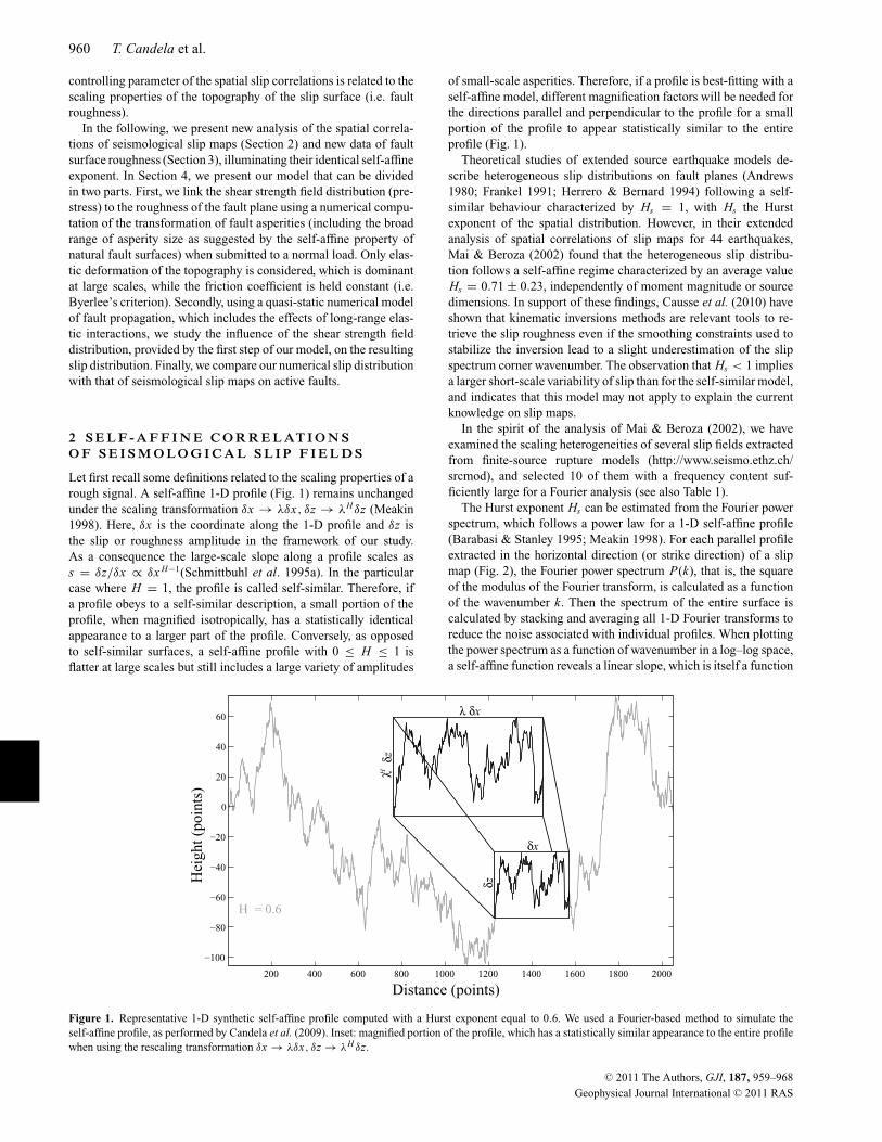
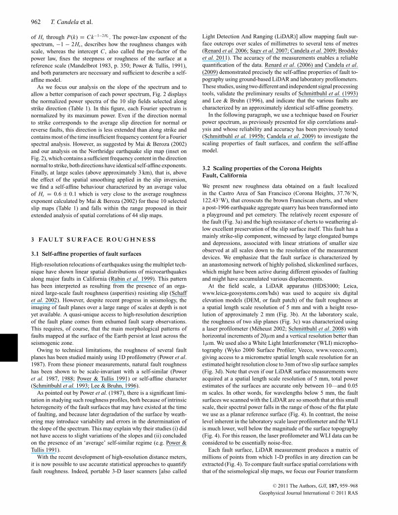
Let first recall some definitions related to the scaling properties of arough signal. A self-affine 1-D profile (Fig. 1) remains unchangedunder the scaling transformation δx → λδx, δz → λH δz (Meakin1998). Here, δx is the coordinate along the 1-D profile and δz isthe slip or roughness amplitude in the framework of our study.As a consequence the large-scale slope along a profile scales ass = δz/δx ∝ δx H−1(Schmittbuhl et al. 1995a). In the particularcase where H = 1, the profile is called self-similar. Therefore, ifa profile obeys to a self-similar description, a small portion of theprofile, when magnified isotropically, has a statistically identicalappearance to a larger part of the profile. Conversely, as opposedto self-similar surfaces, a self-affine profile with 0 ≤ H ≤ 1 isflatter at large scales but still includes a large variety of amplitudes

of small-scale asperities. Therefore, if a profile is best-fitting with aself-affine model, different magnification factors will be needed forthe directions parallel and perpendicular to the profile for a smallportion of the profile to appear statistically similar to the entireprofile (Fig. 1).

Theoretical studies of extended source earthquake models de-scribe heterogeneous slip distributions on fault planes (Andrews1980; Frankel 1991; Herrero & Bernard 1994) following a self-similar behaviour characterized by Hs = 1, with Hs the Hurstexponent of the spatial distribution. However, in their extendedanalysis of spatial correlations of slip maps for 44 earthquakes,Mai & Beroza (2002) found that the heterogeneous slip distribu-tion follows a self-affine regime characterized by an average valueHs = 0.71 ± 0.23, independently of moment magnitude or sourcedimensions. In support of these findings, Causse et al. (2010) haveshown that kinematic inversions methods are relevant tools to re-trieve the slip roughness even if the smoothing constraints used tostabilize the inversion lead to a slight underestimation of the slipspectrum corner wavenumber. The observation that Hs < 1 impliesa larger short-scale variability of slip than for the self-similar model,and indicates that this model may not apply to explain the currentknowledge on slip maps.

In the spirit of the analysis of Mai & Beroza (2002), we haveexamined the scaling heterogeneities of several slip fields extractedfrom finite-source rupture models (http://www.seismo.ethz.ch/srcmod), and selected 10 of them with a frequency content suf-ficiently large for a Fourier analysis (see also Table 1).

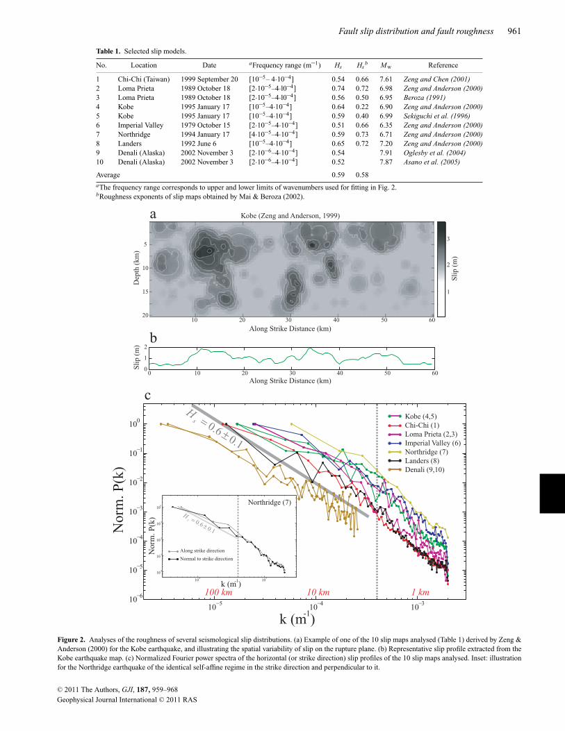
The Hurst exponent Hs can be estimated from the Fourier powerspectrum, which follows a power law for a 1-D self-affine profile(Barabasi & Stanley 1995; Meakin 1998). For each parallel profileextracted in the horizontal direction (or strike direction) of a slipmap (Fig. 2), the Fourier power spectrum P(k), that is, the squareof the modulus of the Fourier transform, is calculated as a functionof the wavenumber k. Then the spectrum of the entire surface iscalculated by stacking and averaging all 1-D Fourier transforms toreduce the noise associated with individual profiles. When plottingthe power spectrum as a function of wavenumber in a log–log space,a self-affine function reveals a linear slope, which is itself a function

200 400 600 800 1000 1200 1400 1600 1800 2000

0

20

40

60

Distance (points)

Hei

ght (

poin

ts)

λ δx

δz

δx

λ δ

zH

H = 0.6

Figure 1. Representative 1-D synthetic self-affine profile computed with a Hurst exponent equal to 0.6. We used a Fourier-based method to simulate theself-affine profile, as performed by Candela et al. (2009). Inset: magnified portion of the profile, which has a statistically similar appearance to the entire profilewhen using the rescaling transformation δx → λδx, δz → λH δz.

C© 2011 The Authors, GJI, 187, 959–968

Geophysical Journal International C© 2011 RAS

Fault slip distribution and fault roughness 961

Table 1. Selected slip models.

No. Location Date aFrequency range (m–1) Hs Hsb Mw Reference

1 Chi-Chi (Taiwan) 1999 September 20 [10–5– 4·10–4] 0.54 0.66 7.61 Zeng and Chen (2001)2 Loma Prieta 1989 October 18 [2·10–5–4·l0–4] 0.74 0.72 6.98 Zeng and Anderson (2000)3 Loma Prieta 1989 October 18 [2·10–5–4·l0–4] 0.56 0.50 6.95 Beroza (1991)4 Kobe 1995 January 17 [10–5–4·10–4] 0.64 0.22 6.90 Zeng and Anderson (2000)5 Kobe 1995 January 17 [10–5–4·10–4] 0.59 0.40 6.99 Sekiguchi et al. (1996)6 Imperial Valley 1979 October 15 [2·10–5–4·10–4] 0.51 0.66 6.35 Zeng and Anderson (2000)7 Northridge 1994 January 17 [4·10–5–4·10–4] 0.59 0.73 6.71 Zeng and Anderson (2000)8 Landers 1992 June 6 [10–5–4·10–4] 0.65 0.72 7.20 Zeng and Anderson (2000)9 Denali (Alaska) 2002 November 3 [2·10–6–4·10–4] 0.54 7.91 Oglesby et al. (2004)10 Denali (Alaska) 2002 November 3 [2·10–6–4·10–4] 0.52 7.87 Asano et al. (2005)

Average 0.59 0.58aThe frequency range corresponds to upper and lower limits of wavenumbers used for fitting in Fig. 2.bRoughness exponents of slip maps obtained by Mai & Beroza (2002).

Figure 2. Analyses of the roughness of several seismological slip distributions. (a) Example of one of the 10 slip maps analysed (Table 1) derived by Zeng &Anderson (2000) for the Kobe earthquake, and illustrating the spatial variability of slip on the rupture plane. (b) Representative slip profile extracted from theKobe earthquake map. (c) Normalized Fourier power spectra of the horizontal (or strike direction) slip profiles of the 10 slip maps analysed. Inset: illustrationfor the Northridge earthquake of the identical self-affine regime in the strike direction and perpendicular to it.

C© 2011 The Authors, GJI, 187, 959–968

Geophysical Journal International C© 2011 RAS

962 T. Candela et al.

of Hs through P(k) = Ck−1−2Hs . The power-law exponent of thespectrum, −1 − 2Hs , describes how the roughness changes withscale, whereas the intercept C , also called the pre-factor of thepower law, fixes the steepness or roughness of the surface at areference scale (Mandelbrot 1983, p. 350; Power & Tullis, 1991),and both parameters are necessary and sufficient to describe a self-affine model.

As we focus our analysis on the slope of the spectrum and toallow a better comparison of each power spectrum, Fig. 2 displaysthe normalized power spectra of the 10 slip fields selected alongstrike direction (Table 1). In this figure, each Fourier spectrum isnormalized by its maximum power. Even if the direction normalto strike corresponds to the average slip direction for normal orreverse faults, this direction is less extended than along strike andcontains most of the time insufficient frequency content for a Fourierspectral analysis. However, as suggested by Mai & Beroza (2002)and our analysis on the Northridge earthquake slip map (inset onFig. 2), which contains a sufficient frequency content in the directionnormal to strike, both directions have identical self-affine exponents.Finally, at large scales (above approximately 3 km), that is, abovethe effect of the spatial smoothing applied in the slip inversion,we find a self-affine behaviour characterized by an average valueof Hs = 0.6 ± 0.1 which is very close to the average roughnessexponent calculated by Mai & Beroza (2002) for these 10 selectedslip maps (Table 1) and falls within the range proposed in theirextended analysis of spatial correlations of 44 slip maps.

3 FAU LT S U R FA C E RO U G H N E S S

3.1 Self-affine properties of fault surfaces

High-resolution relocations of earthquakes using the multiplet tech-nique have shown linear spatial distributions of microearthquakesalong major faults in California (Rubin et al. 1999). This patternhas been interpreted as resulting from the presence of an orga-nized large-scale fault roughness (asperities) resisting slip (Schaffet al. 2002). However, despite recent progress in seismology, theimaging of fault planes over a large range of scales at depth is notyet available. A quasi-unique access to high-resolution descriptionof the fault plane comes from exhumed fault scarp observations.This requires, of course, that the main morphological patterns offaults mapped at the surface of the Earth persist at least across theseismogenic zone.

Owing to technical limitations, the roughness of several faultplanes has been studied mainly using 1D profilometry (Power et al.1987). From these pioneer measurements, natural fault roughnesshas been shown to be scale-invariant with a self-similar (Poweret al. 1987, 1988; Power & Tullis 1991) or self-affine character(Schmittbuhl et al. 1993; Lee & Bruhn, 1996).

As pointed out by Power et al. (1987), there is a significant limi-tation in studying such roughness profiles, both because of intrinsicheterogeneity of the fault surfaces that may have existed at the timeof faulting, and because later degradation of the surface by weath-ering may introduce variability and errors in the determination ofthe slope of the spectrum. This may explain why their studies (i) didnot have access to slight variations of the slopes and (ii) concludedon the presence of an ‘average’ self-similar regime (e.g. Power &Tullis 1991).

With the recent development of high-resolution distance meters,it is now possible to use accurate statistical approaches to quantifyfault roughness. Indeed, portable 3-D laser scanners [also called

Light Detection And Ranging (LiDAR)] allow mapping fault sur-face outcrops over scales of millimetres to several tens of metres(Renard et al. 2006; Sagy et al. 2007; Candela et al. 2009; Brodskyet al. 2011). The accuracy of the measurements enables a reliablequantification of the data. Renard et al. (2006) and Candela et al.(2009) demonstrated precisely the self-affine properties of fault to-pography using ground-based LiDAR and laboratory profilometers.These studies, using two different and independent signal processingtools, validate the preliminary results of Schmittbuhl et al. (1993)and Lee & Bruhn (1996), and indicate that the various faults arecharacterized by an approximately identical self-affine geometry.

In the following paragraph, we use a technique based on Fourierpower spectrum, as previously presented for slip correlations anal-ysis and whose reliability and accuracy has been previously tested(Schmittbuhl et al. 1995b; Candela et al. 2009) to investigate thescaling properties of fault surfaces, and confirm the self-affinemodel.

3.2 Scaling properties of the Corona HeightsFault, California

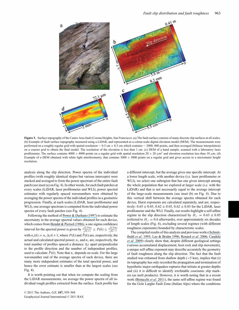
We present new roughness data obtained on a fault localizedin the Castro Area of San Francisco (Corona Heights, 37.76◦N,122.43◦W), that crosscuts the brown Franciscan cherts, and wherea post-1906 earthquake aggregate quarry has been transformed intoa playground and pet cemetery. The relatively recent exposure ofthe fault (Fig. 3a) and the high resistance of cherts to weathering al-low excellent preservation of the slip surface itself. This fault has amainly strike-slip component, witnessed by large elongated bumpsand depressions, associated with linear striations of smaller sizeobserved at all scales down to the resolution of the measurementdevices. We emphasize that the fault surface is characterized byan anastomosing network of highly polished, slickenlined surfaces,which might have been active during different episodes of faultingand might have accumulated various displacements.

At the field scale, a LiDAR apparatus (HDS3000; Leica,www.leica-geosystems.com/hds) was used to acquire six digitalelevation models (DEM, or fault patch) of the fault roughness ata spatial length scale resolution of 5 mm and with a height reso-lution of approximately 2 mm (Fig. 3b). At the laboratory scale,the roughness of two slip planes (Fig. 3c) was characterized usinga laser profilometer (Meheust 2002; Schmittbuhl et al. 2008) withhorizontal increments of 20μm and a vertical resolution better than1μm. We used also a White Light Interferometer (WLI) micropho-tography (Wyko 2000 Surface Profiler; Veeco, www.veeco.com),giving access to a micrometre spatial length scale resolution for anestimated height resolution close to 3nm of two slip surface samples(Fig. 3d). Note that even if our LiDAR surface measurements wereacquired at a spatial length scale resolution of 5 mm, total powerestimates of the surfaces are accurate only between 10—and 0.05m scales. In other words, for wavelengths below 5 mm, the faultsurfaces we scanned with the LiDAR are so smooth that at this smallscale, their spectral power falls in the range of those of the flat platewe use as a planar reference surface (Fig. 4). In contrast, the noiselevel inherent in the laboratory scale laser profilometer and the WLIis much lower, well below the magnitude of the surface topography(Fig. 4). For this reason, the laser profilometer and WLI data can beconsidered to be essentially noise-free.

Each fault surface, LiDAR measurement produces a matrix ofmillions of points from which 1-D profiles in any direction can beextracted (Fig. 4). To compare fault surface spatial correlations withthat of the seismological slip maps, we focus our Fourier transform

C© 2011 The Authors, GJI, 187, 959–968

Geophysical Journal International C© 2011 RAS

Fault slip distribution and fault roughness 963

Figure 3. Surface topography of the Castro Area fault (Corona Heights, San Francisco). (a) The fault surface consists of many discrete slip surfaces at all scales.(b) Example of fault surface topography measured using a LiDAR, and represented as a colour-scale digital elevation model (DEM). The measurements wereperformed on a roughly regular grid with spatial resolution ∼ 0.5 cm × 0.5 cm,which contains ∼ 2000, 000 points, and then averaged (bilinear interpolation)on a coarser grid to obtain the final model. The resolution of the elevation is less than 1 cm. (c) DEM of a hand sample, scanned with a laboratory laserprofilometer. The surface contains 4000 × 4000 points on a regular grid with spatial resolution 20 × 20 μm2 and elevation resolution less than 10 μm. (d)Example of a DEM obtained with white light interferometry, that contains 3000 × 3000 points on a regular grid and gives access to a micrometer heightresolution.

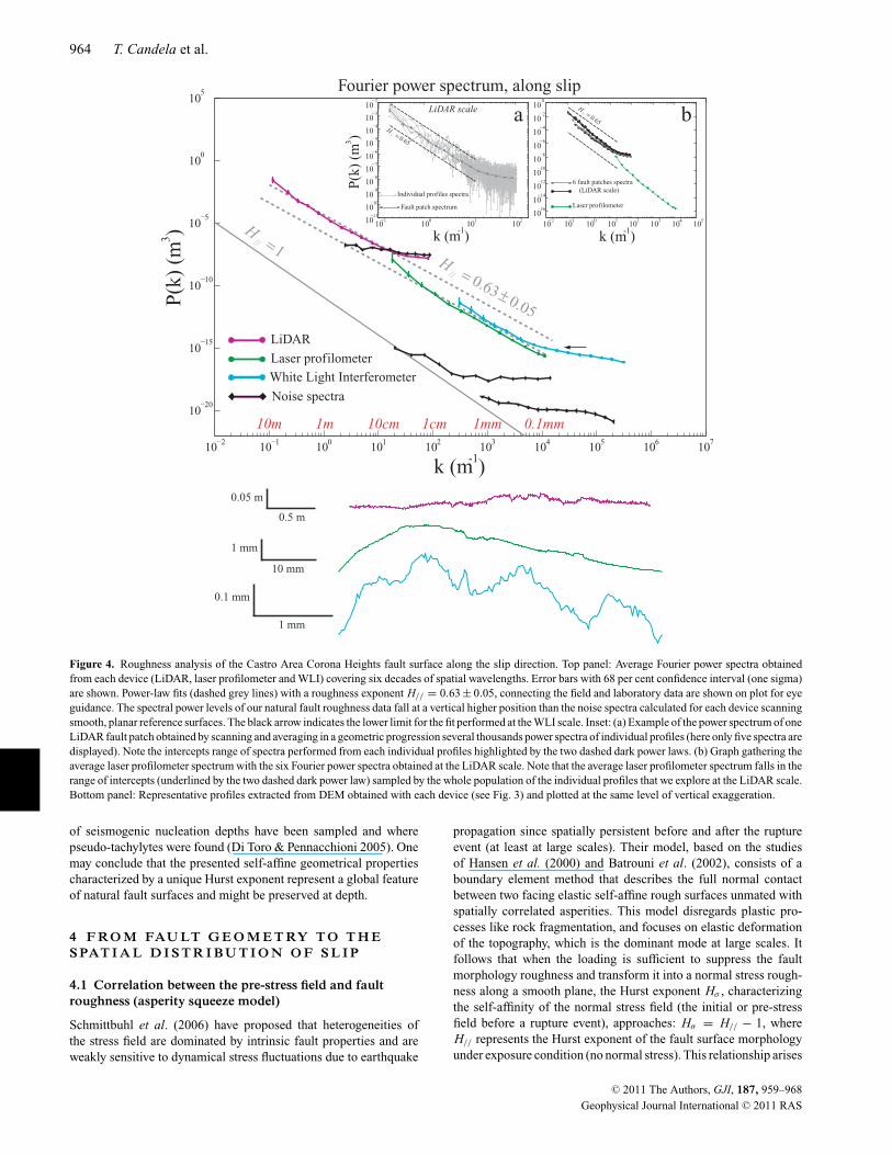
analysis along the slip direction. Power spectra of the individualprofiles (with roughly identical slopes but various intercepts) werestacked and averaged to form the power spectrum of the entire faultpatch (see inset (a) on Fig. 4). In other words, for each fault patches atevery scales (LiDAR, laser profilometer and WLI), power spectralestimates with regularly spaced wavenumbers were obtained byaveraging the power spectra of the individual profiles in a geometricprogression. Finally, at each scales (LiDAR, laser profilometer andWLI), one average spectrum is computed from the individual powerspectra of every fault patches (see Fig. 4).

Following the method of Power & Durham (1997) to estimate theuncertainty in the average spectral values obtained for each device,which comes from Bendat & Piersol (1986), a one sigma confidence

interval for the spectral power is given by√

ns P(k)√ns+1 ≤ P(k) ≤

√ns P(k)√ns−1

with ns(k) = ny�yk +1, where P(k) and P(k) are, respectively, theactual and calculated spectral power; ny and ns are, respectively, thetotal number of profiles spaced a distance �y apart perpendicularto the profile direction and the number of independent profiles,used to calculate P(k). Note that ns depends on scale. For the largewavenumber end of the average spectra of each device, there aremany more independent estimates of the total spectral power, andhence the error estimate is smaller than at the largest scales (seeFig. 4).

It is worth pointing out that when we compute the scaling fromthe LiDAR measurements, we average the power spectra of all in-dividual rough profiles extracted from the surface. Each profile has

a different intercept, but the average gives one specific intercept. Ata lower length scale, with another device (i.e. laser profilometer orWLI), we select one subregion that has one given intercept amongthe whole population that we explored at larger scale (i.e. with theLiDAR) and that is not necessarily equal to the average interceptof the large-scale measurements (see inset (b) on Fig. 4). Due tothis vertical shift between the average spectra obtained for eachdevice, Hurst exponents are calculated separately, and are, respec-tively: 0.65 ± 0.05, 0.62 ± 0.05, 0.62 ± 0.03 for the LiDAR, laserprofilometer and the WLI. Finally, our results highlight a self-affineregime in the slip direction characterized by H// = 0.63 ± 0.05(referred to H// = 0.6 afterwards), over approximately six decadesof length scales (Fig. 4), excluding several regimes (with differentroughness exponents) bounded by characteristic scales.

The compiled results of this analysis and previous works (Schmit-tbuhl et al. 1993; Lee & Bruhn 1996; Renard et al. 2006; Candelaet al. 2009) clearly show that, despite different geological settings(various accumulated displacement, host rock and slip movement),a unique self-affine exponent may describe accurately the geometryof fault roughness along the slip direction. The fact that the faultstudied was exhumed from shallow depth (<5 km), implies that (i)its topography has only recorded the propagation and termination ofhypothetic major earthquakes ruptures that initiate at greater depthsand (ii) it is difficult to identify irrefutable coseismic slip mark-ers (as melt products). However, it is worth noting that in a recentwork (Bistacchi et al. 2011), the same self-affine regime was foundfor the Gole Larghe Fault Zone (Italian Alps) where the conditions

C© 2011 The Authors, GJI, 187, 959–968

Geophysical Journal International C© 2011 RAS

964 T. Candela et al.

1// =

H

05.063.0//

±=

H

10 100

101

10210

11

1010

109

108

107

106

105

104

103

102

10 101

100

101

102

103

104

105

1016

1014

1012

1010

108

106

104

102

100

10 10 1 100 101 102 103 104 105 106 107

1020

1015

1010

105

100

105

10m 1m 10cm 1cm 1mm 0.1mm

P(k

) (m

)3

k (m )-1

P(k

) (m

)3

k (m )-1k (m )-1

a b

LiDAR

Laser profilometer

White Light Interferometer

Noise spectra

0.05 m

0.5 m

1 mm

10 mm

1 mm

0.1 mm

65.0// =

H

65.0// =

H

Individual profiles spectra

Fault patch spectrum

Fourier power spectrum, along slipLiDAR scale

6 fault patches spectra (LiDAR scale)

Laser profilometer

Figure 4. Roughness analysis of the Castro Area Corona Heights fault surface along the slip direction. Top panel: Average Fourier power spectra obtainedfrom each device (LiDAR, laser profilometer and WLI) covering six decades of spatial wavelengths. Error bars with 68 per cent confidence interval (one sigma)are shown. Power-law fits (dashed grey lines) with a roughness exponent H// = 0.63 ± 0.05, connecting the field and laboratory data are shown on plot for eyeguidance. The spectral power levels of our natural fault roughness data fall at a vertical higher position than the noise spectra calculated for each device scanningsmooth, planar reference surfaces. The black arrow indicates the lower limit for the fit performed at the WLI scale. Inset: (a) Example of the power spectrum of oneLiDAR fault patch obtained by scanning and averaging in a geometric progression several thousands power spectra of individual profiles (here only five spectra aredisplayed). Note the intercepts range of spectra performed from each individual profiles highlighted by the two dashed dark power laws. (b) Graph gathering theaverage laser profilometer spectrum with the six Fourier power spectra obtained at the LiDAR scale. Note that the average laser profilometer spectrum falls in therange of intercepts (underlined by the two dashed dark power law) sampled by the whole population of the individual profiles that we explore at the LiDAR scale.Bottom panel: Representative profiles extracted from DEM obtained with each device (see Fig. 3) and plotted at the same level of vertical exaggeration.

of seismogenic nucleation depths have been sampled and wherepseudo-tachylytes were found (Di Toro & Pennacchioni 2005). Onemay conclude that the presented self-affine geometrical propertiescharacterized by a unique Hurst exponent represent a global featureof natural fault surfaces and might be preserved at depth.

4 F RO M FAU LT G E O M E T RY T O T H ES PAT I A L D I S T R I B U T I O N O F S L I P

4.1 Correlation between the pre-stress field and faultroughness (asperity squeeze model)

Schmittbuhl et al. (2006) have proposed that heterogeneities ofthe stress field are dominated by intrinsic fault properties and areweakly sensitive to dynamical stress fluctuations due to earthquake

propagation since spatially persistent before and after the ruptureevent (at least at large scales). Their model, based on the studiesof Hansen et al. (2000) and Batrouni et al. (2002), consists of aboundary element method that describes the full normal contactbetween two facing elastic self-affine rough surfaces unmated withspatially correlated asperities. This model disregards plastic pro-cesses like rock fragmentation, and focuses on elastic deformationof the topography, which is the dominant mode at large scales. Itfollows that when the loading is sufficient to suppress the faultmorphology roughness and transform it into a normal stress rough-ness along a smooth plane, the Hurst exponent Hσ , characterizingthe self-affinity of the normal stress field (the initial or pre-stressfield before a rupture event), approaches: Hσ = H// − 1, whereH// represents the Hurst exponent of the fault surface morphologyunder exposure condition (no normal stress). This relationship arises

C© 2011 The Authors, GJI, 187, 959–968

Geophysical Journal International C© 2011 RAS

Fault slip distribution and fault roughness 965

from the fact that, for an elastic material, the stress field is relatedto the first derivative of the displacement field. If we use our es-timate of the Hurst exponent of the fault morphology H// = 0.6,we obtain that the Hurst exponent of the normal stress field is:Hσ = −0.4.

4.2 A quasi-static heterogeneous slip distribution model

We use a quasi-static 3-D fault model, detailed by Perfettini et al.(2001), which accounts for long-range elastic interactions. Perfettiniet al. (2001) have examined the influence of spatial heterogeneitiesof frictional strength on the slip distribution along a creeping fault.In this model, slip fluctuates spatially because of pinning on localasperities (heterogeneities of frictional strength). Depinning fromthese asperities involves local instabilities. When the elastic cou-pling is small, the motion is controlled by individual asperities.Conversely, for strong elastic coupling, that is, weak pinning, as-perities interact because of elasticity and the dynamics becomesglobal.

In distinction to the study of Perfettini et al. (2001), where auniform random distribution of frictional strength was used to char-acterize a heterogeneous static pre-stress field, we consider here,also a disorder of the frictional strength (or shear strength) but spa-tially correlated and controlled by a self-affine exponent Hτ . Wepropose to link the Hurst exponent of the shear strength Hτ to thatof the normal stress Hσ on the basis of a local Byerlee criterion:τc = μσn with μ = 0.6. Because of the linearity between the shearstrength and the normal stress, both are expected to exhibit thesame scaling leading to: Hτ = Hσ = H// − 1. With our estimate ofH// = 0.6, we obtainHτ = −0.4.

4.2.1 Numerical model

In this paragraph, we briefly list the main characteristics and as-sumptions of the quasi-static numerical fault model, based on thestudy of Perfettini et al. (2001). We consider a simple elastic modelof rupture along a fault plane located at z = 0 through an un-bounded homogeneous elastic solid. The rupture propagates alongthe y direction.

The problem is then governed by a quasi-static scalar wave equa-tion involving a 2-D displacement field U (x, z; t), and the relatedshear traction across planes parallel to the crack is σ (x, z; t). The ac-tual slip u(x ; t) = U (x, 0+; t) −U (x, 0−; t) is the slip discontinuityacross the fault plane and τ (x ; t) denotes the associated perturbationof traction. We assume that slip occurs quasi-statically and neglectany dynamical effects. In that case, elastic waves are neglected, andthe stress change τ (x ; t), located at y = 0, and due to variations ofslip discontinuity along the fault is given by (e.g. Cochard & Rice1997)

τ (x ; t) = G

2πPV

∫L

J (x − ξ )[u(ξ ; t) − u(x ; t)] dξ, (1)

where integration takes place over the fault of size L andPV indicates the principal value. The elastic kernel J (x) = 1/x2

accounts for the long-range elastic interactions and G is the shearmodulus. To avoid edge effects, we assume an L-periodic interfacein the x direction such that the 1/x2 kernel in (1) transforms inJL (x) = (π/L)2/ sin2(πx/L).

To characterize locally the heterogeneous frictional propertiesalong the interface, we balance τ (x ; t) with a frictional strengththat does not evolve with time ηp(x ; u(x ; t)). To mimic the spa-tial heterogeneities of the frictional strength previously described,

their fluctuations are assumed to be spatially correlated with long-range correlations, that is, the frictional strength are controlled bya negative self-affine exponent Hτ = −0.4. A uniform randomdistribution of the frictional strength (Perfettini et al. 2001) wouldcorrespond to Hτ = −1 in two dimensions (Hansen et al. 2001). Thecorrelation function of the frictional strength is assumed to behaveas (x − x ′) ∝ |(x − x ′)|2Hτ and in Fourier space P(k) ∝ k−2−2Hτ .

At any time, the quasi-static motion of the fault has to satisfy:ηp(x ; u(x ; t)) ≥ τ (x ; t) for all points of the interface. The evolutionof the system may be regarded as purely dissipative, that is, all thereleased energy being dissipated by frictional work (Fisher 1998).

The loading results from an imposed displacement. The systemis discretized both in time and space. An elementary step (i.e. atime step) corresponds to the motion of only one segment for whicha frictional strength ηp(x ; u(x ; t)) has been defined. At each step,the weakest segment is searched for (i.e. event-driven dynamics)by assuming that its location corresponds to the least shear tractionrequired to advance the crack and slips by an elementary distancewhich is a fraction of the discretization length. The local drivingforce is locally updated according to the adopted self-affine distri-bution to follow the imposed disorder of the frictional strength. Atthat stage, the rupture front is locally unloaded and all the forcesalong the front line are modified according to a discretized form ofeq. (1). The procedure is then repeated. The behaviour of the systemis controlled by the competition between local fluctuations of thefrictional strength and the effects of long-range elastics interactions.

Perfettini et al. (2001) have shown that three regimes of slipcorrelations exist depending on the ratio of the stress drop of apoint that just slipped by an elementary distance and the root-mean-square (rms) of the frictional strength fluctuations. In thefirst regime, when the stress drop is much greater than the rmsof the frictional strength fluctuations, the heterogeneities are notstrong enough to pin the front, thus crack advance can never bearrested. Conversely, slip in the second regime is expected to havethe same statistical distribution as the fluctuation of the frictionalstrength, because the magnitude of the elastic interactions (due toa small stress drop) is much smaller than the frictional strengthheterogeneities. The third regime, on which we focus our study, isintermediate and the magnitude of the elastic interactions is compa-rable to the frictional strength variations. The interactions betweenfrictional strength heterogeneities and elastic stress transfers lead tonon-trivial spatio-temporal correlations of slips.

4.2.2 Results

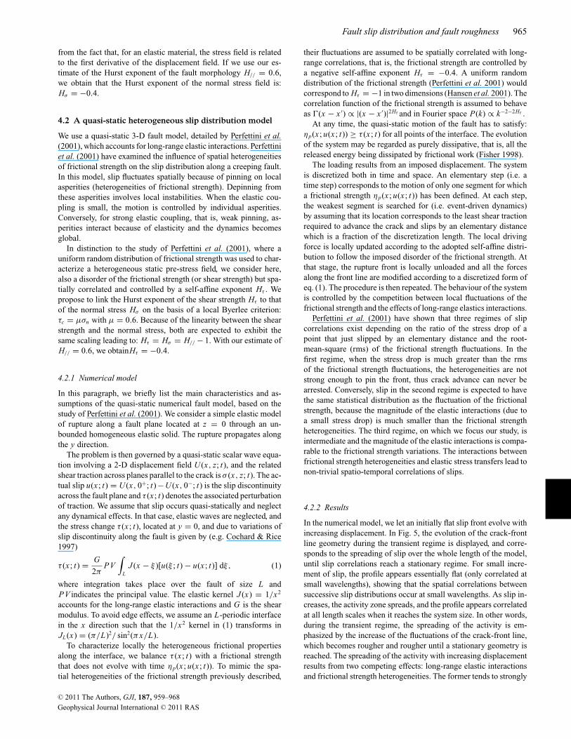
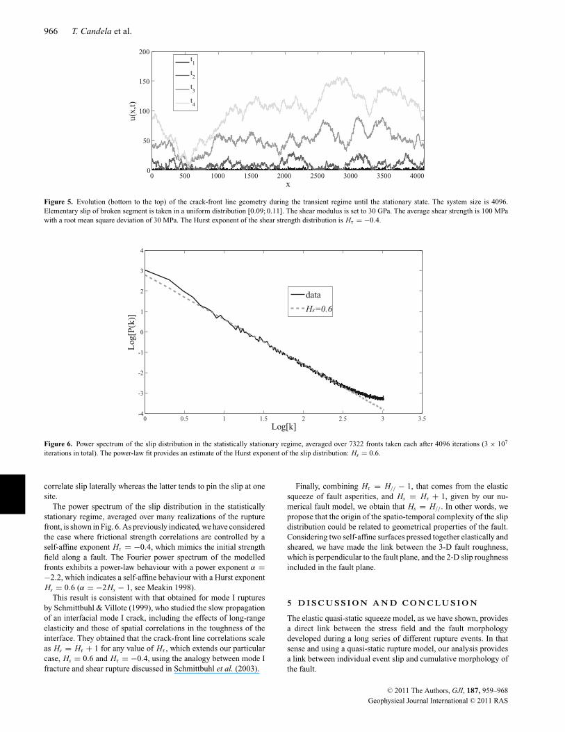
In the numerical model, we let an initially flat slip front evolve withincreasing displacement. In Fig. 5, the evolution of the crack-frontline geometry during the transient regime is displayed, and corre-sponds to the spreading of slip over the whole length of the model,until slip correlations reach a stationary regime. For small incre-ment of slip, the profile appears essentially flat (only correlated atsmall wavelengths), showing that the spatial correlations betweensuccessive slip distributions occur at small wavelengths. As slip in-creases, the activity zone spreads, and the profile appears correlatedat all length scales when it reaches the system size. In other words,during the transient regime, the spreading of the activity is em-phasized by the increase of the fluctuations of the crack-front line,which becomes rougher and rougher until a stationary geometry isreached. The spreading of the activity with increasing displacementresults from two competing effects: long-range elastic interactionsand frictional strength heterogeneities. The former tends to strongly

C© 2011 The Authors, GJI, 187, 959–968

Geophysical Journal International C© 2011 RAS

966 T. Candela et al.

0 500 1000 1500 2000 2500 3000 3500 40000

50

100

150

200

x

u(x,

t)

t1

t2

t3

t4

Figure 5. Evolution (bottom to the top) of the crack-front line geometry during the transient regime until the stationary state. The system size is 4096.Elementary slip of broken segment is taken in a uniform distribution [0.09; 0.11]. The shear modulus is set to 30 GPa. The average shear strength is 100 MPawith a root mean square deviation of 30 MPa. The Hurst exponent of the shear strength distribution is Hτ = −0.4.

0 0.5 1 1.5 2 2.5 3 3.5-4

-3

-2

-1

0

1

2

3

4

Log[k]

Log

[P(k

)]

data

Hs=0.6

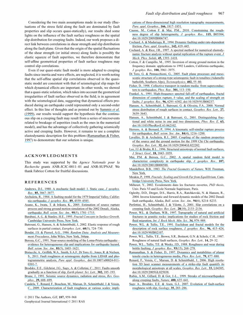
Figure 6. Power spectrum of the slip distribution in the statistically stationary regime, averaged over 7322 fronts taken each after 4096 iterations (3 × 107

iterations in total). The power-law fit provides an estimate of the Hurst exponent of the slip distribution: Hs = 0.6.

correlate slip laterally whereas the latter tends to pin the slip at onesite.

The power spectrum of the slip distribution in the statisticallystationary regime, averaged over many realizations of the rupturefront, is shown in Fig. 6. As previously indicated, we have consideredthe case where frictional strength correlations are controlled by aself-affine exponent Hτ = −0.4, which mimics the initial strengthfield along a fault. The Fourier power spectrum of the modelledfronts exhibits a power-law behaviour with a power exponent α =−2.2, which indicates a self-affine behaviour with a Hurst exponentHs = 0.6 (α = −2Hs − 1, see Meakin 1998).

This result is consistent with that obtained for mode I rupturesby Schmittbuhl & Villote (1999), who studied the slow propagationof an interfacial mode I crack, including the effects of long-rangeelasticity and those of spatial correlations in the toughness of theinterface. They obtained that the crack-front line correlations scaleas Hs = Hτ + 1 for any value of Hτ , which extends our particularcase, Hs = 0.6 and Hτ = −0.4, using the analogy between mode Ifracture and shear rupture discussed in Schmittbuhl et al. (2003).

Finally, combining Hτ = H// − 1, that comes from the elasticsqueeze of fault asperities, and Hs = Hτ + 1, given by our nu-merical fault model, we obtain that Hs = H//. In other words, wepropose that the origin of the spatio-temporal complexity of the slipdistribution could be related to geometrical properties of the fault.Considering two self-affine surfaces pressed together elastically andsheared, we have made the link between the 3-D fault roughness,which is perpendicular to the fault plane, and the 2-D slip roughnessincluded in the fault plane.

5 D I S C U S S I O N A N D C O N C LU S I O N

The elastic quasi-static squeeze model, as we have shown, providesa direct link between the stress field and the fault morphologydeveloped during a long series of different rupture events. In thatsense and using a quasi-static rupture model, our analysis providesa link between individual event slip and cumulative morphology ofthe fault.

C© 2011 The Authors, GJI, 187, 959–968

Geophysical Journal International C© 2011 RAS

Fault slip distribution and fault roughness 967

Considering the two main assumptions made in our study (fluc-tuations of the stress field along the fault are dominated by faultproperties and slip occurs quasi-statically), our results shed somelights on the influence of the fault surface roughness on the spatialslip distribution for creeping faults. Indeed, our work proposes a di-rect link between correlations in shear strength and slip distributionalong the fault plane. Given that the origin of the spatial fluctuationsof the shear strength (or initial stress) along faults is possibly theelastic squeeze of fault asperities, we therefore demonstrate thatself-affine geometrical properties of fault surface roughness maycontrol slip correlations.

Even if our quasi-static fault model is more adapted to creepingfaults since inertia and wave effects, are neglected, it is worth notingthat the self-affine spatial slip correlations observed in the quasi-static model are consistent with that of seismological slip maps forwhich dynamical effects are important. In other words, we showedthat a quasi-static solution, which takes into account the geometricalirregularities of fault surface observed in the field, is in agreementwith the seismological data, suggesting that dynamical effects pro-duced during an earthquake could represented only a second-ordereffect. In this line of thoughts and as pointed out by Sammis et al.(1999), our results would support the hypothesis that the continu-ous slip on a creeping fault may result from a series of microeventsrelated to breakage of asperities (such as the ones in the numericalmodel), and has the advantage of collectively gathering seismicallyactive and creeping faults. However, it remains to use a completeelastodynamic description for this problem (Ramanathan & Fisher,1997) to demonstrate that our solution is unique.

A C K N OW L E D G M E N T S

This study was supported by the Agence Nationale pour laRecherche grants ANR-JCJC-0011–01 and ANR-SUPNAF. Wethank Fabrice Cotton for fruitful discussions.

R E F E R E N C E S

Andrews, D.J., 1980. A stochastic fault model: 1. Static case, J. geophys.Res., 85, 3867–3877.

Archuleta, R., 1984. A faulting model for the 1979 Imperial Valley, Califor-nia earthquake, J. geophys. Res., 89, 4559–4585.

Asano, K., Iwata, T. & Irikura, K., 2005. Estimation of source ruptureprocess and strong ground motion simulation of the 2002 Denali, Alaska,earthquake, Bull. seism. Soc. Am., 95(5), 1701–1715.

Barabasi, A.-L. & Stanley, H.E., 1995. Fractal Concepts in Surface Growth.Cambridge University Press, New York.

Batrouni, G., Hansen, A. & Schmittbuhl, J., 2002. Elastic response of roughsurfaces in partial contact, Europhys. Lett., 60(5), 724–730.

Bendat, J.S. & Piersol, A.G., 1986. Random Data: Analysis and Measure-ment Procedures, John Wiley, New York, 566pp.

Beroza, G.C., 1991. Near-source modeling of the Loma-Prieta earthquake –evidence for heterogeneous slip and implications for earthquake hazard,Bull. seism. Soc. Am., 81(5), 1603–1621.

Bistacchi, A., Griffith, W.A., Smith, S.A.F., Di Toro, G., Jones, R. & Nielsen,S., 2011. Fault roughness at seismogenic depths from LIDAR and pho-togrammetric analysis, Pure appl. Geophys., doi:10.1007/s00024-011-0301-7.

Brodsky, E.E., Gilchrist, J.G., Sagy, A. & Colletini, C., 2011. Faults smoothgradually as a function of slip, Earth planet. Sci. Lett., 302, 185–193.

Brune, J., 1991. Seismic source dynamics, radiation and stress, Rev. Geo-phys., 29, 688–699.

Candela, T., Renard, F., Bouchon, M., Marsan, D., Schmittbuhl, J. & Voisin,C., 2009. Characterization of fault roughness at various scales: impli-

cations of three-dimensional high resolution topography measurements,Pure. appl. Geophys., 166, 1817–1851.

Causse, M., Cotton F. & Mai, P.M., 2010. Constraining the rough-ness degree of slip heterogeneity, J. geophys. Res., 115, B05304,doi:10.1029/2009JB006747.

Cochard, A. & Madariaga, R., 1994. Dynamic faulting under rate-dependentfriction, Pure. appl. Geophys., 142, 419–445.

Cochard, A. & Rice, J.R., 1997. A spectral method for numerical elastody-namic fracture analysis without spatial replication of the rupture event, J.Mech. Phys. Solids, 45, 1393–1418.

Cotton, F. & Campillo, M., 1995. Inversion of strong ground motion in thefrequency domain: applications to 1992 Landers, California earthquake,J. geophys. Res., 100, 3961–3975.

Di Toro, G. & Pennacchioni, G., 2005. Fault plane processes and meso-scopic structure of a strong-type seismogenic fault in tonalites (Adamellobatholith, Southern Alps), Tectonophysics, 402, 55–80.

Fisher, D., 1998. Collective transport in random media: from superconduc-tors to earthquakes, Phys. Rep., 301, 113–150.

Frankel, A., 1991. High-frequency spectral fall-off of earthquakes, fractaldimension of complex rupture, b value, and the scaling of strength onfaults, J. geophys. Res., 96, 6291–6302, doi:10.1029/91JB00237.

Hansen, A., Schmittbuhl, J., Batrouni, G. & Oliveira, F.A., 2000. Normalstress distribution of rough surfaces in contact, Geophys. Res. Lett., 27,3639–3643.

Hansen, A., Schmittbuhl, J. & Batrouni, G., 2001. Distinguishing frac-tional and white noise in one and two dimensions, Phys. Rev. E, 63,doi:10.1103/PhysRevE.63.062102.

Herrero, A. & Bernard, P., 1994. A kinematic self-similar rupture processfor earthquakes, Bull. seism. Soc. Am., 84(4), 1216–1288.

Lavallee, D. & Archuleta, R.J., 2005. Coupling of the random propertiesof the source and the ground motion for the 1999 Chi Chi earthquake,Geophys. Res. Lett., 32, doi:10.1029/2004GL022202.

Lee, J.J. & Bruhn, R.L., 1996. Structural anisotropy of normal fault surfaces,J. Struct. Geol., 18, 1043–1059.

Mai, P.M. & Beroza, G.C., 2002. A spatial random field model tocharacterize complexity in earthquake slip, J. geophys. Res., 107,doi:10.1029/2001JB000588.

Mandelbrot, B.B., 1983. The Fractal Geometry of Nature, W.H. Freeman,New York.

Meakin, P., 1998. Fractals: Scaling and Growth Far from Equilibrium, Cam-bridge University Press, New York.

Meheust, Y., 2002. Ecoulements dans les fractures ouvertes, PhD thesis,Univ. Paris VI and Ecole Normale Superieure, Paris.

Oglesby, D.D., Dreger, D.S., Harris, R.A., Ratchkovski, N. & Hansen, R.,2004. Inverse kinematic and forward dynamic models of the 2002 Denalifault earthquake, Alaska, Bull. seism. Soc. Am., 94(6), S214–S233.

Perfettini, H., Schmittbuhl, J. & Vilotte, J., 2001. Slip correlations on acreeping fault, Geophys. Res. Lett., 28(10), 2133–2136.

Power, W.L. & Durham, W.B., 1997. Topography of natural and artificialfractures in granitic rocks: implications for studies of rock friction andfluid migration, Int. J. Rock Mech. Min. Sci., 34, 979–989.

Power, W.L. & Tullis, T.E., 1991. Euclidean and fractal models for thedescription of rock surface roughness, J. geophys. Res., 96, 415–424,doi:10.1029/90JB02107.

Power, W.L., Tullis, T.E., Brown, S.R., Boitnott, G.N. & Scholz, C.H., 1987.Roughness of natural fault surfaces, Geophys. Res. Lett., 14, 29–32.

Power, W.L., Tullis, T.E. & Weeks, J.D., 1988. Roughness and wear duringbrittle faulting, J. geophys. Res., 93(15), 268–278.

Ramanathan, S. & Fisher, D., 1997. Dynamics and instabilities of planartensile cracks in heterogeneous media, Phys. Rev. Lett., 79, 877–880.

Renard, F., Voisin, C., Marsan, D. & Schmittbuhl, J., 2006. High resolu-tion 3D laser scanner measurements of a strike-slip fault quantify itsmorphological anisotropy at all scales, Geophys. Res. Lett., 33, L04305,doi:10.1029/2005GL025038.

Rubin, A.M., Gillard, D. & Got, J.-L., 1999. Streaks of microearthquakesalong creeping faults, Nature, 400, 635–641.

Sagy A., Brodsky, E.E. & Axen, G.J., 2007. Evolution of fault-surfaceroughness with slip, Geology, 35, 283–286.

C© 2011 The Authors, GJI, 187, 959–968

Geophysical Journal International C© 2011 RAS

968 T. Candela et al.

Sammis, C.G., Nadeau, R.M. & Johnson, L.R., 1999. How strong is an asper-ity? J. geophys. Res., 104, 10 609–10 619, doi:10.1029/1999JB900006.

Schaff, D.P., Bokelmann, G.H.R., Beroza, G.C., Waldhauser, F. & Ellsworth,W.L., 2002. High-resolution image of Calaveras fault seismicity, J. geo-phys. Res., 107, doi:10.1029/2001JB000633.

Schmittbuhl, J. & Vilotte, J., 1999. Interfacial crack front wandering: influ-ence of correlated quenched noise, Physica A, 270, 42–56.

Schmittbuhl, J., Gentier, S. & Roux, R., 1993. Field measurements of theroughness of fault surfaces, Geophys. Res. Lett., 20, 639–641.

Schmittbuhl, J., Schmitt, F. & Scholz, C.H., 1995a. Scaling invariance ofcrack surfaces, J. geophys. Res., 100, 5953–5973.

Schmittbuhl, J., Vilotte, J.P. & Roux, S., 1995b. Reliability of self-affinemeasurements, Phys. Rev. E, 51, 131–147.

Schmittbuhl, J., Delaplace, A., Maloy, K., Perfettini, H. & Vilotte, J., 2003.Slow crack propagation and slip correlations, Pure appl. Geophys., 160,961–976, doi:10.1007/PL00012575.

Schmittbuhl, J., Chambon, G., Hansen, A. & Bouchon, M., 2006. Are stressdistributions along faults the signature of asperity squeeze? Geophys. Res.Lett., 33, doi:10.1029/2006GL025952.

Schmittbuhl, J., Steyer, A., Jouniaux, L. & Toussaint, R., 2008. Fracture mor-phology and viscous transport, Int. J. Rock. Mech. Min. Sci., 45, 422–430.

Sekiguchi, H., Irikura, K., Iwata, T., Kakehi, Y. & Hoshiba, M., 1996.Minute locating of faulting beneath Kobe and the waveform inversion ofthe source process during the 1995 Hyogo-ken Nanbu, Japan, earthquakeusing strong ground motion records, J. Phys. Earth, 44(5), 473–487.

Zeng, Y. & Anderson, J., 2000. Evaluation of numerical proceduresfor simulating near-fault long-period ground motions using Zengmethod, Report 2000/01 to the PEER Utilities Program, available athttp://peer.berkeley.edu

Zeng, Y.H. & Chen, C.H., 2001. Fault rupture process of the 20 Septem-ber 1999 Chi-Chi, Taiwan, earthquake, Bull. seism. Soc. Am., 91(5),1088–1098.

C© 2011 The Authors, GJI, 187, 959–968

Geophysical Journal International C© 2011 RAS