Fault-slip analysis and paleostress reconstruction slip...1 Fault-slip analysis and paleostress reconstruction Definitions Faults have displacements parallel to the fault, visible

1

Fault-slip analysis and paleostress reconstruction Definitions Faults have displacements parallel to the fault, visible by naked eye. Faults bear slickenside lineations. Faults denote simple shear; pure dilatant veins and pressure-solution seams (stylolits) yield extension and compression directions. Record them. See Fig. 4.2, Fig. 4.4.

Fault-slip geometry of large faults is commonly inferred from observations of minor faults in neighboring outcrops, assuming that the mechanisms are similar, despite difference in size. Slip orientation is provided by slickenside lineations. Most fault surfaces are striated, and the attitude of the striae reveals the orientation of slip.

2

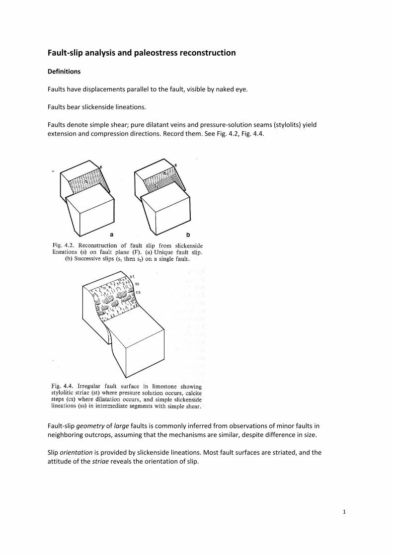
Fault geometry The geometry of a fault can be described at one point through the measurement of three angles and one distance (Fig. 4.11): (a) d, dip direction, 0-360° (b) p, dip of the fault plane, 0-90° (c) i, pitch of the slickenside lineations which indicates the slip direction; 0-360° and needs a sign convention. One proposal (Angelier): i is measured positive counterclockwise from the right side of the fault plane dipping towards the observer (d) distance of the fault displacement

3

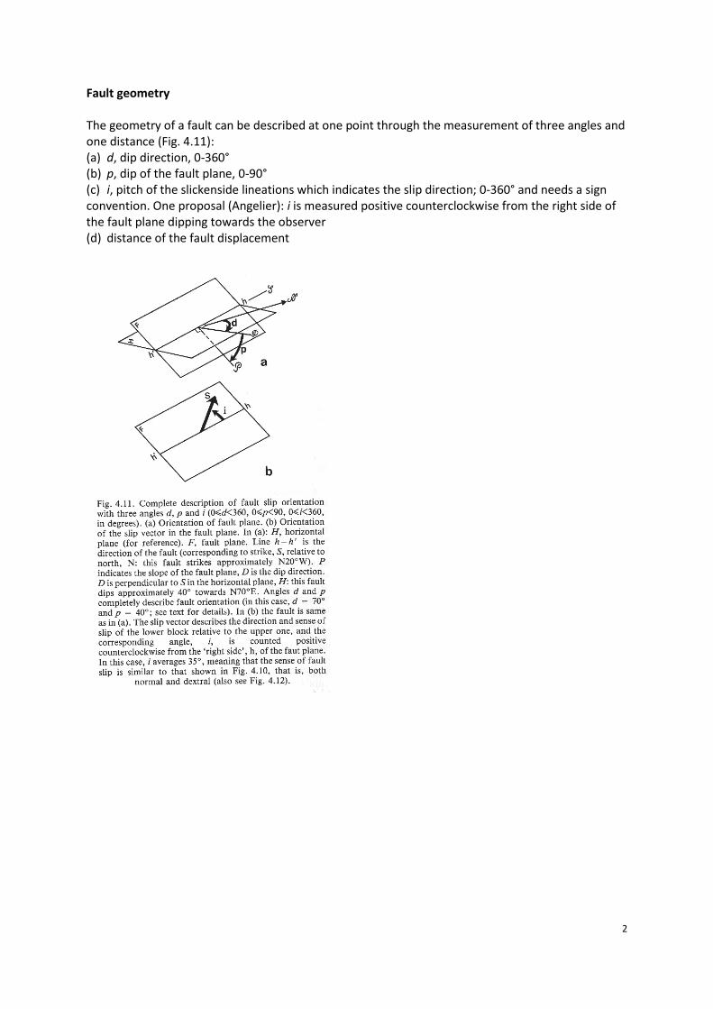
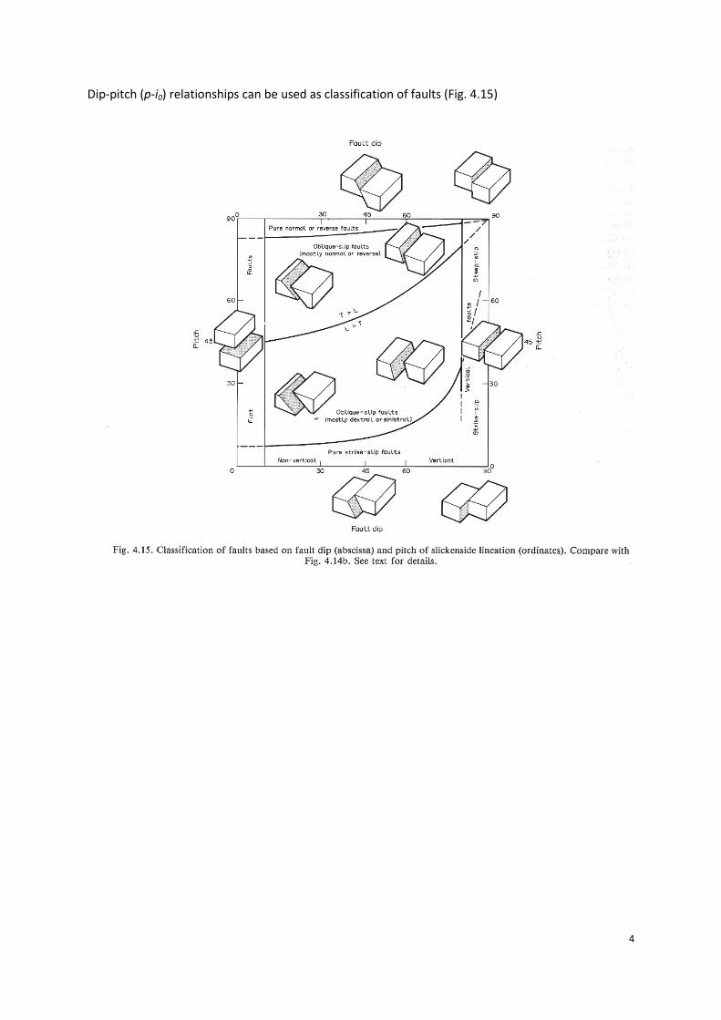
Components of fault displacement The various components of slip can be represented by a vector D (Fig. 4.13); if p and i0, now defined as pitch that ranges from 0 to 90° regardless of the sense, are measured, all possible vector components can be defined.

4

Dip-pitch (p-i0) relationships can be used as classification of faults (Fig. 4.15)

5

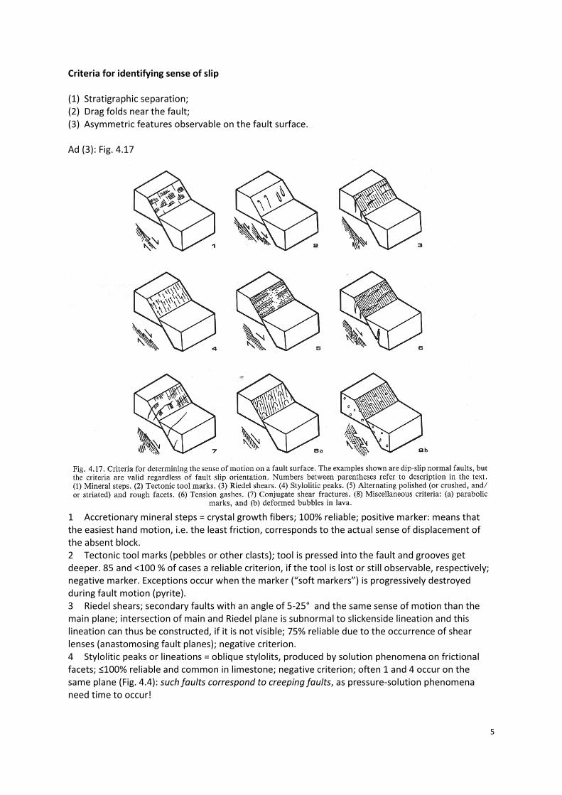
Criteria for identifying sense of slip (1) Stratigraphic separation; (2) Drag folds near the fault; (3) Asymmetric features observable on the fault surface. Ad (3): Fig. 4.17

1 Accretionary mineral steps = crystal growth fibers; 100% reliable; positive marker: means that the easiest hand motion, i.e. the least friction, corresponds to the actual sense of displacement of the absent block. 2 Tectonic tool marks (pebbles or other clasts); tool is pressed into the fault and grooves get deeper. 85 and <100 % of cases a reliable criterion, if the tool is lost or still observable, respectively; negative marker. Exceptions occur when the marker (“soft markers”) is progressively destroyed during fault motion (pyrite). 3 Riedel shears; secondary faults with an angle of 5-25° and the same sense of motion than the main plane; intersection of main and Riedel plane is subnormal to slickenside lineation and this lineation can thus be constructed, if it is not visible; 75% reliable due to the occurrence of shear lenses (anastomosing fault planes); negative criterion. 4 Stylolitic peaks or lineations = oblique stylolits, produced by solution phenomena on frictional facets; ≤100% reliable and common in limestone; negative criterion; often 1 and 4 occur on the same plane (Fig. 4.4): such faults correspond to creeping faults, as pressure-solution phenomena need time to occur!

6

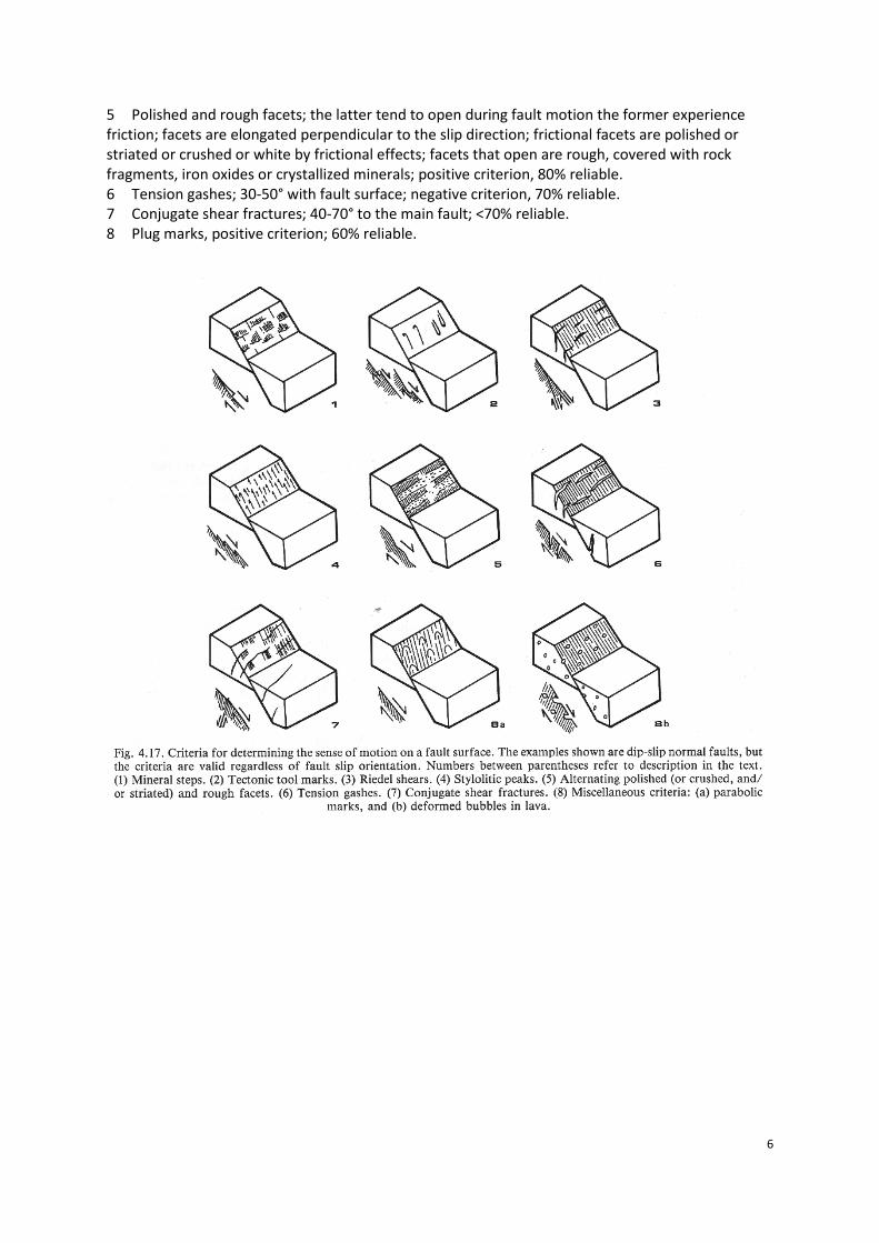
5 Polished and rough facets; the latter tend to open during fault motion the former experience friction; facets are elongated perpendicular to the slip direction; frictional facets are polished or striated or crushed or white by frictional effects; facets that open are rough, covered with rock fragments, iron oxides or crystallized minerals; positive criterion, 80% reliable. 6 Tension gashes; 30-50° with fault surface; negative criterion, 70% reliable. 7 Conjugate shear fractures; 40-70° to the main fault; <70% reliable. 8 Plug marks, positive criterion; 60% reliable.

7

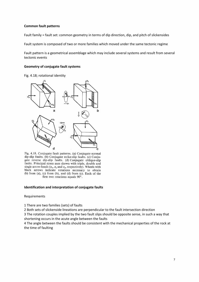
Common fault patterns Fault family = fault set: common geometry in terms of dip direction, dip, and pitch of slickensides Fault system is composed of two or more families which moved under the same tectonic regime Fault pattern is a geometrical assemblage which may include several systems and result from several tectonic events Geometry of conjugate fault systems Fig. 4.18; rotational identity

Identification and interpretation of conjugate faults Requirements 1 There are two families (sets) of faults 2 Both sets of slickenside lineations are perpendicular to the fault intersection direction 3 The rotation couples implied by the two fault slips should be opposite sense, in such a way that shortening occurs in the acute angle between the faults 4 The angle between the faults should be consistent with the mechanical properties of the rock at the time of faulting

8

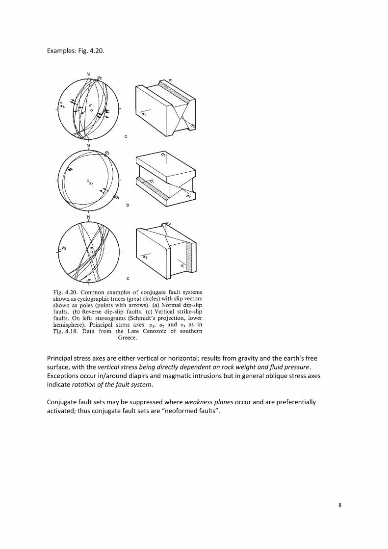
Examples: Fig. 4.20.

Principal stress axes are either vertical or horizontal; results from gravity and the earth’s free surface, with the vertical stress being directly dependent on rock weight and fluid pressure. Exceptions occur in/around diapirs and magmatic intrusions but in general oblique stress axes indicate rotation of the fault system. Conjugate fault sets may be suppressed where weakness planes occur and are preferentially activated; thus conjugate fault sets are “neoformed faults”.

9

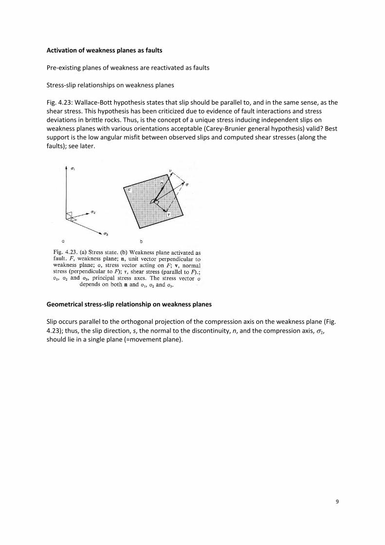
Activation of weakness planes as faults Pre-existing planes of weakness are reactivated as faults Stress-slip relationships on weakness planes Fig. 4.23: Wallace-Bott hypothesis states that slip should be parallel to, and in the same sense, as the shear stress. This hypothesis has been criticized due to evidence of fault interactions and stress deviations in brittle rocks. Thus, is the concept of a unique stress inducing independent slips on weakness planes with various orientations acceptable (Carey-Brunier general hypothesis) valid? Best support is the low angular misfit between observed slips and computed shear stresses (along the faults); see later.

Geometrical stress-slip relationship on weakness planes Slip occurs parallel to the orthogonal projection of the compression axis on the weakness plane (Fig.

4.23); thus, the slip direction, s, the normal to the discontinuity, n, and the compression axis, 1, should lie in a single plane (=movement plane).

10

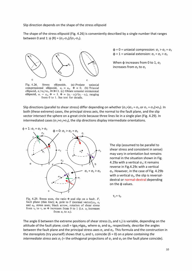
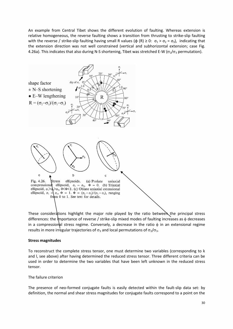
Slip direction depends on the shape of the stress ellipsoid The shape of the stress ellipsoid (Fig. 4.26) is conveniently described by a single number that ranges

between 0 and 1: (R) = (2-3)/(1-3).

Slip directions (parallel to shear stress) differ depending on whether (1>)2 = 3 or 1 = 2(>3). In both (these extreme) cases, the principal stress axis, the normal to the fault plane, and the slip vector intersect the sphere on a great circle because three lines lie in a single plan (Fig. 4.29). In

intermediated cases (1>2>3), the slip directions display intermediate orientations.

The angle δ between the extreme positions of shear stress (τ0 and τ1) is variable, depending on the attitude of the fault plane; cosδ = tgα1×tgα3, where α1 and α3, respectively, describe the angles between the fault plane and the principal stress axes σ1 and σ3. This formula and the construction in the stereoplots (try yourself) shows that τ0 and τ1 coincide (δ = 0) on a plane containing the intermediate stress axis σ2 (= the orthogonal projections of σ1 and σ3 on the fault plane coincide).

φ = 0 = uniaxial compression: σ1 > σ2 = σ3 φ = 1 = uniaxial extension: σ1 = σ2 > σ3

When φ increases from 0 to 1, σ2 increases from σ3 to σ1

The slip (assumed to be parallel to shear stress and consistent in sense) may vary in orientation but remains normal in the situation shown in Fig. 4.29a with a vertical σ1; it remains reverse in Fig.4.29c with a vertical σ3. However, in the case of Fig. 4.29b with a vertical σ2, the slip is reversal-dextral or normal-dextral depending on the φ values.

φ = 0: σ1 > σ2 = σ3

= 1: σ1 = σ2 > σ3

σ1 = σ2 > σ3

τ2 = τ0

11

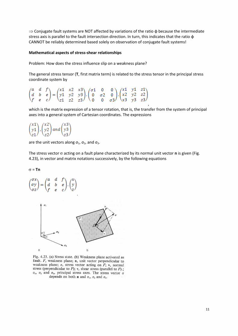
Conjugate fault systems are NOT affected by variations of the ratio φ because the intermediate stress axis is parallel to the fault intersection direction. In turn, this indicates that the ratio φ CANNOT be reliably determined based solely on observation of conjugate fault systems! Mathematical aspects of stress-shear relationships Problem: How does the stress influence slip on a weakness plane? The general stress tensor (T, first matrix term) is related to the stress tensor in the principal stress coordinate system by

, which is the matrix expression of a tensor rotation, that is, the transfer from the system of principal axes into a general system of Cartesian coordinates. The expressions

are the unit vectors along σ1, σ2, and σ3.

The stress vector acting on a fault plane characterized by its normal unit vector n is given (Fig. 4.23), in vector and matrix notations successively, by the following equations

= Tn

.

12

The modulus (Betrag) of the normal stress ν is given by the scalar product of the stress vector by the unit normal vector

oder .

The normal stress vector, ν, is then

or

.

Knowing the stress vector σ and the normal stress vector ν, the shear stress vector τ is

σ = ν + τ that is

.

Reduced stress tensor: by adding to the stress tensor an isotropic stress defined by l = –σ3, then multiplying the tensor by the positive constant k = 1/(σ1-σ3), one obtains

→ , both tensors are equivalent in terms of directions and senses of

shear stresses (remember = (2-3)/(1-3)). The resulting “reduced stress tensor” contains four independent variables, and simply depends on the orientation of the principal stress axes and the ratio φ

.

The variables k and l (see above) cannot be determined from fault-slip orientations and senses. As the reduced stress tensor has four independent variables, one needs four distinct fault-slip data are necessary to calculate it!

13

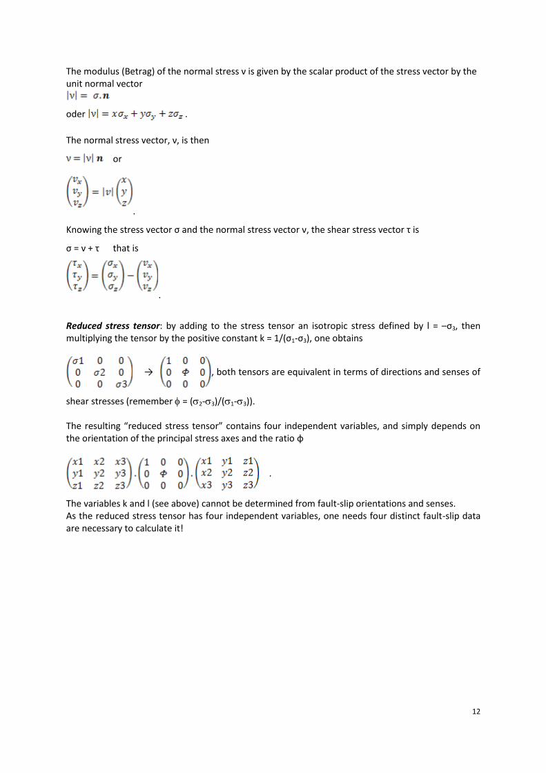
How does a single fault constrain paleostress? An extensional tectonic regime (σ1 vertical) induces fault slips with normal components of motion, whereas a compressional regime induces reverse components (Fig. 4.31 a, b). For a vertical σ2 axis, the sense of the lateral component of motion also depends on the strike of the fault, but the sense of the transverse component, reverse or normal, is variable as a function of the angle between the strike and, say, the σ3 axis. The threshold angle, β, between the normal and reverse components depends on the ratio φ (Fig, 4.31c; tg2β = (1-φ)/φ).

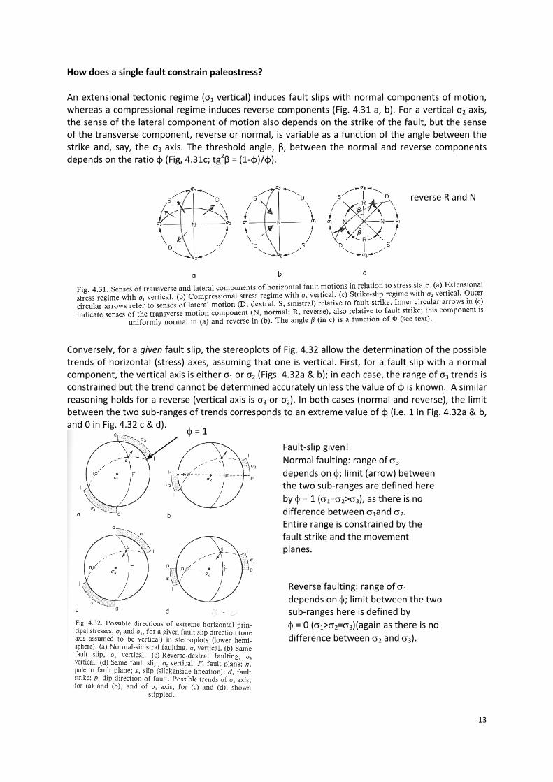
Conversely, for a given fault slip, the stereoplots of Fig. 4.32 allow the determination of the possible trends of horizontal (stress) axes, assuming that one is vertical. First, for a fault slip with a normal component, the vertical axis is either σ1 or σ2 (Figs. 4.32a & b); in each case, the range of σ3 trends is constrained but the trend cannot be determined accurately unless the value of φ is known. A similar reasoning holds for a reverse (vertical axis is σ3 or σ2). In both cases (normal and reverse), the limit between the two sub-ranges of trends corresponds to an extreme value of φ (i.e. 1 in Fig. 4.32a & b, and 0 in Fig. 4.32 c & d).

reverse R and N

Fault-slip given!

Normal faulting: range of 3

depends on ; limit (arrow) between the two sub-ranges are defined here

by = 1 (1=2>3), as there is no

difference between 1and 2. Entire range is constrained by the fault strike and the movement planes.

Reverse faulting: range of 1

depends on ; limit between the two sub-ranges here is defined by

= 0 (1>2=3)(again as there is no

difference between 2 and 3).

= 1

14

The right dihedra (or P and T method) and the focal mechanism of a fault

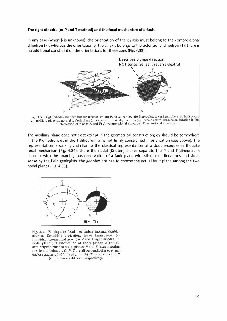
In any case (when is unknown), the orientation of the 1 axis must belong to the compressional

dihedron (P), whereas the orientation of the 3 axis belongs to the extensional dihedron (T); there is no additional constraint on the orientations for these axes (Fig. 4.33).

The auxiliary plane does not exist except in the geometrical construction; 1 should be somewhere

in the P dihedron, 3 in the T dihedron; 2 is not firmly constrained in orientation (see above). The representation is strikingly similar to the classical representation of a double-couple earthquake focal mechanism (Fig. 4.34); there the nodal (Knoten) planes separate the P and T dihedral. In contrast with the unambiguous observation of a fault plane with slickenside lineations and shear sense by the field geologists, the geophysicist has to choose the actual fault plane among the two nodal planes (Fig. 4.35).

Describes plunge direction NOT sense! Sense is reverse-dextral

15

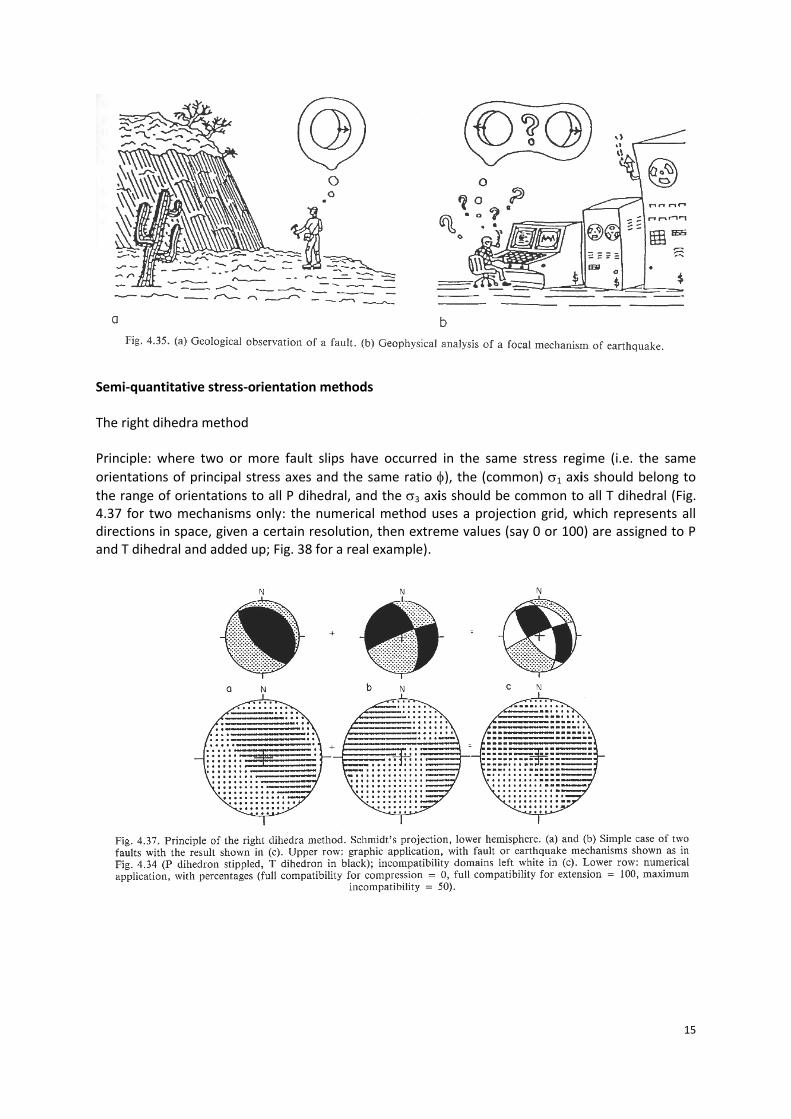
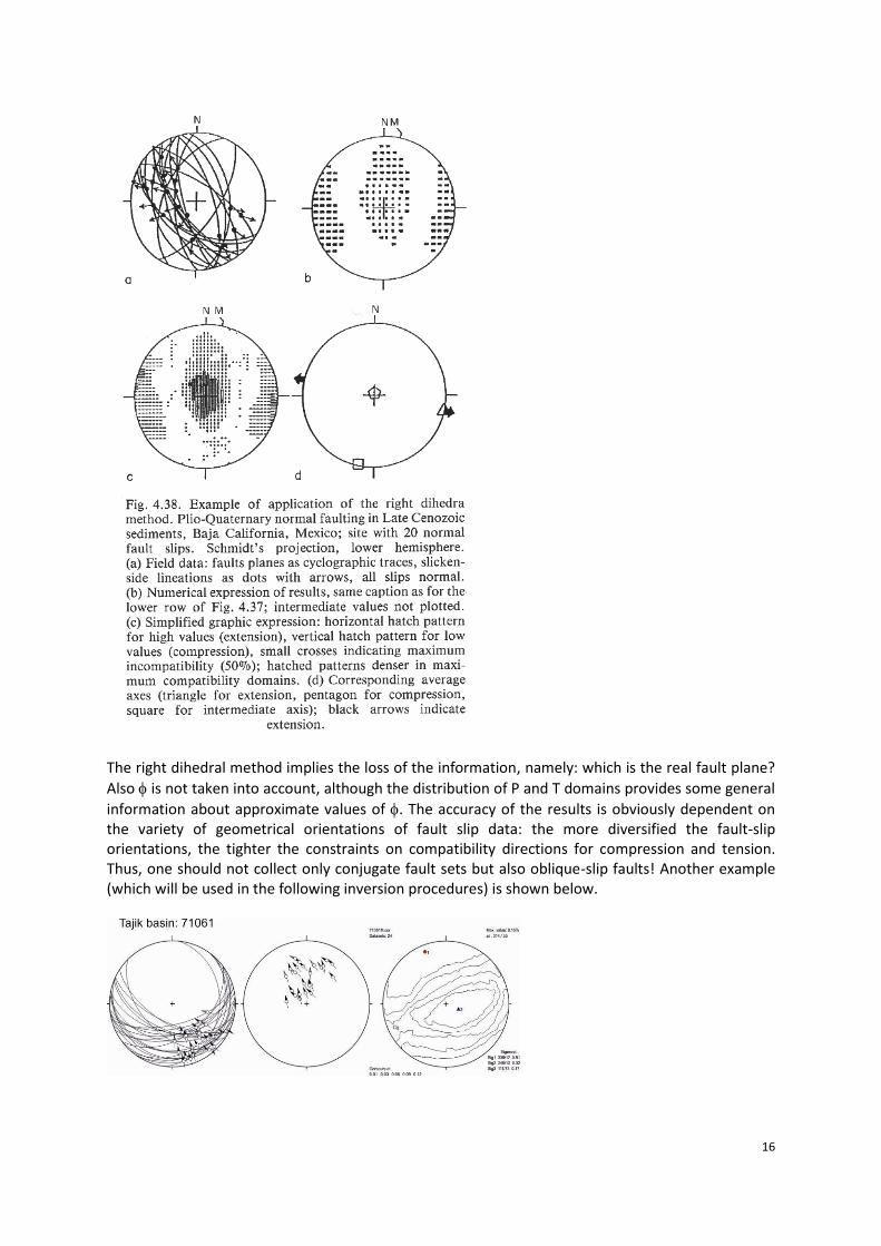
Semi-quantitative stress-orientation methods The right dihedra method Principle: where two or more fault slips have occurred in the same stress regime (i.e. the same

orientations of principal stress axes and the same ratio ), the (common) 1 axis should belong to

the range of orientations to all P dihedral, and the 3 axis should be common to all T dihedral (Fig. 4.37 for two mechanisms only: the numerical method uses a projection grid, which represents all directions in space, given a certain resolution, then extreme values (say 0 or 100) are assigned to P and T dihedral and added up; Fig. 38 for a real example).

16

The right dihedral method implies the loss of the information, namely: which is the real fault plane?

Also is not taken into account, although the distribution of P and T domains provides some general

information about approximate values of . The accuracy of the results is obviously dependent on the variety of geometrical orientations of fault slip data: the more diversified the fault-slip orientations, the tighter the constraints on compatibility directions for compression and tension. Thus, one should not collect only conjugate fault sets but also oblique-slip faults! Another example (which will be used in the following inversion procedures) is shown below.

17

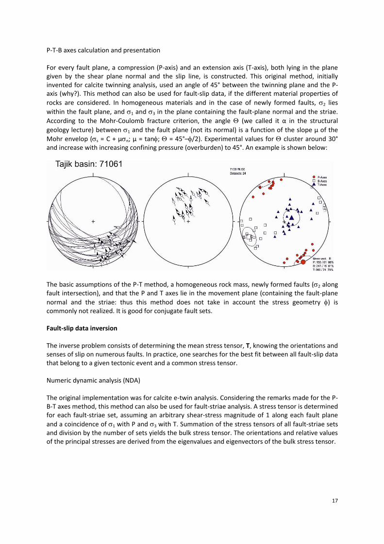
P-T-B axes calculation and presentation For every fault plane, a compression (P-axis) and an extension axis (T-axis), both lying in the plane given by the shear plane normal and the slip line, is constructed. This original method, initially invented for calcite twinning analysis, used an angle of 45° between the twinning plane and the P-axis (why?). This method can also be used for fault-slip data, if the different material properties of

rocks are considered. In homogeneous materials and in the case of newly formed faults, 2 lies

within the fault plane, and 1 and 3 in the plane containing the fault-plane normal and the striae.

According to the Mohr-Coulomb fracture criterion, the angle (we called it α in the structural

geology lecture) between 1 and the fault plane (not its normal) is a function of the slope μ of the

Mohr envelop (s = C + μn; μ = tan; = 45°–/2). Experimental values for cluster around 30° and increase with increasing confining pressure (overburden) to 45°. An example is shown below:

The basic assumptions of the P-T method, a homogeneous rock mass, newly formed faults (2 along fault intersection), and that the P and T axes lie in the movement plane (containing the fault-plane

normal and the striae: thus this method does not take in account the stress geometry ) is commonly not realized. It is good for conjugate fault sets. Fault-slip data inversion The inverse problem consists of determining the mean stress tensor, T, knowing the orientations and senses of slip on numerous faults. In practice, one searches for the best fit between all fault-slip data that belong to a given tectonic event and a common stress tensor. Numeric dynamic analysis (NDA) The original implementation was for calcite e-twin analysis. Considering the remarks made for the P-B-T axes method, this method can also be used for fault-striae analysis. A stress tensor is determined for each fault-striae set, assuming an arbitrary shear-stress magnitude of 1 along each fault plane

and a coincidence of 1 with P and 3 with T. Summation of the stress tensors of all fault-striae sets and division by the number of sets yields the bulk stress tensor. The orientations and relative values of the principal stresses are derived from the eigenvalues and eigenvectors of the bulk stress tensor.

18

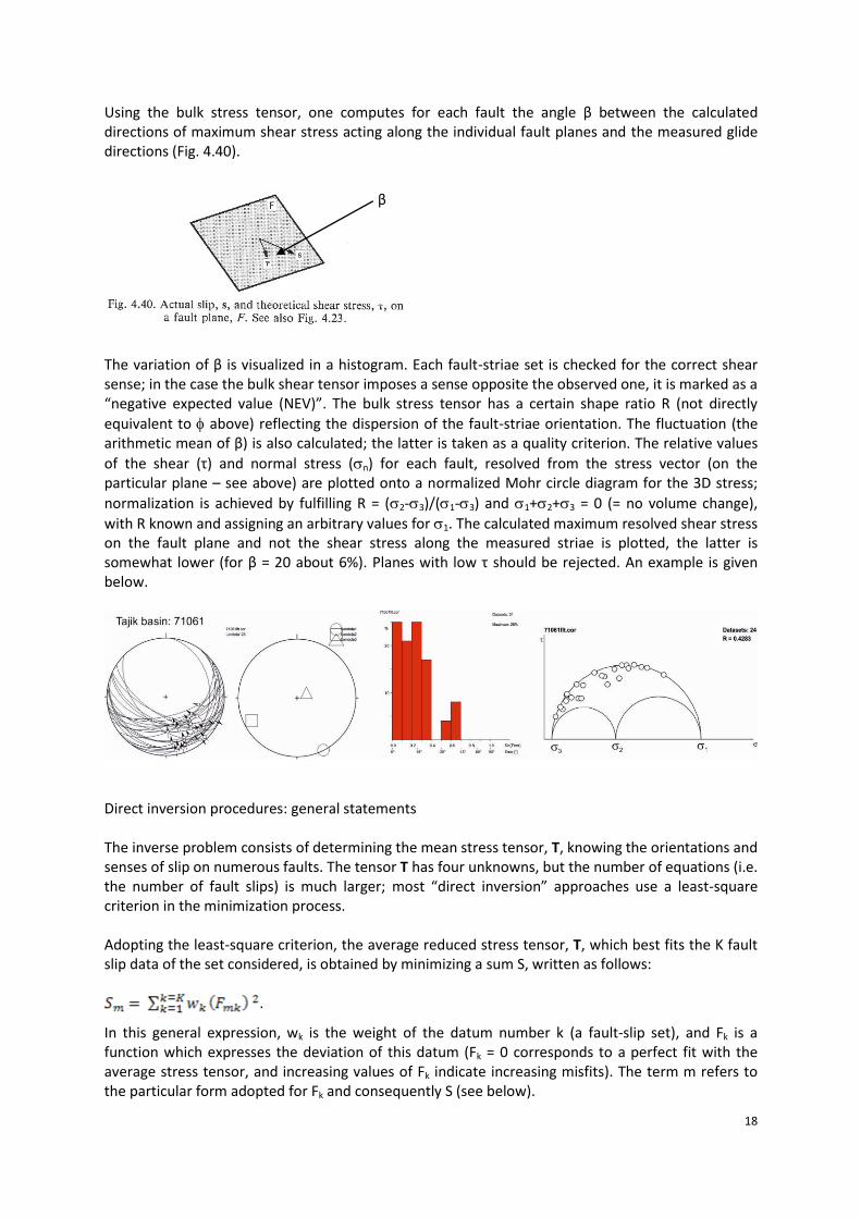
Using the bulk stress tensor, one computes for each fault the angle β between the calculated directions of maximum shear stress acting along the individual fault planes and the measured glide directions (Fig. 4.40).

The variation of β is visualized in a histogram. Each fault-striae set is checked for the correct shear sense; in the case the bulk shear tensor imposes a sense opposite the observed one, it is marked as a “negative expected value (NEV)”. The bulk stress tensor has a certain shape ratio R (not directly

equivalent to above) reflecting the dispersion of the fault-striae orientation. The fluctuation (the arithmetic mean of β) is also calculated; the latter is taken as a quality criterion. The relative values

of the shear (τ) and normal stress (n) for each fault, resolved from the stress vector (on the particular plane – see above) are plotted onto a normalized Mohr circle diagram for the 3D stress;

normalization is achieved by fulfilling R = (2-3)/(1-3) and 1+2+3 = 0 (= no volume change),

with R known and assigning an arbitrary values for 1. The calculated maximum resolved shear stress on the fault plane and not the shear stress along the measured striae is plotted, the latter is somewhat lower (for β = 20 about 6%). Planes with low τ should be rejected. An example is given below.

Direct inversion procedures: general statements The inverse problem consists of determining the mean stress tensor, T, knowing the orientations and senses of slip on numerous faults. The tensor T has four unknowns, but the number of equations (i.e. the number of fault slips) is much larger; most “direct inversion” approaches use a least-square criterion in the minimization process. Adopting the least-square criterion, the average reduced stress tensor, T, which best fits the K fault slip data of the set considered, is obtained by minimizing a sum S, written as follows:

.

In this general expression, wk is the weight of the datum number k (a fault-slip set), and Fk is a function which expresses the deviation of this datum (Fk = 0 corresponds to a perfect fit with the average stress tensor, and increasing values of Fk indicate increasing misfits). The term m refers to the particular form adopted for Fk and consequently S (see below).

β

19

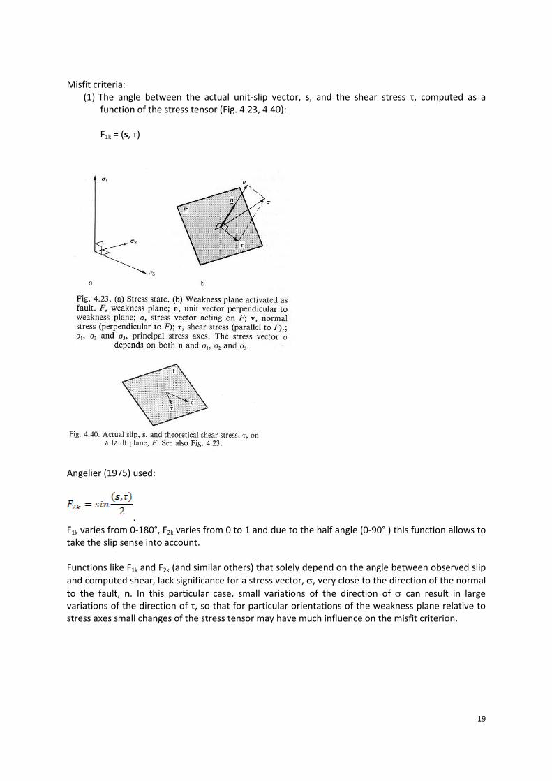
Misfit criteria:

(1) The angle between the actual unit-slip vector, s, and the shear stress τ, computed as a function of the stress tensor (Fig. 4.23, 4.40): F1k = (s, τ)

Angelier (1975) used:

. F1k varies from 0-180°, F2k varies from 0 to 1 and due to the half angle (0-90° ) this function allows to take the slip sense into account. Functions like F1k and F2k (and similar others) that solely depend on the angle between observed slip

and computed shear, lack significance for a stress vector, , very close to the direction of the normal

to the fault, n. In this particular case, small variations of the direction of can result in large variations of the direction of τ, so that for particular orientations of the weakness plane relative to stress axes small changes of the stress tensor may have much influence on the misfit criterion.

20

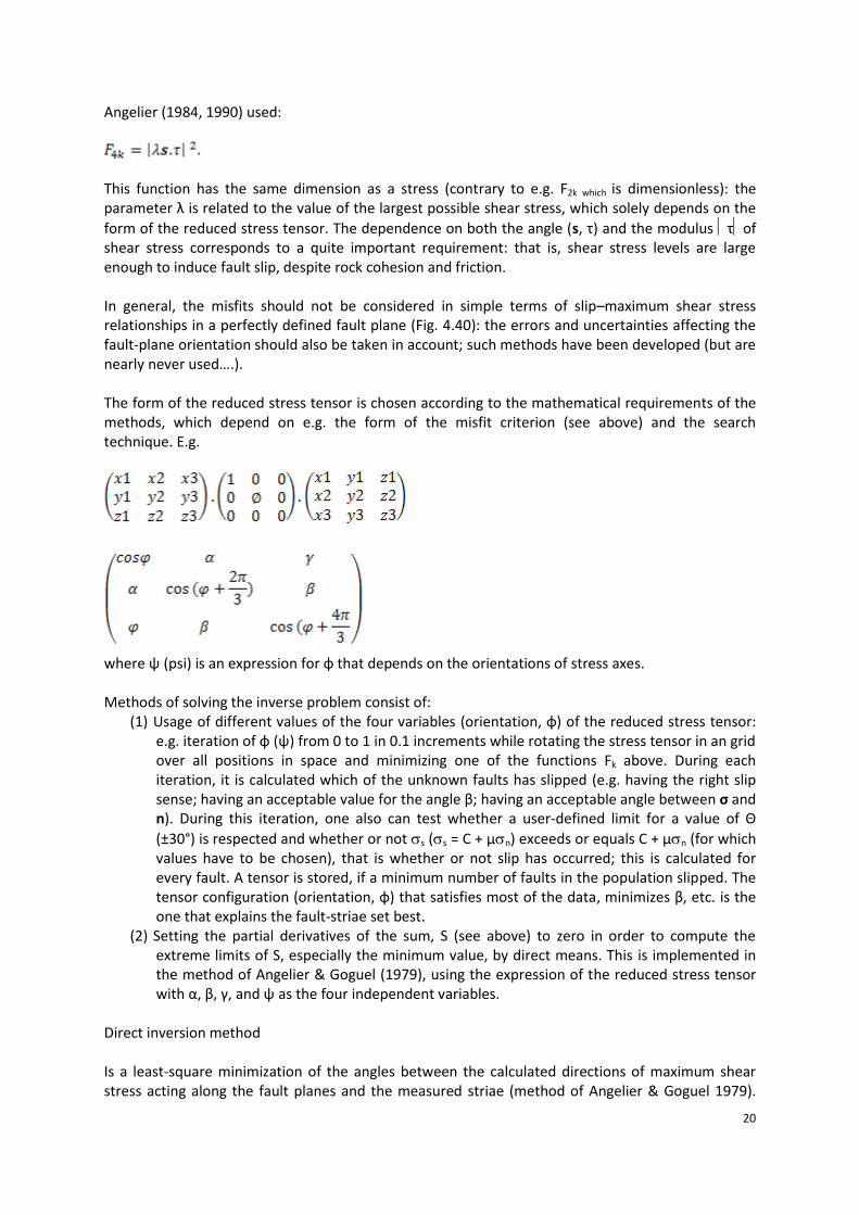
Angelier (1984, 1990) used:

This function has the same dimension as a stress (contrary to e.g. F2k which is dimensionless): the parameter λ is related to the value of the largest possible shear stress, which solely depends on the

form of the reduced stress tensor. The dependence on both the angle (s, τ) and the modulus τof shear stress corresponds to a quite important requirement: that is, shear stress levels are large enough to induce fault slip, despite rock cohesion and friction. In general, the misfits should not be considered in simple terms of slip–maximum shear stress relationships in a perfectly defined fault plane (Fig. 4.40): the errors and uncertainties affecting the fault-plane orientation should also be taken in account; such methods have been developed (but are nearly never used….). The form of the reduced stress tensor is chosen according to the mathematical requirements of the methods, which depend on e.g. the form of the misfit criterion (see above) and the search technique. E.g.

where ψ (psi) is an expression for φ that depends on the orientations of stress axes. Methods of solving the inverse problem consist of:

(1) Usage of different values of the four variables (orientation, φ) of the reduced stress tensor: e.g. iteration of φ (ψ) from 0 to 1 in 0.1 increments while rotating the stress tensor in an grid over all positions in space and minimizing one of the functions Fk above. During each iteration, it is calculated which of the unknown faults has slipped (e.g. having the right slip sense; having an acceptable value for the angle β; having an acceptable angle between σ and n). During this iteration, one also can test whether a user-defined limit for a value of Θ

(±30°) is respected and whether or not s (s = C + μn) exceeds or equals C + μn (for which values have to be chosen), that is whether or not slip has occurred; this is calculated for every fault. A tensor is stored, if a minimum number of faults in the population slipped. The tensor configuration (orientation, φ) that satisfies most of the data, minimizes β, etc. is the one that explains the fault-striae set best.

(2) Setting the partial derivatives of the sum, S (see above) to zero in order to compute the extreme limits of S, especially the minimum value, by direct means. This is implemented in the method of Angelier & Goguel (1979), using the expression of the reduced stress tensor with α, β, γ, and ψ as the four independent variables.

Direct inversion method Is a least-square minimization of the angles between the calculated directions of maximum shear stress acting along the fault planes and the measured striae (method of Angelier & Goguel 1979).

21

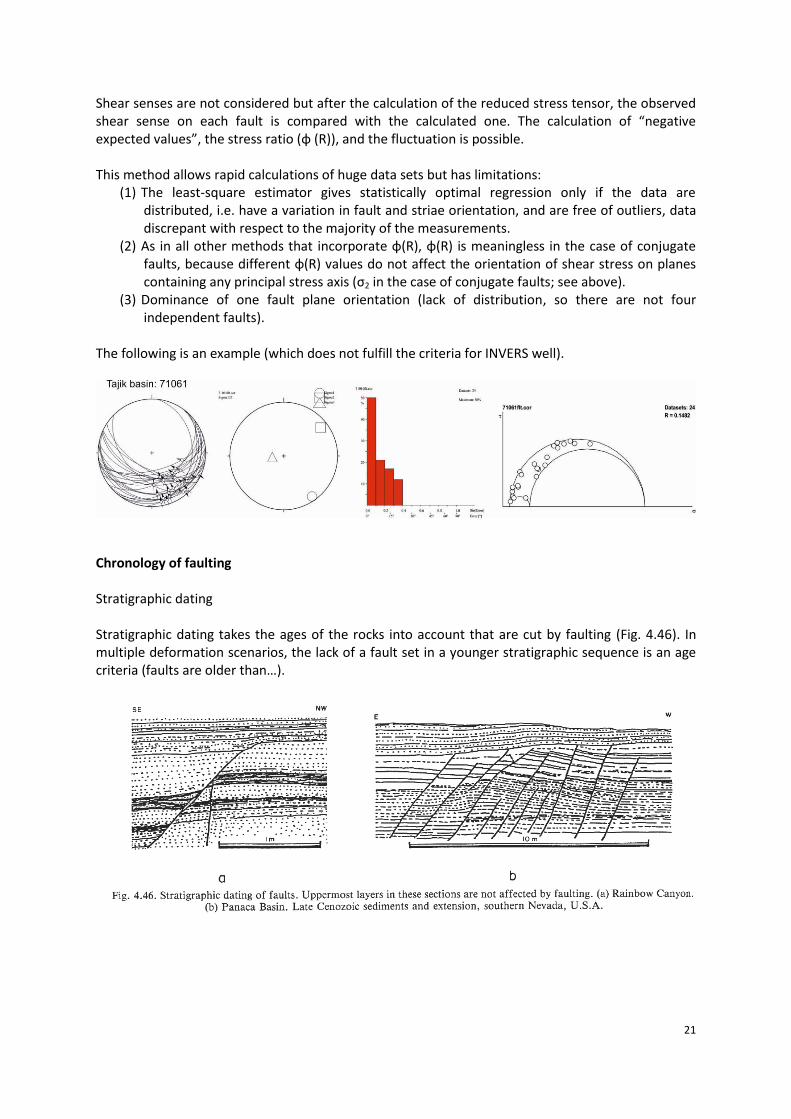
Shear senses are not considered but after the calculation of the reduced stress tensor, the observed shear sense on each fault is compared with the calculated one. The calculation of “negative expected values”, the stress ratio (φ (R)), and the fluctuation is possible. This method allows rapid calculations of huge data sets but has limitations:

(1) The least-square estimator gives statistically optimal regression only if the data are distributed, i.e. have a variation in fault and striae orientation, and are free of outliers, data discrepant with respect to the majority of the measurements.

(2) As in all other methods that incorporate φ(R), φ(R) is meaningless in the case of conjugate faults, because different φ(R) values do not affect the orientation of shear stress on planes containing any principal stress axis (σ2 in the case of conjugate faults; see above).

(3) Dominance of one fault plane orientation (lack of distribution, so there are not four independent faults).

The following is an example (which does not fulfill the criteria for INVERS well).

Chronology of faulting Stratigraphic dating Stratigraphic dating takes the ages of the rocks into account that are cut by faulting (Fig. 4.46). In multiple deformation scenarios, the lack of a fault set in a younger stratigraphic sequence is an age criteria (faults are older than…).

22

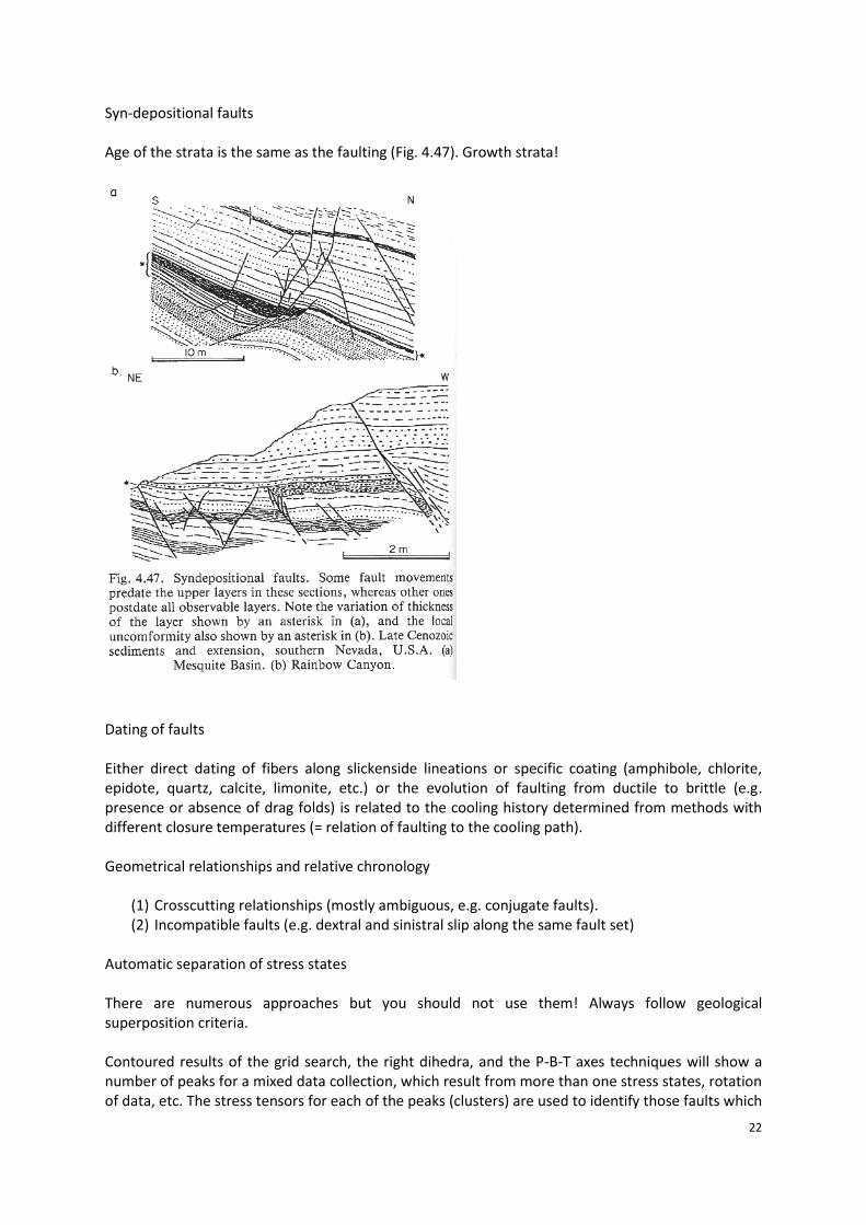
Syn-depositional faults Age of the strata is the same as the faulting (Fig. 4.47). Growth strata!

Dating of faults Either direct dating of fibers along slickenside lineations or specific coating (amphibole, chlorite, epidote, quartz, calcite, limonite, etc.) or the evolution of faulting from ductile to brittle (e.g. presence or absence of drag folds) is related to the cooling history determined from methods with different closure temperatures (= relation of faulting to the cooling path). Geometrical relationships and relative chronology

(1) Crosscutting relationships (mostly ambiguous, e.g. conjugate faults). (2) Incompatible faults (e.g. dextral and sinistral slip along the same fault set)

Automatic separation of stress states There are numerous approaches but you should not use them! Always follow geological superposition criteria. Contoured results of the grid search, the right dihedra, and the P-B-T axes techniques will show a number of peaks for a mixed data collection, which result from more than one stress states, rotation of data, etc. The stress tensors for each of the peaks (clusters) are used to identify those faults which

23

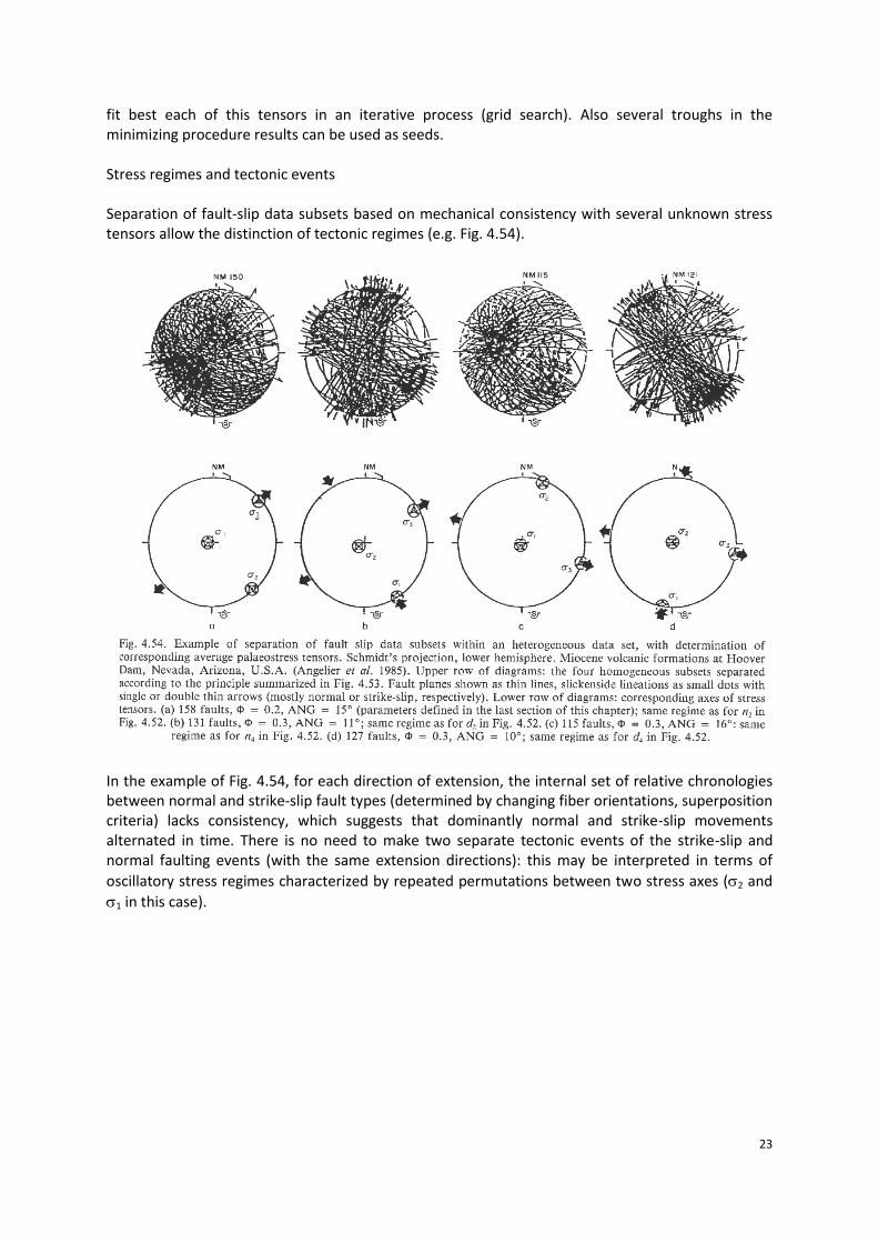
fit best each of this tensors in an iterative process (grid search). Also several troughs in the minimizing procedure results can be used as seeds. Stress regimes and tectonic events Separation of fault-slip data subsets based on mechanical consistency with several unknown stress tensors allow the distinction of tectonic regimes (e.g. Fig. 4.54).

In the example of Fig. 4.54, for each direction of extension, the internal set of relative chronologies between normal and strike-slip fault types (determined by changing fiber orientations, superposition criteria) lacks consistency, which suggests that dominantly normal and strike-slip movements alternated in time. There is no need to make two separate tectonic events of the strike-slip and normal faulting events (with the same extension directions): this may be interpreted in terms of

oscillatory stress regimes characterized by repeated permutations between two stress axes (2 and

1 in this case).

24

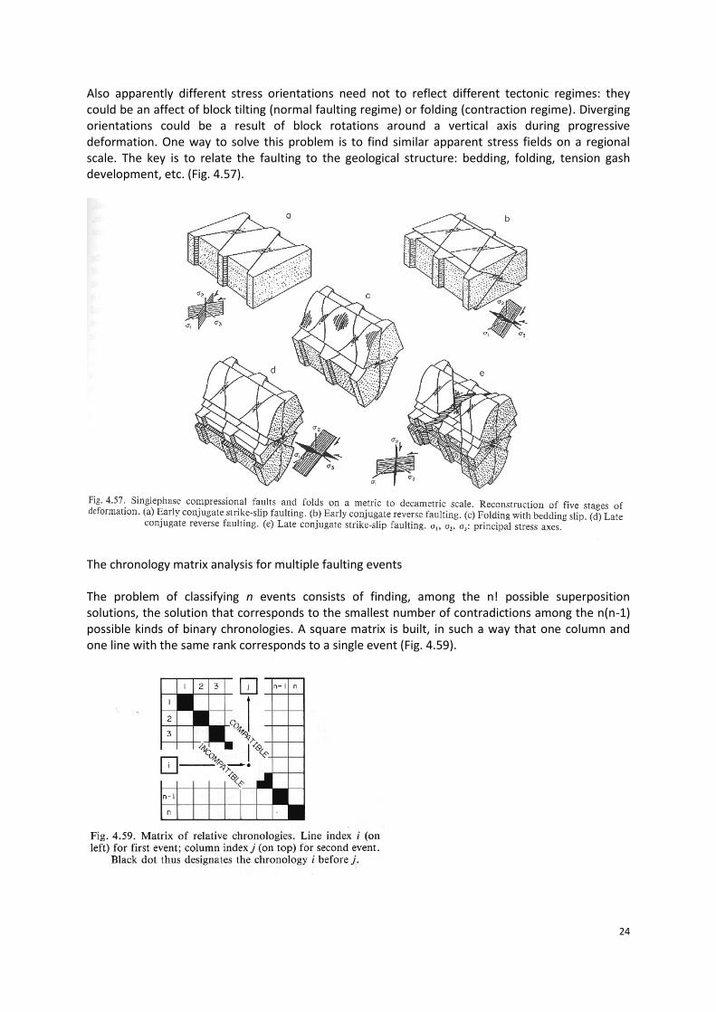
Also apparently different stress orientations need not to reflect different tectonic regimes: they could be an affect of block tilting (normal faulting regime) or folding (contraction regime). Diverging orientations could be a result of block rotations around a vertical axis during progressive deformation. One way to solve this problem is to find similar apparent stress fields on a regional scale. The key is to relate the faulting to the geological structure: bedding, folding, tension gash development, etc. (Fig. 4.57).

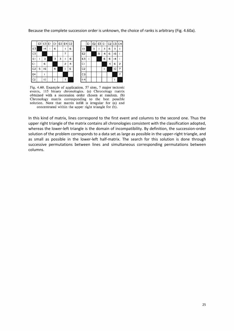
The chronology matrix analysis for multiple faulting events The problem of classifying n events consists of finding, among the n! possible superposition solutions, the solution that corresponds to the smallest number of contradictions among the n(n-1) possible kinds of binary chronologies. A square matrix is built, in such a way that one column and one line with the same rank corresponds to a single event (Fig. 4.59).

25

Because the complete succession order is unknown, the choice of ranks is arbitrary (Fig. 4.60a).

In this kind of matrix, lines correspond to the first event and columns to the second one. Thus the upper right triangle of the matrix contains all chronologies consistent with the classification adopted, whereas the lower-left triangle is the domain of incompatibility. By definition, the succession-order solution of the problem corresponds to a data set as large as possible in the upper-right triangle, and as small as possible in the lower-left half-matrix. The search for this solution is done through successive permutations between lines and simultaneous corresponding permutations between columns.

26

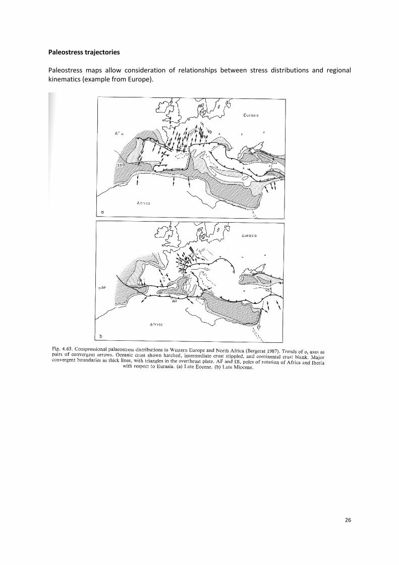
Paleostress trajectories Paleostress maps allow consideration of relationships between stress distributions and regional kinematics (example from Europe).

27

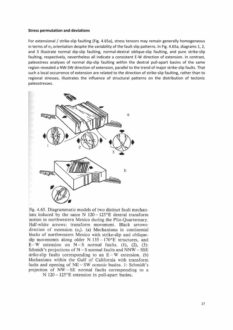
Stress permutation and deviations For extensional / strike-slip faulting (Fig. 4.65a), stress tensors may remain generally homogeneous

in terms of 3 orientation despite the variability of the fault-slip patterns. In Fig. 4.65a, diagrams 1, 2, and 3 illustrate normal dip-slip faulting, normal-dextral oblique-slip faulting, and pure strike-slip faulting, respectively, nevertheless all indicate a consistent E-W direction of extension. In contrast, paleostress analyses of normal dip-slip faulting within the dextral pull-apart basins of the same region revealed a NW-SW direction of extension, parallel to the trend of major strike-slip faults. That such a local occurrence of extension are related to the direction of strike-slip faulting, rather than to regional stresses, illustrates the influence of structural patterns on the distribution of tectonic paleostresses.

28

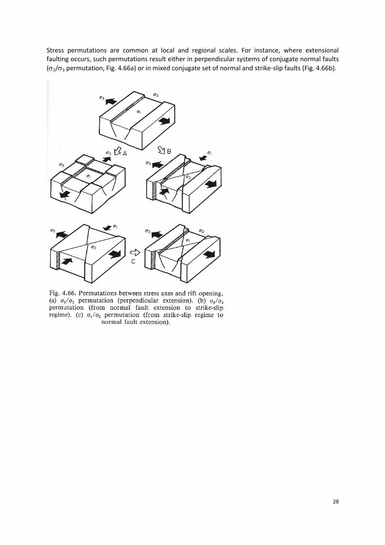
Stress permutations are common at local and regional scales. For instance, where extensional faulting occurs, such permutations result either in perpendicular systems of conjugate normal faults

(2/3 permutation, Fig. 4.66a) or in mixed conjugate set of normal and strike-slip faults (Fig. 4.66b).

29

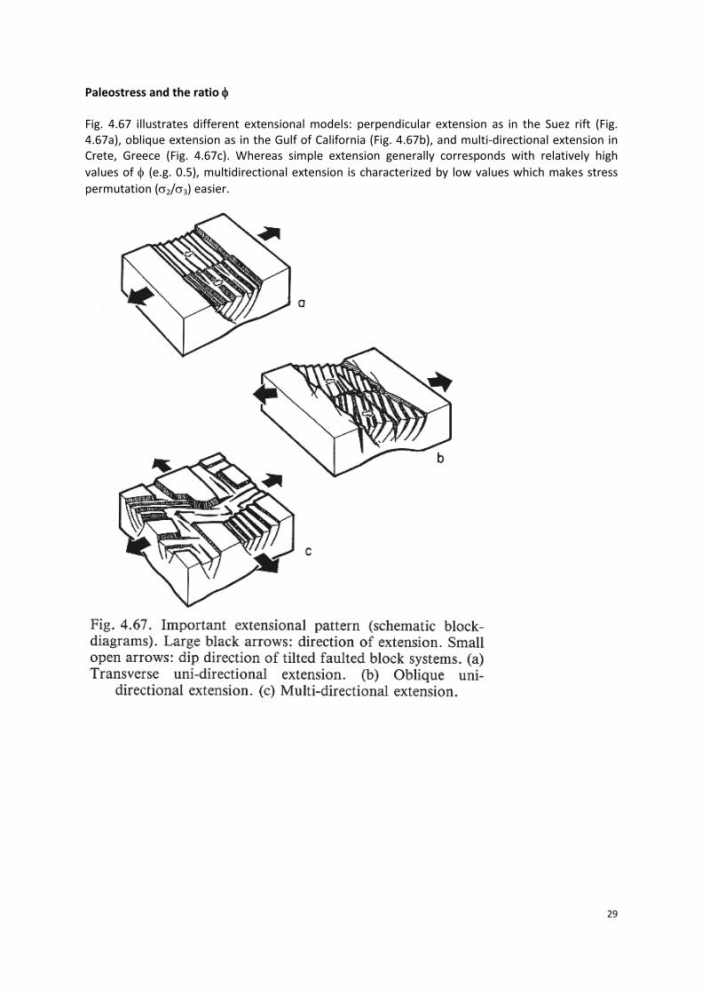
Paleostress and the ratio Fig. 4.67 illustrates different extensional models: perpendicular extension as in the Suez rift (Fig. 4.67a), oblique extension as in the Gulf of California (Fig. 4.67b), and multi-directional extension in Crete, Greece (Fig. 4.67c). Whereas simple extension generally corresponds with relatively high

values of (e.g. 0.5), multidirectional extension is characterized by low values which makes stress

permutation (2/3) easier.

30

An example from Central Tibet shows the different evolution of faulting. Whereas extension is relative homogeneous, the reverse faulting shows a transition from thrusting to strike-slip faulting with the reverse / strike-slip faulting having small R values (φ (R) ≥ 0: σ1 > σ2 = σ3), indicating that the extension direction was not well constrained (vertical and subhorizontal extension; case Fig.

4.26a). This indicates that also during N-S shortening, Tibet was stretched E-W (2/3 permutation).

These considerations highlight the major role played by the ratio between the principal stress

differences: the importance of reverse / strike-slip mixed modes of faulting increases as decreases

in a compressional stress regime. Conversely, a decrease in the ratio in an extensional regime

results in more irregular trajectories of 3 and local permutations of 2/3. Stress magnitudes To reconstruct the complete stress tensor, one must determine two variables (corresponding to k and l, see above) after having determined the reduced stress tensor. Three different criteria can be used in order to determine the two variables that have been left unknown in the reduced stress tensor. The failure criterion The presence of neo-formed conjugate faults is easily detected within the fault-slip data set: by definition, the normal and shear stress magnitudes for conjugate faults correspond to a point on the

31

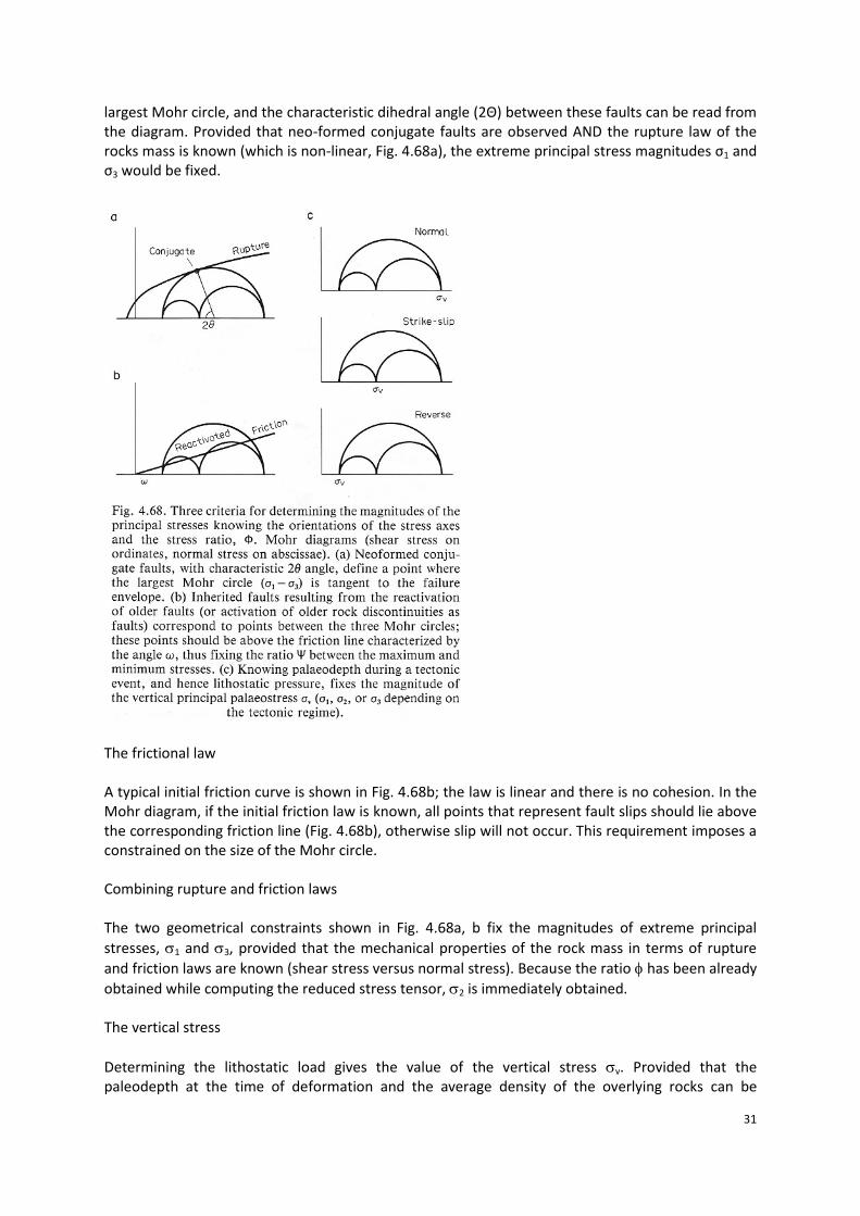
largest Mohr circle, and the characteristic dihedral angle (2Θ) between these faults can be read from the diagram. Provided that neo-formed conjugate faults are observed AND the rupture law of the rocks mass is known (which is non-linear, Fig. 4.68a), the extreme principal stress magnitudes σ1 and σ3 would be fixed.

The frictional law A typical initial friction curve is shown in Fig. 4.68b; the law is linear and there is no cohesion. In the Mohr diagram, if the initial friction law is known, all points that represent fault slips should lie above the corresponding friction line (Fig. 4.68b), otherwise slip will not occur. This requirement imposes a constrained on the size of the Mohr circle. Combining rupture and friction laws The two geometrical constraints shown in Fig. 4.68a, b fix the magnitudes of extreme principal

stresses, 1 and 3, provided that the mechanical properties of the rock mass in terms of rupture

and friction laws are known (shear stress versus normal stress). Because the ratio has been already

obtained while computing the reduced stress tensor, 2 is immediately obtained. The vertical stress

Determining the lithostatic load gives the value of the vertical stress v. Provided that the paleodepth at the time of deformation and the average density of the overlying rocks can be

32

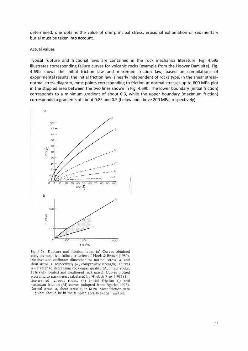
determined, one obtains the value of one principal stress; erosional exhumation or sedimentary burial must be taken into account. Actual values Typical rupture and frictional laws are contained in the rock mechanics literature. Fig. 4.69a illustrates corresponding failure curves for volcanic rocks (example from the Hoover Dam site). Fig. 4.69b shows the initial friction law and maximum friction law, based on compilations of experimental results; the initial friction law is nearly independent of rocks type. In the shear stress–normal stress diagram, most points corresponding to friction at normal stresses up to 600 MPa plot in the stippled area between the two lines shown in Fig. 4.69b. The lower boundary (initial friction) corresponds to a minimum gradient of about 0.3, while the upper boundary (maximum friction) corresponds to gradients of about 0.85 and 0.5 (below and above 200 MPa, respectively).

33

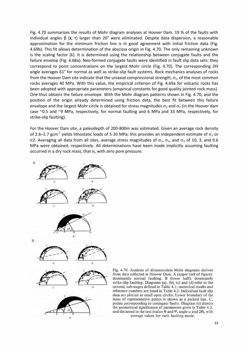
Fig. 4.70 summarizes the results of Mohr diagram analyses at Hoover Dam. 19 % of the faults with individual angles β (s, τ) larger than 20° were eliminated. Despite data dispersion, a reasonable approximation for the minimum friction line is in good agreement with initial friction data (Fig. 4.69b). This fit allows determination of the abscissa origin in Fig. 4.70. The only remaining unknown is the scaling factor (k). It is determined using the relationship between conjugate faults and the failure envelop (Fig. 4.68a). Neo-formed conjugate faults were identified in fault slip data sets: they

correspond to point concentrations on the largest Mohr circle (Fig. 4.70). The corresponding 2 angle averages 61° for normal as well as strike-slip fault systems. Rock mechanics analyses of rocks

from the Hoover Dam site indicate that the uniaxial compressional strength, c, of the most common rocks averages 40 MPa. With this value, the empirical criterion of Fig. 4.69a for volcanic rocks has been adopted with appropriate parameters (empirical constants for good quality jointed rock mass). One thus obtains the failure envelope. With the Mohr diagram patterns shown in Fig. 4.70, and the position of the origin already determined using friction data, the best fit between this failure

envelope and the largest Mohr circle is obtained for stress magnitudes 3 and 1 (in the Hoover dam case ~0.5 and ~9 MPa, respectively, for normal faulting and 6 MPa and 33 MPa, respectively, for strike-slip faulting). For the Hoover Dam site, a paleodepth of 200-800m was estimated. Given an average rock density

of 2.6–2.7 gcm-2 yields lithostatic loads of 5-20 MPa; this provides an independent estimate of 1 or

2. Averaging all data from all sites, average stress magnitudes of 1, 2, and 3 of 10, 3, and 0.6 MPa were obtained, respectively. All determinations have been made implicitly assuming faulting occurred in a dry rock mass, that is, with zero pore pressure.