Factorized scattering in the presence of reflecting boundaries

arX

iv:h

ep-t

h/93

0414

1v1

27

Apr

199

3

USP-IFQSC/TH/93-06

Factorized Scattering in the Presence of Reflecting

Boundaries

Andreas Fring∗ and Roland Koberle† ‡

Universidade de Sao Paulo,

Caixa Postal 369, CEP 13560 Sao Carlos-SP, Brasil

Abstract

We formulate a general set of consistency requirements, which are ex-

pected to be satisfied by the scattering matrices in the presence of reflecting

boundaries. In particular we derive an equivalent to the boostrap equation

involving the W-matrix, which encodes the reflection of a particle off a wall.

This set of equations is sufficient to derive explicit formulas for W , which we

illustrate in the case of some particular affine Toda field theories.

February 1993

∗ Supported by FAPESP - Brasil

† Supported in part by CNPq-Brasil.

‡ [email protected] and [email protected]

1 Introduction

The common procedure to treat the scattering of particles is to work in infinit

ely extended space-time. Yet restricting the space volume to finite size may re-

veal interesting information, which is not observable in the infinite volum e limit.

In completely integrable models the modifications arising from the p resence of

boundaries can be computed exactly. We therefore direct our interest to integrable

models on a finite line delimite d by perfectly reflecting mirrors. The central object

is the S-matrix, whic h is factorized into 2-body S-matrices in this case. They have

to satisfy Y ang-Baxter[1, 2] equations, which provide nontrivial constraints for no

n-diagonal matrices. In the presence of reflecting boundaries one obtains similar

factorization equations including the wall matrix W , which descr ibes the scattering

of a particle off the wall [3, 4, 5].

The main object of the present paper is to study scattering described by diagona

l S-matrices. In this case the nontrivial constraints result from the boot strap

hypothesis, which we formulate for the situation with finite space volu me. Whilst

in the situation without boundaries the ensueing consistency equations allow us to

determine explicitly the S-matrix [6, 7], in the present situation t hey will enable

us to compute the W -matrix.

The layout of this article is as follows. Firstly we extend the Zamolodchikov al

gebra including the wall matrix W to take boundaries into account. In section 3 we

employ it to derive the factorization equations in the presence of reflecting bound-

aries and in section 4 we formulate our central equations (4.15), the wall bootstrap

equations. In section 5 we apply this framework to the 1-particle Bullough-Dodd

model (A(2)2 -affine Toda theory) and to several 2-particle affine Toda systems (A

(1)2

and A(2)4 ). Finally we state our conclusions.

1

2 Zamolodchikov algebra

Factorized S-matrices, describing one-dimensional scattering, have to satisfy certain

consistency conditions, which in general provide powerful tools for their explicit

construction. These axioms can be extracted most easily as associ ativity conditions

of the well known Zamolodchikov algebra [2]

Za(θa)Zb(θb) = S abab(θab) Zb(θb)Za(θb) (2.1)

Z†a(θa)Z

†b (θb) = S ab

ab(θab) Z†b(θb)Z

†a(θa) (2.2)

Za(θa)Z†b (θb) = S ab

ab(θba) Z†b(θb)Za(θa) + 2π δab δ(θab) , (2.3)

where each of the operators Za is associated with a particle “a” and S denotes the

unitary and crossing invariant two particle scattering matrix which satisfy the Yang-

Baxter-(3.9) and bootstrap equation (4.13). Their dependence on the momenta is

parameterized usually by the rapidities θa , i.e. pa = m(cosh θa, sinh θa), having

the advantage that the branch cuts on the real axis in the complex plane of the

Mandelstam variable unfold. Relativistic invariance demands that the scattering

matrix depends only on the rapidity difference, which we denote θab := θa − θb.

In the present case this operator algebra has to be extended in order to include

the presence of a wall. When a particle scatters off the wall, it reverses its momen-

tum and possibly cha nges its quantum numbers. If Za(θ) represents particle a and

Zw(0) represents the wall in Zamolodchikov’s algebra, this process is encoded in th

e following relation

Za(θ)Zw(0) =∑

a

W aa (θ)Za(θ)Zw(0), (2.4)

where θ = −θ and the matrix W aa (θ) describes the scattering by the wall. Notice

that we do not interchange the order of Za and Zw as i n (2.1)-(2.3), such that

the W -matrix is not the result of a braiding like the scattering matrix. From its

definition, W aa (θ) has to satisfy the usual unitarity condition

∑

a

W aa (θ)W a′

a (−θ) = δa′

a . (2.5)

2

The algebra, involving Za’s and Z†a only, is now very similar to the usual case (2.1) -

(2.3), except that in the process a+b → c+d, we have to distinguish three different

situations, in which the braiding of two operators might produce:

1. −Scdab(θa, θb): describing scattering before any particle has hit the wall;

2. 0Scdab(θa, θb): describing scattering after one particle has h it the wall;

3. +Scdab(θa, θb): describing scattering after both particles have hit the wall.

In 0S, it is the particle with negative rapidity, which has scattered off the wall.

Notice that the wall breaks translational invariance, so that the S -matrices will

not depend only on the difference of rapidities. In particular 0S is in general a

function of the sum of the rapidities θab := θa + θb.

3 Factorization equations

We now use the associativity of the previous algebra to derive consistency condi

tions. Let us therefore consider the scattering of particles labelled by quantum

numb ers a, b . . ., with rapidities θa, θb . . . in the presence of a ref lecting wall, which

we locate for convenience at rapidity θ = 0. We start f rom a state with θa > θb,

then

Za(θa)Zb(θb)Zw(0) =−Sa1b1ab (θab) Zb1(θb)Za1(θa)Zw(0)

= −Sa1b1ab (θab)W

a1a1

(θa1) Zb1(θb)Za1(θa)Zw(0) (3.6)

= −Sa1b1ab (θab)W

a1a1

(θa)0Sb2a2

b1a1(θb1a1) Za2(θa)Zb2(θb)Zw(0)

= −Sa1b1ab (θab)W

a1a1

(θa)0Sb2a2

b1a1(θb1a1)W

b2b2

(θb) Za2(θa)Zb2(θb)Zw(0).

As in the derivation of the Yang-Baxter equation, factorization now implies that

the order in which the particles scatter is irrelevant too. If we go through the same

3

steps, but scatter particle b first from the wall, w e derive the following identity:

−Sa1b1ab (θab)W

a1a1

(θa)0Sb2a2

b1a1(θb1a1)W

b2b2

(θb) = W ba(θb)

0Sa1 b1ab

(θab)Wa1a1

(θa)+S b2a2

b1a1(θab).

(3.7)

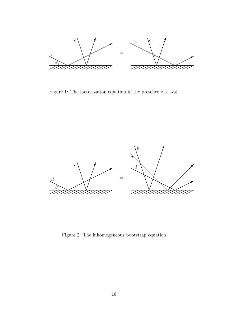
Diagramatically this corresponds to the equation in figure 1.

The presence of the wall breaks parity invariance, which - if true - would deman

d Scdab(θ) = Sdc

ba(θ). But restrictions of this kind can be genera ted, following the

argumentation originally due to Cherednik [3, 4]. In the limit, when the rapidity

of one of the particles vanishes, it is impossi ble to decide, whether it has or has

not hit the wall before scattering off a nother particle. This imposes the additional

conditions:

W aa (0)+Sb1a1

ba (θ) =0 Sa1b1ab (θ)W a1

a1(0),

W aa (0)0Sb1a1

ba (θ) =−Sa1b1ab (θ)W a1

a1(0). (3.8)

To complete the scheme, we still have to consider 3-particle scattering. Howev er if

equ.(3.7) is satisfied, we can always arrange rapidities, such th at all particles scatter

against each other, before ( or after ) they hit the wall. Therefore factorization

requires ±S(θ) to satisfy in additi on the usual Yang-Baxter equations

±S a′ b′

ab (θab)±S ac′

ac (θac)±S bc

bc(θbc) =± S b′c′

bc (θbc)±S a′ c

ac (θac)±S ab

ab(θab) . (3.9)

These equations are sufficient to determine the S- and W -matrices, unless th ey are

diagonal. In this case (3.7) are trivially satisfied and we requ ire more information

to determine them. Once an S-matrix posses a pole due to the propagation of a

bound state particle, one can formulate the so-called

4 Bootstrap equations

For simplicity we will in the sequel consider only diagonal S, W -matrices:

W ba(θ) = δb

aWa(θ) (4.10)

4

and similarly for the S-matrices. In this case equs.(3.7) and (3.8) are satisfied, if

0Sba(θ) =0 Sab(θ) =−Sab(θ) =+Sba(θ) =−Sba(θ) =+ Sab(θ). (4.11)

Here we used unitarity equ.(2.5), which implies W (0)2 = 1. Equ.(4.11) includes

constraints usually coming from parity invariance. As a result of this equation we

shall not distinguish anymore in the following between −S,0 S,+ S and solely refer

to them as S.

When particle c is a bound state of particles a and b one assumes in addition to

the Zamolodchikov algebra the validity of an operator product expansion involving

the operators representing those particles

Za

(

θ + iηbac +

iε

2

)

Zb

(

θ − iηabc −

iε

2

)

=iΓc

abZc(θ)

ε, (4.12)

where Γkij denotes the three particle vertex on mass-shell and ηc

ab are the so-called

fusing angles. Then multiplying this equation by Zd(θd), using equation (2.1) and

taking the limit ε → 0 leads to a nontrivial consistency condition, which is known

as the bootstrap equation [?]

Sdc(θ) = Sda(θ − iηbac) Sdb(θ + iηa

bc) . (4.13)

It states that scattering particle d against c is equivalent to scatter d against the

bound state a+b. Evidently there has to be an equation of this kind in the presence

of reflecting boundaries. Thus let us scatter particles a, b and d with rapidities

θ0 + iηbac + iε

2, θ0 − iηa

bc − iε2, θd > 0. We obtain by the same procedure as in the

previous subsection

Za

(

θ0 + iηbac +

iε

2

)

Zb

(

θ0 − iηabc −

iε

2

)

Zd(θd)Zw(0) = Sab

(

2θ0 + iηbac − iηa

bc

)

Sad

(

θ0d + iηbac +

iε

2

)

Sbd

(

θ0d − iηabc −

iε

2

)

Sad

(

θ0d + iηbac +

iε

2

)

Sbd

(

θ0d − iηabc −

iε

2

)

Wa

(

θa + iηbac +

iε

2

)

Wb

(

θb − iηabc −

iε

2

)

Wd(θd)

Zb

(

−θ0 + iηabc +

iε

2

)

Za

(

−θ0 − iηbac −

iε

2

)

Zd(−θd)Zw(0) .

5

On the other hand multiplying equation (4.12) by Zd(θd)Zw(0) and performing

similar operations we derive after taking the limit ε → 0, the bootstrap equation in

the presence of the wall

Sdc(θ0d) Sdc(θ0d)Wc(θc) = Wa(θa + iηbac)Wb(θb − iηa

bc) (4.14)

Sab(2θ0 + iηbac − iηa

bc)Sad(θ0d + iηbac)Sbd(θ0d − iηa

bc)Sad(θ0d + iηbac)Sbd(θ0d − iηa

bc).

Diagramatically we depict this situation in figure 2. Since the scattering matrix

satisfies the conventional bootstrap equation (4.13), our equation for W reduces to

Wc(θ) = Wa(θ + iηbac) Wb(θ − iηa

bc) Sab(2θ + iηbac − iηa

bc) (4.15)

which we call, due to the presence of the factor Sab(2θ0 + iηbac − iηa

bc), an inhomoge-

neous bootstrap equation.

The equations (3.7) and (4.14) also solve the analogous problem of factorized

scattering in the presence of two walls, since the two walls do not interfere with

each other.

5 The W -matrix

In this section, we shall discuss the solutions of the coupled equs. (4.15). The two

particle scattering matrices to be used in this paper always factorize into the form

S(θ) =∏

x{x}θ. Adopting our notation from [8], each of this block reads

{x}θ :=[x]θ

[−x]θ, (5.16)

with

[x]θ :=〈x + 1〉θ〈x − 1〉θ

〈x + 1 − B〉θ〈x − 1 + B〉θ(5.17)

and

〈x〉θ := sinh1

2

(

θ +iπx

h

)

. (5.18)

6

B is a function, which takes its values between 0 and 2 containing the dependence

on the coupling constant β of the Lagrangian field theory. h denotes the Coxeter

number of the underlying Lie algebra of the theory. The S-matrices possess further-

more the property to be invariant under B → 2 − B, that is under an interchange

of the strong and weak coupling regime.

Alternatively each block is equivalent to the following integral representation

{x}θ = exp

(

∫ ∞

0

dt

t sinh tfx,B(t) sinh

θt

iπ

)

(5.19)

where

fx,B(t) = 8 sinhtB

2hsinh

t

h

(

1 − B

2

)

sinh t(

1 − x

h

)

. (5.20)

Whilst (5.16) nicely exhibits the polestructure of the S-matrix, equation (5.19) is

sometimes more useful for explicit evaluations and we shall require this form below.

We might now expect that the W -matrix factorizes in an analogous fashion into

blocks as the S-matrix. Indeed we find a one-to-one correspondence between the

blocks of the W - and S-matrix:

W (θ) =∏

x

Wx(θ) . (5.21)

Similar as the S-matrix, the W -matrix factorizes further into subblocks

Wx(θ) =w1−x(θ)w−1−x(θ)

w1−x−B(θ)w−1−x+B(θ). (5.22)

As demanded by the unitarity (2.5) of the W -matrix we have

wx(θ) wx(−θ) = 1. (5.23)

Furthermore we shall verify the relations

wx−2h(θ) w−x(θ) = 1 (5.24)

wx(0) = w−h(θ) = 1 (5.25)

wx

(

θ +iyπ

2h

)

wx

(

θ − iyπ

2h

)

= wx+y(θ) wx−y(θ) (5.26)

wx(θ + iπ) = ηx(θ) wx(θ) (5.27)

7

where the function ηx(θ) satisfies individually the homogeneous bootstrap equation

ηx(θ + iηbac) ηx(θ − iηa

bc) = ηx(θ) . (5.28)

Notice that ηx(θ) does not contain any poles in the physical sheet 0 < θ < iπ. All

blocks converge to one in the asymptotic limit θ → 0, resulting from

limθ→∞

wx(θ) = 1 . (5.29)

It turns out that the function wx(θ) posses neither poles nor zeros in the physical

strip, such that no particle creation and absorption takes place in the wall. The ab-

sence of the poles and zeroes was expected from the assumpti on that the scattering

off the wall takes place in an elastic fashion.

We shall now compute some explicit examples of the W -matrix, starting with

th e

5.1 The Bullough-Dodd model

The BD-model [9] ( A(2)2 -affine Toda theory ) represents an integrab le quantum

field theory involving one type of scalar field only, which satisfies a relativistically

invariant equation in two dimensions. The model is ideal to illustrate the general

principles presented in the previous sections, since the particle, say A, emerges as

a bound state of itself, i.e. A + A → A is possible. Its classical Lagrangian is

obtainable from a folding [10, 11] of the D(1)4 -affine Toda theory, where the three

ro ots corresponding to the degenerate particles and the negative of the highest

root are identified. The resulting Dynkin diagram is the simplest example of a

non-simply laced one, containing the root α, which is related to the scalar field,

whose square length equals two and the root α0 = −2α, whose square length is

consequently eight. Then its classical Lagrangian density reads

L =1

2∂µφ∂µφ − m2

β2

(

2eβφ + e−2βφ)

, (5.30)

8

where m denotes the bare mass and β the coupling constant, which we assume to

be real to avoid the presence of solitons. For more details on the model we refer to

[12] and the references therein , but here we mainly want state the main properties

we are going to employ. The scattering matrix can be obtained by the above folding

procedure and it turns out to be [6]

SBD(θ) = {1}θ {2}θ . (5.31)

The Coxeter number of the BD-model equals three.

The scattering matrix satisfies the homogeneous bootstrap equation in the form

SBD(θ) = SBD (θ + ω) SBD (θ − ω) , (5.32)

with ω = iπ3

and consequently the inhomogeneous bootstrap eq uation acquires the

form

W (θ) = W (θ + ω) W (θ − ω) SBD(2θ) . (5.33)

Employing now Fourier transforms after taking the logarithm to solve such equa-

tions, we obtain

W (θ) = exp( ∫

dθ′ G(θ − θ′) ln S(2θ′))

, (5.34)

where the Green function G is given by

G(θ) = limη↑1

1

ω√

3

sinh(

2π3ω

(θ)η)

sinh(

π3(θ)η

) . (5.35)

The introduction of the parameter η is necessary to guarantee the convergen ce of

the Fourier transform. Employing now the integral representation for the blocks of

the S-matrix (5.19), we are lead to a factorization of the form (5.21) and (5.22),

where each of the sublocks wx(θ) is given by the integral representation

wx(θ) = exp

∫ ∞

0

dt

t sinh t

2 sinh(

1 + xh

)

t sinh 2θtiπ

1 − 2 cosh 2tωπ

. (5.36)

9

Solving the integral we obtain

wx(θ) =∞∏

l=0

Γ(

1 + (l + 1)ωπ

+ x2h

+ iθπ

)

Γ(

(l + 1)ωπ− x

2h− iθ

π

)

Γ(

(l + 1)ωπ− x

2h+ iθ

π

)

Γ(

1 + (l + 1)ωπ

+ x2h

− iθπ

)

sin((l+1)ω)sin ω

.

(5.37)

This equation exhibits nicely the pole structure of wx(θ), and therefore W (θ), and

can be used to prove the functional identities (5.23) - (5.29). The function η(θ),

which results as a shift of iπ in equation (5.27) takes on the form

ηx(θ) =∞∏

l=0

(

(l + 1)ωπ− x

2h− iθ

π

) (

−1 + (l + 1)ωπ

+ x2h

+ iθπ

)

(

1 + (l + 1)ωπ

+ x2h

− iθπ

) (

(l + 1)ωπ

+ x2h

+ iθπ

)

sin((l+1)ω)sin ω

(5.38)

and satisfies individually the homogeneous bootstrap equation

ηx(θ + iω) ηx(θ − iω) = ηx(θ) . (5.39)

ηx(θ) does not posses any poles in the physical sheet. Furthermore we derive from

(5.37) the functional equation

wx(θ + iω) wx(θ − iω) = wx(θ)〈x〉−2θ

〈x〉2θ

(5.40)

from which we infer the crucial identity for the blocks of the W-matrix

Wx(θ) = Wx(θ + iω) Wx(θ − iω){x}2θ . (5.41)

This equation demonstrates explicitly that the factorization of W occurs in a one-

to-one fashion with respect to the factorization of the S-matrix and we finally obtain

the solution for the W -matrix of the Bullough-Dodd model

W (θ) = W1(θ)W2(θ). (5.42)

Notice that this function posses neither poles nor zeros in the physical sheet .

10

5.2 The A(1)2 -affine Toda theory

The A(1)2 -affine Toda theory is the most simple example of an affine Toda theory

[13, 14] involving more than one particle. It contains two particles of equal masses

which are conjugate to each other, that is choosing complex scalar fields we have

φ∗1 = φ2. Its classical Lagrangian de nsity

L =1

2∂µφ∂µφ − m2

β2

(

eβ√

2φ2 + eβ√2(√

3 φ1−φ2) + e− β√

2(√

3 φ1+φ2))

(5.43)

possesses a ZZ3-symmetry, in the sense that it is left invariant under the transfor-

mation

φ →

e2πi3

n

e4πi3

n

φ n = 1, 2, 3 . (5.44)

From the three point couplings, which turn out to be C111 = −C222 = −i3βm2

and C112 = C221 = 0 or the application of the fusing rule of affine Toda theory

[15, 16, 8, 17] we obtain that the following processes are permitted

V1 + V1 → V2 = V1 (5.45)

V2 + V2 → V1 = V2 (5.46)

where we denote the particles by Vi with i = 1, 2. The scattering matrices are given

by

S11(θ) = S22(θ) = {1}θ (5.47)

S12(θ) = {2}θ. (5.48)

Here the blocks are again of the form (5.16) with h = 3. Where S11(θ) = S22(θ) have

poles at 2πi3

describing the processes (5.45) and (5.46), whereas S12(θ) has no poles

in the physical sheet. Furthermore, the scattering matrix satisfies the bootstrap

equations

Sl2(θ) = Sl1(θ + iω)Sl1(θ − iω) (5.49)

Sl1(θ) = Sl2(θ + iω)Sl2(θ − iω) (5.50)

11

for l = 1, 2, ω = iπ/3, together with the crossed versions of this. S ince the

scattering matrices involved satisfy the ordinary bootstrap equation s, the wall

bootstrap equations reduce to

W2(θ) = W1(θ + iω) W1(θ − iω) S11(2θ) (5.51)

W1(θ) = W2(θ + iω) W2(θ − iω) S22(2θ) . (5.52)

Together with equation (5.41) we notice that these equations are solved by

W1(θ) = W2(θ) = W1(θ) . (5.53)

Again W (θ) introduces no poles nor zeros in the physical sheet. The fact tha t

W1(θ) equals W2(θ) is a consequence of the mass degeneracy of the theory, which

is reflected by the automorphism of the Dynkin diagram [10, 11]. The folding

towards the Bullough-Dodd model introcuces an additional block in the W-

matrix, due to the identification of particle 1 and 2, in a similar fashion as for the

S-matrix.

5.3 The A(2)4 -affine Toda theory

The A(2)4 affine Toda theory is the most simple example of an affine Toda theory,

where the roots associated to the particles are connected by more than one lace on

the Dynkin diagram. It descibes two self-conjugate real scalar fields whose classical

mass ratio is m21 = (5 −

√5)/(5 +

√5)m2

2. The roots involved in this theory might

be constructed from a D(1)6 -affine Dynkin diagram, where the four roots forming the

two handles and the two roots which are connnected to the handles are identified.

The resulting roots are

α1 = −2√

2√5

(

sin2π

5, sin

π

5

)

and α2 =4√

2√5

(

sinπ

5cos

2π

5, sin

2π

5cos

π

5

)

(5.54)

12

where the root corresponding to the affinisation α0 is the negative of twice the sum

of this two roots. In terms of this vectors the Lagrangian density reads

L =1

2∂µφ∂µφ − m2

β2

(

eβα0·φ + 2eβα1·φ + 2eβα2·φ)

, (5.55)

from which we may compute the three point couplings C111 = C222 = 0 and C221 6=0, C112 6= 0 such that the following fusing processes are possible

V1 + V1 → V2 (5.56)

V2 + V2 → V1 (5.57)

V1 + V2 → V1 + V2 . (5.58)

The corresponding scattering matrices turn out to be

S11(θ) = {1}θ{4}θ (5.59)

S12(θ) = {2}θ{3}θ (5.60)

S22(θ) = {1}θ{2}θ{3}θ{4}θ. (5.61)

The Coxeter number h is five in this case. Here S11(θ) has a single pole with

negative residue at 3πi5

and one with positive residue at 2πi5

describing the process

(5.56). S12(θ) has single poles with negative residues at πi5, 2πi

5and single poles

with positive residue at 3πi5

, 4πi5

corresponding to (5.58). S22(θ) has a single pole

with negative residue at πi5, a single pole with positive residue at 4πi

5related the the

fusing (5.57) and double poles at 2πi5

3πi5

. The bootstrap equation are in this case

Sl2(θ) = Sl1(θ + iω)Sl1(θ − iω) (5.62)

Sl1(θ) = Sl2(θ + iω)Sl2(θ − iω) (5.63)

Sl1(θ) = Sl1(θ + 3iω)Sl2(θ + iω) (5.64)

Sl2(θ) = Sl2(θ − iω)Sl1(θ + 2iω) (5.65)

with l = 1, 2. Because of the previous equations, the wall bootstrap equations

reduce to

W2(θ) = W1(θ + iω) W1(θ − iω) S11(2θ) (5.66)

13

W1(θ) = W2(θ + iω) W2(θ − iω) S22(2θ) (5.67)

W1(θ) = W2(θ + iω) W1(θ − 3iω) S12(2θ) (5.68)

W2(θ) = W1(θ + 2iω) W2(θ − iω) S12(2θ) . (5.69)

Introducing the notation W11(θ) := W1(θ) , W22(θ) := W2(θ) and W12(θ) :=

W2(θ)/W1(θ) , these equations decouple and we are left with the problem to solve

Wij(θ) = Wij(θ + iω) Wij(θ − iω) Wij(θ + 3iω) Wij(θ − 3iω) Sij(2θ) . (5.70)

Again we utilise Fourier transforms after taking the logarithm and obtain

Wij(θ) = exp( ∫

dθ′ G(θ − θ′) ln Sij(2θ′))

, (5.71)

where the Green function G(θ) in this case is given by

G(θ) = limη↑1

1

ω sinh πθη

ω

sinh(

π3ω

(θ)η)

sin 2π3

+sinh

(

4π5ω

(θ)η)

sin ω + 3 sin 3ω+

sinh(

2π5ω

(θ)η)

sin 3ω + 3 sin 9ω

.

(5.72)

Employing now again the integral representation for the S-matrix we obtain the

following integral representaion for the building blocks of the W-matrix

wx(θ) = exp(

I 2π3(θ) + Iω(θ) + I3ω(θ)

)

, (5.73)

whith

Ia(θ) =1

5 − 6 sin2 a

∫ ∞

0

dt

t sinh t

2 sinh(

1 + xh

)

t sinh 2θtiπ

cos a − 2 cosh 2tωπ

. (5.74)

Solving the integral gives

wx(θ) =∞∏

l=0

Γ(

1 + (l + 1)ωπ

+ x2h

+ iθπ

)

Γ(

(l + 1)ωπ− x

2h− iθ

π

)

Γ(

(l + 1)ωπ− x

2h+ iθ

π

)

Γ(

1 + (l + 1)ωπ

+ x2h

− iθπ

)

Pl

. (5.75)

with

Pl =sin

(

(l + 1)2π3

)

sin(

π3

) +sin

(

(l + 1)π5

)

2 sin(

π5

) (

5 − 6 sin2(

π5

)) +sin

(

(l + 1)3π5

)

2 sin(

3π5

) (

5 − 6 sin2(

3π5

))

(5.76)

14

Again this equation is useful to extract the polestructure and to prove the identities

(5.23) - (5.29). The function ηx(θ) is n ow given by

ηx(θ) =∞∏

l=0

(

(l + 1)ωπ− x

2h− iθ

π

) (

−1 + (l + 1)ωπ

+ x2h

+ iθπ

)

(

1 + (l + 1)ωπ

+ x2h

− iθπ

) (

(l + 1)ωπ

+ x2h

+ iθπ

)

Pl

, (5.77)

satisfying the homogeneous bootstrap equation and having no poles in the physica

l sheet. Further we derive the relation

wx(θ + iω) wx(θ − iω)wx(θ + 3iω)wx(θ − 3iω) =〈x〉−2θ

〈x〉2θ

(5.78)

from which we deduce

Wijx(θ) = Wijx

(θ + iω)Wijx(θ − iω)Wijx

(θ + 3iω)Wijx(θ − 3iω){x}2θ. (5.79)

Comparision with equation (5.70) now demonstrates that the W -matrix again fac-

torizes in a one-to-one fashion with respect to the scattering matrix and we finally

obtain the W -matrix for the A(4)2 -affine Toda theory

W1(θ) = W1W4 (5.80)

W2(θ) = W1W2W3W4 (5.81)

From the property of the function wx(θ) we note again that the physical sheet is

free of singularities.

6 Conclusions

We have demonstrated how to formulate factorization equations and in particu-

lar the inhomogeneous bootstrap equations by employing an extended version of

Zamolodchikov’s algebra. Whereas in the absence of reflecting boundaries such

equations could be utilised to construct the two particle scattering matrix, now

they are sufficient to determine the W -matrix, which encodes the scattering of a

particle off the wall. For all cases investigated W (θ) does posses neither poles nor

15

zeros in the physical sheet, such that the wall does not create or absorb any parti-

cles. This feature is made transparent by expressing W (θ) as infinite products of Γ

functions. A ctually the structure is very similar to the one found for the minimal

two pa rticle form factors F (θ) [18, 12].

References

[1] C.N. Yang, Phys. Rev. Lett. 19 (1967) 1312; R.J. Baxter, Exactly Solved Models

in Statistical Mechanics (Academic Press, London, 1982 ).

[2] A.B. Zamolodchikov and Al. B. Zamolodchikov, Ann. Phys. 120 (1979) 253.

[3] I.V. Cherednik Theor. and Math. Phys. 61 1984 977.

[4] I.V. Cherednik, Notes on affine Hecke algebras. 1. Degenerated affine Hecke

algebras and Yangians in mathematical physics., BONN-HE-90-04 .

[5] E.K. Sklyanin J. Math. Phys. A21 (1988) 2375.

[6] A.E. Arinshtein, V.A. Fateev and A.B. Zamolodchikov, Phys. Lett. 87B (1979)

389.

[7] R. Koberle and J.A. Swieca, Phys. Lett. 86B (1979) 209; A.B. Zamolodchikov,

Int. J. Mod. Phys. A3 (1988) 743; V. A. Fateev and A.B. Zamolodchikov, Int.

J. Mod. Phys. A5 (1990) 1025.

[8] A. Fring and D.I. Olive, Nucl. Phys. B379 (1992) 429.

[9] R.K. Dodd and R.K. Bullough, Proc. Roy. Soc. Lond A352 (1977), 481.

[10] S. Helgason, Differential Geometry and Symmetric Spaces (Academic Press,

London, 1978 ).

[11] D.I. Olive and N. Turok, Nucl. Phys. B215 [FS7] (1983) 470.

16

[12] A. Fring, G. Mussardo and P. Simonetti, Form Factors of the Elementary Field

in the Bullough-Dodd Model, ISAS/EP/92/208, USP-IFQSC/TH/9 2-51.

[13] A.V. Mikhailov, M.A. Olshanetsky and A.M. Perelomov, Comm. Math. Phys.

79 (1981), 473; G. Wilson, Ergod. Th. Dyn. Syst. 1 (1981) 361; D.I. Olive and

N. Turok, Nucl. Phys. B257 [FS14] (1985) 277.

[14] H. W. Braden, E. Corrigan, P. E. Dorey and R. Sasaki, Phys. Lett. B227 (1989)

411; H. W. Braden, E. Corrigan, P. E. Dorey and R. Sasaki, Nucl. Phys. B338

(1990) 689.

[15] P.E. Dorey, Nucl. Phys. B358 (1991) 654; P.E. Dorey, Nucl. Phys. B374 (1992)

741.

[16] A. Fring, H.C. Liao and D.I. Olive, Phys. Lett. B266 (1991) 82.

[17] H.W. Braden, J. Phys. A25 (1992) L15.

[18] A. Fring, G. Mussardo and P. Simonetti, Nucl. Phys. B393 (1993) 413.

17

�������������������������������� ��������������������������������

=

��������

BB

BB

BBB

��������

BB

BBB

BB

�����������*

HHHHH

�����*

HHHHHHHHHHH

b

θb

a ab

Figure 1: The factorization equation in the presence of a wall

�������������������������������� ��������������������������������

=

��������

BB

BB

BBB

�����������*

HHHHHd

θd

c

�����*

HHHHHHHHHHH

��

��

����

@@

@@

@@

@@

@@

������������

BB

BBB

BBB

BBB

d

a

b

Figure 2: The inhomogeneous bootstrap equation

18