Orderings for Factorized Sparse Approximate Inverse Preconditioners

ORDERINGS FOR FACTORIZED SPARSE APPROXIMATEINVERSE PRECONDITIONERS∗

MICHELE BENZI† AND MIROSLAV TUMA‡

SIAM J. SCI. COMPUT. c© 2000 Society for Industrial and Applied MathematicsVol. 21, No. 5, pp. 1851–1868

Abstract. The influence of reorderings on the performance of factorized sparse approximateinverse preconditioners is considered. Some theoretical results on the effect of orderings on the fill-inand decay behavior of the inverse factors of a sparse matrix are presented. It is shown experimentallythat certain reorderings, like minimum degree and nested dissection, can be very beneficial. Thebenefit consists of a reduction in the storage and time required for constructing the preconditioner,and of faster convergence of the preconditioned iteration in many cases of practical interest.

Key words. sparse linear systems, sparse matrices, preconditioned Krylov subspace methods,graph theory, orderings, decay rates, factorized sparse approximate inverses, incomplete biconjuga-tion

AMS subject classifications. Primary, 65F10, 65N22, 65F50; Secondary, 15A06

PII. S1064827598339372

1. Introduction. We consider the solution of sparse linear systems Ax = b bypreconditioned iterative methods, where the preconditioners are sparse approximateinverses of A. Such preconditioners have particular interest from the point of viewof parallel computation since their application at each step of an iterative methodrequires only sparse matrix–vector products, which are relatively easy to parallelize.Moreover, sparse approximate inverse preconditioners often succeed in solving difficultproblems for which ILU-type methods fail, and therefore they can be useful even onsequential computers. A comprehensive survey of sparse approximate inverse precon-ditioners, together with the results of extensive numerical tests aimed at assessing theperformance of the various methods, can be found in [6]. One of the conclusions ofthat study was that factorized forms, in which the approximate inverse is the productof two sparse triangular matrices, tend to perform better than nonfactorized ones inthe sense that they often deliver better convergence rates for the same amount ofnonzeros in the preconditioner. Factorized approximate inverses are also much lessexpensive to compute than other forms, at least in a sequential environment. As men-tioned in [6], another potential advantage of the factorized approach is the fact thatsuch preconditioners are sensitive to the ordering of the equations and unknowns. In-deed, for a sparse matrix A the amount of inverse fill, which is defined as the numberof structurally nonzero entries in the inverse triangular factors, is strongly dependenton the ordering of A. In contrast, the inverse A−1 is usually full, regardless of the

∗Received by the editors May 26, 1998; accepted for publication (in revised form) December12, 1998; published electronically April 28, 2000. This work was performed by an employee of theU.S. Government or under U.S. Government contract. The U.S. Government retains a nonexclusive,royalty-free license to publish or reproduce the published form of this contribution, or allow othersto do so, for U.S. Government purposes. Copyright is owned by SIAM to the extent not limited bythese rights.

http://www.siam.org/journals/sisc/21-5/33937.html†Scientific Computing Group (CIC-19), MS B256, Los Alamos National Laboratory, Los Alamos,

NM 87545 ([email protected]). The work of this author was supported in part by Department of Energygrant W-7405-ENG-36 with Los Alamos National Laboratory.

‡Institute of Computer Science, Academy of Sciences of the Czech Republic, Pod vodarenskouvezı 2, 182 07 Prague 8, Czech Republic ([email protected]). The work of this author was supportedby Grant Agency of the Czech Academy of Sciences grant 2030706 and by Grant Agency of the CzechRepublic grant 205/96/0921.

1851

1852 MICHELE BENZI AND MIROSLAV TUMA

ordering chosen. In this paper we focus on the factorized sparse approximate inversepreconditioner AINV based on incomplete (bi)conjugation, developed in [2], [4]. Asalready noted in [4], this algorithm can benefit from the minimum degree ordering,which tends to reduce the amount of inverse fill without negatively impacting the rateof convergence. Here we present results with several orderings in addition to minimumdegree. We consider the effect of reorderings from the point of view of the induced fillin the inverse factors using tools from graph theory, and we obtain some insight intothe concomitant effects on the decay of the entries in the inverse factors. We concludethat reorderings, particularly minimum degree and nested dissection, can significantlyenhance the performance of the AINV preconditioner. We also look briefly at otherapproximate inverse techniques, showing that the effect of ordering can be quite differ-ent on different methods. In the present study we restrict our attention to symmetricpermutations of the coefficient matrix A, i.e., of the form PTAP for a permutationmatrix P . These permutations do not alter the spectrum of A. Also, we are mostlyinterested in solving linear systems arising from the discretization of partial differen-tial equations, which typically give rise to matrices which are structurally symmetricor nearly so, and nonsymmetric permutations would destroy the symmetry. If A isstructurally symmetric the reorderings are based on the (undirected) graph associatedwith the structure of A; otherwise, the structure of A+AT is used. See [13], [18], [36]for basic material on sparse matrix orderings.

This paper complements a recent independent study by Bridson and Tang [7], whoalso considered the effect of ordering on AINV. Our main conclusions are similar tothose reached in [7]; however, several of our results are not found in [7], and conversely,several orderings and new heuristics not considered here can be found in [7]. Wherewe overlap, our results and those in [7] are in good agreement. See also [17] for relatedwork.

2. The AINV algorithm. The AINV algorithm [2], [4], [6] constructs a fac-torized sparse approximate inverse of the form

M = ZD−1WT ≈ A−1,

where Z,W are unit upper triangular matrices and D is diagonal. The approximateinverse factors Z and W are sparse approximations of the inverses of the L and Ufactors in the LDU decomposition of A. The AINV algorithm computes Z,W andD directly from A by means of an incomplete biconjugation process, in which smallelements are dropped to preserve sparsity. In order to describe the procedure, let aTiand cTi denote the ith row of A and AT , respectively (i.e., ci is the ith column of A).Also, let ei denote the ith unit basis vector. The basic A-biconjugation procedure canbe written as follows.

Algorithm 2.1. Biconjugation algorithm.(1) Let w

(0)i = z

(0)i = ei (1 ≤ i ≤ n)

(2) For i = 1, 2, . . . , n do(3) For j = i, i+ 1, . . . , n do

(4) p(i−1)j := aTi z

(i−1)j ; q

(i−1)j := cTi w

(i−1)j

(5) End do(6) if i = n go to (11)(7) For j = i+ 1, . . . , n do

(8) z(i)j := z

(i−1)j −

(p(i−1)j

p(i−1)i

)z(i−1)i ; w

(i)j := w

(i−1)j −

(q(i−1)j

q(i−1)i

)w

(i−1)i

ORDERINGS FOR FACTORIZED INVERSE PRECONDITIONERS 1853

(9) End do(10) End do

(11) Let zi := z(i−1)i , wi := w

(i−1)i and pi := p

(i−1)i , for 1 ≤ i ≤ n. Return

Z = [z1, z2, . . . , zn], W = [w1, w2, . . . , wn], and D = diag(p1, p2, . . . , pn).Sparsity is preserved by dropping in the z- and w-vectors after the updates at step

(8). If A = AT , then Z =W and the columns of Z are (approximately) A-conjugate.The incomplete procedure is well defined, i.e., no breakdown can occur, if A is anH-matrix. In the general case, diagonal shifts may be necessary in order to preventbreakdowns. See [2], [4], [6] for a detailed study of this algorithm and comparisonswith other preconditioners.

3. Structural considerations. In this section we review the effect of orderingson the amount of fill occurring in the inverse triangular factors of a sparse matrix A.See also [7] for a treatment along similar lines.

The inverse of a sparse irreducible matrix is structurally full [12], [19], and thisproperty is obviously invariant under permutations. However, A−1 may be repre-sentable as the product of two sparse triangular matrices. We are interested in find-ing permutations of A such that the inverse triangular factors Z,W of A preserve agood deal of sparsity. For example, consider an irreducible matrix partitioned in thefollowing block form:

A =

A1 0 B1

0 A2 B2

C1 C2 A3

.

Then A−1 is full, but the inverse triangular factors of A have the same block structureas the lower and upper block triangular parts of A. In particular, fill-in can occur onlyinside the nonzero blocks. If a similar structure is imposed on the diagonal blocks A1

and A2, as is done in nested dissection, then it is clear that the inverse factors willretain a considerable degree of sparsity.

Let A be an unsymmetric n× n matrix that has a factorization A = LU withoutpivoting. Let G(A) = (V (A), E(A)) be the directed graph of the matrix A, whereV (A) = 1, . . . , n is the vertex set and E(A) is the set of edges 〈i, j〉 with i, j suchthat aij = 0. Let x ∈ V (A). The closure clG(A)(x) of x in G(A) is the set of verticesof G(A) from which there are paths to x. The structure of a vector v is defined asStruct(v) = i|vi = 0. In the following we will state results for the factor L−1.Similar results hold, of course, also for the factor U−1. These results were given in[19], [20]. The usual no cancellation assumption is made throughout. We denote byL−1(∗, i) the ith column of L−1.

Proposition 3.1. Struct(L−1(∗, i)) = clG(L)(i).Let G(L) denote the transitive reduction of the directed acyclic graph (dag)

G(L). This is a graph with a minimal number of edges which satisfies the followingcondition: G(L) has a directed path from i to j if and only if G(L) has a directedpath from i to j. Then the following result holds [20].

Proposition 3.2. Struct(L−1(∗, i)) = clG(L)(i).We mention two simple consequences of this relation.Proposition 3.3. Assume that clG(L)(i) ∩ clG(L)(j) = ∅. Then

Struct(L−1(∗, i)) ∩ Struct(L−1(∗, j)) = ∅.Proposition 3.4. Let K = clG(L)(i)∩ clG(L)(j). If K = ∅, then all the entries

below the main diagonal in L−1(K,K) are nonzero.

1854 MICHELE BENZI AND MIROSLAV TUMA

Another way to phrase this structural characterization is by saying that the (i, j)element of W = L−T is nonzero if and only if j is an ancestor of i in the eliminationtree; see [7]. Incidentally, this characterization is considerably simpler than the onegiven in [4], which was intended mainly to serve as a guide for the extension ofthreshold pivoting strategies to the biconjugation process.

The construction of factorized approximate inverse preconditioners is naturallyinfluenced by the inverse fill. Orderings that cause relatively low inverse fill can beexpected to result in more sparse approximate inverse factors and possibly in fastercomputation of the preconditioner. On the other hand, it is difficult to predict theimpact that reorderings obtained using unweighted graph information only will haveon the rate of convergence of the preconditioned iteration; see the next section for adiscussion.

In any event, it makes sense to attempt to keep the number of nonzeros in L−1

small, i.e., to try to minimize for each j, with respect to the ordering, the sum∑i<j

|clG(L)(i) ∩ clG(L)(j)|.(3.1)

This sum represents the overlaps between the closure of vertex j and the remainingclosures in the elimination dag. Finding an ordering that minimizes this sum wouldresult in overlaps between individual closures which are as small as possible or, inother words, in an elimination dag which is as bushy as possible. Since the inverse fillcorresponds to the closures of the vertices, a bushy dag can be expected to provideless inverse fill. The combinatorial optimization problem (3.1) has close links tothat of finding orderings which minimize the height of the elimination tree, which isimportant in the context of parallel sparse elimination. Previous work in this fieldwas targeted at structurally symmetric problems and attempted to restructure theelimination tree so as to reduce its height as much as possible; see [23], [26], [30], and[31]. The techniques proposed in these papers provide as a side effect a decrease inthe overlap between closures of the graph vertices. Note that the problem of findingorderings which result in elimination trees of minimum height for general graphs isNP-hard; see [35].

To illustrate the effect of ordering on the inverse fill-in, consider a matrix (sym-metric, for simplicity) before and after the reverse Cuthill–McKee (RCM) reordering.This reordering naturally tends to make the sums (3.1) rather large. Therefore a largeamount of inverse fill is to be expected since this is given by the sum of the overlapsof the closures of the vertices. Figure 3.1 shows the patterns of the matrix and theinverse of its factor L. Figure 3.2 shows the patterns of the matrix and the inverse ofL after RCM reordering. The inverse factor is much more dense in the second case.

Hence, we can expect that reorderings aimed at reducing the envelope or the bandwill tend to make the inverses of the triangular factors rather dense. Therefore, theRCM-like orderings do not seem to be advantageous as reordering options before thefactorized approximate inverse construction. Minimum degree and nested dissectionorderings are in principle more acceptable as reorderings for computing factorized ma-trix inverses. They provide more bushy elimination trees (or dags) resulting, typically,in less fill-in in the inverse factors. These orderings, particularly nested dissection, canalso be used to introduce parallelism in the computation of the AINV preconditioner.

One natural choice of an ordering which keeps the elimination tree reasonablyshort is nested dissection. It is known that for every graph there exists a nesteddissection ordering with minimal separators which produces an elimination tree of

ORDERINGS FOR FACTORIZED INVERSE PRECONDITIONERS 1855

∗ ∗ ∗ ∗∗ ∗ f f

∗ ∗ ∗∗ ∗ f

∗ f ∗ f ∗ f∗ ∗ ∗∗ ∗ f

∗ ∗ ∗∗ ∗ f

∗ f ∗ f ∗ ∗∗ f f ∗ ∗

∗∗ ∗

∗∗ ∗

∗ ∗ ∗ ∗ ∗∗∗ ∗

∗∗ ∗

∗ ∗ ∗ ∗ ∗∗ ∗ ∗ ∗ ∗ ∗ ∗ ∗ ∗ ∗ ∗

Fig. 3.1. Patterns of the matrix A (left) and of L−1, the inverse of its lower triangular factor(right). Stars denote matrix nonzeros; f is used to denote filled positions in L.

∗ ∗∗ ∗

∗ ∗ ∗∗ ∗ ∗

∗ ∗ ∗ ∗∗ ∗ ∗

∗ ∗∗ ∗ ∗ ∗

∗ ∗ ∗∗ ∗ ∗

∗ ∗

∗∗

∗ ∗∗ ∗

∗ ∗ ∗ ∗ ∗∗ ∗ ∗ ∗ ∗ ∗

∗∗ ∗ ∗ ∗ ∗ ∗ ∗ ∗∗ ∗ ∗ ∗ ∗ ∗ ∗ ∗ ∗∗ ∗ ∗ ∗ ∗ ∗ ∗ ∗ ∗ ∗∗ ∗ ∗ ∗ ∗ ∗ ∗ ∗ ∗ ∗ ∗

Fig. 3.2. Patterns of the matrix A (left) and of L−1, the inverse of its lower triangular factor(right) after the RCM reordering.

minimum height; see [31]. However, finding a nested dissection ordering with minimalseparators that produces an elimination tree of minimum height is also NP-hard.Next, we state a simple result for the five-point formula discretization of a second-order elliptic partial differential equation with Dirichlet boundary conditions on atwo-dimensional regular k × k grid. Note that the dimension of A is k2.

Theorem 3.1. Consider the matrix A from a k × k regular grid problem withthe nested dissection ordering. The number of nonzeros in the inverse factor L−1 isO(k3). The number of nonzeros in the inverse factor with the (reverse) Cuthill–McKeeordering is O(k4).

Proof. Consider first nested dissection of a naturally ordered grid. Without lossof generality we may assume that k = 2l − 1 for some l ≥ 2. Hence, the number oflevels in the separator tree is 2(l− 1) + 1. We will count nonzeros in columns of L−1

by levels in this tree. Columns corresponding to vertices of the first separator in thefirst level contribute k2/2 +O(k) nonzeros. Nodes in the next two separators of thesecond level contribute together 2(k(k/2) + k2/(2 · 22)) + O(k) nonzeros. There are2s−1 separators at the level s. In general, vertices in the separators at the sth levelcontribute 2s−1(as + bs) +O(k), where

as =

(k +

k

2+

k

2+

k

4+

k

4+ · · ·+ k

2s2−2

+k

2s2−2

+k

2s2−1

+k

2s2−1

)k

2s2

1856 MICHELE BENZI AND MIROSLAV TUMA

Table 3.1Inverse fill for regular grid problem, k = 100, various orderings.

Lexicographic RCM Min. deg. Nested diss. Red-black|L−1| 50,005,000 50,005,000 3,190,637 2,737,694 25,742,649

and bs = k2/2s+1 for s even;

as =

(k +

k

2+

k

2+

k

4+

k

4+ · · ·+ k

2s+12 −2

+k

2s+12 −2

+k

2s+12 −1

)k

2s+12 −1

and bs = k2/2s for s odd. Note that as and bs count nonzeros in rows correspondingto previous levels of separators up to the (s− 1)th level and nonzeros in rows of theseparator vertices from the sth level, respectively, in the submatrix of L−1 determinedby vertices from the separators considered so far. It is easy to see that summing asand bs separately over O(log2 k) levels we get O(k3) behavior for both sums.

(Reverse) Cuthill–McKee ordering of the grid results in a straight elimination treeof depth equal to k2. This implies O(k4) number of nonzeros in L−1.

More specifically, the inverse fill for the (reverse) Cuthill–McKee ordering isn(n+1)

2 , where n = k2; it is straightforward to see that the same holds for the lex-icographical ordering. For the red-black ordering, the inverse fill is approximatelyn(n+1)

4 .

As an illustration, we report in Table 3.1 the number of nonzeros in L−1 for afew orderings and k = 100.

4. Decay rates. In the previous section we showed that certain orderings resultin inverse triangular factors which preserve a good deal of sparsity. These orderingsare attractive from the point of view of computing a factorized sparse approximateinverse because intuitively they can be expected to result in significant savings in theinverse factorization process, both in time and space. Furthermore, one might expectthat it should be easier to find a good sparse approximation to a sparse inverse factorthan to a dense one. However, a weakness of these arguments is that the results inthe previous section are purely structural and give little insight into the quality of theapproximate inverse factors, which depends on the numerical values of the entries. Inother words, the structural results cannot tell the whole story since they disregardthe magnitude of the nonzeros and in particular their decay behavior, which is crucialin practice since, in the most effective algorithms, sparsity in the inverse factors ispreserved by applying a drop strategy based on value rather than on position.

The decay behavior of the entries of the inverse of a sparse matrix has beeninvestigated by several authors; see, for instance, [11], [15], [32], [34]. Most resultsconcern the case of symmetric banded matrices, but extensions to more general casesalso exist. Given an even integer m, a matrix A = (aij) is called m-banded if aij = 0for |i − j| > m/2. A well-known result by Demko, Moss, and Smith [11] gives anexponentially decaying upper bound for the entries of the inverse of a symmetricpositive definite (SPD) m-banded matrix A. Let a and b denote the smallest andlargest eigenvalue of A, respectively. Let κ = b

a denote the spectral condition numberof A. Set

q = q(κ) :=

√κ− 1√κ+ 1

ORDERINGS FOR FACTORIZED INVERSE PRECONDITIONERS 1857

and λ := q2/m. Also, set K0 := (1 +√κ)2/(2aκ). If B = (bij) denotes the inverse of

A, then Demko, Moss, and Smith showed that

|bij | ≤ Kλ|i−j|,(4.1)

where K := maxa−1,K0. For extensions and refinements of this result, see [15],[34].

Hence, the entries of A−1 are bounded in an exponentially decaying manner awayfrom the main diagonal, along each row and column. The rate of decay is governedby the extreme eigenvalues a and b of A, and by the bandwidth m. Decay canbe expected to be fast for matrices which are well conditioned and have a smallbandwidth; otherwise it can be very slow. While the constant K is independent ofm, symmetric permutations aimed at reducing the bandwidth can be used to reducethe value of λ. Hence, it may be possible to increase the rate of decay away from themain diagonal in the inverse by first applying a band-reducing permutation, such as(reverse) Cuthill–McKee. Since symmetric permutations do not affect the eigenvalues,the constant K is unchanged. Also notice that because (PTAP )−1 = PTA−1P forany permutation matrix P , applying a band-reducing permutation merely amountsto a redistribution of the entries of the inverse. This redistribution tends to move thelarger off-diagonal entries of A−1 near the main diagonal and the smaller ones awayfrom it. Of course, because the result by Demko, Moss, and Smith merely providesan upper bound (and a rather loose one in many cases), this need not always bethe case. However, if we want to compute a banded approximation to A−1, then itis clear that an ordering like RCM should be used, whereas orderings which resultin a large bandwidth, like minimum degree or nested dissection, should be avoided.In contrast, if an adaptive strategy is used to compute a sparse approximate inversein nonfactorized form, then the ordering is largely immaterial; see the numericalexperiments in the following section.

But what about factorized approximate inverses? The decay behavior of the en-tries in the inverse triangular factors of a sparse matrix does not seem to have beeninvestigated before. Yet, it is easy to see that the entries in the inverse Cholesky fac-tor of a banded SPD matrix also obey an exponentially decaying bound away fromthe main diagonal. This simple result is formalized in the following theorem. HereA = LLT is the Cholesky factorization of A (with L lower triangular) and we letZ = (zij) = L−T . Note that this matrix is equal to ZD−1/2, where now Z and D arethe output of the A-conjugation process on which the AINV algorithm is based. Also,the constants K and λ are defined as in the statement of the result (4.1) by Demko,Moss, and Smith.

Theorem 4.1. Let A be SPD and m-banded. Suppose that max1≤i≤naii = 1.Then for all i, j with j > i, the entries zij in Z = L−T satisfy the following upperbound:

|zij | ≤ K1λj−i,(4.2)

where K1 = K 1−λm

1−λ .

Proof. Let A−1 = B = (bij) and L = (lij). Notice that lij = 0 for i < j and

for i − j > m. From Z = L−T = A−1L we find that zij =∑j+m−1

k=j biklkj for i ≤ j.Therefore

|zij | ≤j+m−1∑k=j

|bik||lkj | ≤ K

j+m−1∑k=j

λk−i|lkj |,

1858 MICHELE BENZI AND MIROSLAV TUMA

where the second inequality is a consequence of the upper bound (4.1) on the entriesof B = A−1. Now we observe that the assumption max1≤i≤naii = 1 implies |lij | ≤ 1for all i, j, since |lij | ≤ √

aii (see [21, p. 147]). Hence,

|zij | ≤ K(λj−i + λj−i+1 + · · ·+ λj−i+m−1) = Kλj−i(1 + λ+ λ2 + · · ·+ λm−1)

from which the result immediately follows.Hence, the entries in Z are bounded in an exponentially decaying manner away

from the main diagonal along rows. This result can be generalized to some extent tononsymmetric problems using results from [11], [15], and [34]. For special classes ofmatrices something more precise can be said for the decay in the inverse factors: forinstance, in the M-matrix case it is easily seen that the entries of Z decay faster thanthe corresponding entries of A−1. This cannot be inferred from the bound (4.2) since0 < λ < 1 implies 1−λm

1−λ > 1 and therefore K1 > K. We recall that an M-matrix

A = (aij) is a matrix such that aij ≤ 0 for i = j and B = A−1 ≥ 0, i.e., bij ≥ 0 forall i, j. Furthermore, bij > 0 for all i, j if A is irreducible. Now, in the identity

zij = bij ljj +

j+m−1∑k=j+1

biklkj

the second summand on the right-hand side is nonpositive (negative if A is irreducible)because the off-diagonal entries of L are also. It follows that zij ≤ bij ljj , and if Ais normalized so that max1≤i≤naii = 1, then zij ≤ bij , the inequality being strictprovided that A is irreducible. Notice that this property does not require A to bebanded (i.e., m can be arbitrary). If A is banded, then we can conclude that theentries in the inverse Cholesky factor satisfy an exponentially decaying upper boundthat is at least as small as the one for the entries of A−1, and the actual decay rate isat least as fast as for A−1 (faster if A is irreducible). We mention that refined boundsfor the entries of the inverses of M-matrices can be found in [15] and [34].

This result may provide (for the class of M-matrices) a justification of the observedfact [5], [6] that factorized approximate inverses often provide better approximationsthan nonfactorized forms: because the entries in the inverse factors decay more rapidlythan the entries in A−1, it is easier to approximate L−1 with a sparse matrix than toapproximate A−1.

Concerning the normalization condition max1≤i≤naii = 1 used to derive ourresults, it is easy to see by examples that it is essential. In order to enforce sucha condition, it is clearly sufficient to divide A by its largest diagonal entry. Whilethe spectral condition number and the bandwidth (and therefore λ) are unaffectedby this normalization, the constant K is altered. Indeed, K will be increased if thelargest diagonal entry of A (prior to the normalization) is greater than 1. However,the qualitative behavior is the same.

Some insight on the effect of reorderings on the decay behavior of the entriesof the inverse factors is given by the following argument, which is adapted froman observation by Meurant concerning the effect of ordering on sparse incompleteCholesky factorizations [33]. Let Z be the inverse Cholesky factor of A, and let Zbe the inverse Cholesky factor of A := PTAP , where P is a permutation matrix.Denoting by ‖ · ‖F the Frobenius matrix norm, we have

‖Z‖F =√trace(ZZT ) =

√trace(A−1) =

√trace(A−1) = ‖Z‖F .

ORDERINGS FOR FACTORIZED INVERSE PRECONDITIONERS 1859

This means that an ordering which preserves sparsity in the inverse factors, like nesteddissection, will also result in nonzero entries which are larger, on the average, thanthose corresponding to an ordering which results in a high amount of fill, like reverseCuthill–McKee. With such an ordering, the use of a drop tolerance in an incompleteinverse factorization scheme (such as AINV) could in principle be problematic. Toosmall a drop tolerance could result in unacceptably high fill; limiting the number ofnonzeros accepted in each column of the approximate inverse factor (in an ILUT-likefashion) could lead to the dropping of many large entries, resulting in a very poorapproximation to the inverse. Increasing the drop tolerance may again lead to thedropping of too many large entries. In contrast, the quality of the preconditioner canbe more easily tuned if the entries in the inverse factors decay smoothly away fromthe main diagonal, and a dual threshold approach becomes viable. Notice that thissituation is not specific to factorized approximate inverse preconditioners: exactlythe same argument applies to standard ILU-type preconditioners. In particular, thissuggests a possible explanation of the generally poor performance of minimum degreefor ILU(0) and ILUT preconditioning (see [3], [14]).

Hence, we face the following dilemma: graph-theoretical considerations suggestthe use of orderings that will cause a small amount of inverse fill, like nested dissectionor minimum degree, whereas a look at the decay rates suggests that we use band-reducing orderings (like RCM), which cause large amounts of inverse fill but hopefullyresult in faster decay. As we shall see in the next section, it turns out that RCM isgenerally not a good ordering for factorized approximate inverses, whereas nesteddissection and minimum degree perform quite well, provided that the number ofnonzeros in each column (or row) of the inverse factors is not subject to any a prioriupper bound. It appears that for many problems, many of the nonzero entries inthe inverse factors corresponding to inverse fill-reducing orderings remain small inabsolute value, although they must be larger, on the average, than those correspondingto orderings leading to dense inverse factors.

We illustrate these points with some simple numerical examples computed usingMATLAB. Consider the tridiagonal (2-banded) irreducible M-matrix

A =

1 −1/4−1/4 1 −1/4

−1/4 1 −1/4−1/4 1 −1/4

−1/4 1

.

The upper triangular part of A−1 (rounded to four places) is1.0718 0.2872 0.0769 0.0205 0.0051

1.1487 0.3077 0.0821 0.02051.1538 0.3077 0.0769

1.1487 0.28721.0718

and the inverse factor is

Z = L−T =

1.0000 0.2582 0.0690 0.0185 0.0050

1.0328 0.2760 0.0739 0.01981.0351 0.2773 0.0743

1.0353 0.27741.0353

,

1860 MICHELE BENZI AND MIROSLAV TUMA

showing that the entries of Z are smaller than the corresponding entries of A−1. Therate of decay in A−1 is governed by the following quantities: K = K0 = 2.3401 andλ = 0.2277. The decay bounds Kλp, 0 ≤ p ≤ 4, are

[2.3401, 0.5329, 0.1214, 0.0276, 0.0063].

In this case the decay rate predicted by (4.1) is rather pessimistic, although theestimate becomes more accurate far from the main diagonal.

If a two-domain decomposition is applied to A, the permuted matrix is

A =

1 −1/4 0 0 0−1/4 1 0 0 −1/40 0 1 −1/4 −1/40 0 −1/4 1 00 −1/4 −1/4 0 1

.

The corresponding inverse factor is

Z =

1.0000 0.2582 0 0 0.0716

1.0328 0 0 0.28641.0000 0.2582 0.2864

1.0328 0.07161.0742

.

There are 15 nonzeros in Z and 11 in Z. Note that ‖Z‖2F = ‖Z‖2

F = 5.5949 =

trace(A−1) = trace(A−1). The elements in Z are larger, on the average, than those inZ. Note, however, that the growth is confined to entries in the last column. Clearly,the Frobenius norm does not provide any information about the distribution of theweight among the nonzeros in Z. Hence, the trace argument outlined above givesonly limited insight.

In the previous example A was strictly diagonally dominant and the actual inversedecay was fairly rapid. The next example shows that if A is not strictly diagonallydominant, the constant K could be so large and the constant λ be so close to 1 thatthere are actually no “small” entries in A−1. Let

A =

1/2 −1/2−1/2 1 −1/2

−1/2 1 −1/2−1/2 1 −1/2

−1/2 1

.

Then the upper triangular part of the inverse is

10 8 6 4 2

8 6 4 26 4 24 22

.

The decay bounds from (4.1) are

[24.6914, 18.3136, 13.5832, 10.0747, 7.4724],

ORDERINGS FOR FACTORIZED INVERSE PRECONDITIONERS 1861

corresponding to K = 24.6914 and λ = 0.7417. (See also [8] for similar examples.)In addition, note that the inverse factor Z = (zij) is given by zij =

√2 for all j ≥ i.

Although the entries of Z satisfy an exponentially decaying bound, there is no actualdecay. For problems of this nature, orderings which preserve sparsity in the inversefactors are better suited than orderings that reduce the bandwidth, although sparseapproximate inverse preconditioners may still be ineffective. A possible solution,proposed in [8], is to use wavelet compression techniques in combination with a sparseapproximate inverse approach.

5. Numerical experiments. In this section we present the results of numericaltests performed on a variety of matrices, mostly arising from the discretization of par-tial differential equations. We consider both symmetric and nonsymmetric problems.First we consider the following partial differential equation in Ω = (0, 1)× (0, 1)

−ε∆u+∂exyu

∂x+

∂e−xyu

∂y= g(5.1)

with Dirichlet boundary conditions. The problem is discretized using centered differ-ences for both the second-order and first-order derivatives with grid size h = 1/33,leading to a block tridiagonal linear system of order n = 1024 with nz = 4992 nonzerocoefficients. The right-hand side is chosen so that the solution to the discrete systemis the vector (1, 2, . . . , n). The parameter ε > 0 controls the difficulty of the problem—the smaller ε is, the harder it is to solve the discrete problem by iterative methods (seealso [3]). For our experiments, we generated 10 linear systems of increasing difficulty,corresponding to ε−1 = 100, 200, . . . , 1000. The coefficient matrix A becomes increas-ingly nonsymmetric and far from diagonally dominant as ε gets smaller. Moreover,Green function arguments can be used to show that the rate of decay in the inverseof the coefficient matrix becomes slower with decreasing ε.

In Table 5.1 we give the number of Bi-CGSTAB [38] iterations required to reducethe initial residual by at least four orders of magnitude when the preconditionerAINV with drop tolerance Tol = 0.2 is used. The initial guess is always the zerovector. In parenthesis, we give the number of nonzeros in the approximate inverse(in thousands). The different orderings considered are the lexicographic, or natural,ordering (denoted no in the tables), Cuthill–McKee (cm), reverse Cuthill–McKee(rcm), multiple minimum degree (mmd) [28], nested dissection (nd), and red-black(rb). A † means that convergence was not attained within 500 iterations.

The best results are obtained with the minimum degree heuristic. Nested dis-section is a close second. The natural and Cuthill–McKee-type orderings do poorly,particularly for small ε. The amount of inverse fill grows quickly and convergence iseventually lost. Hence, these orderings are not robust. The red-black ordering is muchbetter, but not as good as minimum degree or nested dissection. It is interesting tocompare these results with those obtained with ILU-type preconditioners [3], [14], forwhich the situation is the opposite of the present one.

It is also interesting to observe that the effect of ordering is completely differentfor another factorized sparse approximate inverse technique, the FSAI preconditioner[25]. In this method, the sparsity pattern of the incomplete inverse factors mustbe specified a priori. The simplest choice is to impose the sparsity pattern of thecorresponding triangular part of A (or of A = PTAP if a permutation is applied).With this choice, the number of nonzeros in the approximate inverse factors is alwaysthe same as the number of nonzeros in the original matrix. The results of our tests,reported in Table 5.2, are somewhat surprising: for this suite of matrices, red-black is

1862 MICHELE BENZI AND MIROSLAV TUMA

Table 5.1Number of Bi-CGSTAB iterations and fill-in for AINV(0.2) preconditioning.

Orderingε−1 no cm rcm mmd nd rb100 14 (8.6) 12 (9.8) 12 (10) 8 (7.8) 9 (7.7) 8 (9.2)200 14 (11) 19 (14) 16 (14) 8 (9.6) 9 (9.7) 9 (11)300 24 (14) 43 (18) 29 (18) 9 (12) 10 (12) 11 (14)400 26 (17) 26 (22) 19 (23) 10 (14) 11 (14) 12 (17)500 58 (19) 27 (27) 25 (28) 13 (16) 13 (16) 15 (19)600 73 (22) 33 (31) 29 (32) 13 (17) 15 (17) 20 (21)700 †(25) 62 (36) 63 (39) 15 (19) 21 (18) 25 (23)800 †(52) †(43) †(47) 18 (20) 23 (20) 19 (26)900 †(49) †(51) †(67) 22 (22) 22 (21) 24 (29)1000 †(97) †(61) †(115) 21 (23) 30 (22) 25 (31)

Table 5.2Number of Bi-CGSTAB iterations for different orderings, FSAI preconditioner.

Orderingε−1 no cm rcm mmd nd rb100 † † † 36 53 28200 † † † 118 220 28300 † † † † † 30400 † † † † † 33500 † † † † † 34600 † † † † † 38700 † † † † † 39800 † † † † † 42900 † † † † † 411000 † † † † † 49

the only robust ordering. A similar behavior was observed on other, more complicatedproblems: red-black or, more generally, multicoloring seems to have a beneficial effecton the robustness and effectiveness of FSAI. This is especially true for problems whichare far from being diagonally dominant. It should be mentioned, however, that goodresults were reported in [17] using nested dissection with FSAI on SPD matrices fromelasticity problems.

In Tables 5.3 and 5.4 we present the results of a few experiments performed inorder to check the commonly held view that nonfactorized approximate inverses arelargely insensitive to ordering. To this end, we used the SPAI algorithm [22] andthe MR algorithm [9] in order to compute sparse approximate inverses to be used aspreconditioners for Bi-CGSTAB. We only give results for ε−1 = 100, 500, 1000. Dueto the increasing difficulty of the problems, the SPAI and MR parameters had to beadjusted so as to allow increasing amounts of fill in the approximate inverse in orderto have convergence in a reasonable number of iterations. However, for each value ofε, the same parameters were used for all orderings.

It appears from these results that the amount of fill in the approximate inverse isunaffected by the ordering. The number of iterations, on the other hand, can fluctuate,but not too much. Reorderings cannot do much harm, but they cannot improveperformance either. While this is a sign of robustness, it also means that reorderingscannot be used to help solving problems for which SPAI or MR perform poorly. Noticethat these two preconditioners, while roughly equivalent to one another, are not aseffective as AINV/minimum degree or FSAI/red-black on this set of problems.

The set of matrices used for these experiments is useful because the difficulty of

ORDERINGS FOR FACTORIZED INVERSE PRECONDITIONERS 1863

Table 5.3Number of Bi-CGSTAB iterations and fill-in for different orderings, SPAI preconditioner.

Orderingε−1 no cm rcm mmd nd rb100 13 (18) 14 (18) 11 (18) 13 (18) 13 (18) 12 (18)500 40 (45) 44 (45) 37 (45) 36 (45) 35 (45) 40 (45)1000 62 (80) 77 (80) 77 (80) 63 (80) 65 (80) 76 (80)

Table 5.4Number of Bi-CGSTAB iterations and fill-in for different orderings, MR preconditioner.

Orderingε−1 no cm rcm mmd nd rb100 18 (20) 17 (20) 17 (20) 16 (20) 16 (20) 18 (20)500 49 (40) 57 (40) 43 (40) 57 (40) 57 (40) 59 (40)1000 63 (56) 76 (56) 61 (56) 68 (56) 64 (56) 77 (56)

the problem can be easily adjusted by varying ε. On the other hand, it is a somewhatcontrived type of problem. Indeed, it is well known that using second-order, centereddifference approximations for both the second and first partial derivatives in (5.1)can result in an unstable discretization. Alternative discretizations, such as thosewhich use upwinding for the first-order terms, do not suffer from this problem andgive rise to matrices with very nice properties from the point of view of iterativesolutions, such as diagonal dominance. However, such approximations are only first-order accurate and in many cases are unable to resolve fine features of the solution,such as boundary layers. A possible solution is to use centered differences, but witha local mesh refinement over regions where the solution is expected to exhibit strongvariations. To illustrate this, we take the following example from Elman [16]. Considerthe following partial differential equation in Ω = (0, 1)× (0, 1)

−∆u− 2P ∂u

∂x+ 2P

∂u

∂y= g,(5.2)

where P > 0, and the right-hand side g and the boundary conditions are determinedby the solution

u(x, y) =e2P (1−x) − 1

e2P − 1 +e2Py − 1e2P − 1 .

This function is nearly identically zero in Ω except for boundary layers of widthO(δ) near x = 0 and y = 1, where δ = 1/2P . A uniform coarse grid was used inthe region where the solution is smooth, and a uniform fine grid was superimposedto the regions containing the boundary layers, so as to produce a stable and accurateapproximation; see [16] for details.

We performed experiments with P = 500 and P = 1000; see Table 5.5. Thesevalues are considerably larger than those used in [16]. The resulting matrices are oforder 5041 and 7921, with 24921 and 39249 nonzeros, respectively. The convergencecriterion used was a reduction of the initial residual norm by at least six orders ofmagnitude. For the preconditioner, we used the AINV preconditioner with droptolerance Tol = 0.1.

It appears from these experiments that the minimum degree ordering is the mostrobust among those considered here, as well as the most effective. These are ratherchallenging problems; see [3] for the performance of ILU preconditioners and different

1864 MICHELE BENZI AND MIROSLAV TUMA

Table 5.5Bi-CGSTAB iterations and fill-in for AINV (0.1) preconditioning, Elman’s problems.

OrderingP no cm rcm mmd nd rb500 †(286) †(346) †(395) 156 (85) 158 (80) 250 (199)1000 †(630) †(2162) †(2149) 220 (147) †(143) †(482)

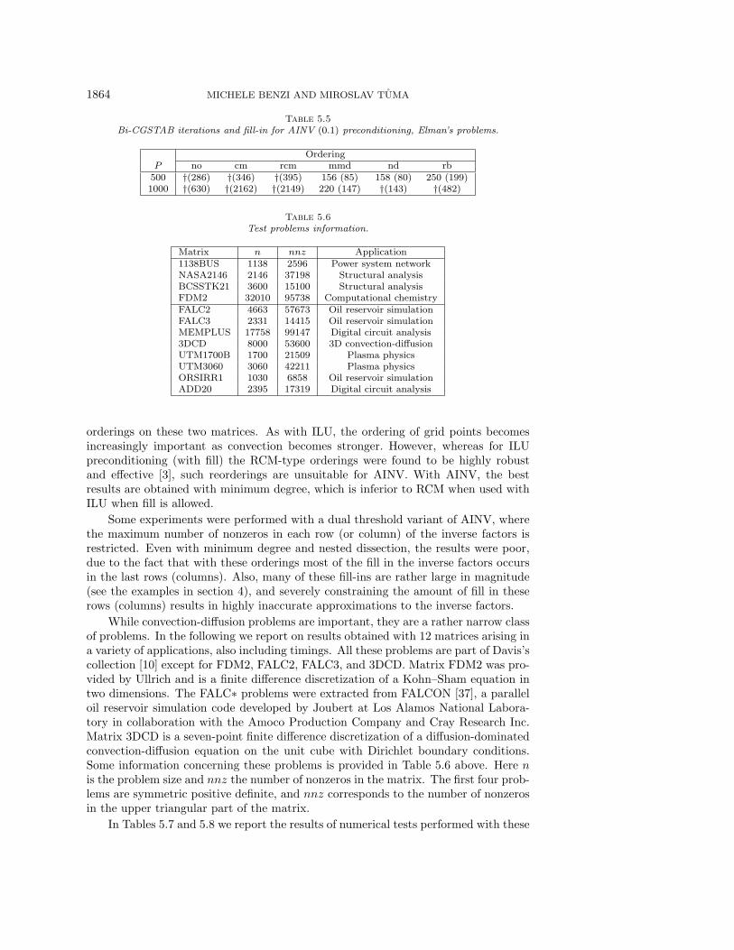
Table 5.6Test problems information.

Matrix n nnz Application1138BUS 1138 2596 Power system networkNASA2146 2146 37198 Structural analysisBCSSTK21 3600 15100 Structural analysisFDM2 32010 95738 Computational chemistryFALC2 4663 57673 Oil reservoir simulationFALC3 2331 14415 Oil reservoir simulationMEMPLUS 17758 99147 Digital circuit analysis3DCD 8000 53600 3D convection-diffusionUTM1700B 1700 21509 Plasma physicsUTM3060 3060 42211 Plasma physicsORSIRR1 1030 6858 Oil reservoir simulationADD20 2395 17319 Digital circuit analysis

orderings on these two matrices. As with ILU, the ordering of grid points becomesincreasingly important as convection becomes stronger. However, whereas for ILUpreconditioning (with fill) the RCM-type orderings were found to be highly robustand effective [3], such reorderings are unsuitable for AINV. With AINV, the bestresults are obtained with minimum degree, which is inferior to RCM when used withILU when fill is allowed.

Some experiments were performed with a dual threshold variant of AINV, wherethe maximum number of nonzeros in each row (or column) of the inverse factors isrestricted. Even with minimum degree and nested dissection, the results were poor,due to the fact that with these orderings most of the fill in the inverse factors occursin the last rows (columns). Also, many of these fill-ins are rather large in magnitude(see the examples in section 4), and severely constraining the amount of fill in theserows (columns) results in highly inaccurate approximations to the inverse factors.

While convection-diffusion problems are important, they are a rather narrow classof problems. In the following we report on results obtained with 12 matrices arising ina variety of applications, also including timings. All these problems are part of Davis’scollection [10] except for FDM2, FALC2, FALC3, and 3DCD. Matrix FDM2 was pro-vided by Ullrich and is a finite difference discretization of a Kohn–Sham equation intwo dimensions. The FALC∗ problems were extracted from FALCON [37], a paralleloil reservoir simulation code developed by Joubert at Los Alamos National Labora-tory in collaboration with the Amoco Production Company and Cray Research Inc.Matrix 3DCD is a seven-point finite difference discretization of a diffusion-dominatedconvection-diffusion equation on the unit cube with Dirichlet boundary conditions.Some information concerning these problems is provided in Table 5.6 above. Here nis the problem size and nnz the number of nonzeros in the matrix. The first four prob-lems are symmetric positive definite, and nnz corresponds to the number of nonzerosin the upper triangular part of the matrix.

In Tables 5.7 and 5.8 we report the results of numerical tests performed with these

ORDERINGS FOR FACTORIZED INVERSE PRECONDITIONERS 1865

Table 5.7Test results, symmetric positive definite problems.

Matrix original mmd gnd rcm mcl1138BUS 4464/0.063 6422/0.066 4520/0.061 8426/0.074 4092/0.066

82/0.107 57/0.088 69/0.091 46/0.085 79/0.099NASA2146 31956/0.454 23264/0.660 24825/0.510 35177/0.561 306051/16.45

335/5.358 249/3.446 323/4.511 430/6.916 – / –BCSSTK21 113104/0.915 15789/0.291 24229/0.305 31691/0.315 14669/0.260

–/– 220/1.656 2072/18.09 –/– 197/1.470FDM2 169127/1.716 132791/2.216 130839/1.967 166156/1.871 145779/1.826

257/32.70 217/24.05 210/23.75 237/29.74 196/22.11

Table 5.8Test results, nonsymmetric problems.

Matrix original mmd gnd rcm mclFALC2 107766/1.941 66885/1.449 93238/1.512 217415/2.036 72639/1.179

23/1.318 25/1.122 25/1.326 18/1.596 33/1.497FALC3 99384/0.743 58421/0.554 57281/0.547 136928/0.752 66717/0.583

29/0.900 21/0.360 26/0.442 20/0.906 28/0.575MEMPLUS 59547/2.389 44288/2.145 43914/2.222 55289/2.184 57298/2.371

189/17.75 17/1.923 264/22.89 17/1.838 27/2.7703DCD 102043/1.128 87288/1.554 88869/1.448 115477/1.255 82946/1.297

18/1.204 13/0.844 13/0.868 18/1.275 13/0.820UTM1700B 170899/2.511 65930/0.759 65631/0.837 145197/1.258 93301/2.572

903/46.66 232/4.502 641/11.74 324/14.46 659/18.80UTM3060 403616/5.014 118609/1.683 119956/1.751 378420/3.974 190163/6.342

976/117.7 115/5.526 124/5.999 377/42.16 234/15.11ORSIRR1 5351/0.124 4819/0.124 4764/0.123 5519/0.127 5049/0.121

32/0.078 33/0.081 35/0.084 29/0.072 34/0.084ADD20 7525/0.327 5912/0.269 5424/0.284 6892/0.260 6366/0.298

7/0.079 7/0.079 7/0.076 7/0.079 7/0.079

12 matrices and different orderings, performed on one processor of an SGI Origin 2000with R10000 processors. The results in Table 5.7 are relative to the SPD problems,for which conjugate gradient acceleration was used; in Table 5.8 we give the resultsfor the nonsymmetric problems, where Bi-CGSTAB was the accelerator of choice. Inall cases the stopping criterion was a reduction of the initial residual norm by at leasteight orders of magnitude. The drop tolerance in AINV was set to 0.1 for all problemsexcept for BCSSTK21, where we used 0.2, and for the FALC∗ matrices where a droptolerance equal to 0.01 was used. A “–” means no convergence. In the tables, “gnd”denotes a generalized nested dissection ordering [27] and “mcl” a greedy multicoloringheuristic [36]. For each matrix we provide the number of nonzeros in the approximateinverse factors with the time to compute the preconditioner (above) and the numberof iterations with the corresponding timing (below). Timings were measured by thedtime function. The codes were compiled by f77 with the -O3 option.

These results indicate that minimum degree is generally the best ordering, result-ing in most cases in small inverse fill and good convergence rates. Generalized nesteddissection is also good in general. The performance of RCM is not as poor as in theprevious set of experiments, although this ordering often results in high amounts ofinverse fill. Multicoloring is often better than the original ordering, and sometimes itoutperforms all the other orderings, but on the average is not as good as minimumdegree or nested dissection. As for the time to compute the preconditioner, it appearsthat fill-reducing orderings are not always effective at reducing timings. This could be

1866 MICHELE BENZI AND MIROSLAV TUMA

Table 5.9Results for FDM2, graph partitioning.

p PCG Its |Z|2 276 168,7864 276 168,6348 274 167,85016 275 164,38732 274 162,99964 274 157,032128 276 149,913256 276 144,085512 264 138,9541024 244 136,960

due to cache effects, considering that minimum degree and nested dissection are globalorderings that do not preserve data locality, which is often present with the originalordering or with RCM. It should also be mentioned that a good correlation betweeninverse fill and timings for the construction of AINV was observed in [7], possibly dueto the somewhat different implementation of AINV adopted in [7]. In any event, areduction in the amount of fill in the approximate inverse factors is important, par-ticularly for large problems. It is also worth mentioning that for symmetric problemspreordered with minimum degree, a small but worthwhile reduction in the time forthe set-up phase was achieved by applying equivalent postorderings to the computedinverse factors, using techniques described in [23], [29], [30]. In the interest of brevity,we do not report these results here.

Finally, we performed some experiments using the METIS graph partitioningpackage [24]. Graph partitioning affords a natural way to parallelize sparse matrixcomputations, and should be a valuable tool for parallelizing the AINV preconditioner,both in the set-up phase and in the iterative application of the approximate inverse.However, partitioning induces a reordering and we are interested in seeing the effecton the convergence rate. Because of the similarity with nested dissection, we expectthe performance to be satisfactory.

In Table 5.9 we show the results obtained for matrix FDM2 with the standardPMETIS executable code with default partitioning parameters. Here p denotes thenumber of subdomains, or graph partitions. In a parallel environment, p would beequal to the number of processors. It is interesting to see that the performance im-proves with the number of subdomains, both from the point of view of fill in theapproximate inverse factor Z and from the point of view of convergence rate, at leastup until p = 1024. These results suggest that efficient parallel implementations ofAINV are possible without sacrificing the quality of the preconditioner. For pre-liminary results obtained with a parallel implementation of AINV based on graphpartitioning, see [1].

6. Conclusions. We have presented theoretical results and numerical experi-ments aimed at assessing the effect of different sparse matrix orderings on the perfor-mance of the factorized approximate inverse preconditioner AINV. These experimentsappear to confirm the intuition that orderings which produce relatively sparse inversefactors, such as minimum degree and nested dissection, tend to perform better thanorderings (like RCM) that result in matrices with a narrow profile but dense inversefactors. This is especially true for difficult problems characterized by slow decay inthe inverse. This marks a significant difference between the behavior of factorized

ORDERINGS FOR FACTORIZED INVERSE PRECONDITIONERS 1867

sparse approximate inverse preconditioners and that of ILU-type techniques. A goodordering for AINV results not only in reduced storage needs for computing the approx-imate inverse factorization, but also in better convergence rates for the preconditionediteration. In several cases the preconditioned iteration failed with the original order-ing, but succeeded with an appropriate reordering, usually minimum degree. This isprobably due to the fact that with a good ordering, less entries in the inverse factorsare discarded, resulting in a more accurate approximation to the exact inverse.

An interesting problem, not considered here, is to look for reorderings which takeinto account the magnitude of the matrix entries and not just the sparsity struc-ture. Some weighted graph heuristics have been proposed in [7], and the results foranisotropic problems reported in [7] are encouraging. However, more work is neededin this direction.

Preliminary results using permutations induced by graph partitioning suggest thatparallelism can be achieved in the construction and application of the AINV precon-ditioner without compromising its effectiveness at reducing the number of iterations.Tests with a fully parallel implementation of AINV based on graph partitioning, re-ported in [1], have confirmed this observation.

Acknowledgments. During the preparation of this paper we have benefitedfrom insightful discussions with Robert Bridson, Tim Davis, John Gilbert, and GerardMeurant. We are also thankful to one of the referees for valuable comments andsuggestions.

REFERENCES

[1] M. Benzi, J. Marın, and M. Tuma, Parallel preconditioning with factorized sparse approx-imate inverses, in Proceedings of the Ninth SIAM Conference on Parallel Processing forScientific Computing, B. Hendrickson et al., eds., CD-ROM, SIAM, Philadelphia, PA, 1999.

[2] M. Benzi, C. D. Meyer, and M. Tuma, A sparse approximate inverse preconditioner for theconjugate gradient method, SIAM J. Sci. Comput., 17 (1996), pp. 1135–1149.

[3] M. Benzi, D. B. Szyld, and A. van Duin, Orderings for incomplete factorization precondi-tioning of nonsymmetric problems, SIAM J. Sci. Comput., 20 (1999), pp. 1652–1670.

[4] M. Benzi and M. Tuma, A sparse approximate inverse preconditioner for nonsymmetric linearsystems, SIAM J. Sci. Comput., 19 (1998), pp. 968–994.

[5] M. Benzi and M. Tuma, Numerical experiments with two approximate inverse preconditioners,BIT, 38 (1998), pp. 234–241.

[6] M. Benzi and M. Tuma, A comparative study of sparse approximate inverse preconditioners,Appl. Numer. Math., 30 (1999), pp. 305–340.

[7] R. Bridson and W.-P. Tang, Ordering, anisotropy and factored sparse approximate inverses,SIAM J. Sci. Comput., 21 (1999), pp. 867–882.

[8] T. Chan, W.-P. Tang, and W. Wan, Wavelet sparse approximate inverse preconditioners,BIT, 37 (1997), pp. 644-660.

[9] E. Chow and Y. Saad, Approximate inverse preconditioners via sparse-sparse iterations,SIAM J. Sci. Comput., 19 (1998), pp. 995–1023.

[10] T. Davis, University of Florida Sparse Matrix Collection, NA Digest, vol. 94, issue 42, October1994; also available online from http://www.cise.ufl.edu/∼davis/sparse/.

[11] S. Demko, W. F. Moss, and P. W. Smith, Decay rates for inverses of band matrices,Math. Comp., 43 (1984), pp. 491–499.

[12] I. S. Duff, A. M. Erisman, C. W. Gear, and J. K. Reid, Sparsity structure and Gaussianelimination, SIGNUM Newsletter, 23 (1988), pp. 2–9.

[13] I. S. Duff, A. M. Erisman, and J. K. Reid, Direct Methods for Sparse Matrices, ClarendonPress, Oxford, UK, 1986.

[14] I. S. Duff and G. A. Meurant, The effect of ordering on preconditioned conjugate gradients,BIT, 29 (1989), pp. 635–657.

[15] V. Eijkhout and B. Polman, Decay rates of inverses of banded M-matrices that are near toToeplitz matrices, Linear Algebra Appl., 109 (1988), pp. 247–277.

1868 MICHELE BENZI AND MIROSLAV TUMA

[16] H. C. Elman, Relaxed and stabilized incomplete factorizations for non-self-adjoint linearsystems, BIT, 29 (1989), pp. 890–915.

[17] M. R. Field, Improving the Performance of Factorised Sparse Approximate Inverse Precon-ditioner, Hitachi Dublin Laboratory Technical Report HDL-TR-98-199, Dublin, Ireland,1998.

[18] A. George and J. W. H. Liu, Computer Solution of Large Sparse Positive Definite Systems,Prentice–Hall, Englewood Cliffs, NJ, 1981.

[19] J. R. Gilbert, Predicting structure in sparse matrix computations, SIAM J. Matrix Anal.Appl., 15 (1994), pp. 62–79.

[20] J. R. Gilbert and J. W. H. Liu, Elimination structures for unsymmetric sparse LU factors,SIAM J. Matrix Anal. Appl., 14 (1993), pp. 334–352.

[21] G. H. Golub and C. F. Van Loan, Matrix Computations, 3rd ed., The Johns HopkinsUniversity Press, Baltimore and London, 1996.

[22] M. Grote and T. Huckle, Parallel preconditioning with sparse approximate inverses, SIAMJ. Sci. Comput., 18 (1997), pp. 838–853.

[23] H. Hafsteinsson, Parallel Sparse Cholesky Factorization, Ph.D. Thesis, Department of Com-puter Science, Cornell University, 1988.

[24] G. Karypis and V. Kumar, METIS: A Software Package for Partitioning UnstructuredGraphs, Partitioning Meshes, and Computing Fill-Reducing Orderings of Sparse Matrices(Version 3.0), University of Minnesota, Department of Computer Science and Army HPCResearch Center, Minneapolis, MN, 1997.

[25] L. Yu. Kolotilina and A. Yu. Yeremin, Factorized sparse approximate inverse precondi-tioning I: Theory, SIAM J. Matrix Anal. Appl., 14 (1993), pp. 45–58.

[26] J. G. Lewis, B. W. Peyton, and A. Pothen, A fast algorithm for reordering sparse matricesfor parallel factorization, SIAM J. Sci. Statist. Comput., 10 (1989), pp. 1156–1173.

[27] R. J. Lipton, D. J. Rose, and R. E. Tarjan, Generalized nested dissection, SIAM J. Nu-mer. Anal., 16 (1979), pp. 346–358.

[28] J. W. H. Liu, Modification of the minimum degree algorithm by multiple elimination, ACMTrans. Math. Software, 11 (1985), pp. 141–153.

[29] J. W. H. Liu, Equivalent sparse matrix reordering by elimination tree rotations, SIAMJ. Sci. Statist. Comput., 9 (1988), pp. 424–444.

[30] J. W. H. Liu, Reordering sparse matrices for parallel elimination, Parallel Comput., 11 (1989),pp. 73–91.

[31] F. Manne, Reducing the Height of an Elimination Tree through Local Reorderings, TechnicalReport CS-51-91, University of Bergen, Norway, 1991.

[32] G. Meurant, A review of the inverse of symmetric tridiagonal and block tridiagonal matrices,SIAM J. Matrix Anal. Appl., 13 (1992), pp. 707–728.

[33] G. Meurant, private communication, December 1997.[34] R. Nabben, Decay rates of the inverse of nonsymmetric tridiagonal and band matrices, SIAM

J. Matrix Anal. Appl., 20 (1999), pp. 820–837.[35] A. Pothen, The Complexity of Optimal Elimination Trees, Technical Report CS-88-13, Penn-

sylvania State University, University Park, PA, 1988.[36] Y. Saad, Iterative Methods for Sparse Linear Systems, PWS Publishing Co., Boston, 1996.[37] G. S. Shiralkar, R. E. Stephenson, W. D. Joubert, and B. van Bloemen-Waanders,

FALCON: A production quality distributed memory reservoir simulator, SPE Paper 37975,presented at the SPE Reservoir Simulation Symposium, Dallas, Texas, 8–11 June 1997.

[38] H. A. van der Vorst, Bi-CGSTAB: A fast and smoothly converging variant of Bi-CG forthe solution of non-symmetric linear systems, SIAM J. Sci. Statist. Comput., 12 (1992),pp. 631–644.