Discriminative learning of Bayesian networks via factorized conditional log-likelihood

Journal of Machine Learning Research 12 (2011) 2181-2210 Submitted 4/11; Published 7/11

Discriminative Learning of Bayesian Networksvia Factorized Conditional Log-Likelihood

Alexandra M. Carvalho ASMC@INESC-ID .PT

Department of Electrical EngineeringInstituto Superior Tecnico, Technical University of LisbonINESC-ID, R. Alves Redol 91000-029 Lisboa, Portugal

Teemu Roos [email protected] .FI

Department of Computer ScienceHelsinki Institute for Information TechnologyP.O. Box 68FI-00014 University of Helsinki, Finland

Arlindo L. Oliveira AML @INESC-ID .PT

Department of Computer Science and EngineeringInstituto Superior Tecnico, Technical University of LisbonINESC-ID, R. Alves Redol 91000-029 Lisboa, Portugal

Petri Myllym aki PETRI.MYLLYMAKI @CS.HELSINKI .FI

Department of Computer ScienceHelsinki Institute for Information TechnologyP.O. Box 68FI-00014 University of Helsinki, Finland

Editor: Russell Greiner

Abstract

We propose an efficient and parameter-free scoring criterion, the factorized conditionallog-likelihood (fCLL), for learning Bayesian network classifiers. The proposed score is an ap-proximation of the conditional log-likelihood criterion.The approximation is devised in order toguarantee decomposability over the network structure, as well as efficient estimation of the optimalparameters, achieving the same time and space complexity asthe traditional log-likelihood scoringcriterion. The resulting criterion has an information-theoretic interpretation based on interactioninformation, which exhibits its discriminative nature. Toevaluate the performance of the proposedcriterion, we present an empirical comparison with state-of-the-art classifiers. Results on a largesuite of benchmark data sets from the UCI repository show that fCLL-trained classifiers achieveat least as good accuracy as the best compared classifiers, using significantly less computationalresources.

Keywords: Bayesian networks, discriminative learning, conditionallog-likelihood, scoring crite-rion, classification, approximation

c©2011 Alexandra M. Carvalho, Teemu Roos, Arlindo L. Oliveira and Petri Myllymaki.

CARVALHO , ROOS, OLIVEIRA AND MYLLYM AKI

1. Introduction

Bayesian networks have been widely used for classification, see Friedman et al. (1997), Grossmanand Domingos (2004), Su and Zhang (2006) and references therein.However, they are often out-performed by much simpler methods (Domingos and Pazzani, 1997; Friedman et al., 1997). One ofthe likely causes for this appears to be the use of so calledgenerative learningmethods in choos-ing the Bayesian network structure as well as its parameters. In contrast togenerative learning,where the goal is to be able to describe (or generate) the entire data,discriminative learningfocuseson the capacity of a model to discriminate between different classes of instances. Unfortunately,discriminative learning of Bayesian network classifiers has turned out to be computationally muchmore challenging than generative learning. This led Friedman et al. (1997)to bring up the ques-tion: are there heuristic approaches that allow efficient discriminative learning of Bayesian networkclassifiers?

During the past years different discriminative approaches have beenproposed, which tend todecompose the problem into two tasks: (i) discriminative structure learning, and (ii) discriminativeparameter learning. Greiner and Zhou (2002) were among the first to work along these lines. Theyintroduced a discriminative parameter learning algorithm, called theExtended Logistic Regression(ELR) algorithm, that uses gradient descent to maximize theconditional log-likelihood(CLL) of theclass variable given the other variables. Their algorithm can be applied to an arbitrary Bayesian net-work structure. However, they only consideredgenerativestructure learning methods. Greiner andZhou (2002) demonstrated that their parameter learning method, although computationally more ex-pensive than the usual generative approach that only involves counting relative frequencies, leads toimproved parameter estimates. More recently, Su et al. (2008) have managed to significantly reducethe computational cost by proposing an alternative discriminative parameterlearning method, calledtheDiscriminative Frequency Estimate(DFE) algorithm, that exhibits nearly the same accuracy asthe ELR algorithm but is considerably more efficient.

Full structure and parameter learning based on the ELR algorithm is a burdensome task. Em-ploying the procedure of Greiner and Zhou (2002) would require a newgradient descent for eachcandidate network at each search step, turning the method computationally infeasible. Moreover,even in parameter learning, ELR is not guaranteed to find globally optimal CLLparameters. Rooset al. (2005) have showed that globally optimal solutions can be guaranteed only for network struc-tures that satisfy a certain graph-theoretic property, including for example, the naive Bayes andtree-augmented naive Bayes (TAN) structures (see Friedman et al., 1997) as special cases. Thework by Greiner and Zhou (2002) supports this result empirically by demonstrating that their ELRalgorithm is successful when combined with (generatively learned) TAN classifiers.

For discriminative structure learning, Kontkanen et al. (1998) and Grossman and Domingos(2004) propose to choose network structures by maximizing CLL while choosing parameters bymaximizing the parameter posterior or the (joint)log-likelihood(LL). TheBNC algorithmof Gross-man and Domingos (2004) is actually very similar to the hill-climbing algorithm of Heckerman et al.(1995), except that it uses CLL as the primary objective function. Grossman and Domingos (2004)also experiment with full structure and parameter optimization for CLL. However, they found thatfull optimization does not produce better results than those obtained by the much simpler approachwhere parameters are chosen by maximizing LL.

The contribution of this paper is to present two criteria similar to CLL, but with much bettercomputational properties. The criteria can be used for efficient learningof augmented naive Bayes

2182

FACTORIZED CONDITIONAL LOG-L IKELIHOOD

classifiers. We mostly focus on structure learning. Compared to the work ofGrossman and Domin-gos (2004), our structure learning criteria have the advantage of beingdecomposable, a propertythat enables the use of simple and very efficient search heuristics. For the sake of simplicity, weassume a binary valued class variable when deriving our results. However, the methods are directlyapplicable to multi-class classification, as demonstrated in the experimental part(Section 5).

Our first criterion is theapproximated conditional log-likelihood(aCLL). The proposed scoreis the minimum variance unbiased (MVU) approximation to CLL under a class of uniform priorson certain parameters of the joint distribution of the class variable and the other attributes. Weshow that for most parameter values, the approximation error is very small. However, the aCLLcriterion still has two unfavorable properties. First, the parameters that maximize aCLL are hard toobtain, which poses problems at the parameter learning phase, similar to thoseposed by using CLLdirectly. Second, the criterion is not well-behaved in the sense that it sometimes diverges when theparameters approach the usual relative frequency estimates (maximizing LL).

In order to solve these two shortcomings, we devise a second approximation, the factorizedconditional log-likelihood(fCLL). The fCLL approximation is uniformly bounded, and moreover,it is maximized by the easily obtainable relative frequency parameter estimates. ThefCLL criterionallows a neat interpretation as a sum of LL and another term involving theinteraction informationbetween a node, its parents, and the class variable; see Pearl (1988),Cover and Thomas (2006),Bilmes (2000) and Pernkopf and Bilmes (2005).

To gauge the performance of the proposed criteria in classification tasks,we compare themwith several popular classifiers, namely,tree augmented naive Bayes(TAN), greedy hill-climbing(GHC), C4.5,k-nearest neighbor(k-NN), support vector machine(SVM) and logistic regression(LogR). On a large suite of benchmark data sets from the UCI repository,fCLL-trained classifiersoutperform, with a statistically significant margin, their generatively-trained counterparts, as wellas C4.5,k-NN and LogR classifiers. Moreover,fCLL-optimal classifiers are comparable with ELRinduced ones, as well as SVMs (with linear, polynomial, and radial basis function kernels). Theadvantage offCLL with respect to these latter classifiers is that it is computationally as efficient asthe LL scoring criterion, and considerably more efficient than ELR and SVMs.

The paper is organized as follows. In Section 2 we review some basic concepts of Bayesian net-works and introduce our notation. In Section 3 we discuss generative and discriminative learning ofBayesian network classifiers. In Section 4 we present our scoring criteria, followed by experimentalresults in Section 5. Finally, we draw some conclusions and discuss future work in Section 6. Theproofs of the results stated throughout this paper are given in the Appendix.

2. Bayesian Networks

In this section we introduce some notation, while recalling relevant concepts and results concerningdiscrete Bayesian networks.

Let X be adiscrete random variabletaking values in a countable setX ⊂R. In all what follows,the domainX is finite. We denote ann-dimensionalrandom vectorby X = (X1, . . . ,Xn) where eachcomponentXi is a random variable overXi . For each variableXi , we denote the elements ofXi byxi1, . . . ,xir i wherer i is the number of valuesXi can take. The probability thatX takes valuex isdenoted byP(x), conditional probabilitiesP(x | z) being defined correspondingly.

A Bayesian network(BN) is defined by a pairB= (G,Θ), whereG refers to the graph structure,andΘ are the parameters. The structureG= (V,E) is adirected acyclic graph(DAG) with vertices

2183

CARVALHO , ROOS, OLIVEIRA AND MYLLYM AKI

(nodes)V, each corresponding to one of the random variablesXi , and edgesE representing directdependencies between the variables. The (possibly empty) set of nodesfrom which there is anedge to nodeXi is called the set of theparentsof Xi , and denoted byΠXi . For each nodeXi , wedenote the number of possibleparent configurations(vectors of the parents’ values) byqi , the actualparent configurations being ordered (arbitrarily) and denoted bywi1, . . . ,wiqi . Theparameters, Θ ={θi jk}i∈{1,...,n}, j∈{1,...,qi},k∈{1,...,r i}, determine thelocal distributionsin the network via

PB(Xi = xik |ΠXi = wi j ) = θi jk .

The local distributions define a unique joint probability distribution overX given by

PB(X1, . . . ,Xn) =n

∏i=1

PB(Xi |ΠXi ).

The conditional independence properties pertaining to the joint distribution are essentially deter-mined by the network structure. Specifically,Xi is conditionally independent of its non-descendantsgiven its parentsΠXi in G (Pearl, 1988).

Learning unrestricted Bayesian networks from data under typical scoring criteria is NP-hard(Chickering et al., 2004). This result has led the Bayesian network community to search for thelargest subclass of network structures for which there is an efficient learning algorithm. First at-tempts confined the network to tree structures and used Edmonds (1967) and Chow and Liu (1968)optimal branching algorithms. More general classes of Bayesian networks have eluded efforts todevelop efficient learning algorithms. Indeed, Chickering (1996) showed that learning the struc-ture of a Bayesian network is NP-hard even for networks constrained tohave in-degree at mosttwo. Later, Dasgupta (1999) showed that even learning an optimalpolytree(a DAG in which thereare not two different paths from one node to another) with maximum in-degree two is NP-hard.Moreover, Meek (2001) showed that identifying the bestpath structure, that is, a total order overthe nodes, is hard. Due to these hardness results exact polynomial-time algorithms for learningBayesian networks have been restricted to tree structures.

Consequently, the standard methodology for addressing the problem of learning Bayesian net-works has become heuristic score-based learning where ascoring criterionφ is considered in or-der to quantify the capability of a Bayesian network to explain the observed data. Given dataD = {y1, . . . ,yN} and a scoring criterionφ, the task is to find a Bayesian networkB that maxi-mizes the scoreφ(B,D). Many search algorithms have been proposed, varying both in terms of theformulation of the search space (network structures, equivalence classes of network structures andorderings over the network variables), and in the algorithm to search the space (greedy hill-climbing,simulated annealing, genetic algorithms, tabu search, etc). The most common scoring criteria arereviewed in Carvalho (2009) and Yang and Chang (2002). We refer the interested reader to newlydeveloped scoring criteria to the works of de Campos (2006) and Silanderet al. (2010).

Score-based learning algorithms can be extremely efficient if the employed scoring criterion isdecomposable. A scoring criterionφ is said to bedecomposableif the score can be expressed as asum of local scores that depends only on each node and its parents, that is, in the form

φ(B,D) =n

∑i=1

φi(ΠXi ,D).

2184

FACTORIZED CONDITIONAL LOG-L IKELIHOOD

One of the most common criteria is thelog-likelihood(LL), see Heckerman et al. (1995):

LL(B | D) =N

∑t=1

logPB(y1t , . . . ,y

nt ) =

n

∑i=1

qi

∑j=1

r i

∑k=1

Ni jk logθi jk ,

which is clearly decomposable.Themaximum likelihood(ML) parameters that maximize LL are easily obtained as theobserved

frequency estimates(OFE) given by

θi jk =Ni jk

Ni j, (1)

whereNi jk denotes the number of instances inD whereXi = xik andΠXi = wi j , andNi j = ∑r ik=1Ni jk .

Plugging these estimates back into the LL criterion yields

LL(G | D) =n

∑i=1

qi

∑j=1

r i

∑k=1

Ni jk log

(Ni jk

Ni j

).

The notation withG as the argument instead ofB= (G,Θ) emphasizes that once the use of the OFEparameters is decided upon, the criterion is a function of the network structure,G, only.

The LL scoring criterion tends to favor complex network structures with many edges sinceadding an edge never decreases the likelihood. This phenomenon leads tooverfitting which isusually avoided by adding a complexity penalty to the log-likelihood or by restricting the networkstructure.

3. Bayesian Network Classifiers

A Bayesian network classifieris a Bayesian network overX = (X1, . . . ,Xn,C), whereC is a classvariable, and the goal is to classify instances(X1, . . . ,Xn) to different classes. The variablesX1, . . . ,Xn

are calledattributes, or features. For the sake of computational efficiency, it is common to restrictthe network structure. We focus onaugmented naive Bayes classifiers, that is, Bayesian networkclassifiers where the class variable has no parents,ΠC = /0, and all attributes have at least the classvariable as a parent,C∈ΠXi for all Xi .

For convenience, we introduce a few additional notations that apply to augmented naive Bayesmodels. Let the class variableC range overs distinct values, and denote them byz1, . . . ,zs. Recallthat the parents ofXi are denoted byΠXi . The parents ofXi without the class variable are denotedby Π∗Xi

= ΠXi \ {C}. We denote the number of possible configurations of the parent setΠ∗Xiby

q∗i ; hence,q∗i = ∏Xj∈Π∗Xir j . The j ’th configuration ofΠ∗Xi

is represented byw∗i j , with 1≤ j ≤ q∗i .Similarly to the general case, local distributions are determined by the corresponding parameters

P(C= zc) = θc,

P(Xi = xik |Π∗Xi= w∗i j ,C= zc) = θi jck.

We denote byNi jck the number of instances in the dataD whereXi = xik, Π∗Xi= w∗i j andC= zc.

Moreover, the following short-hand notations will become useful:

Ni j∗k =s

∑c=1

Ni jck, Ni j∗ =r i

∑k=1

s

∑c=1

Ni jck,

Ni jc =r i

∑k=1

Ni jck, Nc =1n

n

∑i=1

q∗i

∑j=1

r i

∑k=1

Ni jck.

2185

CARVALHO , ROOS, OLIVEIRA AND MYLLYM AKI

Finally, we recall that the total number of instances in the dataD is N.The ML estimates (1) become now

θc =Nc

N, and θi jck =

Ni jck

Ni jc, (2)

which can again be plugged into the LL criterion:

LL(G | D) =N

∑t=1

logPB(y1t , . . . ,y

nt ,ct)

=s

∑c=1

(Nc log

(Nc

N

)+

n

∑i=1

qi

∑j=1

r i

∑k=1

Ni jck log

(Ni jck

Ni jc

)). (3)

As mentioned in the introduction, if the goal is to discriminate between instances belongingto different classes, it is more natural to consider theconditional log-likelihood(CLL), that is, theprobability of the class variable given the attributes, as a score:

CLL(B | D) =N

∑t=1

logPB(ct | y1t , . . . ,y

nt ).

Friedman et al. (1997) noticed that the log-likelihood can be rewritten as

LL(B | D) = CLL(B | D)+N

∑t=1

logPB(y1t , . . . ,y

nt ). (4)

Interestingly, the objective of generative learning is precisely to maximize thewhole sum, whereasthe goal of discriminative learning consists on maximizing only the first term in (4). Friedman et al.(1997) attributed the underperformance of learning methods based on LLto the term CLL(B | D)being potentially much smaller than the second term in Equation (4). Unfortunately, CLL doesnot decompose over the network structure, which seriously hinders structure learning, see Bilmes(2000); Grossman and Domingos (2004). Furthermore, there is no closed-form formula for optimalparameter estimates maximizing CLL, and computationally more expensive techniques such as ELRare required (Greiner and Zhou, 2002; Su et al., 2008).

4. Factorized Conditional Log-Likelihood Scoring Criterion

The above shortcomings of earlier discriminative approaches to learning Bayesian network clas-sifiers, and the CLL criterion in particular, make it natural to explore good approximations to theCLL that are more amenable to efficient optimization. More specifically, we nowset out to constructapproximations that aredecomposable, as discussed in Section 2.

4.1 Developing a New Scoring Criterion

For simplicity, assume that the class variable is binary,C = {0,1}. For the binary case the condi-tional probability of the class variable can then be written as

PB(ct | y1t , . . . ,y

nt ) =

PB(y1t , . . . ,y

nt ,ct)

PB(y1t , . . . ,y

nt ,ct)+PB(y1

t , . . . ,ynt ,1−ct)

. (5)

2186

FACTORIZED CONDITIONAL LOG-L IKELIHOOD

For convenience, we denote the two terms in the denominator as

Ut = PB(y1t , . . . ,y

nt ,ct) and

Vt = PB(y1t , . . . ,y

nt ,1−ct), (6)

so that Equation (5) becomes simply

PB(ct | y1t , . . . ,y

nt ) =

Ut

Ut +Vt.

We stress that bothUt andVt depend onB, but for the sake of readability we omitB in the notation.Observe that while(y1

t , . . . ,ynt ,ct) is thet ’th sample in the data setD, the vector(y1

t , . . . ,ynt ,1−ct),

which we call thedual sampleof (y1t , . . . ,y

nt ,ct), may or may not occur inD.

The log-likelihood (LL), and the conditional log-likelihood (CLL) now take the form

LL(B | D) =N

∑t=1

logUt , and

CLL(B | D) =N

∑t=1

logUt − log(Ut +Vt).

Recall that our goal is to derive a decomposable scoring criterion. Unfortunately, even though logUt

decomposes, log(Ut +Vt) does not.Now, let us consider approximating the log-ratio

f (Ut ,Vt) = log

(Ut

Ut +Vt

),

by functions of the formf (Ut ,Vt) = α logUt +β logVt + γ,

whereα, β, andγ are real numbers to be chosen so as to minimize the approximation error. Sincetheaccuracy of the approximation obviously depends on the values ofUt andVt as well as the constantsα, β, andγ, we need to make some assumptions aboutUt andVt in order to determine suitable valuesof α, β andγ. We explicate one possible set of assumptions, which will be seen to lead to a goodapproximation for a very wide range ofUt andVt . We emphasize that the role of the assumptions isto aid in arriving at good choices of the constantsα, β, andγ, after which we can dispense with theassumptions—they need not, in particular, hold true exactly.

Start by noticing thatRt = 1− (Ut +Vt) is the probability of observing neither thet ’th sam-ple nor its dual, and hence, the triplet(Ut ,Vt ,Rt) are the parameters of a trinomial distribution. Weassume, for the time being, that no knowledge about the values of the parameters(Ut ,Vt ,Rt) is avail-able. Therefore, it is natural to assume that(Ut ,Vt ,Rt) follows the uniform Dirichlet distribution,Dirichlet(1,1,1), which implies that

(Ut ,Vt)∼ Uniform(∆2), (7)

where∆2 = {(x,y) : x+y≤ 1 andx,y≥ 0} is the 2-simplex set. However, with a brief reflection onthe matter, we can see that such an assumption is actually rather unrealistic. Firstly, by inspectingthe total number of possible observed samples, we expect,Rt to be relatively large (close to 1).

2187

CARVALHO , ROOS, OLIVEIRA AND MYLLYM AKI

In fact, Ut andVt are expected to become exponentially small as the number of attributes grows.Therefore, it is reasonable to assume that

Ut ,Vt ≤ p<12< Rt

for some 0< p< 12. Combining this constraint with the uniformity assumption, Equation (7), yields

the following assumption, which we will use as a basis for our further analysis.

Assumption 1 There exists a small positivep< 12 such that

(Ut ,Vt)∼ Uniform(∆2)|Ut ,Vt≤p = Uniform([0, p]× [0, p]).

Assumption 1 implies thatUt andVt are uniform i.i.d. random variables over[0, p] for some(possibly unknown) positive real numberp< 1

2. (See Appendix B for an alternative justification forAssumption 1.) As we show below, we do not need to know the actual value ofp. Consequently,the envisaged approximation will be robust to the choice ofp.

We obtain the best fitting approximationf by the least squares method.

Theorem 1 Under Assumption 1, the values ofα, β andγ that minimize themean square error(MSE) of f w.r.t. f are given by

α =π2+6

24, (8)

β =π2−18

24, and (9)

γ =π2

12ln2−

(2+

(π2−6) logp12

), (10)

where log is the binary logarithm and ln is the natural logarithm.

We show that the mean difference betweenf and f is zero for all values ofp, that is, f isunbiased.1 Moreover, we show thatf is the approximation with the lowest variance among unbiasedones.

Theorem 2 The approximationf with α, β, γ defined as in Theorem 1 is theminimum varianceunbiased(MVU) approximation off .

Next, we derive the standard error of the approximationf in the square[0, p]× [0, p], which,curiously, does not depend onp. To this end, consider

µ= E[ f (Ut ,Vt)] =1

2ln(2)−2

which is a negative value; as it should sincef ranges over(−∞,0].

1. Herein we apply the nomenclature of estimation theory in the context of approximation. Thus, an approximationis unbiasedif E[ f (Ut ,Vt)− f (Ut ,Vt)] = 0 for all p. Moreover, an approximation is(uniformly) minimum varianceunbiasedif the valueE[( f (Ut ,Vt)− f (Ut ,Vt))

2] is the lowest for all unbiased approximations and values ofp.

2188

FACTORIZED CONDITIONAL LOG-L IKELIHOOD

Theorem 3 The approximationf with α, β, andγ defined as in Theorem 1 hasstandard errorgivenby

σ =

√36+36π2−π4

288ln2(2)−2≈ 0.352

andrelative standard errorσ/|µ| ≈ 0.275.

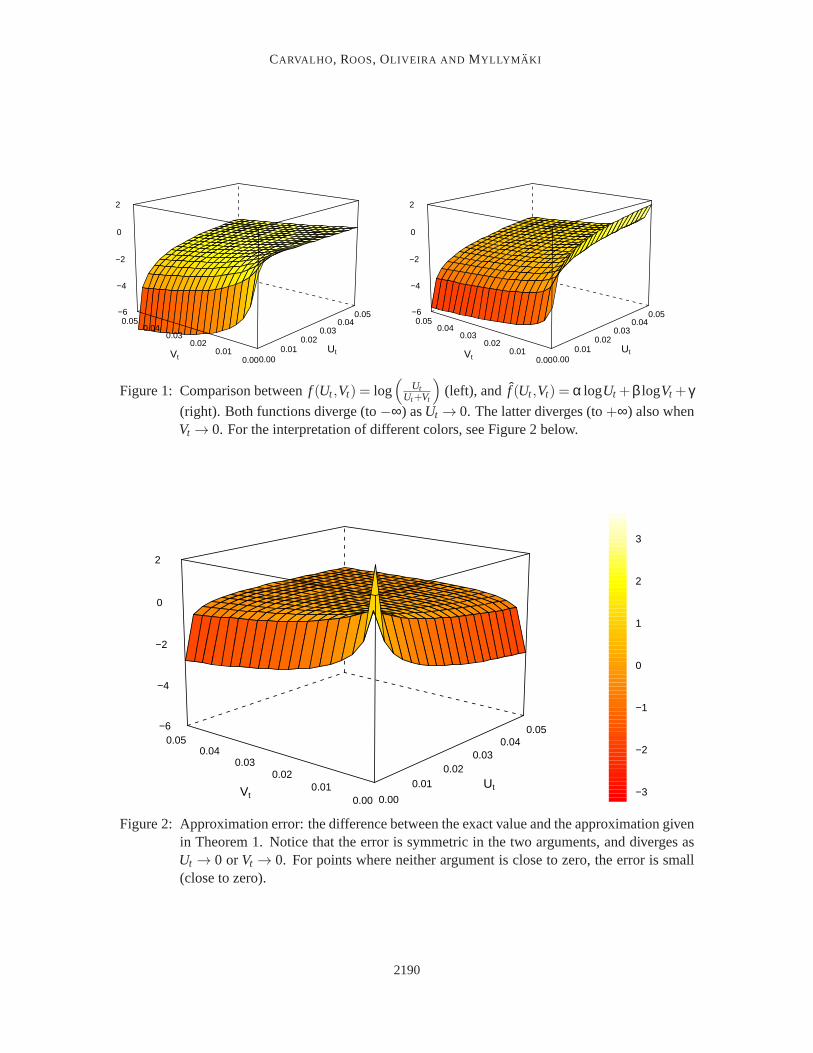
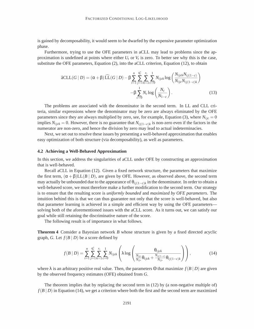
Figure 1 illustrates the functionf as well as its approximationf for (Ut ,Vt) ∈ [0, p]× [0, p] withp = 0.05. The approximation error,f − f is shown in Figure 2. While the properties establishedin Theorems 1–3 are useful, we find it even more important that, as seen in Figure 2, the error isclose to zero except when eitherUt or Vt approaches zero. Moreover, we point out that the choiceof p= 0.05 used in the figure is not important: having chosen another value would have producedidentical graphs except in the scale of theUt andVt . In particular, the scale and numerical values onthe vertical axis (i.e., in Figure 2, the error) would have been precisely thesame.

Using the approximation in Theorem 1 to approximate CLL yields

CLL(B | D) ≈N

∑t=1

α logUt +β logVt + γ

=N

∑t=1

(α+β) logUt −β log

(Ut

Vt

)+ γ

= (α+β)LL(B | D)−βN

∑t=1

log

(Ut

Vt

)+Nγ, (11)

where constantsα, β andγ are given by Equations (8), (9) and (10), respectively. Since we want tomaximize CLL(B | D), we can drop the constantNγ in the approximation, as maxima are invariantunder monotone transformations, and so we can just maximize the following formula, which wecall theapproximate conditional log-likelihood(aCLL):

aCLL(B | D) = (α+β)LL(B | D)−βN

∑t=1

log

(Ut

Vt

)

= (α+β)LL(B | D)−βn

∑i=1

q∗i

∑j=1

r i

∑k=1

1

∑c=0

Ni jck log

(θi jck

θi j (1−c)k

)

−β1

∑c=0

Nc log

(θc

θ(1−c)

). (12)

The fact thatNγ can be removed from the maximization in (11) is most fortunate, as we eliminatethe dependency onp. An immediate consequence of this fact is that we do not need to know theactual value ofp in order to employ the criterion.

We are now in the position of having constructed adecomposableapproximation of the condi-tional log-likelihood score that was shown to be very accurate for a wide range of parametersUt

andVt . Due to the dependency of these parameters onΘ, that is, the parameters of the BayesiannetworkB (recall Equation (6)), the score still requires that a suitable set of parameters is chosen.Finding the parameters maximizing the approximation is, however, difficult; apparently as difficultas finding parameters maximizing the CLL directly. Therefore, whatever computational advantage

2189

CARVALHO , ROOS, OLIVEIRA AND MYLLYM AKI

0.000.01

0.020.03

0.040.05

0.000.01

0.020.03

0.040.05

−6

−4

−2

0

2

UtVt 0.000.01

0.020.03

0.040.05

0.000.01

0.020.03

0.040.05

−6

−4

−2

0

2

UtVt

Figure 1: Comparison betweenf (Ut ,Vt) = log(

UtUt+Vt

)(left), and f (Ut ,Vt) = α logUt +β logVt + γ

(right). Both functions diverge (to−∞) asUt → 0. The latter diverges (to+∞) also whenVt → 0. For the interpretation of different colors, see Figure 2 below.

0.00

0.010.02

0.030.04

0.05

0.000.01

0.020.03

0.040.05

−6

−4

−2

0

2

UtVt −3

−2

−1

0

1

2

3

Figure 2: Approximation error: the difference between the exact value and the approximation givenin Theorem 1. Notice that the error is symmetric in the two arguments, and diverges asUt → 0 orVt → 0. For points where neither argument is close to zero, the error is small(close to zero).

2190

FACTORIZED CONDITIONAL LOG-L IKELIHOOD

is gained by decomposability, it would seem to be dwarfed by the expensiveparameter optimizationphase.

Furthermore, trying to use the OFE parameters in aCLL may lead to problems since the ap-proximation is undefined at points where eitherUt or Vt is zero. To better see why this is the case,substitute the OFE parameters, Equation (2), into the aCLL criterion, Equation(12), to obtain

aCLL(G | D) = (α+β) LL(G | D)−βn

∑i=1

q∗i

∑j=1

r i

∑k=1

1

∑c=0

Ni jck log

(Ni jckNi j (1−c)

Ni jcNi j (1−c)k

)

−β1

∑c=0

Nc log

(Nc

N1−c

). (13)

The problems are associated with the denominator in the second term. In LL andCLL cri-teria, similar expressions where the denominator may be zero are always eliminated by the OFEparameters since they are always multiplied by zero, see, for example, Equation (3), whereNi jc = 0impliesNi jck = 0. However, there is no guarantee thatNi j (1−c)k is non-zero even if the factors in thenumerator are non-zero, and hence the division by zero may lead to actual indeterminacies.

Next, we set out to resolve these issues by presenting a well-behaved approximation that enableseasy optimization of both structure (via decomposability), as well as parameters.

4.2 Achieving a Well-Behaved Approximation

In this section, we address the singularities of aCLL under OFE by constructing an approximationthat is well-behaved.

Recall aCLL in Equation (12). Given a fixed network structure, the parameters that maximizethe first term,(α+β)LL(B | D), are given by OFE. However, as observed above, the second termmay actually be unbounded due to the appearance ofθi j (1−c)k in the denominator. In order to obtain awell-behaved score, we must therefore make a further modification to the second term. Our strategyis to ensure that the resulting score isuniformly boundedandmaximized by OFE parameters. Theintuition behind this is that we can thus guarantee not only that the score is well-behaved, but alsothat parameter learning is achieved in a simple and efficient way by using the OFE parameters—solving both of the aforementioned issues with the aCLL score. As it turns out, we can satisfy ourgoal while still retaining the discriminative nature of the score.

The following result is of importance in what follows.

Theorem 4 Consider a Bayesian networkB whose structure is given by a fixed directed acyclicgraph,G. Let f (B | D) be a score defined by

f (B | D) =n

∑i=1

q∗i

∑j=1

r i

∑k=1

1

∑c=0

Ni jck

λ log

θi jck

Ni jc

Ni j∗θi jck +

Ni j (1−c)

Ni j∗θi j (1−c)k

, (14)

whereλ is an arbitrary positive real value. Then, the parametersΘ that maximizef (B |D) are givenby the observed frequency estimates (OFE) obtained fromG.

The theorem implies that by replacing the second term in (12) by (a non-negative multiple of)f (B |D) in Equation (14), we get a criterion where both the first and the second term are maximized

2191

CARVALHO , ROOS, OLIVEIRA AND MYLLYM AKI

by the OFE parameters. We will now proceed to determine a suitable value for the parameterλappearing in Equation (14).

To clarify the analysis, we introduce the following short-hand notations:

A1 = Ni jcθi jck, A2 = Ni jc ,

B1 = Ni j (1−c)θi j (1−c)k, B2 = Ni j (1−c).(15)

With simple algebra, we can rewrite the logarithm in the second term of Equation (12) using theabove notations as

log

(Ni jcθi jck

Ni j (1−c)θi j (1−c)k

)− log

(Ni jc

Ni j (1−c)

)= log

(A1

B1

)− log

(A2

B2

). (16)

Similarly, the logarithm in (14) becomes

λ log

(Ni jcθi jck

Ni jcθi jck +Ni j (1−c)θi j (1−c)k

)+ρ−λ log

(Ni jc

Ni jc +Ni j (1−c)

)−ρ

= λ log

(A1

A1+B1

)+ρ−λ log

(A2

A2+B2

)−ρ, (17)

where we usedNi j∗ = Ni jc +Ni j (1−c); we have introduced the constantρ that was added and sub-tracted without changing the value of the expression for a reason that willbecome clear shortly. Bycomparing Equations (16) and (17), it can be seen that the latter is obtainedfrom the former byreplacing expressions of the form log(A

B) by expressions of the formλ log( AA+B)+ρ.

We can simplify the two-variable approximation to a single variable one by takingW = AA+B. In

this case we have thatAB = W

1−W , and so we propose to apply once again the least squares method toapproximate the function

g(W) = log

(W

1−W

)

byg(W) = λ logW+ρ.

The role of the constantρ is simply to translate the approximate function to better match the targetg(W).

As in the previous approximation, here too it is necessary to make assumptionsabout the valuesof A andB (and thusW), in order to find suitable values for the parametersλ andρ. Again, we stressthat the sole purpose of the assumption is to guide in the choice of the parameters.

As bothA1, A2, B1, andB2 in Equation (15) are all non-negative, the ratioWi =Ai

Ai+Biis al-

ways between zero and one, for bothi ∈ {1,2}, and hence it is natural to make the straightforwardassumption thatW1 andW2 are uniformly distributed along the unit interval. This gives us thefollowing assumption.

Assumption 2 We assume that

Ni jcθi jck

Ni jcθi jck +Ni j (1−c)θi j (1−c)k∼ Uniform(0,1), and

Ni jc

Ni jc +Ni j (1−c)∼ Uniform(0,1).

2192

FACTORIZED CONDITIONAL LOG-L IKELIHOOD

g(w)

g`

(w)

0.2 0.4 0.6 0.8 1.0w

-4

-3

-2

-1

0

1

2

3

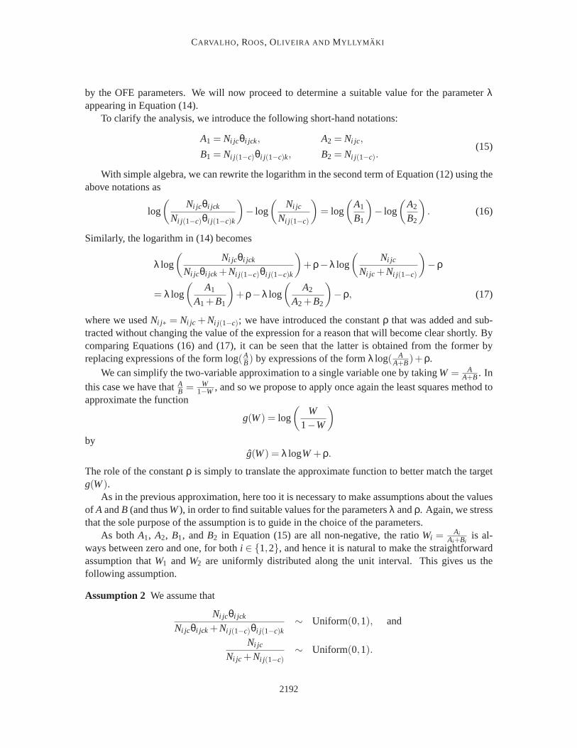
Figure 3: Plot ofg(w) = log(

w1−w

)andg(w) = λ logw+ρ.

Herein, it is worthwhile noticing that although the previous assumption was meant to hold forgeneral parameters, in practice, we know in this case that OFE will be used. Hence, Assumption 2reduces to

Ni jck

Ni j∗k∼ Uniform(0,1), and

Ni jc

Ni j∗∼ Uniform(0,1).

Under this assumption, the mean squared error of the approximation can be minimized analyti-cally, yielding the following solution.

Theorem 5 Under Assumption 2, the values ofλ andρ that minimize the mean square error (MSE)of g w.r.t. g are given by

λ =π2

6, and (18)

ρ =π2

6ln2. (19)

Theorem 6 The approximation ˆg with λ andρ defined as in Theorem 5 is the minimum varianceunbiased (MVU) approximation ofg.

In order to get an idea of the accuracy of the approximation ˆg, consider the graph of log(

w1−w

)

andλ logw+ρ in Figure 3. It may appear problematic that the approximation gets worse asw tendsto one. However this is actually unavoidable since that is precisely whereaCLL diverges, and ourgoal is to obtain a criterion that is uniformly bounded.

To wrap up, we first rewrite the logarithm of the second term in Equation (12) using for-mula (16), and then apply the above approximation to both terms to get

log

(θi jck

θi j (1−c)k

)≈ λ log

(Ni jcθi jck

Ni jcθi jck +Ni j (1−c)θi j (1−c)k

)+ρ−λ log

(Ni jc

Ni j∗

)−ρ, (20)

whereρ cancels out. A similar analysis can be applied to rewrite the logarithm of the third term inEquation (12) leading to

log

(θc

θ(1−c)

)= log

(θc

1−θc

)≈ λ logθc+ρ. (21)

2193

CARVALHO , ROOS, OLIVEIRA AND MYLLYM AKI

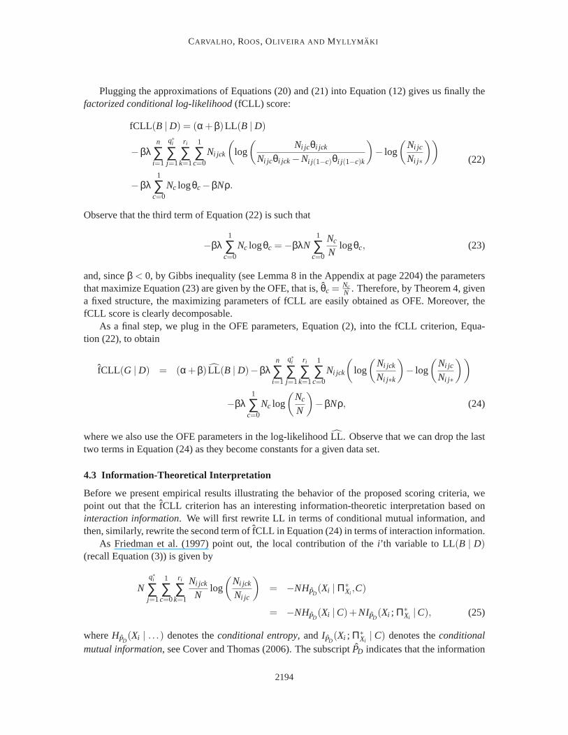
Plugging the approximations of Equations (20) and (21) into Equation (12) gives us finally thefactorized conditional log-likelihood(fCLL) score:

fCLL(B | D) = (α+β)LL(B | D)

−βλn

∑i=1

q∗i

∑j=1

r i

∑k=1

1

∑c=0

Ni jck

(log

(Ni jcθi jck

Ni jcθi jck−Ni j (1−c)θi j (1−c)k

)− log

(Ni jc

Ni j∗

))

−βλ1

∑c=0

Nc logθc−βNρ.

(22)

Observe that the third term of Equation (22) is such that

−βλ1

∑c=0

Nc logθc =−βλN1

∑c=0

Nc

Nlogθc, (23)

and, sinceβ < 0, by Gibbs inequality (see Lemma 8 in the Appendix at page 2204) the parametersthat maximize Equation (23) are given by the OFE, that is,θc =

NcN . Therefore, by Theorem 4, given

a fixed structure, the maximizing parameters of fCLL are easily obtained as OFE. Moreover, thefCLL score is clearly decomposable.

As a final step, we plug in the OFE parameters, Equation (2), into the fCLL criterion, Equa-tion (22), to obtain

fCLL(G | D) = (α+β) LL(B | D)−βλn

∑i=1

q∗i

∑j=1

r i

∑k=1

1

∑c=0

Ni jck

(log

(Ni jck

Ni j∗k

)− log

(Ni jc

Ni j∗

))

−βλ1

∑c=0

Nc log

(Nc

N

)−βNρ, (24)

where we also use the OFE parameters in the log-likelihoodLL. Observe that we can drop the lasttwo terms in Equation (24) as they become constants for a given data set.

4.3 Information-Theoretical Interpretation

Before we present empirical results illustrating the behavior of the proposed scoring criteria, wepoint out that thefCLL criterion has an interesting information-theoretic interpretation based oninteraction information. We will first rewrite LL in terms of conditional mutual information, andthen, similarly, rewrite the second term offCLL in Equation (24) in terms of interaction information.

As Friedman et al. (1997) point out, the local contribution of thei’th variable to LL(B | D)(recall Equation (3)) is given by

Nq∗i

∑j=1

1

∑c=0

r i

∑k=1

Ni jck

Nlog

(Ni jck

Ni jc

)= −NHPD

(Xi |Π∗Xi,C)

= −NHPD(Xi |C)+NIPD

(Xi ; Π∗Xi|C), (25)

whereHPD(Xi | . . .) denotes theconditional entropy, andIPD

(Xi ; Π∗Xi| C) denotes theconditional

mutual information, see Cover and Thomas (2006). The subscriptPD indicates that the information

2194

FACTORIZED CONDITIONAL LOG-L IKELIHOOD

theoretic quantities are evaluated under the joint distributionPD of (~X,C) induced by the OFEparameters.

Since the first term on the right-hand side of (25) does not depend onΠ∗Xi, finding the parents

of Xi that maximize LL(B |D) is equivalent to choosing the parents that maximize the second term,NIPD

(Xi ; Π∗Xi|C), which measures the information thatΠ∗Xi

provides aboutXi when the value ofCis known.

Let us now turn to the second term of thefCLL score in Equation (24). The contribution of thei’th variable in it can also be expressed in information theoretic terms as follows:

−βλN(HPD

(C | Xi ,Π∗Xi)−HPD

(C |Π∗Xi))= βλNIPD

(C; Xi |Π∗Xi)

= βλN(IPD

(C; Xi ; Π∗Xi)+ IPD

(C; Xi))),

(26)

whereIPD(C; XI ; Π∗Xi

) denotes theinteraction information(McGill, 1954), or the“co-information”(Bell, 2003); for a review on the history and use of interaction information inmachine learning andstatistics, see Jakulin (2005).

SinceIPD(Xi ; C) on the last line of Equation (26) does not depend onΠ∗Xi

, finding the parents ofXi that maximize the sum amounts to maximizing the interaction information. This is intuitive, sincethe interaction information measures the increase—or the decrease, as it can also be negative—ofthe mutual information betweenXi andC when the parent setΠ∗Xi

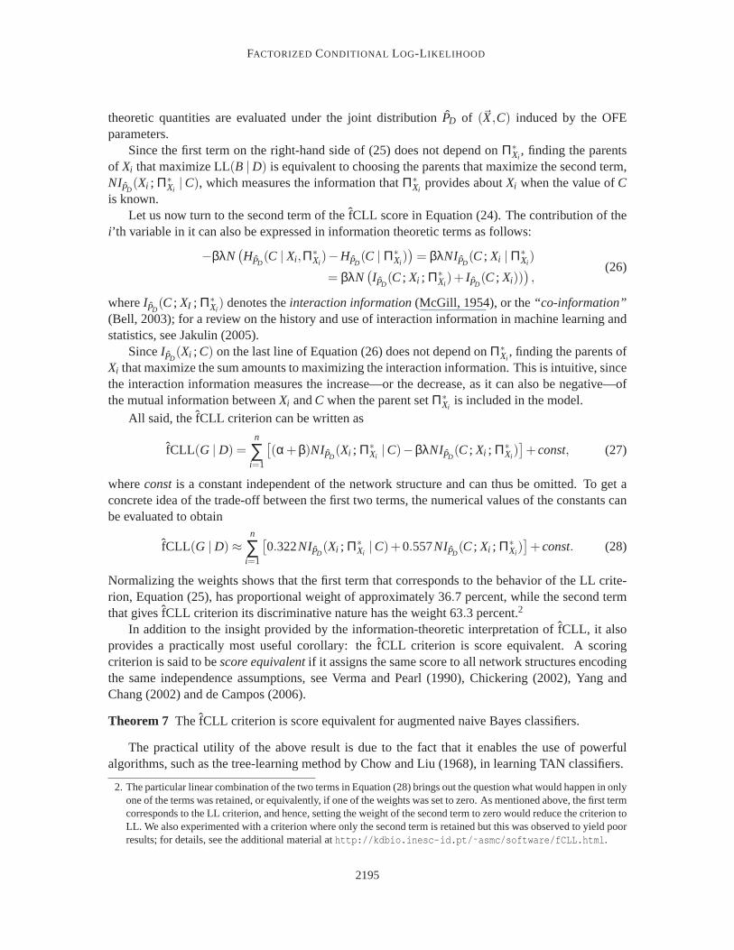
is included in the model.All said, thefCLL criterion can be written as

fCLL(G | D) =n

∑i=1

[(α+β)NIPD

(Xi ; Π∗Xi|C)−βλNIPD

(C; Xi ; Π∗Xi)]+const, (27)

whereconstis a constant independent of the network structure and can thus be omitted.To get aconcrete idea of the trade-off between the first two terms, the numerical values of the constants canbe evaluated to obtain

fCLL(G | D)≈n

∑i=1

[0.322NIPD

(Xi ; Π∗Xi|C)+0.557NIPD

(C; Xi ; Π∗Xi)]+const. (28)

Normalizing the weights shows that the first term that corresponds to the behavior of the LL crite-rion, Equation (25), has proportional weight of approximately 36.7 percent, while the second termthat givesfCLL criterion its discriminative nature has the weight 63.3 percent.2

In addition to the insight provided by the information-theoretic interpretation offCLL, it alsoprovides a practically most useful corollary: thefCLL criterion is score equivalent. A scoringcriterion is said to bescore equivalentif it assigns the same score to all network structures encodingthe same independence assumptions, see Verma and Pearl (1990), Chickering (2002), Yang andChang (2002) and de Campos (2006).

Theorem 7 ThefCLL criterion is score equivalent for augmented naive Bayes classifiers.

The practical utility of the above result is due to the fact that it enables the use of powerfulalgorithms, such as the tree-learning method by Chow and Liu (1968), in learning TAN classifiers.

2. The particular linear combination of the two terms in Equation (28) brings out the question what would happen in onlyone of the terms was retained, or equivalently, if one of the weights was set to zero. As mentioned above, the first termcorresponds to the LL criterion, and hence, setting the weight of the second term to zero would reduce the criterion toLL. We also experimented with a criterion where only the second term is retained but this was observed to yield poorresults; for details, see the additional material athttp://kdbio.inesc-id.pt/ ˜ asmc/software/fCLL.html .

2195

CARVALHO , ROOS, OLIVEIRA AND MYLLYM AKI

4.4 Beyond Binary Classification and TAN

AlthoughaCLL andfCLL scoring criteria were devised having in mind binary classification tasks,their application in multi-class problems is straightforward.3 For the case offCLL, the expression(24) does not involve the dual samples. Hence, it can be trivially adaptedfor non-binary classifica-tion tasks. On the other hand, the scoreaCLL in Equation (13) does depend on the dual samples. Toadapt it for multi-class problems, we consideredNi j (1−c)k = Ni j∗k−Ni jck andNi j (1−c) = Ni j −Ni jc .

Finally, we point out that despite being derived under the augmented naive Bayes model, thefCLL score can be readily applied to models where the class variable isnot a parent of some of theattributes. Hence, we can use it as a criterion for learning more general structures. The empiricalresults below demonstrate that this indeed leads to good classifiers.

5. Experimental Results

We implemented thefCLL scoring criterion on top of the Weka open-source software (Hall et al.,2009). Unfortunately, the Weka implementation of the TAN classifier assumes that the learningcriterion is score equivalent, which rules out the use of ouraCLL criterion. Non-score-equivalentcriteria require the Edmonds’ maximum branchings algorithm that builds a maximaldirectedspan-ning tree (see Edmonds 1967, or Lawler 1976) instead of an undirected one obtained by the Chow-Liu algorithm (Chow and Liu, 1968). Edmonds’ algorithm had already beenimplemented by someof the authors (see Carvalho et al., 2007) using Mathematica 7.0 and the Combinatorica package(Pemmaraju and Skiena, 2003). Hence, theaCLL criterion was implemented in this environment.All source code and the data sets used in the experiments, can be found atfCLL web page.4

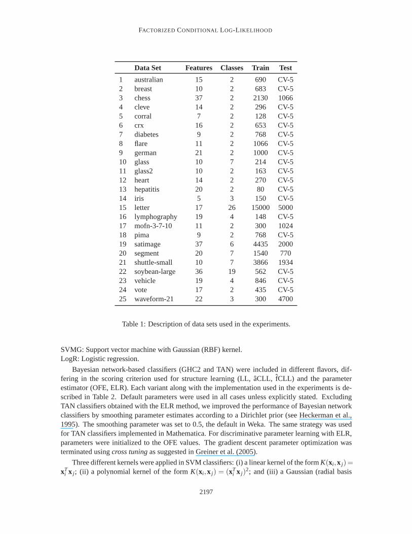
We evaluated the performance ofaCLL andfCLL scoring criteria in classification tasks compar-ing them with state-of-the-art classifiers. We performed our evaluation onthe same 25 benchmarkdata sets used by Friedman et al. (1997). These include 23 data sets fromthe UCI repository ofNewman et al. (1998) and two artificial data sets,corral andmofn, designed by Kohavi and John(1997) to evaluate methods for feature subset selection. A description ofthe data sets is presentedin Table 1. All continuous-valued attributes were discretized using the supervised entropy-basedmethod by Fayyad and Irani (1993). For this task we used the Weka package.5 Instances withmissing values were removed from the data sets.

The classifiers used in the experiments were:GHC2: Greedy hill climber classifier with up to 2 parents.TAN: Tree augmented naive Bayes classifier.C4.5: C4.5 classifier.k-NN: k-nearest neighbor classifier, withk= 1,3,5.SVM: Support vector machine with linear kernel.SVM2: Support vector machine with polynomial kernel of degree 2.

3. As suggested by an anonymous referee, the techniques used in Section 4.1 for deriving theaCLL criterion can begeneralized to the multi-class case as well as to other distributions in addition to the uniform one in a straightforwardmanner by applying results from regression theory. We plan to explore such generalizations of both theaCLL andfCLL criteria in future work.

4. fCLL web page is athttp://kdbio.inesc-id.pt/ ˜ asmc/software/fCLL.html .5. Discretization was done usingweka.filters.supervised.attribute.Discretize , with default parameters.

This discretization improved the accuracy of all classifiers used in the experiments, including those that do notnecessarily require discretization, that is, C4.5k-NN, SVM, and LogR.

2196

FACTORIZED CONDITIONAL LOG-L IKELIHOOD

Data Set Features Classes Train Test

1 australian 15 2 690 CV-52 breast 10 2 683 CV-53 chess 37 2 2130 10664 cleve 14 2 296 CV-55 corral 7 2 128 CV-56 crx 16 2 653 CV-57 diabetes 9 2 768 CV-58 flare 11 2 1066 CV-59 german 21 2 1000 CV-510 glass 10 7 214 CV-511 glass2 10 2 163 CV-512 heart 14 2 270 CV-513 hepatitis 20 2 80 CV-514 iris 5 3 150 CV-515 letter 17 26 15000 500016 lymphography 19 4 148 CV-517 mofn-3-7-10 11 2 300 102418 pima 9 2 768 CV-519 satimage 37 6 4435 200020 segment 20 7 1540 77021 shuttle-small 10 7 3866 193422 soybean-large 36 19 562 CV-523 vehicle 19 4 846 CV-524 vote 17 2 435 CV-525 waveform-21 22 3 300 4700

Table 1: Description of data sets used in the experiments.

SVMG: Support vector machine with Gaussian (RBF) kernel.LogR: Logistic regression.

Bayesian network-based classifiers (GHC2 and TAN) were included in different flavors, dif-fering in the scoring criterion used for structure learning (LL,aCLL, fCLL) and the parameterestimator (OFE, ELR). Each variant along with the implementation used in the experiments is de-scribed in Table 2. Default parameters were used in all cases unless explicitly stated. ExcludingTAN classifiers obtained with the ELR method, we improved the performance ofBayesian networkclassifiers by smoothing parameter estimates according to a Dirichlet prior (see Heckerman et al.,1995). The smoothing parameter was set to 0.5, the default in Weka. The same strategy was usedfor TAN classifiers implemented in Mathematica. For discriminative parameter learning with ELR,parameters were initialized to the OFE values. The gradient descent parameter optimization wasterminated usingcross tuningas suggested in Greiner et al. (2005).

Three different kernels were applied in SVM classifiers: (i) a linear kernel of the formK(xi ,x j)=xT

i x j ; (ii) a polynomial kernel of the formK(xi ,x j) = (xTi x j)

2; and (iii) a Gaussian (radial basis

2197

CARVALHO , ROOS, OLIVEIRA AND MYLLYM AKI

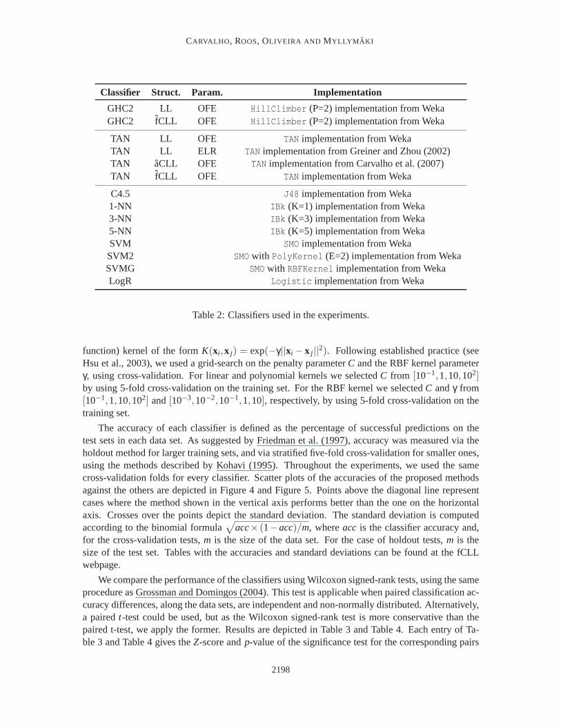
Classifier Struct. Param. Implementation

GHC2 LL OFE HillClimber (P=2) implementation from WekaGHC2 fCLL OFE HillClimber (P=2) implementation from Weka

TAN LL OFE TAN implementation from WekaTAN LL ELR TAN implementation from Greiner and Zhou (2002)TAN aCLL OFE TAN implementation from Carvalho et al. (2007)TAN fCLL OFE TAN implementation from Weka

C4.5 J48 implementation from Weka1-NN IBk (K=1) implementation from Weka3-NN IBk (K=3) implementation from Weka5-NN IBk (K=5) implementation from WekaSVM SMOimplementation from WekaSVM2 SMOwith PolyKernel (E=2) implementation from WekaSVMG SMOwith RBFKernel implementation from WekaLogR Logistic implementation from Weka

Table 2: Classifiers used in the experiments.

function) kernel of the formK(xi ,x j) = exp(−γ||xi − x j ||2). Following established practice (see

Hsu et al., 2003), we used a grid-search on the penalty parameterC and the RBF kernel parameterγ, using cross-validation. For linear and polynomial kernels we selectedC from [10−1,1,10,102]by using 5-fold cross-validation on the training set. For the RBF kernel weselectedC andγ from[10−1,1,10,102] and[10−3,10−2,10−1,1,10], respectively, by using 5-fold cross-validation on thetraining set.

The accuracy of each classifier is defined as the percentage of successful predictions on thetest sets in each data set. As suggested by Friedman et al. (1997), accuracy was measured via theholdout method for larger training sets, and via stratified five-fold cross-validation for smaller ones,using the methods described by Kohavi (1995). Throughout the experiments, we used the samecross-validation folds for every classifier. Scatter plots of the accuracies of the proposed methodsagainst the others are depicted in Figure 4 and Figure 5. Points above the diagonal line representcases where the method shown in the vertical axis performs better than the one on the horizontalaxis. Crosses over the points depict the standard deviation. The standard deviation is computedaccording to the binomial formula

√acc× (1−acc)/m, whereacc is the classifier accuracy and,

for the cross-validation tests,m is the size of the data set. For the case of holdout tests,m is thesize of the test set. Tables with the accuracies and standard deviations canbe found at the fCLLwebpage.

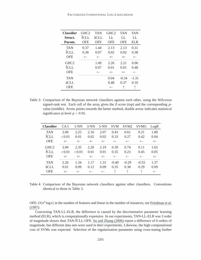
We compare the performance of the classifiers using Wilcoxon signed-rank tests, using the sameprocedure as Grossman and Domingos (2004). This test is applicable when paired classification ac-curacy differences, along the data sets, are independent and non-normally distributed. Alternatively,a pairedt-test could be used, but as the Wilcoxon signed-rank test is more conservative than thepaired t-test, we apply the former. Results are depicted in Table 3 and Table 4. Each entry of Ta-ble 3 and Table 4 gives theZ-score andp-value of the significance test for the corresponding pairs

2198

FACTORIZED CONDITIONAL LOG-L IKELIHOOD

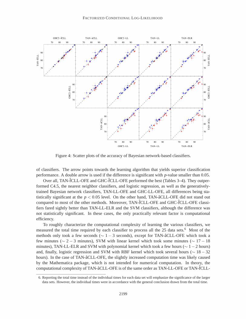
Figure 4: Scatter plots of the accuracy of Bayesian network-based classifiers.

of classifiers. The arrow points towards the learning algorithm that yields superior classificationperformance. A double arrow is used if the difference is significant withp-value smaller than 0.05.

Over all, TAN-fCLL-OFE and GHC-fCLL-OFE performed the best (Tables 3–4). They outper-formed C4.5, the nearest neighbor classifiers, and logistic regression,as well as the generatively-trained Bayesian network classifiers, TAN-LL-OFE and GHC-LL-OFE,all differences being sta-tistically significant at thep < 0.05 level. On the other hand, TAN-aCLL-OFE did not stand outcompared to most of the other methods. Moreover, TAN-fCLL-OFE and GHC-fCLL-OFE classi-fiers fared sightly better than TAN-LL-ELR and the SVM classifiers, although the difference wasnot statistically significant. In these cases, the only practically relevant factor is computationalefficiency.

To roughly characterize the computational complexity of learning the variousclassifiers, wemeasured the total time required by each classifier to process all the 25 data sets.6 Most of themethods only took a few seconds (∼ 1− 3 seconds), except for TAN-aCLL-OFE which took afew minutes (∼ 2− 3 minutes), SVM with linear kernel which took some minutes (∼ 17− 18minutes), TAN-LL-ELR and SVM with polynomial kernel which took a few hours (∼ 1−2 hours)and, finally, logistic regression and SVM with RBF kernel which took several hours (∼ 18− 32hours). In the case of TAN-aCLL-OFE, the slightly increased computation time was likely causedby the Mathematica package, which is not intended for numerical computation.In theory, thecomputational complexity of TAN-aCLL-OFE is of the same order as TAN-LL-OFE or TAN-fCLL-

6. Reporting the total time instead of the individual times for each data set willemphasize the significance of the largerdata sets. However, the individual times were in accordance with the general conclusion drawn from the total time.

2199

CARVALHO , ROOS, OLIVEIRA AND MYLLYM AKI

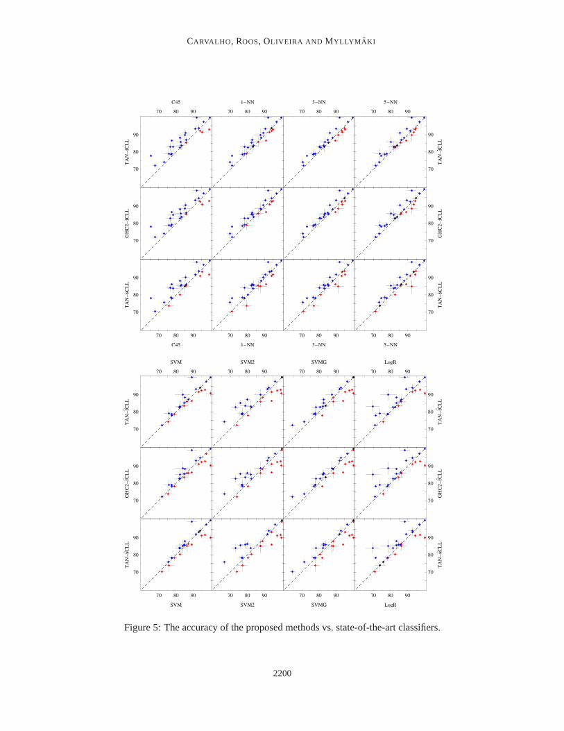
Figure 5: The accuracy of the proposed methods vs. state-of-the-artclassifiers.

2200

FACTORIZED CONDITIONAL LOG-L IKELIHOOD

Classifier GHC2 TAN GHC2 TAN TANStruct. fCLL aCLL LL LL LLParam. OFE OFE OFE OFE ELR

TAN 0.37 1.44 2.13 2.13 0.31fCLL 0.36 0.07 0.02 0.02 0.38OFE ← ← ⇐ ⇐ ←

GHC2 1.49 2.26 2.21 0.06fCLL 0.07 0.01 0.01 0.48OFE ← ⇐ ⇐ ←

TAN 0.04 -0.34 -1.31aCLL 0.48 0.37 0.10OFE ← ↑ ↑

Table 3: Comparison of the Bayesian network classifiers against each other, using the Wilcoxonsigned-rank test. Each cell of the array gives theZ-score (top) and the correspondingp-value (middle). Arrow points towards the better method, double arrow indicates statisticalsignificance at levelp< 0.05.

Classifier C4.5 1-NN 3-NN 5-NN SVM SVM2 SVMG LogR

TAN 3.00 2.25 2.16 2.07 0.43 0.61 0.21 1.80fCLL <0.01 0.01 0.02 0.02 0.33 0.27 0.42 0.04OFE ⇐ ⇐ ⇐ ⇐ ← ← ← ⇐

GHC2 3.00 2.35 2.20 2.19 0.39 0.74 0.11 1.65fCLL <0.01 <0.01 0.01 0.01 0.35 0.23 0.45 0.05OFE ⇐ ⇐ ⇐ ⇐ ← ← ← ⇐

TAN 2.26 1.34 1.17 1.31 -0.40 -0.29 -0.55 1.37aCLL 0.01 0.09 0.12 0.09 0.35 0.38 0.29 0.09OFE ⇐ ← ← ← ↑ ↑ ↑ ←

Table 4: Comparison of the Bayesian network classifiers against other classifiers. Conventionsidentical to those in Table 3.

OFE:O(n2 logn) in the number of features and linear in the number of instances, see Friedmanet al.(1997).

Concerning TAN-LL-ELR, the difference is caused by the discriminative parameter learningmethod (ELR), which is computationally expensive. In our experiments, TAN-LL-ELR was 3 orderof magnitude slower than TAN-fCLL-OFE. Su and Zhang (2006) report a difference of 6 orders ofmagnitude, but different data sets were used in their experiments. Likewise, the high computationalcost of SVMs was expected. Selection of the regularization parameter using cross-tuning further

2201

CARVALHO , ROOS, OLIVEIRA AND MYLLYM AKI

increases the cost. In our experiments, SVMs were clearly slower thanfCLL-based classifiers.Furthermore, in terms of memory, SVMs with polynomial and RBF kernels, as well as logisticregression, required that the available memory was increased to 1 GB of memory, whereas all otherclassifiers coped with the default 128 MB.

6. Conclusions and Future Work

We proposed a new decomposable scoring criterion for classification tasks. The new score, calledfactorized conditional log-likelihood,fCLL, is based on an approximation of conditionallog-likelihood. The new criterion is decomposable, score-equivalent, and allows efficient estima-tion of both structure and parameters. The computational complexity of the proposed method isof the same order as the traditional log-likelihood criterion. Moreover, the criterion is specificallydesigned for discriminative learning.

The merits of the new scoring criterion were evaluated and compared to thoseof common state-of-the-art classifiers, on a large suite of benchmark data sets from the UCI repository. OptimalfCLL-scored tree-augmented naive Bayes (TAN) classifiers, as wellas somewhat more generalstructures (referred to above as GHC2), performed better than generatively-trained Bayesian net-work classifiers, as well as C4.5, nearest neighbor, and logistic regression classifiers, with statisticalsignificance. Moreover,fCLL-optimized classifiers performed better, although the difference is notstatistically significant, than those where the Bayesian network parameters were optimized using anearlier discriminative criterion (ELR), as well as support vector machines(with linear, polynomialand RBF kernels). In comparison to the latter methods, our method is considerably more efficientin terms of computational cost, taking 2 to 3 orders of magnitude less time for the data sets in ourexperiments.

Directions for future work include: studying in detail the asymptotic behaviorof fCLL for TANand more general models; combining our intermediate approximation, aCLL, withdiscriminativeparameter estimation (ELR); extending aCLL andfCLL to mixture models; and applications in dataclustering.

Acknowledgments

The authors are grateful to the invaluable comments by the anonymous referees. The authors thankVtor Rocha Vieira, from the Physics Department at IST/TULisbon, for hisenthusiasm in cross-checking the analytical integration of the first approximation, and Mrio Figueiredo, from the Elec-trical Engineering at IST/TULisbon, for his availability in helping with concerns that appeared withrespect to this work.

The work of AMC and ALO was partially supported by FCT (INESC-ID multiannual funding)through the PIDDAC Program funds. The work of AMC was also supported by FCT and EUFEDER via project PneumoSyS (PTDC/SAU-MII/100964/2008). The work of TR and PM wassupported in part by the Academy of Finland (Projects MODEST and PRIME) and the EuropeanCommission Network of Excellence PASCAL.

Availability: Supplementary material including program code and the data sets used in the experi-ments can be found athttp://kdbio.inesc-id.pt/ ˜ asmc/software/fCLL.html .

2202

FACTORIZED CONDITIONAL LOG-L IKELIHOOD

Appendix A. Detailed Proofs

Proof (Theorem 1)We have that

Sp(α,β,γ) =

p∫

0

p∫

0

1p2

(log

(x

x+y

)− (α log(x)+β log(y)+ γ)

)2

dydx

=1

12ln(2)2(−π2(−1+α+β)

+6(2+4α2+4β2−4ln(2)−2γ ln(2)+4ln(2)2+8γ ln(2)2+2γ2 ln2(2)

+β(5−4(2+ γ) ln(2))+α(1+4β−4(2+ γ) ln(2)))

−12(α+β)(1+2α+2β−4ln(2)−2γ ln(2)) ln(p)+12(α+β)2 ln2(p)).

Moreover,∇.Sp = 0 iff

α =π2+6

24,

β =π2−18

24,

γ =π2

12ln(2)−

(2+

(π2−6) log(p)12

),

which coincides exactly with (8), (9) and (10), respectively. Now to show that (8), (9) and (10)define a global minimum, takeδ = (α log(p)+β log(p)+ γ) and notice that

Sp(α,β,γ) =

p∫

0

p∫

0

1p2

(log

(x

x+y

)− (α log(x)+β log(y)+ γ)

)2

dydx

=

1∫

0

1∫

0

1p2

(log

(px

px+ py

)− (α log(px)+β log(py)+ γ)

)2

p2dydx

=

1∫

0

1∫

0

(log

(x

x+y

)− (α log(x)+β log(y)+(α log(p)+β log(p)+ γ))

)2

dydx

=

1∫

0

1∫

0

(log

(x

x+y

)− (α log(x)+β log(y)+δ)

)2

dydx

= S1(α,β,δ).

So,Sp has a minimum at (8), (9) and (10) iffS1 has a minimum at (8), (9) and

δ =π2

12ln(2)−2.

The Hessian ofS1 is

4ln2(2)

2ln2(2)

− 2ln(2)

2ln2(2)

4ln2(2)

− 2ln(2)

− 2ln(2) −

2ln(2) 2

2203

CARVALHO , ROOS, OLIVEIRA AND MYLLYM AKI

and its eigenvalues are

rcle1 =3+ ln2(2)+

√9+2ln2(2)+ ln(2)4

ln2(2),

e2 =2

ln2(2),

e3 =3+ ln2(2)−

√9+2ln2(2)+ ln(2)4

ln2(2),

which are all positive. Thus,S1 has a local minimum in(α,β,δ) and, consequently,Sp has a localminimum in(α,β,γ). Since∇.Sp has only one zero,(α,β,γ) is a global minimum ofSp. �

Proof (Theorem 2)We have that

p∫

0

p∫

0

1p2

(log

(x

x+y

)− (α log(x)+β log(y)+ γ)

)dydx= 0

for α,β andγ defined as in (8), (9) and (10). Since the MSE coincides with the variancefor anyunbiased estimator, the proposed approximation is the one with minimum variance. �

Proof (Theorem 3)We have that

√√√√√p∫

0

p∫

0

1p2

(log

(x

x+y

)− (α log(x)+β log(y)+ γ)

)2

dydx=

√36+36π2−π4

288ln2(2)−2

for α,β andγ defined as in (8), (9) and (10), which concludes the proof. �

For the proof of Theorem 4, we recall Gibb’s inequality.

Lemma 8 (Gibb’s inequality) Let P(x) andQ(x) be two probability distributions over the samedomain, then

∑x

P(x) log(Q(x))≤∑x

P(x) log(P(x)).

Proof (Theorem 4)We now take advantage of Gibb’s inequality to show that the parameters thatmaximize thef (B | D) are those given by the OFE. Observe that

f (B | D) = λn

∑i=1

q∗i

∑j=1

r i

∑k=1

1

∑c=0

Ni jck log

(Ni jcθi jck

Ni jcθi jck +Ni j (1−c)θi j (1−c)k

)− log

(Ni jc

Ni j∗

)

= K+λn

∑i=1

q∗i

∑j=1

r i

∑k=1

Ni j∗k

1

∑c=0

Ni jck

Ni j∗klog

(Ni jcθi jck

Ni jcθi jck +Ni j (1−c)θi j (1−c)k

), (29)

2204

FACTORIZED CONDITIONAL LOG-L IKELIHOOD

whereK is a constant that does not depend on the parametersθi jck, and therefore, can be ignored.Moreover, if we take the OFE for the parameters, we have

θi jck =Ni jkc

Ni jcand θi j (1−c)k =

Ni jk(1−c)

Ni j (1−c).

By plugging the OFE estimates in (29) we obtain

f (G | D) = K+λn

∑i=1

q∗i

∑j=1

r i

∑k=1

Ni j∗c

1

∑c=0

Ni jck

Ni j∗klog

Ni jc

Ni jck

Ni jc

Ni jcNi jck

Ni jc+Ni j (1−c)

Ni j (1−c)k

Ni j (1−c)

= K+λn

∑i=1

qi

∑j=1

r i

∑k=1

Ni j∗k

1

∑c=0

Ni jck

Ni j∗klog

(Ni jck

Ni j∗k

).

According to Gibb’s inequality, this is the maximum value thatf (B | D) can attain, and therefore,the parameters that maximizef (B | D) are those given by the OFE. �

Proof (Theorem 5)We have that

S(λ,ρ) =1∫

0

(log

(x

1−x

)− (λ log(x)+ρ)

)2

dx=6λ2+π2+3ρ2 ln2(2)−λ

(π2+6ρ ln(2)

)

3ln2(2).

Moreover∇.S= 0 iffλ = π2

6 ,

ρ = π2

6ln(2) ,

which coincides with (18) and (19), respectively. The Hessian ofS is(

4ln2(2)

− 2ln(2) ,

− 2ln(2) 2

)

with eigenvalues

2+ ln2(2)±√

4+ ln4(2)

ln2(2)

which are both positive. Hence, there is only one minimum, and(λ,ρ) is the global minimum. �

Proof (Theorem 6)We have that

1∫

0

(log

(x

1−x

)− (λ log(x)+ρ)

)dx= 0

for λ andρ defined as in Equations (18) and (19). Since the MSE coincides with the variance forany unbiased estimator, the proposed approximation is the one with minimum variance. �

Proof (Theorem 7)By Theorem 2 in Chickering (1995), it is enough to show that for graphsG1

andG2 differing only on reversing one covered edge, we have thatfCLL(G1 | D) = fCLL(G2 | D).

2205

CARVALHO , ROOS, OLIVEIRA AND MYLLYM AKI

Assume thatX→Y occurs inG1 andY→ X occurs inG2 and thatX→Y is covered, that is,ΠG1

Y = ΠG1X ∪{X}. Since we are only dealing with augment naive Bayes classifiers,X andY are

different fromC and so we also haveΠ∗G1Y = Π∗G1

X ∪{X}. Moreover, takeG0 to be the graphG1

without the edgeX→Y (which is the same as graphG2 without the edgeY→ X). Then, we havethatΠ∗G0

X = Π∗G0Y = Π∗G0 and, moreover, the following equalities hold:

Π∗G1X = Π∗G0; Π∗G2

Y = Π∗G0;

Π∗G1Y = Π∗G0∪{X}; Π∗G2

X = Π∗G0∪{Y}.

SincefCLL is a local scoring criterion,fCLL(G1 | D) can be computed fromfCLL(G0 | D) takingonly into account the difference in the contribution of nodeY. In this case, by Equation (27), itfollows that

fCLL(G1 | D) = fCLL(G0 | D)− ((α+β)NIPD(Y;Π∗G0 |C)−βλNIPD

(Y;Π∗G0;C))

+((α+β)NIPD(Y;Π∗G1

Y |C)−βλNIPD(Y;Π∗G1

Y ;C))

= fCLL(G0 | D)+(α+β)N(IPD(Y;Π∗G0∪{X} |C)− IPD

(Y;Π∗G0 |C))

−βλN(IPD(Y;Π∗G0∪{X};C)− IPD

(Y;Π∗G0;C))

and, similarly, that

fCLL(G2 | D) = fCLL(G0 | D)+(α+β)N(IPD(X;Π∗G0∪{Y} |C)− IPD

(X;Π∗G0 |C))+

−βλN(IPD(X;Π∗G0∪{Y};C)− IPD

(X;Π∗G0;C)).

To show thatfCLL(G1 | D) = fCLL(G2 | D) it suffices to prove that

IPD(Y;Π∗G0∪{X} |C)− IPD

(Y;Π∗G0 |C) = IPD(X;Π∗G0∪{Y} |C)− IPD

(X;Π∗G0 |C) (30)

and that

IPD(Y;Π∗G0∪{X};C)− IPD

(Y;Π∗G0;C) = IPD(X;Π∗G0∪{Y};C))− IPD

(X;Π∗G0;C). (31)

We start by showing (30). In this case, by definition of conditional mutual, we have that

IPD(Y;Π∗G0∪{X} |C)− IPD

(Y;Π∗G0 |C) =

= HPD(Y |C)+HPD

(Π∗G0∪{X} |C)−HPD(Π∗G0∪{X,Y} |C)−HPD

(Y |C)+

−HPD(Π∗G0 |C)+HPD

(Π∗G0∪{Y} |C)

=−HPD(Π∗G0 |C)+HPD

(Π∗G0∪{X} |C)+HPD(Π∗G0∪{Y} |C)−HPD

(Π∗G0∪{X,Y} |C)

= IPD(X;Π∗G0∪{Y} |C)− IPD

(X;Π∗G0 |C).

Finally, each term in (31) is, by definition, given by

IPD(Y;Π∗G0∪{X};C) = IPD

(Y;Π∗G0∪{X} |C)− IPD(Y;Π∗G0∪{X})

︸ ︷︷ ︸E1

IPD(Y;Π∗G0;C) = IPD

(Y;Π∗G0 |C)− IPD(Y;Π∗G0)

︸ ︷︷ ︸E2

IPD(X;Π∗G0∪{Y};C) = IPD

(X;Π∗G0∪{Y} |C)− IPD(X;Π∗G0∪{Y})

︸ ︷︷ ︸E3

IPD(X;Π∗G0;C) = IPD

(X;Π∗G0 |C)− IPD(X;Π∗G0

︸ ︷︷ ︸E4

).

2206

FACTORIZED CONDITIONAL LOG-L IKELIHOOD

Since by definition of mutual information we have that

IPD(Y;Π∗G0∪{X})− IPD

(Y;Π∗G0) =

= HPD(Y)+HPD

(Π∗G0∪{X})−HPD(Π∗G0∪{X,Y})−HPD

(Y)−HPD(Π∗G0)+

+HPD(Π∗G0∪{Y})

=−HPD(Π∗G0)+HPD

(Π∗G0∪{X})+HPD(Π∗G0∪{Y})−xHPD

(Π∗G0∪{X,Y})

= IPD(X;Π∗G0∪{Y})− IPD

(X;Π∗G0),

we know thatE1−E2 = E3−E4. Thus, to prove the identity (31) it remains to show that

IPD(Y;Π∗G0∪{X} |C)− IPD

(Y;Π∗G0 |C) = IPD(X;Π∗G0∪{Y} |C)− IPD

(X;Π∗G0 |C),

which was already shown (in Equation (30)). This concludes the proof. �

Appendix B. Alternative Justification for Assumption 1

Observe that in the case at hand, we have some information aboutUt andVt , namely the number oftimes, sayNUt andNVt , respectively, thatUt andVt occur in the data setD. Moreover, we also havethe number of times, sayNRt = N− (NUt +NVt ), thatRt is found inD. Given these observations, theposterior distribution of(Ut ,Vt) under a uniform prior is

(Ut ,Vt)∼ Dirichlet(NUt +1,NVt +1,NRt +1). (32)

Furthermore, we know thatNUt andNVt are, in general, a couple (or more) orders of magnitudesmaller thanNRt . Due to this fact, most of all probability mass of (32) is found in the square[0, p]× [0, p] for some smallp.

Take as an example the (typical) case whereNUt = 1, NVt = 0, N = 500 and

p= E[Ut ]+√

Var[Ut ]≈ E[Vt ]+√

Var[Vt ],

and compare the cumulative distribution of Uniform([0, p]× [0, p]) with the cumulative distributionof Dirichlet(NUt +1,NVt +1,NRt +1). (We provide more details in the supplementary material web-page.) WheneverNRt is much larger thanNUt andNVt , the cumulative distribution Dirichlet(NUt +1,NVt +1,NRt +1) is close to that of the uniform distribution Uniform([0, p]× [0, p]) for some smallp, and hence, we obtain approximately Assumption 1.

Concerning independence, and by assuming that the distribution of(Ut ,Vt) is given by Equa-tion (32), it results from the neutrality property of the Dirichlet distribution that

Vt ⊥⊥Ut

1−Vt.

SinceVt is very small we have

Vt ⊥⊥Ut

1−Vt≈Ut .

Therefore, it is reasonable to assume thatUt andVt are (approximately) independent.

2207

CARVALHO , ROOS, OLIVEIRA AND MYLLYM AKI

References

A. J. Bell. The co-information lattice. InProc. ICA’03, pages 921–926, 2003.

J. Bilmes. Dynamic Bayesian multinets. InProc. UAI’00, pages 38–45. Morgan Kaufmann, 2000.

A. M. Carvalho. Scoring function for learning Bayesian networks. Technical report, INESC-IDTec. Rep. 54/2009, 2009.

A. M. Carvalho, A. L. Oliveira, and M.-F. Sagot. Efficient learning of Bayesian network classifiers:An extension to the TAN classifier. In M. A. Orgun and J. Thornton, editors,Proc. IA’07, volume4830 ofLNCS, pages 16–25. Springer, 2007.

D. M. Chickering. A transformational characterization of equivalent Bayesian network structures.In Proc. UAI’95, pages 87–98. Morgan Kaufmann, 1995.

D. M. Chickering. Learning Bayesian networks is NP-complete. In D. Fisher and H.-J. Lenz,editors,Learning from Data: AI and Statistics V, pages 121–130. Springer, 1996.

D. M. Chickering. Learning equivalence classes of Bayesian-network structures.Journal of Ma-chine Learning Research, 2:445–498, 2002.

D. M. Chickering, D. Heckerman, and C. Meek. Large-sample learning of Bayesian networks isNP-hard.Journal of Machine Learning Research, 5:1287–1330, 2004.

C. K. Chow and C. N. Liu. Approximating discrete probability distributions with dependence trees.IEEE Transactions on Information Theory, 14(3):462–467, 1968.

T. Cover and J. Thomas.Elements of Information Theory. John Wiley & Sons, 2006.

S. Dasgupta. Learning polytrees. InProc. UAI’99, pages 134–141. Morgan Kaufmann, 1999.

L. M. de Campos. A scoring function for learning Bayesian networks based on mutual informationand conditional independence tests.Journal of Machine Learning Research, 7:2149–2187, 2006.

P. Domingos and M. J. Pazzani. On the optimality of the simple Bayesian classifierunder zero-oneloss.Machine Learning, 29(2–3):103–130, 1997.

J. Edmonds. Optimum branchings.Journal of Research of the National Bureau of Standards, 71B:233–240, 1967.

U. M. Fayyad and K. B. Irani. Multi-interval discretization of continuous-valued attributes forclassification learning. InProc. IJCAI’93, pages 1022–1029. Morgan Kaufmann, 1993.

N. Friedman, D. Geiger, and M. Goldszmidt. Bayesian network classifiers.Machine Learning, 29(2-3):131–163, 1997.

R. Greiner and W. Zhou. Structural extension to logistic regression: Discriminative parameterlearning of belief net classifiers. InProc. AAAI/IAAI’02, pages 167–173. AAAI Press, 2002.

R. Greiner, X. Su, B. Shen, and W. Zhou. Structural extension to logisticregression: Discriminativeparameter learning of belief net classifiers.Machine Learning, 59(3):297–322, 2005.

2208

FACTORIZED CONDITIONAL LOG-L IKELIHOOD

D. Grossman and P. Domingos. Learning Bayesian network classifiers bymaximizing conditionallikelihood. InProc. ICML’04, pages 46–53. ACM Press, 2004.

M. Hall, E. Frank, G. Holmes, B. Pfahringer, P. Reutemann, and I. H. Witten. The WEKA datamining software: An update.SIGKDD Explorations, 11(1):10–18, 2009.

D. Heckerman, D. Geiger, and D. M. Chickering. Learning Bayesian networks: The combinationof knowledge and statistical data.Machine Learning, 20(3):197–243, 1995.

C.-W. Hsu, C.-C. Chang, and C.-J. Lin. A practical guide to support vector classification. Technicalreport, Department of Computer Science, National Taiwan University, 2003.

A. Jakulin.Machine Learning Based on Attribute Interactions. PhD thesis, University of Ljubljana,2005.

R. Kohavi. A study of cross-validation and bootstrap for accuracy estimation and model selection.In Proc. IJCAI’95, pages 1137–1145. Morgan Kaufmann, 1995.

R. Kohavi and G. H. John. Wrappers for feature subset selection.Artificial Intelligence, 97(1-2):273–324, 1997.

P. Kontkanen, P. Myllymaki, T. Silander, and H. Tirri. BAYDA: Software for Bayesian classificationand feature selection. InProc. KDD’98, pages 254–258. AAAI Press, 1998.

E. Lawler.Combinatorial Optimization: Networks and Matroids. Dover, 1976.

W. J. McGill. Multivariate information transmission.Psychometrika, 19:97–116, 1954.

C. Meek. Finding a path is harder than finding a tree.Journal of Artificial Intelligence Research,15:383–389, 2001.

D. J. Newman, S. Hettich, C. L. Blake, and C. J. Merz. UCI repository ofmachine learningdatabases, 1998. URLhttp://www.ics.uci.edu/ ˜ mlearn/MLRepository.html .

J. Pearl.Probabilistic Reasoning in Intelligent Systems: Networks of Plausible Inference. MorganKaufmann, San Francisco, CA, USA, 1988.

S. V. Pemmaraju and S. S. Skiena.Computational Discrete Mathematics: Combinatorics and GraphTheory with Mathematica. Cambridge University Press, 2003.

F. Pernkopf and J. A. Bilmes. Discriminative versus generative parameter and structure learning ofBayesian network classifiers. InProc. ICML’05, pages 657–664. ACM Press, 2005.

T. Roos, H. Wettig, P. Grunwald, P. Myllymaki, and H. Tirri. On discriminative Bayesian networkclassifiers and logistic regression.Machine Learning, 59(3):267–296, 2005.

T. Silander, T. Roos, and P. Myllymaki. Learning locally minimax optimal Bayesian networks.International Journal of Approximate Reasoning, 51(5):544–557, 2010.

J. Su and H. Zhang. Full Bayesian network classifiers. InProc. ICML’06, pages 897–904. ACMPress, 2006.

2209

CARVALHO , ROOS, OLIVEIRA AND MYLLYM AKI

J. Su, H. Zhang, C. X. Ling, and S. Matwin. Discriminative parameter learning for Bayesian net-works. InProc ICML’08, pages 1016–1023. ACM Press, 2008.

T. Verma and J. Pearl. Equivalence and synthesis of causal models. InProc. UAI’90, pages 255–270.Elsevier, 1990.

S. Yang and K.-C. Chang. Comparison of score metrics for Bayesian network learning. IEEETransactions on Systems, Man, and Cybernetics, Part A, 32(3):419–428, 2002.

2210