EUROMOD - Institute for Social and Economic … Working Paper No. EM 7/08 ... Centre for Comparative Research in the Social ... marriage market or as a horizontal equity argument that

EUROMOD

WORKING PAPER SERIES

EUROMOD Working Paper No. EM 7/08

AN EVALUATION OF THE TAX-TRANSFER TREATMENT OF MARRIED COUPLES IN EUROPEAN COUNTRIES

Herwig Immervoll

Henrik Jacobsen Kleven Claus Thustrup Kreiner

Nicolaj Verdelin

September 2008

An Evaluation of the Tax-Transfer Treatment of Married Couples in European Countries*

Herwig Immervoll

OECD, IZA, and ISER at University of Essex

Henrik Jacobsen Kleven

London School of Economics and CEPR

Claus Thustrup Kreiner

University of Copenhagen and CESifo

Nicolaj Verdelin

University of Copenhagen

*We thank Emmanuel Saez and seminar participants at the CESifo 2008 area conference on public sector economics for comments. The project has been supported by a grant from the Economic Policy Research Network (EPRN). Any remaining errors and views expressed in this article are the authors’ responsibility. In particular, the paper does not necessarily represent the views of the OECD, the governments of OECD member countries or the EUROMOD consortium. This paper uses EUROMOD versions 5A and 27A which rely on micro-data from 11 different sources for 15 countries. These are the European Community Household Panel (ECHP) made available by Eurostat; the Austrian version of the ECHP made available by the Interdisciplinary Centre for Comparative Research in the Social Sciences; the Living in Ireland Survey made available by the Economic and Social Research Institute; the Panel Survey on Belgian Households (PSBH) made available by the University of Liège and the University of Antwerp; the Income Distribution Survey made available by Statistics Finland; the Enquête sur les Budgets Familiaux (EBF) made available by INSEE; the public use version of the German Socio Economic Panel Study (GSOEP) made available by the German Institute for Economic Research (DIW), Berlin; the Survey of Household Income and Wealth (SHIW95) made available by the Bank of Italy; the Socio-Economic Panel for Luxembourg (PSELL-2) made available by CEPS/INSTEAD; the Socio-Economic Panel Survey (SEP) made available by Statistics Netherlands through the mediation of the Netherlands Organisation for Scientific Research - Scientific Statistical Agency; the Income Distribution Survey made available by Statistics Sweden; and the Family Expenditure Survey (FES), made available by the UK Office for National Statistics (ONS) through the Data Archive. Material from the FES is Crown Copyright and is used by permission. Neither the ONS nor the Data Archive bear any responsibility for the analysis or interpretation of the data reported here.

An Evaluation of the Tax-Transfer Treatment of Married Couples in European Countries

Herwig Immervoll

Henrik Jacobsen Kleven Claus Thustrup Kreiner

Nicolaj Verdelin1

Abstract

This paper presents an evaluation of the tax-transfer treatment of married couples in 15 EU countries using the EUROMOD microsimulation model. First, we show that many tax-transfer schemes in Europe feature negative jointness defined as a situation where the tax rate on one person depends negatively on the earnings of the spouse. This stands in contrast to the previous literature on this question, which has focused on a specific form of positive jointness. The presence of negative jointness is driven by family-based and means-tested transfer programs combined with tax systems that usually feature very little jointness. Second, we consider the labor supply distortion on secondary earners relative to primary earners implied by the current tax-transfer systems, and study the welfare effects of small reforms that change the relative taxation of spouses. By adopting a small-reform methodology, it is possible to set out a simple analysis based on more realistic labor supply models than those considered in the existing literature. We present microsimulations showing that simple revenue-neutral reforms that lower the tax burden on secondary earners are associated with substantial welfare gains in most countries. Finally, we consider the tax-transfer implications of marriage and estimate the so-called marriage penalty. For most countries, we find large marriage penalties at the bottom of the distribution driven primarily by features of the transfer system.

JEL Classification: H20

Keywords: labour supply, redistribution, optimal tax, couples, marriage tax, joint taxation

Corresponding author:

Henrik Kleven Department of Economics and STICERD London School of Economics and Political Science, Houghton Street, London WC2A 2AE, United Kingdom E-mail: [email protected]

1 This paper was written as part of a project financed by the Economic Policy Research Network (EPRN). We are indebted to all past and current members of the EUROMOD consortium for the construction and development of EUROMOD. We also wish to thank Emmanuel Saez and seminar participants at the CESifo 2008 area conference on public sector economics for providing valuable comments on earlier drafts. However, any errors and the views expressed in this paper are the authors' responsibility. In particular, the paper does not represent the views of the institutions to which the authors are affiliated.

1 Introduction

The tax treatment of couples has been a debating point throughout the existence of the income

tax. Actual policies have varied over time and across countries. Over the past three decades,

there has been an international trend from joint to individual taxation of husbands and wives,

and today the majority of OECD countries use the individual as the basic unit of taxation.

Under fully individual taxation, tax liability is assessed separately for each family member and

is therefore independent of the income of other individuals living in the household. By contrast,

in a system of fully joint taxation of couples, as operated by for example the United States, tax

liability is assessed at the family level and depends on total family income. Three basic points

have been noted in previous discussions of the choice between individual and joint taxation (e.g.,

Rosen, 1977; Boskin and Sheshinski, 1983; Pechman, 1987).

The first argument is an efficiency argument. It starts from the empirical observation that

the secondary earner in a family–typically the wife–tends to have a more elastic labor supply

than the primary earner (e.g., Blundell and MaCurdy, 1999). A Ramsey-type optimal tax rule

then suggests that the labor income of secondary earners should be taxed at a lower rate than the

labor income of primary earners. This is achieved to a certain degree by a progressive individual

income tax, because primary earners have higher incomes and therefore face higher marginal tax

rates than their spouses. On the other hand, a fully joint income tax creates identical marginal

tax rates across members of the same household and hence does not meet this efficiency criterion.

The second argument is that tax systems should be neutral with respect to marriage deci-

sions. This can be viewed as an efficiency argument that tax systems should not distort the

marriage market or as a horizontal equity argument that identical couples (married or cohabitat-

ing) should be treated identically for tax purposes. While individual-based taxation is neutral

with respect to marriage, joint tax systems are generically non-neutral. Jointness may penalize

or subsidize marriage depending on the exact design, and the size of penalties/subsidies generally

depends on the distribution of income within the family.

The third argument is an equity argument, taking as its point of departure that welfare is

better measured by family income than individual income. As a result, two families with the

same total income should, other things being the same, pay equal taxes. By the same token, if

one family receives a higher total income than another family, then the first family should face a

higher tax liability than the second one. This equity criterion is satisfied by a joint income tax

that depends on total family income, but not by a progressive individual tax system, because

in that case tax liability depends also on the distribution of incomes within the family.

This paper attempts to shed light on the three issues discussed above. We start by noting

that these issues ultimately pertain to the redistribution scheme as a whole, not just the tax

1

system, and we therefore present an integrated treatment of the tax and transfer system. A

recurrent theme in the paper is that the transfer system is a crucial element in understanding

and evaluating redistribution schemes affecting married couples. We also point out that the

focus in previous discussions on the choice between individual tax treatment and joint tax treat-

ment based on family income represents an oversimplification, because real-world redistribution

schemes are almost never fully individual or fully joint. There are two reasons for this. First,

while most countries have adopted individual filing in the tax system, they tend to retain cer-

tain elements of jointness such as the transfer of unused allowances across spouses, dependent

spouse exemptions, etc. Second, transfer systems are nearly always fully joint, because social

benefits are means-tested according to the combined income and assets of the two spouses in the

household. This implies that actual redistribution systems typically combine a form of quasi-

individual taxation with family-based transfer systems, creating a fairly complicated jointness

structure that is different from the two polar cases typically analyzed.

This paper presents a comprehensive evaluation of the tax-transfer treatment of married

couples in 15 EU countries. The analysis has three components. First, we carefully map the

nature of jointness in tax-transfer schemes in our sample of countries using the EUROMOD

microsimulation model. EUROMOD is built around country-specific, but partly harmonized,

micro datasets combined with a detailed tax-benefit simulator capturing the full set of institu-

tional features of tax and transfer systems in each country.1 We find that many tax-transfer

schemes in Europe feature negative jointness defined as a situation where the tax rate on one

person depends negatively on the earnings of the spouse. Such a system is opposite to the form

of jointness typically analyzed in the literature–fully joint and progressive taxation–because

such schemes feature a positive interaction between tax rates and spousal earnings and therefore

positive jointness. The presence of negative jointness is driven by family-based and means-tested

transfers combined with individual or almost-individual taxes. To see this, consider a secondary

earner, say the wife, deciding about labor market entry. If she is married to a low-income hus-

band, the family is in the phase-out range of transfer programs, and she will face a high effective

tax rate. On the other hand, if she is married to a high-income husband, the family is beyond

the phase-out range of transfer programs, and she will face a low effective tax rate because the

income tax is individual. Hence, the wife’s tax is declining in the husband’s earnings.

Second, the paper considers the incentives to supply labor for secondary earners relative to

primary earners implied by the existing tax-transfer systems, and studies the welfare effects of

reforms that change the relative taxation of spouses. This issue is separate from the nature

of jointness discussed above: jointness has to do with the relationship between tax rates and

1An introduction to EUROMOD and a descriptive analysis of taxes and transfers in the EU countries has beenprovided by Sutherland (2001), Immervoll and O’Donoghue (2003), and Immervoll (2004).

2

spousal earnings (a cross-derivative in the tax function), whereas labor supply incentives have

to do with the relationship between tax liability and own earnings (an own-derivative in the

tax function). Previous work has often discussed the two issues as if they are one and the

same, but we find that the distinction is important in practice. To study the welfare effects of

tax-transfer reform, the paper starts by setting out a simple theoretical model that incorporates

only participation responses, and then turn to a general model that allows for both participation

and hours-of-work responses for both spouses in the household. Microsimulations of different

revenue-neutral reforms that reduce the tax burden on secondary earners show that, for both

models and for most countries, a lowering of the tax burden on secondary earners is associated

with substantial welfare gains.

This part of the paper may be seen as an extension of our previous work based on single-

person households (Immervoll et al., 2007) to the case of two-person households. It is also

related to the recent work by Alesina and Ichino (2007), arguing that tax schemes should be

gender-specific with lower rates on females. We do not consider gender-specific taxation as

such (consistent with real-world tax systems that are anonymous and hence gender-blind), but

consider reforms that change the taxation of primary versus secondary earners. We define

primary versus secondary, not in terms of gender, but in terms of relative earnings within

the family–a concept that is correlated with gender.2 Indeed, it is shown that in almost

all countries more than 80% of secondary earners are women, and in some countries more

than 90% of secondary earners are women. Thus, the reforms under consideration strongly

target married women with low earnings or weak labor market attachment without formally

discriminating based on gender. This is important because gender-specific taxation per se would

be unconstitutional in most countries.

Third, the paper explores the distortions in the decision to marry by simulating the size of

marriage penalties resulting from the combined effect of taxes and transfers. The presence of

family-based and means-tested transfers penalizes marriage at the bottom of the distribution,

implying that marriage penalties at the bottom tend to go hand in hand with negative jointness.3

Indeed, we find large marriage penalties at the bottom of the distribution (but not at the top)

in most countries, which raises important questions pertaining to fairness as well as to efficiency.

Transfers and taxes that depend on marriage are often accused by conservatives of destroying the

traditional two-parent family and leading to high rates of single motherhood. Although empirical

studies of the effects on marriage and divorce from income taxes (e.g. Alm and Whittington,

2More specifically, the lower-earning spouse in each family is defined as the secondary earner. For one-earnercouples, this obviously implies that the non-working spouse is the secondary earner.

3However, theoretically it is entirely possible to design a negatively joint tax system that subsidizes ratherthan penalizes marriage.

3

1997, 1999), welfare benefits (e.g., Hoynes 1997a,b; Moffitt, 1998), or taxes and benefits combined

(Dickert-Conlin, 1999; Eissa and Hoynes, 2000b) tend to find modest or no effects, the existence

of marriage disincentives continues to be a controversial point of contention.

Most of the literature studying the optimal design of tax and transfer programs and the

evaluation of tax and welfare reform rests on models of single-person households. However, real-

world tax-transfer schemes for a large part redistribute income across families formed around

couples, creating a substantial gap between theory and practice. This has triggered a recent

and growing interest in generalizing the theory of optimal income redistribution to explicitly

deal with couples. For example, Kleven, Kreiner, and Saez (2007, 2008) explore the optimal

nonlinear taxation of couples as a multi-dimensional screening problem, whereby agents (couples)

are characterized by a multi-dimensional parameter (ability and taste-for-work parameters of

each spouse) that are unobserved by the principal (the government which maximizes social

welfare). They find that, under certain assumptions, optimal incentive schemes feature negative

jointness, which is consistent with our findings for Europe. Recent papers by Brett (2006) and

Cremer, Lozachmeur and Pestieau (2006) also analyze the optimal taxation of couples as a

multidimensional screening problem. The rest of the literature (e.g. Schroyen, 2003; Alesina

and Ichino, 2007) typically restricts the tax function to be separable (albeit gender-specific),

thereby sidestepping the complexities associated with multi-dimensional screening.

Our paper may be seen as an applied counterpart to these recent theoretical papers. By

focusing on small reforms rather than the optimal system, we are able to set out a tractable

analysis based on more general and realistic labor supply models than the very stylized models

previously considered.

The paper proceeds as follows. Section 2 describes the data and the EUROMOD model.

Section 3 maps out the existing tax-transfer treatment of married couples in our sample of

European countries. Section 4 sets out a joint labor supply model to evaluate reforms affecting

married couples, and presents a microsimulation study of specific reforms that reduce the tax

burden on second-earner participation. Section 5 studies marriage penalties, and Section 6

concludes.

2 Data

Our data source is EUROMOD, a microsimulation model for the EU built around partly homog-

enized micro datasets that include data on earnings, labor force participation and demographics.

The version available for this study relates to 1998 and covers the 15 countries that constituted

the EU at that time. Based on detailed algorithms capturing the full range of institutional

features of tax and transfer systems in each country, the model is able to compute a wide

4

range of taxes and benefits for each observation unit in representative samples for the various

countries. The main policy instruments incorporated in EUROMOD are income taxes, social

security contributions (or payroll taxes) paid by employees, benefit recipients, and employers as

well as universal and means-tested social benefits including housing assistance.4 The model fully

accounts for the complicated interaction of different types of taxes and benefits with earnings,

assets, employment status, marital status, housing situation and children, and its considerable

level of detail makes it an ideal tool for comparative tax analysis.5

We restrict the sample to married couples where both husband and wife are between 16 and

64 years of age, where the couple as a whole reports positive annual earnings, and where at

least one member of the household has been working the entire year. We exclude those who are

currently receiving pension, early retirement, or disability benefits. In each couple, we define

the primary earner (PE) as the highest-earning member and the secondary earner (SE) as the

lowest-earnings member of the household. Together with our sample restriction, this implies

that, in one-earner couples, the primary earner works the entire year while the secondary earner

is non-employed throughout the year. In two-earner couples, the secondary earner works either

part of or the entire year but always has relatively low earnings.

While we feel that it makes sense to define primary versus secondary earner in terms of

earnings (and indirectly labor market participation), the earnings-based definition is in practice

highly correlated with a gender-based definition. To demonstrate this, Table 1 displays the

share of women among secondary earners according to our definition. We see that, in one-earner

couples, more than 90 percent of secondary earners (non-participants) are women in all countries

except the Nordic countries and the United Kingdom. In two-earner couples, the second-earner

definition is slightly less skewed towards women, so that on average the share of secondary earners

that are women varies between 80 and 90 percent across most of the 15 countries in our sample.

The close relationship between relative earnings within families and gender implies that a purely

earnings-based couple tax function can be targeted to gender without being formally gender-

based. This is important because gender-specific taxation per se would be unconstitutional in

most countries.6

4 In the results reported here, we do not include unemployment insurance (UI) benefits in the calculation ofeffective participation tax rates. This is due in part to difficulties associated with accounting properly for theimplications of limited UI duration in our static tax rate measures. At a more conceptual level, it is likely that UIschemes providing insurance against involuntary and temporary job loss have very different incentive implicationsthan poverty alleviation programs offering permanent income guarantees to all non-workers.

5For further information on EUROMOD, the reader is referred to Sutherland (2001) as well as the Internet athttp://www.iser.essex.ac.uk/msu/emod

6Despite the economic equivalence between gender-based taxation and affirmative action (which has beenaproved by the courts on many occations), the two policies would be viewed very differently by the courts. SeeRubenfeld (1997) for a discussion of this point in the context of race.

5

3 The Tax-Transfer Treatment of Couples in Europe

Based on EUROMOD, this section maps out the tax-transfer treatment of married couples in

our sample of European countries. As general background, Tables A1 and A2 in the appendix

summarize the most important institutional features of tax and benefit systems affecting married

couples in each country.

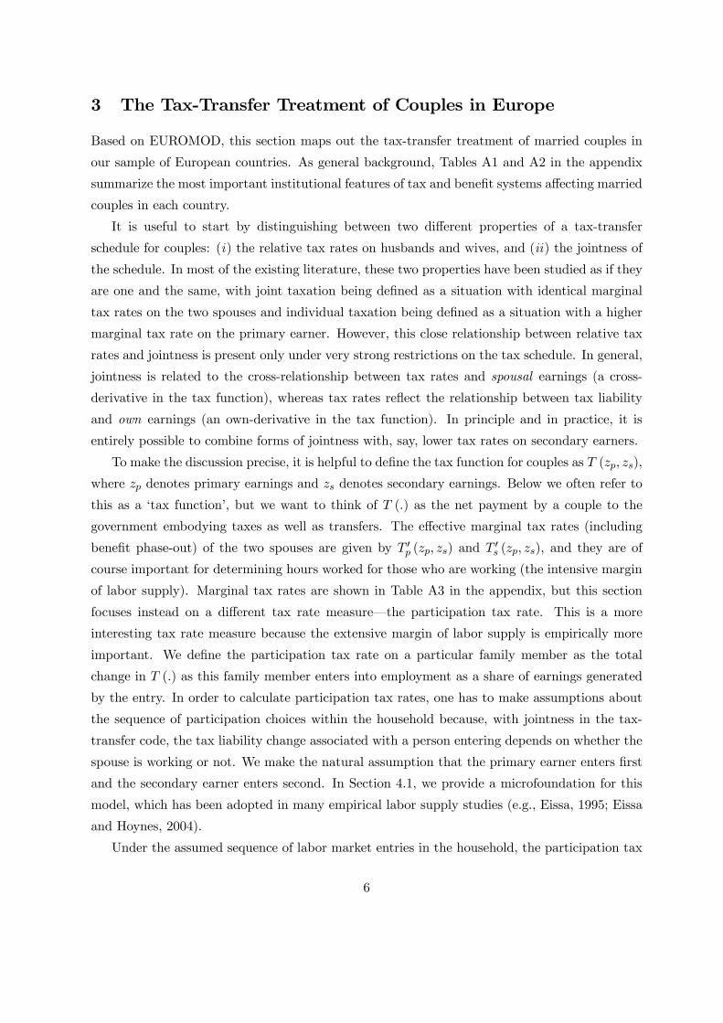
It is useful to start by distinguishing between two different properties of a tax-transfer

schedule for couples: (i) the relative tax rates on husbands and wives, and (ii) the jointness of

the schedule. In most of the existing literature, these two properties have been studied as if they

are one and the same, with joint taxation being defined as a situation with identical marginal

tax rates on the two spouses and individual taxation being defined as a situation with a higher

marginal tax rate on the primary earner. However, this close relationship between relative tax

rates and jointness is present only under very strong restrictions on the tax schedule. In general,

jointness is related to the cross-relationship between tax rates and spousal earnings (a cross-

derivative in the tax function), whereas tax rates reflect the relationship between tax liability

and own earnings (an own-derivative in the tax function). In principle and in practice, it is

entirely possible to combine forms of jointness with, say, lower tax rates on secondary earners.

To make the discussion precise, it is helpful to define the tax function for couples as T (zp, zs),

where zp denotes primary earnings and zs denotes secondary earnings. Below we often refer to

this as a ‘tax function’, but we want to think of T (.) as the net payment by a couple to the

government embodying taxes as well as transfers. The effective marginal tax rates (including

benefit phase-out) of the two spouses are given by T 0p (zp, zs) and T 0s (zp, zs), and they are of

course important for determining hours worked for those who are working (the intensive margin

of labor supply). Marginal tax rates are shown in Table A3 in the appendix, but this section

focuses instead on a different tax rate measure–the participation tax rate. This is a more

interesting tax rate measure because the extensive margin of labor supply is empirically more

important. We define the participation tax rate on a particular family member as the total

change in T (.) as this family member enters into employment as a share of earnings generated

by the entry. In order to calculate participation tax rates, one has to make assumptions about

the sequence of participation choices within the household because, with jointness in the tax-

transfer code, the tax liability change associated with a person entering depends on whether the

spouse is working or not. We make the natural assumption that the primary earner enters first

and the secondary earner enters second. In Section 4.1, we provide a microfoundation for this

model, which has been adopted in many empirical labor supply studies (e.g., Eissa, 1995; Eissa

and Hoynes, 2004).

Under the assumed sequence of labor market entries in the household, the participation tax

6

rates on the primary and secondary earners are given by

τp ≡T (zp, 0)− T (0, 0)

zp, τ s ≡

T (zp, zs)− T (zp, 0)

zs. (1)

These tax rates are simulated by EUROMOD in the following way. For the computation of

τ s, we consider the subsample of two-earner couples and start by computing actual taxes net

of transfers T (zp, zs) at each observed earnings pair, accounting for other relevant household

information (place of residence, number of kids, etc.). We then recompute taxes and transfers

in the alternative (hypothetical) situation where the secondary earner does not work, T (zp, 0),

and calculate τ s as in eq. (1). Analogously for τp, we use the sample of one-earner couples to

simulate taxes net of transfers in the original situation, T (zp, 0), and in the alternative situation

where the primary earner is not working, T (0, 0), and then apply formula (1).7

Table 2 shows participation tax rates and labor market outcomes for primary and secondary

earners in each country (averages for each country sample). As one would expect, Scandinavia

and Northern-Continental Europe feature higher overall tax rate levels than Anglo-Saxon and

Southern European countries. More interestingly, the tax rate on primary earners is higher than

on secondary earners in all but the four Southern European countries (Greece, Italy, Portugal,

and Spain). This is a result of the impact of family-based and means-tested welfare benefits,

which are affected more by the first than by the second entrant. We do not observe the same

effect in Southern Europe where welfare benefits are less generous. Although most countries

impose a higher participation tax rate on the primary earner, there are substantial differences

in the relative rates across countries. In particular, the UK system stands out by being much

more favorable to second-earner participation than all other countries.

The ratio of the primary-earner tax rate to the secondary-earner tax rate is interesting

because it can be compared to optimal tax rules expressing relative tax rates as a function of

elasticities (e.g., Boskin and Sheshinski, 1983; Kleven and Kreiner, 2006). In the special case

of separability in utility of spousal labor supplies, the optimal tax rate on each spouse is given

by an inverse elasticity rule and the optimal relative tax rate τp/τ s is therefore given by the

participation elasticity of the secondary earner relative to the primary earner. This implies that

the tax ratios in the table can be seen as critical values for relative participation elasticities.

For example, in the United Kingdom, if the second-earner elasticity is more than 2.79 times as

high as the primary earner elasticity, it would be efficient to shift some of the tax burden from

7Our tax-rate estimates are therefore calculated for those currently working. As a result of sample selection,one would expect tax rates to be different for non-working individuals considering a transition into work. As wedo not observe the earnings potential of non-working individuals, calculating their participation tax rates wouldrequire jointly estimating a wage and participation model for couples. In the microsimulation exercise in Section4, we deal with the selection issue indirectly by considering a decreasing profile of participation elasticities suchthat new labor market entrants tend to be located at the bottom end of the income distribution.

7

secondary earners to primary earners. In view of the evidence on the responsiveness of labor

force participation of married women, the table seems to suggest that in many countries the

relative tax rate on secondary earners is inefficiently high. We return to this issue in Section 4.

Finally, the table shows that both participation and earnings (conditional on participation)

tend to be strongly skewed in favor of primary earners in most countries. Although the countries

we consider differ along many dimensions (besides tax rates) that may have direct implications

for labor market outcomes, it is interesting that the cross-country variation in relative partic-

ipation is roughly consistent with the variation in relative participation taxes. For example,

Southern European countries are characterized by lower participation taxes along with higher

participation rates for primary relative to secondary earners compared to most other countries.

At the other end of the spectrum, Denmark, Finland, and the UK are associated with higher

relative tax rates and lower relative participation for primary earners.

Let us now consider the jointness of the couple tax function T (zp, zs) and therefore the

cross-derivative T 00ps. One benchmark case is that of fully individual taxation, i.e. T (zp, zs) =

Tp (zp) + Ts (zs), which is associated with a zero cross-derivative T 00ps = 0. In practice, the

functional forms Tp (.) and Ts (.) would typically be the same, in which case we have a so-called

anonymous individual tax. Another benchmark case is the fully joint couple tax T (zp + zs) as

adopted in the United States and in some European countries (see Table A1). If the system

additionally features a progressive marginal tax rate structure (T 00 > 0), the couple tax would

be associated with a positive cross-derivative T 00ps > 0. More generally, there is a whole range

of joint couple tax functions T (zp, zs) with T 00ps 6= 0. Kleven, Kreiner, and Saez (2007) define

positive jointness as a system where the tax on one person depends positively on spousal earnings

(T 00ps > 0), and negative jointness as a system where the tax on each partner depends negatively

on spousal earnings (T 00ps < 0). Because a fully joint schedule is associated with positive jointness,

individual taxation can be seen as an intermediate (rather than polar) case in between full

jointness and negative jointness. This is interesting because we show below that many real-

world schedules feature negative jointness, implying that they have moved further away from

fully joint taxation than the individual system.

The above definitions of jointness are stated in terms of cross-derivatives of marginal tax

rates. Consistent with the analysis of tax rate levels, we will state a definition of jointness in

terms of participation tax rates. In particular, we say that a system is positively joint if ∂τs∂zp> 0,

negatively joint if ∂τs∂zp< 0, and separate if ∂τs∂zp

= 0. While the definitions of jointness in terms of

marginal tax rates are local, the definitions in terms of participation (‘average’) tax rates reflect

that a tax schedule is joint on average over a range of incomes.

Before turning to the empirical results, it is helpful for a moment to separate the tax and

8

transfer system. Denote by t (zp, zs) the tax payment and by b (zp, zs) the benefit payment,

so that T (zp, zs) = t (zp, zs) − b (zp, zs). Consider then a tax-transfer scheme that combines

an individual income tax and a fully joint transfer system, i.e. T (zp, zs) = tp (zp) + ts (zs) −b (zp + zs). The definition in eq. (1) then implies τ s = [ts (zs) + b (zp)− b (zp + zs)] /zs. Means-

testing corresponds to b (zp) − b (zp + zs) ≥ 0, which creates an extra tax on second-earner

participation. However, as zp increases, the family is pushed beyond the phase-out range of the

various transfer programs (at any given zs), which tends to lower b (zp)− b (zp + zs) and create

a pattern where ∂τs∂zp

< 0 at the bottom. This explains a pattern we find for many countries.

For our measurement of jointness, we construct a number of hypothetical households that

vary with respect to household earnings and the number of children, and apply EUROMOD to

calculate effective tax rates for these hypothetical families.8 We base this part of the analysis on

hypothetical households (instead of data on actual households) in order to adequately isolate the

interdependence between spouses in the tax-benefit legislation. If we were to use sample data

and compare the net-tax burden of actual households at different earnings levels, the results

would be affected by selection effects.9

To illustrate the jointness in the tax-transfer system, we plot the participation tax rate of

married individuals at different income levels as a function of the earnings of the spouse.10

We consider married individuals at four different income levels: the 5th, 10th, 50th, and 90th

percentiles of the earnings distribution of secondary earners (denoted below by SEp5, SEp10,

SEp50, and SEp90). For each of these individual income levels, we calculate the participation tax

rate at 20 different earnings levels of the spouse, corresponding to the 5th, 10th, 15th,..., 100th

percentiles in the earnings distribution of primary earners (denoted below by PEp5, PEp10,

..., PEp100). Our results are shown in Figure 1 for families with two children. Corresponding

graphs for childless couples are provided in Figure A2 the appendix.11

The most striking result is that most countries display substantial negative jointness at the

bottom of the income distribution. As explained above, this can be largely attributed to means-

tested benefits such as social assistance, housing benefits and child benefits that are phased-out

8Because we are working with hypothetical households, it is necessary to make an assumption about the livingarrangements of the families. We have chosen to assume that all families reside in rental housing, and have thenimputed rental costs for all countries.

9For instance, marriage patterns are known to display positive assortative matching, which in itself would tendto produce a positive relationship between individual tax rates and spousal earnings.10For completeness, Figure A1 in the appendix illustrates jointness based on marginal tax rates. The qualitative

results are similar to those presented below, but participation tax rate measures are smoother because they reflectaverage jointness of marginal tax rates over a range of incomes.11When considering a couple with one spouse belonging to the bottom of the earnings distribution for primary

earners and the other spouse located at the top of the earnings distribution for secondary earners, it may actuallybe the second spouse who has the highest earnings. This is, however, only relevant for the lower part of thetwo grey curves because the earnings of the secondary earners in the data are substantially lower than primaryearnings. Moreover, the slopes of the curves still reveal the type of jointness at these earnings combinations.

9

as a function of total household income.12 Indeed, the high claw-back rates used in many

countries tend to generate participation taxes that are very high for secondary earners married

to low-wage primary earners, often above 70% and sometimes close to 100%.

Countries with negative jointness at low income levels may be divided into two groups de-

pending on the pattern at higher income levels. Countries that operate an individual income tax

(possibly apart from some family-based tax expenditures at the bottom) and/or have a fairly

flat tax rate structure at the top tend to converge towards no jointness as the income of the

primary earner becomes high.13 Austria, Denmark, Finland, Sweden and the United Kingdom

display this pattern, which we may label negative-neutral jointness. The strongest example of

this pattern is perhaps the United Kingdom where negative jointness at the bottom is driven by

both the welfare and the tax system. The Working Families Tax Credit (WFTC), an in-work

cash benefit provided through the tax system, is based on household income and is phased out

at a rate of 70%. The combination of the WFTC and the withdrawal of social assistance and

housing benefits creates participation tax rates at around 70-90% for secondary earners married

to low-income spouses. While second-earner participation in the UK is therefore strongly dis-

couraged in low-income families, it is encouraged in higher-income families due to the individual

income tax. In particular, because working spouses with low earnings are not liable to pay either

income tax and social insurance contributions, the second-earner tax rate at SEp5 and SEp10

drops to zero once primary-earner income exceeds PEp30 and stays at zero as primary earnings

increase.

Another group of countries combine negative jointness at the bottom with positive jointness

at the top. Countries with this pattern of negative-positive jointness are Belgium, France,

Germany, Ireland, Luxembourg and Portugal. All of these countries operate a progressive tax

system based on family income causing the secondary-earner participation tax to be increasing

in primary-earner income once the family is beyond the phase-out range of welfare programs.

However, the degree of positive jointness at the top is generally quite weak and much less salient

than the negative jointness at the bottom. This may seem surprising but can be explained by

the fact that the marginal tax rate structure is quite flat in most European countries, partly as a

result of upper contribution limits built into social security contribution schedules. As explained

12 In Germany and Belgium, there is an initial slight increase in the second-earner tax rate at low levels ofprimary-earner income provided that the secondary earner also enters at a low earnings level. This is becausethese countries employ an earnings disregard in the transfer system, so that the lowest-income families are notaffected by benefit withdrawal.13Notice that a flat (linear) income tax, even if it is based on family income, effectively implies separability

in the tax treatment of spouses. As an example, this is important for Denmark, which operates a form of jointtaxation by combining individual filing with the possibility of transferring certain allowances and exemptionsacross spouses. However, because the marginal tax rate structure is quite flat there is very little jointness at thetop.

10

above, a completely linear tax system, even if it is based on family income, effectively implies

separability in the tax treatment of spouses. Notice also that, in France, the curve is relatively

flat both at the bottom and at the top because the withdrawal of various family benefits and

housing assistance occurs at different income levels and tends to offset the presence of positive

jointness in the income tax.14

Greece, Italy, and to some extent the Netherlands are the only countries that show virtu-

ally no jointness. All three countries operate individual income tax systems, and in Greece

and Italy only very limited means-tested benefits are available.15 The Netherlands does offer

family-based social assistance, but primary earnings are higher in the Netherlands than in most

other countries, implying that transfer phase-out plays a limited role for second-earner labor

market entry.16 Spain is the only country characterized by positive jointness. There is no social

assistance and the design of the Spanish income tax implies that, for low-income families, it is

optimal to file under the optional joint tax. For higher-income families, it is typically optimal to

file separately, which explains why there is less jointness if the secondary earner is at the median

or above.

4 AWelfare Evaluation of Cutting Taxes for Secondary Earners

It is often argued that the tax burden on secondary earners should be reduced in order to

increase economic efficiency. Indeed, a traditional Ramsey-type efficiency argument calls for

a low marginal tax rate on secondary earners because their labor supply is relatively elastic

(Rosen, 1977; Boskin and Sheshinski, 1983). The traditional argument is derived in a model

with only hours-of-work responses and where the tax system is restricted to be linear (albeit

gender specific). However, the modern empirical labor supply literature shows that the strong

responsiveness of the labor supply of married females is driven by labor force participation, not

by hours worked for those who are working (e.g., Heckman, 1993; Blundell and MaCurdy, 1999).

This calls for a policy that reduces the participation tax rate on secondary earners.

A policy change should be evaluated, not just in terms of efficiency, but also with respect to

its consequences for distributional equity. A revenue-neutral reform reducing the participation

14 In France, the drop in the participation tax rate for low-wage secondary earners (at SEp10) when the primary-earner income becomes very high (at PEp95) is due to complicated features of the income test for family benefits(Allocations Familiales) that were in place only in 1998, the year of our sample.15 In Greece, no means-tested benefits are available for married couples. In Italy, such benefits are very limited,

especially for couples without kids as reflected by the almost completely flat curve (in appendix) for those couples.Further, family benefits in Italy are phased-out in discrete amounts at different income levels, which accounts forthe small bumps visible for low-income families.16The small bump around PEp40 reflects mandatory health insurance contributions for non-working spouses

that apply to primary earners with earnings below a certain threshold. Above this earnings level, health insuranceconstributions for non-working spouses are voluntary and hence not counted as taxes.

11

tax rate on secondary earners necessarily implies a redistribution in favor of two-earner couples

at the expense of one-earner and/or zero-earner couples. To the extent that two-earner couples

are better off than zero- and one-earner couples such reforms come at the cost of a reduction

in distributional equity. While the statement that two-earner couples are better off than zero-

earner couples seems noncontroversial, the comparison between one- and two-earner couples is

more subtle. Notice first that, for a given level of primary earnings, the notion that two-earner

couples are better off than one-earner couples is consistent with the underlying assumption

in all of the optimal income tax literature that higher household income is a signal of higher

utility.17 Whether two-earner couples are better off on average depends also on the sorting in the

marriage market. Positive sorting in earnings (such that two-earner couples tend to have higher

primary-earner income along with the presence of secondary-earner income) reinforces the view

that two-earner couples are better off. On the other hand, if there is negative sorting whereby

rich people tend to have non-working spouses, it is theoretically possible that one-earner couples

are better off on average. However, as shown by Kleven, Kreiner, and Saez (2008) for the UK,

there is a positive correlation in spousal earnings (conditional on working) combined with a

very weak correlation between primary-earner income and spousal labor force participation. All

this suggests that two-earner couples are better off, so that lowering the participation tax on

secondary earners comes at a cost of distributional equity.

In this section, we start by setting out a simple extensive labor supply model allowing us

to evaluate the efficiency-equity trade-off for reforms aimed at increasing second-earner partic-

ipation. In particular, we consider small (marginal) tax reforms, which provide a transfer to

two-earner couples financed by either a tax on both zero- and one-earner couples or a tax on

one-earner couples only. The taxes and transfers implemented by the reforms are lump sum con-

ditional on family participation status and therefore do not affect marginal tax rates. Reforms

of this type could be implemented in practice by changing the structure of family allowances.

At the end of the section, we generalize the labor supply model to incorporate both intensive

and extensive responses for both spouses, and consider reforms that reduce the tax burden on

secondary earners by changing marginal tax rates.

4.1 A Simple Joint Labor Supply Model

We consider couples where each spouse decides whether or not to work, but where hours worked

conditional on working are fixed. Labor force participation varies across couples due to hetero-

geneity in earnings potential and work costs, and households can be grouped into three different

17 In the presence of general non-linear tax instruments, the relevant comparison for the determination of theoptimal tax on secondary entry is indeed between different types of couples at a given level of primary earnings(Kleven, Kreiner, and Saez, 2007).

12

categories: no-earner, one-earner, and two-earner couples. In each household, we identify a pri-

mary earner and a secondary earner where, by definition, the primary earner enters the labor

market first and has higher earnings conditional on working. Each spouse is characterized by

a fixed earnings potential, which we denote by¡zhp , z

hs

¢for the two spouses in a household of

type h. Letting zi (i = p, s) denote the actual earnings choice, the participation choice for each

spouse then amounts to choosing between zi = 0 and zi = zhi . The number of households of type

h is denoted Nh, h = 1, ...,H, and the total population of households equals N ≡PH

h=1Nh.

All households share a common quasi-linear utility function given by

u (c, zp, zs) = c− qp · 1 (zp > 0)− qs · 1 (zs > 0) , (2)

where c is household consumption, and qp, qs denote work costs for the primary and secondary

earner, respectively. The work costs capture all costs associated with labor market entry such as a

distaste for participation, the value of lost home production, costs of child care and commuting,

etc. The indicator function 1 (.) takes on the value 1 when a given spouse works (zi > 0,

i = p, s) and zero otherwise. The above utility specification rules out income effects which

simplifies considerably the theoretical analysis (Kleven, Kreiner, and Saez, 2007, 2008) as well

as the welfare aggregation.

The household faces a non-linear income tax schedule T (zp, zs, θ), where θ is a shift parameter

that we use below to capture the effects of a tax reform. The tax function constitutes a net

payment to the public sector, embodying both taxes and transfers. The consumption of each

household equals their total net-of-tax earnings, such that eq. (2) can be written as

u = zp + zs − T (zp, zs, θ)− qp · 1 (zp > 0)− qs · 1 (zs > 0) . (3)

Households choose earnings zp and zs so as to maximize eq. (3). For households of type h

(i.e., earnings pair zhp , zhs ), there is a distribution of fixed costs described by a continuous joint

density function fh (qp, qs) defined over [0,∞) × [0,∞). We define the unconditional densityand distribution functions of qp as fh (qp) and Fh (qp), and the conditional density and distrib-

ution functions of qs as ph (qs |qp ) and P (qs |qp ), and hence the joint density can be written asfh (qp, qs) = ph (qs |qp ) · fh (qp).

Consistent with much empirical work in this area, we consider households making a sequential

labor force participation decision. First, it is decided whether or not the primary earner should

enter the labor market and then, conditional on primary-earner participation, it is decided if

the secondary earner should join the labor force as well. We need to ensure that the assumed

entry sequence is consistent with household optimization, which amounts to a restriction on

the joint distribution of fixed work costs. Figure 2 illustrates the problem by depicting the

13

possible joint labor supply choices of the two spouses. The crucial assumption we make is that,

both before and after a tax reform, couples are observed only in the shaded areas (0, 1 and

2). The part of the assumption that concerns the initial (before-reform) distribution of couples

is innocuous, because we simply define the primary earner (i.e., the highest-earning spouse) in

such a way that it is consistent with the permissible pattern. However, when we consider tax

reforms that induce families to change participation status, we must make sure that no families

move to region ∅ in the figure. This problem is reminiscent of the double-deviation problem

in optimal multi-dimensional pricing theory (e.g. Armstrong and Rochet, 1999) and in the

theory of optimal taxation with more than one dimension of unobserved household characteristics

(e.g., Mirrlees, 1976, 1986; Kleven et al., 2007). While the double-deviation problem poses

considerable complexity for studies that attempt to solve for the optimal incentive scheme in a

multi-dimensional screening context, it is easier to deal with the issue here because we consider

only small pertubations (marginal reforms) around an initial equilibrium. Appendix A shows

how we deal with the double-deviation issue by imposing restrictions on the distribution of fixed

costs.

Given the assumed sequence of labor market entries, a primary earner decides to enter if the

net household utility gain of doing so, conditional on spousal non-participation, is positive. For

household h, this implies

qp ≤ zhp −hT³zhp , 0, θ

´− T (0, 0, θ)

i≡ q̄hp , (4)

where q̄hp is the net-of-tax income gain of primary-earner entry for household type h. Primary

earners with qp ≤ q̄hp decide to enter the labor market at zp = zhp , whereas primary earners with

qp > q̄hp stay outside the labor force. Conditional on primary-earner entry, the secondary earner

in household h enters if

qs ≤ zhs −hT³zhp , z

hs , θ´− T

³zhp , 0, θ

´i≡ q̄hs , (5)

where q̄hs is the net-of-tax income gain of second-earner entry.

Let Eh0 = Nh

£1− Fh

¡q̄hp¢¤, Eh

1 = NhFh¡q̄hp¢− Eh

2 and Eh2 = Nh

R q̄hp0 Ph

¡q̄hs |qp

¢fh (qp) dqp

denote, respectively, the number of zero-earner, one-earner, and two-earner couples of type

h. Consistent with our assumed sequence of labor market entry, we define the participation

elasticities for primary and secondary earners as

ηhp ≡∂Eh

1

∂£zhp¡1− ahp

¢¤ zhp ¡1− ahp¢

Eh1

, ηhs ≡∂Eh

2

∂ [zhs (1− ahs )]

zhs¡1− ahs

¢Eh2

,

where ahp ≡£T¡zhp , 0, θ

¢− T (0, 0, θ)

¤/zhp is the participation tax rate for primary earners in

household type h, and ahs ≡£T¡zhp , z

hs , θ¢− T

¡zhp , 0, θ

¢¤/zhs is the participation tax rate for

secondary earners.

14

Because no households are observed with only the secondary earner working, government

revenue can be written as

R =Xh

hT³zhp , z

hs , θ´Eh2 + T

³zhp , 0, θ

´Eh1 + T (0, 0, θ)Eh

0

i,

which is simply the sum of the tax proceeds (net of transfers) from two-earner families (first

term), one-earner families (second term), and zero-earner families (third term).

4.2 A Microsimulation Study of Reform

This section studies the effects of small tax reforms, dθ, that reduce the tax burden on second-

earner participation, ∂ahs/∂θ < 0, and are revenue-neutral, dR/dθ = 0. As explained above,

such reforms necessarily imply a redistribution in favor of two-earner couples at the expense

of one- and zero-earner couples, and are therefore associated with a trade-off between equity

and efficiency. We derive theoretical measures of the equity-efficiency trade-offs associated with

two specific reforms as a function of behavioral elasticities and parameters of the tax-transfer

system, and apply the analytical results to our samples of married couple populations in 15 EU

countries using EUROMOD.

Following Browning and Johnson (1984) and Immervoll et al. (2007), we divide the popu-

lation into those who gain from the reform and those who lose from the reform. We denote by

dG ≥ 0 the aggregate welfare gain of those who gain from the reform and by dL ≤ 0 the aggre-gate welfare change of those who loose from the reform. Notice that a Pareto improving reform

(no losers) implies dL = 0, whereas a Pareto worsening reform (no gainers) implies dG = 0.

Due to the efficiency effects of changing distortionary taxes and transfers, the decline in

welfare for those who lose from the reform (i.e., zero- and one-earner couples) is generally

different from the gain in welfare for those who gain from the reform (i.e., two-earner couples).

In particular, because we consider reforms designed to increase efficiency by subsidizing second-

earner participation, we would expect that the gain for two-earner couples is higher than the loss

for zero- and one-earner couples. At the same time, because two-earner couples tend to be better

off than the rest of the population, policy makers may put a lower social welfare weight on the

gain for two-earner couples. A critical question then becomes how to evaluate the desirability

of reforms involving such inter-household utility trade-offs. The standard approach has been

to postulate a social welfare function associated with certain welfare weights across different

households, but the problem is that the inter-household comparisons implied by the adopted

social welfare function are subjective and this limits the applicability of such an analysis as an

input into the policy-making process. Following Immervoll et al. (2007), we therefore adopt a

different approach, which consists in estimating critical values for the social welfare weights that

15

would make a reform break even in terms of social welfare.

To make this precise, we define the inter-household utility trade-off Ψ in the following way:

Ψ = − dL

dG.

The resulting number may be interpreted as the Euro-value of the welfare loss for those who lose

from the reform (zero- and one-earner couples) per additional Euro transferred to those who gain

(two-earner couples). If the reform succeeds in increasing efficiency (dL+ dG > 0), the value of

Ψ is below 1, implying that it costs less than one Euro for zero-earner and one-earner couples

to transfer an additional Euro to two-earner couples. However, to the extent that the social

marginal welfare weight on two-earner couples relative to other couples is below one, Ψ < 1 does

not necessarily make the reform desirable. Generally, the lower is Ψ, the more desirable is the

reform, and if Ψ = 0 the reform represents a Pareto-improvement.

The first reform (Reform A) reduces tax rates on secondary earners by uniformly lowering

the tax burden on two-earner couples financed by uniformly increasing the tax burden on zero-

and one-earner couples. The size of the extra tax on zero- and one-earner couples is determined

endogenously to balance the government budget taking into account the revenue implications

of behavioral responses. The reform increases second-earner participation, but has no effect

on primary-earner incentives to enter the labor market as the tax increase is uniform across

households with one earner and no earners. The trade-off measure for Reform A may be derived

as (see Appendix A)

ΨA =1−

Ph e

h2

ahs1−ahs

ηhs

1 + e21−e2

Ph e

h2

ahs1−ahs

ηhs< 1, (6)

where e2 is the share of two-earner couples in the total population of couples, and eh2 is the

share of two-earner couples that are of type h. This type of reform is always associated with an

inter-household trade-off Ψ below 1: the increase in second-earner participation (at unchanged

primary-earner participation) raises revenue, implying that the government can finance a welfare

increase of one Euro to two-earner couples by imposing a welfare cost of less than one Euro on all

other couples. It is clear from eq. (6) that the key determinants of the inter-household trade-off

are the participation tax rates and participation elasticities of secondary earners, and that Ψ is

decreasing in ahs and ηhs as one would expect.

The second reform (Reform B) finances the tax cut on two-earner couples by taxing only one-

earner couples, thereby avoiding a reduction in the welfare of zero-earner families. While reform

B is associated with a better distributional profile than Reform A, the efficiency effects may be

less desirable for Reform B because it increases participation tax rates on primary earners. The

16

trade-off measure for Reform B can be expressed as (see Appendix A)

ΨB =1−

Ph e

h2

ahs1−ahs

ηhs

1−P

h eh1

ahp1−ahp

ηhp +e2e1

Ph e

h2

ahs1−ahs

ηhs

, (7)

where e1 is the share of one-earner households in the population, and eh1 is the share of one-

earner households that are of type h. As for the first reform, the trade-off associated with

Reform B is decreasing in second-earner participation tax rates and participation elasticities.

The trade-off ΨB additionally depends on primary-earner parameters: higher participation tax

rates and higher participation elasticities for primary earners increase the trade-off. This reflects

the negative efficiency effect associated with some one-earner couples dropping back to the zero-

earner schedule as the tax on one-earner couples increases. Although the negative participation

responses of primary earners tend to worsen the trade-off of reform B compared to reform A,

there is an offsetting effect that tends to make the reform more desirable. The impact on

the second-earner participation incentive is larger for reform B, because it finances the tax

cuts for two-earner families entirely by higher taxes on one-earner families and therefore has

a larger effect on the utility difference between two-earner and one-earner couples. Thus, it is

theoretically possible that reform B improves efficiency by more than reform A, and this is more

likely to occur if the share of one-earner households e1 is low, in which case reform B leads to a

large tax increase for one-earner households.

We now turn to numerical simulations based on EUROMOD. As described, we identify the

primary earner as the highest-earning member of the couple, and construct pre-tax earnings

distributions for primary and secondary earners. Because the theoretical analysis is based on a

discrete formulation dividing the population of couples intoH earnings-groups, we have to define

these subgroups in the empirical application. We divide the sample based on earnings quintiles

(conditional on working) for primary and secondary earners, which yields 30 household groups

(5× 5 two-earner families and 5 one-earner families). For each household group, we calculate aparticipation tax rate using the approach described in Section 3.

We calibrate participation elasticities based on the empirical labor supply literature. There

is an extensive literature on the labor force participation of married couples based on data from

the United States and European countries. This literature has been surveyed by, among others,

Blundell (1995) and Blundell and MaCurdy (1999). The literature finds that participation

elasticities for married women (secondary earners) are substantial across a wide set of countries

with values ranging from 0.5 to 1, whereas participation elasticities for prime-age males (primary

earners) tend to be very small. Moreover, there is evidence that participation elasticities tend to

be larger at the bottom of the earnings distribution than at the top of the earnings distribution,

17

although some studies have found that elasticities for married women may still be substantial

at the top (e.g. Eissa, 1995).

Results of the simulations are presented in Table 3. We consider four different elasticity

scenarios. The first three scenarios assume that the participation elasticities are constant across

earnings groups, whereas the last scenario assumes that elasticities are higher at the bottom.

Average elasticities for primary and secondary earners are shown in the table for each scenario.

We start by focusing on Reform A. Recall that the inter-household trade-off associated with

this reform (eq. 6) does not depend on the participation elasticity for primary earners, only the

elasticity for secondary earners matters. The first scenario assumes a participation elasticity of

0.5 for secondary earners. In this scenario, many countries show a quite favorable trade-off. In

Germany, one- and zero-earner couples incur a loss of just 0.14 Euros for an additional Euro

distributed to two-earner couples. In Belgium, Denmark, and France, second-earner tax rates

are so high that a tax cut to two-earner families creates Laffer effects and therefore a Pareto

improvement. In general, the favorable trade-offs for this reform and elasticity scenario reflect

the high participation tax rates on secondary earners (compared to elasticities) that we saw in

Table 2. In accordance with the pattern in Table 2, Reform A is less attractive in Greece, the

UK, and Spain than in Northern-Continental European countries and Scandinavia.

Not surprisingly, Reform A becomes better (worse) as the participation elasticity of secondary

earners increases (declines). In the second scenario where the second-earner elasticity is set

equal to 0.7, the reform is costless or nearly costless to zero- and one-earner couples in half of

the countries (Belgium, Denmark, Finland, France, Germany, Ireland, and Sweden). On the

other hand, in the third scenario where the second-earner elasticity is set equal to 0.3, it is only

Belgium that has no losers from the reform. Nevertheless, even in this scenario, nine countries

have trade-offs at or below 1/2. Scenario 4 assumes the same average elasticity as in the first

scenario but with a declining profile as a function of earnings.18 The results do not change

much compared to scenario 1, although there is a general tendency for the trade-off measure

to increase. The reason is that the positive feedback effect on government revenue from higher

participation is lower when the additional participation is generated at lower earnings levels

where second-earner participation tax rates are typically lower.

The consequences of Reform B depend also on the primary-earner participation elasticity. In

scenario 1, where the primary-earner elasticity is set equal to 0.1, we see that Ψ increases com-

pared to Reform A but that the differences between the two reforms are small for all countries.

18The primary-earner elasticity is set equal to 0.3 at the lowest quintile of the primary earner income distribution(PEq1), 0.1 for PEq2 and PEq3, and 0 for PEq4 and PEq5. For secondary earners, the elasticity equals 0.8 forthe lowest quintile of the secondary earner income distribution (SEq1), 0.6 for SEq2, 0.2 for SEq3, and 0 for SEq4and SEq5.

18

Hence, the two counteracting effects on economic efficiency discussed above more or less cancel

out in this elasticity scenario. When we look across the different scenarios, the effects of Reform

A and B are roughly comparable except for Scenario 3 where we assume equal responsiveness

for primary and secondary earners. This scenario is not realistic but highlights the importance

of the relative participation elasticities when evaluating reforms of type B that affect zero- and

one-earner couples differently. In this scenario, ten countries would experience lower efficiency

by implementing reform B (i.e., Ψ > 1), and in seven of those countries nobody gains from

the reform (Pareto worsening). The explanation is that, for most countries, primary earners

face higher participation tax rates than secondary earners. This implies that, with identical

elasticities, that primary-earner labor supply is more distorted than second-earner labor sup-

ply, and it is therefore suboptimal to induce additional second-earner entry at the expense of

primary-earner exit.

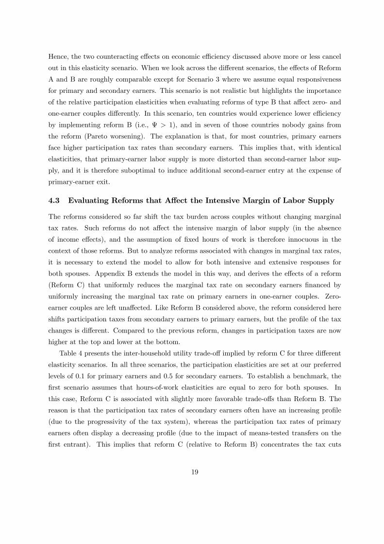
4.3 Evaluating Reforms that Affect the Intensive Margin of Labor Supply

The reforms considered so far shift the tax burden across couples without changing marginal

tax rates. Such reforms do not affect the intensive margin of labor supply (in the absence

of income effects), and the assumption of fixed hours of work is therefore innocuous in the

context of those reforms. But to analyze reforms associated with changes in marginal tax rates,

it is necessary to extend the model to allow for both intensive and extensive responses for

both spouses. Appendix B extends the model in this way, and derives the effects of a reform

(Reform C) that uniformly reduces the marginal tax rate on secondary earners financed by

uniformly increasing the marginal tax rate on primary earners in one-earner couples. Zero-

earner couples are left unaffected. Like Reform B considered above, the reform considered here

shifts participation taxes from secondary earners to primary earners, but the profile of the tax

changes is different. Compared to the previous reform, changes in participation taxes are now

higher at the top and lower at the bottom.

Table 4 presents the inter-household utility trade-off implied by reform C for three different

elasticity scenarios. In all three scenarios, the participation elasticities are set at our preferred

levels of 0.1 for primary earners and 0.5 for secondary earners. To establish a benchmark, the

first scenario assumes that hours-of-work elasticities are equal to zero for both spouses. In

this case, Reform C is associated with slightly more favorable trade-offs than Reform B. The

reason is that the participation tax rates of secondary earners often have an increasing profile

(due to the progressivity of the tax system), whereas the participation tax rates of primary

earners often display a decreasing profile (due to the impact of means-tested transfers on the

first entrant). This implies that reform C (relative to Reform B) concentrates the tax cuts

19

to secondary earners on those with the highest participation tax rates, while it concentrates

the tax increases for primary earners on those with the lowest participation tax rates. The

second scenario sets the intensive elasticity to 0.1 for both primary and secondary earners. This

generates an additional efficiency gain on the intensive margin for secondary earners, but also an

efficiency loss from the intensive responses of primary earners. The total effect is that trade-offs

are slightly more favorable. Scenario 3 features the same overall responsiveness on the intensive

margin as Scenario 2 (the sum of the two elasticities is unchanged), but the response is now

concentrated entirely on secondary earners. This makes reform C even more attractive and five

countries (Belgium, Denmark, France, Germany, and Sweden) can implement the reform at no

distributional cost.

Our conclusion is that the incorporation of hours-of-work responses into the analysis (assum-

ing realistic elasticities) does not change the qualitative insights offered above and has a fairly

small quantitative impact. If anything, the conclusions regarding the welfare effects of cutting

taxes for secondary earners are reinforced by this generalization.

5 Marriage Penalties in Europe

We now turn our attention to the tax-transfer implications of marriage. We present estimates

of the marriage penalty defined as the increase in the combined tax liability net of transfers of

two individuals following marriage.19 The marriage penalty has attracted significant interest

historically, especially in the United States where tax acts affecting married couples have often

been motivated by an attempt to ‘fix’ the problem of marriage penalties. The concern about

marriage penalties has been motivated by notions of fairness in the tax treatment of families

(horizontal equity across married and cohabitating couples), and by the possibility that tax and

transfer incentives distort the decision to marry. A number of papers have studied the effects

on marriage and divorce from income taxes (e.g., Alm and Whittington, 1995a,b, 1997, 1999),

welfare benefits (e.g., Hoynes, 1997a,b; Moffitt, 1998; Bitler et al., 2004), or taxes and benefits

combined (Dickert-Conlin, 1999; Eissa and Hoynes, 2000b). Although these studies tend to

find either modest or no effects, the implications of marriage disincentives continue to be a

controversial point of contention and marriage-dependent taxes and transfers are frequently

accused by conservatives of destroying the traditional two-parent family and creating higher

rates of single motherhood.

Almost all existing studies of marriage penalties focus on the United States and account

19While we use the term marriage penalty throughout the paper, it would perhaps be more precise to use thelabel formal cohabitation penalty. In principle, income transfers are based on family income regardless of maritalstatus, although in practice it is difficult for the authorities to verify cohabitation when there is no marriagecertificate.

20

only for the implications of the tax system (e.g., Rosen, 1987; Feenberg and Rosen, 1995; Alm

and Whittington, 1996; Dickert-Conlin and Houser, 1998; Bull et al., 1999; Alm et al., 1999;

Eissa and Hoynes, 2000a). An exception to this strong US-orientation in the literature is the

comparative study of marriage taxes by Pechman and Engelhardt (1990) who considered a subset

of the European countries in our sample. While Pechman and Engelhardt considered only the

tax system, we have seen in this paper that most of the jointness in redistribution schemes

in Europe is driven by the welfare system suggesting that there may be important transfer-

consequences to marriage. EUROMOD allows us to undertake a comparative study of marriage

penalties across a large set of countries, and to incorporate fully the implication of both the tax

and the transfer system.

It is helpful to start by considering some general properties of marriage penalties. Denoting

by T i (.) the tax function (net of transfers) that applies to individual filers and by T c (.) the tax

function applying to couples, the marriage penalty is defined as

MP ≡ T c (zp, zs)−£T i (zp) + T i (zs)

¤. (8)

Individual income tax treatment of couples, i.e. T c (zp, zs) = T i (zp)+T i (zs), is the only income

tax system that does not introduce a distortion of the marriage decision, MP = 0. On the other

hand, jointness generally implies MP 6= 0, and the sign of MP depends on the design of the

joint schedule and on the pair of incomes zp, zs in a given family. If MP is negative, we say

that there is a marriage subsidy. An example of a tax system giving rise to marriage subsidies

(ignoring the welfare system) is a progressive and fully joint tax scheme with income splitting,

so that each spouse is liable to pay taxes on half the couple’s combined earnings. Formally,

this is a system where T c (zp, zs) = T i³zp+zs2

´+ T i

³zp+zs2

´≡ T c (zp + zs). Income splitting

subsidizes marriage by allowing a couple to avoid part of the progressivity of the tax system.

Family-based and means-tested transfers generally give rise to marriage penalties. As in

Section 3, let us separate the T -functions into taxes (tc (.) , ti (.)) and benefits (bc (.) , bi (.)). The

combination of individual taxation and family-based transfers then implies MP ≡ bi (zp) +

bi (zs)− bc (zp + zs). Then, if the bi (.) and bc (.) functions are the same (so that marital status

is not an eligibility criterion in its own right), we have MP > 0 because b0 (.) < 0 as a result of

means-testing. Moreover, if there is additional targeting to single parents (in which case bc (z) <

bi (z) given the presence of children), the marriage penalty is even higher. Because family-based,

means-tested transfers as well as targeting to single motherhood tend to be very important at

the bottom of the distribution, we would expect to find significant marriage penalties at the

bottom. Moreover, these features would be particularly important in countries where welfare

systems are relatively generous (such as the Nordic countries).

21

The marriage penalty in eq. (8) is calculated using EUROMOD by measuring the change in

the combined tax liability net of transfers of a couple following a separation, holding individual

earnings constant.20 We consider households at ten different earnings configurations, ranging

from both spouses being out of work to both spouses earning at the top decile in their respective

earnings distributions, and we consider families with either two children or no children. When

children are involved, we assume that each spouse takes custody of one child after the divorce.21

We also assume that, following the divorce, each spouse faces half the rental cost of the couple

when they were married.22 The marriage penalties are shown in Table 5 for the case of two

children. Table A4 in the appendix shows the results for families without children. Marriage

penalties are reported on an annual basis and in 2007 Euros.

The results reveal substantial marriage penalties in most countries, and the penalties depend

primarily on the income of the lowest-earning spouse. Indeed, marriage penalties are often very

high even when the primary earner is at the top decile as long as second-earner income is low.

Moreover, marriage penalties are almost everywhere considerably higher when the couple has

children, often more than twice as high. These patterns point to the benefit system as an

important determinant of marriage penalties. In fact, in all countries, the strong targeting of

transfer programs to single parents is the single most important factor contributing to marriage

penalties. The tax system per se is not very important. As a result, the highest marriage

penalties are found in countries that have the most generous benefit programs such as the

Nordic countries, the Netherlands, France and Germany. Because of highly targeted transfers

to single parents, the United Kingdom and Ireland also show substantial marriage penalties for

families with children, although their social assistance programs are on the whole less generous

than those of the Nordic countries.

There are some exceptions to this general pattern of high marriage penalties. Italy offers

non-trivial marriage subsidies resulting from family benefits available only to married couples

with children. The tax-transfer system in Greece is virtually neutral with respect to marriage

for couples without children, but does feature minor penalties for couples with children. This

20Although individual earnings may of course change following a separation, it is conceptually important tokeep earnings constant in order to obtain the correct tax price on marriage. Notice that, if earnings were allowedto change at separation, even a fully individual-based redistribution scheme would appear to feature marriagepenalties or subsidies.21The assumption of a 1-1 split of custody is different from the usual assumptions in the (US-based) literature

on marriage taxes. This literature typically assumes that either (i) the children reside with the mother (Dickert-Conlin and Houser, 1998; Eissa and Hoynes, 2000a) or (ii) custody is determined by a tax minimization strategy(Rosen, 1987; Feenberg and Rosen, 1995). Because the second assumption implies that typically the higher-earnings spouse takes custody of all the children, whereas the first assumption implies that typically the lower-earnings spouse gets the kids, our assumption of an equal split lies in between these two extremes.22Our approach to the calculation of marriage penalties is closely related to the so-called “Resource Pooling

Approach” (see Bull et al., 1999). Our calculations do not include unearned income and therefore capture onlythe marriage penalty arising from the tax-transfer treatment of earned income.

22

is the result of an individual income tax combined with fairly small social assistance benefits

that are available only to single parents. Spain tends to subsidize marriage for couples without

children but penalize it for couples with children. In France, marriage subsidies are considerable

for higher-income families.23

6 Conclusion

The standard Mirrleesian theory of optimal income taxation assumes that all tax payers and

transfer recipients live in single-person households. In reality, most individuals live in families

formed around couples, and the tax-transfer rules applying to couples are often different from

the rules applying to single individuals. A number of recent papers have attempted to generalize

the theory of optimal income taxation to explicitly deal with couples. Instead of characterizing

the optimal tax-transfer treatment of families, this paper characterizes the actual tax-transfer

treatment of couples and identifies welfare-improving reforms for 15 European countries.

We have considered three aspects of a tax-transfer system for couples: the form of jointness,

the distortion of second-earner labor supply, and the size of marriage penalties. A general

insight from the analysis is that the transfer system is a crucial element in understanding and

evaluating redistribution schemes affecting married couples. For example, it is the presence of

family-based and means-tested transfer programs that explains the observation in many countries

of negative jointness, i.e. a negative relationship between the effective tax rate on one person and

the earnings of the spouse. Interestingly, negative jointness is in accordance with prescriptions

from the recent optimal tax literature (Kleven, Kreiner and Saez, 2007, 2008). At the same

time, family-based transfers tend to create substantial marriage penalties at the bottom of the

distribution, which raise issues pertaining to fairness and to some extent efficiency.

Our analysis of tax-transfer distortions at the extensive margin of labor supply suggests

that the effective taxation of secondary earners relative to primary earners is too high given

the empirical evidence on participation elasticities. Simple revenue-neutral reforms that shift

some of the tax burden from two-earner couples to one-earner and/or zero-earner couples would

reduce the distortion of second-earner labor supply and may generate substantial welfare gains.

In fact, for some countries, a tax cut for secondary earners may realistically pay for itself and

give rise to a Pareto improvement. For countries where Laffer effects are not present, a tax cut

for two-earner families does require a higher tax on other couples, but the required tax increase

23An additional important factor determining marriage penalties are housing benefits. In results not reportedhere, we have calculated marriage penalties under alternative assumptions about housing costs following separa-tion. For example, if rental costs for each spouse are at the same level as the combined rental costs of the couple(reflecting economies of scale in two-person households), the size of marriage penalties are considerably affectedin some countries (in particular, the UK, Ireland, Germany, Austria, Denmark, Finland, and the Netherlands).

23

tends to be reasonably small. In a majority of countries, it is possible to transfer 1 euro to

two-earner couples by taking away less than 12 a euro from other couples.

Appendix A: Derivation of eqs (6) and (7)

We derive the inter-household utility trade-off under the assumption that there are no households

with only the secondary earner working either before or after a reform. To ensure that this is

consistent with household optimization we must restrict the distribution of the fixed costs of

work for secondary earners. In terms of Figure 2, we must make sure that a marginal reform

does not induce any families to position themselves in area ∅. We denote by Vh (·) the indirectfamily utility function, which depends on the work status of the two spouses. The conditions we

will impose on the distribution of fixed costs of work for the secondary earner amount to saying

that, following a marginal reform, the indirect utility is greater for all families if they are in

area 0 of Figure 2 than if they are in area ∅. A sufficient condition makes sure that no coupleshave a high fixed cost of work for the primary earner qp and at the same time a relatively low

qs for the secondary earner.

Let q̄hs (0) ≡ Vh (0, 1)− V (0, 0) be the gain from secondary earner entry for household type

h when the primary earner is not working, and let q̄hp (1) ≡ Vh (1, 1) − Vh (0, 1) be the gain

from primary earner entry when the secondary earner is already working. Further, let qhp ≡min

©q̄hp (1) , q̄

hp

ªwhere q̄hp is determined by (4). We will assume a lower bound on the secondary

earner fixed costs of work depending on the primary earner’s fixed costs of work, qhs (qp), such

that Ph³qhs (qp) |qp

´≡ 0. The lower bound assumption is

qhs (qp) > qhs (0) for qp > qhp . (A-1)

The reason for the two different thresholds for the primary earner is that we must consider both

the potential movement from area 2 to area ∅ and from area 0 to area ∅ in Figure 2.With this assumption, there will be no households with only the secondary earner working

either before or after marginal reforms. Government revenue can then be written as

R =Xh

Nh

"Z q̄hp

0

Z q̄hs

qhs (qp)T³zhp , z

hs , θ´ph (qs |qp ) fh (qp) dqsdqp

+

Z q̄hp

0

Z ∞

q̄hs

T³zhp , 0, θ

´ph (qs |qp ) ph (qs |qp ) fh (qp) dqsdqp

+

Z ∞

q̄hp

Z ∞

qhs (qp)T (0, 0, θ) ph (qs |qp ) fh (qp) dqsdqp

#=

Xh

hT³zhp , z

hs , θ´Eh2 + T

³zhp , 0, θ

´Eh1 + T (0, 0, θ)Eh

0

i, (A-2)

24

where Eh2 is the number of two-earner households of type h, or equivalently, the number of

working secondary earners of type h, Eh1 is the number of one-earner households of type h, and

Eh0 is the number of type h households without any labor force attachment.

The effect of a small reform, dθ, on government revenue is given by

dR

dθ=

Xh

∙∂Th (1, 1)

∂θEh2 +

∂Th (1, 0)

∂θEh1 +

∂Th (0, 0)

∂θEh0

+Th (1, 1)dEh

2

dθ+ Th (1, 0)

dEh1

dθ+ Th (0, 0)

dEh0

dθ

¸=

Xh

∙∂Th (1, 1)

∂θEh2 +

∂Th (1, 0)

∂θEh1 +

∂Th (0, 0)

∂θEh0

+ [Th (1, 1)− Th (1, 0)]dEh

2

dθ+ [Th (1, 0)− Th (0, 0)]

µdEh

1

dθ+

dEh2

dθ

¶¸, (A-3)

becausedEh

0

dθ= −

µdEh

1

dθ+

dEh2

dθ

¶.

The first three terms in (A-3) reflect mechanical effects while the last two terms capture the

effects of the behavioral responses. The mechanical revenue effects are simply the direct effects

on tax revenue with unchanged behavior. The behavioral responses constitute new entry of

secondary earners (term 4) as well as new entry by primary earners (term 5).

The employment effects of the reform can be expressed using the participation elasticities

from the main text. The change in total employment among couples is

dEh1

dθ+

dEh2

dθ=

∂Eh1

∂q̄hp

dq̄hpdθ

= − ∂Eh1

∂zhp¡1− ahp

¢zhp ∂ahp∂θ= − 1

1− ahp

∂ahp∂θ

ηhpEh1 , (A-4)

where we have used∂ahp∂θ

=

µ∂Th (1, 0)

∂θ− ∂Th (0, 0)

∂θ

¶/zhp (0) . (A-5)

The change in secondary employment is

dEh2

dθ=

∂Eh2

∂q̄hs

dq̄hsdθ

= − ∂Eh2

∂zhs (1− ahs )zhs

∂ahs∂θ

= − 1

1− ahs

∂ahs∂θ

ηhsEh2 , (A-6)

where use is made of∂ahs∂θ

=

µ∂Th (1, 1)

∂θ− ∂Th (1, 0)

∂θ

¶/zhs (A-7)

Using (A-4) and (A-6) we can rewrite (A-3) as

dR

dθ=

Xh

∙∂Th (1, 1)

∂θEh2 +

∂Th (1, 0)

∂θEh1 +

∂Th (0, 0)

∂θEh0

¸

−Xh

"ahp

1− ahp

∂ahp∂θ

ηhpzhpE

h1 +

ahs1− ahs

∂ahs∂θ

ηhszhsE

h2

#.

25

Reform A. The first reform has

∂Th (1, 0)

∂θ=

∂Th (0, 0)

∂θ=

∂T (1, 0)

∂θ> 0,

∂Th (1, 1)

∂θ=

∂T (1, 1)

∂θ< 0 ∀h,

where the tax increase to one- and no-earner families is determined endogenously. Because the

reform is purely redistributive, government revenue must remain unchanged,dRdθ = 0, implying

−∂T (1, 0)∂θ

=

∂T (1,1)∂θ E2

³1−

PhEh2

E2

ahs1−ahs

ηhs

´N −E2

PhEh2

E2

³1− ahs

1−ahsηhs

´ ,

where E2 =P

hEh2 is the total number of two-earner households in the economy and where we

have used (A-7). From the envelope theorem and the marginal nature of the reform, monetary

gains and losses are simply the direct changes in tax liabilities. Because all two-earner couples

gain and all zero- and one-earner couples lose, we have

ΨA = −−P

h∂T (1,0)

∂θ

¡Nh −Eh

2

¢−P

h∂T (1,1)

∂θ Eh2

=−∂T (1,0)

∂θ (N −E2)∂T (1,1)

∂θ E2=(N −E2)

³1−

PhEh2

E2

ahs1−ahs

ηhs

´N −E2

PhEh2

E2

³1− ahs

1−ahsηhs

´ .

By inserting e2 ≡ E2/N and eh2 ≡ Eh2 /E2, we obtain expression (6).

Reform B. The second reform implies

∂Th (0, 0)

∂θ= 0,

∂Th (1, 0)

∂θ=

∂T (1, 0)

∂θ> 0,

∂Th (1, 1)

∂θ=

∂T (1, 1)

∂θ< 0 ∀h,

again with the tax increase for two-earner couples exogenously given. We find

−∂T (1, 0)∂θ

=

∂T (1,1)∂θ E2

³1−

PhEh2

E2

ahs1−ahs

ηhs

´E1

³1−

PhEh1

E1

ahp1−ahp

ηhp

´+P

hEh2

ahs1−ahs

ηhs

,

where E1 =P

hEh1 is the number of one-earner households and where we have used eqs (A-5)

and (A-7) as well as the fact that only primary earners in one-earner couples respond to the

reform. The trade-off between equity and efficiency equals ΨB = −−∂T (1,1)

∂θE2

−∂T (1,0)∂θ

E1. By inserting the

derivatives from above and the definitions e1 ≡ E1/N , eh1 = Eh1 /E1, e2 ≡ E2/N and eh2 ≡ Eh

2 /E2,

we obtain expression (7).

Appendix B: The intensive-extensive model

We introduce intensive responses by allowing individuals to choose working hours subject to

the costs of working time given by vp (zp/np) for primary earners and vs (zs/ns) for secondary

26

earners, where z/n is working time for an individual with earnings z and innate ability n. The

household utility function is now given by

u (c, zp, zs) = c− npvp

µzpnp

¶− nsvs

µzsns

¶− qp · 1 (zp > 0)− qs · 1 (zs > 0) .

Conditional on working, the primary earner chooses working hours according to

1−mhp (l) = v0p

Ãzhp (l)

nhp

!for l = 0, 1,

where mhp (·) ≡ T 0p is the marginal tax rate faced by the primary earner, which may depend

on the work status of the secondary earner. Thus, l = 1 denotes a working spouse and l = 0

represents a non-working secondary earner. Similarly, the number of working hours for the

secondary earners conditional on participation satisfies

1−mhs = v0s

µzhsnhs

¶,

where mhs ≡ T 0s denotes the marginal tax rate for the secondary earner (which does not depend

on the work status of the primary earner because a working secondary earner is always married

to a working primary earner). Household behavior along the intensive margin is captured by

the intensive elasticities

εhp (l) =1−mh

p (l)

zhp (l)

∂zhp (l)

∂£1−mh

p (l)¤ for l = 0, 1, εhs =

1−mhs

zhs

∂zhs∂(1−mh

s ),

which give the change in earnings in response to a change in the net-of-tax rate rates for the

primary and the secondary earner, respectively. Since the marginal tax rates of an individual

may now depend on spousal income, so may the choice of earnings. In particular, the earnings

of the primary earner are likely to change when the secondary earner enters the labor market.

Behavior along the extensive margin is governed by the exact same logic as in the simpler

model: the primary earner in household h enters whenever entry increases the family’s utility,

i.e., when Vh (1, 0)−V (0, 0) ≥ qp. Similarly, the secondary earner in household h enters whenever

Vh (1, 1)−Vh (1, 0) ≥ qs.24 Compared to the simpler model, the correct definition of the secondary

earner participation tax rate now includes the tax implications of the change in primary earnings,

i.e., ahs = T¡zhp (1) , z

hs , θ¢− T

¡zhp (0) , 0, θ

¢/zhs .

25

24Assumption (A-1) is again sufficient to solve the double screening problem.25 In the empirical simulations, we are forced to assume that primary earnings remain unchanged when the

secondary earner enters.

27

The definition of government revenue R is unchanged. The change in R as a result of the

reform, dθ, is

dR

dθ=

Xh

∙∂Th [1, 1]

∂θEh2 +

∂Th [1, 0]

∂θEh1 +

∂Th (0, 0)

∂θEh0

+ [Th (1, 1)− Th (1, 0)]dEh

2

dθ+ [Th (1, 0)− Th (0, 0)]

µdEh

1

dθ+

dEh2

dθ

¶+mh

p (1)dzhp (1)

dθEh2 +mh

s

dzhsdθ

Eh2 +mh

p (0)dzhp (0)

dθEh1

#. (A-8)

As before, the employment effects can be rewritten using elasticities to find

dR

dθ=

Xh

∙∂Th (1, 1)

∂θEh2 +

∂Th (1, 0)

∂θEh1 +

∂Th (0, 0)

∂θEh0

−ahp

1− ahp

∂ahp∂θ

ηhpzhp (0)E

h1 −

ahs1− ahs

∂ahs∂θ

ηhszhsE

h2

−mh

p (1)

1−mhp (1)

∂mhp (1)

∂θεhp (1) z

hp (1)E

h2

− mhs

1−mhs

∂mhs

∂θεhsz

hsE

h2

−mh

p (0)

1−mhp (0)

∂mhp (0)

∂θεhp (0) z

hp (0)E

h1

#.

Reform C. The details of the reform are

∂mhp (1)

∂θ=

∂Th (0, 0)

∂θ= 0,

∂mhp (0)

∂θ= τ =⇒ ∂Th (1, 0)

∂θ= τzhp (0) ,

∂mhs

∂θ= −t =⇒ ∂Th (1, 1)

∂θ= −tzhs ∀h,

where t > 0 is exogenous while τ is endogenously determined by government budget neutrality,

dR = 0. This implies

τ =tP

h zhsE

h2

³1− ahs

1−ahsηhs −

mhs

1−mhsεhs

´P

h zhp (0)E

h1

³1− ahp

1−ahpηhp +

Eh2

Eh1

ahs1−ahs

ηhs −mhp(0)

1−mhp(0)

εhp (0)´ .

Using this expression, the trade-off between equity and efficiency becomes

ΨC = −−P

h∂Th(1,0)

∂θ Ehp

−P

h∂Th(1,1)

∂θ Ehs

=τP

h zhp (0)E

h1

tP

h zhsE

h2

=1−

Ph s

hs

³ahs1−ahs

ηhs +mhs

1−mhsεhs

´1−

Ph s

hp

³ahp1−ahp

ηhp −eh2e2eh1e1

ahs1−ahs

ηhs +mhp (0)

1−mhp(0)

εhp (0)´ , (A-9)

28

where shp ≡ zhp (0)Ehp /¡P

h zhp (0)E

hp

¢is the share of all earnings in one-earner families that

accrues to households of type h, and shs ≡ zhsEhs /P

h zhsE

hs is the share of all secondary earnings

accruing to household h.

References

[1] Alesina, A. and A. Ichino (2007). “Gender based taxation.” Harvard University Working

Paper, April 2007.

[2] Alm, J. and L. Whittington (1995a). “Income Taxes and the Marriage Decision.” Applied

Economics 27, 25-31.

[3] Alm, J. and L. Whittington (1995b), “Does the Income Tax Affect Marital Decisions?”

National Tax Journal 48, 565-72.

[4] Alm, J. and L.A. Whittington (1996). “The Rise and Fall and Rise...of the Marriage Tax.”

National Tax Journal, 49, 571-89.

[5] Alm, J. and L.A. Whittington (1997). “Til Death or Taxes Do Us Part: The Effect of

Income Taxation on Divorce.” Journal of Human Resources 32, 388-412.

[6] Alm, J. and L.A. Whittington (1999). “For Love or Money? The Impact of Income Taxes

on Marriage.” Economica, 66, 571-89.

[7] Alm, J., S. Dickert-Conlin and L.A. Whittington (1999). “Policy Watch: The Marriage

Penalty.” Journal of Economic Perspectives, 13, 193-204.

[8] Armstrong, M. and J.-C. Rochet (1999). “Multi-dimensional screening: A user’s guide.”

European Economic Review, 43, 959-79.

[9] Bitler, M., J. Gelbach, H.W. Hoynes, and M. Zavodny (2004). “The Impact of Welfare

Reform on Marriage and Divorce.” Demography 41, 213-236.

[10] Blundell, R.W. (1995). “The Impact of Taxation on Labor Force Participation and Labor

Supply,” in OECD Job Study: Taxation, Employment, and Unemployment, Chapter 3,

OECD: Paris.

[11] Blundell, R.W. and T. MaCurdy (1999). “Labor Supply: A Review of Alternative Ap-

proaches.” In O. Ashenfelter and D. Card (eds.), Handbook of Labor Economics, Vol. 3A,

Amsterdam: Elsevier Science B.V., 1559-1695.

29

[12] Boskin, M. J.and E. Sheshinski (1983). “Optimal tax treatment of the family: Married

couples.” Journal of Public Economics, 20, 281-97.

[13] Brett, C. (2006). “Optimal Nonlinear Taxes for Families.” International Tax and Public

Finance 14, 225-261.

[14] Browning, E.K. and W.R. Johnson (1984). “The Trade-Off between Equality and Effi-

ciency.” Journal of Political Economy 92, 175-203

[15] Bull, N., J. Holtzblatt and J.R. Nunns (1999). “Defining and Measuring Marriage Penalties

and Bonuses.” OTA Paper 82.

[16] Cremer, Helmuth, Jean-Marie Lozachmeur, and Pierre Pestieau (2007). “Income Taxation

of Couples and the Tax Unit Choice.” Working Paper, 2007.

[17] Dickert-Conlin, S. (1999). “Taxes and Transfers: Their Effect on the Decision to End a

Marriage.” Journal of Public Economics 73, 217-40.

[18] Dickert-Conlin, S. and S. Houser (1998). “Taxes and Transfers: A New Look at the Marriage

Penalty.” National Tax Journal 51, 175-217.

[19] Eissa, N. (1995). “Taxation and Labor Supply of Married Women: The Tax Reform Act of

1986 as a Natural Experiment.” NBER Working Paper No. 5023.

[20] Eissa, N. and H.W. Hoynes (2000a). “Explaining the Fall and Rise in the Tax Cost of

Marriage: The Effect of Tax Laws and Demographic Trends, 1984-1997.” National Tax

Journal 53, 683-711.

[21] Eissa, N. and H.W. Hoynes (2000b). “Tax and Transfer Policy, and Family Formation:

Marriage and Cohabitation.” Working Paper, December 2000.

[22] Eissa. N. and H.W. Hoynes (2004). “Taxes and the Labor Market Participation of Married

Couples: The Earned Income Tax Credit.” Journal of Public Economics 88, 1931-1958.

[23] Eissa, N., H.J. Kleven, and Kreiner, C.T. “Evaluation of Four Tax Reforms in the United

States: Labor Supply and Welfare Effects for Single Mothers” Journal of Public Economics

92, 2008, 795-816.

[24] Feenberg, D. and H.S. Rosen (1995). “Recent Developments in the Marriage Tax.” National

Tax Journal 48, 91-101.

[25] Heckman, J. (1993). “What Has Been Learned About Labor Supply in the Past Twenty

Years?”, American Economic Review Papers and Proceedings, 83, 116-21.

30

[26] Hoynes, H.W. (1997a). “Does Welfare Play Any Role in Female Headship Decisions?” Jour-

nal of Public Economics 65, 89-117.

[27] Hoynes, H.W. (1997b). “Work, Welfare, and Family Structure: What Have We Learned?”,

in Fiscal Policy: Lessons From Economic Research, Alan Auerbach (ed.), MIT Press: Cam-

bridge, Massachusetts.

[28] Immervoll, H. (2004). “Average and marginal effective tax rates facing workers in the EU. A

micro-level analyis of levels, distributions and driving factors.” OECD Social, Employment

and Migration Working Paper No. 19, OECD: Paris.

[29] Immervoll, H. and C. O’Donoghue (2003). “Employment transitions in 13 European coun-

tries. Levels, distributions and determining Factors of net replacement rates.” CESifo Work-

ing Paper No. 1091, CESifo: Munich.

[30] Immervoll H., H.J Kleven, C.T. Kreiner and E. Saez (2007). “Welfare Reform in European

Countries: A Microsimulation Analysis.” Economic Journal, 117, 1-44.

[31] Kleven, H.J and C.T. Kreiner (2006). “The Efficient Taxation of Couples.” Mimeo.

[32] Kleven, H.J., C.T. Kreiner and E. Saez (2007). “The Optimal Income Taxation of Couples

as a Multi-Dimensional Screening Problem.” CESifo Working Paper 2092, September 2007.

[33] Kleven, H.J., C.T. Kreiner and E. Saez (2008). “The Optimal Income Taxation of Couples.”

Working Paper, August 2008. Forthcoming in Econometrica.

[34] Mirrlees, J.A. (1976). “Optimal tax theory: a synthesis.” Journal of Public Economics 6,

327-358.

[35] Mirrlees, James A. (1986). “The Theory of Optimal Taxation,” in K.J. Arrow and M.D.

Intrilligator (eds.), Handbook of Mathematical Economics vol. 3. Elsevier Science B.V.:

Amsterdam.

[36] Moffitt, R. (1998). “The Effect of Welfare on Marriage and the Family,” in Robert Moffitt

(ed.), Welfare and Family and Reproductive Behavior, National Academy Press: Washing-

ton D.C.

[37] OECD (2002). Revenue Statistics: 1965-2001. Paris: OECD.

[38] OECD (2003). National Accounts, Volume II 1990-2001. Paris: OECD.

[39] Pechman, J.A. (1987). Federal Tax Policy. Brookings Institution: Washington D.C.

31

[40] Pechman, J. and G. Engelhardt (1990). “The Income Tax Treatment of the Family: An

International Perspective.” National Tax Journal 43, 1-22.

[41] Rosen, H.S. (1977). “Is it time to abandon joint filing?” National Tax Journal, 30, 423-8.

[42] Rosen, H.S. (1987). “The Marriage Tax Is Down But Not Out.” National Tax Journal 40,

567-75.

[43] Rubenfeld, J. (1997). “Affirmative Action.” Yale Law Journal 107, 427-472.

[44] Saez E. (2002). “Optimal Income Transfer Programs: Intensive versus Extensive Labor

Supply Responses.” Quarterly Journal of Economics, 117, 1039-73.

[45] Schroyen, Fred (2003). “Redistributive taxation and the household: the case of individual

filings.” Journal of Public Economics 87, 2527-2547.

[46] Sutherland H. (2001). “Final Report EUROMOD: An Integrated European Benefit-Tax

Model.” EUROMOD Working Paper No. EM9/01.

32

Country One-earner couples

Two-earner couples

One- and two-earner couples

Austria 0.96 0.87 0.90Belgium 0.92 0.73 0.78Denmark 0.83 0.82 0.82Finland 0.65 0.76 0.75France 0.93 0.74 0.80Germany 0.91 0.78 0.83Greece 0.98 0.75 0.90Ireland 0.96 0.78 0.89Italy 0.94 0.81 0.88Luxembourg 0.99 0.77 0.89Netherlands 0.95 0.88 0.91Portugal 0.95 0.78 0.85Spain 0.97 0.73 0.89Sweden 0.66 0.76 0.75United Kingdom 0.78 0.83 0.81

Note: Secondary earners are defined as the spouses with the lowest earnings in the couples. Source: EUROMOD Microsimulation Model.

Table 1. Share of women among secondary earners

Participation Tax Participation Tax Relative Tax Relative Participation Relative EarningsCountry Primary Earners Secondary Earners (PE / SE) ( PE / SE ) ( PE / SE )Austria 0.63 0.36 1.72 1.66 2.18Belgium 0.73 0.74 0.98 1.38 1.95Denmark 0.73 0.53 1.38 1.13 1.74Finland 0.60 0.36 1.65 1.05 1.66France 0.85 0.63 1.35 1.53 1.67Germany 0.63 0.51 1.22 1.53 1.99Greece 0.27 0.28 0.97 3.13 1.61Ireland 0.54 0.44 1.22 2.55 2.18Italy 0.35 0.46 0.77 2.15 1.51Luxembourg 0.50 0.32 1.54 2.52 2.25Netherlands 0.56 0.44 1.28 1.68 2.61Portugal 0.37 0.41 0.90 1.74 1.56Spain 0.34 0.41 0.83 3.25 1.61Sweden 0.66 0.51 1.28 1.07 1.53United Kingdom 0.56 0.20 2.79 1.47 2.20

Note: The first two columns list the average effective participation tax rates for primary earners in one-earner couples and secondary earners in two-earner families, respectively. Colums 4 shows relative participation rates of primary and secondary earners and column 5 lists the relative average earnings of primary and secondary earners conditional on working. The calculation of the tax rates is descibed in the text. Source: EUROMOD Microsimulation Model.

Table 2. Participation tax rates and labor market outcomes

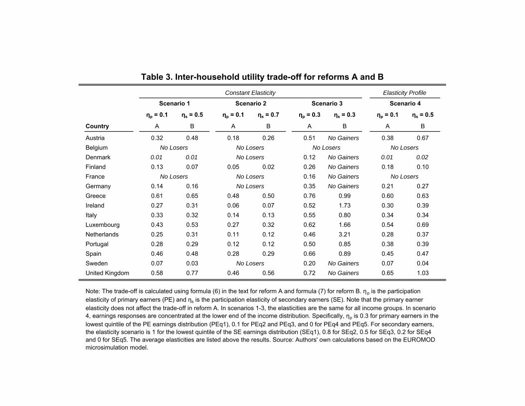
ηp = 0.1 ηs = 0.5 ηp = 0.1 ηs = 0.7 ηp = 0.3 ηs = 0.3 ηp = 0.1 ηs = 0.5

Country A B A B A B A B

Austria 0.32 0.48 0.18 0.26 0.51 No Gainers 0.38 0.67BelgiumDenmark 0.01 0.01 0.12 No Gainers 0.01 0.02Finland 0.13 0.07 0.05 0.02 0.26 No Gainers 0.18 0.10France 0.16 No GainersGermany 0.14 0.16 0.35 No Gainers 0.21 0.27Greece 0.61 0.65 0.48 0.50 0.76 0.99 0.60 0.63Ireland 0.27 0.31 0.06 0.07 0.52 1.73 0.30 0.39Italy 0.33 0.32 0.14 0.13 0.55 0.80 0.34 0.34Luxembourg 0.43 0.53 0.27 0.32 0.62 1.66 0.54 0.69Netherlands 0.25 0.31 0.11 0.12 0.46 3.21 0.28 0.37Portugal 0.28 0.29 0.12 0.12 0.50 0.85 0.38 0.39Spain 0.46 0.48 0.28 0.29 0.66 0.89 0.45 0.47Sweden 0.07 0.03 0.20 No Gainers 0.07 0.04United Kingdom 0.58 0.77 0.46 0.56 0.72 No Gainers 0.65 1.03

No Losers No Losers

Note: The trade-off is calculated using formula (6) in the text for reform A and formula (7) for reform B. ηp is the participation elasticity of primary earners (PE) and ηs is the participation elasticity of secondary earners (SE). Note that the primary earner elasticity does not affect the trade-off in reform A. In scenarios 1-3, the elasticities are the same for all income groups. In scenario 4, earnings responses are concentrated at the lower end of the income distribution. Specifically, ηp is 0.3 for primary earners in the lowest quintile of the PE earnings distribution (PEq1), 0.1 for PEq2 and PEq3, and 0 for PEq4 and PEq5. For secondary earners, the elasticity scenario is 1 for the lowest quintile of the SE earnings distribution (SEq1), 0.8 for SEq2, 0.5 for SEq3, 0.2 for SEq4 and 0 for SEq5. The average elasticities are listed above the results. Source: Authors' own calculations based on the EUROMOD microsimulation model.

No Losers

No Losers

Table 3. Inter-household utility trade-off for reforms A and B

Scenario 1

No Losers No Losers

Scenario 4

No Losers

No Losers No Losers

No Losers

Scenario 3

Elasticity ProfileConstant Elasticity

Scenario 2

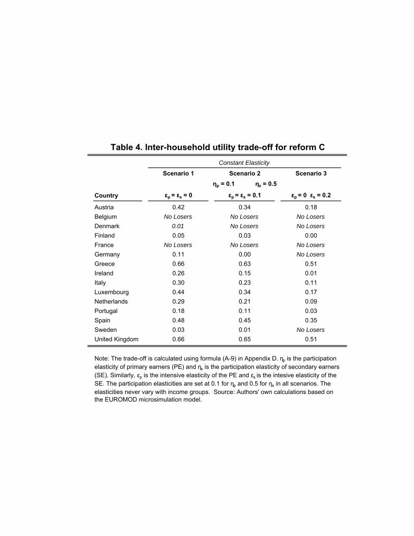
Scenario 1 Scenario 2 Scenario 3

Country εp = εs = 0 εp = εs = 0.1 εp = 0 εs = 0.2

Austria 0.42 0.34 0.18Belgium No Losers No Losers No LosersDenmark 0.01 No Losers No LosersFinland 0.05 0.03 0.00France No Losers No Losers No LosersGermany 0.11 0.00 No LosersGreece 0.66 0.63 0.51Ireland 0.26 0.15 0.01Italy 0.30 0.23 0.11Luxembourg 0.44 0.34 0.17Netherlands 0.29 0.21 0.09Portugal 0.18 0.11 0.03Spain 0.48 0.45 0.35Sweden 0.03 0.01 No LosersUnited Kingdom 0.66 0.65 0.51

ηp = 0.1 ηs = 0.5

Constant Elasticity

Table 4. Inter-household utility trade-off for reform C

Note: The trade-off is calculated using formula (A-9) in Appendix D. ηp is the participation elasticity of primary earners (PE) and ηs is the participation elasticity of secondary earners (SE). Similarly, εp is the intensive elasticity of the PE and εs is the intesive elasticity of the SE. The participation elasticities are set at 0.1 for ηp and 0.5 for ηs in all scenarios. The elasticities never vary with income groups. Source: Authors' own calculations based on the EUROMOD microsimulation model.

Family Income Percentiles AT BE DK FI FR GE GR IR IT LU NL PT SP SW UK

PE 0 - SE 0 5141 9770 7077 3676 14472 2387 1608 2224 0 7433 13549 0 0 10187 4696

PEp10 - SE 0 9353 10090 11640 6668 13059 5138 619 9156 -3234 12474 13375 2276 69 10495 7586

PEp10 - SEp10 7167 9712 11153 5116 7343 6573 762 10711 -1025 10624 11762 1125 837 5987 7782

PEp50 - SE 0 9353 6933 18148 12114 12096 9040 518 9999 -2307 10288 13632 2151 7 17444 13234

PEp50 - SEp10 7178 7071 11858 5611 6433 7692 615 7831 -686 4672 12343 593 849 5730 9406

PEp50 - SE p50 496 -575 9411 1055 2404 2267 57 3561 256 -3169 8814 355 1669 752 6066

PEp90 - SE 0 9353 6101 21936 14040 7308 8173 588 14318 -935 3249 12195 -187 7 17987 20780

PEp90 - SEp10 7294 6110 13457 7691 1962 7182 686 13868 -158 -2967 10713 -1621 1809 5730 17130

PEp90 - SEp50 496 -1274 10060 1055 -1192 3027 73 7023 294 -8042 6663 -1156 2821 1938 13790

PEp90 - SEp90 697 -575 6259 737 -288 955 244 5839 -422 -1027 7942 651 3316 0 2108

Note: The table shows marriage penalties on an annual basis for hypothetical families in 2007 Euros. The calculations are done for different earnings levels for the primary and secondary earner and the earnings levels refer to percentiles in the earnings distribution for primary and secondary earners, respectively. The marriage penalty is calculated as the change in a couple's combined (net-)tax liability upon separation. It is assumed that all individuals occupy rental housing. Following separation, each spouse is assumed to bear rental costs amounting to 50% of the costs in the married scenario. Further, each spouse retains custody of one child. 1998 figures are converted to 2007 euros using national indices of compensation per employee. Exchange rates are, respectively, the irrevocable euro exchange rates (12 euro countries) and 2007 average annual exchange rates (non-euro countries: Denmark, Sweden, UK). Sources: EUROMOD microsimulation model, OECD Economic Outlook 82, and Danmarks Nationalbank.

Table 5. Annual marriage penalties in 2007 euros for families with two children, 1998

Figure 1. Participation tax rates of secondary earners (in percent) at selected earnings levels as a function of primary earnings (vingtiles) for couples with two children

0

100

1 2 3 4 5 6 7 8 9 10 11 12 13 14 15 16 17 18 19 20bottom 5% bottom 10% median top 10%

102030405060708090

100110

Denmark

102030405060708090

100110

Austria

102030405060708090

100110

Belgium

Figure continues on the next page

010

1 2 3 4 5 6 7 8 9 10 11 12 13 14 15 16 17 18 19 20

0102030405060708090

100110

1 2 3 4 5 6 7 8 9 10 11 12 13 14 15 16 17 18 19 20

Finland

0102030405060708090

100110

1 2 3 4 5 6 7 8 9 10 11 12 13 14 15 16 17 18 19 20

France

0102030405060708090

100110

1 2 3 4 5 6 7 8 9 10 11 12 13 14 15 16 17 18 19 20

Germany

010

1 2 3 4 5 6 7 8 9 10 11 12 13 14 15 16 17 18 19 20

010

1 2 3 4 5 6 7 8 9 10 11 12 13 14 15 16 17 18 19 20

Figure 1 cont.0

100

1 2 3 4 5 6 7 8 9 10 11 12 13 14 15 16 17 18 19 20bottom 5% bottom 10% median top 10%

8090

100110

Luxembourg

8090

100110

Netherlands

8090

100110

Portugal

Greece

0102030405060708090100110

1 2 3 4 5 6 7 8 9 10 11 12 13 14 15 16 17 18 19 20

Ireland

0102030405060708090100110

1 2 3 4 5 6 7 8 9 10 11 12 13 14 15 16 17 18 19 20

Italy

0102030405060708090100110

1 2 3 4 5 6 7 8 9 10 11 12 13 14 15 16 17 18 19 20

Note: Each figure shows the participation tax rate of the secondary earner (SE) in percent as a function of the earnings of the primary earner (PE), depicted by vingtile group in the PE earnings distribution. The graphs are shown for four different SE earnings levels: the lowest vingtile (SEp5), the lowest decile (SEp10), the median(SEp50), and the top decile (SEp90) of the SE earnings distribution. Source: EUROMOD microsimulation model.

010203040506070

1 2 3 4 5 6 7 8 9 10 11 12 13 14 15 16 17 18 19 200

10203040506070

1 2 3 4 5 6 7 8 9 10 11 12 13 14 15 16 17 18 19 200

10203040506070

1 2 3 4 5 6 7 8 9 10 11 12 13 14 15 16 17 18 19 20

0102030405060708090

100110

1 2 3 4 5 6 7 8 9 10 11 12 13 14 15 16 17 18 19 20

Spain

0102030405060708090

100110

1 2 3 4 5 6 7 8 9 10 11 12 13 14 15 16 17 18 19 20

Sweden

0102030405060708090

100110

1 2 3 4 5 6 7 8 9 10 11 12 13 14 15 16 17 18 19 20

UK

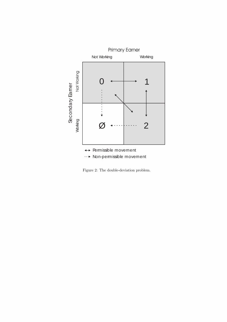
Not Working

Wor

king

Working

Seco

ndar

y Ea

rner 0 1

Ø 2

Permissible movementNon-permissible movement

Figure 2: The double-deviation problem.

Table A1: Summary of taxes on workers

Income Tax7 SSC (employee) SSC (employer) and Payroll Tax

lowest/highest tax band limit1,2

lowest/highest rate [%] main tax credit1 tax unit family-related tax provisions

thres-hold1 rate [%] ceiling1 tax

deductiblethres-hold1 rate [%] ceiling1 taxable

Austria 17/231 21/504 rates 5 individual deduction for single earners;

tax credits for lone parents 15 18.8 193 yes 15-

21.34.5

193- no 2nd earner: phase-out of single-earner

credit

Belgium 24/318 25/557 rates - individual

parts of taxable income transferrable to spouse;

additional tfa for children and lone parents

- 11.9 - yes - 45.4 - no2nd earner: phase-out of amount transferrable from higher-earning

spouse

Denmark 12/100 40/594

3 rates- individual unused deductions

transferrable to spouse - 9+ flat amount - yes - 2

+ flat amount - no

Finland 35/223 24/564

6 rates- individual -

587.60.5 - yes - 24.5 - no earned income tax allowance (20% of

earnings above 11)

phase-out of earned income tax and basic allowances (starting at earnings >

31 and 76 respectively)

France 30/336 11/546 rates - family

---

136-

0.99.62.84

3.67.6

-136409545

-

yesyesyesyes

partly

---

136

19.813.44.15.3

-136409545

no reduced employer contributions rates for wages < 130% MW.

Germany30

133252

27.337.255.75

-

married couple

(individual optional)

choice of tfa or child benefit 15 7.713.4

156208 yes 15 7.7

13.4156208 no

Greece 56/478 5/455 rates

max. 15% of accepted hshld.

expenditureindividual 0.9-1.8 non-refundable tax

credit per child - 15.9200;

none for new jobs

yes - 28.2200;

none for new jobs

no

Ireland 25/80 24/462 rates -

married couple

(individual optional)

- 4186

4.52.3

193- no

-112

-

8.512.04.0

12231231

no no tax if income below 33 (higher limit if children)

tax-free status phased out above the 33 limit.

Italy 0/118 19/465 rates up to 6 individual up to 2 tax credit for each

dependent family member-

569.04

1- yes - 33.04 - no

phase-out of main tax credit;2nd earner: phase-out of tax credit for

dependent spouse;

Luxembourg 25/250 6/4717 rates - married

couple

deductions for lone parents and care expenditure; 3 tax

credit per child- 13.1 259 yes - 14.64 259 no 2nd earner: additional tax deduction if

both spouses work

Netherlands 20/212 368/603 rates

- individual additional tfa for lone parents

54-

5.31.7

156105

yesno

54--

6.45.67.94

156105156

noyesno

Portugal 0/490 59/405 rates

3 married couple

additional 1.5 tax credit per child - 11 - no - 23.8 - no

Spain 22/492 20/568 rates 3

family (individual optional)

up to 2 tax credit per child (additional amounts in some

regions)46 30.8 177 yes 46 6.4 177 no earning < 55 are tax-exempt

"spike" in METR once above exemption limit; phase-out of main tax

credit adds 5 pct. points to METR

Sweden 4/92 304

554 - individual - 3 6.95 121 yes 0.4 33 - no

United Kindgom

29/220 20/403 rates - individual

2 tax credit for married couples; 13 tax deduction for

lone parents23 8.4 to 10 177 no

2310

405676

357

10

- no

features increasing METR and PTRfeatures reducing METR and PTR

Appreviations: SSC = social security contribution; METR = marginal effective tax rate; PTR = participation tax rate; tfa = tax free allowance; MW = statutory minimum wage.

10 all earnings are subject to the applicable rate once they exceed these threshold levels

Explanatory Notes: Reference year is 1998. Except where noted, all information is for private-sector employees with no other income and not claiming itemised expenses. Income taxes include local and regional taxes where applicable. Multiple lines of SSC entries are shown where payment schedules differ for the different programs (e.g. for pensions, health, unemployment, etc.). Further information, and data for later years, can be found in the EUROMOD country reports (www.iser.essex.ac.uk/msu/emod/documentation/countries/), the OECD Tax Database (www.oecd.org/ctp/taxdatabase) and the OECD series Benefits and Wages ( www.oecd.org/els/social/workincentives) .

6 West Germany7 including regional income taxes where applicable8 including pension contributions (same tax base as income tax)9 effective rate taking into account the allowance of 70% of the tax base for low incomes

1 in % of median gross earnings of primary earners (not including employer social security contributions)2 after adding any standard tax free allowances, deductions or exemptions available to single employees3 insurance is voluntary4 averages: rates differ between municipalities and/or employers5 including "Solidarity Surplus Tax" for German unification. MTR increases linearly inbetween lower and middle; and middle and top tax band limits.

Table A2: Summary of social benefits available to persons of working-ageSocial Assistance Housing Benefit2 Family Benefits3 Employment-conditional Benefits

max. amount1 disregard1 withdrawal rate taxable max. amount1 withdrawal rate amount1 withdrawal rate amount1 work/income conditions withdrawal rate

Austria 52 - 100% IT: noSSC: no - - 5-7 per child none

(universal payment) - - -

Belgium 53 10 for each working adult 100% IT: no

SSC: no - - 4-13 per child none(universal payment) - - -

Denmark90

+ housing allowance

9 for each working adult 100% IT: yes

SSC: no 11 75% 3-4 per child; higher for lone parents

none(universal payment) - - -

Finland58

+reasonable housing cost

- 100% IT: noSSC: no 34 80%

5-9 per child; plus 2 per child for lone parents; plus

day-care subsidy

none(universal payment) - - -

France 49 - 100% IT: noSSC: no 20 34%

main benefit: 7 to 12 for second & further children; special benefits for young

children

main benefit: 100% once income > 174-261 - - -

Germany474

+ reasonable housing costs

4 for each working family

member

75-100% IT: noSSC: no

45(if not receiving

social assistance)40%

main benefit: 5-9 per child; child-raising allowance for

very young children: additional 5-7

main benefit: none (universal payment);

child-raising allowance: 20-40% once income > 62

- - -

Greece - - - - 0.5-1 per child plus additions for large families

reduced in steps for incomes > 65 - - -

Ireland 5619

(only for 2nd earner)

100% IT: noSSC: no 53 100% 3-4 per child none

(universal payment)

60% of family gross earnings exceeding 88 (higher limit for

larger families)

couple jointly working at least 20 hours per week

60% (of gross family earnings)

Italy - - - -3-17 per family member (also spouses) depending on family

type

must work at least 3 days per week; reduced

benefits if working less than full-time

reduced in steps for family incomes > 73

Luxembourg 64 13 100% IT: yesSSC: reduced

6(must receive social

assistance)100%

8-13 per child; plus education allowance for

children aged 3-

none(universal payment) - - -

Netherlands 49 - 100%

yes, but max. amount is

shown on net basis

6 54% 2-7 per child none(universal payment) - - -

Portugal 59 - 100% IT: noSSC: no 4 per child reduced to 3 per child once

income > 71 - - -

Spain 2 for first child, 0.2 for further children 100% once income > 55 - - -

Sweden35

+reasonable housing cost

- 100% IT: noSSC: no 17 33%

(disregard of 18) 4-8 per child none(universal payment) - - -

United Kindgom 51 2-4 100% IT: noSSC: no

100% of recognised rent; 100% of council

tax

65% (housing benefit); 20% (council tax

benefit)3-5 per child none

(universal payment)

18 + up to 13 per child + 4 if working > 30 hours per week;

only entitled if >= 1 child

at least one person working >= 16 hours per

week

70% of family income > 29

1 in % of median gross earnings of primary earners (not including employer social security contributions)2 cash assistance for privately rented accommodation. Housing benefits may be paid through the social assistance program. In this case, they are already reflected in the social assistance amounts shown in this table.

Abbreviations: IT = income tax; SSC = social security contributions.

4 West Germany

3 in addition to family-related tax concessions shown in the companion table under income tax. Does not include any benefits available for pregnancy, childbirth, parental leave, or childcare benefits.

none at the national level

none at the national level

Explanatory Notes: Reference year is 1998. Rules for social benefits can vary between regions or municipalities. Where social assistance is subject to job-search or other conditions (e.g. in Denmark), it is assumed that both spouses comply with the relevant requirements. All information is for families with two children. IT = income tax; SSC = social security contributions. Further information, and data for later years, can be found in the EUROMOD country reports (www.iser.essex.ac.uk/msu/emod/documentation/countries/ ), the OECD Tax Database (www.oecd.org/ctp/taxdatabase ) and the OECD series Benefits and Wages ( www.oecd.org/els/social/workincentives) .

none at the national level none at the national level

see employment-conditional benefits

none at the national level

Country Primary earners Secondary earners PE tax / SE taxAustria 0.52 0.44 1.19Belgium 0.65 0.60 1.08Denmark 0.58 0.54 1.07Finland 0.54 0.47 1.16France 0.53 0.53 0.99Germany 0.54 0.59 0.92Greece 0.37 0.28 1.32Ireland 0.43 0.43 1.01Italy 0.52 0.48 1.07Luxembourg 0.41 0.44 0.95Netherlands 0.52 0.47 1.12Portugal 0.44 0.42 1.03Spain 0.37 0.32 1.17Sweden 0.59 0.54 1.09United Kingdom 0.37 0.31 1.21

Note: Average effective marginal tax rates for primary earners and secondary earners conditional on working. Source: EUROMOD Microsimulation Model.

Table A3. Average marginal tax rates

Family Income Percentiles AT BE DK FI FR GE GR IR IT LU NL PT SP SW UK

PE 0 - SE 0 4905 5217 -2990 2066 5907 760 0 2224 0 8110 2443 0 0 10384 2418

PEp10 - SE 0 7510 5319 4966 7263 7306 4008 -24 7069 -1527 13281 6312 1652 -421 14126 4994

PEp10 - SEp10 4875 5684 199 2214 2440 2587 -24 4471 -437 8298 5385 94 0 2251 3336

PEp50 - SE 0 7780 5861 8184 8340 6915 3273 -145 5078 -957 9089 6190 1241 -969 14508 8075

PEp50 - SEp10 5228 6741 264 2224 1485 1913 -145 1235 -456 3201 4886 -317 -127 2251 3587

PEp50 - SE p50 0 1655 0 0 -170 -149 11 -1507 -625 -3827 961 142 0 0 -609

PEp90 - SE 0 8020 6027 8985 9621 1092 -356 0 5922 -1619 3121 8937 -999 -2122 14508 13411

PEp90 - SEp10 5969 6779 1031 3223 -3263 -1468 0 2698 -1207 -3539 7560 -2434 -320 2251 9049

PEp90 - SEp50 0 1954 1464 0 -3262 -5517 106 -1212 -1377 -7801 0 -1169 0 0 3148

PEp90 - SEp90 0 3077 0 0 -1251 -1682 287 0 -1677 -3662 0 638 0 0 -610

Note: The table shows marriage penalties on an annual basis for hypothetical families in 2007 Euros. The calculations are done for different earnings levels for the primary and secondary earner and the earnings levels refer to percentiles in the earnings distribution for primary and secondary earners, respectively. The marriage penalty is calculated as the change in a couple's combined (net-)tax liability upon separation. It is assumed that all individuals occupy rental housing. Following separation, each spouse is assumed to bear rental costs amounting to 50% of the costs in the married scenario. Further, each spouse retains custody of one child. 1998 figures are converted to 2007 euros using national indices of compensation per employee. Exchange rates are, respectively, the irrevocable euro exchange rates (12 euro countries) and 2007 average annual exchange rates (non-euro countries: Denmark, Sweden, UK). Sources: EUROMOD microsimulation model, OECD Economic Outlook 82, and Danmarks Nationalbank.

Table A4. Annual marriage penalties in 2007 euros for families with no children, 1998

Figure A1. Marginal tax rates of secondary earners (in percent) at selected earnings levels as a function of primary earnings (vingtiles) for couples with two children

30405060708090

100110

Belgium

30405060708090

100110

Austria

0

100

1 2 3 4 5 6 7 8 9 10 11 12 13 14 15 16 17 18 19 20bottom 5% bottom 10% median top 10%

30405060708090

100110

Denmark

Figure continues on the next page

01020

1 2 3 4 5 6 7 8 9 10 11 12 13 14 15 16 17 18 19 20

01020

1 2 3 4 5 6 7 8 9 10 11 12 13 14 15 16 17 18 19 20

01020

1 2 3 4 5 6 7 8 9 10 11 12 13 14 15 16 17 18 19 20

0102030405060708090

100110

1 2 3 4 5 6 7 8 9 10 11 12 13 14 15 16 17 18 19 20

Finland

0102030405060708090

100110

1 2 3 4 5 6 7 8 9 10 11 12 13 14 15 16 17 18 19 20

France

0102030405060708090

100110

1 2 3 4 5 6 7 8 9 10 11 12 13 14 15 16 17 18 19 20

Germany

Figure A1 cont.0

100

1 2 3 4 5 6 7 8 9 10 11 12 13 14 15 16 17 18 19 20bottom 5% bottom 10% median top 10%

8090

100110

Luxembourg

8090

100110

Netherlands

8090

100110

Portugal

Greece

0102030405060708090

100110

1 2 3 4 5 6 7 8 9 10 11 12 13 14 15 16 17 18 19 20

Ireland

0102030405060708090

100110

1 2 3 4 5 6 7 8 9 10 11 12 13 14 15 16 17 18 19 20

Italy

01020304050

60708090100110

1 2 3 4 5 6 7 8 9 10 11 12 13 14 15 16 17 18 19 20

Note: Each figure shows the marginal tax rate of the secondary earner (SE) in percent as a function of the earnings of the primary earner (PE), depicted by vingtile group in the PE earnings distribution. The graphs are shown for four different SE earnings levels: the lowest vingtile (SEp5), the lowest decile (SEp10), the median(SEp50), and the top decile (SEp90) of the SE earnings distribution. Source: EUROMOD microsimulation model.

01020304050607080

1 2 3 4 5 6 7 8 9 10 11 12 13 14 15 16 17 18 19 20

01020304050607080

1 2 3 4 5 6 7 8 9 10 11 12 13 14 15 16 17 18 19 20

010203040506070

1 2 3 4 5 6 7 8 9 10 11 12 13 14 15 16 17 18 19 20

0102030405060708090

100110

1 2 3 4 5 6 7 8 9 10 11 12 13 14 15 16 17 18 19 20

Spain

0102030405060708090

100110

1 2 3 4 5 6 7 8 9 10 11 12 13 14 15 16 17 18 19 20

Sweden

0102030405060708090

100110

1 2 3 4 5 6 7 8 9 10 11 12 13 14 15 16 17 18 19 20

UK

Figure A2. Participation tax rates of secondary earners (in percent) at selected earnings levels as a function of primary earnings (vingtiles) for couples with no children

0

100

1 2 3 4 5 6 7 8 9 10 11 12 13 14 15 16 17 18 19 20

bottom 5% bottom 10% median top 10%

405060708090

100110

Denmark

405060708090

100110

Austria

405060708090

100110

Belgium

Figure continues on the next page

0102030

1 2 3 4 5 6 7 8 9 10 11 12 13 14 15 16 17 18 19 20

0102030405060708090

100110

1 2 3 4 5 6 7 8 9 10 11 12 13 14 15 16 17 18 19 20

Finland

0102030405060708090

100110

1 2 3 4 5 6 7 8 9 10 11 12 13 14 15 16 17 18 19 20

France

0102030405060708090

100110

1 2 3 4 5 6 7 8 9 10 11 12 13 14 15 16 17 18 19 20

Germany

0102030

1 2 3 4 5 6 7 8 9 10 11 12 13 14 15 16 17 18 19 20

0102030

1 2 3 4 5 6 7 8 9 10 11 12 13 14 15 16 17 18 19 20

Figure A2 cont.

0

100

1 2 3 4 5 6 7 8 9 10 11 12 13 14 15 16 17 18 19 20bottom 5% bottom 10% median top 10%

8090

100110

Luxembourg

8090

100110

Netherlands

8090

100110

Portugal

Greece

0102030405060708090100110

1 2 3 4 5 6 7 8 9 10 11 12 13 14 15 16 17 18 19 20

Ireland

0102030405060708090100110

1 2 3 4 5 6 7 8 9 10 11 12 13 14 15 16 17 18 19 20

Italy

01020304050

60708090100110

1 2 3 4 5 6 7 8 9 10 11 12 13 14 15 16 17 18 19 20

Note: Each figure shows the participation tax rate of the SE in percent as a function of the earnings of the PE, depicted by vingtile group in the PE earnings distribution. The graphs are shown for four different SE earnings levels: the lowest vingtile (SEp5), the lowest decile (SEp10), the median(SEp50), and the top decile (SEp90) of the SE earnings distribution. Source: EUROMOD microsimulation model.

01020304050607080

1 2 3 4 5 6 7 8 9 10 11 12 13 14 15 16 17 18 19 20

010203040506070

1 2 3 4 5 6 7 8 9 10 11 12 13 14 15 16 17 18 19 200

1020304050607080

1 2 3 4 5 6 7 8 9 10 11 12 13 14 15 16 17 18 19 20

0102030405060708090

100110

1 2 3 4 5 6 7 8 9 10 11 12 13 14 15 16 17 18 19 20

Spain

0102030405060708090

100110

1 2 3 4 5 6 7 8 9 10 11 12 13 14 15 16 17 18 19 20

Sweden

0102030405060708090

100110

1 2 3 4 5 6 7 8 9 10 11 12 13 14 15 16 17 18 19 20

UK