Discrete choice modelling of labour supply in Luxembourg through EUROMOD microsimulation

EUROMOD

WORKING PAPER SERIES

EUROMOD Working Paper No. EM5/10

DISCRETE CHOICE MODELLING OF LABOUR SUPPLY IN LUXEMBOURG THROUGH

EUROMOD MICROSIMULATION

Frédéric Berger, Nizamul Islam, Philippe Liégeois

August 2010

DISCRETE CHOICE MODELLING OF LABOUR SUPPLY IN LUXEM BOURG THROUGH EUROMOD MICROSIMULATION 1

Frédéric Berger, Nizamul Islam, Philippe Liégeois2

Abstract

In this study, the household labour supply is modelled as a discrete choice problem assuming that preference for leisure and consumption can be described by a quadratic utility function which allows for non-convexities in the budget set. We assess behavioural responses to the significant changes in the tax-benefit system during 2001-2002 in Luxembourg. Only moderate impact is found, on average, on the efficiency of the economy as measured by the labour supply effects. The impact is indeed concentrated on richer single women. These increase significantly their labour force, which more than doubles the non-behavioural effect of the tax reform on disposable income and boosts the gains in well-being for that part of population.

JEL Classification: C25, H24, H31, J22

Keywords: Labour supply, Discrete choice, Households, EUROMOD, Microsimulation, Tax reform

Corresponding author: Nizamul Islam CEPS/INSTEAD 44, rue Emile Mark L-4620 Differdange Grand-Duchy of Luxembourg E-mail: [email protected]

1 This paper uses EUROMOD version 31A and data from the PSELL/EU-SILC for 2004 (income 2003) made available by CEPS/INSTEAD. EUROMOD is continually being improved and updated and the results presented here represent the best available at the time of writing. 2 The paper was written as part of the REDIS project (“Coherence of Social Transfer Policies in Luxembourg through the use of microsimulation models”), financed by the Luxembourg National Research Fund under Grant FNR/06/28/19. We are indebted to all past and current members of the EUROMOD consortium for the construction and development of EUROMOD. We also wish to thank Raymond Wagener from the Inspection Générale de la Sécurité Sociale in Luxembourg for continuous support. However, any remaining errors, results produced, interpretations or views presented in the paper are the authors' responsibility. In particular, the paper does not represent the views of the institutions to which the authors are affiliated.

1. INTRODUCTION

In all countries, the influence of governmental programs on individual’s decisions about how

much time to spend working is a decisive consideration in the design of policies. Therefore,

understanding labour supply behaviour is crucial in formulating proposals that invoke work

incentives.

However, in Luxembourg, most analyses relating to the effects of socio-economic reforms

have relied until now on frameworks keeping the number of hours worked invariant. We

would like to know more about second-round effects resulting from individual behavioural

changes regarding the labour supply.

This motivates the present study.

To allow for the Lucas critique (Lucas 1976), we ground our analysis on a structural

framework, the neoclassical consumer demand theory. Therefore, individuals are supposed to

make decisions over their hours worked (hence the time devoted to leisure) and consumption

by maximizing their well-being index (the utility function) subject to a specific budget

constraint and their total time endowment.

The traditional way to model labour supply assumes that the number of hours worked is

chosen on a continuous line, for example, as in Burtles and Hausman (1978). Furthermore, the

budget line is usually supposed to be piece-wise linear and the budget set is expected to be

convex. The main pitfall of this approach is imposing usual coherency conditions

(monotonicity and quasi-concavity) to the utility function a priori. Experience has proven that,

even in the simplest case, it is almost impossible to write down the true likelihood function of

the empirical model, given standard assumptions about unobserved characteristics. Moreover,

considerable expertise and computer time are required to estimate this type of model

(Bloemen and Kapteyn, 2008).

As an alternative to the continuous framework, van Soest (1995), Keane and Moffit (1998),

Blundell et al. (2000), and many others suggest adopting a discrete choice approach : the

choice set for labour supply is approximated by a finite subset of its points (see Van Soest and

Das 2001 for more details). The main advantage of the discrete framework is that an optimum

is easily derived for the well-being index: a finite set of values, each one corresponding to a

specific level for the hours worked, are to be computed and compared. Moreover, the

convexity of the budget set and the piece-wise linearity of the budget line are not required.

Finally, the coherency conditions need not to be imposed a priori but can be checked ex post.

2

Consequently, we choose the discrete choice approach. As far as we know, such a model has

never been developed in Luxembourg. Our estimates are based on a maximum log-likelihood

estimation controlling for unobserved heterogeneity by latent class approach. To evaluate the

budget set at different levels for the hours worked, the EUROMOD tax-benefit static

microsimulation model is used. We predict hourly wage rates for non-workers and refer to

observed wage rates for workers.

As an illustration, we analyze both behavioural (through labour supply) and non-behavioural

effects of the 2001-2002 tax reform in Luxembourg. This reform involved a reduction of the

number of the tax brackets and a significant fall of the maximal marginal tax rate (from 46%

in 2000 to 42% in 2001 and to 38% in 2002). The reform resulted, for the resident population

of 2003, in a rise of individual equivalised income by 6% on average, the gain increasing with

the income decile from 1% to 10% (see Liégeois et al. 2009, labour supply invariant). Such a

reform is then expected to have a noticeable impact on the individual labour supply.

The paper is organized as follows. We firstly introduce the dataset used for the model

estimation and explain how the population sample is set up (Section 2). Next, the theoretical

and empirical frameworks chosen for the labour supply model are described (Section 3). We

are then equipped for presenting and interpreting the structural estimates and deriving the

predicted values for the individual labour supply (Section 4). Finally, the effects of the 2001-

2002 tax reform are analyzed and decomposed (Section 5), before concluding (Section 6).

2. THE DATA AND CHARACTERISTICS OF THE TAX REFORM

Our main objective in the present exercise is to analyze the labour supply and its determinants

in Luxembourg. We also aim at applying results to the evaluation of the effects of a tax reform

on individual labour supply.

We emphasize the economic situation as it was just after full implementation, in two steps, of

the 2001-2002 tax reform in Luxembourg1. Consequently, the estimation of the model and the

1 We could have chosen a more recent picture for the economy, for example the years 2008 or 2009 which are

also contemporaneous to a reform of the tax-benefit system. However, the latter is of limited size, compared to the 2001-2002 reform. Moreover, input data are missing and an ageing process driving from the most recent dataset made available (2007, income for 2006) to the year of interest (2008 or 2009) would imply a mismatch between different types of data of main interest in the present analysis: labour supply (that cannot be changed) and income (which is to be adapted through the aging process). We could also have grounded the developments on administrative data, but those available at date are silent regarding the education level of the individuals.

3

socio-economic analysis require input data properly describing the households’ characteristics

in 2003 (including the education level of members) on the one side, and well-adapted to

microsimulation on the other side. This is why we choose to work mainly with the

PSELL3/EU-SILC survey data collected during the year 2004, which include information on

income for 2003. However, the analysis is targeting residence households with the simplest

structure and then concentrates on a sub-sample only.

In the present section, we firstly create an input dataset, adapted to the discrete choice

modelling framework and designed for EUROMOD microsimulation, from raw survey data

(Section 2.1). Next, the so-called “workers” are identified and their individual labour supply

and wage rate are determined (Section 2.2). After that, we build up households from workers

and focus the analysis on specific configurations (Section 2.3). Then, we examine relevant

variables, including the labour supply, and adjust our selection (Section 2.4). Finally, the main

characteristics of the 2001-2002 tax reform are presented (Section 2.5).

2.1 Creating a EUROMOD input dataset from survey data

The “Panel Socio-Economique Liewen zu Lëtzebuerg (PSELL)2 data are used in Luxembourg

as a basis for the “European Union Statistics on Income and Living Conditions (EU-SILC)3.

This is our initial source of data. It targets the resident population of Luxembourg

(“International civil servants” included) through a sample of 3,571 private households (9,780

persons).

Information about all kinds of gross earnings are collected through the survey, including

labour income, investment and property income, social benefits in cash, private transfers, etc.

Regarding these earnings, monthly amounts are detailed for the civil year preceding the date

of interview (2003, for the PSELL3/2004). We also know the highest level of education

achieved by the interviewee. Finally, if working, interviewees are additionally asked their

usual weekly labour supply at time of interview.

To be able to simulate easily changes in the tax-benefit system in Luxembourg and in earnings

2 See http://www.ceps.lu/.

3 EU-SILC is an instrument aiming at collecting timely and comparable cross-sectional and longitudinal multidimensional microdata on income, poverty, social exclusion and living conditions (see http://epp.eurostat.ec.europa.eu/).

4

for alternative labour supplies, we make use of the EUROMOD tax-benefit static

microsimulation model (Sutherland, 2007). This lets us derive several monetary

characteristics of households, including the disposable income4, through a nice

implementation of the tax-benefit system, the structure of the population, the distribution of

workforce and earnings, for Luxembourg as well as for most European countries5.

The PSELL3/2004 data are then transformed into a reduced set of input variables which are

precisely defined and compose a nice synthetic basis for further manipulations. However, this

normalization process induces a loss of 813 cases, leaving an input dataset with 8,967 persons

designed for EUROMOD microsimulation.

2.2 Marking “workers” and determining the labour supply and wage rate

Within the input dataset, we are basically interested by persons likely to join the labour market

during the period under interest regarding the earnings (the year 2003). We will call them

“workers” from now on, whether they were actually working or deciding not to work6.

We want to avoid as far as possible any confusion between the classical labour supply

decision formation and retirement options (either ordinary or early schemes) or some noises

due to an initializing career. It is then decided to exclude from the so-called workers all

persons more than 60 years old, less than 20 years old or mentioned, even during a short

period only, as disabled, students, pensioners, benefiting from a parental or a maternity leave,

or having a baby during the year.

We also ignore groups for which behaviour as active people is lacking in flexibility or is

clearly out of the general scheme. Then, civil servants (either from the Luxembourg

administration or from international institutions) and the residents who have experienced self-

employment during part of the year are also dropped from marked (or selected) workers

4 Regarding the minimum income scheme, we had indeed to change the minimum age for eligibility from 25 to

20 years to guaranty an outcome with strictly positive household disposable income for all. This concerns (and changes) a few cases only, but is a necessary condition for the labour supply model to be estimated.

5 EUROMOD is an integrated European benefit-tax model for the (pre-2004) fifteen Member States of the European Union. See http://www.iser.essex.ac.uk/msu/emod/.

6 Unemployment was low in Luxembourg in early 2000s (less than 4% up to 2004, as shown by EUROSTAT) and we choose not to take this phenomenon into account in the present analysis, which means that a “worker” who is actually not working is supposed to voluntarily remain out of the labour market for a while (hence inactive).

5

before analysis.

The next step in preparing the data is now to determine, for workers, the values of two

essential variables: the labour supply7 as observed and the wage rate. For workers actually not

working in 2003, the wage rate is determined through a classical wage equation (Heckman

two stage estimation methods), separately for males and females8. This evaluation, to be made

from the initial survey data, is an indirect process indeed, hence showing some lack of

precision for part of the sample. Finally, a few outliers or marginal cases are additionally

dropped from the marked sample9.

2.3 Making up households from marked workers and focusing on simple configurations

The basic unit for the analysis of labour supply is the individual. Nevertheless, the decision to

participate or not, and the level of labour supply when participating, can also be seen as a joint

decision between members of a given residence household.

Therefore, the estimation of the discrete choice model of labour supply requires some

knowledge of the characteristics of the household as a whole, dependents (who are mainly

children) included. We thus have to make up households from the marked workers, through

the integration of all their dependents.

7 When active, interviewees are asked their usual weekly labour supply at time of interview. But the data about

income are covering the preceding civil year. Fortunately, this mismatch can be partially solved thanks to the panel nature of the dataset. Going back to PSELL3/2003, we can determine from the same part of the questionnaire the usual weekly labour supply during the year of earnings of the PSELL3/2004. For persons not working in 2003, or who were not included in the sample in 2003 yet, it is assumed that the weekly labour supply in 2003 is unchanged compared to 2004. When neither the PSELL3/2003 nor the PSELL3/2004 can be used for determining the weekly labour supply, we go back to the PSELL2/2002. If no information is available, males are supposed to be full-time workers and females to supply labour in conformity with their level of earnings. Combining the weekly labour supply with the number of months mentioned as spent to work in the questionnaire, we derive the yearly labour supply (on the basis of 4.33 weeks/month, on average).

Finally, for “workers” actually working in 2003, the hourly wage is simply defined as the ratio between the yearly employment earnings (known from the survey data) and the yearly labour supply.

8 Wage equation estimates are available on request.

9 These relate to wages (abnormally) higher than 70 EUR/hour or lower than the minimum wage (7.8 EUR/hour), to labour supply unknown or exceeding 3,000 hours/year, or to individuals benefiting from special earnings like a reversion pension. The latter are concerned because we will have later on to evaluate the budget constraint under several hypothetical environments regarding the labour supply. Given that a reversion pension is dependent on the level of other sources of earnings, and that we cannot today, through our microsimulation model, determine such adaptations of reversion pensions due to the changes in employment earnings, we avoid bias by dropping those (few) cases.

6

However, we decide to concentrate on the simplest configurations for residence households.

These are composed of either exactly one “single-type” household (a “head” who is a

marked/selected worker, together with non-worker dependents) or one “couple” (two marked

worker partners, either married or not, together with their non-worker dependents). More

generally, these configurations are called throughout the paper “nuclear” households, to be

distinguished both from residence households (all persons living in the same house) and from

fiscal households (defined through fiscal rules which imply that unmarried partners belong to

separate fiscal units). Our target population is thus involving selected residence households

including only one nuclear unit, the heads of which are marked workers10.

Table 2.1: Targeting the Population for the Discrete Choice Modelling

Number of individuals and nuclear households (unweighted)

Source : EUROMOD input dataset (from PSELL2/2002 to PSELL3/2004) and CEPS/INSTEAD classification

In the present analysis, we are then dropping more complex configurations (for example, a

couple and an independent adult who is a marked worker and living at the same place).

Following our general framework, more complex configurations would have implied either

taking into account interactions between more than two persons, a rather demanding task, or

over-simplifying the process through, for example, considering the different nuclear

10 Consequently, if one partner in a couple is not marked (e.g., one parent is a researcher in the private sector,

the other one is a civil servant), all the members of his/her household are dropped (even if marked workers), as our analysis obviously cannot be grounded on “partial” households. This is indeed a more severe rule than strictly needed in the present analysis.

7

components of a given residence household as independent units, which they are clearly not11.

These limitations drive us to a target population of 1,355 selected “workers” involving,

through their dependents, 2,221 individuals on the whole (see Table 2.1). Among them, 455

persons belong to 289 “single” households, headed either by a female (162 households) or a

male (127 households). On the other side, 1,766 persons are part of 533 “couple” households.

2.4 Characteristics of the target population and downstream implications

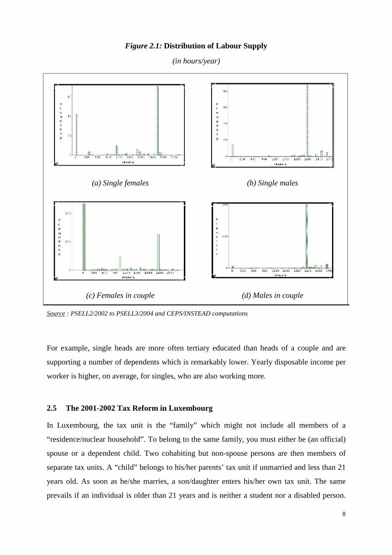
Figure 2.1 shows the labour supply under four nuclear household configurations: single

males, single females, males in couple and females in couple, whether dependents present in

the household or not. Clearly, little heterogeneity is observed for males where an

overwhelming majority is working exactly full-time (2080 hours/year12 in the present

framework). A few others mainly bunch around zero work effort for single males or more than

full-time for males in couple. This lack of heterogeneity on the male side is indeed

compromising the feasibility of a statistical estimation through the discrete choice modelling

under the latent class approach. We are then excluding single males from the present analysis

and assume a purely exogenous (hence “frozen”) labour supply for males in couple when

examining females in couple’s behaviour.

The two groups we are considering are composed of 162 “single” households headed by a

female (313 persons concerned) and 533 “couple” households (1,766 persons concerned)13 in

which both partners are selected workers. Table 2.2 gives some descriptive information about

the variables that will be used in the labour supply specifications for both single females and

females in couple. As expected, individual characteristics of heads of households often differ

when “singles” are compared to “couples”.

11 Given the rules for social assistance in Luxembourg, a decision taken by any member of a residence

household (for example, “not working”) can have an impact on the budget of other members of the household (for example, through minimum income scheme), which matters in the present analysis. Therefore, considering “nuclear” units as isolated each others would be unrealistic.

12 The full-time work is normalized to 2,080 hours per year (40 hours/week, 4.33 * 12 = 52 weeks/year). 13 The 695 selected persons marked as “workers” in our final sample represent 18% (weighted count) of the

population aged between 20 and 60 in the original PSELL3/2004 sample.

8

Figure 2.1: Distribution of Labour Supply

(in hours/year)

(a) Single females (b) Single males

(c) Females in couple (d) Males in couple

Source : PSELL2/2002 to PSELL3/2004 and CEPS/INSTEAD computations

For example, single heads are more often tertiary educated than heads of a couple and are

supporting a number of dependents which is remarkably lower. Yearly disposable income per

worker is higher, on average, for singles, who are also working more.

2.5 The 2001-2002 Tax Reform in Luxembourg

In Luxembourg, the tax unit is the “family” which might not include all members of a

“residence/nuclear household”. To belong to the same family, you must either be (an official)

spouse or a dependent child. Two cohabiting but non-spouse persons are then members of

separate tax units. A “child” belongs to his/her parents’ tax unit if unmarried and less than 21

years old. As soon as he/she marries, a son/daughter enters his/her own tax unit. The same

prevails if an individual is older than 21 years and is neither a student nor a disabled person.

9

Of course, the set of rules includes many other aspects, related to the questions of “earnings”

of dependent children, children living part-time only with their parents, status changing during

the civil year, spouses separating/being divorced, etc. These questions, although essential to

the system as a whole, are not discussed here.

Table 2.2: Descriptive Statistics of the Variables Relevant for the Labour Supply Specifications

Unweighted values (*)

Single females Females in couple

Variables Mean Standard deviation

Mean Standard deviation

Yearly disposable income (in EUR) 29,263 12,830 25,785 10,898

Yearly hours worked 1,319 896 900 915

Age 39.6 9.9 38.1 8.8

Education

Primary degree 28.4% 37.1%

High school degree 12.3% 11.8%

University degree 38.9% 33.9%

Higher Non-University degree 20.4% 17.1%

Children

Number of children 0.722 0.954 1.124 1.174

Number of children 0-5 0.167 0.435 0.396 0.679



Nationality

Luxembourgish 53.1% 43.7%

Portuguese 8.0% 23.1%

Other EU-15 31.5% 24.0%

Non-EU15 7.4% 9.2%

Number of observations 162 533

Source : EUROMOD input dataset (from PSELL2/2002 to PSELL3/2004) and CEPS/INSTEAD computations (through EUROMOD microsimulation for disposable income)

(*) The discrete choice modelling framework chosen in the present exploratory exercise does not take into account sample weighting. Therefore, all the results in the paper (including the present table) are shown unweighted.

10

The main outlines of the 2001-2002 reform in Luxembourg are described below:

- the first tax bracket is enlarged, which means that the minimum income before tax is

increased, from 6,693 EUR in 2000 up to 9,750 EUR in 2002;

- the number of tax brackets is reduced, from 18 down to 17 in 2002 and band widths are

made uniform to 1,650 EUR in 2002; and

- the maximum tax rate significantly decreases, from 46% to 38% in 2002.

The following methodological framework has been chosen for assessing the effects of such a

tax reform (see Liégeois et al., 2009).

We would like to strictly avoid changes not directly resulting from the tax reform or from a

modified labour supply. This is the reason why we choose to concentrate on a given year, as

far as the economy and the social field are concerned, with a simple treatment of the tax-

benefit environment. The year 2003 is chosen as a basis for analysis. In the benchmark, the

2003 tax system is designed conforming to the brief description earlier, which means in its

post-reform state. The alternative is then simply to set up (in 2003) the tax system as it was

before the 2001-2002 reform. On the benefit side, no change is to be mentioned between the

benchmark and the alternative. Altogether, these options raise the following question: What

would have happened for the population in 2003, had the 2000 tax system either been frozen

on the one side, or be replaced by the new 2003 tax system on the other side?

3. THEORETICAL AND EXMPIRICAL FRAMEWORKS FOR THE L ABOUR SUPPLY ANALYSIS

The model underlying the formation of labour supply is based on the neoclassical consumer

demand theory in which individuals make decisions about their hours worked (hence the time

devoted to leisure) and consumption by maximizing their utility subject to a specific budget

constraint and the total time endowment.

We describe the model (Section 3.1), specify its empirical implementation (Section 3.2) and

derive the likelihood function to be maximized (Section 3.3). Finally, the process is adjusted

in order to conform to economic rationality (Section 3.4).

11

3.1 Theoretical framework

The worker’s program can be written as:

Max

subject to

(1)

where:

U(.) : well-being index (utility function)

i : household’s index (i = 1, …, N)

: net disposable income of the household (= “consumption”, given our static

framework)

: labour supply by the head of household (either single female, or female in a

couple)

= total time endowment (T) – chosen level of leisure

: (a vector of) characteristics of the household

: non-labour income (all sources)

: all kinds of allowances (positive transfers)

: (all kinds of) taxes on labour income, non-labour income,

allowances

As explained earlier (cf. Section 1), we adopt the discrete choice approach regarding the

number of hours worked. These are to be chosen by the worker in finite set of distinct values.

Compared to the traditional (continuous) model, the main advantage of the discrete approach

is that a finite set of values only are to be computed for the well-being index and compared.

Then, an optimum is easily derived (see Figure 3.1). Moreover, the convexity of the budget

set and the piece-wise linearity of the budget line are not required. Finally, the coherency

conditions (monotonicity and quasi-concavity of the utility function) are not to be imposed a

12

priori but can be checked ex post14.

Figure 3.1: The Worker’s Program: Looking for an Optimum

(the indifference curves and the budget line are purely illustrative)

Remark : The well-being index U(.) including in the present analysis random

components (see infra), the “predicted” optimum for labour supply is indeed based on the combination (consumption, leisure) showing the highest probability (cf. Section 4.2).

3.2 Empirical Specification of the Utility Function

We assume a quadratic utility function (household’s index is omitted for simplicity):

(2)

where :

, , are coefficients

is denoting (indexing) the choice of labour supply : j = 1, … , J

h = h1, h2, … , hJ is the choice of labour supply, in a finite set of possibilities

14 For more details see MaCurdy et al. (1990) and Moffit (1990).

13

is a random disturbance (e.g. error made in evaluating alternative j) :

stands for “Type I extreme value distribution”, with cumulative density

.

The utility U(.) is classically assumed to be increasing with consumption y, and decreasing

with respect to hours worked h, even if those properties are not to be imposed a priori but can

be checked ex post. The total time endowment T is set to 4,000 hours per year.

Regarding the budget constraint in (1), the specification of the model allows for non-

convexities in the budget set and complex shapes for the budget line. These are unavoidable,

especially due to fixed costs and intricated rules for benefits and taxes: tax allowances

depending on whether the partner works or not, thresholds in social security premiums, etc.

Moreover, the budget constraint is to be evaluated for a finite set of hours-steps only (h1, h2,

… , hJ ).

The appropriate number of hours-steps is evaluated by looking at the mode value of the

histograms of hours worked for females (see Figures 2.1.a and 2.1.c). We consider three

choices for females: 0 (0 hour/year), 1040 (0+ up to 1500 hours/year), and 2080 (1500+

hours/year). The labour supply by males in a couple is exogenous and unchanged compared to

the level observed in the source data (cf. Section 2.3).

Furthermore, to account for preference variations across households, we need to specify the

nature of heterogeneity. For this, we assume that the preference parameters depend on the

person’s and household’s observed and unobserved characteristics. These characteristics are

likely to influence the preference for leisure. Hence the leisure coefficient is written as:

(3)

where the first part of the right member is relating to observed characteristics (in total there

are C = 4 different characteristics : age, education, nationality and the number of the children)

and the second part refers to unobserved (latent) characteristics15.

15 Heterogeneity is then enriching the well-being index and considering, beyond consumption and leisure as

such, several complementary individual and family dimensions, e.g., the number of children.

14

We follow Flood et al. (2004), which assumes that the unobserved heterogeneity capture the

effect of unobserved fixed costs of work as well as unobserved preferences for leisure. It is

worth mentioning that we do not have any explicit information on fixed costs in the data. This

is the reason why fixed costs variables are latent, unobserved variables in the model. They

comprise the costs of child care, commuting costs, etc. But they may also capture other

disincentives for paid work, such as search effort. It is indeed difficult to distinguish between

the various sources of fixed costs (van Soest et al. 2001) 16.

As unobserved heterogeneity (characteristics) θ is not observed, we specify a distribution for

it. We choose the latent class approach proposed by Heckman and Signer (1984)17 and assume

that there exists S different mass points for θ , each observed with probability sπ satisfying

Sss ..., 1, 10 =∀<=<= π and 11s

s =∑=

S

π . The major advantage of this approach is the

greater flexibility allowed in the labour supply modelling. The interpretation of this

unobserved heterogeneity parameter (mass points θ) is straightforward : the higher the value.

the stronger the preference for leisure.

3.3 Likelihood Function

Given the specification introduced in Section 3.2, it can be shown that for any household i and

given a mass point s (i = 1, …, N ; s = 1, …, S) :

(4)

where is the value of the utility function for household i, given his choice j for

labour supply.

16 Fixed cost was also included in the utility function with a dummy variable so that it captures the effect of the

cost only if the person is working. But the coefficient was not significant and didn’t improve the model with respect to likelihood ratio.

17 This approach has been applied in many other literatures, for example, in duration data (Ham and Lalonde, 1996), in count data (Deb and Trivedi, 1997) and in labour supply (Hoynes, 1996). Heckman and Singer (1984) also showed that estimation resulting from this approach might provide a good discrete approximation even if the underlying distribution is continuous.

15

It follows that the contribution of household i to the likelihood function is given by :

(5)

where is an indicator (1 or 0) that the state (labour supply) is the one observed for

the household under consideration.

Practically, the analytical expression for is derived from the (k = 1, …, J)

which in turn result from (2). For each hypothetical level of labour supply (h = h1, …, hJ), the

net income y in (2) is determined through EUROMOD microsimulation.

Finally, the likelihood function L can be written as:

(6)

Maximizing equation (6) yields estimates for the unknown coefficients of utility function

which, under general regularity assumptions, are consistent and asymptotically normal.

3.4 Adjusting the process to conform to economic rationality

Scientific literature often claims about discrete choice models that quasi-concavity of the

utility function is not obligatory, due to the fact that the utility is maximized over a finite set,

not requiring a tangency condition.

Nevertheless, the economic interpretation of the model is reasonably expecting a utility

function increasing with income18. This comes from the assumption that everyone prefers

consuming more, ceteris paribus, hence choosing a point on the frontier of the budget set. In

our results based on program (1)-(6), this condition is not fully satisfied. For example, around

17% of sample observations for females in couple do not satisfy the monotonicity condition.

Similar shortcoming is found in many other papers (see, for example, Lebeaga et al., 2008,

Van Soest and Das, 2001, and Vlasblom 1998).

16

To overcome this drawback, Van Soest and Das (2001) impose ad hoc parametric restrictions

a priori (hence reducing de facto the dimension of the parameter set), which are sufficient to

guarantee that marginal utility is positive ex post. Vlasblom (1998) avoids this by using a CES

utility function. However, those restrictions might sometimes appear to be unnecessarily too

severe. Alternatively, we complete the program (1)-(6) with necessary conditions (one per

household) imposing positive marginal utilities at optimum. We follow Islam and Liégeois

(2009) in which it has been shown that such a high-dimensional program can be equivalently

replaced by a one-dimensional one19. In the end, no observation shows negative marginal

utility at optimum.

4. STRUCTURAL ESTIMATES AND ANALYSIS OF THE LABO UR SUPPLY

We launch the analysis of the labour supply in Luxembourg regarding single females and

females in couple. The objective is to illustrate the link between individual characteristics or

wages and the choice of hours worked. We also examine how far the model properly fits

observed values for the labour supply in Luxembourg.

Structural estimates and the socio-economic properties of the well-being index are firstly

analyzed (Section 4.1). Then, predictions for the labour supply are formed from the model and

compared to the observed levels (Section 4.2). Finally, we examine the impact of an increase

in gross wages on labour supply and derive wage elasticities (Section 4.3).

4.1 Structural estimates and utility

We conduct similar analyses for single females and females in couple. The results are based

on equation (2) where the parameters are replaced by their estimated values shown in Tables

A1 and A2 in the Appendix.

It is well known that in a structural discrete choice specification, the estimated coefficients are

very difficult to interpret because they are not directly tied to the marginal effects of

characteristics on leisure and consumption. However, they give a hint about preferences.

Figure 4.1 represents the utility surface (a three-dimensional view from top) for a single

18 Taking first derivative of equation (2), marginal utility of income follows : )()(2 hTyU yhyyyy −++= βββ

17

Luxembourgish female aged 37 with one child and a higher non-university degree, an example

arbitrarily chosen in the sample. The computation is based on the estimated results20 presented

in Table A1. It can be seen that utility is increasing with income everywhere, which is

expected given the constraint imposed on the utility function (cf. Section 3.3). However, the

unconstrained marginal utility of leisure happens to be negative, especially for low income.

Figure 4.1: Utility Surfaces (Three-dimensional View from Top)

Single Luxembourgish female aged 37 with one young child and higher non-university degree

1000025000

4000055000

7000085000

0

10

20

30

40

50

60

70

14

00

16

00

18

00

20

00

22

00

24

00

26

00

28

00

30

00

32

00

34

00

36

00

38

00

40

00

Utility

Leisure (hours/year)

Income (EUR/year)

Source : EUROMOD input dataset (from PSELL2/2002 to PSELL3/2004) and CEPS/INSTEAD computations

(through EUROMOD microsimulation for disposable income)

Going further, it is very likely that females with young children have a stronger “preference”

for leisure. This is firstly illustrated through Figure 4.2, which represents indifference curves

for the same female as before. Solid lines refer to the “with one young child” case and dashed

lines refer to “no child”.

19 The likelihood function (6) is then maximized under a single constraint, and corresponding Kuhn-Tucker

conditions derived and solved.

20 We consider the expected value for unobserved characteristic θ .

18

Figure 4.2: Indifference Curves for a Female with a Young Child (Solid Lines) or Without a Child (dashed lines)

Single Luxembourgish female aged 37 with higher non-university degree

10

20

30

40

50

60

70

80

90

1,4 1,6 1,8 2 2,2 2,4 2,6 2,8 3 3,2 3,4 3,6 3,8 4

Dis

po

sab

le i

nc

om

e (

in t

ho

use

nd

EU

R/y

ea

r)

Leisure (in thousand hours / year) Source: EUROMOD input dataset (from PSELL2/2002 to PSELL3/2004) and CEPS/INSTEAD

computations (through EUROMOD microsimulation for disposable income)

Clearly, the marginal rate of substitution between leisure and income (slope of the

indifference curve) is higher for the mother, showing that a loss of leisure is to be

compensated by more additional consumption for the well-being keeping unchanged. For

lower income levels, the positive slopes of indifference curves result from utility decreasing

with leisure.

Complementarily, we can calculate the elasticity of substitution (linked to the curvature of the

indifference curve) for the same person at optimum when income is 62,114 EUR/year and

leisure is 1,920 hours/year (full-time worker). The elasticity of substitution is 0.77 for the

single female with one child and would be 0.71 without a child at the same point, which

shows up a higher “sensitivity” to relative changes in wages for the mother.

Aside from parenthood, other variables can play a role (see Tables A.1 and A.2). For example,

19

females with higher non-university degrees have significantly weaker preference for leisure,

compared to females with lower education and controlling for other characteristics. This result

is consistent whether they are single females or females in a couple.

Structural differences in labour supply behaviour may also depend on nationality. We find, for

example, that the non-EU15 single females have a stronger preference for leisure, compared to

Luxembourgish ones, contrarily to Portuguese and other EU-15s. Regarding couples again,

females show a preference for leisure depending negatively on their partner’s labour supply

and education when the partner has a university degree.

Hitherto, we have discussed how far females’ preferences are influenced by their observable

characteristics. But preferences may also vary with unobservable characteristics.

To evaluate such an impact, we have estimated the distribution of the unobservable

characteristics by latent class approach (cf. Section 3.2). Under such a framework, the model

appears to be well fitted21 with two types22 of unobserved heterogeneity (factors) determining

female’s preferences, each observed with an associated probabilityπ .

The results are presented in Tables A.1 and A.2. For example, for single females, the estimated

values 175.51 −=θ

and 065.02 =θ represent two types of unobservable factors with

corresponding estimated probabilities 41.01 =π and 59.02 =π . A possible interpretation is

that 59% of single females belong to a group showing a relatively stronger preference for

leisure (as 065.02 =θ > 175.51

−=θ ). Similarly, it appears that 20% of females in couple

have a stronger preference for work.

4.2 Prediction

The fit of the model can be judged according to its ability to properly predict the hours

worked.

We can, for example, compare the distribution of predicted hours given by the model to the

21 We compare the estimated results with and without unobserved characteristics for both single and females in

couple and find that preferences for leisure effectively depend on these unobserved factors.

22 S = 2, cf. Section 3.2. We have also tried to identify the model considering more than two types of unobserved factors, but the procedure could not converge. This is the limitation of latent class approach (there is a huge literature on this issue such as Hansen and Lofstrom 2001, Cameron and Heckman 2001, Stevens 1999, Ham and Lalonde 1996, Eberwein et al. 1997, Heckman and Singer 1984).

20

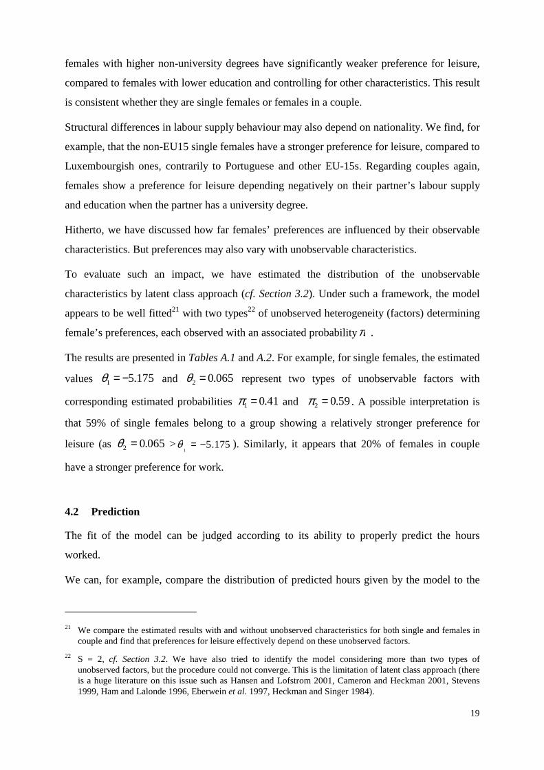
observed distribution23. Regarding the predicted outcome, the fitted probability values in

(4) are firstly computed using the parameter estimates in Tables A.1 and A.2 for single females

and females in couple respectively. Then, the labour supply prediction is here chosen based on

the highest probability. The distributions of observed hours worked, together with

distributions resulting from the prediction, are presented in Figures 4.3.

Figure 4.3: Observed and Predicted Labour Supply for Females in Luxembourg

Single female Female in couple

0

20

40

60

80

100

120

Not

working

Part

time

Full

time

No

. o

f I

nd

ifid

ua

ls

Observed

Predicted

0

50

100

150

200

250

300

350

Not

working

Part

time

Full

time

No

. o

f I

nd

ivid

ua

ls

Observed

Predicted

Source: EUROMOD input dataset (from PSELL2/2002 to PSELL3/2004) and CEPS/INSTEAD computations (through EUROMOD microsimulation for disposable income)

Notes: (a) Not working = 0 hour/year; Part-time = 0+ up to 1500 hours/year; Full-time = 1500+ hours/year.

(b) Labour supply decision of females in couple has been considered as a single decision, with partner’s earnings included in the female’s non-labour income.

The fit seems rather good, especially for single females, in the sense that predicted participation

rates and predicted average hours worked are very close to the corresponding observed values.

However, the model does not succeed in reproducing the distribution completely, especially for

females in couple. In particular, the model has a tendency to under-predict those cells with

small representations and over-predict others. This is a common difficulty with discrete choice

labour supply models (see, for details, Euwals and van Soest, 1999).

23 Of course, the observed distribution not only depends on the workers’ labour supply decisions, but also on the

demand of labour by firms : constraints or additional specificities on the demand side of the labour market, which are not taken into account here, do play a role as well.

21

4.3 Elasticity

As mentioned before, the estimated coefficients give very little information regarding the

effects of individual characteristics on preferences. An alternative to illustrate the results is to

compute the elasticity of labour supply with respect to the price of leisure, which is the wage

rate.

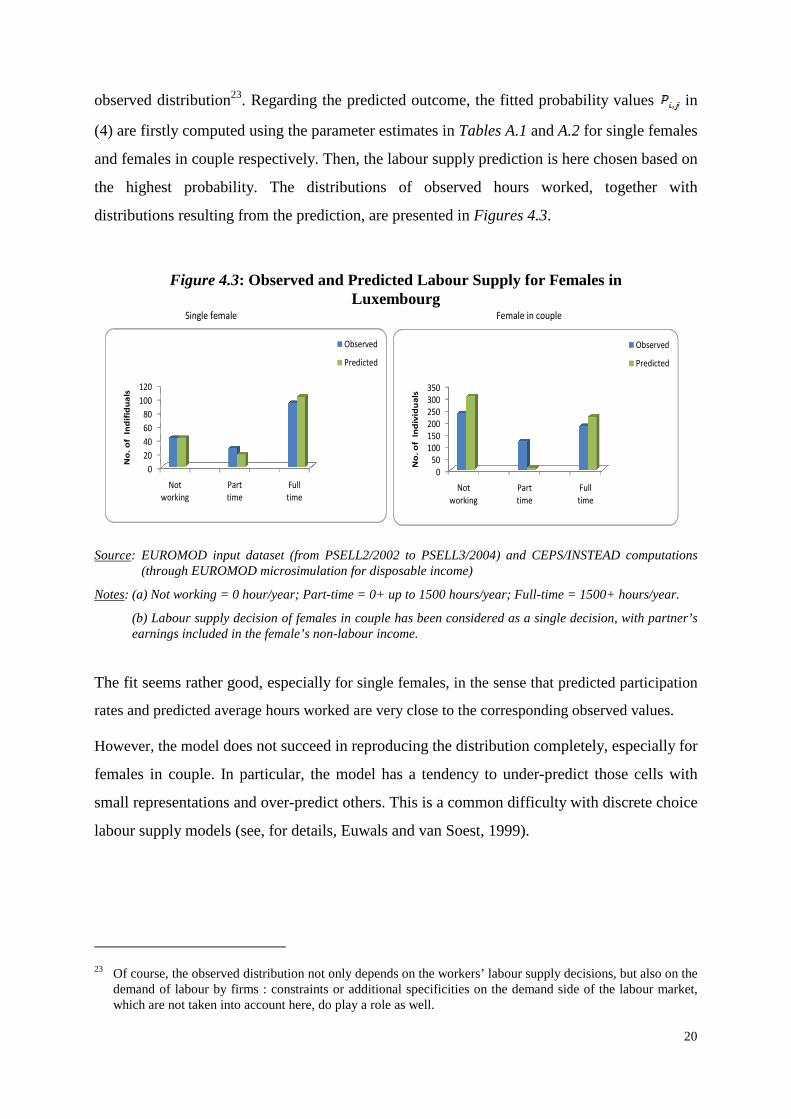
Table 4.1 summarizes the uncompensated wage elasticities of labour supply for single females

and females in couple and various quartile groups. The gross wage rate is increased by 10%

and the resulting disposable income of the households determined through EUROMOD

microsimulation24. Then, the “new” predicted labour supply is computed and compared to the

initial one (without the wage change) on an individual basis. Finally, elasticities are derived

from changes in the total labour supply by income group.

Table 4.1: The Wage Elasticity of Labour Supply, Overall and by Quartile of Income (Through a 10% wage increase)

Single females Females in Couple

Full sample 0.32 -0.28

1st quartile 1.25 -0.19

2nd quartile 0.57 -0.39

3rd quartile 0.14 -0.24

4th quartile 0.00 -0.26


Notes : a) The ranking on income is based on household total disposable income before the wage change (singles and couples separately);

b) Labour supply decision of females in couple has been considered as a single decision, with partner’s earnings included in the female’s non-labour income.

The results show that overall wage elasticities are rather small: a 10% wage increase raises

labour supply by about 3.2% (of hours worked) for single females and drops it by about 2.8%

for females in couple, on average.

Moreover, for single females only, a negative link between the wage elasticity and disposable

24 Of course, we consider here that no additional constraint happens due to the demand of labour by firms (see

previous footnote).

22

income is observed. But it must be remembered that if the relative gain in gross wage is 10%

for all here, the higher the quartile of income, the weaker the transposition in terms of net

disposable income, due to the progressivity of the tax system, ceteris paribus. Thus,

disparities in Table 4.1 result from both the socio-economic inter-quartile heterogeneity and

uneven transmission from gross to net along the income line.

The economic literature indeed confirms that the sign of the wage elasticity is ambiguous,

depending on the model specification and the data source (see, e.g., Kornstad and Thoresen,

2007). Moreover, a worker may have different wage elasticities, both in sign and magnitude,

depending on his position on the labour supply curve. The general picture in Table 4.1 is

therefore expected. This kind of diversified outcome is also visible in the next section, in

which tax reform induces changes in the labour supply that are not always qualitatively purely

in line with elasticities.

5. EFFECTS OF A TAX REFORM IN LUXEMBOURG

As an illustration, we analyze the effects of the significant 2001-2002 tax reform in

Luxembourg (cf. Section 2.5). The gain in income resulting from the reform is expected to

have a noticeable influence on the individual’s choice of hours worked.

The impact is firstly measured in terms of changes in the labour supply. Individual transitions

from one class of hours worked to another are examined and the overall impact is shown, by

quartile of disposable income and globally (Section 5.1). Then, the effects on disposable

income and well-being are presented, for the population as a whole and by quartile again.

Finally, the gain in disposable income is decomposed into behavioural effects (due to the

change in labour supply) and non-behavioural effect (due to the reform of the fiscal rules

alone) (Section 5.2).

5.1 Efficiency of the tax reform in terms of changes in the labour supply

At the individual level, the effects of the tax reform are summarized in a transition matrix

where rows i relate to the discrete distribution of hours worked with the reform and columns j

refer to what would be the discrete distribution of hours without the reform. Both distributions

are based on predicted values (cf. Section 4.2).

23

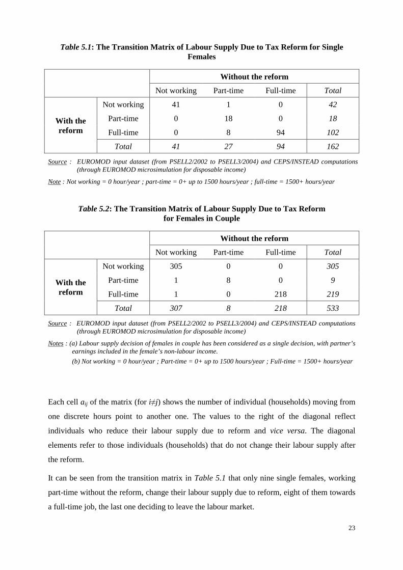
Table 5.1: The Transition Matrix of Labour Supply Due to Tax Reform for Single Females

Without the reform

Not working Part-time Full-time Total

With the reform

Not working 41 1 0 42

Part-time 0 18 0 18

Full-time 0 8 94 102

Total 41 27 94 162


Note : Not working = 0 hour/year ; part-time = 0+ up to 1500 hours/year ; full-time = 1500+ hours/year

Table 5.2: The Transition Matrix of Labour Supply Due to Tax Reform for Females in Couple

Without the reform

Not working Part-time Full-time Total

With the reform

Not working 305 0 0 305

Part-time 1 8 0 9

Full-time 1 0 218 219

Total 307 8 218 533


Notes : (a) Labour supply decision of females in couple has been considered as a single decision, with partner’s earnings included in the female’s non-labour income.

(b) Not working = 0 hour/year ; Part-time = 0+ up to 1500 hours/year ; Full-time = 1500+ hours/year

Each cell aij of the matrix (for i≠j) shows the number of individual (households) moving from

one discrete hours point to another one. The values to the right of the diagonal reflect

individuals who reduce their labour supply due to reform and vice versa. The diagonal

elements refer to those individuals (households) that do not change their labour supply after

the reform.

It can be seen from the transition matrix in Table 5.1 that only nine single females, working

part-time without the reform, change their labour supply due to reform, eight of them towards

a full-time job, the last one deciding to leave the labour market.

24

All other individuals remain on the diagonal, implying that the reform has limited impact on

the labour supply for single females25.

Regarding the females in couple, Table 5.2 shows that only two non-working females change

their position on the labour market. They join it, due to the reform.

The overall outcome for females in couple is clear: almost all of them stay on the diagonal of

the transition matrix, implying that the efficiency of the tax reform in terms of changes in the

labour supply is negligible.

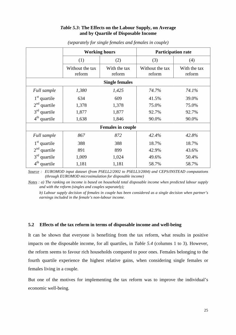
The results are confirmed at the macro level in Table 5.3 (Columns 1 and 2), with an increase

of the labour supply by 3.3% for single females, on average, and by 0.6% for females in

couple. Moreover, the participation rates are quasi-stable for both groups26 (Columns 3 and 4).

Nevertheless, in each reform, there are winners and losers. This is emphasized by the

distribution of the effects, which is not uniform over the quartiles of household disposable

income.

Table 5.3 shows that single females who belong to the second and third quartiles change

neither their labour supply nor their participation rate due to reform. By contrast, members of

the upper quartile increase their labour supply by 12.7% with the reform (despite a

participation rate to the labour market that remains unchanged), denoting a dominant price

effect for that class, whereas the poorest single females are deciding to work 3.9% less. For

females in couple, the reform leads to very little impact on the second and third quartiles

(+0.9% and +1.5% respectively).

25 This is qualitatively in line with results about the (low and positive) wage elasticity of labour supply (cf.

Section 4.3). Of course, the relation is weak given the complex nature of the tax reform, involving more than a simple homogenous increase in gross wages.

26 121 single females choose to work without the reform (out of 162 = 74.1%), while only 120 choose to work with the reform. For females in couple, there is a little increase from 226 to 228, out of 533.

25

Table 5.3: The Effects on the Labour Supply, on Average and by Quartile of Disposable Income

(separately for single females and females in couple)

Working hours Participation rate

(1) (2) (3) (4)

Without the tax reform

With the tax reform

Without the tax reform

With the tax reform

Single females

Full sample 1,380 1,425 74.7% 74.1%

1st quartile 634 609 41.5% 39.0%

2nd quartile 1,378 1,378 75.0% 75.0%

3rd quartile 1,877 1,877 92.7% 92.7%

4th quartile 1,638 1,846 90.0% 90.0%

Females in couple

Full sample 867 872 42.4% 42.8%

1st quartile 388 388 18.7% 18.7%

2nd quartile 891 899 42.9% 43.6%

3rd quartile 1,009 1,024 49.6% 50.4%

4th quartile 1,181 1,181 58.7% 58.7%


Notes : a) The ranking on income is based on household total disposable income when predicted labour supply and with the reform (singles and couples separately);

b) Labour supply decision of females in couple has been considered as a single decision when partner’s earnings included in the female’s non-labour income.

5.2 Effects of the tax reform in terms of disposable income and well-being

It can be shown that everyone is benefiting from the tax reform, what results in positive

impacts on the disposable income, for all quartiles, in Table 5.4 (columns 1 to 3). However,

the reform seems to favour rich households compared to poor ones. Females belonging to the

fourth quartile experience the highest relative gains, when considering single females or

females living in a couple.

But one of the motives for implementing the tax reform was to improve the individual’s

economic well-being.

26

Table 5.4: The Effects on the Household Disposable Income, on Average, by Quartile of Disposable Income and by Origin

(separately for single females and females in couple)

Disposable income

Equivalent variation

(EV, in EUR/year)

Decomposition (in % of gain of disposable income)

Without a tax reform

(in EUR/year)

With the tax

reform

(in EUR/year)

Gain due to

the reform (in %)

Behavioural effect (due

to labour supply)

Non-behavioural effect

(due to the reform of the fiscal rules)

(based on Predicted values, cf. Section 4.2) (Observed)

(1) (2)

(3) = (2) / (1) - 1 =

(5) + (6)

(4) (5) (6) (7)

Single females

Full sample 28,011 30,222 7.9% 1,326 3% 4.9% 5.0%

1st quartile 15,162 15,488 2.2% 393 -0.4% 2.5% 5.1%

2nd quartile 23,596 24,100 2.1% 504 0.0% 2.1% 2.6%

3rd quartile 30,793 32,656 6.1% 1,863 0.0% 6.1% 5.2%

4th quartile 42,746 48,951 14.5% 2,620 8.1% 6.5% 6.0%

Females in couple

Full sample 24,351 25,609 5.2% 1,222 0.2% 5.0% 5.1%

1st quartile 14,553 14,848 2.0% 295 0.0% 2.0% 2.8%

2nd quartile 19,978 20,623 3.2% 592 0.3% 3.0% 3.3%

3rd quartile 25,734 27,085 5.2% 1,258 0.4% 4.9% 5.2%

4th quartile 37,211 39,960 7.4% 2,749 0.0% 7.4% 6.9%


Notes : a) The ranking on income is based on household total disposable income when predicted labour supply and “with the reform” results (singles and couples separately);

b) Labour supply decision of females in couple has been considered as a single decision when partner’s earnings are included in the female’s non-labour income. The disposable income mentioned for the females in couple is half of the total household disposable income.

Clearly, we cannot measure the well-being (utility) through the disposable income (hence

consumption) only. The labour supply plays a role as well. It may be that a higher disposable

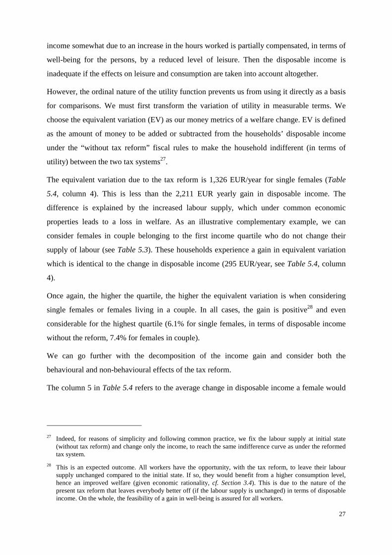
27

income somewhat due to an increase in the hours worked is partially compensated, in terms of

well-being for the persons, by a reduced level of leisure. Then the disposable income is

inadequate if the effects on leisure and consumption are taken into account altogether.

However, the ordinal nature of the utility function prevents us from using it directly as a basis

for comparisons. We must first transform the variation of utility in measurable terms. We

choose the equivalent variation (EV) as our money metrics of a welfare change. EV is defined

as the amount of money to be added or subtracted from the households’ disposable income

under the “without tax reform” fiscal rules to make the household indifferent (in terms of

utility) between the two tax systems27.

The equivalent variation due to the tax reform is 1,326 EUR/year for single females (Table

5.4, column 4). This is less than the 2,211 EUR yearly gain in disposable income. The

difference is explained by the increased labour supply, which under common economic

properties leads to a loss in welfare. As an illustrative complementary example, we can

consider females in couple belonging to the first income quartile who do not change their

supply of labour (see Table 5.3). These households experience a gain in equivalent variation

which is identical to the change in disposable income (295 EUR/year, see Table 5.4, column

4).

Once again, the higher the quartile, the higher the equivalent variation is when considering

single females or females living in a couple. In all cases, the gain is positive28 and even

considerable for the highest quartile (6.1% for single females, in terms of disposable income

without the reform, 7.4% for females in couple).

We can go further with the decomposition of the income gain and consider both the

behavioural and non-behavioural effects of the tax reform.

The column 5 in Table 5.4 refers to the average change in disposable income a female would

27 Indeed, for reasons of simplicity and following common practice, we fix the labour supply at initial state

(without tax reform) and change only the income, to reach the same indifference curve as under the reformed tax system.

28 This is an expected outcome. All workers have the opportunity, with the tax reform, to leave their labour supply unchanged compared to the initial state. If so, they would benefit from a higher consumption level, hence an improved welfare (given economic rationality, cf. Section 3.4). This is due to the nature of the present tax reform that leaves everybody better off (if the labour supply is unchanged) in terms of disposable income. On the whole, the feasibility of a gain in well-being is assured for all workers.

28

experience, with fiscal rules29 unchanged, hence due to the variation in her labour supply only

(columns 1 and 2, Table 5.3). This is the “pure” behavioural effect, which is nil, for example,

for single females belonging to the intermediate quartiles who do not adjust their labour

supply. However, the fiscal rules are reformed indeed, and a complementary non-behavioural

effect30 is generated (column 6 in Table 5.4).

Clearly, the behavioural effects appear to be negligible for most females, except for a single

female belonging to the upper quartile. For all others, the gain in disposable income largely

results from the change of the fiscal rules.

Most results in the Table 5.4 are derived from predicted values for the labour supply, for

comparability reasons. The last column only is based on “observed” levels for the labour

supply, directly copied from the input dataset. We can see from columns 7 and 6 that non-

behavioural effects computed from these alternative data31 are generally not too far, on

average, from outcome resulting from predicted values. Only the first quartile of single

females shows a clear divergence. This is an indication that we can be moderately confident in

the model, as far as such an analysis is concerned.

6. CONCLUSIONS

In this paper, we analyze the formation of labour supply decisions in Luxembourg.

We present a structural model in which the labour supply is treated as a discrete choice

problem and assume that these choices follow a simple conditional logit rule. The static

microsimulation model EUROMOD is used to evaluate consumption bundles corresponding

to different levels of hours worked (hence earnings). In addition, we allow for unobserved

individual-specific effects drawn from a discrete distribution. A coherency condition on the

marginal utility of consumption is imposed a priori, to allow for economic rationality, and is

taken into account during the estimation process. Under this framework, we analyze the

impact of an important tax reform that has been implemented in Luxembourg in 2001 and

29 Relating to the “with tax reform” case.

30 Fixing the labour supply at its “without tax reform” level.

31 Column 7 in Table 5.4 corresponds, for example, to the usual outcome of a EUROMOD microsimulation, in which the labour supply is constant and exogenous, directly and implicitly derived from input data, through the gross employment income variable.

29

2002.

Given the very limited heterogeneity of labour supply for males in the PSELL3/EU-SILC data,

we concentrate on females’ decisions only. Additionally, the nature of the model induces a

focus on residence households composed of one nuclear household only, either of single-type

or a couple.

Even if difficult to interpret, the estimated coefficients of the utility function show that the

marginal utility of leisure may be negative for lower disposable income households. We can

also observe, e.g., that females with young children have a stronger preference for leisure,

ceteris paribus. The same kind of preference prevails for about half of single females,

regarding their distribution of unobserved characteristics.

The fit of the model is rather good, especially for single females, in the sense that predicted

participation rates and predicted average hours worked are very close to the corresponding

observed values. However, the model does not succeed in reproducing the distribution

completely, especially for females in couple. In particular, there is a tendency to under-predict

those cells with small representations and over-predict others.

In terms of “reactivity”, the results show that overall wage elasticities are rather small: a 10%

wage increase raises labour supply by about 3.2% (of hours worked) for single females

(decreasing with the household disposable income quartile) and drops it by about 2.8% for

females in couple.

The 2001-2002 tax reform in Luxembourg, despite a significant change in the fiscal rules,

shows limited impact both in terms of transitions between one class of hours worked to

another and in terms of hours worked. Due to the reform, the labour supply increases by 3.3%

for single females, on average, and by 0.6% for females in couple. Nevertheless, the effects

may differ with income. For example, single females belonging to the upper quartile increase

their labour supply by 12.7% with the reform.

One of the motives for implementing the tax reform was to improve the individual’s economic

well-being and not the disposable income as such. It may be that a higher disposable income

due to an increase in the hours worked is partially compensated, in terms of well-being for the

person, by a reduced level of leisure. We compute the “equivalent variations” due to the

reform, a money metrics of the welfare change, and show, for example, that it is 1,326

30

EUR/year for single females. This is less than the 2,211 EUR yearly gains in disposable

income. The difference is explained by the observed increase in the labour supply.

Finally, we decompose the gain in disposable income into pure behavioural effect (due to

adjustments in labour supply only) and non-behavioural effect (labour supply unchanged). We

show that the former is negligible, compared to the latter, except for single females in the

upper income quartile.

More generally, the paper initiates an analysis of labour supply which is, as far as we know,

the first of its kind for Luxembourg. The message might be two-fold. First, the well-being

index obviously tells us more about actual welfare gains, which can differ a lot from changes

in the disposable income. Second, it appears that the behavioural component may be

negligible, but with noticeable exceptions like single females in the upper quartile (at least as

far as the 2001-2002 tax reform and our target population are concerned). This can be seen as

an encouragement to introduce such a component in static microsimulation models, as a

complementary module and certainly not as a unique and compulsory track.

Of course, we could go further and involve a larger sample of the resident population. We

could also test other policy reforms, but this is out of the scope of the present paper.

31

APPENDIX

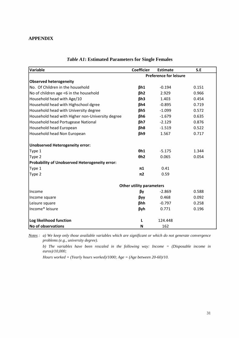
Table A1: Estimated Parameters for Single Females

Variable Coefficient Estimate S.E

Preference for leisure

Observed heterogeneity

No. Of Children in the household βh1 -0.194 0.151

No of children age <6 in the household βh2 2.929 0.966

Household head with Age/10 βh3 1.403 0.454

Household head with Highschool dgree βh4 -0.895 0.719

Household head with University degree βh5 -1.099 0.572

Household head with Higher non-University degree βh6 -1.679 0.635

Household head Portugease National βh7 -2.129 0.876

Household head European βh8 -1.519 0.522

Household head Non European βh9 1.567 0.717

Unobserved Heterogeneity error:

Type 1 θh1 -5.175 1.344

Type 2 θh2 0.065 0.054

Probability of Unobserved Heterogeneity error:

Type 1 π1 0.41

Type 2 π2 0.59

Other utility parameters

Income βy -2.869 0.588

Income square βyy 0.468 0.092

Leisure square βhh -0.797 0.258

Income* leisure βyh 0.771 0.196

Log likelihood function L 124.448

No of observations N 162

Notes : a) We keep only those available variables which are significant or which do not generate convergence problems (e.g., university degree).

b) The variables have been rescaled in the following way: Income = (Disposable income in euros)/10,000;

Hours worked = (Yearly hours worked)/1000; Age = (Age between 20-60)/10.

32

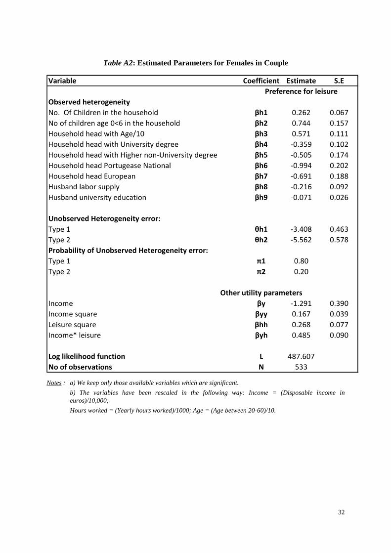
Table A2: Estimated Parameters for Females in Couple

Variable Coefficient Estimate S.E

Preference for leisure

Observed heterogeneity

No. Of Children in the household βh1 0.262 0.067

No of children age 0<6 in the household βh2 0.744 0.157

Household head with Age/10 βh3 0.571 0.111

Household head with University degree βh4 -0.359 0.102

Household head with Higher non-University degree βh5 -0.505 0.174

Household head Portugease National βh6 -0.994 0.202

Household head European βh7 -0.691 0.188

Husband labor supply βh8 -0.216 0.092

Husband university education βh9 -0.071 0.026

Unobserved Heterogeneity error:

Type 1 θh1 -3.408 0.463

Type 2 θh2 -5.562 0.578

Probability of Unobserved Heterogeneity error:

Type 1 π1 0.80

Type 2 π2 0.20

Other utility parameters

Income βy -1.291 0.390

Income square βyy 0.167 0.039

Leisure square βhh 0.268 0.077

Income* leisure βyh 0.485 0.090

Log likelihood function L 487.607

No of observations N 533

Notes : a) We keep only those available variables which are significant.

b) The variables have been rescaled in the following way: Income = (Disposable income in euros)/10,000;

Hours worked = (Yearly hours worked)/1000; Age = (Age between 20-60)/10.

33

BIBLIOGRAPHY

Bloemen, H.G., and A. Kapteyn. “The Estimation of Utility Consistent Labor Supply Models

by Means of Simulated Scores”. Journal of Applied Econometrics 23.4 (2008): 395-

422.

Blundell R., Duncan A., J. McCrae, and C. Meghir. “The Labour Market Impact of the

Working Families Tax Credit”. Fiscal Studies 21 (2000): 75-104.

Burtless G., and J. Hausman. “The Effect of Taxes on Labour Supply: Evaluating the Gray

Income Maintenance Experiment”. Journal of Political Economy 86.6 (1978): 1103-

30.

Cameron, S., and J.J. Heckman. “The Dynamics of Educational Attainment for Black,

Hispanic, and White Males”. Journal of Political Economy 109.3 (2001): 455-499.

Deb, P., and P. K. Trivedi., 1997. “Demand for Medical Care by the Elderly: A Finite Mixture

Approach”. Journal of Applied Econometrics 12 (1997): 313-336.

Eberwein, C., J. Ham, and R. Lalonde. “The Impact of Being Offered and Receiving

Classroom Training on the Employment Histories of Disadvantaged Females:

Evidence from Experimental Data”. Review of Economic Studies 64.4 (1997): 655-

682.

Euwals, R., and A. van Soest. “Desired and Actual Labor Supply of Unmarried Men and

Women in the Netherlands”. Labor Economics 6 (1999): 95-118.

Flood L.R., J. Hansen, and R. Wahlberg. “Household Labour Supply and Welfare

Participation in Sweden”. Journal of Human Resources 39.4 (2004): 1008-1032.

Ham, J., and R. Lalonde. “The Effect of Sample Selection and Initial Conditions in Duration

Models: Evidence from Experimental Data on Training”. Econometrica 64.1 (1996):

175-205.

Hansen, J., and M. Lofstrom. “The Dynamics of Immigrant Welfare and Labour Market

Behavior”. Discussion Paper no. 360 (2001), Institute for Study of Labour (IZA),

Bonn.

Heckman, J., and B. L. Singer. “A Method for Minimizing the Distributional Assumptions in

Econometric Models for Duration Data”. Econometrica 52 (1984): 271-320.

Hoynes, H.W. “Welfare Transfers in Two-Parent Families: Labour Supply and Welfare

Participation under AFDC-UP”. Econometrica 64 (1996): 295-332.

Islam, N., and Ph. Liégeois. “Dealing with Negative Marginal Utilities of Income in the

34

Discrete Choice Modeling of Labor Supply—A Technical Note”. Mimeo,

CEPS/INSTEAD (2009).

Keane, M., and R. Moffitt. “A Structural Model of Multiple Welfare Program Participation

and Labour Supply”. International Economic Review 39.3 (1998).

Kornstad, T., and T. O. Thoresen. “A Discrete Choice Model for Labor Supply and

Childcare”. Journal of Population Economics 20.4 (2007): 781-803.

Labeaga, M. José, X. Oliver, and A. Spadaro, “Discrete Choice Models of Labour Supply,

Behavioural Microsimulation and the Spanish Tax Reforms”. Journal of Economic

Inequality, Springer, vol. 6(3), pages 247-273, September (2008)

Liégeois, P., N. Islam, F. Berger, and R. Wagener. “Cross-validating Administrative and

Survey Datasets Through Microsimulation and the Assessment of a Tax Reform in

Luxembourg”. IRISS Working paper (2009): 2007-16.

Lucas, R. “Economic Policy Evaluation: A Critique”. Carnegie–Rochester Conference Series

on Public Policy 1 (1976): 19-46.

MaCurdy, T., D. Green, and H. Paarsch. “Assessing Empirical Approaches for Analyzing

Taxes and Labour Supply”. Journal of Human Resources 25 (1990): 1990.

Moffit, R. “ The Econometrics of Kinked Budget Constraints.” Journal of Economic

Perspectives 4:2 (Spring 1990).

Stevens, A. “Climbing Out of Poverty, Falling Back In”. Journal of Human Resources 34.3

(1999): 557-588.

Sutherland H., “EUROMOD: the tax-benefit microsimulation model for the European Union”

in Gupta A. and A. Harding (eds), Modelling Our Future: population ageing, health

and aged care. International Symposia in Economic Theory and Econometrics,

Vol 16, Elsevier (2007): 483-488.

Van Soest, A. “Structural Models of Family Labour Supply.” Journal of Human Resources 30

(1995): 63-28.

Van Soest, A., and M. Das. “Family Labour Supply and Proposed Tax Reform in the

Netherlands”. De Economist 149 (2001): 191-218.

Vlasblom, J.D. “Differences in Labour Supply and Income of Females in the Netherlands and

the Federal Republic of Germany”. Diss. University of Utrecht, 1998.

Discrete choice modelling of labour supply in Luxembourg through EUROMOD microsimulation

Documents