Estimation of consistent parameter sets for continuous-time nonlinear systems using occupation measures and LMI relaxations

Estimation of Consistent Parameter Sets for Continuous-time NonlinearSystems Using Occupation Measures and LMI Relaxations

Stefan Streif1, Philipp Rumschinski1, Didier Henrion2 and Rolf Findeisen1

Abstract— Obtaining initial conditions and parameterizationsleading to a model consistent with available measurementsor safety specifications is important for many applications.Examples include model (in-)validation, prediction, fault di-agnosis, and controller design. We present an approach todetermine inner- and outer-approximations of the set containingall consistent initial conditions/parameterizations for nonlinear(polynomial) continuous-time systems. These approximationsare found by occupation measures that encode the systemdynamics and measurements, and give rise to an infinite-dimensional linear program. We exploit the flexibility andlinearity of the decision problem to incorporate unknown-but-bounded and pointwise-in-time state and output constraints, afeature which was not addressed in previous works. The infinite-dimensional linear program is relaxed by a hierarchy of LMIproblems that provide certificates in case no consistent initialcondition/parameterization exists. Furthermore, the appliedLMI relaxation guarantees that the approximations converge(almost uniformly) to the true consistent set. We illustratethe approach with a biochemical reaction network involvingunknown initial conditions and parameters.

I. INTRODUCTION

The computation of guaranteed inner- and outer-approximations of consistent parameter sets of uncertain dy-namical systems is important for many applications includingmodel-based analysis and verification, system identification,model (in-)validation and controller design [1]–[4].

We consider the derivation of such approximations forpolynomial systems subject to unknown-but-bounded (orbounded-error) data. Different methods are available in liter-ature to address this problem. For discrete-time systems, forinstance interval analysis methods [5], or convex relaxation-based methods [6]–[9] can be employed. However, bothapproaches are not directly applicable to continuous-timesystems without additional assumptions. For instance in [10]it was assumed that the time-derivatives of the states areavailable as measurements, therefore, resulting in a steady-state problem similar to [11].

One possibility to address continuous-time systems withthe aforementioned methods is by discrete-time approxima-tions such as obtained by numerical integration schemes.However, due to the discretization error the consistent pa-rameter sets of continuous-time and discrete-time model donot necessarily overlap and, thus, wrong conclusions withrespect to model validity are possible [12].

1Laboratory for Systems Theory and Automatic Control, Institute for Au-tomation Engineering, Otto-von-Guericke-University Magdeburg, Germany.{stefan.streif,philipp.rumschinski,rolf.findeisen}@ovgu.de.

2LAAS-CNRS, Universite de Toulouse, France, and Faculty of Electri-cal Engineering, Czech Technical University in Prague, Czech [email protected]. This author acknowledges support by project 13-06894S of the Grant Agency of the Czech Republic.

Other estimation methods rely on numerical integrationand use higher-order Taylor approximations, resulting invalidated or verified integration methods [13]–[18], or dif-ferential inequalities (see [19] and references therein). Bydesign, these methods rely on numerical integrators.

There exist various methods using barrier certificates orsum-of-squares (SOS) polynomials [2]–[4], [20] which al-low the continuous-time dynamics to be considered directlywithout numerical integration. However, only few converseresults, i.e. existence of barrier certificates, are known andto the best of our knowledge no results with respect toapproximations of consistent parameter sets exist so far.

The main contribution of this work is the use of occupa-tion measures [21] to derive guaranteed polynomial inner-and outer-approximations of the consistent parameter setsfor continuous-time nonlinear (polynomial) systems basedon results presented in [22]–[24]. The reformulation interms of occupation measures leads to a linear but infinite-dimensional decision problem. However, its relaxation usingtruncated moment matrices and their dual SOS polynomi-als is a finite-dimensional convex problem. One particularfeature of the employed relaxation is the (almost uniform)asymptotic convergence of the approximations to the trueconsistent parameter set. Another advantage is that thecontinuous-time dynamics are completely encoded in thedecision problem and, thus, no numerical integration is nec-essary. Furthermore, we exploit the flexibility and linearityof the decision problem to incorporate unknown-but-boundedand pointwise-in-time state and output constraints, a featurewhich was not addressed in previous works.

This contribution is structured as follows. In Sec. II weformalize the problem setup, the considered system class, thedescription of the uncertain data and the desired propertiesof the approximations. To obtain constraints for a convexoptimization problem, we reformulate in Sec. III the poly-nomial continuous-time dynamics in terms of occupationmeasures. In Sec. IV, we adapt this approach to the con-sistent parameter estimation problem, which is reformulatedas an infinite-dimensional linear programming problem. Itssolution is approached numerically with a hierarchy of finite-dimensional semi-definite programs. We show how to deriveouter- and inner-approximations, as well as certificates ofinconsistency. The approach is demonstrated in Sec. V anddiscussed in Sec. VI.

II. PROBLEM FORMULATION

In this section we state the problem of set-based parameterestimation for continuous-time nonlinear systems of the

52nd IEEE Conference on Decision and ControlDecember 10-13, 2013. Florence, Italy

978-1-4673-5716-6/13/$31.00 ©2013 IEEE 6379

following form

x(t) = f(t, x(t)

), x(t0) = x0, (1a)

y(t) = h(t, x(t)

). (1b)

Here t ∈ [0, 1] is the time, the states are denoted by x ∈Rnx and the outputs by y ∈ Rny . Without loss of generalitythe terminal time is set to one by a suitable time-scaling ofthe dynamics. Initial conditions (at t = 0) are denoted byx0. We assume the vector field f : R × Rnx → Rnx andh : R × Rnx → Rny to be polynomial maps. To simplifynotation, we denote the state vector at time tk ∈ [0, 1] byxk = x(tk).

Note that time-invariant parameters p ∈ Rnp can beincluded in (1) by defining states with constant dynamics∀ i ∈ 1, . . . , np:

xi = fi(t, x(t)

)= 0, where pi := xi(0). (2)

That is, the state vector x contains nx − np true dynamicvariables and np constant parameters. The parameter valuesare then given by the initial conditions of the correspondingvariables xi. This formulation unifies the tasks of initialcondition and parameter estimation, and also simplifies thenotation and analysis (see next sections).

We assume that constraints on the states, output measure-ments and initial conditions (including the parameters) aregiven by polynomial inequalities g(·) ≥ 0. We rewrite theoutput constraints gy

(y(t)

)≥ 0 as state constraints using the

polynomial output map, i. e. gy(h(t, x)

)≥ 0.

Let mx time-independent constraints on the states be givenin the form x(t) ∈ X ,∀ t ∈ [0, 1] with

X :={x : gx,i

(x)≥ 0, ∀ i = 1, . . . ,mx

}⊂ Rnx . (3)

We additionally assume that we have a finite set of mt

distinct measurements at time points tk, k = 0, . . . ,mt − 1,such that: 0 = t0 < t1 < · · · < tmt−1 = 1. These timepoints include both the measurements of the output y(tk)and a priori information on the set of parameters and initialconditions. For each time point tk, let the constraints on thestates be given in the form xk ∈ Xk, k = 0, . . . ,mt−1 with

Xk :={x : gxk,i

(x)≥ 0, ∀ i = 1, . . . ,mxk

}⊆ X . (4)

Using this information, we want to estimate the consistentinitial conditions and parameters.

In the following, we denote the admissible state trajectory(an absolutely continuous function of time) of (1) starting atfixed x0 with x(t|x0), i. e.

x(t|x0) = x0 +

∫ t

0

f(τ, x(τ)

)dτ. (5)

Using (5), we define the set of consistent initial conditionsX ∗0 based on the set of consistent trajectories as follows:

X ∗0 :={x0 : ∃x(t|x0) s. t.

x(t|x0) ∈ X , ∀ t ∈ [0, T ] and (6)

x(tk|x0) ∈ Xk, ∀ k = 0, . . . ,mt − 1}.

With these notations, we can state the following problem:Problem 1 (Consistent parameter estimation). Find inner-

approximations I and outer-approximations O of consistentinitial conditions (parameters) such that I ⊆ X ∗0 ⊆ O.

For many applications such as model validation and faultdetection, it is sufficient to determine if the set X ∗0 is emptyor not, we therefore state the following related problem:Problem 2 (Certificate of inconsistency). If X ∗0 is empty,find a certificate of emptiness.

Consistency of a single initial condition x0 can easilybe checked numerically by solving equation (5). However,to determine the complete set X ∗0 is in general difficult,e. g. due to the involved nonlinearities and nonconvexities.We use occupation measures (see Sec. III) and convexrelaxations to derive the outer-approximation O based on[22]. The basic idea to find the inner-approximation I isto determine guaranteed enclosures of initial conditions thatviolate different constraints, cf. Sec. IV and [23]. Note thatthe inner-approximation I is given by the complement in Xof the union of these different enclosures.

In the next section, we describe how to deal with thecontinuous-time dynamics and state constraints using occu-pation measures. This enables us to derive convex optimiza-tion problems for the inner and outer-approximations.

III. OCCUPATION MEASURES ANDLIOUVILLE’S EQUATION

The crucial idea we employ in this work is to reformulatethe parameter estimation problem in terms of occupationmeasures. This has two main advantages. First, it allowsus to consider an entire distribution (or measure) of initialconditions and parameter values and not just single points.Second, linear relationships encoding the nonlinear dynamics(i.e. trajectories) of the system link these initial measureswith corresponding measures at the intermediate time-pointsfor which measurement data are available.

In [22] and the references therein, occupation measureswere used to estimate the region of attraction. Here wefirst review this approach, before we extend it for parameterestimation in Sec. IV. We show that unknown-but-boundedstate constraints at intermediate time points, not consideredin [22], can be handled easily. This is achieved by partition-ing the occupation measure w.r.t. a partitioning of the timeinterval, cf. Sec. IV. To determine the unknown occupationmeasures, a convex problem is derived. Albeit infinite-dimensional, the convex problem can be solved efficientlyby a hierarchy of finite-dimensional relaxations [22]–[24].

A. Occupation measures

Let M(A) denote the set of finite Borel measures sup-ported on the set A, which can be interpreted as elementsof the dual space C(A)′, i.e. as bounded linear functionalsacting on the set of continuous functions C(A). Let P (A)denote the set of probability measures on A, i.e. thosemeasures µ of M(A) which are nonnegative and normalizedto µ(A) = 1.

Now assume that the initial condition x0 is not preciselyknown, but that it can be interpreted as a random variable

6380

whose distribution is described by a probability measureµ0 ∈ P (X ). We define the occupation measure

µ(A× B) :=

∫T

∫XIA×B(t, x(t|x0))µ0(dx0) dt

for all subsets A × B in the Borel σ-algebra of subsets ofT × X , where T ⊂ R is a time interval and x(t|x0) is asin (5). Here, IA(x) is the indicator function of the set A,which is equal to one if x ∈ A, and zero otherwise.

Note that µ ∈ P (T × X ) is a probability measure, andthat the terminology occupation measure is motivated by theobservation that the value

∫T µ(dt,B) = µ(T × B) is equal

to the total time the trajectory spends in the set B ⊂ X . Inaddition, note that µ encodes the system trajectories, in thesense that if v ∈ C∞(T × X ;R) is a smooth test function,and if µ0 = δx0

is the Dirac measure at x0, integrationof v w.r.t. µ amounts to time integration along the systemtrajectory starting at x0:

〈v, µ〉 :=

∫T

∫Xv(t, x)µ(dt, dx) =

∫Tv(t, x(t|x0)

)dt.

The occupation measure µ can be disintegrated as µ(A×B) =

∫A µk(B|t) dt where conditional µk is a stochastic

kernel, in the sense that for every fixed t ∈ T , µk(dx|t) is aprobability measure on X describing the distribution of thestate x at time tk, and for every B ∈ X , t 7→ µk(B|t) is ameasurable function on T .

On the one hand, the introduced measures allow us toconsider the whole set of initial conditions (µ0). On theother hand, it allows a reformulation of the nonlinear dy-namics (1a) as a linear equation which only depends on theoccupation measures (µ, µtk ), as shown next.

B. Liouville’s equation

With these notations, for all sufficiently regular test func-tions v ∈ C1(T × X ;R) and T := [0, 1], it holds that∫

Xv(1, x)µ1(dx)−

∫Xv(0, x)µ0(dx) =∫

T

∫X

d

dtv(t, x(t|x0)

)µ0(dx0). (7)

The right-hand-side of the above equation can be rewritten∫T

∫X

( ∂∂tv(t, x(t|x0)

)+ grad v

(t, x(t|x0)

)·f(t, x(t|x0)

))µ0(dx0) dt

=

∫T

∫X

(∂

∂tv(t, x) + grad v(t, x) · f(t, x)

)µ(dt, dx).

To simplify notation, we introduce the Liouville operatorL : C1(T ×X )→ C(T ×X ) as Lv := ∂v

∂t +gradv ·f and itsadjoint L′ : C(T ×X )′ → C1(T ×X )′ such that 〈Lv, µ〉 =〈v,L′µ〉 for all v ∈ C1(T ×X ), i.e. L′µ := −∂µ∂t −div(µf).With these notations, (7) can be written concisely as

〈Lv, µ〉 = 〈v, δ1µ1〉 − 〈v, δ0µ0〉 (8)

for all v ∈ C1(T ×X ), where δ0 and δ1 refers to t = 0 andt = 1, respectively. Equivalently, in the sense of distributions,we can write

L′µ = δ1µ1 − δ0µ0. (9)

Equation (9) is Liouville’s equation and is also called thecontinuity equation in statistical physics or fluid mechanics.

Whereas the function x ∈ C(T ×X ) satisfies the nonlinearordinary differential equation (1a), the occupation measureµ ∈ P (T × X ) satisfies Liouville’s equation (9), which isa linear partial differential equation (PDE) in the space ofprobability measures.

Note that as the initial conditions are not known, themeasures are unknown as well. In the next sections we derivean optimization problem that allows us to determine theunknown measures.

C. Estimating the region of attraction

In [22] it was proved that the region of attraction X ∗0 ,defined as the set of initial conditions x0 consistent withthe dynamics (1a) and the constraints x(t) ∈ X , t ∈ Tand a constraint X1 at t = 1, is the support of the measureµ0 solving the infinite-dimensional linear programming (LP)problem

sup 〈1, µ0〉s.t. µ0 + µ0 = λ,

L′µ+ δ0µ0 − δ1µ1 = 0,

µ0 ≥ 0, µ0 ≥ 0, µ1 ≥ 0, µ ≥ 0,

(10)

where λ is the Lebesgue measure restricted to X , i.e. thestandard nx-dimensional volume. The supremum in (10) isw.r.t. measures µ0 ∈ P (X ), µ0 ∈ P (X ), µ1 ∈ P (X ) andµ ∈ P (T ×X ). Note that the slack measure µ0 results fromthe inequality µ0 ≤ λ as further explained in [22]. The aboveLP problem has a dual LP

inf 〈v0, λ〉s.t. v0(x) ≥ 0, ∀x ∈ X ,

v0(x) ≥ 1 + v(0, x), ∀x ∈ X ,v(1, x) ≥ 0, ∀x ∈ X1,

−Lv(t, x) ≥ 0, ∀ (t, x) ∈ T × X ,

(11)

where the infimum is w.r.t. continuous functions v0 ∈ C(X )and v ∈ C(T × X ).

The above LPs (10) and (11) are infinite-dimensional, be-cause the equations are required to hold for all test functionsv. One can solve these LPs by a converging hierarchy offinite-dimensional linear matrix inequality (LMI) problemsusing semidefinite programming. At a given relaxation orderd, the primal LMI is a moment relaxation of primal LP (10),whereas the dual LMI is a polynomial sum-of-squares (SOS)restriction of dual LP (11).

D. Sum-of-squares relaxation of the infinite dimensional LP

The dual LMI w.r.t. (11) is given byinf vc0

′l

s.t. −Lv(t, x) = p(t, x) + q0(t, x)t(1− t)+∑mxi=1 qi(t, x)gx,i(x),

v0(x) = v(0, x) + 1 + r0(x)

+∑mxi=1 r0,i(x)gx,i(x),

v0(x) = p0(x) +∑mxi=1 q0,i(x)gx,i(x),

v(1, x) = p1(x) +∑mxki=1 q1,i(x)gx1,i(x),

(12)

6381

where l is the vector of Lebesgue moments over X indexedin the same basis in which the polynomial v0(x) with coef-ficients vc0 is expressed. The minimum is over polynomialsv(t, x) and v0(x), and polynomial sum-of-squares p(t, x),q0(t, x), qi(t, x), p0(x), q0,i(x), p1(x), r0(x), r0,i(x),∀ i =1, . . . ,mx and q1,i(x),∀ i = 1, . . . ,mxk of appropriatedegrees. The constraints that polynomials are sum-of-squarescan be written explicitly as LMI constraints, and the objec-tive is linear in the coefficients of the polynomial v0(x).Therefore, problem (12) can be formulated as an SDP.

From the solution of the dual LMI of order d, we obtaina polynomial vd0(x) of given degree 2d which is such thatthe semialgebraic set Od := {x0 : vd0(x) ≥ 1} is a validouter-approximation of the region of attraction X ∗0 , i.e. X ∗0 ⊂Od. Moreover, the approximation converges in the Lebesguemeasure, or equivalently almost uniformly, in the sense thatlimd→∞ λ(Od) = λ(X ∗0 ), see [22] for details.

IV. CONSISTENT PARAMETER ESTIMATION

We use now the occupation measure approach to addressthe set-based parameter estimation Problems 1 and 2. Asshown next, this requires several extensions to be able toconsider the unknown-but-bounded state constraints at thedifferent measurement time-points tk.

First, we split the solution {x(t), t ∈ [0, 1]} of problem(1) into mt − 1 arcs {x(t), t ∈ Tk} with Tk := [tk, tk+1],k = 0, 1, . . . ,mt − 2. Now consider their respective occu-pation measures µk,k+1 ∈ M(Tk × X ), with intermediatemeasures µk ∈ P (Xk). Obviously

∑mt−2k=0 µk,k+1 = µ

and considering Liouville’s equation (9) on each arc of thetrajectory yields a system of linear PDEs

L′µk,k+1 = δtk+1µk+1 − δtkµk, k = 0, 1, . . . ,mt − 2.

A. Outer-approximation

An outer-approximation O ⊇ X ∗0 is given by the supportof the measure µ0 solving the LP

sup 〈1, µ0〉s.t. µ0 + µ0 = λ,

L′µk,k+1 = δtk+1µk+1 − δtkµk,

µ0 ≥ 0, µ0 ≥ 0,

µk+1 ≥ 0, µk,k+1 ≥ 0, k = 0, 1, . . . ,mt − 2,

(13)

where the supremum is w.r.t. measures µ0 ∈ P (X ), µ0 ∈P (X ), µk+1 ∈ P (Xk+1), µk,k+1 ∈ M([0, 1] × X ), k =0, 1, . . . ,mt − 2. The above LP problem has a dual LPinf 〈v0, λ〉s.t. v0(x) ≥ 0, ∀x ∈ X ,

v0(x) ≥ 1 + v0,1(0, x), ∀x ∈ X ,vk−1,k(tk, x) ≥ vk,k+1(tk, x), ∀x ∈ Xk,

k = 1, . . . ,mt−2,

vmt−2,mt−1(tmt−1, x) ≥ 0, ∀x ∈ Xmt−1,−Lvk,k+1(t, x) ≥ 0, ∀ (t, x) ∈ T × X ,

k = 0, 1, . . . ,mt−2,

(14)

where the infimum is w.r.t. continuous functions v0 ∈ C(X ),vk,k+1 ∈ C([0, 1],X ), k = 0, 1, . . . ,mt − 2.

As in Sec. III-C, the above infinite-dimensional LPs (13)and (14) are solved by a converging hierarchy of finite-dimensional LMI problems. From the solution of the dualLMI corresponding to (14) we obtain again a polynomialvd0(x) such that Od := {x0 : vd0 ≥ 1} ⊃ X ∗0 andlimd→∞ λ(X d0 ) = λ(X ∗0 ).

B. Inner-approximationFor the inner-approximation I ⊆ X ∗0 , we build on an

idea suggested in [23]. However, we have to take care ofthe different measurements at time-points tk, which requiresseveral extensions.

In the following, we consider the set of initial conditionsC∗0 for which there exists an admissible trajectory (5) thatviolates at least one of the constraints that define X and Xk.By continuity of solutions (the vector field f is polynomialand Lipschitz on the compact set X ), this set is equal to

C∗0 :=

x0 : ∃x(t|x0) s. t.

∃t ∈ [0, 1] and ∃ν s. t. gx,ν(x) < 0

or∃tκ and ∃η s. t. gxκ,η(x) < 0

, (15)

where ν = 1, . . . ,mx and η = 1, . . . ,mxk index the violatedconstraint, and κ = 0, . . . ,mt − 1 describes the time-points.Obviously X ∗0 := X \ C∗0 .

Note that depending on x(t|x0), there are different com-binations of constraints (gxκ,η and gx,ν) that can be violated.We directly deal with the different combinations and derivefor each one an outer-approximation of the set of initialconditions (and hence parameters) that lead to the violationof the constraint. As will be detailed in the sequel, theinner-approximation is then obtained from the union ofcomplements of these outer-approximations.

To simplify the presentation, we assume that the con-straints defining X are not violated, i.e. x(t|x0) ∈ X ,∀x0 ∈X0,∀ t ∈ T . This is a mild assumption, since the boundsX can often be derived from system insight (e.g. mass con-servation in chemical reaction networks), or can be chosensufficiently conservative. In any case, the constraints definingX can be treated similarly to Xk.

Note that the number of possible combinations, mc =2mtmxk − 1, can be very large. We can reduce the numberof combinations significantly due to the observation that ifone constraint at tκ is violated, then it does not matter if theconstraints for k > κ are satisfied or not and can thereforebe ignored. This can be formalized by:

Cκ,η :=

Xk = Xk, ∀ k < κ,

Xκ =

{x : gxκ,i(x) ≥ 0, ∀ i 6= η

gxκ,η(x) < 0

}, k = κ,

Xk = X , ∀ k > κ,

(16)

where i = 1, . . . ,mxk .Remark 1 (Strict and non-strict inequalities). In equa-tion (16), we consider strict inequalities. To account for strictinequalities small numbers (slack variables) are introducedwhen the LMIs are solved.

Then, once the mxkmt different outer-approximationsO(Cκ,η) have been determined, an inner-approximation is

6382

obtained by

I := X \⋃

κ=1,...,mt−1η=1,...,mxk

O(Cκ,η). (17)

C. Inconsistency certificate

Solving Problem 2, i.e. certifying emptiness of the setof consistent parameters X ∗0 , was not addressed in previ-ous work [22]. Mathematically, this amounts to certifyinginfeasibility of the infinite-dimensional LP

find µ0, µk, µmt−1, µk,k+1

s.t. µ0 + µ0 = λ,

L′µk,k+1 = δtk+1µk+1 − δtkµk, (18)

µ0 ≥ 0, µ0 ≥ 0,

µk+1 ≥ 0, µk,k+1 ≥ 0, k = 0, 1, . . . ,mt − 2,

which corresponds to (13) without a cost function. Wecan check that we meet all the assumptions to apply thegeneralized Farkas’ theorem of [25, Theorem 2] and thatnon-existence of measures µ0, µk, µmt−1, µk,k+1 solving LPproblem (18) is equivalent to the existence of continuousfunctions v0, v solving the dual LPfind µ0, µk, µmt−1, µk,k+1, k = 1, . . . ,mt − 2,

s.t. 〈v0, λ〉 = −1,

v0(x) ≥ 0, ∀x ∈ X ,v0(x) ≥ 1 + v0,1(0, x), ∀x ∈ X ,vk−1,k(tk, x) ≥ vk,k+1(tk, x), ∀x ∈ Xk,

k = 1, . . . ,mt − 2,

vmt−2,mt−1(tmt−1, x) ≥ 0, ∀x ∈ Xmt−1,−Lvk,k+1(t, x) ≥ 0, ∀ (t, x) ∈ T × X ,

k = 0, 1, . . . ,mt − 2,

(19)

If X ∗0 is empty, then LP problem (13) is infeasible. If anLMI relaxation of problem (13) is infeasible at some orderd, which can be certified by a normalized Farkas’ vector asa result of the dual LMI relaxation of (19) (cf. Sec. III-D),then LP (13) is also infeasible. Thus, finding a normalizedFarkas’ vector gives a sufficient condition that can be usedto provide a certificate of inconsistency.

V. EXAMPLE

We consider a biochemical reaction network in which thesubstrate x1 is enzymatically converted into a product via in-termediary complex x2 [26]. The continuous-time dynamicsis given by:

x1(t) = −p1 x1(t)(1− x2(t)

)+ p2 x2(t),

x2(t) = p1 x1(t)(1− x2(t)

)−(p2 + p3

)x2(t).

(20)

The following constraints on the parameters and stateswere used:

X :

{(pi − 0.1)(10− pi) ≥ 0, i = 1, 2, 3,

xi(1− xi) ≥ 0, i = 1, 2.

Measurement constraints Xk were generated from a simu-lated nominal trajectory with p1 = p2 = p3 = 5.05, x1(0) =0.9 and x2(0) = 0.05. An absolute uncertainty of ±0.025was added to the nominal values at the measurement time

points t0 = 0, t1 = 0.3, t2 = 1 to obtain X0, X1, X2. Thus,at each time-point four constraints were used, which resultsin mc = 4 · 3. To avoid numerical troubles, note that thedynamics (20) and X were scaled such that the values ofthe parameters range from 0 to 1.

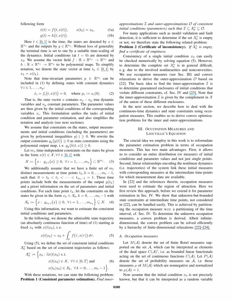
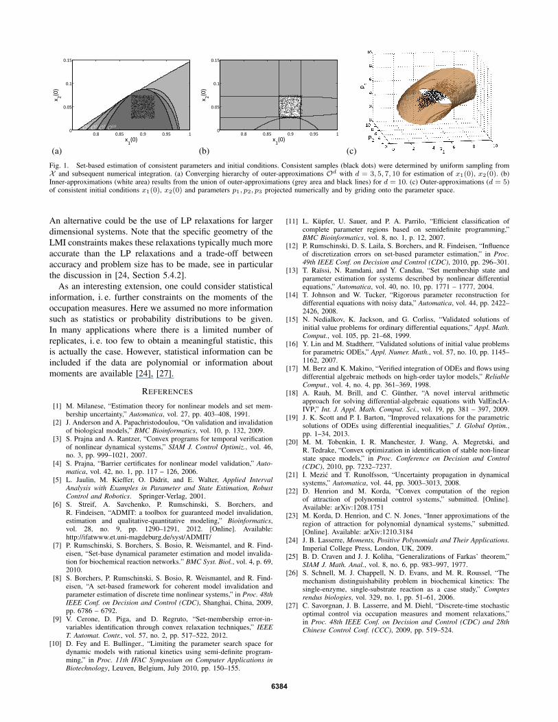
As can be seen in Fig. 1, the sequence of outer-approximations Od converges to the consistent parameter setfor increasing d. Using YALMIP and MOSEK7 on a standarddesktop PC, the solving time was about 7 sec for d = 3, and13 min for d = 10.

The inner-approximation in Fig. 1(b) correspondsto the complement (in X ) of the union of twelveouter-approximations O(Ci). However, only five outer-approximations are shown since the other four were empty.Solving time was on average 4.5 min per problem.

In addition we determined the outer-approximation ofconsistent initial conditions x1(0), x2(0) and parametersp1, p2, p3, see Fig. 1(c). Solving time was about 4.5 hrs ford = 3 and 7.5 hrs for d = 5.

Note that the inconsistency certificates derived in Sec-tion IV-C could also be used to invalidate entire regions inthe space of the parameters and initial conditions.

VI. DISCUSSION AND CONCLUSIONS

Occupation measures are a classical tool in kinetic theory,statistical physics, optimal transport, Markov decision pro-cesses, amongst others. In a broad perspective, the potentialof occupation measures and subsequent convex relaxationsare not often used in systems control. We used occu-pation measures to approximate consistent parameter setsfor continuous-time nonlinear systems without the need ofnumerical integration. A particular feature of the derived ap-proximations is the (almost uniform) convergence to the true(possibly nonconvex) consistent parameter set. As demon-strated at the example, outer- and inner-approximationscan be obtained even though only few measurements withrelatively large error are used. Tighter approximations areexpected if more measurements are used, or if e. g. outer-approximations are iteratively used to refine the results as itproved useful for linear relaxations [6]–[8].

While inconsistency certificates can be used to proveinconsistency of entire models or parameter regions, theouter- and inner-approximations can be used to get the shapeof the consistent parameter set. Such a description of theouter-approximation by a single polynomial can be veryuseful in some applications. In other cases different typesof representations like a collection of half-spaces might bemore beneficial. The inconsistency certificates could also beused to derive in an iterative and recursive manner eitherouter bounding boxes or a description of the consistent setusing a bisection algorithms (cf. [6]).

A drawback of the presented approach is the computa-tional workload resulting from the LMI constraints. Theo-retically, the resulting problems can be solved in polyno-mial time w.r.t. the input size. However, due to the sizelimitations of state-of-the-art SDP solvers, this approach isat the moment restricted to problems of small dimensions.

6383

(a)x1(0)

x 2(0)

0.8 0.85 0.9 0.95 10

0.05

0.1

0.15

O10O7O5O3

(b)x1(0)

x 2(0)

0.8 0.85 0.9 0.95 10

0.05

0.1

0.15

(c)

Fig. 1. Set-based estimation of consistent parameters and initial conditions. Consistent samples (black dots) were determined by uniform sampling fromX and subsequent numerical integration. (a) Converging hierarchy of outer-approximations Od with d = 3, 5, 7, 10 for estimation of x1(0), x2(0). (b)Inner-approximations (white area) results from the union of outer-approximations (grey area and black lines) for d = 10. (c) Outer-approximations (d = 5)of consistent initial conditions x1(0), x2(0) and parameters p1, p2, p3 projected numerically and by griding onto the parameter space.

An alternative could be the use of LP relaxations for largerdimensional systems. Note that the specific geometry of theLMI constraints makes these relaxations typically much moreaccurate than the LP relaxations and a trade-off betweenaccuracy and problem size has to be made, see in particularthe discussion in [24, Section 5.4.2].

As an interesting extension, one could consider statisticalinformation, i. e. further constraints on the moments of theoccupation measures. Here we assumed no more informationsuch as statistics or probability distributions to be given.In many applications where there is a limited number ofreplicates, i. e. too few to obtain a meaningful statistic, thisis actually the case. However, statistical information can beincluded if the data are polynomial or information aboutmoments are available [24], [27].

REFERENCES

[1] M. Milanese, “Estimation theory for nonlinear models and set mem-bership uncertainty,” Automatica, vol. 27, pp. 403–408, 1991.

[2] J. Anderson and A. Papachristodoulou, “On validation and invalidationof biological models,” BMC Bioinformatics, vol. 10, p. 132, 2009.

[3] S. Prajna and A. Rantzer, “Convex programs for temporal verificationof nonlinear dynamical systems,” SIAM J. Control Optimiz., vol. 46,no. 3, pp. 999–1021, 2007.

[4] S. Prajna, “Barrier certificates for nonlinear model validation,” Auto-matica, vol. 42, no. 1, pp. 117 – 126, 2006.

[5] L. Jaulin, M. Kieffer, O. Didrit, and E. Walter, Applied IntervalAnalysis with Examples in Parameter and State Estimation, RobustControl and Robotics. Springer-Verlag, 2001.

[6] S. Streif, A. Savchenko, P. Rumschinski, S. Borchers, andR. Findeisen, “ADMIT: a toolbox for guaranteed model invalidation,estimation and qualitative-quantitative modeling,” Bioinformatics,vol. 28, no. 9, pp. 1290–1291, 2012. [Online]. Available:http://ifatwww.et.uni-magdeburg.de/syst/ADMIT/

[7] P. Rumschinski, S. Borchers, S. Bosio, R. Weismantel, and R. Find-eisen, “Set-base dynamical parameter estimation and model invalida-tion for biochemical reaction networks.” BMC Syst. Biol., vol. 4, p. 69,2010.

[8] S. Borchers, P. Rumschinski, S. Bosio, R. Weismantel, and R. Find-eisen, “A set-based framework for coherent model invalidation andparameter estimation of discrete time nonlinear systems,” in Proc. 48thIEEE Conf. on Decision and Control (CDC), Shanghai, China, 2009,pp. 6786 – 6792.

[9] V. Cerone, D. Piga, and D. Regruto, “Set-membership error-in-variables identification through convex relaxation techniques,” IEEET. Automat. Contr., vol. 57, no. 2, pp. 517–522, 2012.

[10] D. Fey and E. Bullinger., “Limiting the parameter search space fordynamic models with rational kinetics using semi-definite program-ming,” in Proc. 11th IFAC Symposium on Computer Applications inBiotechnology, Leuven, Belgium, July 2010, pp. 150–155.

[11] L. Kupfer, U. Sauer, and P. A. Parrilo, “Efficient classification ofcomplete parameter regions based on semidefinite programming,”BMC Bioinformatics, vol. 8, no. 1, p. 12, 2007.

[12] P. Rumschinski, D. S. Laila, S. Borchers, and R. Findeisen, “Influenceof discretization errors on set-based parameter estimation,” in Proc.49th IEEE Conf. on Decision and Control (CDC), 2010, pp. 296–301.

[13] T. Raıssi, N. Ramdani, and Y. Candau, “Set membership state andparameter estimation for systems described by nonlinear differentialequations,” Automatica, vol. 40, no. 10, pp. 1771 – 1777, 2004.

[14] T. Johnson and W. Tucker, “Rigorous parameter reconstruction fordifferential equations with noisy data,” Automatica, vol. 44, pp. 2422–2426, 2008.

[15] N. Nedialkov, K. Jackson, and G. Corliss, “Validated solutions ofinitial value problems for ordinary differential equations,” Appl. Math.Comput., vol. 105, pp. 21–68, 1999.

[16] Y. Lin and M. Stadtherr, “Validated solutions of initial value problemsfor parametric ODEs,” Appl. Numer. Math., vol. 57, no. 10, pp. 1145–1162, 2007.

[17] M. Berz and K. Makino, “Verified integration of ODEs and flows usingdifferential algebraic methods on high-order taylor models,” ReliableComput., vol. 4, no. 4, pp. 361–369, 1998.

[18] A. Rauh, M. Brill, and C. Gunther, “A novel interval arithmeticapproach for solving differential-algebraic equations with ValEncIA-IVP,” Int. J. Appl. Math. Comput. Sci., vol. 19, pp. 381 – 397, 2009.

[19] J. K. Scott and P. I. Barton, “Improved relaxations for the parametricsolutions of ODEs using differential inequalities,” J. Global Optim.,pp. 1–34, 2013.

[20] M. M. Tobenkin, I. R. Manchester, J. Wang, A. Megretski, andR. Tedrake, “Convex optimization in identification of stable non-linearstate space models,” in Proc. Conference on Decision and Control(CDC), 2010, pp. 7232–7237.

[21] I. Mezic and T. Runolfsson, “Uncertainty propagation in dynamicalsystems,” Automatica, vol. 44, pp. 3003–3013, 2008.

[22] D. Henrion and M. Korda, “Convex computation of the regionof attraction of polynomial control systems,” submitted. [Online].Available: arXiv:1208.1751

[23] M. Korda, D. Henrion, and C. N. Jones, “Inner approximations of theregion of attraction for polynomial dynamical systems,” submitted.[Online]. Available: arXiv:1210.3184

[24] J. B. Lasserre, Moments, Positive Polynomials and Their Applications.Imperial College Press, London, UK, 2009.

[25] B. D. Craven and J. J. Koliha, “Generalizations of Farkas’ theorem,”SIAM J. Math. Anal., vol. 8, no. 6, pp. 983–997, 1977.

[26] S. Schnell, M. J. Chappell, N. D. Evans, and M. R. Roussel, “Themechanism distinguishability problem in biochemical kinetics: Thesingle-enzyme, single-substrate reaction as a case study,” Comptesrendus biologies, vol. 329, no. 1, pp. 51–61, 2006.

[27] C. Savorgnan, J. B. Lasserre, and M. Diehl, “Discrete-time stochasticoptimal control via occupation measures and moment relaxations,”in Proc. 48th IEEE Conf. on Decision and Control (CDC) and 28thChinese Control Conf. (CCC), 2009, pp. 519–524.

6384