Eleftherios Mylonas , Nikolaos Tzanis , Michael Birbas ...

electronics

Article

An Automatic Design Framework for Real-TimePower System Simulators Supporting SmartGrid Applications

Eleftherios Mylonas , Nikolaos Tzanis , Michael Birbas * and Alexios Birbas

Electrical and Computer Engineering Department, University of Patras, 26504 Patras, Greece;[email protected] (E.M.); [email protected] (N.T.); [email protected] (A.B.)* Correspondence: [email protected]

Received: 10 December 2019; Accepted: 24 January 2020; Published: 9 February 2020

Abstract: Smart grid technology is the next step to the evolution of classical power grids, providingrobustness, reliability, and security throughout the network, enabling real-time management andcontrol. To achieve these goals, distributed computing (microgrid concept) and intelligent controlalgorithms, tailored to the nature and needs of the network under study, are necessary. To dealwith the vast diversity of power grids, being able to capture the dynamics of any given network,and create tools for network analysis, apparatus testing, and power grid management, an automaticdesign framework for real-time power system simulators is needed. In this article, a prototype ofthis approach is presented, employing Field Programmable Gate Array (FPGA) platforms dueto their reconfigurability that enables low-power, low-latency, and high-performance designs,as a first attempt towards an open source platform, compatible with the majority of hardwaredesign suites. It comprises two major parts: (i) a user-oriented section, built in Matlab/Simulink;and (ii) a hardware-oriented section, written in Matlab and Very High Speed Integrated Circuit(VHSIC)-Hardware Description Language (VHDL) code. To verify its functionality, two test powernetworks were given in a schematic format, analyzed through Matlab code and turned into dedicatedhardware simulators with the aid of the VHDL template. Then, simulation results from Simulinkand the prototype were compared for error estimation. The results show the prototype’s successfulimplementation with minimal resources utilization, high performance and low latency in the order ofnanoseconds in Xilinx 6- and 7-series FPGAs, therefore proving its modularity and efficient use inmany different scenarios, meeting low-latency/real-time requirements while enabling further smartgrid research.

Keywords: smart grids; power system simulation; real-time simulation; design automation;computing systems; embedded systems; software/hardware design; FPGAs

1. Introduction

Smart grid is a term used to describe the classical power grid enhanced with “intelligence” [1],in the sense that a logical layer (intelligence) is placed on top of the physical system, controlling itsoperation in real-time. This (logical) layer is composed of many different functional units, such asdigital platforms, dedicated software and hardware accelerators which host the system’s logic, as wellas from a trusted communication layer. Utilizing these resources, the smart grid integrates advancedcomputing and communication technologies in order to provide “smart” services to energy producersand consumers, while increasing the system’s reliability, security, efficiency, and resilience. In a smart gridframework (Figure 1) [2], the increasing energy demands of society, the problems and the constraints ofthe current power network infrastructure, the inclusion of numerous Renewable Energy Sources (RESs),the management of Distributed Energy Resources (DERs), and the control of a strongly heterogeneous

Electronics 2020, 9, 299; doi:10.3390/electronics9020299 www.mdpi.com/journal/electronics

Electronics 2020, 9, 299 2 of 24

system are crucial parameters that should be taken into account. Therefore, intelligence at the energygrid is of paramount importance for creating a modern, dynamic, and robust power system.

Figure 1. Smart grid concept.

The ongoing research regarding smart grid technology faces many challenges of different difficultylevels and nature. This is due to the multidimensionality of the smart grid problem, which requires thecombination of knowledge from different fields, e.g., power systems, communications, informationtechnology, cyber-physical systems, Artificial Intelligence (AI), control theory, and economics. Mostsmart grid problems, e.g., optimal energy distribution, load balancing, load forecasting, transactiveenergy market, etc., require real-time monitoring and computing capabilities over the power grid sothat system operators, utility companies, as well as consumers can monitor, process, and act uponimportant system data on-the-fly. For example, regarding the demand response management problem,especially when dealing with deregulated market models, the utility companies and the consumersneed to solve game-like optimization problems to achieve balance between pricing and energy demand,while minimizing their respected costs [3,4]. The accurate real-time monitoring/prediction of theconsumers’ energy demand eliminates this problem, by performing real-time simulation, possiblyaided by conducting computations at the edge of the network. It can be easily inferred that smart gridproblems require real-time simulation/monitoring, which facilitates the potential forthcoming needsof such dynamic environments.

Many state-of-the-art technologies have been considered to support the smart grid framework [5].5G technology has been proposed to meet the smart grid’s strict time requirements across its boundaries,to achieve real-time monitoring and control. Furthermore, Internet of Things (IoT) platforms are used inthe smart grid context to define rules for communication, sharing and processing of data among sensors,smart meters, controllers and data centers; ease service applications’ design; and provide energy clientswith ubiquitous access to smart services. For the “intelligent” part, many Machine Learning (ML) anddeep learning techniques are available for high precision data analysis, while acceleration of suchtasks to achieve real-time execution is possible thanks to the broad use of Field Programmable GateArray (FPGA) platforms, which utilize special integrated circuits capable of addressing various, hardcomputing tasks due to their internal design, enabling them to be reconfigurable and to their inherentcapability for even massive parallelism. However, there are still several issues to be addressed [6].Some of the most critical are the grid’s complexity and size, and its security and dynamic management.To alleviate these problems, the microgrid concept is adopted. Microgrids—small-scale smart gridsoperating in a semi-autonomous manner—help to share/distribute the heavy network managementworkload to many small, easily managed and more secure networks, thus reducing the time forapplying control actions and strengthening the overall system against cyber attacks.

Electronics 2020, 9, 299 3 of 24

Although microgrids are able to respond quickly to transient phenomena, the microgrid controllogic should be customized to the underlying network to achieve best results. However, this isnot a simple task as microgrids are expected to be highly diverse, therefore demanding a solutionthat provides flexibility. In that respect, we propose an automatic design framework for real-timepower system simulators in the context of microgrid analysis, targeting FPGA platforms for theirinherent parallelism, needed for achieving high performance and latency in the order of tenths ofnanoseconds, and reconfigurability, which provides increased flexibility compared to other alternatives,e.g., General-Purpose Graphics Processing Units (GPGPUs). This concept of creating fully automatedsoftware platforms for providing simplicity and reducing production costs is not quite new. In powergrid applications, software suites such as Matlab/Simulink, EMTDC/PSCAD [7], and EMTP [8,9]support this idea. In the context of real-time power system simulation, OPAL-RT [10] and TyphoonHIL [11] are two representative examples showcasing the increasing need for FPGA-based simulationplatforms from the industry, which are, however, usually characterized of high cost. Additionally,in the last few years, researchers around the world have been trying to address this matter, creatinga basis literature around this topic [12,13]. In that regard, our work is a first attempt to create a low-cost,full-solution platform targeting microgrids that provides the necessary tools, and enables the user todesign custom power system hardware (through such a simulator) with much less effort. Moreover,this framework is the first step towards our vision of the design of a fully open source platform, whichwill contribute in the research towards power electronics, power grid design, and smart grid relatedtopics, such as the enabling of intelligent, low latency microgrid control algorithms.

In this article, our automatic design framework for real-time power system simulators is proposedand a prototype implementation is provided. The logic diagram of the framework is presentedin Figure 2. According to this, the power system simulator design is divided into two sections:the user-oriented and the hardware-oriented ones. In the user-oriented section, a General UserInterface (GUI) is provided, where the schematic of any system under study can be created. In addition,a software library comprising component models and a network analysis algorithm are utilizedin order to extract the system information in a compatible format for hardware implementation.Our network analysis algorithm simplifies the complexity of the simulation by applying graphoptimizations where possible. Moreover, to further expand the library of compatible componentstowards creating a complete software toolkit, a library of complex component models and errorestimation support are included. In the hardware-oriented section, a special module helps the userspecify the fixed-point data representation for the simulation of the given network according toapplication-specific criteria, which usually are sufficient precision and low memory footprint. Lastly,a Hardware Description Language (HDL) template converts the user-oriented section fixed-pointdata to a customized real-time simulator targeting FPGA platforms, aiming at low memory, lowcomputational resources, and high bandwidth [14–17], thus enabling Hardware-In-the-Loop (HIL)simulation for apparatus testing, facilitating the design of control algorithms, etc.

Figure 2. Logic diagram of the proposed framework.

This article is organized as follows. In Section 2, the Numerical Integration Substitution (NIS)method, an essential technique in time-domain power system simulation, is presented, along withour custom optimizations and examples showcasing its use. In Sections 3 and 4, the NIS-based

Electronics 2020, 9, 299 4 of 24

network analysis and simulation algorithms are described, respectively, while in Section 5 ourinitial state estimation algorithm, created for achieving best-precision results, is briefly presented.In Section 6, the user-oriented section implementation in Matlab/Simulink is presented, while thehardware-oriented section implementation, written in Matlab and Very High Speed Integrated Circuit(VHSIC)-Hardware Description Language (VHDL) code, is shown in Section 7. Section 8 describesthe results obtained with the proposed framework for two representative test cases, showcasing itslow-cost implementation for two different platforms. Section 9 concludes the article.

2. NIS Method

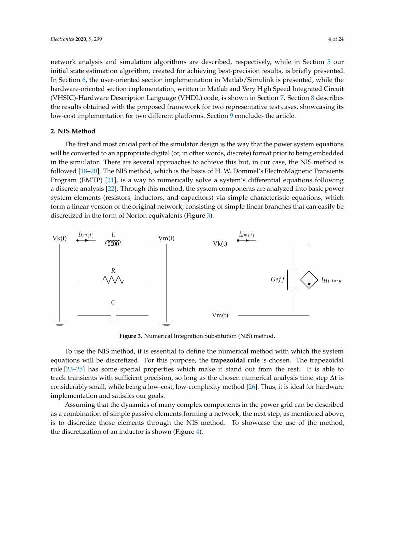
The first and most crucial part of the simulator design is the way that the power system equationswill be converted to an appropriate digital (or, in other words, discrete) format prior to being embeddedin the simulator. There are several approaches to achieve this but, in our case, the NIS method isfollowed [18–20]. The NIS method, which is the basis of H. W. Dommel’s ElectroMagnetic TransientsProgram (EMTP) [21], is a way to numerically solve a system’s differential equations followinga discrete analysis [22]. Through this method, the system components are analyzed into basic powersystem elements (resistors, inductors, and capacitors) via simple characteristic equations, whichform a linear version of the original network, consisting of simple linear branches that can easily bediscretized in the form of Norton equivalents (Figure 3).

Version January 20, 2020 submitted to Electronics 4 of 26

Figure 2. Logic diagram of the proposed framework

This article is organized as follows. In Section 2, the Numerical Integration Substitution106

(NIS) method, an essential technique in time-domain power system simulation, is presented,107

along with our custom optimizations and examples showcasing its use. In Sections 3 and108

4, the NIS-based network analysis and simulation algorithms are described, respectively,109

while in Section 5 our initial state estimation algorithm, created for achieving best-precision110

results, is briefly presented. In Section 6, the user-oriented section implementation in111

Matlab/Simulink is presented, while the hardware-oriented section implementation, written in112

Matlab and Very High Speed Integrated Circuit (VHSIC)-Hardware Description Language (VHDL)113

code, is shown in Section 7. Section 8 describes the results obtained with the proposed framework114

for two representative test cases , showcasing its low-cost implementation for 2 different platforms.115

Section 9 concludes the article.116

2. NIS method117

The first and most crucial part of the simulator design is the way that the power system118

equations will be converted to an appropriate digital (or, in other words, discrete) format prior119

to being embedded in the simulator. There are several approaches to achieve this but, in120

our case, the NIS method is followed [10], [12], [27]. The NIS method, which is the basis of121

Hermann W. Dommel’s ElectroMagnetic Transients Program (EMTP) [30], is a way to numerically122

solve a system’s differential equations following a discrete analysis [6]. Through this method ,123

the system components are analyzed into basic power system elements124

(resistors, inductors, capacitors) via simple characteristic equations, which form a linear version of the125

original network, consisting of simple linear branches that can easily be discretized in the form of126

Norton equivalents (Figure 3).127

ikm(t)Vk(t) Vm(t)L

R

C

Vm(t)

Vk(t)

ikm(t)

Ge f f IHistory

Figure 3. Numerical Integration Substitution (NIS) method

To use the NIS method, it is essential to define the numerical method with which the system128

equations will be discretized. For this purpose, trapezoidal rule is chosen. The trapezoidal rule [11],129

[28], [29] has some special properties which make it stand out from the rest. It is able to track transients130

Figure 3. Numerical Integration Substitution (NIS) method.

To use the NIS method, it is essential to define the numerical method with which the systemequations will be discretized. For this purpose, the trapezoidal rule is chosen. The trapezoidalrule [23–25] has some special properties which make it stand out from the rest. It is able totrack transients with sufficient precision, so long as the chosen numerical analysis time step ∆t isconsiderably small, while being a low-cost, low-complexity method [26]. Thus, it is ideal for hardwareimplementation and satisfies our goals.

Assuming that the dynamics of many complex components in the power grid can be describedas a combination of simple passive elements forming a network, the next step, as mentioned above,is to discretize those elements through the NIS method. To showcase the use of the method,the discretization of an inductor is shown (Figure 4).

Electronics 2020, 9, 299 5 of 24

Version January 20, 2020 submitted to Electronics 5 of 26

with sufficient precision, so long as the chosen numerical analysis time step ∆t is considerably small,131

while being a low-cost, low-complexity method [13] . Thus, it is ideal for hardware implementation132

and satisfies our goals.133

Assuming that the dynamics of many complex components in the power grid can be described134

as a combination of simple passive elements forming a network, the next step as mentioned above,135

is to discretize those elements through the NIS method. To showcase the use of the method, the136

discretization of an inductor is shown (Figure 4).137

+

−

Uk

ikm(t)

+

−

Um

Figure 4. Inductor

The behavior of the inductor is expressed by the following differential equation, with respect to138

Figure 4 notations:139

vL(t) = vk(t)− vm(t) = Ldikm(t)

dt

⇔ dikm(t)dt

=1L

vL(t)

⇔ ikm(t) = ikm(t− ∆t) +1L

∫ t

t−∆tvL(τ)dτ

Applying the trapezoidal rule yields:140

ikm(t) = ikm(t− ∆t) +∆t2L

[vL(t− ∆t) + vL(t)]

⇔ ikm(t) =∆t2L

vL(t) + [ikm(t− ∆t) +∆t2L

vL(t− ∆t)]

⇔ ikm(t) =∆t2L

[vk(t)− vm(t)]︸ ︷︷ ︸

Instantaneous term

+

{ikm(t− ∆t) +

∆t2L

[vk(t− ∆t)− vm(t− ∆t)]}

︸ ︷︷ ︸History term

(1)

As it has been explicitly clarified in equation 1, the characteristic equation of an inductor can141

be viewed as the sum of an instantaneous and a history term. The former describes the immediate142

response of the component to a change in the voltage difference across its terminals, while the latter143

represents an inherent memory of the component preventing the change of its state. Equation 1 can144

then be represented by a Norton equivalent, illustrated in Figure 5 [11], where the conductance G and145

the current source IHistory are the instantaneous and the history terms, respectively.146

Figure 4. Inductor.

The behavior of the inductor is expressed by the following differential equation, with respect tothe notation in Figure 4:

vL(t) = vk(t)− vm(t) = Ldikm(t)

dt

⇔ dikm(t)dt

=1L

vL(t)

⇔ ikm(t) = ikm(t− ∆t) +1L

∫ t

t−∆tvL(τ)dτ

Applying the trapezoidal rule yields:

ikm(t) = ikm(t− ∆t) +∆t2L

[vL(t− ∆t) + vL(t)]

⇔ ikm(t) =∆t2L

vL(t) + [ikm(t− ∆t) +∆t2L

vL(t− ∆t)] (1)

⇔ ikm(t) =∆t2L

[vk(t)− vm(t)]︸ ︷︷ ︸

Instantaneous term

+

{ikm(t− ∆t) +

∆t2L

[vk(t− ∆t)− vm(t− ∆t)]}

︸ ︷︷ ︸History term

As explicitly clarified in Equation (1), the characteristic equation of an inductor can be viewed asthe sum of an instantaneous term and a history term. The former describes the immediate response ofthe component to a change in the voltage difference across its terminals, while the latter representsan inherent memory of the component preventing the change of its state. Equation (1) can then berepresented by a Norton equivalent, as illustrated in Figure 5 [23], where the conductance G and thecurrent source IHistory are the instantaneous and the history terms, respectively.

Figure 5. Discrete model of the inductor.

Electronics 2020, 9, 299 6 of 24

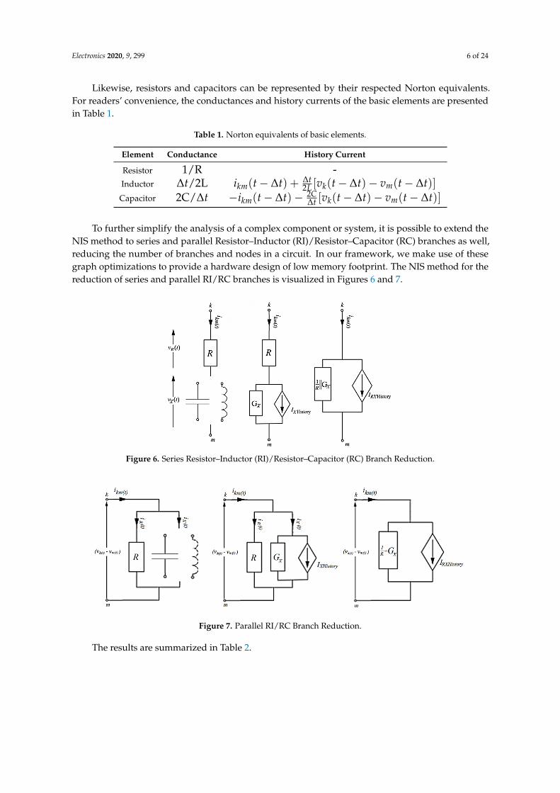
Likewise, resistors and capacitors can be represented by their respected Norton equivalents.For readers’ convenience, the conductances and history currents of the basic elements are presentedin Table 1.

Table 1. Norton equivalents of basic elements.

Element Conductance History Current

Resistor 1/R -Inductor ∆t/2L ikm(t− ∆t) + ∆t

2L [vk(t− ∆t)− vm(t− ∆t)]Capacitor 2C/∆t −ikm(t− ∆t)− 2C

∆t [vk(t− ∆t)− vm(t− ∆t)]

To further simplify the analysis of a complex component or system, it is possible to extend theNIS method to series and parallel Resistor–Inductor (RI)/Resistor–Capacitor (RC) branches as well,reducing the number of branches and nodes in a circuit. In our framework, we make use of thesegraph optimizations to provide a hardware design of low memory footprint. The NIS method for thereduction of series and parallel RI/RC branches is visualized in Figures 6 and 7.

Figure 6. Series Resistor–Inductor (RI)/Resistor–Capacitor (RC) Branch Reduction.

Figure 7. Parallel RI/RC Branch Reduction.

The results are summarized in Table 2.

Electronics 2020, 9, 299 7 of 24

Table 2. Norton equivalents of RI/RC branches.

Branch Type Conductance History Current

Series RIGL/R

1/R+GLGe f f [vk(t− ∆t)− vm(t− ∆t)] + Ge f f (Re f f − 2R)ikm(t− ∆t)

Series RCGC/R

1/R+GC−Ge f f [vk(t− ∆t)− vm(t− ∆t)]− Ge f f (Re f f − 2R)ikm(t− ∆t)

Parallel RI 1/R+GL (Ge f f − 2R )[vk(t− ∆t)− vm(t− ∆t)] + ikm(t− ∆t)

Parallel RC 1/R+GC −(Ge f f − 2R )[vk(t− ∆t)− vm(t− ∆t)]− ikm(t− ∆t)

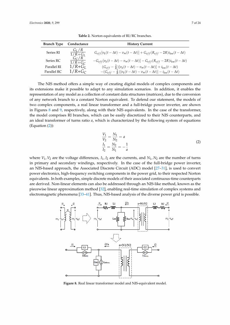
The NIS method offers a simple way of creating digital models of complex components andits extensions make it possible to adapt to any simulation scenarios. In addition, it enables therepresentation of any model as a collection of constant data structures (matrices), due to the conversionof any network branch to a constant Norton equivalent. To defend our statement, the models oftwo complex components, a real linear transformer and a full-bridge power inverter, are shownin Figures 8 and 9, respectively, along with their NIS equivalents. In the case of the transformer,the model comprises RI branches, which can be easily discretized to their NIS counterparts, andan ideal transformer of turns ratio a, which is characterized by the following system of equations(Equation (2)):

V1

V2=

N1

N2= a

I1

I2=

N2

N1= −1

a

(2)

where V1, V2 are the voltage differences, I1, I2 are the currents, and N1, N2 are the number of turnsin primary and secondary windings, respectively. In the case of the full-bridge power inverter,an NIS-based approach, the Associated Discrete Circuit (ADC) model [27–31], is used to convertpower electronics, high-frequency switching components in the power grid, to their respected Nortonequivalents. In both examples, simple discrete models of their associated continuous-time counterpartsare derived. Non-linear elements can also be addressed through an NIS-like method, known as thepiecewise linear approximation method [32], enabling real-time simulation of complex systems andelectromagnetic phenomena [33–41]. Thus, NIS-based analysis of the diverse power grid is possible.

Figure 8. Real linear transformer model and NIS-equivalent model.

Electronics 2020, 9, 299 8 of 24

Figure 9. Full bridge power inverter model and NIS analysis of power electronics using AssociatedDiscrete Circuit (ADC) model.

3. NIS-based Network Analysis Algorithm

After defining the NIS method, its use and extensions, a NIS-based network analysis algorithmis presented in this section. To simulate the given (micro)grid, there are three main steps to follow.The first step is to convert the grid into a form which can be discretized. As stated above, this canbe accomplished by modeling grid components as small networks of Resistor–Inductor–Capacitor(RIC) branches. Therefore, the whole grid can be discretized through NIS method in a simple manner.The second step is to collect the system equations and create a solvable mathematical problem.Having converted our study system into its NIS-based discretized form, which comprises conductancecomponents, current sources, and possibly voltage sources, the behavior of the system can be expressedin the form of:

Gvt = it + ItHistory (3)

where G is the conductance matrix, vt is the vector of nodal voltages at time step t, it is the vectorof external current sources at time step t, and It

History is the vector of history current sources at time stept. As stated in Section 2, the NIS method converts the system information to constant data structures, i.e.the G matrix, as well as the matrices of history current sources’ coefficients and branch conductances.In that way, complex systems comprising high-frequency switching components do not necessitatethe computation of different matrices associated with possible system topologies. The third step isto define the initial state of the system, which is addressed by our initial state estimation algorithmpresented in Section 5. In general, this process includes the initialization of history current sources andexternal sources and the computation of the system equations for t = 0+ (at the start of the simulation).In this way, we prevent possible simulation errors associated with zero state and zero input responsesof the system at t = 0+, when transient phenomena emerge.

To showcase the network analysis algorithm, a test circuit (Figure 10) is converted to its discretecounterpart (Figure 11) with the above process. The test circuit consists of a voltage source with itsinternal resistor, a single-phase linear transformer in its model form, a resistive load and two RCbranches. To analyze the network and transform it into Equation (3), the nodal analysis method isused. Having assigned id numbers to every node of the system, with the ground node being thereference node (V0 = 0V), and taking the component polarities into account, the process results in themathematical system shown in Figure 12. In this figure, the constant conductance matrix G is shownanalytically. It is worth mentioning that, to correctly transform the system into a mathematical equation,a property of the ideal transformer called mirroring effect is used. According to this, the impedance

Electronics 2020, 9, 299 9 of 24

seen from one side of the transformer is a mirror image of the impedance connected at the other side.Therefore, it is possible to shift branches from one side of the ideal transformer to the other withouterror, after applying some modifications first, as shown in Figure 13.

Figure 10. Test circuit to be analyzed by NIS-based network analysis algorithm.

Figure 11. Discrete version of the test circuit.

Figure 12. Test circuit in the form of Equation (3).

Figure 13. Secondary side branch of ideal transformer referred to the primary.

Electronics 2020, 9, 299 10 of 24

4. NIS-based Simulation Algorithm

After employing the NIS-based network analysis algorithm, the simulation algorithm follows.The first step is the computation of the new values of the external sources and the history currentsources, using the equations derived from the NIS method. The second step is the computation of thenodal voltages. From Equation (3):

vt = G−1(it + ItHistory) (4)

where G−1 is the inverse conductance (resistance) matrix, which (for a given network topology) isconstant throughout the simulation and needs to be calculated only once. In the case of voltage sourcesexisting in the network, the process slightly changes. Equation (3) is rewritten in the form:

[GUU GUKGKU GKK

] [vt

uvt

k

]=

[itu

itk

]+

[ItUHistory

ItKHistory

](5)

where matrix G is divided into four submatrices, each with a different subscript set, and thevoltage/current vectors are divided into two subvectors. The subscripts U and K represent connectionsto nodes with unknown and known voltages, respectively. Then, Equation (5) is transformed intoEquation (6), which returns the unknown nodal voltages’ values:

GUUvtU = it

U + ItUHistory − GUKvt

K = (itU)′

⇔ vtU = G−1

UU(itU)′

(6)

Equivalently, the currents of voltage sources are given by Equation (7):

GKUvtU + GKKvt

K = itK + It

KHistory

⇔ itK = GKUvt

U + GKKvtK − It

KHistory (7)

The third step is to compute all the branch currents of the network at the present time step. This isdue to the fact that the branch currents constitute valuable information about the network, since theyare essential to the computation of the values of the history current sources at next time step. Knowingthe conductance of the branches, the computation of the values of the history current sources andnodal voltages is a simple task. After the completion of these steps, the simulation cycle restarts untilthe predefined stop time.

It is worth noting that, in our design, the computation of the inverse matrices of the aboveequations is handled by the Singular Value Decomposition (SVD) method [42]. This method canbe used to approximate the inverse of any conductance matrix G, even if it is ill-conditioned (itsdeterminant is close to zero), which is essential for the simulation of many different systems.

5. Initial State Estimation Algorithm

In typical system simulation programs such as Simulink, during the configuration of the studysystem design and simulation parameters, an internal initial system state is defined. At the beginning ofthe simulation, at t = 0+, the network is stimulated by external sources in an instant, such as turningon multiple switches simultaneously, therefore connecting the sources to the grid. During this process,the system is undergoing a transient state. That is, the initial conditions affect the system state after thevery first time step. This is due to the rapid changes the system experiences from the “switching” effect.

To cope with this problem, a review in basic electrical circuit theory is mandatory. The “memory”components, the inductor and the capacitor, resist the sudden changes of their current and voltage,respectively. When a given system has an initial state before its stimulation by the sources, whichmeans that the capacitors and inductors of the network have some initial voltage and current prior to

Electronics 2020, 9, 299 11 of 24

their excitation, respectively, it shows some starting “inertia”. To solve this problem and be precise,during the first time step (t = 0+), it is suggested that all inductors be substituted by current sources ofvalues equal to the initial currents. In the same way, all capacitors should be substituted by voltagesources of values equal to the initial voltages. The general concept is shown in an example in Figure 14.For zero initial state only, inductors can be thought as being open circuits whereas capacitors asshort circuits. Having those facts in mind, the system under study can be reformed to its initial-stateconfiguration and be solved afterwards with the help of the preestablished process (Equations (4), (6),(7)). After that, the analysis resumes in the standard way.

Figure 14. Initial state model.

This methodology, called the initial state estimation algorithm, is an important asset to ourframework, providing best-precision simulation results in any study case. The initial state derived bythis algorithm is used below as the default starting point of the hardware simulator.

6. User-Oriented Section

Having covered the basic theoretical concepts for real-time power system simulation, ourprototype implementation of an automatic design framework is presented here. The first part ofour implementation is the user-oriented section. This section is dedicated to the user, the electricalor future smart grid engineer, providing tools and algorithms needed to draw a schematic, testa component model, and convert the schematic to a structure compatible with an HDL template. Thereare plenty of software tools and specialized libraries that can offer some of the capabilities needed forthis section. In the context of this first attempt to design the framework and prove its functionality,we have chosen to work with existing software suites providing some basic GUI. One of the mostknown software suites that supports our needs regarding the design of the application architecture andprovides numerous tutorials and educational documentation is Matlab. Matlab is an all-in-one solutionthat supports a wide variety of engineering problems and is widely spread across the academia [43].Its simulation package, Simulink, is assumed to be very accurate, up-to-date, and supports problemsof any kind, from fluid dynamics to electrical engineering [44].

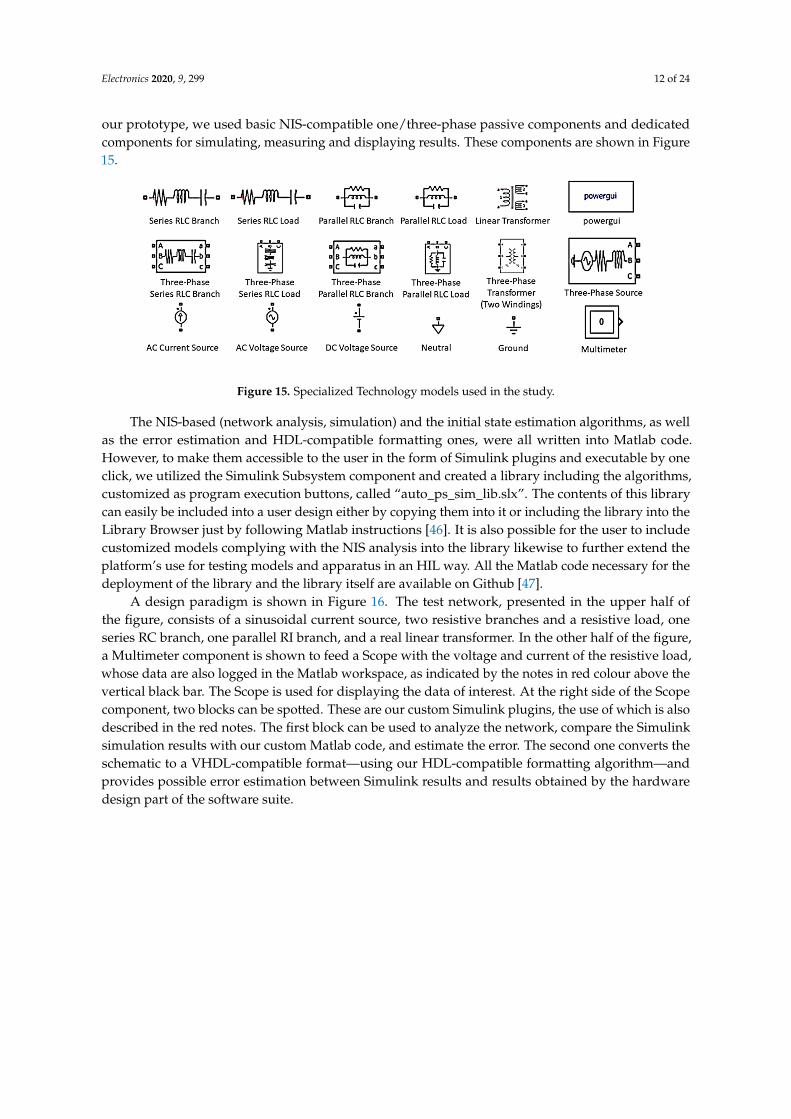
In the context of our proposed framework, the concept was to make use of the Simulink GUIand a library called Simscape and create our custom Matlab code which reads the user’s input,the schematic of the system, and automatically extracts the required information to provide the neededservices. The Simulink GUI consists of many simulation tools and functions, the most importanttools of which—those used in the analysis—are the Model Configuration Parameters and the LibraryBrowser. The Model Configuration Parameters, on the one hand, is the tool with which the simulationtime and the Simulink solver options, needed for the model error estimation, are set. The LibraryBrowser, on the other hand, is a (browser) tool providing access to all the Simulink libraries, includingthe Simscape library. The Simscape library includes a dedicated library for power systems calledSpecialized Technology [45], which features specialized power system models and enables an interfacewith other Simulink tools in a simple manner, creating a strong interconnection between Matlaband Simulink. Therefore, to achieve design simplicity and use up-to-date models, we opted forthe Specialized Technology library and its models to be in the user-oriented section design. For

Electronics 2020, 9, 299 12 of 24

our prototype, we used basic NIS-compatible one/three-phase passive components and dedicatedcomponents for simulating, measuring and displaying results. These components are shown in Figure15.

Figure 15. Specialized Technology models used in the study.

The NIS-based (network analysis, simulation) and the initial state estimation algorithms, as wellas the error estimation and HDL-compatible formatting ones, were all written into Matlab code.However, to make them accessible to the user in the form of Simulink plugins and executable by oneclick, we utilized the Simulink Subsystem component and created a library including the algorithms,customized as program execution buttons, called “auto_ps_sim_lib.slx”. The contents of this librarycan easily be included into a user design either by copying them into it or including the library into theLibrary Browser just by following Matlab instructions [46]. It is also possible for the user to includecustomized models complying with the NIS analysis into the library likewise to further extend theplatform’s use for testing models and apparatus in an HIL way. All the Matlab code necessary for thedeployment of the library and the library itself are available on Github [47].

A design paradigm is shown in Figure 16. The test network, presented in the upper half ofthe figure, consists of a sinusoidal current source, two resistive branches and a resistive load, oneseries RC branch, one parallel RI branch, and a real linear transformer. In the other half of the figure,a Multimeter component is shown to feed a Scope with the voltage and current of the resistive load,whose data are also logged in the Matlab workspace, as indicated by the notes in red colour above thevertical black bar. The Scope is used for displaying the data of interest. At the right side of the Scopecomponent, two blocks can be spotted. These are our custom Simulink plugins, the use of which is alsodescribed in the red notes. The first block can be used to analyze the network, compare the Simulinksimulation results with our custom Matlab code, and estimate the error. The second one converts theschematic to a VHDL-compatible format—using our HDL-compatible formatting algorithm—andprovides possible error estimation between Simulink results and results obtained by the hardwaredesign part of the software suite.

Electronics 2020, 9, 299 13 of 24

Figure 16. Test network designed in Simulink General User Interface (GUI); important details and toolsare marked in red.

7. Hardware-Oriented Section

The second part of our implementation is the hardware-oriented section. This section focuses onthe actions that must be made for a study case to be embedded in an FPGA and run in real-time, whileusing minimum computational resources and memory. Taking into account the user’s specifications,this section acts as an interface between the user and the hardware implementation, removing anyneed for previous knowledge of HDLs from the user. It comprises two major modules: a modulewhich helps the user specify a fixed-point data representation for the custom real-time hardwaresimulator and an HDL template which converts the schematic into a dedicated hardware architecture.In our prototype, we deployed the Fixed-Point Converter tool of Matlab [48] for the former module’simplementation, while the latter used our VHDL-compatible formatting algorithm and a VHDLtemplate for the actual automatic hardware design.

To design an efficient hardware architecture, one crucial aspect is memory footprint, which affectsgreatly the power consumption of a chip. When dealing with hard computational problems, suchas the precise simulation of a system’s behavior after a sequence of specific events, memory playsan important role. This is due to the number of memory cells, registers, flip-flops, etc. needed to achievethe problem-defined numerical accuracy. The number of bits in a digital design is not infinite, so as towithstand any numerical accuracy problem, nor can it cover a very wide range. In most cases, register sizeis constant throughout a design. This fixed bit length of digital values, while creating a consistent design,also minimizes power consumption due to reduced utilized hardware resources. In addition, numericalcomputations with fixed length and fixed data representation need less time than floating-point ones. Thus,creating an efficient simulator design calls for a global digital data representation, sufficient—accordingto the user—and in the same time small enough to limit power consumption.

In that respect, the Fixed-Point Converter tool of Matlab is a simple yet effective way for choosingthe optimal fixed-point data representation. This tool is given the necessary computational tasks asinputs (in the form of functions), along with the network analysis and simulation script. Then, afterspecifying the fixed-point analysis properties, the tool runs the whole script and proposes fixed-pointdata representations for all the task variables. After choosing a global data representation with thehelp of the tool (by inspecting the range of the results), the tasks are converted into their fixed-pointcounterparts. The numerical accuracy of the fixed-point tasks can be tested either by the tool itself or byintegrating the tasks within the network analysis and simulation script to create a fixed-point one forpre-implementation, and simulation purposes. Prior to the fixed-point analysis, a word length should

Electronics 2020, 9, 299 14 of 24

be specified and data should be declared as signed data or else wrong hardware implementation willbe derived. A sample configuration and fixed-point analysis results are shown in Figures 17 and 18,respectively. In the latter figure, the “.m” files on the left are the tasks and the emts_FP.m testbench fileis a copy of the network analysis and simulation script for fixed-point analysis purposes only.

Figure 17. Fixed-Point Converter Sample Configuration.

Figure 18. Fixed-Point analysis results.

To be able to convert the information of a study system in a VHDL-compatible format, a dedicatedscript calls the network analysis algorithm to read and analyze the schematic, while applying graphoptimizations, asks the user for the desired fixed-point properties (word and fraction length) andexports the network’s information in specific text files, coded in the desired binary format. All theimportant constant matrices or vectors (G−1, history current coefficients, and branch conductances)follow the user’s specifications, while some information matrices about network connections or numberof nodes/voltage (current) sources/fixed-point parameters are coded differently, since their purpose isto be used in the VHDL template only for information reasons. This script is deployed through theSimulink GUI as a plugin, as shown in Figure 16.

Electronics 2020, 9, 299 15 of 24

To be able to design a custom hardware architecture automatically for a power system simulator,our VHDL template is employed, which maps any power system simulator information to a predefined,customized, yet configurable hardware design. This hardware design can be viewed in Figure 19in a block diagram form. It consists of five modules: the History Currents module computes thehistory current sources’ values, the Nodal Currents module computes the vector of currents needed inEquation (4), the Nodal Voltages module solves Equation (4), the Branch Voltages module transformsnodal to branch voltages, and the Branch Currents module computes the branch currents’ values.

Figure 19. Top-level block diagram of a power system hardware simulator.

Each module is designed to be extensible and adaptive to any study case. To achieve this inVHDL [49–51], which is a powerful, yet stiff hardware description language, our template consists ofdedicated VHDL packages and functions to simplify the design and achieve the required flexibility.An important factor of the design is the Matlab-generated text files. When the template is synthesizedvia hardware design tools for a netlist to be created, the first step is for the text files to be read. Then,the network information is passed to the tools and can be used for appropriate design decisions.These decisions take place inside each module and are witnessed in the form of generated hardware.For example, let us focus on the case of “Nodal Voltages” module, where Equation (4) is solved. Asshown in Figure 20, for an arbitrary network, each nodal voltage in the “Nodal Voltages” module iscomputed by a dedicated datapath associated with its mathematical expression. Our template ensuresthat no unused computations will occupy hardware resources (e.g., for multiplications/additions withzero elements) and that the datapath will not feature unnecessary processing stages that add delay to thecomputations.

The VHDL-compatible formatting algorithm can be found in the user-oriented section folder atGithub [47], while the VHDL template is in the hardware-oriented section folder. Implementationinstructions can be found online.

Electronics 2020, 9, 299 16 of 24

Figure 20. Conversion of equations to hardware architecture.

8. Results

8.1. First Test Case

8.1.1. Simulation

For the first test case, the Simulink model shown in Figure 16, analyzed in Section 6, was used asinput to the Simulink GUI. For an analysis time step, we used ∆t = 50 µs, a relatively standard one foreffectively capturing transient phenomena in power systems. Firstly, we simulated the model via theSimulink mathematical algorithms and the NIS method using double-precision (Matlab) operations.The purpose of this action was to test the NIS method prior to hardware implementation. To estimatethe NIS method’s error, the voltage and current values of the network’s resistive load, derived by NISmethod, were compared to the Simulink results. The results are shown in Figure 21 below:

It can be easily derived that all the NIS-based algorithms and the component models used areimplemented in the right way, as the error is close to zero.

After the system’s conversion to VHDL code with 34 bits word length and 19 bits fraction length(as dictated by the corresponding bit length estimation tool of our framework), the system wassimulated using Vivado and ISE tools (hardware design software suites) with target devices the ZyboZ7-20 and the Virtex 6 ML605 Evaluation board, respectively. After collecting all the voltage andcurrent values of the network’s resistive load from the corresponding tools in fixed-point format,the error was computed by comparing these results with the Simulink ones. The computation errorsare shown in Figure 22.

Electronics 2020, 9, 299 17 of 24

Figure 21. Simulink-NIS method error results.

Figure 22. Simulink-hardware error results.

The figure showcases the impact of the user-specified word length in the simulator’s accuracy.Depending on the system simulation requirements, the word length and the results’ accuracy may vary.Overall, the error results are acceptable as being below zero and can be further restricted according tothe user’s wishes.

8.1.2. Hardware Design

As mentioned above, the hardware implementation of the first test case was successfully deployedin Virtex 6 ML605 Evaluation board [52], as well as in Zybo Z7-20 device [53]. An image of theimplementation in Virtex 6’s FPGA is shown in Figure 23. In this image, the mapping of the physicalhardware instances on the FPGA is indicated by the blue color.

Electronics 2020, 9, 299 18 of 24

Figure 23. FPGA mapping of the first test case simulator.

The utilization results of the hardware design in Zybo Z7-20 and Virtex 6 ML605 Evaluation boardare shown in Table 3.

Table 3. Utilization results.

Board Site Type Used Available Util%

Slice LUTs 4055 53,200 7.62Zybo Z7-20 board (xc7z020clg400-1) Slice Registers 494 106,400 0.46

DSPs (DSP48E1 only) 58 220 26.36

Slice LUTs 1991 46,560 4Virtex 6 ML605 Evaluation board (xc6vlx75t-1-ff484) Slice Registers 459 93,120 0

DSPs (DSP48E1 only) 98 288 34

In both cases, the implementation of the network simulation, by the proposed framework, resultsin a low-cost hardware design of low computational resources and memory usage. It is interesting tonotice that, even in the case of Zybo Z7-20 board, which uses a smaller FPGA, the results show loweruse of Digital Signal Processing (DSP) modules, resulting in a more efficient design.

In addition, the timing summary of the hardware designs in Table 3 is presented in Table 4.

Table 4. Timing summary.

Board Max Frequency Max Throughput Max Latency

Zybo Z7-20 board (xc7z020clg400-1) 30.212 MHz 30.212 Msampless

∗33.10 ns

Virtex 6 ML605 Evaluation board (xc6vlx75t-1-ff484) 32.755 MHz 32.755 Msampless

∗30.53 ns

* Assuming the hardware simulator outputs one sample per clock cycle.

Electronics 2020, 9, 299 19 of 24

The results show that, in both cases, the designs for both target (FPGA) devices achieve latencyclose to 30 ns, maximum throughput of around 33 Msamples per second for an output of one sample,and operational frequency close to 33 MHz. This means that, for an analysis time step equal to ∆t = 50µs,which tracks effectively the transients of a system, our hardware simulator is able to make an almost30-min analysis of a simple microgrid-size circuit in 1 s, thus meeting network’s real-time requirements.

8.2. Second Test Case

8.2.1. Simulation

For the second test case, the Simulink model shown in Figure 24 was used as input to theSimulink GUI. This model is a variant of a typical Institute of Electrical and Electronics Engineers(IEEE) 5-Bus Model. It consists of two three-phase current sources, seven pi-modeled transmissionlines, and four three-phase RI loads. For the analysis time step, we used ∆t = 50 µs, as in the previousscenario. Firstly, we simulated the Simulink mathematical algorithms and the NIS method usingdouble-precision Matlab operations. To estimate the NIS method’s error, the voltage and current valuesof LOAD 5, derived by NIS method, were compared to the Simulink ones. The results are shownin Figure 25.

It can be easily derived that all the NIS-based algorithms and the component models used areimplemented in the right way, as the error is close to zero.

After the system’s conversion to VHDL code with 34 bits word length and 19 bits fraction lengthagain, the system was simulated by Vivado and ISE tools for the Zybo Z7-20 and Virtex 6 ML605Evaluation board, respectively. After collecting all the voltage and current values of the network’sLOAD 5 in fixed-point format, the error was computed by comparing these results with the Simulinkones. The computation errors are shown in Figure 26.

Figure 24. Simulink model of the second test scenario.

Electronics 2020, 9, 299 20 of 24

Figure 25. Simulink-NIS method error results for second test scenario.

Figure 26. Simulink-hardware error results for second test scenario.

It is obvious that the figures’ waveforms are matching, with the only difference being the slightlydifferent accuracies of the results.

8.2.2. Hardware Design

The utilization results of the hardware design in Zybo Z7-20 and Virtex 6 ML605 Evaluation boardare shown in Table 5.

In both target devices, and as in the first test case, the implementation of the network simulationfits perfectly inside the FPGAs. Again, it could be noted that, in the case of Zybo Z7-20 board, equippedwith a smaller size FPGA device (compared to the Virtex 6 device), we have much lower utilization ofthe DSP modules, thus indicating that in this test case too, Zybo handles more efficiently DSP designs.

In addition, the timing summary of the hardware designs in Table 5 is presented in Table 6.

Electronics 2020, 9, 299 21 of 24

Table 5. Utilization results.

Board Site Type Used Available Util%

Slice LUTs 42,862 53,200 80.57Zybo Z7-20 board (xc7z020clg400-1) Slice Registers 3570 106,400 3.36

DSPs (DSP48E1 only) 96 220 43.64

Slice LUTs 40,452 46,560 86Virtex 6 ML605 Evaluation board (xc6vlx75t-1-ff484) Slice Registers 3264 93,120 3

DSPs (DSP48E1 only) 288 288 100

Table 6. Timing summary.

Board Max Frequency Max Throughput Max Latency

Zybo Z7-20 board (xc7z020clg400-1) 29.607 MHz 29.607 Msampless

∗33.78 ns

Virtex 6 ML605 Evaluation board (xc6vlx75t-1-ff484) 33.102 MHz 33.102 Msampless

∗30.21 ns

* Assuming the hardware simulator outputs one sample per clock cycle.

Using a similar analysis as in the previous test case, it can be easily derived from Table 6 thatnetwork’s real time requirements associated with this test case are also met.

9. Discussion

As stated in the Introduction, our work is a first attempt to create a full-solution platform thatprovides a simple, yet easy to use framework, featuring tools for drawing power systems and designingcomponent models, while enabling simulations directly on hardware. It is designed for targetingmainly microgrid systems on FPGA platforms so as to make use of their reconfigurable characteristicsand their inherent resources’ parallelism, to be able to create efficient hardware implementations onthe same (low cost) device (Zybo Z7-20 is an indicative paradigm of such a low cost device), thussaving costs, especially since, as demonstrated through the test cases, a migrogrid-like structure canbe readily accommodated in an FPGA device with low-medium resources such as the Zybo Z7-20one. In addition, it is also compatible with many well known industry standard hardware designtools, such as Vivado and other platforms supporting the VHDL-93 standard. Therefore, it can beextended to target multiple FPGA devices as well. Moreover, this framework is the first step towardsour open source platform vision, which will enable the design of smart (micro)grid-related applicationsand their implementation in real scenarios, outside of the laboratory, in low-cost FPGA platforms(especially when microgrids are involved, which is the current target of our framework), providingan accessible solution for smart grid researchers without the need of buying licenses for proprietaryproducts. Beyond this, due to the high timing scores achieved and the real-time performance of thededicated hardware, it can be easily deduced that smart (micro)grid applications requiring real-timesimulation (computing) capabilities can be addressed without suffering from computation overheads.

Future work will be dedicated to the inclusion of more power system electronics’ models as wellas non-linear elements in the framework. Next, further research will address the automatic hardwareimplementation, in the sense of how it can become more efficient while continuing to achieve lowimplementation cost and high performance. Moreover, a complete open source user-oriented sectionwill be designed to promote the framework’s use and access so as to lead towards a fully open sourceplatform. Finally, to fully utilize the hardware simulator and extend its use, standard interfaces couldbe designed for SoC-embedded system applications.

Author Contributions: Conceptualization, E.M., N.T., M.B., and A.B.; Data curation, E.M. and N.T.; Formalanalysis, E.M. and N.T.; Investigation, E.M. and N.T.; Methodology, E.M., N.T., M.B., and A.B.; Projectadministration, M.B. and A.B.; Resources, M.B. and A.B.; Software, E.M. and N.T.; Validation, E.M. and N.T.;Visualization, E.M.; Writing—original draft, E.M.; and Writing—review and editing, M.B. and A.B. All authorshave read and agreed to the published version of the manuscript.

Electronics 2020, 9, 299 22 of 24

Funding: The work of A. Birbas and N. Tzanis was partially co-funded by E.U and national funds the RegionalOperation Programme “Western Greece 2014–2020” under the RIS3 Programme in “Microelectronics and SmartMaterials” (Project: FPGAs 4SGs-MIS: 5021446). The work of M. Birbas and E. Mylonas was partially co-fundedby E.U and national funds the Regional Operation Programme “Western Greece 2014–2020” under the RIS3Programme in “Microelectronics and Smart Materials” (Project: DEEP-EVIoT-MIS: 5038640).

Conflicts of Interest: The authors declare no conflict of interest.

Abbreviations

The following abbreviations are used in this manuscript:FPGA Field Programmable Gate ArrayVHSIC Very High Speed Integrated CircuitVHDL VHSIC-Hardware Description LanguageRES Renewable Energy SourceDER Distributed Energy ResourceAI Artificial IntelligenceLEM Local Energy MarketIoT Internet of ThingsML Machine LearningGPGPU General-Purpose Graphics Processing UnitGUI General User InterfaceHDL Hardware Description LanguageHIL Hardware-In-the-LoopNIS Numerical Integration SubstitutionEMTP ElectroMagnetic Transients ProgramRI Resistor–InductorRC Resistor–CapacitorADC Associated Discrete CircuitRIC Resistor–Inductor–CapacitorSVD Singular Value DecompositionDSP Digital Signal ProcessingIEEE Institute of Electrical and Electronics Engineers

References

1. What Is the Smart Grid? Available online: https://www.smartgrid.gov/the_smart_grid/smart_grid.html(accessed on 3 September 2019).

2. Thierry Legrand, La Numérisation de L’énergie (4/4): La RéVolution Industrielle des Smart Grids. Availableonline: https://les-smartgrids.fr/numerisation-energie-revolution-smart-grids (accessed on 2 July 2019).

3. Chai, B.; Chen, J.; Yang, Z.; Zhang, Y. Demand Response Management With Multiple Utility Companies:A Two-Level Game Approach. IEEE Trans. Smart Grid 2014, 5, 722–731. [CrossRef]

4. Apostolopoulos, P.A.; Tsiropoulou, E.E.; Papavassiliou, S. Demand Response Management in Smart GridNetworks: A Two-Stage Game-Theoretic Learning-Based Approach. Mobile Netw. Appl. 2018. [CrossRef]

5. Kabalci, Y. A survey on smart metering and smart grid communication. Renew. Sustain. Energy Rev. 2016, 57,302–318. [CrossRef]

6. Watson, N.R.; Arrillaga, J. Power systems electromagnetic transients simulation. IEEE Power Energy 2003,39, 449.

7. Anaya-Lara, O.; Acha, E. Modeling and Analysis of Custom Power Systems by PSCAD/EMTDC. IEEE Trans.Power Deliv. 2002, 17, 266–272. [CrossRef]

8. Zahavir, J.M.; krillaga, J.; Watson, N.R. Hybrid electromagnetic transient simulation with the state variablerepresentation of HVDC converter plant. IEEE Trans. Power Deliv. 1993, 8, 1591–1598. [CrossRef]

9. Durie, R.C.; Pottle, C. An extensible real-time digital transient network analyzer. IEEE Trans. Power Syst.1993, 8, 84–89. [CrossRef]

10. OPAL-RT Technologies, eFPGASIM. Available online: https://www.opal-rt.com/systems-efpgasim(accessed on 12 January 2020).

Electronics 2020, 9, 299 23 of 24

11. Typhoon HIL. Available online: https://www.typhoon-hil.com (accessed on 12 January 2020).12. Dommel, H.W. Digital Computer Solution of Electromagnetic Transients in Single-and Multiphase Networks.

IEEE Trans. Power Appar. Syst. 1969, 88, 388–399. [CrossRef]13. Farzanehrafat, A. Power Quality State Estimation. Ph.D. Dissertation, University of Canterbury, Christchurch,

New Zealand, 2014.14. Mahseredjian, J. Computation of Power System Transients: Overview and Challenges. In Proceedings of the

IEEE Power Engineering Society General Meeting, Tampa, FL, USA, 24–28 June 2007.15. Woods, R.; Mcallister, J.; Turner, R.; Yi, Y.; Lightbody, G. FPGA-Based Implementation of Signal Processing

Systems; Wiley: Hoboken, NJ, USA, 2008.16. Chen, Y.; Dinavahi, V. FPGA-Based Real-Time EMTP. IEEE IEEE Trans. Power Deliv. 2009, 24, 892–902.

[CrossRef]17. Parma, G.G.; Dinavahi, V. Real-time digital hardware simulation of power electronics and drives. IEEE Trans.

Power Deliv. 2007, 22, 1235–1246. [CrossRef]18. Dommel, H.W. Electromagnetic Transients Program Theory Book; Bonneville Power Administration: Portland,

OR, USA, 1986.19. Matar, M.; Bayoumi, A.M. An FPGA-Based Real-Time Simulator for the Analysis of Electromagnetic

Transients in Electrical Power Systems. Ph.D. Dissertation, University of Toronto, Toronto, ON, Canada, 2009.20. Manitoba HVDC Research Center Inc. EMTDC User’s Guide; Manitoba HVDC Research Center Inc.: Winnipig,

MB, Canada, 2004.21. Dommel, H.W. EMTP Theory Book; Microtran Power System Analysis Corporation: Vancouver, BC,

Canada, 1996.22. Bari, A.; Jiang, J.; Saad, W.; Arunita, J. Challenges in the Smart Grid Applications: An Overview. Int. J.

Distrib. Sens. Netw. 2014, 1–11. [CrossRef]23. Hollman, J.A. Step by Step Eigenvalue Analysis with EMTP Discrete Time Solutions New Methodology Test Cases;

The University of British Columbia: Vancouver, BC, USA, 2006.24. Hall, G.; Watt, J. Modern Numerical Methods for Ordinary Differential Equations; Oxford University Press:

New York, NY, USA, 1976.25. Selhi, H.; Christopoulos, C. Generalised TLM Switch Model for Power Electronics Applications. IEEE Proc.

Sci. Meas. Technol. 1998, 145, 101–104. [CrossRef]26. Razzaghi, R.; Mitjans, M.; Rachidi, F.; Paolone, M. An automated FPGA real-time simulator for power

electronics and power systems electromagnetic transient applications. Electr. Power Syst. Res. 2016, 141,147–156. [CrossRef]

27. Hui, S.Y.R.; Morrall, S. Generalised associated discrete circuit model for switching devices. IEEE Proc. Sci.Meas. Technol. 1994, 141, 57–64. [CrossRef]

28. Tzanis, N.; Andriopoulos, N.; Proiskos, G.; Birbas, M.; Birbas, A.; Housos, E. Computationally EfficientRepresentation of Energy Grid-Cyber Physical System. In Proceedings of the IEEE Industrial Cyber-PhysicalSystems (ICPS), St. Petersburg, Russia, 15–18 May 2018.

29. Tzanis N.; Proiskos G.; Birbas M.; Birbas A. FPGA-Assisted Distribution Grid Simulator. In Proceedings ofthe ARC 2018 Conference, Santorini, Greece, 8 April 2018.

30. Marti, J.R.; Lin, J. Suppression of Numerical Oscillations in the EMTP. IEEE Trans. Power Syst. 1989, 9, 71–72.[CrossRef]

31. Gear, C.W. Numerical Initial Value Problems in Ordinary Differential; Prentice Hall: Upper Saddle River, NJ,USA, 1971.

32. Escamilla, A.C. Modelling Non-linear and Distributed Elements in Transient State Estimation.Ph.D. Dissertation, University of Canterbury, Christchurch, New Zealand, 2015.

33. Marti, J.R.; Linares, L.R. Real-time EMTP-based Transients Simulation. IEEE Trans. Power Syst. 1994, 9,1309–1317. [CrossRef]

34. Sybille, G.; Giroux, P. Simulation of FACTS Controllers Using the MATLAB Power System Blockset andHypersim Real-time Simulator. In Proceedings of the IEEE Power Engineering Society Winter Meeting,New York, NY, USA, 27–31 January 2002.

35. Devaux, O.; Levacher, L.; Huet, O. An Advanced and Powerful Real-time Digital. IEEE Trans. Power Deliv.1998, 13, 421–426. [CrossRef]

Electronics 2020, 9, 299 24 of 24

36. Pak, L.; Faruque, M.O.; Nie, X.; Dinavahi, V. A Versatile Cluster-based Realtime Digital Simulator for PowerEngineering Research. IEEE Trans. Power Syst. 2006, 21, 455–465. [CrossRef]

37. Hollman, J.A.; Marti, J.R. Real Time Network Simulation with PC-Cluster. IEEE Trans. Power Syst. 2003, 18,563–569. [CrossRef]

38. Kuffel, R.; Beum, Y.; Lee, J. Overview of the Development and Installation of KEPCO Enhanced PowerSystem Simulator. In Proceedings of the 2000 IEEE Power Engineering Society Winter Meeting, Vasteras,Sweden, 23–27 January 2000.

39. Abourida, S.; Belanger, J.; Dufour, C. Real-Time HIL Simulation of a Complete PMSM Drive at 10’s TimeStep. In Proceedings of the 11th European Conference on Power Electronics and Applications, Dresden,Germany, 11–14 September 2005.

40. Dinavahi, V. Real-Time Digital Simulation of Switching Power Circuits. Ph.D. Dissertation, University ofToronto, Toronto, ON, Canada, 2000.

41. Strunz, K. Flexible Numerical Integration for Efficient Representation of Switching in Real TimeElectromagnetic Transients Simulation. IEEE Trans. Power Deliv. 2004, 19, 1276–1283. [CrossRef]

42. Jia, Y.-B. Singular Value Decomposition. 2013. Available online: http://web.cs.iastate.edu/~cs577/handouts/svd.pdf (accessed on 30 November 2019).

43. The Math Works Inc. Matlab Optimization Toolbox—User’s Guide. Available online: https://www.mathworks.com/help/pdf_doc/optim/optim_tb.pdf (accessed on 4 August 2019).

44. The Math Works Inc. Simulink—Getting Started Guide. Available online: https://www.mathworks.com/help/pdf_doc/simulink/sl_gs.pdf (accessed on 4 August 2019).

45. The Math Works Inc. Simscape Electrical—User’s Guide (Specialized Power Systems). Available online:https://www.mathworks.com/help/pdf_doc/physmod/sps/powersys.pdf (accessed on 26 July 2019).

46. The Math Works Inc. Add Libraries to the Library Browser. Available online: https://www.mathworks.com/help/simulink/ug/adding-libraries-to-the-library-browser.html (accessed on 20 November 2019).

47. Auto Design Framework for Real-time Power System Simulators. Available online: https://github.com/lefmylonas/auto_power_system_simulator.git (accessed on 7 January 2020).

48. The Math Works Inc. Fixed-Point Designer—User’s Guide. Available online: https://www.mathworks.com/help/pdf_doc/fixedpoint/FPTUG.pdf (accessed on 7 August 2019).

49. Armstrong, J.R.; Gray, F.G. VHDL Design Representation and Synthesis, 2nd ed.; Prentice Hall PTR:Upper Saddle River, NJ, USA, 2000.

50. Pellerin, D.; Taylor, D. VHDL Made Easy; Prentice Hall: Upper Saddle River, NJ, USA, 1997.51. Vahid, F. VHDL for Digital Design; John Wiley & Sons: Hoboken, NJ, USA, 2007.52. ML605 Hardware User Guide, UG534 (v1.9). 26 February 2019. Available online: https://www.xilinx.com/

support/documentation/boards_and_kits/ug534.pdf (accessed on 15 October 2019).53. Zybo Z7 Board Reference Manual, Revised 21 February 2018. Available online: https://reference.digilentinc.

com/_media/reference/programmable-logic/zybo-z7/zybo-z7_rm.pdf (accessed on 12 October 2019).

c© 2020 by the authors. Licensee MDPI, Basel, Switzerland. This article is an open accessarticle distributed under the terms and conditions of the Creative Commons Attribution(CC BY) license (http://creativecommons.org/licenses/by/4.0/).