ED302_2012_DOE&Anova

2/1/2012

1

ED 302. Design for XJan –Apr 2012

Instructor: Palani Ramu

2/1/2012 ED 302. [email protected] 1

DFSS- Phases

P1: Identify requirements Project charter, Customer requirements

P2: Characterize design Translate customer requirements, design alternatives: DFX, DFMEA,

CAD/CAE

Optimize the design DOE, Simulation tools, Taguchi method, tolerance design, robust- reliability

based design

Validate the design


DOE, Reliability testing, confidence analysis

2/1/2012

2

Experiments (DOE)

DOE serve two purpose:

Get the statistics of a response ( how the product or process performs)

Come up with a Transfer function that can be used for further engineering analysis like parameter


optimization or tolerance analysis ( What are the parameters that influence the outcome)

Language of experiments

Factor (inputs, causes, parameters, ingredients) Anything that is suspected to have an influence on the performance

of the product. Can control/adjust Continuous factor (ex: temperature, time) Discrete factor (ex: machine brand, tool type, material)

Level Value or status that factor holds within an experiment Temperature –factor, 200deg, 300 deg Levels


Result Response. Quantity of interest. Quality characteristic – Ntype, Stype etc.

2/1/2012

3

An example

Manufacturing process – air bubbles are identified. So rejection. Hoping to determine experimentally some way to fix the problem engineers identified 2 types of resins and 3 amts of prepolymers (100, 200, 300 gms) How would performance be measured

QC of the result

What are the first 2 factors to be identified and what are their levels

Result can be measured by counting number of bubbles (no units) or i f h b bbl ( )


size of the bubbles (mm)

QC – smaller the better

F1- resin: two levels types 1 and 2

F2- prepolymer: 3 levels 100, 200, 300 gms

Investigating one factor at a time

Quick, cost effective, no complex formulas

For 1 factor, levels are changed while rest all factors are frozen. , g

Atleast 2 experiments at 2 different levels (not at each level) is necessary

Previous example – to study the effect of resin: Sample1: resin type 1, result =7

Sample 2: resin type 2, result =3


What if need to know the result for another type of resin?

Since discrete, can’t really interpolate/extrapolate without knowledge on physiscs

2/1/2012

4

One factor at a time

Consider the prepolymer with 3 levels

100 gms -2 bubbles

300 gms- 6 bubbles

The result for 200 gms can be interpolated. But what if the trend is not linear..?


What do we know until now

Experiments on atleast 2 levels are necessary to learn about a factor’s behaviorabout a factor s behavior

For cont factors, atleast 3 levels when nlin behavior is suspected

Extreme nlin 4 levels is desirable

No idea on the physics, time constraint 2 level experiments


Nlin applies only when continuous factors are considered

2/1/2012

5

Several factors at a time

One factor at a time – minimum two experiments

When multiple factors are present it is possible to run When multiple factors are present, it is possible to run N+1 experiments and get the same information of 2×N experiments effect


Technically, I need to run two experiments for each factor (2×3=6 experiments)

A smarter way to experiment

Only 4 experiments (N+1) in the place of 6 experiments (N×2)

Can get the same result – that is effect of a is: subtract row 2 from row 1


Though all factors are considered, its still one factor at a time. The way you conduct the experiment is different

2/1/2012

6

Experiments with multiple factors

Unfortunately, most real life problems have > 1 factor that influence the result and there is ‘interaction’that influence the result and there is interaction among the factors.

Ex: Painkiller – suppress pain for x hrs

0,1

1,0

1,1


0,0

Additive

Interaction plots

Synergistic interaction


Antisynergistic interaction

2/1/2012

7

Factorial Design

Factorial design All factor combinations


Total number of combination = (number of levels)number of factors

For a 7 factor case: 27=128 experiments

Full factorial designs are too numerous!

Some books use 1,-1 and 0,1 instead of 1,2

Shortcuts to DOE

Orthogonal array

Many possible OA are available We choose based on Many possible OA are available. We choose based on our needs

What are these orthogonal arrays..? Fractional factorial designs

Example L-4(23) 3 Factor 2 level design

4 refers to the number of experiments (actually 8 experiments)


4 refers to the number of experiments (actually 8 experiments)

2/1/2012

8

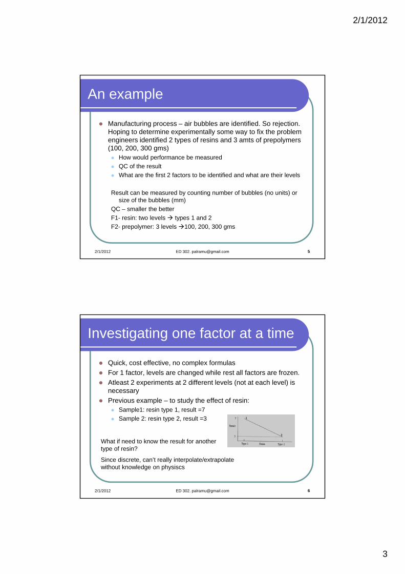
Orthogonal array

Feature of the orthogonal property columns are balanced Each column is balanced within itself (number of times each level

occurs))

Any two column will be balanced ( 4 diff combinations are possible. L4 – only 4 is possible. L8 repeated twice)


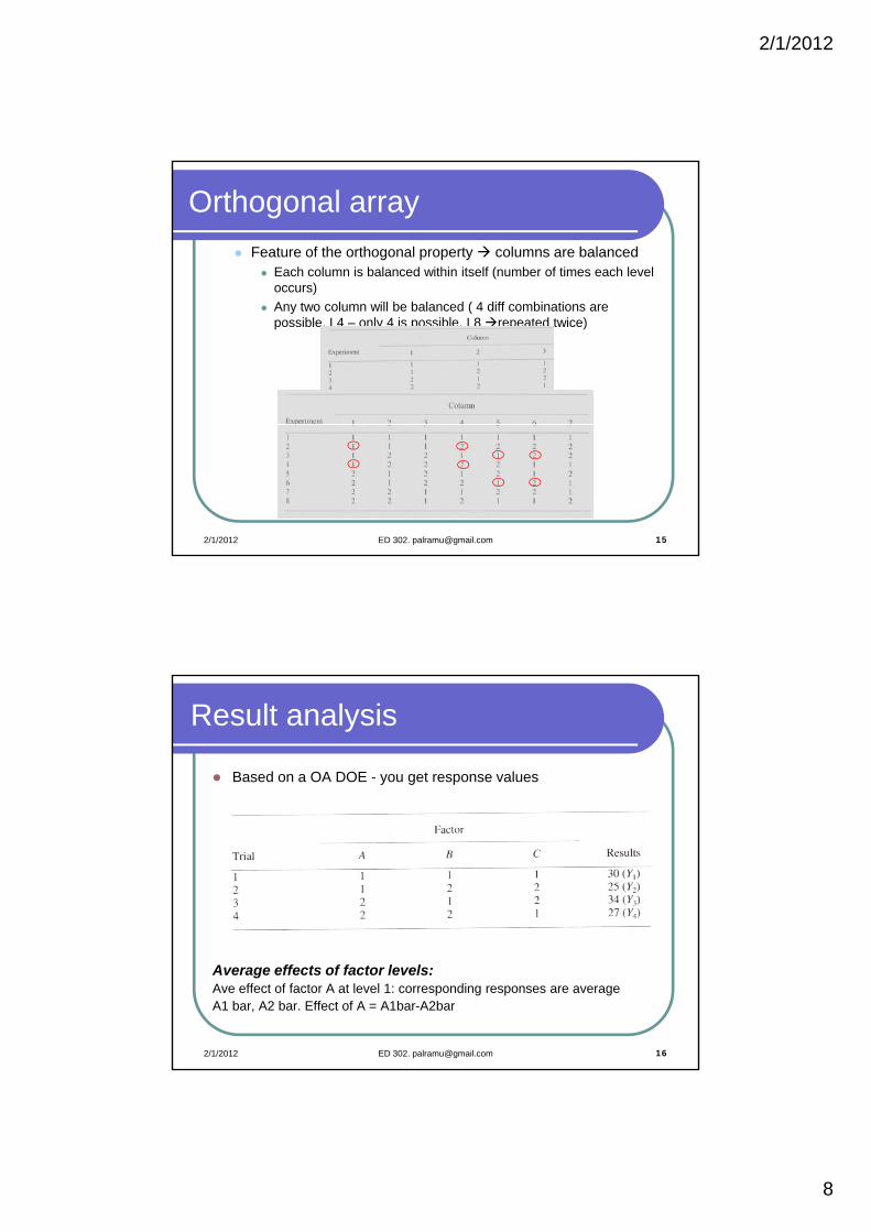
Result analysis

Based on a OA DOE - you get response values


Average effects of factor levels:Ave effect of factor A at level 1: corresponding responses are averageA1 bar, A2 bar. Effect of A = A1bar-A2bar

2/1/2012

9

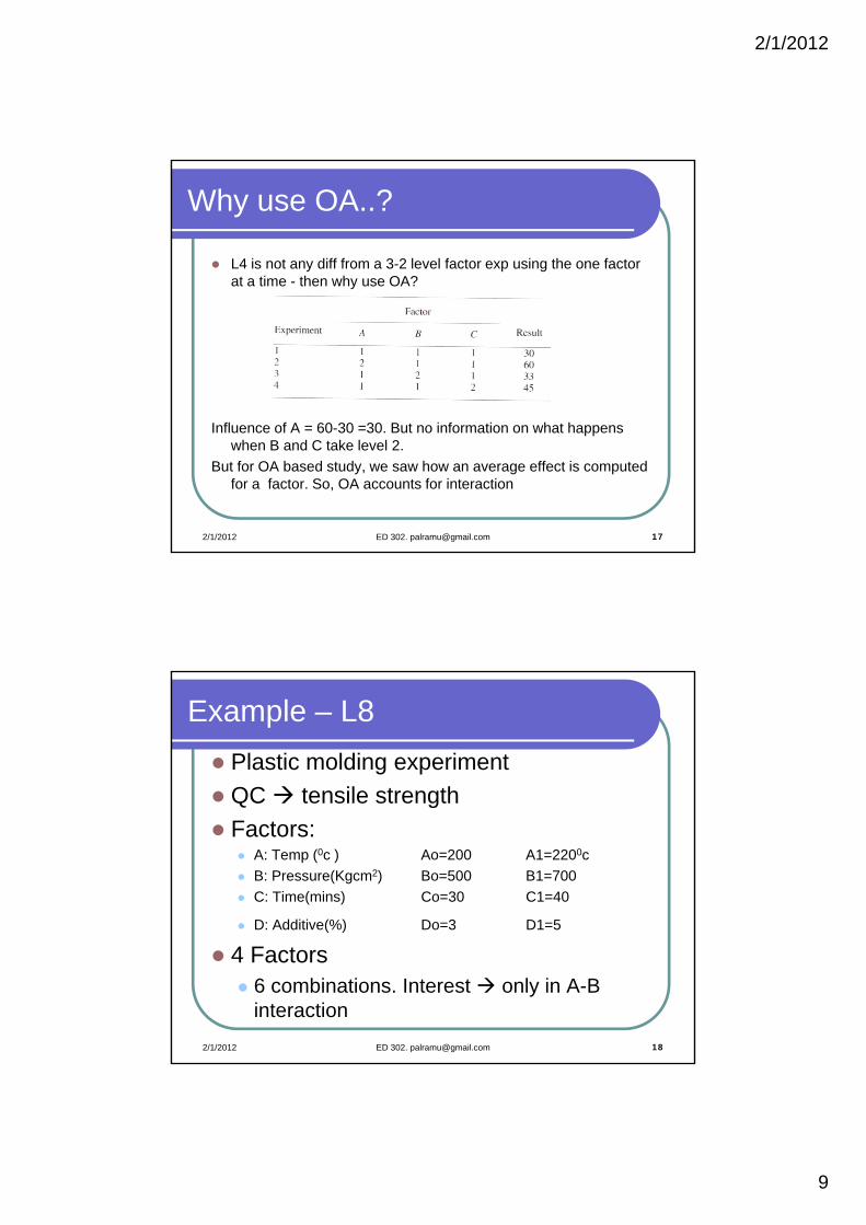
Why use OA..?

L4 is not any diff from a 3-2 level factor exp using the one factor at a time - then why use OA?


Influence of A = 60-30 =30. But no information on what happens when B and C take level 2.

But for OA based study, we saw how an average effect is computed for a factor. So, OA accounts for interaction

Example – L8

Plastic molding experiment

QC tensile strength QC tensile strength

Factors: A: Temp (0c ) Ao=200 A1=2200c

B: Pressure(Kgcm2) Bo=500 B1=700

C: Time(mins) Co=30 C1=40

D: Additive(%) Do=3 D1=5( )

4 Factors 6 combinations. Interest only in A-B

interaction


2/1/2012

10

Factors and Interaction in L8


Anova Table..


2/1/2012

11

LHS designs – 2 factor, 5 realization


When to choose which DOE..?


2/1/2012

12

ANOVA - Analysis of Variance

Once some responses are recorded based on a DOE -how do we go about making conclusions about thehow do we go about making conclusions about the system or the behavior?

We are interested in knowing which level or factor has the major influence on the

final response

Comparing two columns in performance


Consider a 1 factor multiple level problem with multiple experiments

Anova

We are interested in the mean of the observations within each level of our factor. The residuals will tell us about the variation within each level.

We can also average the means of each level to obtain a grand mean. We can then look at the deviation of the mean of each level from the grand mean to understand something about the level effects.

Finally, we can compare the variation within levels to the variation between levels.


This can be easily modelled as:

y(ij) = m + a(i) + e(ij)

The jth data value from level ‘i’. m is the grand mean, a - the level effect and e - the residue

2/1/2012

13

An example of value splittingMachine Level Means

1 2 3 4 5

.1262 .1206 .1246 .1272 .123

Machine

1 2 3 4 5

.125 .118 .123 .126 .118

.127 .122 .125 .128 .129

.125 .120 .125 .126 .127

.126 .124 .124 .127 .120

Residual error (each column deviation)

1 2 3 4 5

-.0012 -.0026 -.0016 -.0012 -.005

.0008 .0014 .0004 .0008 .006

-.0012 -.0006 .0004 -.0012 .004

-.0002 .0034 -.0006 -.0002 -.003

.0018 -.0016 .0014 .0018 -.002


.128 .119 .126 .129 .121 Grand Mean

.12432

LevelEffect (Grand Mean-Level mean)

1 2 3 4 5

.00188 -.00372 .00028 .00288 -.00132

Anova: errors

Variability between the groups and variability within the groups.

Variability between the groups is calculated by first obtaining theVariability between the groups is calculated by first obtaining the sums of squares between groups (SSb), or the sum of the squared differences between each individual group mean from the grand mean.

Variability within the group is calculated by first obtaining the sums of squares within groups (SSw) or the sum of the squared differences between each individual score and that individual’s group mean

SS SS SS


SSt = SSb + SSw

Note that this is a simple linear model that partitions the systematic or explainable deviation (between) and unexplainable (within)

2/1/2012

14

ANOVA Concepts

)xx( 22

Variance is expressed as:

1)x-x (2

N

dfSS2

why N-1..?

Numerator is squared sum and denominator is just DOF


Deviations known to us as variance is referred as mean squares or average of sum of squares while doing ANOVA

b

bb df

SSMS w

wdf

SSMSw

F statistic

F is a statistical distribution used for testing like t distribution in statistics

F (comes from R.A.Fisher) allows you to compare the ratio of variances

Here, we compare:

F= /MS MS


F= /

A F statistic is obtained from the table with n (numerator) and m (denominator) dof . If computed > actual, then reject hypotheses

MSB MSW

2/1/2012

15

ANOVA TABLE

What happens when there are two factors..?

SS-residual – (Res Error)2 =0.00132. DOF – 20

Source Sum of Sq DOF Mean Sq F-value

Factor levels .000137 4 .000034 4.86 > 2.87

residuals .000132 20 .000007

corrected total .000269 24

SS-Level – (Level Effect)2 * number of observations = 0.001137. DOF -4


Reject the hypotheses that the levels are same

Hypotheses testing

Ho: null hypotheses

There is no significant difference among the groups

H1: There is difference atleast with two groups.

There is no accepting a hypotheses but only rejecting or failing to reject

If Fcomputed > Factual - statistically significant

Software give ‘p’ value. Lower the p value, higher is the contribution


2/1/2012

16

Factors that affect significance

The diagrams below show the impact of increasing the numerator of the test statistic. Note that the within group variability (the denominator of th ti ) i th i it ti A d B H th b tthe equation) is the same in situations A and B. However, the betweengroup variability is greater in A than it is in B. This means that the F ratio for A will be larger than for B, and thus is more likely to be significant.


The diagrams below show the impact of decreasing the denominator of the test statistic. Note that the between group variability (the difference b t ) i th i it ti C d D H thbetween group means) is the same in situations C and D. However, the within group variability is greater in D than it is in C. This means that the F ratio for C will be larger than for D, and thus is more likely to be significant.


2/1/2012

17

Full factorial design

Replace 1 by -1 and 2 by 1.Note the main effects and interactions. Higher order interactions are neglected in fractional factorial designs


Fractional design

2K-1 design

Rearranged such that all ABC are 1 (and -1)


g ( ) Effect of ABC is not captured but remaining interaction(s) are captured Coeff of A is equivalent to BC ( B to AC and C to AB) This mix up is called Alias/confounding. Cant differentiate A, BC etc..

2/1/2012

18

How to find alias relationship

Defining relation I = ABC

Premultiply by A

=> A=BC, similarly for other combinations

2k-1 design is 1/2 fraction factorial design and is called the principal fraction

What happens to the second half of the table in the previous slide..?


OA

OA are fractional factorial designs that are orthogonal properties L8 (27 OA)


Linear graphs show interaction relationships

2/1/2012

19

Calculating DOF

Overall mean is 1 always

Each main factor (if levels are na, nb…) = na-1, nb-1

Two factor interaction =(na-1) (nb-1)


Experimental design

Find total number of DOF

Select standard OA using:

Num of runs in OA >=total DOF

Assign factors to appropriate column using linear graph rules


2/1/2012

20


ED302_2012_DOE&Anova

Documents

physiscs2120124one factor

design doe

time discrete factor

multiple factors

continuous factors

design212012 ed

continuous factor ex

resin type