Introductory Applied Econometrics Analysis using Stata November 14 – 18, 2016 Dushanbe, Tajikistan Allen Park and Jarilkasin Ilyasov

Welcome message from author
This document is posted to help you gain knowledge. Please leave a comment to let me know what you think about it! Share it to your friends and learn new things together.
Transcript

Introductory Applied Econometrics
Analysis using Stata
November 14 – 18, 2016
Dushanbe, Tajikistan
Allen Park and Jarilkasin Ilyasov

Linear Regression with One Regressor
Outline
• 1. The population linear regression model
• 2. The ordinary least squares (OLS) estimator and the sample regression line
• 3. Measures of fit of the sample regression
• 4. The least squares assumptions
• 5. The sampling distribution of the OLS estimator
Based on Chapter 4. Stock and Watson. “Introduction to Econometrics” 3rd Edition.

Linear Regression with One Regressor
The population regression line:
• Why are and “population” parameters?
• We would like to know the population value of .
• We don’t know , so must estimate it using data.
10
1
1

Linear Regression with One Regressor
The Population Linear Regression Model
• We have n observations, (Xi, Yi), i = 1,.., n.
• Xi is the independent variable or regressor
• Yi is the dependent variable
• = intercept (the value of population when X=0)
• = slope (change in Y associated with a unit change in X)
• = the regression error (all of the factors )
• The regression error consists of omitted factors. In general, these omitted factors are other factors that influence Y, other than the variable X. The regression error also includes error in the measurement of Y.
0
1u1

Linear Regression with One Regressor
The population regression model in a picture: Observations on Y and
X (n = 7); the population regression line; and the regression error (the “error term”):

Linear Regression with One Regressor
Estimating the coefficient

Linear Regression with One Regressor
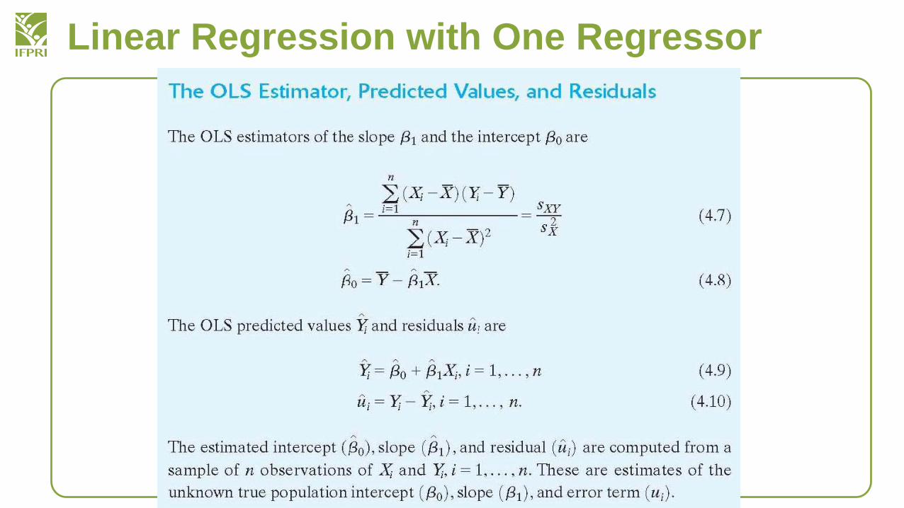
Mechanics of OLS

Linear Regression with One Regressor
The OLS estimator solves:
• The OLS estimator minimizes the average squared difference between the actual values of Yi and the prediction (“predicted value”) based on the estimated line.
• This minimization problem can be solved using calculus (App. 4.2).
Linear Regression with One Regressor

Linear Regression with One Regressor

Linear Regression with One Regressor
Interpretation of the estimated slope and intercept
TestScore = 698.9 – 2.28*STR
• Districts with one more student per teacher on average have test scores that are 2.28 points lower.
• The intercept (taken literally) means that, according to this estimated line, districts with zero students per teacher would have a (predicted) test score of 698.9. But this interpretation of the intercept makes no sense – it extrapolates the line outside the range of the data – here, the intercept is not economically meaningful.
Linear Regression with One Regressor
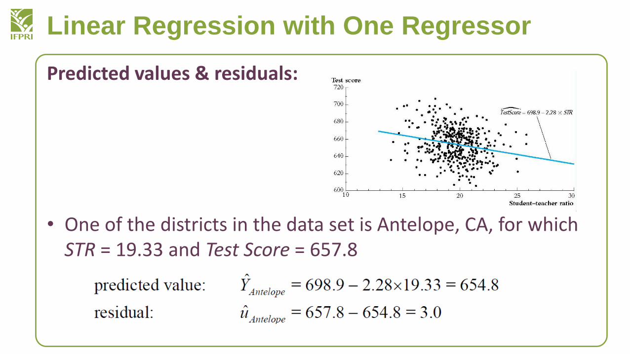
Predicted values & residuals:
• One of the districts in the data set is Antelope, CA, for which STR = 19.33 and Test Score = 657.8

Linear Regression with One Regressor
OLS regression: STATA output
(We’ll discuss the rest of this output later.)

Linear Regression with One Regressor
Measures of Fit
• Two regression statistics provide complementary measures of how well the regression line “fits” or explains the data:
• The regression R2 measures the fraction of the variance of Y that is explained by X; it is unitless and ranges between zero (no fit) and one (perfect fit)
• The standard error of the regression (SER) measures the magnitude of a typical regression residual in the units of Y.
Linear Regression with One Regressor
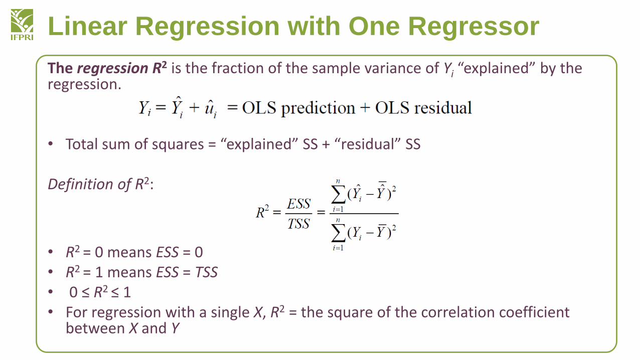
The regression R2 is the fraction of the sample variance of Yi “explained” by the regression.
• Total sum of squares = “explained” SS + “residual” SS
Definition of R2:
• R2 = 0 means ESS = 0• R2 = 1 means ESS = TSS• 0 ≤ R2 ≤ 1• For regression with a single X, R2 = the square of the correlation coefficient
between X and Y
Linear Regression with One Regressor
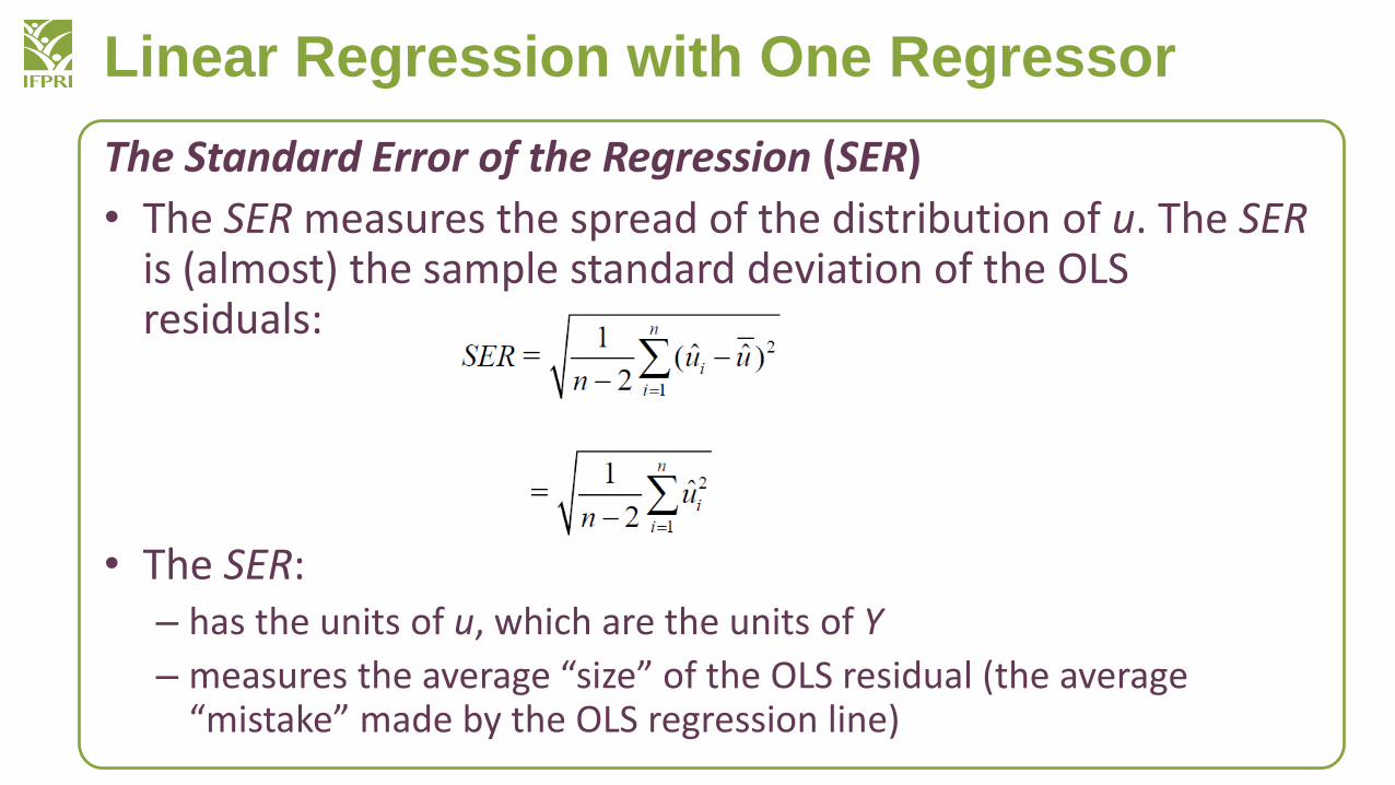
The Standard Error of the Regression (SER)
• The SER measures the spread of the distribution of u. The SER is (almost) the sample standard deviation of the OLS residuals:
• The SER:– has the units of u, which are the units of Y
– measures the average “size” of the OLS residual (the average “mistake” made by the OLS regression line)
Linear Regression with One Regressor
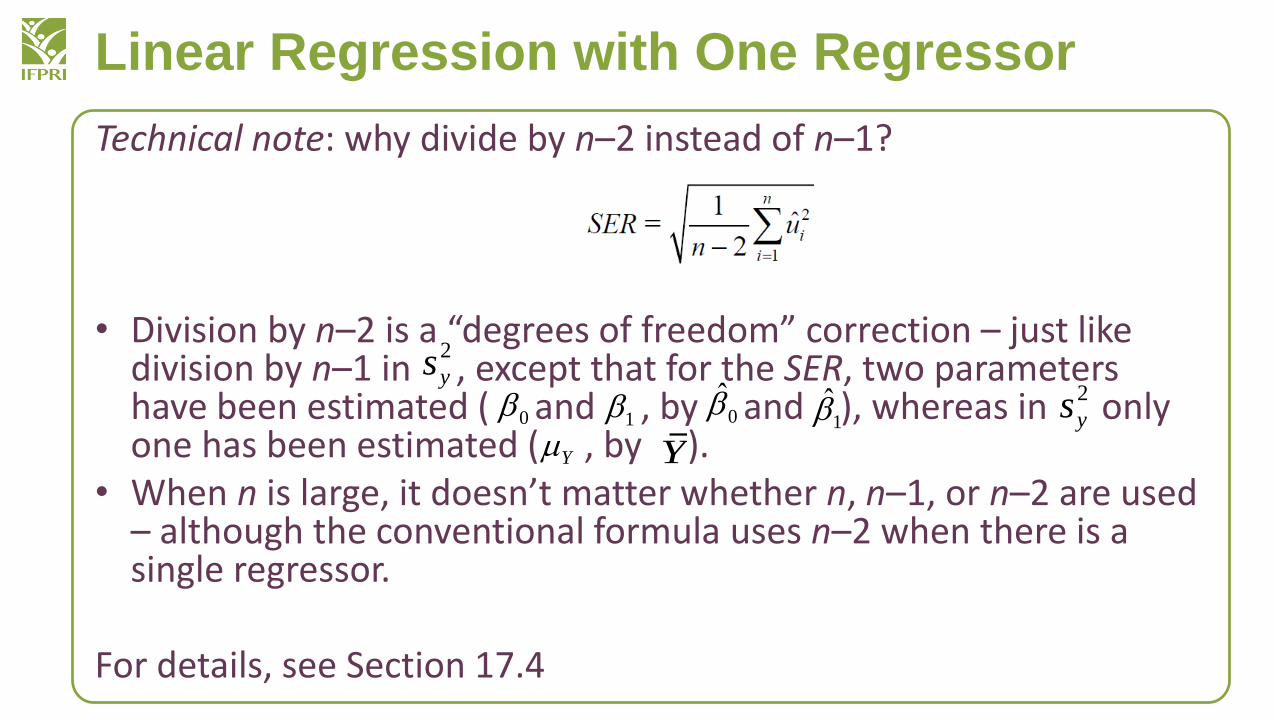
Technical note: why divide by n–2 instead of n–1?
• Division by n–2 is a “degrees of freedom” correction – just like division by n–1 in , except that for the SER, two parameters have been estimated ( and , by and ), whereas in only one has been estimated ( , by ).
• When n is large, it doesn’t matter whether n, n–1, or n–2 are used – although the conventional formula uses n–2 when there is a single regressor.
For details, see Section 17.4
2
ys
0 1 0̂ 1̂2
ys
Y Y

Linear Regression with One Regressor
Example of the R2 and the SER
TestScore = 698.9 – 2.28*STR, R2 = .05, SER = 18.6
• STR explains only a small fraction of the variation in test scores. Does this make sense? Does this mean the STR is unimportant in a policy sense?

Linear Regression with One Regressor
The Least Squares Assumptions
• What, in a precise sense, are the properties of the sampling distribution of the OLS estimator? When will be unbiased? What is its variance?
• To answer these questions, we need to make some assumptions about how Y and X are related to each other, and about how they are collected (the sampling scheme)
• These three assumptions are known as the Least Squares Assumptions.
1

Linear Regression with One Regressor
The Least Squares Assumptions

Linear Regression with One Regressor
Least squares assumption #1: E(u|X = x) = 0 (for any given value of X, the mean of u is zero):

Linear Regression with One Regressor
Least squares assumption #1 (cont.):• A benchmark for thinking about this assumption is to consider an
ideal randomized controlled experiment:– X is randomly assigned to people (students randomly assigned to
different size classes; patients randomly assigned to medical treatments). Randomization is done by computer – using no information about the individual.
– Because X is assigned randomly, all other individual characteristics – the things that make up u – are distributed independently of X, so u and X are independent
– Thus, in an ideal randomized controlled experiment, E(u|X = x) = 0 (that is, LSA #1 holds)
– In actual experiments, or with observational data, we will need to think hard about whether E(u|X = x) = 0 holds.

Linear Regression with One Regressor
Least squares assumption #2: (Xi,Yi), i = 1,…,n are i.i.d.
• This arises automatically if the entity (individual, district) is sampled by simple random sampling:– The entities are selected from the same population, so (Xi, Yi) are
identically distributed for all i = 1,…, n.
– The entities are selected at random, so the values of (X,Y) for different entities are independently distributed.
• The main place we will encounter non-i.i.d. sampling is when data are recorded over time for the same entity (panel data and time series data) – you deal with that complication when we cover panel data.
Linear Regression with One Regressor
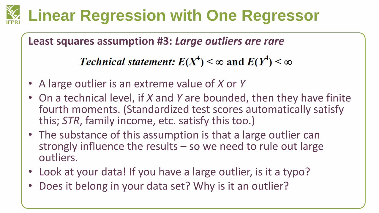
Least squares assumption #3: Large outliers are rare
• A large outlier is an extreme value of X or Y• On a technical level, if X and Y are bounded, then they have finite
fourth moments. (Standardized test scores automatically satisfy this; STR, family income, etc. satisfy this too.)
• The substance of this assumption is that a large outlier can strongly influence the results – so we need to rule out large outliers.
• Look at your data! If you have a large outlier, is it a typo?• Does it belong in your data set? Why is it an outlier?

Linear Regression with One Regressor
OLS can be sensitive to an outlier:
Is the lone point an outlier in X or Y?In practice, outliers are often data glitches (coding or recording problems). Sometimes they are observations that really shouldn’t be in your data set. Plot your data!
Linear Regression with One Regressor
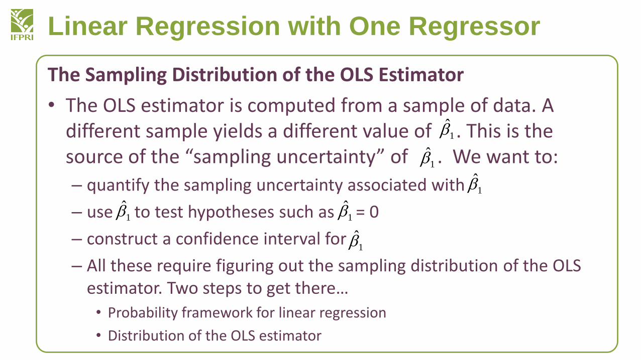
The Sampling Distribution of the OLS Estimator
• The OLS estimator is computed from a sample of data. A different sample yields a different value of . This is the source of the “sampling uncertainty” of . We want to:
– quantify the sampling uncertainty associated with
– use to test hypotheses such as = 0
– construct a confidence interval for
– All these require figuring out the sampling distribution of the OLS estimator. Two steps to get there…
• Probability framework for linear regression
• Distribution of the OLS estimator
1̂
1̂
1̂
1̂ 1̂
1̂

Linear Regression with One Regressor
The probability framework for linear regression is summarized by the three least squares assumptions.
• Population– The group of interest (ex: all possible school districts)
• Random variables: Y, X– Ex: (Test Score, STR)
• Joint distribution of (Y, X). We assume:– The population regression function is linear
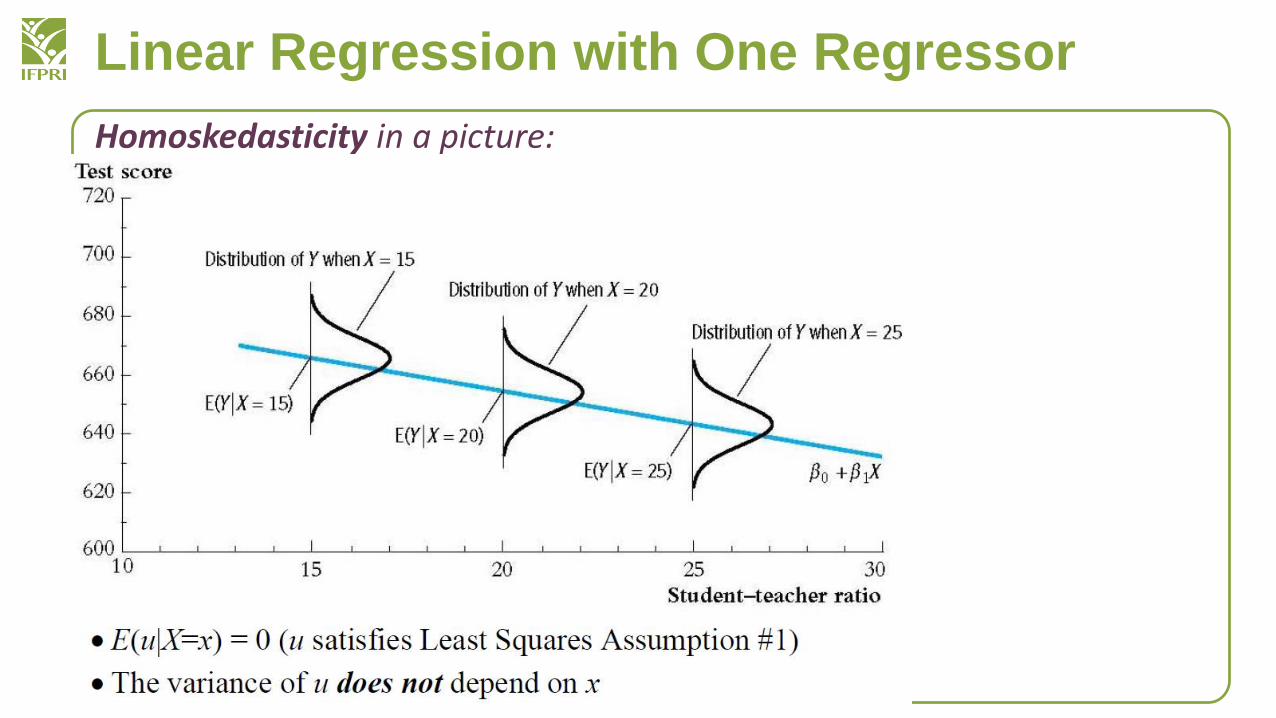
– E(u|X) = 0 (1st Least Squares Assumption)
– X, Y have nonzero finite fourth moments (3rd L.S.A.)
• Data Collection by simple random sampling implies:– {(Xi, Yi)}, i = 1,…, n, are i.i.d. (2nd L.S.A.)

Linear Regression with One Regressor
Summary of Sampling Distribution
• is unbiased: E( )= – just like Y !
• var( )is inversely proportional to n–just like Y!
– The exact sampling distribution is complicated – it depends on the population distribution of (Y, X) – but when n is large we get some simple (and good) approximations.
– The larger the variance of X, the smaller the variance of
1̂ 1̂ 1
1̂
1̂

Linear Regression with One Regressor
• The number of black and blue dots is the same. Using which would you get a more accurate regression line?

Linear Regression with One Regressor
Hypothesis Tests and Confidence Intervals
Outline
• 1. The standard error of
• 2. Hypothesis tests concerning
• 3. Confidence intervals for
• 4. Heteroskedasticity and homoskedasticity
• 5. Efficiency of OLS and the Student t distribution
Based on Chapter 5. Stock and Watson. “Introduction to Econometrics” 3rd Edition.
1
1
1

Linear Regression with One Regressor
A big picture review of where we are going…• We want to learn about the slope of the population regression
line. We have data from a sample, so there is sampling uncertainty. There are five steps towards this goal:
1. State the population object of interest2. Provide an estimator of this population object3. Derive the sampling distribution of the estimator (this requires
certain assumptions). In large samples this sampling distribution will be normal by the CLT.
4. The square root of the estimated variance of the sampling distribution is the standard error (SE) of the estimator
5. Use the SE to construct t-statistics (for hypothesis tests) and confidence intervals.

Linear Regression with One Regressor
• Object of interest: in
• Estimator: the OLS estimator
• The Sampling Distribution of (three assumption of distribution)
1
1
1

Linear Regression with One Regressor
Hypothesis Testing and the Standard Error of
• The objective is to test a hypothesis, like = 0, using data –to reach a tentative conclusion whether the (null) hypothesis is correct or incorrect.
– Null hypothesis can be two-sided:
– Can be one-sided:
1
1

Linear Regression with One Regressor
• General approach: construct t-statistic, and compute p-value (or compare to the N(0,1) critical value)
where is the hypothesized value under the null.
and SE( )= the square root of an estimator of the variance of the sampling distribution of
0,1
1̂
1̂

Linear Regression with One Regressor
Example: Test Scores and STR, California data
Linear Regression with One Regressor
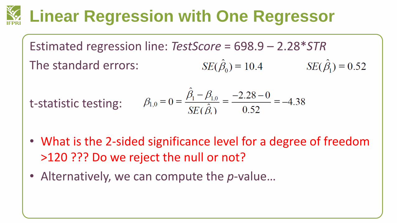
Estimated regression line: TestScore = 698.9 – 2.28*STR
The standard errors:
t-statistic testing:
• What is the 2-sided significance level for a degree of freedom >120 ??? Do we reject the null or not?
• Alternatively, we can compute the p-value…

Linear Regression with One Regressor
The p-value based on the large-n standard normal approximation to the t-statistic is 0.00001 (10-5)

Linear Regression with One Regressor
Confidence Intervals
• Recall that a 95% confidence is, equivalently:
– The set of points that cannot be rejected at the 5% significance level;
– A set-valued function of the data (an interval that is a function of the data) that contains the true parameter value 95% of the time in repeated samples.
Thus:

Linear Regression with One Regressor
The following two statements are equivalent (why?)
• The 95% confidence interval does not include zero;
• The hypothesis = 0 is rejected at the 5% level1

Linear Regression with One Regressor
A concise (and conventional) way to report regressions:
• Put standard errors in parentheses below the estimated coefficients to which they apply.
Standard errors of and0̂ 1̂

Linear Regression with One Regressor
Heteroskedasticity and Homoskedasticity, and Homoskedasticity-Only Standard Errors
What do these two terms mean?
• If var(u|X=x) is constant – that is, if the variance of the conditional distribution of u given X does not depend on X –then u is said to be homoskedastic. Otherwise, u is heteroskedastic.
Linear Regression with One Regressor
Homoskedasticity in a picture:

Linear Regression with One Regressor
Heteroskedasticity in a picture:

Linear Regression with One Regressor
The class size data:
Heteroskedastic or homoskedastic?

Linear Regression with One Regressor
What if the errors are in fact homoskedastic?
• You can prove that OLS has the lowest variance among estimators that are linear in Y… a result called the Gauss-Markov theorem
• We have formulas for standard errors for
– Homoskedasticity-only standard errors
– Heteroskedasticity – robust standard errors
• The main advantage of the homoskedasticity-only standard errors is that the formula is simpler. But the disadvantage is that the formula is only correct if the errors are homoskedastic.
1̂

Linear Regression with One Regressor
Heteroskedasticity-robust standard errors in STATA
• If you use the “, robust” option, STATA computes heteroskedasticity-robust standard errors
• Otherwise, STATA computes homoskedasticity-only standard errors
Related Documents