Stata Guide to Accompany Introductory Econometrics … · 20 Panel data models 135 ... ii. 1 Getting started 1.1 What is Stata? ... Stata users who wish to execute a command that

Stata Guide to Accompany IntroductoryEconometrics for Finance∗

Lisa Schopohl

∗With the author’s permission, this guide draws on material from ‘Introductory Econometrics for Finance’, publishedby Cambridge University Press c© Chris Brooks (2014). The Guide is intended to be used alongside the book, and pagenumbers from the book are given after each section and sub-section heading.

1

Contents

1 Getting started 11.1 What is Stata? . . . . . . . . . . . . . . . . . . . . . . . . . . . . . . . . . . . . . . . . . 11.2 What does Stata look like? . . . . . . . . . . . . . . . . . . . . . . . . . . . . . . . . . . . 11.3 Getting help . . . . . . . . . . . . . . . . . . . . . . . . . . . . . . . . . . . . . . . . . . . 3

2 Data management in Stata 42.1 Variables and data types . . . . . . . . . . . . . . . . . . . . . . . . . . . . . . . . . . . . 42.2 Formats and variable labels . . . . . . . . . . . . . . . . . . . . . . . . . . . . . . . . . . 42.3 Data input and saving . . . . . . . . . . . . . . . . . . . . . . . . . . . . . . . . . . . . . 52.4 Data description . . . . . . . . . . . . . . . . . . . . . . . . . . . . . . . . . . . . . . . . 62.5 Changing data . . . . . . . . . . . . . . . . . . . . . . . . . . . . . . . . . . . . . . . . . . 92.6 Generating new variables . . . . . . . . . . . . . . . . . . . . . . . . . . . . . . . . . . . . 112.7 Plots . . . . . . . . . . . . . . . . . . . . . . . . . . . . . . . . . . . . . . . . . . . . . . . 142.8 Keeping track of your work . . . . . . . . . . . . . . . . . . . . . . . . . . . . . . . . . . 162.9 Saving data and results . . . . . . . . . . . . . . . . . . . . . . . . . . . . . . . . . . . . . 17

3 Simple linear regression - estimation of an optimal hedge ratio 18

4 Hypothesis testing - Example 1: hedging revisited 26

5 Estimation and hypothesis Testing - Example 2: the CAPM 29

6 Sample output for multiple hypothesis tests 34

7 Multiple regression using an APT-style model 357.1 Stepwise regression . . . . . . . . . . . . . . . . . . . . . . . . . . . . . . . . . . . . . . . 38

8 Quantile Regression 40

9 Calculating principal component 45

10 Diagnostic testing 4710.1 Testing for heteroscedasticity . . . . . . . . . . . . . . . . . . . . . . . . . . . . . . . . . 4710.2 Using White’s modified standard error estimates . . . . . . . . . . . . . . . . . . . . . . . 5110.3 The Newey-West procedure for estimating standard errors . . . . . . . . . . . . . . . . . 5210.4 Autocorrelation and dynamic models . . . . . . . . . . . . . . . . . . . . . . . . . . . . . 5310.5 Testing for non-normality . . . . . . . . . . . . . . . . . . . . . . . . . . . . . . . . . . . 5510.6 Dummy variable construction and use . . . . . . . . . . . . . . . . . . . . . . . . . . . . . 5710.7 Multicollinearity . . . . . . . . . . . . . . . . . . . . . . . . . . . . . . . . . . . . . . . . 6110.8 RESET tests . . . . . . . . . . . . . . . . . . . . . . . . . . . . . . . . . . . . . . . . . . 6210.9 Stability tests . . . . . . . . . . . . . . . . . . . . . . . . . . . . . . . . . . . . . . . . . . 63

11 Constructing ARMA models 69

12 Forecasting using ARMA models 77

13 Estimating exponential smoothing models 81

14 Simultaneous equations modelling 83

i

15 VAR estimation 88

16 Testing for unit roots 97

17 Testing for cointegration and modelling cointegrated systems 101

18 Volatility modelling 11518.1 Testing for ‘ARCH effects’ in exchange rate returns . . . . . . . . . . . . . . . . . . . . . 11518.2 Estimating GARCH models . . . . . . . . . . . . . . . . . . . . . . . . . . . . . . . . . . 11618.3 GJR and EGARCH models . . . . . . . . . . . . . . . . . . . . . . . . . . . . . . . . . . 11918.4 GARCH-M estimation . . . . . . . . . . . . . . . . . . . . . . . . . . . . . . . . . . . . . 12218.5 Forecasting from GARCH models . . . . . . . . . . . . . . . . . . . . . . . . . . . . . . . 12418.6 Estimation of multivariate GARCH models . . . . . . . . . . . . . . . . . . . . . . . . . . 126

19 Modelling seasonality in financial data 12919.1 Dummy variables for seasonality . . . . . . . . . . . . . . . . . . . . . . . . . . . . . . . . 12919.2 Estimating Markov switching models . . . . . . . . . . . . . . . . . . . . . . . . . . . . . 130

20 Panel data models 13520.1 Testing for unit roots and cointegration in panels . . . . . . . . . . . . . . . . . . . . . . 141

21 Limited dependent variable models 146

22 Simulation Methods 15622.1 Deriving critical values for a Dickey-Fuller test using simulation . . . . . . . . . . . . . . 15622.2 Pricing Asian options . . . . . . . . . . . . . . . . . . . . . . . . . . . . . . . . . . . . . . 15922.3 VaR estimation using bootstrapping . . . . . . . . . . . . . . . . . . . . . . . . . . . . . . 163

23 The Fama-MacBeth procedure 168

ii

1 Getting started

1.1 What is Stata?

Stata is a statistical package for managing, analysing, and graphing data.1 Stata’s main strengths arehandling and manipulating large data sets, and its ever-growing capabilities for handling panel and time-series regression analysis. Besides its wealth of diagnostic tests and estimation routines, one feature thatmakes Stata a very suitable econometrics software package for both novices and experts of econometricanalyses is that it may be used either as a point-and-click application or as a command-driven package.Stata’s graphical user interface provides an easy interface for those new to Stata and for experiencedStata users who wish to execute a command that they seldom use. The command language providesa fast way to communicate with Stata and to communicate more complex ideas. In this guide we willprimarily be working with the graphical user interface. However, we also provide the correspondingcommand language, where suitable.

This guide is based on Stata 14.0. Please note that if you use an earlier version of Stata the designof the specification windows as well as certain features of the menu structure might differ. As differentstatistical software packages might use different algorithms for some of their estimation techniques theresults generated by Stata might not be comparable to those generated by EViews, in each instance.

A good way of familiarising yourself with Stata is to learn about its main menus and their relation-ships through the examples given in this guide.

This section assumes that readers have a licensed copy of Stata and have successfully loaded it ontoan available computer. There now follows a description of the Stata package, together with instructionsto achieve standard tasks and sample output. Any instructions that must be entered or icons to beclicked are illustrated by bold-faced type. Note that Stata is case-sensitive. Thus, it is importantto enter commands in lower-case and to refer to variables as they were originally defined, i.e. either aslower-case or CAPITAL letters.

1.2 What does Stata look like?

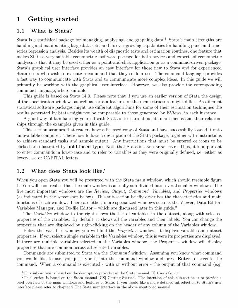
When you open Stata you will be presented with the Stata main window, which should resemble figure1. You will soon realise that the main window is actually sub-divided into several smaller windows. Thefive most important windows are the Review, Output, Command, Variables, and Properties windows(as indicated in the screenshot below). This sub-section briefly describes the characteristics and mainfunctions of each window. There are other, more specialized windows such as the Viewer, Data Editor,Variables Manager, and Do-file Editor – which are discussed later in this guide.2

The Variables window to the right shows the list of variables in the dataset, along with selectedproperties of the variables. By default, it shows all the variables and their labels. You can change theproperties that are displayed by right-clicking on the header of any column of the Variables window.

Below the Variables window you will find the Properties window. It displays variable and datasetproperties. If you select a single variable in the Variables window, this is were its properties are displayed.If there are multiple variables selected in the Variables window, the Properties window will displayproperties that are common across all selected variables.

Commands are submitted to Stata via the Command window. Assuming you know what commandyou would like to use, you just type it into the command window and press Enter to execute thecommand. When a command is executed - with or without error - the output of that command (e.g.

1This sub-section is based on the description provided in the Stata manual [U] User’s Guide.2This section is based on the Stata manual [GS] Getting Started. The intention of this sub-section is to provide a

brief overview of the main windows and features of Stata. If you would like a more detailed introduction to Stata’s userinterface please refer to chapter 2 The Stata user interface in the above mentioned manual.

1

Figure 1: The Stata Main Windows

the table of summary statistics or the estimation output) appears in the Results window. It containsall the commands that you have entered during the Stata session and their textual results . Note thatthe output of a particular test or command shown in the Results window does not differ whether youuse the command language or the point-and-click menu to execute it.

Besides being able to see the output of your commands in the Output window, the command linewill also appear in the Review window at the left-hand-side of the main window. The Review windowshows the history of all commands that have been entered during one session. Note that it displayssuccessfully executed commands in black and unsuccessful commands – along with their error codes –in red. You may click on any command in the Review window and it will reappear in the Commandwindow, where you can edit and/or resubmit it.

The different windows are interlinked. For instance, by double-clicking on a variable in the Variableswindow you can send it to the Command window or you can adjust or re-run certain commands youhave previously executed using the Review window.

There are two ways by which you can tell Stata what you would like it to do: you can directly typein the command into the Command window or you can use the click-and-point menu. Access to theclick-and-point menu can be found at the top left of the Stata main window. You will find that the menuis divided into several sub-categories based on the features they comprise: File, Edit, Data, Graphics,Statistics, User, Window, and Help.

The File menu icon comprises features to open, import, export, print or save your data. Under theData icon you can find commands to explore and manage your data as well as functions to create orchange variables or single observations, to sort data or to merge datasets. The Graphics icon is relativelyself-explanatory as it covers all features related to creating and formatting graphics in Stata. Under theStatistics icon, you can find all the commands and functions to create customised summary statisticsand to run estimations. You can also find postestimation options and commands to run diagnostic(misspecification) tests. Another useful icon is the Help icon under which you can get access to theStata pdf manual as well as other help and search features.

When accessing certain features through the Stata menu (usually) a new dialogue window appearswhere you are asked to specify the task you would like Stata to perform.

Below the menu icons we find the Toolbar. The Toolbar contains buttons that provide quick accessto Stata’s more commonly used features. If you forget what a button does, hold the mouse pointer over

2

the button for a moment, and a tool-tip will appear with a description of that button. In the following,we will focus on those toolbar buttons of particular interest to us.

The Log button begins a new log or closes, suspends, or resumes the current log. Logs are used todocument the results of your session – more on this issue in sub-section 2.8 – Keeping track of yourwork.

The Do-file Editor opens a new do-file or re-opens a previously stored do-file. Do-files are mainlyused for programming in Stata but can also be handy when you want to store a set of commands inorder to allow you to replicate certain analyses at a later point in time. We will discuss in more detailabout the use of do-files and programming Stata in later sections.

There are two icons to open the Data Editor. The Data Editor gives a spreadsheet-like view of thedata. The icon resembling a spreadsheet with a loop opens the Data Editor in the Browse-mode whilethe spreadsheet-like icon with the pen opens the editor in the Edit-mode. The former only allows youto inspect the data. In the edit mode, however, you can make changes to the data, e.g. overwritingcertain data points or dropping observations.

Finally, there are two icons at the very right of the toolbar: a green downward-facing arrow and ared sign with a cross. The former is the Clear–more–Condition icon which tells Stata to continue whenit has paused in the middle of a long output. The latter is the Break icon and pressing it while Stataexecutes a command stops the current task.

1.3 Getting help

There are several different ways to get help when using Stata.3 Firstly, Stata has a very detailed setof manuals which provide several tutorials to explore some of the software’s functionalities. Especiallywhen getting started using Stata, it might be useful to follow some of the examples provided in theStata pdf manuals. These manuals come with the package but can also be direclty accessed via theStata software by clicking on the ‘Help’ icon in the icon menu. There are separate manuals for differentsubtopics, e.g. for graphics, data management, panel data etc. There is also a manual called [GS]Getting started which covers some of the features briefly described in this introduction in more detail.

Sometimes you might need help regarding a particular Stata function or command. For every com-mand, Stata’s in-built support can be called by typing ‘help’ followed by the command in question inthe Command window or via the Help menu icon. The information you will receive is an abbreviatedversion of the Stata pdf manual entry.

For a more comprehensive search or if you do not know what command to use type in ‘search’or ‘findit’ followed by specific keywords. Stata then also provides links to external (web) sources oruser-written commands regarding your particular enquiry.

Besides the help features that come with the Stata package, there is a variety of external resources.For instance, the online Stata Forum is a great source if you have questions regarding specific functional-ities or do not know how to implement particular statistical tests in Stata. Browsing of questions and an-swers by the Stata community is available without registration; if you would like to post questions and orprovide answers to a posted question you need to register to the forum first (http://www.statalist.org/).Another great resource is the Stata homepage. There you can find several video tutorials on a varietyof topics

(http://www.stata.com/links/video-tutorials/ ).Several academics also publish their Stata codes on their institution’s website and several U.S.

institutions provide Stata tutorials that can be accessed via their homepage(e.g. http://www.ats.ucla.edu/stat/stata/ ).

3For a very good overview of Stata’s help features and useful resources please refer to the manual entries ‘4 Gettinghelp’ in the [GS] manual and ‘3 Resources for learning and using Stata’ in the [U] manual.

3

2 Data management in Stata

2.1 Variables and data types

It is useful to learn a bit about the different data types and variable types used in Stata as several Statacommands distinguish between the type of data that you are dealing with and several commands requirethe data to be stored as a certain data type.

Numeric or String Data

We can broadly distinguish between two data types: numeric and string. Numeric is for storing numbers;string resembles a text variable. Variables stored as numeric can be used for computation and inestimations. Stata has different numeric formats or storage types which vary according to the numberof integers they can capture. The more integers a format type can capture the greater its precision, butalso the greater the storage space needed. Stata’s default numeric option is float which stores data as areal number with up to 8 digits. This is sufficiently accurate for most work. Stata also has the followingnumeric storage types available: byte (integer e.g. for dummy variables), int (integer e.g. for yearvariables), long (integer e.g. for population data), and double (real number with 16 digits of accuracy).

Any variable can be designated as a string variable, even numbers. However, in the latter case Statawould not recognise the data as numbers anymore but would treat them as any other text input. Nocomputation or estimations can be performed on string variables. String variables can contain up to 244characters. String values have to be put in quotation marks when being referred to in Stata commands.

To preserve space only store variables with the minimum storage requirements.4

Continuous, categorical and indicator variables

Stata has very convenient functions that facilitate the work and estimation with categorical and indicatorvariables but also other convenient data manipulations such as lags and leads of variables.5

Missing values

Stata marks missing values in series by a dot. Missing numeric observations are denoted by a single dot(.), while missing string observations are referred to either by blank double quotes (“ ”) or dot doublequotes (“.”). Stata can define multiple different missing values, such as .a, .b, .c etc. This might beuseful if you would like to distinguish between the reasons why a data point is missing, such as the datapoint was missing in the original dataset or the data point has been manually removed from the dataset. The largest 27 numbers of each numeric format are preserved for missing values. This is importantto keep in mind when applying constraints in Stata. For example, typing the command ‘describe ageif age>= 27’ includes observations for which the person’s age is missing, while the command ‘describeage if age>=27 & age!=.’ excludes observations with missing age data.

2.2 Formats and variable labels

Each variable may have its own display format. This does not alter the content or precision of thevariable but only affects how it is displayed. You can change the format of a variable by clicking on

4A very helpful command to check whether data can be stored in a data type that requires less storage space is byusing the ‘compress’ command.

5More on this topic can be found in Stata Manual [U] User’s Guide, 25 Working with categorical data and factorvariables.

4

Data / Variable Manager, by directly changing the format in the Variable Manager window at thebottom right of the Stata main screen or by using the command ‘format’ followed by the new formatspecification and the name of the variable. There are different format types that correspond to ordinarynumeric values as well as specific formats for dates and time.

We can attach labels to variables, an entire dataset or to specific values of the variable (e.g. inthe case of categorical or indicator variables). Labelling a variable might be helpful when you want todocument the content of a certain variable or how it has been constructed. You can attach a label to avariable by clicking in the label dialogue box in the Variable Manager window or by clicking on Data/ Variable Manager. A value label can also be attached to a variable using the Variable Managerwindow.6

2.3 Data input and saving

One of the first steps of every statistical analysis is importing the dataset to be analysed into the softwarepackage. Depending on the format of your data there are different ways of accomplishing this task. Ifyour dataset is already in a Stata format which is indicated by the file suffix ‘.dta’ you can click on File/ Open... and simply select the dataset you would like to work with. Alternatively, you use the ‘use’command followed by the name and location of the dataset, e.g. ‘use ”G:\Stata training\sp500.dta”,clear’. The term ‘clear’ tells Stata to close all workfiles that are currently used in memory.

If your dataset is in Excel format you click on File / Import / Excel spreadsheet (*.xls;*.xlsl)and select the Excel file you would like to import into Stata. A new window appears which provides apreview of the data and in which you can specify certain options as to how you would like the datasetto be imported. If you prefer to use a command to import the data you need to type in the command‘import excel’ into the command window followed by the file name and location as well as potentialimporting options.

Stata can also import text data, data in SAS format and other formats (see File / Import) or youcan directly paste observations into the Data Editor. You save changes to your data using the commandsave or by selecting the File / Save as... option in the menu.

When you read data into Stata, it stores it in the RAM (memory). All changes you make aretemporary and will be lost if you close the file without saving it. It is also important to keep in mindthat Stata has no Undo options so that some changes cannot be undone (e.g. dropping of variables).You can generate a snapshot of the data in your Data Editor or by the command ‘snapshot save’ tobe able to reset data to a previous stage.

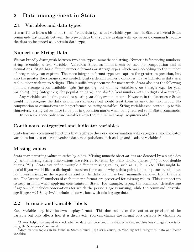
Now let us import a dataset to see how the single steps would be performed. The dataset thatwe want to import into Stata is the excel file UKHP.xls. First, we select File / Import / Excelspreadsheet (*.xls;*.xlsl) and click on the button Browse... . Now we choose the ‘UKHP.xls’ file,click Open and we should find a preview of the data at the bottom of the dialogue window, as shown inFigure 2, left panel. We could further specify the worksheet of the Excel file we would like to import byclicking on the drop-down menu next to the box Worksheet; however, since the ‘UKHP.xls’ file onlyhas one worksheet we leave this box as it is.

The box headed Cell range allows us to specify the cells we would like to import from a specificworksheet. By clicking on the button with the three dots we can define the cell range. In our case wewant the Upper-left cell to be A1 and the lower-right cell to be B270 (see figure 2, right panel). Finally,there are two boxes that can be checked: Import first row as variable names tells Stata that thefirst rows are not to be interpreted as data points but as the names of the variables. Since this is thecase for our ‘UKHP.xls’ we check this box. The second option, Import all data as string tells Stata

6We will not focus on value labels in this guide. The interested reader is advised to refer to the corresponding entriesin the Stata manual to learn more about value labels.

5

Figure 2: Importing excel data into Stata

to store all series as string variables, independent of whether the original series might contain numbers.We want Stata to import our data as numeric values and thus we leave this box unchecked. Once youhave undertaken all these specifications, the dialogue window should resemble figure 2, left panel. Thelast thing we need to do to import the data into Stata is to press OK. If the task has been successfulwe should find the command line import excel followed by the file location and further specificationsin the Output window as well as the Review window. Additionally, there should now be two variablesin the Variables window: Month and AverageHousePrice. Note that Stata automatically attacheda variable label to the two series in the workfile which are identical to the variable names.

You can save the imported dataset as a Stata workfile by clicking on File / Save as... and specifyingthe name of the dataset – in our case ‘ukhp.dta’. Note that we recognise that the dataset is now storedas a Stata workfile by the file-suffix ‘.dta’.

2.4 Data description

Once you have imported your data, you want to get an idea of what the data are like and you want tocheck that all the values have been correctly imported and that all variables are stored in the correctformat.

There are several Stata functions to examine and describe your data. It is often useful to visuallyinspect the data first. This can be done in the Data Editor mode. You can access the Data Editorby clicking on the respective icons in the Stata icon menu as described above. Alternatively, you candirectly use the commands browse or edit.

Additionally, you can let Stata describe the data for you. If you click on Data / Describe datayou will find a variety of options to get information about the content and structure of the dataset.

In order to describe the data structure of the ‘ukhp.dta’ file you can use the describe commandwhich you can find in the Stata menu under Describe data in memory or in a file. It provides thenumber of observations and variables, the size of the dataset as well as variable specifics like storagetype and display format. If we do this for our example session, we are presented with the followingoutput in the Output window.

6

. describe

Contains dataobs: 269vars: 2size: 2,690

storage display valuevariable name type format label variable labelMonth int %tdMon-YY MonthAverageHouseP∼e double %10.0g Average House PriceSorted by:Note: dataset has changed since last saved

.

We see that our dataset contains two variables, one that is stored as ‘int’ and one as ‘double’. Wecan also see the the display format and that the two variables have a variable label but no value labelattached.

The command summarize provides you with summary statistics of the variables. You can find itunder Data / Describe data / Summary statistics. If we click on this option, a new dialoguewindow appears where we can specify what variables we would like to generate summary statistics for(figure 3).

Figure 3: Generating Summary Statistics

If you do not specify any variables, Stata assumes you would like summary statistics for all vari-ables in memory. Again, it provides a variety of options to customise the summary statistics. BesidesStandard display, we can tell Stata to Display additional statistics, or (rather as a programmercommand) to merely calculate the mean without showing any output.7 Using the tab by/if/in allowsus to restrict the data to a sub-sample. The tab Weights provides options to weight the data points inyour sample. However, we want to create simple summary statistics for the two variables in our datasetso we keep all the default specifications and simply press OK. Then the following output should appear

7An application where the latter option will prove useful is presented in later sections of this guide that introduceprogramming in Stata.

7

in our Output window.

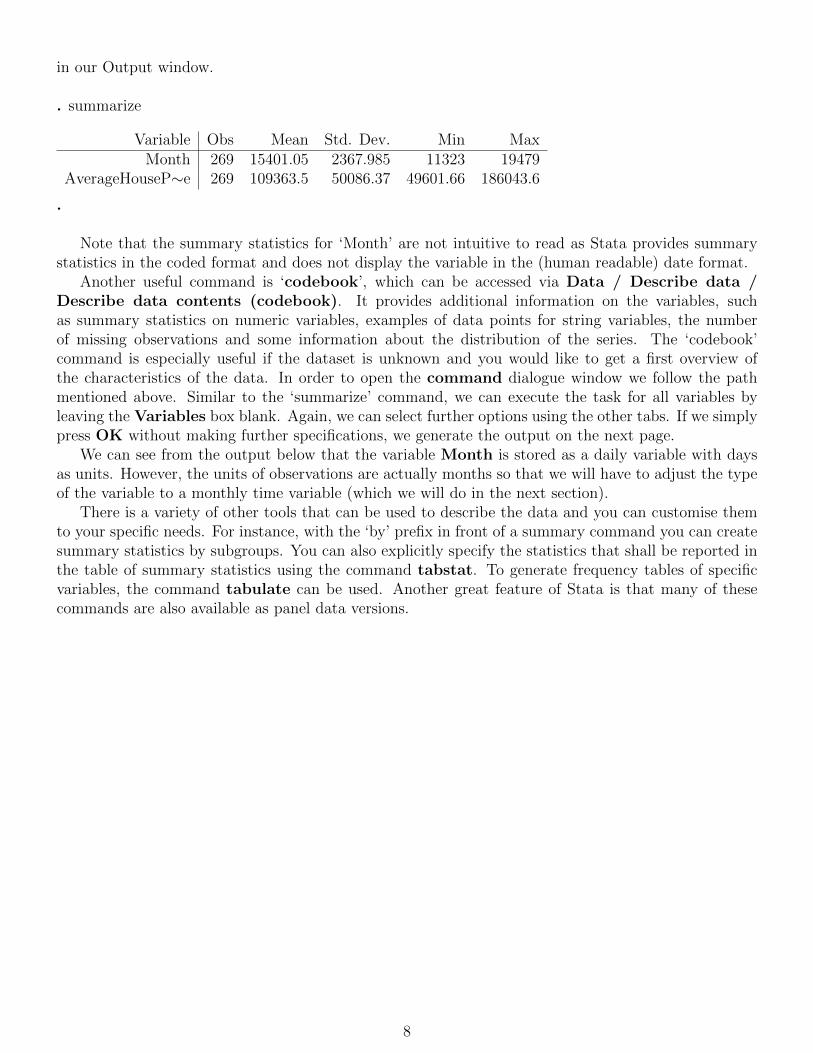
. summarize

Variable Obs Mean Std. Dev. Min MaxMonth 269 15401.05 2367.985 11323 19479

AverageHouseP∼e 269 109363.5 50086.37 49601.66 186043.6

.

Note that the summary statistics for ‘Month’ are not intuitive to read as Stata provides summarystatistics in the coded format and does not display the variable in the (human readable) date format.

Another useful command is ‘codebook’, which can be accessed via Data / Describe data /Describe data contents (codebook). It provides additional information on the variables, suchas summary statistics on numeric variables, examples of data points for string variables, the numberof missing observations and some information about the distribution of the series. The ‘codebook’command is especially useful if the dataset is unknown and you would like to get a first overview ofthe characteristics of the data. In order to open the command dialogue window we follow the pathmentioned above. Similar to the ‘summarize’ command, we can execute the task for all variables byleaving the Variables box blank. Again, we can select further options using the other tabs. If we simplypress OK without making further specifications, we generate the output on the next page.

We can see from the output below that the variable Month is stored as a daily variable with daysas units. However, the units of observations are actually months so that we will have to adjust the typeof the variable to a monthly time variable (which we will do in the next section).

There is a variety of other tools that can be used to describe the data and you can customise themto your specific needs. For instance, with the ‘by’ prefix in front of a summary command you can createsummary statistics by subgroups. You can also explicitly specify the statistics that shall be reported inthe table of summary statistics using the command tabstat. To generate frequency tables of specificvariables, the command tabulate can be used. Another great feature of Stata is that many of thesecommands are also available as panel data versions.

8

. codebook

Month Month

type: numeric daily date (int)

range: [11323,19479] units: 1or equivalently: [01jan1991,01may2013] units: daysunique values: 269 missing .: 0/269

mean: 15401.1 = 02mar2002 (+ 1 hour)std. dev: 2367.99

percentiles: 10% 25% 50% 75% 90%12113 13362 15400 17440 18687

01mar1993 01aug1996 01mar2002 01oct2007 01mar2011

AverageHousePrice Averag House Price

type: numeric (double)

range: [49601.664,186043.58] units: .0001unique values: 269 missing .: 0/269

mean: 109364std. dev: 50086.4

percentiles: 10% 25% 50% 75% 90%51586.3 54541.1 96792.4 162228 168731

.

2.5 Changing data

Often you need to change your data by creating new variables, changing the content of existing dataseries or by adjusting the display format of the data. In the following, we will focus on some of the mostimportant Stata features to manipulate and format the data, though this list is not exhaustive. Thereare several ways you can change data in your dataset. One of the simplest is to rename the variables.For instance, the variable name ‘AverageHousePrice’ is very long and it might be very inconvenient totype such a long name every time you need to refer to it in a Stata task. Thus, we want to change thename of the variable to ‘hp’. To do so, we click on Data / Data utilities and then select Renamegroups of variables. A new dialogue window appears where we can specify exactly how we would liketo rename our variable (figure 4).

As you can see from the list of different renaming options, the dialogue box offers a variety of waysto facilitate renaming a variable, such as changing the case on a variable (from lower-case to upper-case,and vice versa) or by adding a pre- or suffix to a variable. However, we want to simply change the nameof the variable to a predefined name so we keep the default option Rename list of variables. Next,choose the variable we want to rename from the drop-down menu next to the Existing variable names

9

Figure 4: Renaming Variables

box, i.e. AverageHousePrice. Now we simply need to type in the new name in the dialogue box Newvariable names which is hp.8 By clicking OK, Stata performs the command. If we now look at theVariables window we should find that the data series bears the new name. Additionally, we see thatStata shows the command line that corresponds to the ‘rename’ specification we have just performed inthe Output window and the Review window:rename (AverageHousePrice) (hp)

Thus, we could have achieved the same result by typing the above command line into the Commandwindow and pressing Enter.

Stata also allows you to drop specific variables or observations from the dataset, or, alternatively, tospecify the variables and/or observations that should be kept in the dataset, using the drop or keepcommands, respectively. In the Stata menu, these commands can be accessed via Data / Create orchange data / Drop or keep observations. To drop or keep variables, you can also simply right-clickon a variable in the Variables window and select Drop selected variables or Keep only selectedvariables, respectively. As we do not want to remove any variables or observations from our ‘ukhp.dta’dataset, we leave this exercise for future examples.

If you intend to change the content of variables you use the command replace. We can access thiscommand by clicking Data / Create or change data / Change contents of variable. It followsa very similar logic to the command that generates a new variable. As we will explain in detail howto generate new variables in the next section and as we will be using the ‘replace’ command in latersections we will not go into further detail regarding this command.

Other useful commands to change variables are destring and encode. We only provide a briefdescription of the functionalities of each command. The interested reader is advised to learn more aboutthese commands from the Stata pdf manuals. Sometimes Stata does not recognise numeric variables asnumeric and stores them as string instead. destring converts these string data into numeric variables.encode is another command to convert string into numeric variables. However, unlike ‘destring’, theseries that is to be converted into numeric equivalents does not need to be numeric in nature. ‘encode’rather provides a numeric equivalent to a (non-numeric) value, i.e. a coded value.

8Note that using this dialogue window you can rename a group of variables at the same time by selecting all variablesyou would like to rename in the ‘Existing variable names’ box and listing the new names for the variables in the matchingorder in the ‘New variable names’ box.

10

2.6 Generating new variables

One of the most commonly used commands is generate. It creates a new variable having a particularvalue or according to a specific expression. When using the Stata menu we can access it following thepath Data / Create or change data / Create new variable.

Suppose, for example, we have a time series called Z, the latter can be modified in the following waysso as to create variables A, B, C, etc.

A = Z/2 DividingB = Z*2 MultiplicationC = Zˆ2 SquaringD = log(Z) Taking the logarithmsE = exp(Z) Taking the exponentialF = L.Z Lagging the dataG = LOG(Z/L.Z) Creating the log-returnsSometimes you might like to construct a variable containing the mean, the absolute or the standard

deviation of another variable or value. To do so, you will need to use the extended version of the‘generate’ command, the egen function.

Additionally, when creating new variables you might need to employ some logical operators, forexample when adding conditions. Below is a list with the most commonly used logical operators inStata.

== (exactly) equal to!= notequal to> larger than< smaller than>= larger than or equal to<= smaller than or equal to& AND| OR! NOTLet us have a look how to practically generate a new variable. For example, as mentioned earlier,

the variable Month is stored as a daily variable; however, we would like to have a time variable that isstored as a monthly series. Thus, we can use Stata’s ‘generate’ function to create a new monthly timevariable. Using the Stata menu to access the ‘generate’ command, a dialogue box appears where we canspecify the contents of the new variable (figure 5, left panel).

The first thing to be specified is the Variable type. The default is float and for the time being wewill keep the default. Next, we define the name of the new variable. In our case, we could simply usethe lower-case version of month to indicate the monthly series, i.e. Variable name: month.

Next we need to define the Contents of variable by selecting the option Specify a value or anexpression. As stated in the header, the variable content can either be a value, e.g. ‘2’, or it canbe an expression. In our case, we need to specify an expression. If we know the function to convertdaily to monthly data by heart we can simply type it into the respective box. Otherwise, we could usethe ‘Expression builder’ by clicking on Create... next to the box. The ‘Expression builder’ opens andunder Category we select Functions / Date and time (figure 5, right panel). We now see all dateand time-related functions on the left of the window. We look for mofd – i.e. month of day – anddouble click on it. It is then send to the dialogue box at the top of the ‘Expression builder’ window.We type ‘Month’ in between the brackets and press OK. The ‘generate’ dialogue window should nowlook like the left panel of figure 5. We click OK again and we should now find a new variable in theVariable window called ‘month’.

It is useful to perform the codebook command on this variable to see whether we need to make

11

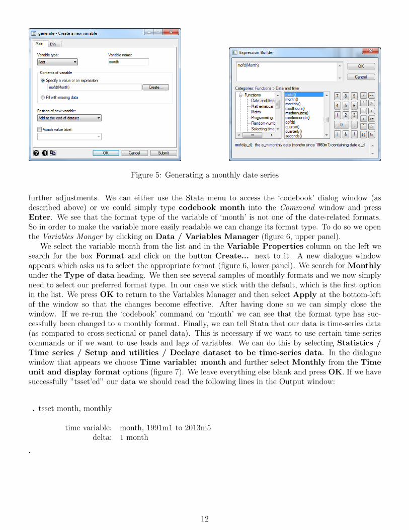
Figure 5: Generating a monthly date series

further adjustments. We can either use the Stata menu to access the ‘codebook’ dialog window (asdescribed above) or we could simply type codebook month into the Command window and pressEnter. We see that the format type of the variable of ‘month’ is not one of the date-related formats.So in order to make the variable more easily readable we can change its format type. To do so we openthe Variables Manger by clicking on Data / Variables Manager (figure 6, upper panel).

We select the variable month from the list and in the Variable Properties column on the left wesearch for the box Format and click on the button Create... next to it. A new dialogue windowappears which asks us to select the appropriate format (figure 6, lower panel). We search for Monthlyunder the Type of data heading. We then see several samples of monthly formats and we now simplyneed to select our preferred format type. In our case we stick with the default, which is the first optionin the list. We press OK to return to the Variables Manager and then select Apply at the bottom-leftof the window so that the changes become effective. After having done so we can simply close thewindow. If we re-run the ‘codebook’ command on ‘month’ we can see that the format type has suc-cessfully been changed to a monthly format. Finally, we can tell Stata that our data is time-series data(as compared to cross-sectional or panel data). This is necessary if we want to use certain time-seriescommands or if we want to use leads and lags of variables. We can do this by selecting Statistics /Time series / Setup and utilities / Declare dataset to be time-series data. In the dialoguewindow that appears we choose Time variable: month and further select Monthly from the Timeunit and display format options (figure 7). We leave everything else blank and press OK. If we havesuccessfully ”tsset’ed” our data we should read the following lines in the Output window:

. tsset month, monthly

time variable: month, 1991m1 to 2013m5delta: 1 month

.

12

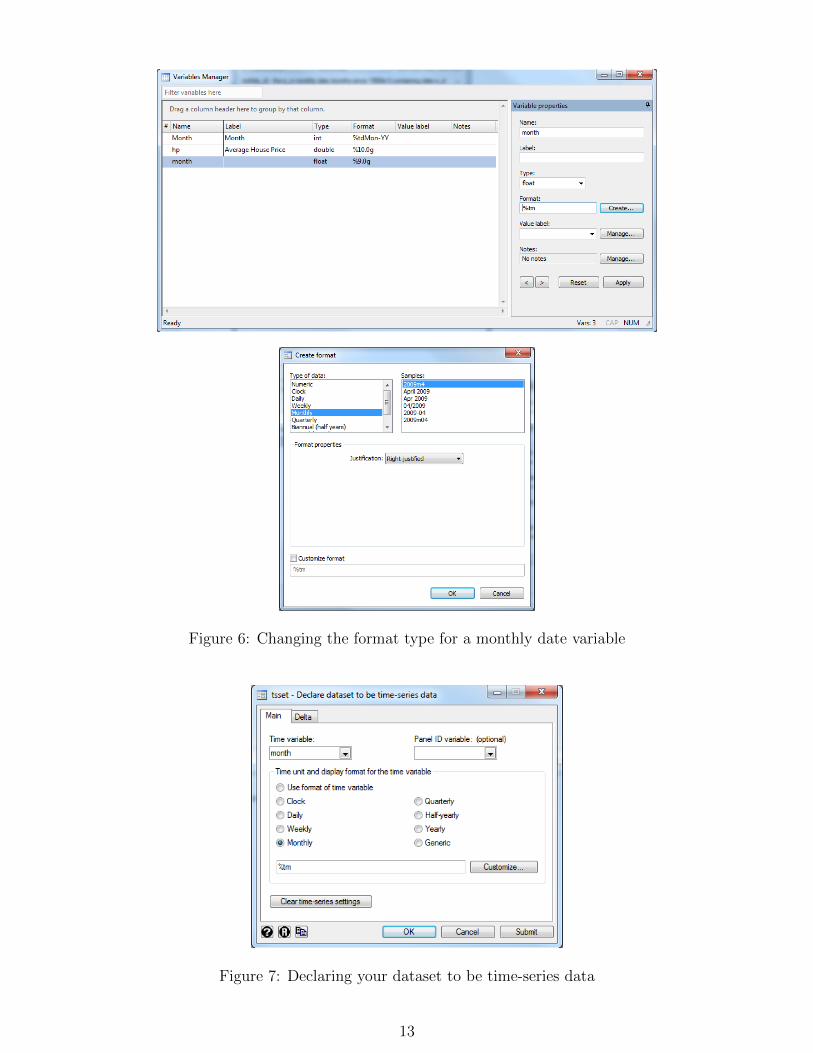
Figure 6: Changing the format type for a monthly date variable

Figure 7: Declaring your dataset to be time-series data

13

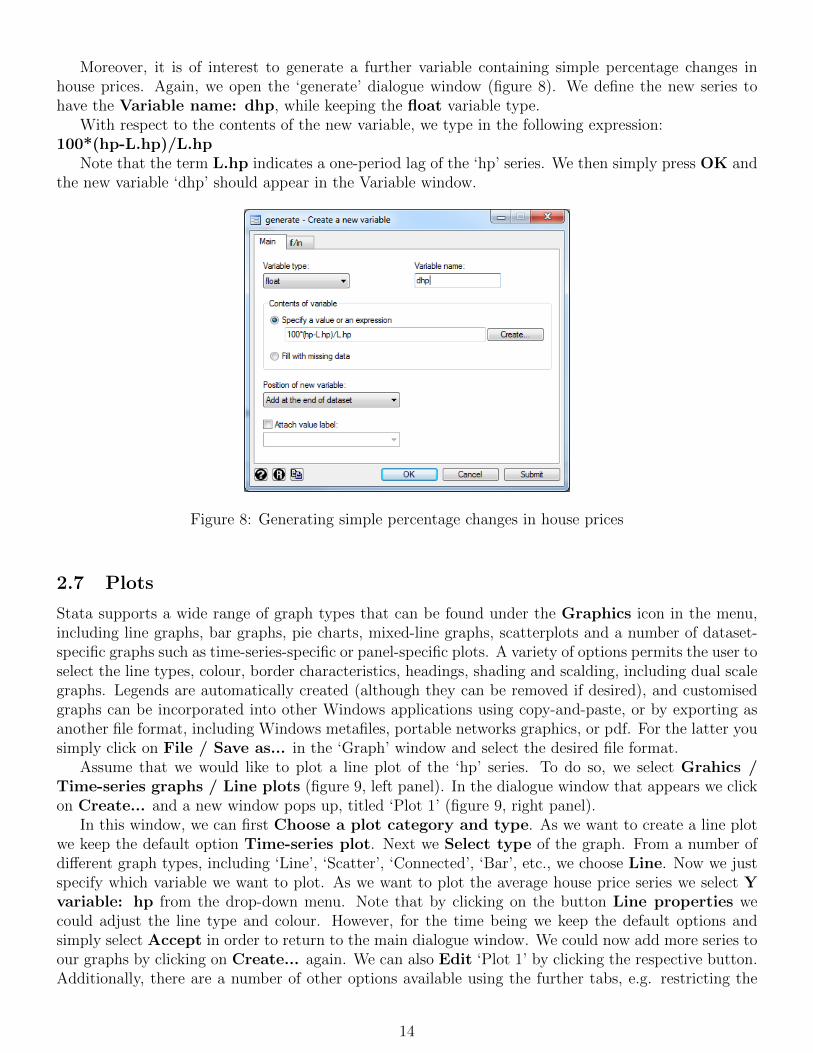
Moreover, it is of interest to generate a further variable containing simple percentage changes inhouse prices. Again, we open the ‘generate’ dialogue window (figure 8). We define the new series tohave the Variable name: dhp, while keeping the float variable type.

With respect to the contents of the new variable, we type in the following expression:100*(hp-L.hp)/L.hp

Note that the term L.hp indicates a one-period lag of the ‘hp’ series. We then simply press OK andthe new variable ‘dhp’ should appear in the Variable window.

Figure 8: Generating simple percentage changes in house prices

2.7 Plots

Stata supports a wide range of graph types that can be found under the Graphics icon in the menu,including line graphs, bar graphs, pie charts, mixed-line graphs, scatterplots and a number of dataset-specific graphs such as time-series-specific or panel-specific plots. A variety of options permits the user toselect the line types, colour, border characteristics, headings, shading and scalding, including dual scalegraphs. Legends are automatically created (although they can be removed if desired), and customisedgraphs can be incorporated into other Windows applications using copy-and-paste, or by exporting asanother file format, including Windows metafiles, portable networks graphics, or pdf. For the latter yousimply click on File / Save as... in the ‘Graph’ window and select the desired file format.

Assume that we would like to plot a line plot of the ‘hp’ series. To do so, we select Grahics /Time-series graphs / Line plots (figure 9, left panel). In the dialogue window that appears we clickon Create... and a new window pops up, titled ‘Plot 1’ (figure 9, right panel).

In this window, we can first Choose a plot category and type. As we want to create a line plotwe keep the default option Time-series plot. Next we Select type of the graph. From a number ofdifferent graph types, including ‘Line’, ‘Scatter’, ‘Connected’, ‘Bar’, etc., we choose Line. Now we justspecify which variable we want to plot. As we want to plot the average house price series we select Yvariable: hp from the drop-down menu. Note that by clicking on the button Line properties wecould adjust the line type and colour. However, for the time being we keep the default options andsimply select Accept in order to return to the main dialogue window. We could now add more series toour graphs by clicking on Create... again. We can also Edit ‘Plot 1’ by clicking the respective button.Additionally, there are a number of other options available using the further tabs, e.g. restricting the

14

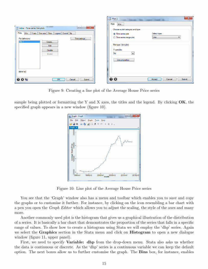
Figure 9: Creating a line plot of the Average House Price series

sample being plotted or formatting the Y and X axes, the titles and the legend. By clicking OK, thespecified graph appears in a new window (figure 10).

Figure 10: Line plot of the Average House Price series

You see that the ‘Graph’ window also has a menu and toolbar which enables you to save and copythe graphs or to customise it further. For instance, by clicking on the icon resembling a bar chart witha pen you open the Graph Editor which allows you to adjust the scaling, the style of the axes and manymore.

Another commonly used plot is the histogram that gives us a graphical illustration of the distributionof a series. It is basically a bar chart that demonstrates the proportion of the series that falls in a specificrange of values. To show how to create a histogram using Stata we will employ the ‘dhp’ series. Againwe select the Graphics section in the Stata menu and click on Histogram to open a new dialoguewindow (figure 11, upper panel).

First, we need to specify Variable: dhp from the drop-down menu. Stata also asks us whetherthe data is continuous or discrete. As the ‘dhp’ series is a continuous variable we can keep the defaultoption. The next boxes allow us to further customise the graph. The Bins box, for instance, enables

15

Figure 11: Creating a histogram

us to choose the number of bins or the bin width. Using the Y axis box we can also select whetherthe histogram shall be expressed in terms of the density, the faction, frequency or percentage of thedistribution. Additionally, there are a series of other adjustment options available when using thefurther tabs. We simply click OK and the histogram of the ‘dhp’ series should resemble figure 11, lowerpanel. Feel free to change some of the specifications and see their effect on the plot.

2.8 Keeping track of your work

In order to be able to reproduce your work and remember what you have done after some time, youcan record both the results and the list of commands. To record the outputs that appear in the Resultswindow, use Log files. Open a new log file by clicking on the respective icon in the Stata toolbar.Log files can be printed or saved in other file formats. When returning to a Stata session, you can alsoappend a log file saved during a previous session.

Do-files can be used to record the set of commands that you have used during a session. Put simply,a do-file is a single file that lists a whole set of commands. This enables you to execute all commandsin one go or only a selection of the commands. By saving the do-files you are able to easily replicate

16

analyses done in previous Stata sessions. Do-files can be written in any text editor, such as Word orNotepad. It is good practice to keep extensive notes within your do-file so that when you look back overit you know what you were trying to achieve with each command or set of commands. We will be usingdo-files in later sections of this guide so will leave a more detailed description of do-files and the ‘Do-fileEditor’ until then.

2.9 Saving data and results

Data generated in Stata can be exported to other Windows applications, e.g. Microsoft Excel, or toa data format used by other statistical software packages, e.g. SAS. To export data, click on File /Export and then choose the file type required. In the ‘export’ dialogue window you can then specifythe variables to export or you can restrict the sample to export. You also need to specify a file nameand location for the new file.

You can export single outputs by highlighting them in the Results window, then right-clicking onthe highlighted section and choosing the ‘Copy’ option required. For example, you can copy as a table(and paste the results into Excel) or you can copy as a picture.

Additionally, there are several other commands that can be used to save estimation results or togenerate formatted tables of results. Some useful commands are, for example, ‘estimates save’ or theuser-written command ‘outreg2’.9 We leave it to the interested reader to learn more about Stata’soptions to export estimation results in the Stata manual.

9The latter is a user-written ado-file that needs to be installed before you can use it. This can be easily done by typing‘findit outreg2’ into your command window and clicking on the link for outreg2. Once you have installed it, you can useit as if it was a built-in Stata function. It also has its own help description that you can access via the command ‘helpoutreg2’.

17

3 Simple linear regression - estimation of an optimal hedge

ratio

Reading: Brooks (2014, section 3.5)This section shows how to run a bivariate regression using Stata. In our example an investor wishes

to hedge a long position in the S&P500 (or its constituent stocks) using a short position in futurescontracts. The investor is interested in the optimal hedge ratio, i.e. the number of units of the futuresasset to sell per unit of the spot assets held.10

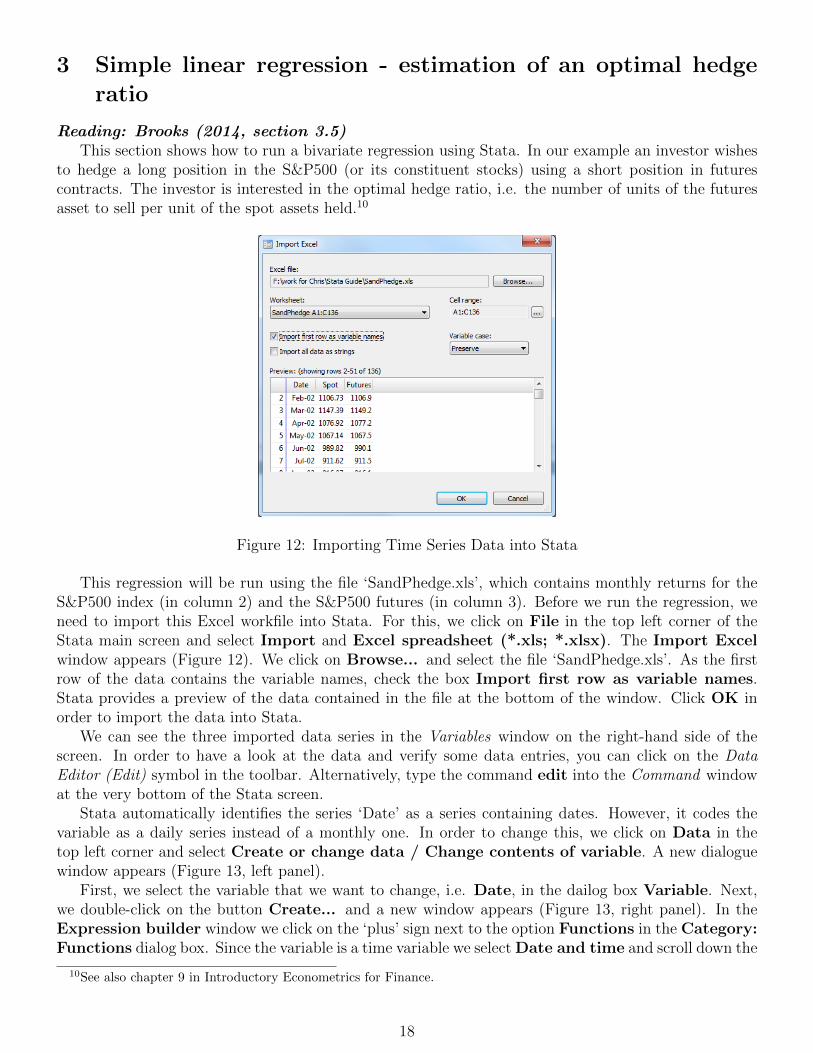
Figure 12: Importing Time Series Data into Stata

This regression will be run using the file ‘SandPhedge.xls’, which contains monthly returns for theS&P500 index (in column 2) and the S&P500 futures (in column 3). Before we run the regression, weneed to import this Excel workfile into Stata. For this, we click on File in the top left corner of theStata main screen and select Import and Excel spreadsheet (*.xls; *.xlsx). The Import Excelwindow appears (Figure 12). We click on Browse... and select the file ‘SandPhedge.xls’. As the firstrow of the data contains the variable names, check the box Import first row as variable names.Stata provides a preview of the data contained in the file at the bottom of the window. Click OK inorder to import the data into Stata.

We can see the three imported data series in the Variables window on the right-hand side of thescreen. In order to have a look at the data and verify some data entries, you can click on the DataEditor (Edit) symbol in the toolbar. Alternatively, type the command edit into the Command windowat the very bottom of the Stata screen.

Stata automatically identifies the series ‘Date’ as a series containing dates. However, it codes thevariable as a daily series instead of a monthly one. In order to change this, we click on Data in thetop left corner and select Create or change data / Change contents of variable. A new dialoguewindow appears (Figure 13, left panel).

First, we select the variable that we want to change, i.e. Date, in the dailog box Variable. Next,we double-click on the button Create... and a new window appears (Figure 13, right panel). In theExpression builder window we click on the ‘plus’ sign next to the option Functions in the Category:Functions dialog box. Since the variable is a time variable we select Date and time and scroll down the

10See also chapter 9 in Introductory Econometrics for Finance.

18

Figure 13: Changing the Unit of Date Variables

options on the right until we find the function mofd().11 We double-click on mofd() and the expressionappears in the dialog box in the top of the window. We type Date in between the parentheses and clickon OK. The expression now appears in the dialog box New contents: (value or expression).12 Byclicking OK Stata will replace the daily variable ‘Date’ with its monthly equivalent.13

In order to change the display format of the changed variable from a daily to a monthly format, weclick Data in the top left menu and select Variable Manager. In the newly appearing window we selectthe variable Date and click the box Create... next to the Format dialogue box on the left (Figure 14,upper panel).

A new window appears (Figure 14, lower panel). We specify the Type of data to be Monthly andclick OK.14 To make these changes effective, we click on Apply at the bottom right of the window.Afterwards, we just close the Variable Manager window. In order to see the effect of these changes,change to the Data Editor by clicking on the respective symbol in toolbar or, alternatively, type in thecommand edit in the Command window.

As we want to perform time series regressions, we need to tell Stata which of the three variables isthe time indicator. To do so, we click on Statistics in the top right menu and select Time Series/ Setup and Utilities / Declare dataset to be time-series data. In the dialogue box we selectthe time variable Date and further specify that the Time unit and display format of the timevariable is Monthly (Figure 15). We can ignore the other options for now.

By clicking OK, the command together with the specifications of the time variable ‘Date’ appearin the Output window. ‘delta: 1 month’ indicates that the time variable is monthly data and that thedifference between a data entry and the consecutive data entry is 1 month.15

We run our analysis based on returns of the S&P500 index instead of price levels; so the next step

11mofd() is an abbreviation for month of date and returns the monthly date of a variable that contains daily dates.12Alternatively, if you know the function to use, you can directly input the expression in the dialogue box New contents:

(value or expression).13The command for this data manipulation appears in the Review window on the left. By clicking on it, it appears in

the Command window at the bottom of the Stata screen. As a (faster) alternative than using the ‘point-or-click’ menuto execute the data manipulation, we could have directly typed the command in the Command window.

14In the dialogue box Samples, we can choose between different ways of displaying the monthly data series. Theseoptions merely represent different display formats and do not change the characteristics of the underlying series. Thechoice of the display format depends on personal taste so choose the format that is most appealing to you.

15Note that if we had not changed ‘Date’ from a daily data series into a monthly data series the data unit would beindicated as ‘1 day’. This might lead to problems in case we want to execute time operators in further analyses.

19

Figure 14: Variable Manager

is to transform the ‘Spot’ and ‘Futures’ price series into percentage returns. For our analysis we usecontinuously compounded returns, i.e. logarithmic returns, instead of simple returns as it is common inacademic finance research. To generate a new data series of continuously compounded returns, we clickon Data and select Create or change data / Create new variable. A new window appears wherewe can specify the new variable we want to create (Figure 16).

20

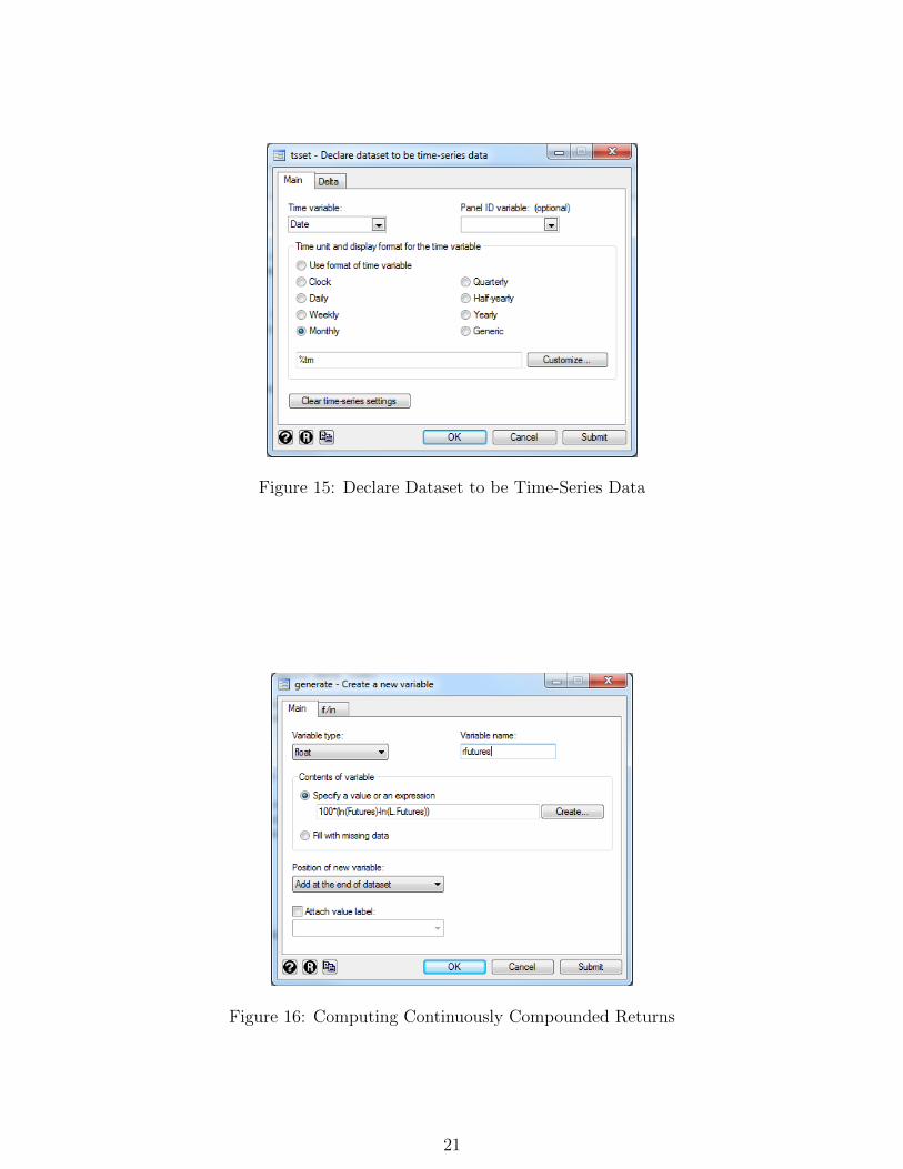
Figure 15: Declare Dataset to be Time-Series Data

Figure 16: Computing Continuously Compounded Returns

21

We keep the default Variable type specification of float which specifies that the newly createdvariable is a data series of real numbers with about 8 digits.16 We name the new variable rfutures inthe Variable name dialogue box. Next, we enter 100*(ln(Futures)-ln(L.Futures)) into the dialogbox that asks to Specify a value or an expression. ‘ln()’ generates the natural logarithm of the dataseries and ‘L.’ represents a time operator indicating a 1-period lagged value of the variable ‘Futures’.17

To generate the new variable, we click on OK.Next, we generate continuously compounded returns for the ‘Spot’ price series. We can either use

the Stata ‘point-or-click’ menu and repeat the steps described above with the ‘Spot’ series; or, as a fasteralternative, we can directly type in the command in the Command window. In the latter case, we typegenerate rspot = 100*(ln(Spot)-ln(L.Spot))and press Enter to execute the command.

Do not forget to save the workfile selecting File and Save as.... Call the workfile ‘hedge.dta’.Continue to re-save the file at regular intervals to ensure that no work is lost.

Before proceeding to estimate the regression, now that we have imported more than one series, wecan examine a number of descriptive statistics together and measures of association between the series.For the summary statistics, we click on Data and Describe data / Summary Statistics. In thedialogue box that appears, we type (or select from the drop-down menu) rspot rfutures and click OK(Figure 17).

Figure 17: Generating Summary Statistics

The following summary statistics appear in the Output window:. summarize rspot rfuturesVariable Obs Mean Std. Dev. Min Max

rspot 134 .2739265 4.591529 -18.38397 10.06554rfutures 134 .2713085 4.548128 -18.80256 10.39119

.

16An accuracy of eight digits is sufficiently accurate for most work. However, if you need a higher accuracy of the data,e.g. as you are working with very small decimal number, you can change the variable type to double which creates avariable with an accuracy of 16 digits.

17In order to use the time operators, the time series operator needs to be set using the tsset command described above.Time series operators are a very useful Stata tool. For more information on time series operators type in help tsvarlistin the Command box and corresponding chapter in the Data documentation.

22

We observe that the two return series are quite similar as based on their mean values, standarddeviations, as well as minimum and maximum values, as one would expect from economic theory.18

Note that the number of observations has reduced from 135 for the levels of the series to 134 whenwe computed the returns (as one observation is ‘lost’ in constructing the t − 1 value of the prices inthe returns formula). If you want to save the summary statistics, you must either highlight the table,left-click, (Copy table) and paste it into an Excel spreadsheet; or you open a log file before undertakingthe analysis which will record all command outputs displayed in the Output window. To start a log, weclick on the Log symbol (which resembles a notepad) in the menu and save it. Remember to close thelog file when you have finished the analyses by clicking on the Log symbol again and selecting Closelog file.

We can now proceed to estimate the regression. We click on Statistics and choose the second optionin the list, Linear models and related and Linear regression. In the dialogue window titled ‘regress- Linear regression’, we first specify the dependent variable (y), rspot (Figure 18).

Figure 18: Estimating OLS Regressions

The independent variable is the rfutures series. Thus, we are trying to explain variations in thespot rates with variations in the futures rates. Stata automatically includes a constant term in the linearregression; therefore you do not specifically include it among the independent variables. If you do notwish to include a constant term in the regression you need to check the box Suppress constant term.The regress command estimates an OLS regression based on the whole sample. You can customise theregression specification, e.g. with respect to the selected sample or the treatment of standard errors, byusing the other tabs. However, for now we stick with the default specification and press OK in orderto run the regression. The regression results will appear in the Output window as follows:

18Stata allows to customise your summary statistics by choosing the type of statistics and their order. For this you canuse the tabstat command. Click on Statistics and Summaries, tables,and tests. Select Other tables and Compacttable of summary statistics. Specify the variables in the ‘Variables’ dialogue box. Next select and specify the numberand type of Statistics to display by checking the box next to the statistic and selecting the statistic of choice fromthe drop-down menu. Once you have finalised your selection, click on OK and the summary statistics will appear in theOutput window.

23

. regress rspot rfutures

Source SS df MS Number of obs = 134F( 1, 132) = 29492.60

Model 2791.43107 1 2791.43107 Prob > F = 0.0000Residual 12.4936054 132 .094648526 R-squared = 0.9955

Adj R-squared = 0.9955Total 2803.92467 133 21.0821404 Root MSE = .30765

rspot Coef. Std. Err. t P>|t| [95% Conf. Interval]rfutures 1.007291 .0058654 171.73 0.000 .9956887 1.018893

cons .0006399 .0266245 0.02 0.981 -.052026 .0533058

.

The parameter estimates for the intercept (α) and slope (β) are 0.00064 and 1.007 respectively.19 Alarge number of other statistics are also presented in the regression output – the purpose and interpre-tation of these will be discussed later.

Now we estimate a regression for the levels of the series rather than the returns (i.e. we run aregression of ‘Spot’ on a constant and ‘Futures’) and examine the parameter estimates. We can eitherfollow the steps described above and specify ‘Spot’ as the dependent variable and ‘Futures’ as theindependent variable; or we can directly type the command into the Command window asregress Spot Futuresand press Enter to run the regression (see below). The intercept estimate (α) in this regression is 5.4943and the slope estimate (β) is 0.9956.

. regress Spot Futures

Source SS df MS Number of obs = 135F( 1, 132) = .

Model 5097856.27 1 5097856.27 Prob > F = 0.0000Residual 2406.03961 133 18.0905234 R-squared = 0.9995

Adj R-squared = 0.9995Total 5100262.31 134 38061.659 Root MSE = 4.2533

Spot Coef. Std. Err. t P>|t| [95% Conf. Interval]Futures .9956317 .0018756 530.85 0.000 .991922 .9993415

cons 5.494297 2.27626 2.41 0.017 .9919421 9.996651

.

Let us now turn to the (economic) interpretation of the parameter estimates from both regressions.The estimated return regression slope parameter measures the optimal hedge ratio as well as the shortrun relationship between the two series. By contrast, the slope parameter in a regression using the rawspot and futures indices (or the log of the spot series and the log of the futures series) can be interpretedas measuring the long run relationship between them. The intercept of the price level regression can beconsidered to approximate the cost of carry. Looking at the actual results, we find that the long-term

19Note that in order to save the regression output you have to Copy table as described above for the summary statisticsor remember to start a log file before undertaking the analysis. There are also other ways to export regression results.For more details on saving results please refer to section 2.9 of this guide.

24

relationship between spot and futures prices is almost 1:1 (as expected).Before exiting Stata, do not forget to click the Save button to save the whole workfile.

25

4 Hypothesis testing - Example 1: hedging revisited

Brooks (2014, section 3.15)Let us now have a closer look at the results table from the returns regressions in the previous section

where we regressed S&P500 spot returns on futures returns in order to estimate the optimal hedge ratiofor a long position in the S&P500. If you do not have the results ready on your Stata main screen,reload the ‘SandPhedge.dta’ file now and re-estimate the returns regression using the steps described inthe previous section (or, alternatively, type in regress rspot rfutures into the Command window andexecute the command). While we have so far mainly focused on the coefficient estimates, i.e. α and βestimates, Stata has also calculated several other statistics which are presented next to the coefficientestimates: standard errors, the t-ratios and the p-values.

The t-ratios are presented in the third column indicated by the ‘t’ in the column heading. They arethe test statistics for a test of the null hypothesis that the true values of the parameter estimates arezero against a two-sided alternative, i.e. they are either larger or smaller than zero. In mathematicalterms, we can express this test with respect to our coefficient estimates as testing H0 : α = 0 versusH1 : α 6= 0 for the constant ‘ cons’ in the second row of numbers and H0 : β = 0 versus H1 : β 6= 0 for‘rfutures’ in the first row. Let us focus on the t-ratio for the α estimate first. We see that with a valueof only 0.02 the t-ratio is very small which indicates that the corresponding null hypothesis H0 : α = 0is likely not to be rejected. Turning to the slope estimate for ‘rfutures’, the t-ratio is high with 171.73suggesting that H0 : β = 0 is to be rejected against the alternative hypothesis of H1 : β 6= 0. Thep-values presented in the fourth column, ‘P>|t|’, confirm our expectations: the p-value for the constantis considerably larger than 0.1 meaning that the corresponding t-statistic is not even significant at a10% level; in comparison, the p-value for the slope coefficient is zero to, at least, three decimal points.Thus, the null hypothesis for the slope coefficient is rejected at the 1% level.

While Stata automatically computes and reports the test statistics for the null hypothesis that thecoefficient estimates are zero, we can also test other hypotheses about the values of these coefficientestimates. Suppose that we want to test the null hypothesis that H0 : β = 1. We can, of course,calculate the test statistics for this hypothesis test by hand; however, it is easier if we let Stata do thiswork. For this we use the Stata command ‘test’. ‘test’ performs Wald tests of simple and compositelinear hypotheses about the parameters of the most recently fit model.20 To access the Wald test, weclick on Statistics and select Postestimation (second option from the bottom). The new windowtitled ‘Postestimation Selector’ appears (figure 19). We select Tests, contrasts, and comparisons ofparameter estimates and then chose the option Linear tests of parameter estimates.

The ‘test’ specification window should appear (figure 20, upper panel). We click on Create next toSpecification 1 and a new window, titled ‘Specification 1’ appears (figure 20, bottom panel). In thebox Test type we choose the second option Linear expressions are equal and we select Coefficient:rfutures. This is because we want to test a linear hypothesis that the coefficient estimate for ‘rfutures’is equal to 1. Note that the first specification Coefficients are 0 is equal to the test statistics for thenull hypothesis H0 : β = 0 versus H1 : β 6= 0 for the case of ‘rfutures’ that we discussed above and thatis automatically reported in the regression output.21 Next, we specify the linear expression we wouldlike to test in the dialog box Llinear expression. In our case we type in rfutures=1. To generatethe test statistic, we press OK and again OK. The Stata output on the following page after the figuresshould appear in the Output window.

20Thus, if you want to do a t-test based on the coefficient estimates of the return regression make sure that the returnregression is the last regression you estimated (and not the regression on price levels).

21For more information on the ‘test’ command and the specific tests it can perform please refer to the Stata Manualentry test or type in help test in the Command window.

26

Figure 19: Postestimation Selector

Figure 20: Specifying the Wald Linear Hypothesis test

27

. test (rfutures=1)

( 1) rfutures = 1

F( 1, 132) = 1.55Prob > F = 0.2160

.

The first line ‘test (rfutures=1)’ repeats our test command and the second line‘( 1) rfutures = 1’reformulates it. Below we find the test statistics: ‘F( 1, 132)= 1.55’ states the value of the F -test withone restriction and (T −k) = 134−2 = 132 which is 1.55. The corresponding p-value is 0.2160, stated inthe last output line. As it is considerably greater than 0.05 we clearly cannot reject the null hypothesisthat the coefficient estimate is equal to 1. Note that Stata only presents one test statistic, the F -teststatistic, and not as we might have expected the t-statistic. This is because the t-test is a special versionof the F -test for single restrictions, i.e. one numerator degree of freedom. Thus, they will give the sameconclusion and for brevity Stata only reports the F -test results.22

We can also perform hypothesis testing on the levels regressions. For this we re-estimate the regres-sion in levels by typing regress Spot Futures into the Command window and press Enter. Alterna-tively, we use the menu to access the ‘regress’ dialogue box, as described in the previous section. Again,we want to test the null hypothesis that H0 : β = 1 on the coefficient estimate for ‘Futures’, so we canjust type the command test (Futures=1) in the Command window and press Enter to generate thecorresponding F -statistics for this test. Alternatively, you can follow the steps described above usingthe menu and the dialogue boxes. Both ways should generate the Stata output presented below.

. test (Futures=1)

( 1) Futures = 1

F( 1, 133) = 5.42Prob > F = 0.0214

.

With an F -statistic of 5.42 and a corresponding p-value of 0.0214, we find that the null hypothesisis strongly rejected at the 5% significance level.

22For details on the relationship between the t- and the F -distribution please refer to Chapter 4.4.1 in the textbook‘Introductory Econometrics for Finance’.

28

5 Estimation and hypothesis Testing - Example 2: the CAPM

Brooks (2014, section 3.16)This exercise will estimate and test some hypotheses about the CAPM beta for several US stocks. The

data for this example are contained in the excel file ‘capm.xls’. We first import this data file into Stataby selecting File / Import / Excel spreadsheet (*.xls; *.xlsx). As in the previous example, we firstneed to format the ‘Date’ variable. To do so, type the following sequence of commands in the Commandwindow : first, change the Date type from daily to monthly with replace Date=mofd(Date); thenformat the Date variable into human-readable format with format Date %tm; finally, define the timevariable using tsset Date.23 The imported data file contains monthly stock prices for the S&P500 index(‘SANDP’), the four companies Ford (‘FORD’), General Motors (‘GE’), Microsoft (‘MICROSOFT’) andOracle (‘ORACLE’), as well as the 3-month US-Treasury bills (‘USTB3M’) from January 2002 untilApril 2013. You can check that Stata has imported the data correctly by checking the variables in theVariables window on the right of the Stata main screen and by typing in the command codebookwhich will provide information on the data content of the variables in your workfile.24 Before proceedingto the estimation, save the Stata workfile as ‘capm.dta’ selecting File / Save as... .

It is standard in the academic literature to use five years of monthly data for estimating betas, butwe will use all of the observations (over ten years) for now. In order to estimate a CAPM equation forthe Ford stock for example, we need to first transform the price series into (continuously compounded)returns and then to transform the returns into excess returns over the risk free rate. To generatecontinuously compounded returns for the S&P500 index, click Data / Create or change data /Create new variable. Specify the variable name to be rsandp and in the dialogue box Specify avalue or an expression type in 100*(ln(SANDP/L.SANDP)). Recall that the operator ‘L.’ isused to instruct Stata to use one-period lagged observations of the series. Once completed, the input inthe dialogue box should resemble the input in figure 21.

Figure 21: Generating Continuously Compounded Returns

By pressing OK, Stata creates a new data series named ‘rsandp’ that will contain continuouslycompounded returns of the S&P500. We need to repeat these steps for the stock prices of the four

23Alternatively, you can execute these changes using the menu by following the steps outlined at the beginning of theprevious section.

24Alternatively, click Data in the Stata menu and select Describe data / Describe data contents (codebook) toaccess the command.

29

companies. To accomplish this, we can either follow the same process as described for the S&P500index or we can directly type the commands in the Command window. For the latter, we type thecommand generate rford=100*(ln(FORD/L.FORD)) into the Command window and press Enter.We should then find the new variable rford in the Variable window on the right.25 Do the same for theremaining stock returns (except the 3-month treasury bills, of course).

In order to transform the returns into excess returns, we need to deduct the risk free rate, in our casethe 3-month US-Treasury bill rate, from the continuously compounded returns. However, we need to beslightly careful because the stock returns are monthly, whereas the Treasury bill yields are annualised.When estimating the model it is not important whether we use annualised or monthly rates; however, itis crucial that all series in the model are measured consistently, i.e. either all of them are monthly ratesor all are annualised figures. We decide to transform the T-bill yields into monthly figures. To do sowe use the command replace USTB3M=USTB3M/12. We can directly input this command in theCommand window and press Enter to execute it; or we could use the Stata menu by selecting Data /Create or change data / Change contents of variable and specify the new variable content in thedialog box. Now that the risk free rate is a monthly rate, we can compute excess returns. For example,to generate the excess returns for the S&P500 we type generate ersandp=rsandp-USTB3M intothe Command window and generate the new series by pressing Enter. We similarly generate excessreturns for the four stock returns.

Figure 22: Generating a Time-Series Plot of two Series

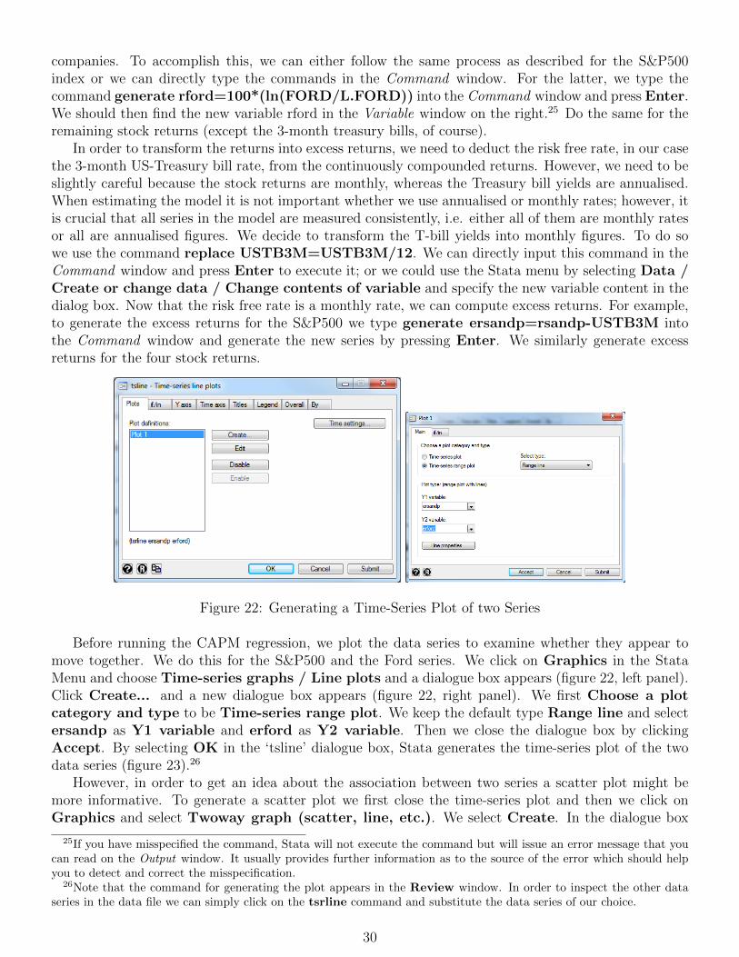
Before running the CAPM regression, we plot the data series to examine whether they appear tomove together. We do this for the S&P500 and the Ford series. We click on Graphics in the StataMenu and choose Time-series graphs / Line plots and a dialogue box appears (figure 22, left panel).Click Create... and a new dialogue box appears (figure 22, right panel). We first Choose a plotcategory and type to be Time-series range plot. We keep the default type Range line and selectersandp as Y1 variable and erford as Y2 variable. Then we close the dialogue box by clickingAccept. By selecting OK in the ‘tsline’ dialogue box, Stata generates the time-series plot of the twodata series (figure 23).26

However, in order to get an idea about the association between two series a scatter plot might bemore informative. To generate a scatter plot we first close the time-series plot and then we click onGraphics and select Twoway graph (scatter, line, etc.). We select Create. In the dialogue box

25If you have misspecified the command, Stata will not execute the command but will issue an error message that youcan read on the Output window. It usually provides further information as to the source of the error which should helpyou to detect and correct the misspecification.

26Note that the command for generating the plot appears in the Review window. In order to inspect the other dataseries in the data file we can simply click on the tsrline command and substitute the data series of our choice.

30

Figure 23: Time-Series Plot of two Series

that appears, we specify the following graph characteristics: We keep the default options Basic plotsand Scatter and select erford as Y variable and ersandp as X variable (see the input in figure 24,left panel).

Figure 24: Generating a Scatter Plot of two Series

We press Accept and OK and Stata generates a scatter plot of the excess S&P500 return and theexcess Ford return as depicted in figure 24, right panel. We see from this scatter plot that there appearsto be a weak association between ‘ersandp’ and ‘erford’. We can also create similar scatter plots for theother data series and the S&P500. Once finished, we just close the window of the graph.

To estimate the CAPM equation, we click on Statistics and then Linear models and relatedand Linear regression so that the familiar dialogue window ‘regress - Linear regression’ appears.

For the case of the Ford stock, the CAPM regression equation takes the form

(RFord − rf )t = α + β(RM − rf )t + ut

Thus, the dependent variable (y) is the excess return of Ford ‘rspot’ and it is regressed on a constant as

31

Figure 25: Estimating the CAPM Regression Equation

well as the excess market return ‘ersandp’.27 Once you have specified the variables, the dialogue windowshould resemble figure 25. To estimate the equation press OK. The results appear in the Outputwindow as below. Take a couple of minutes to examine the results of the regression. What is theslope coefficient estimate and what does it signify? Is this coefficient statistically significant? The betacoefficient (the slope coefficient) estimate is 2.026 with a t-ratio of 8.52 and a corresponding p-valueof 0.000. This suggests that the excess return on the market proxy has highly significant explanatorypower for the variability of the excess return of Ford stock. Let us turn to the intercept now. What isthe interpretation of the intercept estimate? Is it statistically significant? The α estimate is -0.320 witha t-ratio of -0.29 and a p-value of 0.769. Thus, we cannot reject that the α estimate is different from 0,indicating that the Ford stock does not seem to significantly outperform or under-perform the overallmarket..

regress erford ersandpSource SS df MS Number of obs = 135

F( 1, 133) = 72.64Model 11565.9116 1 11565.9116 Prob > F = 0.0000

Residual 21177.5644 133 159.229808 R-squared = 0.3532Adj R-squared = 0.3484

Total 32743.476 134 244.354298 Root MSE = 12.619

erford Coef. Std. Err. t P>|t| [95% Conf. Interval]ersandp 2.026213 .2377428 8.52 0.00 1.555967 2.496459

cons -.3198632 1.086409 -0.29 0.769 -2.468738 1.829011

.

Assume we want to test that the value of the population coefficient on ‘ersandp’ is equal to 1.How can we achieve this? The answer is to click on Statistics / Postestimation to launch Tests,contrasts, and comparisons of parameter estimates / Linear tests of parameter estimatesand then specify Test type: Linear expressions are equal and Coefficient: ersandp. Finally,

27Remember that the Stata command regress automatically includes a constant in the regression; thus, we do not needto manually include it among the independent variables.

32

we need to define the linear expression: ersandp=1.28 By clicking OK the F -statistics for thishypothesis test appears in the Output window. The F -statistic of 18.63 with a corresponding p-valueof 0 (at least up to the fourth decimal point) implying that the null hypothesis that the CAPM beta ofFord stock is 1 is convincingly rejected and hence the estimated beta of 2.026 is significantly differentfrom 1.29

28Alternatively, just type test (ersandp=1) into the Command window and press Enter.29This is hardly surprising given the distance between 1 and 2.026. However, it is sometimes the case, especially if

the sample size is quite small and this leads to large standard errors, that many different hypotheses will all result innon-rejection – for example, both H0 : β = 0 and H0 : β = 1 not rejected.

33

6 Sample output for multiple hypothesis tests

Brooks (2014, section 4.5)This example uses the ‘capm.dta’ workfile constructed in the previous section. So in case you are

starting a new session, re-load the Stata workfile and re-estimate the CAPM regression equation for theFord stock.30 If we examine the regression F -test, this also shows that the regression slope coefficientis not significantly different from zero, which in this case is exactly the same result as the t-test for thebeta coefficient (since there is only one slope coefficient). Thus, in this instance, the F -test statistic isequal to the square of the slope t-ratio.

Now suppose that we wish to conduct a joint test that both the intercept and slope parametersare one. We would perform this test in a similar way to the test involving only one coefficient. First,we launch the ‘Postestimation Selector’ by selecting Statistics / Postestimation. To open the spec-ification window for the Wald test we choose Tests, contrasts, and comparisons of parameterestimates / Linear tests of parameter estimates. We Create... the first restriction by selectingthe option Linear expressions are equal and as linear expression we specify ersandp=1. We clickOK. This is the first specification. In order to add the second specification, i.e. the coefficient on theconstant is 1 as well, we click on Create... again. In the Specification 2 dialogue box that appearswe select the Test type:Linear expressions are equal and specify the following linear expressioncons=1 in the dialog box. Once we have defined both specifications we click OK to generate theF -test statistics.31

In the Output window, Stata produces the familiar output for the F -test. However, we note that thejoint hypothesis test is indicated by the two conditions that are stated, ‘( 1) ersandp = 1’ and in thenext row ‘( 2) cons = 1’. Looking at the value of the F -statistic of 9.92 with a corresponding p-valueof 0.0001, we conclude that the null hypothesis, H0 : β1 = 1 and β2 = 1, is strongly rejected at the 1%significance level.

30To estimate the regression use the command regress erford ersandp.31You can also execute this command using the command line. You would use the command test (ersandp=1)

( cons=1). Note that it is important to set the parentheses around each of the terms as otherwise Stata will not executethe command and produce an error message.

34

7 Multiple regression using an APT-style model

Brooks (2014, section 4.6)The following example will show how we can extend the linear regression model introduced in the

previous sections to estimate multiple regressions in Stata. In the spirit of arbitrage pricing theory(APT), we will examine regressions that seek to determine whether the monthly returns on Microsoftstock can be explained by reference to unexpected changes in a set of macroeconomic and financialvariables. For this we rely on the dataset ‘macro.xls’ which contains 13 data series of financial andeconomic variables as well as a date variable spanning the time period from March 1986 until April 2013(i.e. 254 monthly observations for each of the series). In particular, the set of financial and economicvariables comprises the Microsoft stock price, the S&P500 index value, the consumer price index, anindustrial production index, Treasury bill yields for the following maturities: three months, six months,one year, three years, five years and ten years, a measure of ‘narrow’ money supply, a consumer creditse,ries, and a ‘credit spread’ series. The latter is defined as the difference in annualised average yieldsbetween a portfolio of bonds rated AAA and a portfolio of bonds rated BAA.

Before we can start with our analysis we need to import the dataset ‘macro.xls’ into Stata andadjust the ‘Date’ variable according to the steps outlined in previous sections.32 As Stata does not allowvariable names to have blanks, it automatically deletes them, e.g. the variable ‘Industrial Production’from the Excel workfile has been renamed by Stata to ‘Industrialproduction’. Remember to Save theworkfile as ‘macro.dta’.

Now that we have prepared our dataset we can start with the actual analysis. The first stage is togenerate a set of changes or differences for each of the variables, since the APT posits that the stockreturns can be explained by reference to the unexpected changes in the macroeconomic variables ratherthan their levels. The unexpected value of a variable can be defined as the difference between theactual (realised) value of the variable and its expected value. The question then arises about how webelieve that investors might have formed their expectations, and while there are many ways to constructmeasures of expectations, the easiest is to assume that investors have naive expectations that the nextperiod value of the variable is equal to the current value. This being the case, the entire change in thevariable from one period to the next is the unexpected change (because investors are assumed to expectno change).33

To transform the variables, we either use the Stata Menu ((Data / Create or change data /Create new variable)) or we directly type the commands into the Command window:

generate dspread=BAAAAASPREAD-L.BAAAAASPREADgenerate dcredit=CONSUMERCREDIT-L.CONSUMERCREDITgenerate dprod=Industrialproduction-L.Industrialproductiongenerate rmsoft=100*(ln(Microsoft/L.Microsoft))generate rsandp=100*(ln(SANDP/L.SANDP))generate dmoney=M1MONEYSUPPLY-L.M1MONEYSUPPLYgenerate inflation=100*(ln(CPI/L.CPI))generate term=USTB10Y-USTB3M

and press Enter to execute them. Next we need to apply further transformations to some of thetransformed series, so we generate another set of variables:

32Recall that we first need to transform the Date type from daily to monthly with replace Date=mofd(Date). Thenwe format the Date variable into human-readable format with format Date %tm. Finally, we define the time variableusing tsset Date.

33It is an interesting question as to whether the differences should be taken on the levels of the variables or theirlogarithms. If the former, we have absolute changes in the variables, whereas the latter would lead to proportionatechanges. The choice between the two is essentially an empirical one, and this example assumes that the former is chosen,apart from for the stock price series themselves and the consumer price series.

35

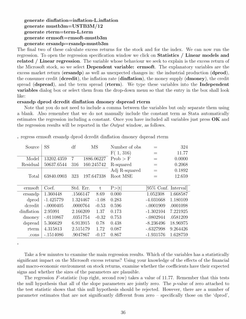
generate dinflation=inflation-L.inflationgenerate mustb3m=USTB3M/12generate rterm=term-L.termgenerate ermsoft=rmsoft-mustb3mgenerate ersandp=rsandp-mustb3m

The final two of these calculate excess returns for the stock and for the index. We can now run theregression. To open the regression specification window we click on Statistics / Linear models andrelated / Linear regression. The variable whose behaviour we seek to explain is the excess return ofthe Microsoft stock, so we select Dependent variable: ermsoft. The explanatory variables are theexcess market return (ersandp) as well as unexpected changes in: the industrial production (dprod),the consumer credit (dcredit), the inflation rate (dinflation), the money supply (dmoney), the creditspread (dspread), and the term spread (rterm). We type these variables into the Independentvariables dialog box or select them from the drop-down menu so that the entry in the box shall looklike:ersandp dprod dcredit dinflation dmoney dspread rterm

Note that you do not need to include a comma between the variables but only separate them usinga blank. Also remember that we do not manually include the constant term as Stata automaticallyestimates the regression including a constant. Once you have included all variables just press OK andthe regression results will be reported in the Output window, as follows.

. regress ermsoft ersandp dprod dcredit dinflation dmoney dspread rterm

Source SS df MS Number of obs = 324F( 1, 316) = 11.77

Model 13202.4359 7 1886.06227 Prob > F = 0.0000Residual 50637.6544 316 160.245742 R-squared = 0.2068

Adj R-squared = 0.1892Total 63840.0903 323 197.647338 Root MSE = 12.659

ermsoft Coef. Std. Err. t P>|t| [95% Conf. Interval]ersandp 1.360448 .1566147 8.69 0.000 1.052308 1.668587

dprod -1.425779 1.324467 -1.08 0.283 -4.031668 1.180109dcredit -.0000405 .0000764 -0.53 0.596 -.0001909 .0001098

dinflation 2.95991 2.166209 1.37 0.173 -1.302104 7.221925dmoney -.0110867 .0351754 -0.32 0.753 -.0802944 .0581209dspread 5.366629 6.913915 0.78 0.438 -8.236496 18.96975

rterm 4.315813 2.515179 1.72 0.087 -.6327998 9.264426cons -.1514086 .9047867 -0.17 0.867 -1.931576 1.628759

.

Take a few minutes to examine the main regression results. Which of the variables has a statisticallysignificant impact on the Microsoft excess returns? Using your knowledge of the effects of the financialand macro-economic environment on stock returns, examine whether the coefficients have their expectedsigns and whether the sizes of the parameters are plausible.

The regression F -statistic (top right, second row) takes a value of 11.77. Remember that this teststhe null hypothesis that all of the slope parameters are jointly zero. The p-value of zero attached tothe test statistic shows that this null hypothesis should be rejected. However, there are a number ofparameter estimates that are not significantly different from zero – specifically those on the ‘dprod’,

36

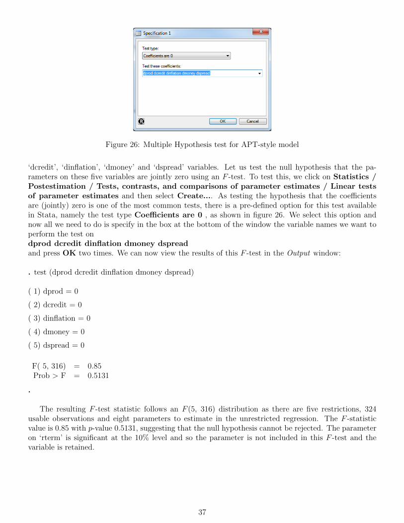
Figure 26: Multiple Hypothesis test for APT-style model

‘dcredit’, ‘dinflation’, ‘dmoney’ and ‘dspread’ variables. Let us test the null hypothesis that the pa-rameters on these five variables are jointly zero using an F -test. To test this, we click on Statistics /Postestimation / Tests, contrasts, and comparisons of parameter estimates / Linear testsof parameter estimates and then select Create.... As testing the hypothesis that the coefficientsare (jointly) zero is one of the most common tests, there is a pre-defined option for this test availablein Stata, namely the test type Coefficients are 0 , as shown in figure 26. We select this option andnow all we need to do is specify in the box at the bottom of the window the variable names we want toperform the test ondprod dcredit dinflation dmoney dspreadand press OK two times. We can now view the results of this F -test in the Output window:

. test (dprod dcredit dinflation dmoney dspread)

( 1) dprod = 0

( 2) dcredit = 0

( 3) dinflation = 0

( 4) dmoney = 0

( 5) dspread = 0

F( 5, 316) = 0.85Prob > F = 0.5131

.

The resulting F -test statistic follows an F (5, 316) distribution as there are five restrictions, 324usable observations and eight parameters to estimate in the unrestricted regression. The F -statisticvalue is 0.85 with p-value 0.5131, suggesting that the null hypothesis cannot be rejected. The parameteron ‘rterm’ is significant at the 10% level and so the parameter is not included in this F -test and thevariable is retained.

37

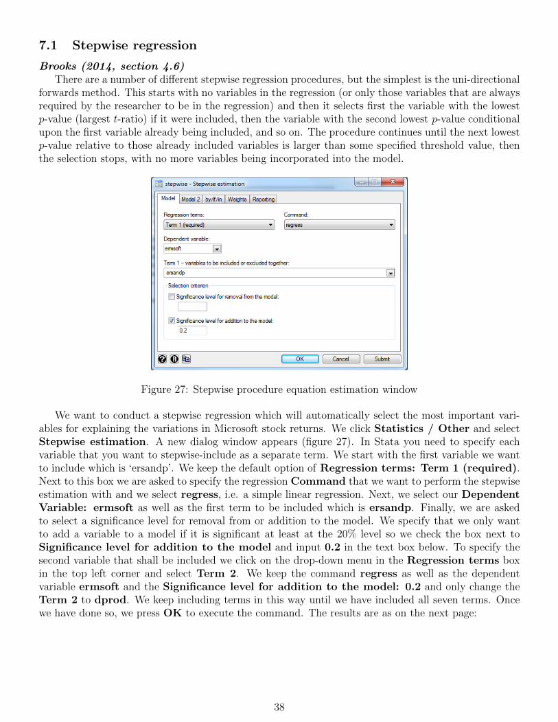
7.1 Stepwise regression

Brooks (2014, section 4.6)There are a number of different stepwise regression procedures, but the simplest is the uni-directional

forwards method. This starts with no variables in the regression (or only those variables that are alwaysrequired by the researcher to be in the regression) and then it selects first the variable with the lowestp-value (largest t-ratio) if it were included, then the variable with the second lowest p-value conditionalupon the first variable already being included, and so on. The procedure continues until the next lowestp-value relative to those already included variables is larger than some specified threshold value, thenthe selection stops, with no more variables being incorporated into the model.

Figure 27: Stepwise procedure equation estimation window

We want to conduct a stepwise regression which will automatically select the most important vari-ables for explaining the variations in Microsoft stock returns. We click Statistics / Other and selectStepwise estimation. A new dialog window appears (figure 27). In Stata you need to specify eachvariable that you want to stepwise-include as a separate term. We start with the first variable we wantto include which is ‘ersandp’. We keep the default option of Regression terms: Term 1 (required).Next to this box we are asked to specify the regression Command that we want to perform the stepwiseestimation with and we select regress, i.e. a simple linear regression. Next, we select our DependentVariable: ermsoft as well as the first term to be included which is ersandp. Finally, we are askedto select a significance level for removal from or addition to the model. We specify that we only wantto add a variable to a model if it is significant at least at the 20% level so we check the box next toSignificance level for addition to the model and input 0.2 in the text box below. To specify thesecond variable that shall be included we click on the drop-down menu in the Regression terms boxin the top left corner and select Term 2. We keep the command regress as well as the dependentvariable ermsoft and the Significance level for addition to the model: 0.2 and only change theTerm 2 to dprod. We keep including terms in this way until we have included all seven terms. Oncewe have done so, we press OK to execute the command. The results are as on the next page:

38

. stepwise, pe(0.2) : regress ermsoft (ersandp) (dprod) (dcredit) (dinflation) (dmoney) (dspread) (rterm)

begin with empty modelp = 0.0000 < 0.2000 adding ersandpp = 0.0950 < 0.2000 adding rtermp = 0.1655 < 0.2000 adding dinflation

Source SS df MS Number of obs = 324F( 3, 320) = 26.82

Model 12826.9936 3 4275.66453 Prob > F = 0.0000Residual 51013.0967 320 159.415927 R-squared = 0.2009

Adj R-squared = 0.1934Total 63840.0903 323 197.647338 Root MSE = 12.626

ermsoft Coef. Std. Err. t P>|t| [95% Conf. Interval]ersandp 1.338211 .1530557 8.74 0.000 1.037089 1.639334

rterm 4.369891 2.49711 1.75 0.81 -.5429353 9.282718dinflation 2.876958 2.069933 1.39 0.166 -1.195438 6.949354

cons -.6873412 .7027164 -0.98 0.329 -2.069869 .6951865

.

Note that a stepwise regression can be executed in different ways, e.g. either ‘forward’ or ‘backward’.‘Forward’ will start with the list of required regressors (the intercept only in this case) and will sequen-tially add to them, while ‘backward’ will start by including all of the variables and will sequentiallydelete variables from the regression. The way we have specified our stepwise estimation we performa ‘forward’-selection estimation and only add a variable to the model if it is significant at the 20%significance level, or higher.34

Turning to the results of the step-wise estimation, we find that the excess market return, the termstructure, and unexpected inflation variables have been included, while the money supply, default spreadand credit variables have been omitted.

34We will not perform a backward-selection estimation. For details on the backward specification please refer to thechapter on stepwise in the Stata Manual.

39

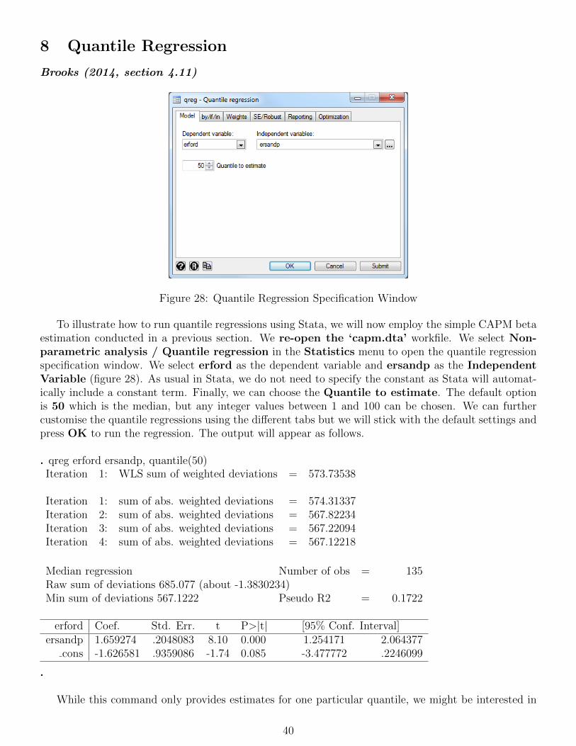
8 Quantile Regression

Brooks (2014, section 4.11)

Figure 28: Quantile Regression Specification Window

To illustrate how to run quantile regressions using Stata, we will now employ the simple CAPM betaestimation conducted in a previous section. We re-open the ‘capm.dta’ workfile. We select Non-parametric analysis / Quantile regression in the Statistics menu to open the quantile regressionspecification window. We select erford as the dependent variable and ersandp as the IndependentVariable (figure 28). As usual in Stata, we do not need to specify the constant as Stata will automat-ically include a constant term. Finally, we can choose the Quantile to estimate. The default optionis 50 which is the median, but any integer values between 1 and 100 can be chosen. We can furthercustomise the quantile regressions using the different tabs but we will stick with the default settings andpress OK to run the regression. The output will appear as follows.

. qreg erford ersandp, quantile(50)Iteration 1: WLS sum of weighted deviations = 573.73538

Iteration 1: sum of abs. weighted deviations = 574.31337Iteration 2: sum of abs. weighted deviations = 567.82234Iteration 3: sum of abs. weighted deviations = 567.22094Iteration 4: sum of abs. weighted deviations = 567.12218

Median regression Number of obs = 135Raw sum of deviations 685.077 (about -1.3830234)Min sum of deviations 567.1222 Pseudo R2 = 0.1722

erford Coef. Std. Err. t P>|t| [95% Conf. Interval]ersandp 1.659274 .2048083 8.10 0.000 1.254171 2.064377

cons -1.626581 .9359086 -1.74 0.085 -3.477772 .2246099

.

While this command only provides estimates for one particular quantile, we might be interested in

40

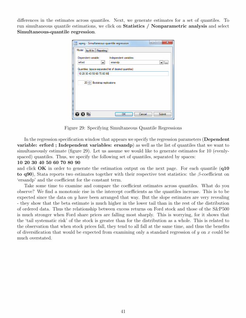
differences in the estimates across quantiles. Next, we generate estimates for a set of quantiles. Torun simultaneous quantile estimations, we click on Statistics / Nonparametric analysis and selectSimultaneous-quantile regression.

Figure 29: Specifying Simultaneous Quantile Regressions

In the regression specification window that appears we specify the regression parameters (Dependentvariable: erford ; Independent variables: ersandp) as well as the list of quantiles that we want tosimultaneously estimate (figure 29). Let us assume we would like to generate estimates for 10 (evenly-spaced) quantiles. Thus, we specify the following set of quantiles, separated by spaces:10 20 30 40 50 60 70 80 90and click OK in order to generate the estimation output on the next page. For each quantile (q10to q90), Stata reports two estimates together with their respective test statistics: the β-coefficient on‘ersandp’ and the coefficient for the constant term.

Take some time to examine and compare the coefficient estimates across quantiles. What do youobserve? We find a monotonic rise in the intercept coefficients as the quantiles increase. This is to beexpected since the data on y have been arranged that way. But the slope estimates are very revealing- they show that the beta estimate is much higher in the lower tail than in the rest of the distributionof ordered data. Thus the relationship between excess returns on Ford stock and those of the S&P500is much stronger when Ford share prices are falling most sharply. This is worrying, for it shows thatthe ‘tail systematic risk’ of the stock is greater than for the distribution as a whole. This is related tothe observation that when stock prices fall, they tend to all fall at the same time, and thus the benefitsof diversification that would be expected from examining only a standard regression of y on x could bemuch overstated.

41

. sqreg erford ersandp, quantiles(10 20 30 40 50 60 70 80 90) reps(20)(fitting base model)

Bootstrap replications (20)—+— 1 —+— 2 —+— 3 —+— 4 —+— 5....................

Simultaneous quantile regression Number of obs = 135bootstrap(20) SEs .10 Pseudo R2 = 0.2198

.20 Pseudo R2 = 0.1959

.30 Pseudo R2 = 0.1911

.40 Pseudo R2 = 0.1748

.50 Pseudo R2 = 0.1722

.60 Pseudo R2 = 0.1666

.70 Pseudo R2 = 0.1512

.80 Pseudo R2 = 0.1299

.90 Pseudo R2 = 0.1302

Bootstraperford Coef. Std. Err. t P>|t| [95% Conf. Interval]

q10ersandp 2.399342 .7992684 3.00 0.003 .8184205 3.980264

cons -12.42521 1.7106095 -7.26 0.000 -15.80873 -9.041696q20

ersandp 1.845833 .4081245 4.52 0.000 1.03858 2.653087cons -8.294803 1.147304 5 -7.23 0.000 -10.56413 -6.025481

q30ersandp 1.599782 .28628845 5.59 0.000 1.033514 2.166049

cons -5.592711 1.0530095 -5.31 0.000 -7.675521 -3.5099q40

ersandp 1.670869 .2012385 8.30 0.000 1.272828 2.06891cons -4.294994 1.1826925 -3.63 0.000 -6.634313 -1.955676

q50ersandp 1.659274 .23184355 7.16 0.000 1.200696 2.117851

cons -1.626581 .80365515 -2.02 0.045 -3.21618 -.0369823q60

ersandp 1.767672 .24468975 7.22 0.000 1.283685 2.251658cons 1.039469 .86143185 1.21 0.230 -.6644094 2.743348

q70ersandp 1.652457 .26588865 6.21 0.000 1.12654 2.178374

cons 2.739059 .93780645 2.92 0.004 .884114 4.594003q80

ersandp 1.970517 .38994735 5.05 0.000 1.199216 2.741818cons 7.115613 1.8265115 3.90 0.000 3.502844 10.72838

q90ersandp 1.615322 .55686645 2.90 0.004 .5138614 2.716782

cons 14.43761 2.163004 5 6.67 0.000 10.15927 18.71594

.

42

Figure 30: Equality of Quantile Estimates

Several diagnostics and specification tests for quantile regressions may be computed, and one of par-ticular interest is whether the coefficients for each quantile can be restricted to be the same. To performthe equality test we rely on the test command that we have used in previous sections for testing linearhypotheses. It can be accessed via Statistics / Postestimation / Tests, contrasts, and compar-isons of parameter estimates / Linear tests of parameter estimates. Note that it is importantthat the last estimation that you performed was the simultaneous quantile regression as Stata alwaysperforms hypothesis tests based on the most recent estimates. In the test specification window we clickCreate... and choose the test type Linear expressions are equal (figure 30, upper panel). We clickon the drop-down menu for Coefficient and select q10:ersandp, where [q10] indicates the coefficientestimate from the regression based on the 10th quantile. Then we press Add and the coefficient estimatefor ‘q10:ersandp’ appears in the ‘Linear expression’ box at the bottom. Next we select q20:ersandpand also Add this variable to the ‘Linear expression’. Note that Stata automatically adds an ‘equal’sign between the two parameters. We keep doing this until we have included all 9 quantile estimatesfor ‘ersandp’ in the ‘Linear expression’. Then we click OK and we see that expression appears at thebottom of the ‘test’ specification window (figure 30, lower panel). Clicking OK again generates thefollowing test results.

43

. test ( b[q10:ersandp] = b[q20:ersandp]= b[q30:ersandp]= b[q40:ersandp]= b[q50:ersandp]=b[q60:ersandp]= b[q70:ersandp]= b[q80:ersandp]= b[q90:ersandp])

( 1) [q10]ersandp - [q20]ersandp = 0

( 2) [q10]ersandp - [q30]ersandp = 0

( 3) [q10]ersandp - [q40]ersandp = 0

( 4) [q10]ersandp - [q50]ersandp = 0

( 5) [q10]ersandp - [q60]ersandp = 0

( 6) [q10]ersandp - [q70]ersandp = 0

( 7) [q10]ersandp - [q80]ersandp = 0

( 8) [q10]ersandp - [q90]ersandp = 0

F( 8, 133) = 1.58Prob > F = 0.1375

.

We see that Stata has rearranged our initial test equation to express it in a way that makes it easierfor the program to execute the command. The rearrangement is innocuous and, in fact, allows Stata toperform fairly complicated algebraic restrictions. In our case, we see that the test whether all coefficientsare equal is the same as testing whether the difference between the coefficient on ‘ersand’ for quantile10 and the respective coefficient for each of the other quantiles is zero.35 Turning to the test-statistic wefind that the F -value is 1.58 with a p-value of 0.1375. In other words, we cannot reject the hypothesisthat all coefficient estimates are equal, although the F -statistic is close to being significant at the 10%level. If we would have found that the coefficient estimates across quaniltes was not equal, this wouldhave implied that the association between the excess returns of Ford stock and the S&P500 index wouldvary depending on the part of the return distribution we are looking at, i.e. whether we are looking atvery negative or very positive excess returns.

35To see that this is the case let us do some simple rearrangements. If all coefficients are equal then it has to bethe case that individual pairs of the set of coefficients are equal to one another, i.e. [q10]ersandp=[q20]ersandp and[q10]ersandp=[q30]ersandp etc. However, if the previous two equations are true, i.e. both [q20]ersandp and [q30]ersandpare equal to [q10]ersandp, then this implies that [q20]ersandp=[q30]ersandp. Thus, in order to test the equality of allcoefficients to each other it is sufficient to test that all coefficients are equal to one specific coefficient,e.g. [q10]ersand.Now, we can rearrange pairwise equalities by expression them as differences as [q10]ersandp=[q20]ersandp is the same aswriting [q10]ersandp-[q20]ersandp=0.

44

9 Calculating principal component

Brooks (2014, appendix 4.2)

Figure 31: Principal Component Analysis Specification Window

In this section we will examine a set of interest rates of different maturities and calculate the principalcomponents for this set of variables in Stata. First we re-open the ‘macro.dta’ workfile which containsUS Treasury bill and bond series of various maturities. Next we click on Statistics in the Statamenu and select Multivariate analysis / Factor and principal component analysis / Principalcomponent analysis (PCA). A new window appears where we are asked to input the Variables forwhich we want to generate principal components (figure 31). We type in the six treasury bill ratesUSTB3M USTB6M USTB1Y USTB3Y USTB5Y USTB10Yand click OK. Note that there are multiple ways to customise the principal component analysis usingthe options in the tabs. However, we keep the default settings for now. The results are presented in theOutput window, as shown below. The first panel lists the eigenvalues of the correlation matrix, orderedfrom largest to smallest; the second panel reports the corresponding eigenvectors.

. pca USTB3M USTB6M USTB1Y USTB3Y USTB5Y USTB10Y

Principal components/correlation Number of obs = 326Number of comp. = 6Trace = 6

Rotation: (unrotated = principal) Rho = 1.0000

Component Eigenvalue Difference Proportion CumulativeComp1 5.79174 5.59442 0.9653 0.9653Comp2 .19732 .189221 0.0329 0.9982Comp3 .00809953 .00586455 0.0013 0.9995Comp4 .00223498 .00183054 0.0004 0.9999Comp5 .000404434 .000202525 0.0001 1.0000Comp6 .000201909 . 0.0000 1.0000

45

Principal components (eigenvectors)

Variable Comp1 Comp2 Comp3 Comp4 Comp5 Comp6 UnexplainedUSTB3M 0.4066 -0.4482 0.5146 -0.4607 0.3137 -0.2414 0

UUSTB6M 0.4090 -0.3963 0.1014 0.1983 -0.4987 0.6143 0USTB1Y 0.4121 -0.2713 -0.3164 0.5988 0.0591 -0.5426 0USTB3Y 0.4144 0.1176 -0.5612 -0.2183 0.5394 0.4010 0USTB5Y 0.4098 0.3646 -0.2212 -0.4656 -0.5761 -0.3185 0

USTB10Y 0.3973 0.6493 0.5107 0.3542 0.1627 0.0878 0

.

It is evident that there is a great deal of common variation in the series, since the first principalcomponent captures over 96% of the variation in the series and the first two components capture 99.8%.Consequently, if we wished, we could reduce the dimensionality of the system by using two componentsrather than the entire six interest rate series. Interestingly, the first component comprises almost exactlyequal weights in all six series while the second component puts a larger negative weight on the shortestyield and gradually increasing weights thereafter. This ties in with the common belief that the firstcomponent captures the level of interest rates, the second component captures the slope of the termstructure (and the third component captures curvature in the yield curve).

46

10 Diagnostic testing

10.1 Testing for heteroscedasticity

Brooks (2014, section 5.4)In this example we will undertake a test for heteroscedasticity in Stata, using the ‘macro.dta’ workfile.

We will inspect the residuals of the APT-style regression of the excess return of Ford stock, ‘erford’,on unexpected changes in a set of financial and macroeconomic variables, which we have estimatedabove. Thus, the first step is to reproduce the regression results. The simplest way is to re-estimate theregression by typing the commandregress ermsoft ersandp dprod dcredit dinflation dmoney dspread rtermin the Command window and press Enter. This time we are less interested in the coefficient estimatesreported in the Output window, but we focus on the properties of the residuals from this regression.To get a first impression about the properties of the residuals we want to plot them. When Stataperforms an estimation it keeps specific estimates in its memory which can then be used in postestimationanalysis; among them the residuals of a regression. To obtain the residuals we use the command predictwhich allows us to create a variable of the predicted variables in memory.36 We click on Statistics /Postestimation and in the ‘Postestimation Selector’ we select Predictions and Predictions andtheir SEs, leverage statistics, distance statistics, etc. (figure 32).

Figure 32: Postestimation Selector for Predictions

In the ‘predict’ specification window that appears we name the residual series we want to generatein the New variable name: box as resid and select the option Residuals (equation-level scores)which specifies that the new ‘resid’ series shall contain the (unadjusted) residuals (figure 33). By pressingOK we should find that the variable ‘resid’ now appears as a new variable in the Variables window.

To plot this series we simply select Graphics / Time-series graphs / Line plots, click onCreate... and in the new window we select resid as the Y Variable. Clicking Accept and then OK

36For more information about the functionalities of predict please refer to the respective entry in the Stata Manual.

47

Figure 33: Obtaining Residuals using predict

should generate a time-series plot of the residual series, similar to figure 34.37

Let us examine the pattern of residuals over time. If the residuals of the regression have systematicallychanging variability over the sample, that is a sign of heteroscedasticity. In this case, it is hard to seeany clear pattern (although it is interesting to note the considerable reduction in volatility post-2003),so we need to run the formal statistical test.

Figure 34: Time series Plot of Residuals

37Alternatively, you can directly use the command twoway (tsline resid) to generate the residual plot, after havinggenerated the ‘resid’ series using the command predict resid, residuals.

48

Figure 35: Postestimation Selector for Heteroscedasticity Tests

To do so we click on Statistics / Postestimation and then select Specification, diagnostic,and goodness-of-fit analysis / Tests for heteroskedasticity (figure 35). In the ‘estat’ specificationwindow, we are first asked to select the type of Reports and statistics (subcommand) as in figure36. The default option is Tests for heteroskedasticity (hettest) which is exactly the commandthat we are looking for; thus we do not make any changes at this stage. Next we specify the type ofheteroscedasticity test to compute using the drop-down menu next to Test to compute. We can choosebetween three options: (1) the (original) Breusch-Pagan/Cook-Weisberg test, which assumes thatthe regression disturbances are normally distributed; (2) the N*R2 version of the score test thatdrops the normality assumption; (3) the F-statistic version which also drops the normality assumption.Let us start by selecting the Breusch-Pagan/Cook-Weisberg test. Clicking OK will generate thetest statistics in the Output window on the following page. As you can see the null hypothesis is one ofconstant variance, i.e. homoscedasticity. With a χ2-value of 0.11 and a corresponding p-value of 0.7378,the Beusch-Pagan/Cook-Weisberg test suggests that we cannot reject the null hypothesis of constantvariance of the residuals. To test the robustness of this result to alternative distributional assumptions,we can also run the other two test types. Below is the output for all three tests. As you can see fromthe test statistics and p-values, all tests lead to the conclusion that there does not seem to be a seriousproblem of heteroscedastic errors for our APT-style model.

49

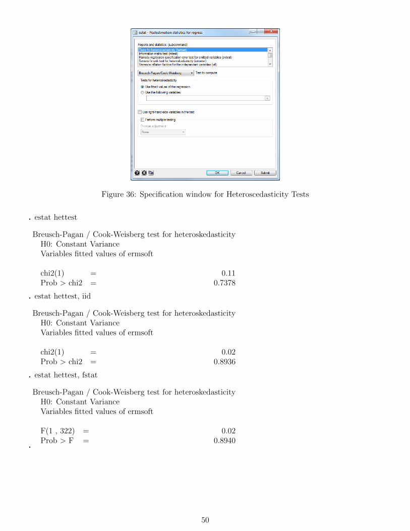
Figure 36: Specification window for Heteroscedasticity Tests

. estat hettest

Breusch-Pagan / Cook-Weisberg test for heteroskedasticityH0: Constant VarianceVariables fitted values of ermsoft

chi2(1) = 0.11Prob > chi2 = 0.7378

. estat hettest, iid

Breusch-Pagan / Cook-Weisberg test for heteroskedasticityH0: Constant VarianceVariables fitted values of ermsoft

chi2(1) = 0.02Prob > chi2 = 0.8936

. estat hettest, fstat

Breusch-Pagan / Cook-Weisberg test for heteroskedasticityH0: Constant VarianceVariables fitted values of ermsoft

F(1 , 322) = 0.02Prob > F = 0.8940

.

50

10.2 Using White’s modified standard error estimates

We can specify to estimate the regression with heteroscedasticity-robust standard errors in Stata. Whenwe open the regress specification window we see different tabs. So far we have only focused on theModel tab that specifies the dependent and independent variables. If we move to the SE/Robust tab,we are presented with different options for adjusting the standard errors (figure 37).

Figure 37: Adjusting Standard Errors for OLS Regressions

In order to obtain standard errors that are robust to heteroscedasticity we select the option Robust.Beneath the selection box, three Bias correction options appear. We keep the default option.38

Comparing the regression output for our APT-style model using robust standard errors with that usingordinary standard errors, we find that the changes in significance are only marginal, as shown in theoutput below.

Of course, only the standard errors have changed and the parameter estimates remain identical tothose estimated before. The heteroscedasticity-consistent standard errors are smaller for all variables,resulting in t-ratios growing in absolute value and p-values being smaller. The main changes in theconclusions reached are that the term structure variable, which was previously significant only at the10% level, is now significant at 5%, and the unexpected inflation and change in industrial productionvariables are now significant at the 10% level.

38Alternatively, you can directly adjust the estimation command in the Command window to account for robust standarderrors by adding ‘, vce(robust)’ at the end of the command, i.e. regress ermsoft ersandp dprod dcredit dinflation dmoneydspread rterm, vce(robust). For more information on the different standard error adjustments please refer to the entriesregress and vce option in the Stata Manual.

51

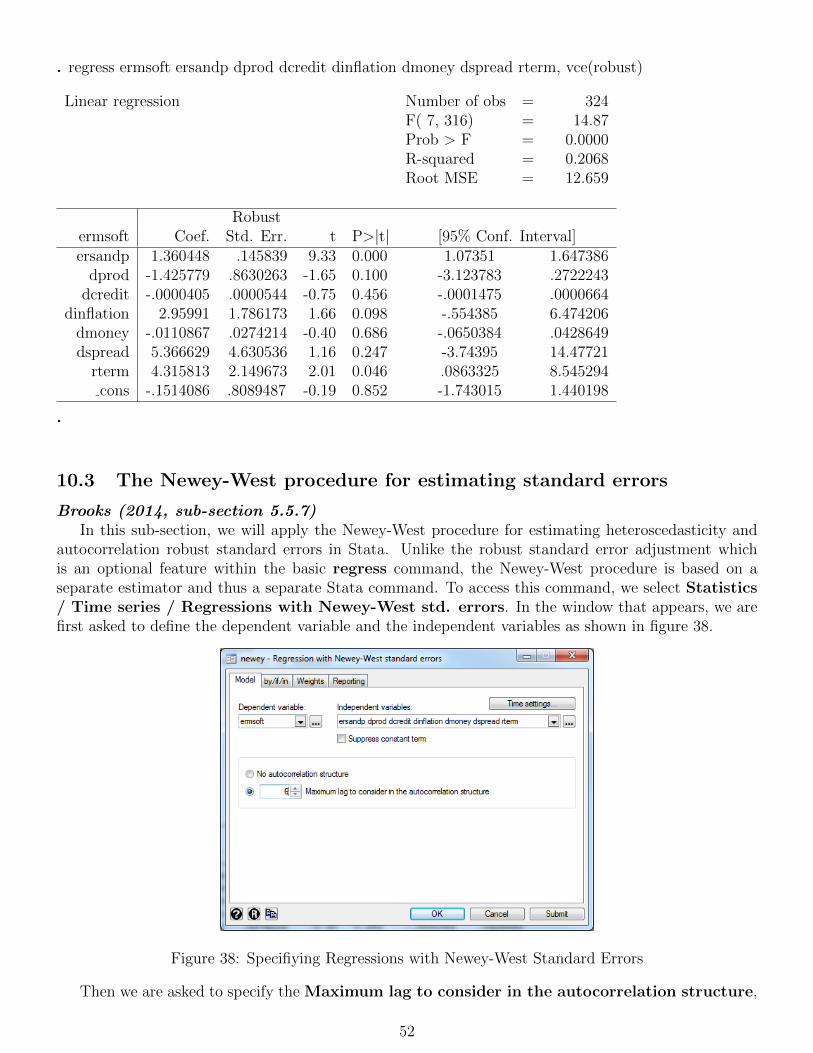
. regress ermsoft ersandp dprod dcredit dinflation dmoney dspread rterm, vce(robust)

Linear regression Number of obs = 324F( 7, 316) = 14.87Prob > F = 0.0000R-squared = 0.2068Root MSE = 12.659

Robustermsoft Coef. Std. Err. t P>|t| [95% Conf. Interval]ersandp 1.360448 .145839 9.33 0.000 1.07351 1.647386

dprod -1.425779 .8630263 -1.65 0.100 -3.123783 .2722243dcredit -.0000405 .0000544 -0.75 0.456 -.0001475 .0000664

dinflation 2.95991 1.786173 1.66 0.098 -.554385 6.474206dmoney -.0110867 .0274214 -0.40 0.686 -.0650384 .0428649dspread 5.366629 4.630536 1.16 0.247 -3.74395 14.47721

rterm 4.315813 2.149673 2.01 0.046 .0863325 8.545294cons -.1514086 .8089487 -0.19 0.852 -1.743015 1.440198

.

10.3 The Newey-West procedure for estimating standard errors

Brooks (2014, sub-section 5.5.7)In this sub-section, we will apply the Newey-West procedure for estimating heteroscedasticity and

autocorrelation robust standard errors in Stata. Unlike the robust standard error adjustment whichis an optional feature within the basic regress command, the Newey-West procedure is based on aseparate estimator and thus a separate Stata command. To access this command, we select Statistics/ Time series / Regressions with Newey-West std. errors. In the window that appears, we arefirst asked to define the dependent variable and the independent variables as shown in figure 38.

Figure 38: Specifiying Regressions with Newey-West Standard Errors

Then we are asked to specify the Maximum lag to consider in the autocorrelation structure,

52

i.e. we manually input the maximum number of lagged residuals that shall be considered for inclusionin the model. There might be different economic motivations for choosing the maximum lag length,depending on the specific analysis one is undertaking. In our example we decide to include a maximumlag length of six, implying that we assume that the potential autocorrelation in our data does not gobeyond the window of six months.39 By clicking OK, the following regression results appear in theOutput window.

. newey ermsoft ersandp dprod dcredit dinflation dmoney dspread rterm, lag(6)

Regression with Newey-West standard errors Number of obs = 324maximum lag: 6 F( 7, 316) = 14.89

Prob > F = 0.0000

Newey-Westermsoft Coef. Std. Err. t P>|t| [95% Conf. Interval]ersandp 1.360448 .1468384 9.26 0.000 1.071543 1.649352

dprod -1.425779 .7546947 -1.89 0.060 -2.910641 .059082dcredit -.0000405 .0000483 -0.84 0.402 -.0001355 .0000544

dinflation 2.95991 1.975182 1.50 0.135 -.9262584 6.846079dmoney -.0110867 .0292009 -0.38 0.704 -.0685394 .046366dspread 5.366629 4.57456 1.17 0.242 -3.633816 14.36707

rterm 4.315813 2.282997 1.89 0.060 -.1759814 8.807608cons -.1514086 .7158113 -0.21 0.833 -1.559767 1.25695

.

10.4 Autocorrelation and dynamic models

Brooks (2014, sub-section 5.5.12)In Stata, the lagged values of variables can be used as regressors or for other purposes by using

the notation L.x for a one-period lag, L5.x for a five-period lag, and so on, where x is the variablename. Stata will automatically adjust the sample period used for estimation to take into account theobservations that are lost in constructing the lags. For example, if the regression contains five lags ofthe dependent variable, five observations will be lost and estimation will commence with observationsix. Additionally, Stata also accounts for missing observations when using the time operator L. Note,however, that in order to use the time operator L. it is essential to set the time variable in the data setusing the command tsset.

In this section, we want to apply different tests for autocorrelation in Stata, using the APT-stylemodel of the previous section (‘macro.dta’ workfile).40

The simplest test for autocorrelation is due to Durbin and Watson (1951). It is a test for first-orderautocorrelation - i.e. it tests only for a relationship between an error and its immediately previousvalue. To access the Durbin-Watson (DW ) test, we access the ‘Postestimation Selector’ via Statistics/ Postestimation and then select Durbin-Watson d statistic to test for first-order serial corre-lation under the category Specification, diagnostic, and comparisons of parameter estimates(figure 39).

39Note that if we were to specify No autocorrelation structure the Newey-West adjusted standard errors would bethe same as the robust standard errors introduced in the previous section.

40Note that it is important that the last model you have estimated is regress ermsoft ersandp dprod dcredit

53

Figure 39: Postestimation Selector for the Durbin-Watson Test

Next we click OK as the correct option has already been pre-selected, i.e. Durbin-Watson dstatistic(dwatson - time series only). The following test results will appear in the Output window.

. estat dwatson

Durbin-Watson d-statistic( 8, 324) = 2.165384.

The value of the DW statistic is 2.165. What is the appropriate conclusion regarding the presenceor otherwise of first order autocorrelation in this case?

An alternative test for autocorrelation is the Breusch-Godfrey test. It is a more general test for auto-correlation than DW and allows to test for higher order autocorrelation. In Stata, the Breusch-Godfreytest can be conducted by selectingn Breusch-Godfrey test for higher-order serial correlation inthe ‘Postestimation Selector’. Again, the correct option Breusch-Godfrey test (bgodfrey - timeseries only) is pre-selected and we only need to Specify a list of lag orders to be tested. Assumingthat we select to employ 10 lags in the test, the results shall appear as below.

. estat bgodfrey, lags(10)

Breusch-Godfrey LM test for autocorrelation

lags(p) chi2 df Prob > chi210 22.623 10 0.0122

H0: no serial correlation

.

dinflation dmoney dspread rterm.

54

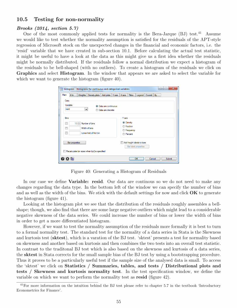
10.5 Testing for non-normality

Brooks (2014, section 5.7)One of the most commonly applied tests for normality is the Bera-Jarque (BJ) test.41 Assume

we would like to test whether the normality assumption is satisfied for the residuals of the APT-styleregression of Microsoft stock on the unexpected changes in the financial and economic factors, i.e. the‘resid’ variable that we have created in sub-section 10.1. Before calculating the actual test statistic,it might be useful to have a look at the data as this might give us a first idea whether the residualsmight be normally distributed. If the residuals follow a normal distribution we expect a histogram ofthe residuals to be bell-shaped (with no outliers). To create a histogram of the residuals we click onGraphics and select Histogram. In the window that appears we are asked to select the variable forwhich we want to generate the histogram (figure 40).

Figure 40: Generating a Histogram of Residuals

In our case we define Variable: resid. Our data are continous so we do not need to make anychanges regarding the data type. In the bottom left of the window we can specify the number of binsand as well as the width of the bins. We stick with the default settings for now and click OK to generatethe histogram (figure 41).

Looking at the histogram plot we see that the distribution of the residuals roughly assembles a bell-shape; though, we also find that there are some large negative outliers which might lead to a considerablenegative skewness of the data series. We could increase the number of bins or lower the width of binsin order to get a more differentiated histogram.

However, if we want to test the normality assumption of the residuals more formally it is best to turnto a formal normality test. The standard test for the normality of a data series in Stata is the Skewnessand kurtosis test (sktest), which is a varation of the BJ test. ‘sktest’ presents a test for normality basedon skewness and another based on kurtosis and then combines the two tests into an overall test statistic.In contrast to the traditonal BJ test which is also based on the skewness and kurtosis of a data series,the sktest in Stata corrects for the small sample bias of the BJ test by using a bootstrapping procedure.Thus it proves to be a particularly useful test if the sample size of the analysed data is small. To accessthe ‘sktest’ we click on Statistics / Summaries, tables, and tests / Distributional plots andtests / Skewness and kurtosis normality test. In the test specification window, we define thevariable on which we want to perform the normality test as resid (figure 42).

41For more information on the intuition behind the BJ test please refer to chapter 5.7 in the textbook ‘IntroductoryEconometrics for Finance’.

55

Figure 41: Histogram of Residuals

Figure 42: Specifying the Normality test

The Royston adjustment is the adjustment for the small sample bias. For now, we keep the Roystonadjustment and do not check the box to suppress it. Instead, we press OK to generate the followingtest statistics.

. sktest resid

Skewness/Kurtosis tests for Normality———- joint ———

Variable Obs Pr(Skewness) Pr(Kurtosis) adj chi2(2) Prob>chi2resid 324 0.0000 0.0000 . 0.0000

.

Stata reports the probabilities that the skewness of the residuals resemble those of a normal distribu-tion. Additionally, it reports the adjusted χ2 value and p-value for the test that the residuals are overallnormally distributed, i.e. that both the kurtosis and the skewness are those of the normal distribution.We find that the single tests for skewness and kurtosis strongly reject that the residuals have a skewnessof zero and a kurtosis of three, respectively. Due to the p-values being (close to) zero, Stata does notreport the χ2 value as the hypothesis that both jointly resemble a normal distribution can be stronglyrejected. We can check whether our results change if we do not apply the Royston adjustment for small

56

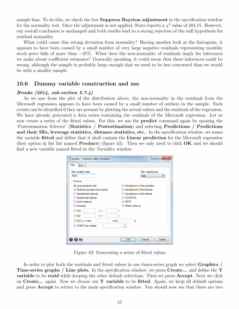
sample bias. To do this, we check the box Suppress Royston adjustment in the specification windowfor the normality test. Once the adjustment is not applied, Stata reports a χ2 value of 204.15. However,our overall conclusion is unchanged and both results lead to a strong rejection of the null hypothesis forresidual normality.

What could cause this strong deviation from normality? Having another look at the histogram, itappears to have been caused by a small number of very large negative residuals representing monthlystock price falls of more than −25%. What does the non-normality of residuals imply for inferenceswe make about coefficient estimates? Generally speaking, it could mean that these inferences could bewrong, although the sample is probably large enough that we need to be less concerned than we wouldbe with a smaller sample.

10.6 Dummy variable construction and use

Brooks (2014, sub-section 5.7.4)As we saw from the plot of the distribution above, the non-normality in the residuals from the

Microsoft regression appears to have been caused by a small number of outliers in the sample. Suchevents can be identified if they are present by plotting the actual values and the residuals of the regression.We have already generated a data series containing the residuals of the Microsoft regression. Let usnow create a series of the fitted values. For this, we use the predict command again by opening the‘Postestimation Selector’ (Statistics / Postestimation) and selecting Predictions / Predictionsand their SEs, leverage statistics, distance statistics, etc.. In the specification window, we namethe variable fitted and define that it shall contain the Linear prediction for the Microsoft regression(first option in list list named Produce) (figure 43). Then we only need to click OK and we shouldfind a new variable named fitted in the Variables window.

Figure 43: Generating a series of fitted values

In order to plot both the residuals and fitted values in one times-series graph we select Graphics /Time-series graphs / Line plots. In the specification window, we press Create... and define the Yvariable to be resid while keeping the other default selections. Then we press Accept. Next we clickon Create... again. Now we choose our Y variable to be fitted. Again, we keep all default optionsand press Accept to return to the main specification window. You should now see that there are two

57

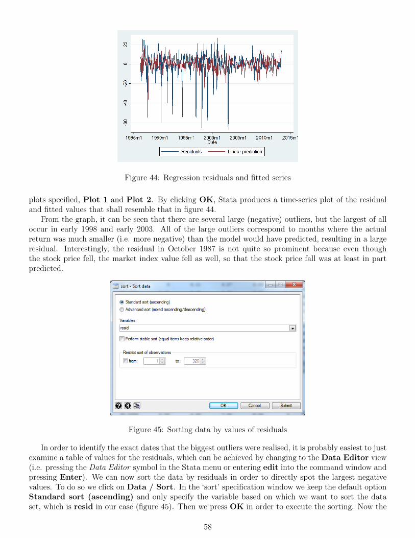
Figure 44: Regression residuals and fitted series

plots specified, Plot 1 and Plot 2. By clicking OK, Stata produces a time-series plot of the residualand fitted values that shall resemble that in figure 44.

From the graph, it can be seen that there are several large (negative) outliers, but the largest of alloccur in early 1998 and early 2003. All of the large outliers correspond to months where the actualreturn was much smaller (i.e. more negative) than the model would have predicted, resulting in a largeresidual. Interestingly, the residual in October 1987 is not quite so prominent because even thoughthe stock price fell, the market index value fell as well, so that the stock price fall was at least in partpredicted.

Figure 45: Sorting data by values of residuals

In order to identify the exact dates that the biggest outliers were realised, it is probably easiest to justexamine a table of values for the residuals, which can be achieved by changing to the Data Editor view(i.e. pressing the Data Editor symbol in the Stata menu or entering edit into the command window andpressing Enter). We can now sort the data by residuals in order to directly spot the largest negativevalues. To do so we click on Data / Sort. In the ‘sort’ specification window we keep the default optionStandard sort (ascending) and only specify the variable based on which we want to sort the dataset, which is resid in our case (figure 45). Then we press OK in order to execute the sorting. Now the

58

dataset should be sorted by ‘resid’, starting with the lowest values and ending with the highest valuesfor ‘resid’.

If we do this, it is evident that the two most extreme residuals (with values to the nearest integer)were in February 1998 (−65.59529) and February 2003 (−66.98543).

One way of removing the (distorting) effect of big outliers in the data is by using dummy variables.It would be tempting, but incorrect, to construct one dummy variable that takes the value 1 for bothFeb 98 and Feb 03, but this would not have the desired effect of setting both residuals to zero. Instead,to remove two outliers requires us to construct two separate dummy variables. In order to create theFeb 98 dummy first, we generate a series called ‘FEB98DUM’ that will initially contain only zeros. Todo this we return to the main Stata screen and click on Data / Create or change data / Createnew variable. In the variable specification window, we change the Variable type to byte (as dummyvariables are binary variables) and define Variable name: FEB98DUM (figure 46).

Figure 46: Creating a Dummy variable for Outliers I

Now we need to specify the content of the variable which we do in the following way: In the Specifya value or an expression box we type in:1 if Date==tm(1998m2)

which means that the new variable takes the value of one if the Date is equal to 1998m2. Note thatthe function tm() is used to allow us to type the Date as a human readable date instead of the codedStata value.42 All other values (except February 1998) are missing values. To change these values tozero we can click on Data / Create or change data / Change contents of variable and in thenew window we select the variable FEB98DUM and specify the New content to be0 if Date!=tm(1998m2)where ‘Date!=tm(1998m2)’ means if the Date is not equal to February 1998 (figure 47).

We can check whether the dummy is correctly specified by visually inspecting the FEB98DUMseries in the Data Editor. There should only be one single observation for which the dummy takes thevalue of one, which is February 1998, whereas it should be zero for all other dates.

We repeat the process above to create another dummy variable called ‘FEB03DUM’ that takesthe value 1 in February 2003 and zero elsewhere.

42Alternatively, you could have simply used the following commands to generate the series: generate byteFEB98DUM = 1 if Date==tm(1998m2) and replace FEB98DUM = 0 if Date!=tm(1998m2).

59

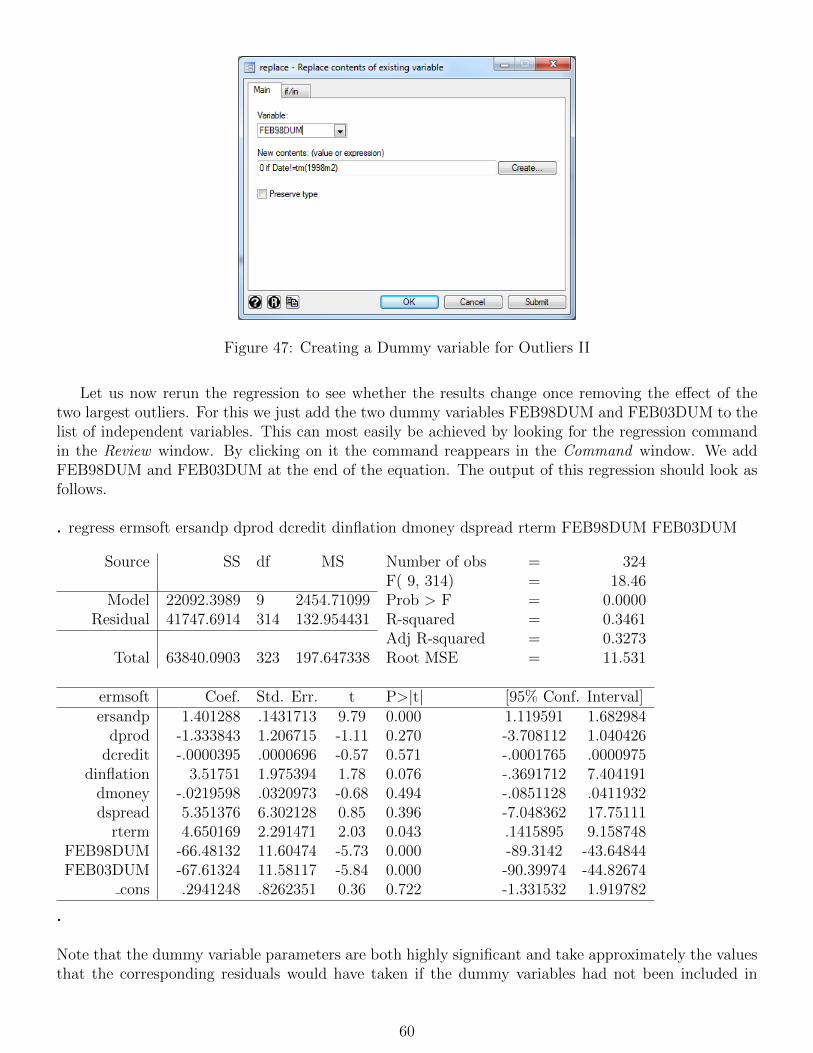
Figure 47: Creating a Dummy variable for Outliers II

Let us now rerun the regression to see whether the results change once removing the effect of thetwo largest outliers. For this we just add the two dummy variables FEB98DUM and FEB03DUM to thelist of independent variables. This can most easily be achieved by looking for the regression commandin the Review window. By clicking on it the command reappears in the Command window. We addFEB98DUM and FEB03DUM at the end of the equation. The output of this regression should look asfollows.

. regress ermsoft ersandp dprod dcredit dinflation dmoney dspread rterm FEB98DUM FEB03DUM

Source SS df MS Number of obs = 324F( 9, 314) = 18.46

Model 22092.3989 9 2454.71099 Prob > F = 0.0000Residual 41747.6914 314 132.954431 R-squared = 0.3461

Adj R-squared = 0.3273Total 63840.0903 323 197.647338 Root MSE = 11.531

ermsoft Coef. Std. Err. t P>|t| [95% Conf. Interval]ersandp 1.401288 .1431713 9.79 0.000 1.119591 1.682984

dprod -1.333843 1.206715 -1.11 0.270 -3.708112 1.040426dcredit -.0000395 .0000696 -0.57 0.571 -.0001765 .0000975

dinflation 3.51751 1.975394 1.78 0.076 -.3691712 7.404191dmoney -.0219598 .0320973 -0.68 0.494 -.0851128 .0411932dspread 5.351376 6.302128 0.85 0.396 -7.048362 17.75111

rterm 4.650169 2.291471 2.03 0.043 .1415895 9.158748FEB98DUM -66.48132 11.60474 -5.73 0.000 -89.3142 -43.64844FEB03DUM -67.61324 11.58117 -5.84 0.000 -90.39974 -44.82674

cons .2941248 .8262351 0.36 0.722 -1.331532 1.919782

.

Note that the dummy variable parameters are both highly significant and take approximately the valuesthat the corresponding residuals would have taken if the dummy variables had not been included in

60

the model.43 By comparing the results with those of the regression above that excluded the dummyvariables, it can be seen that the coefficient estimates on the remaining variables change quite a bit in thisinstance and the significances improve considerably. The term structure parameter is now significantat the 5% level and the unexpected inflation parameter is now significant at the 10% level. The R2

value has risen from 0.21 to 0.35 because of the perfect fit of the dummy variables to those two extremeoutlying observations.

Finally, we can re-examine the normality test results of the residuals based on this new modelspecification. First we have to create the new residual series by opening the ‘predict’ specification window(Statistics / Postestimation / Predictions / Predictions and their SEs, leverage statistics,distance statistics, etc.). We name the new residual series resid new and select the second Produceoption Residuals (equation-level scores). Then we re-run the Skewness and Kurtosis test (sktest)on this new series of residuals using Statistics / Summaries, tables, and tests / Distributionalplots and tests / Skewness and kurtosis normality test. Note that we can test both versions,with and without the Royston adjustment for small sample bias.

We see that the residuals are still a long way from following a normal distribution, and that thenull hypothesis of normality is still strongly rejected, probably because there are still several very largeoutliers. While it would be possible to continue to generate dummy variables, there is a limit to theextent to which it would be desirable to do so. With this particular regression, we are unlikely to beable to achieve a residual distribution that is close to normality without using an excessive number ofdummy variables. As a rule of thumb, in a monthly sample with 324 observations, it is reasonable toinclude, perhaps, two or three dummy variables for outliers, but more would probably be excessive.

10.7 Multicollinearity

Brooks (2014, section 5.8)Let us assume that we would like to test for multicollinearity issues in the Microsoft regression

(‘macro.dta’ workfile). To generate a correlation matrix in Stata, we click on Statistics / Summaries,tables, and test / Summary and descriptive statistics / Correlations and covariances. Inthe Variables dialogue box we enter the list of regressors (not including the regressand or the S&P500returns), as in figure 48.

After clicking OK, the following correlation matrix shall appear in the Output window.

. correlate dprod dcredit dinflation dmoney dspread rterm

(obs=324)dprod dcredit dinfla∼ n dmoney dspread rterm

dprod 1.0000dcredit 0.1411 1.0000

dinflation -0.1243 0.0452 1.0000dmoney -0.1301 -0.0117 -0.0980 1.0000dspread -0.0556 0.0153 -0.2248 0.2136 1.0000

rterm -0.0024 0.0097 -0.0542 -0.0862 0.0016 1.0000

.

Do the results indicate any significant correlations between the independent variables? In this par-

43Note the inexact correspondence between the values of the residuals and the values of the dummy variable parametersbecause two dummies are being used together; had we included only one dummy, the value of the dummy variablecoefficient and that which the residual would have taken would be identical.

61

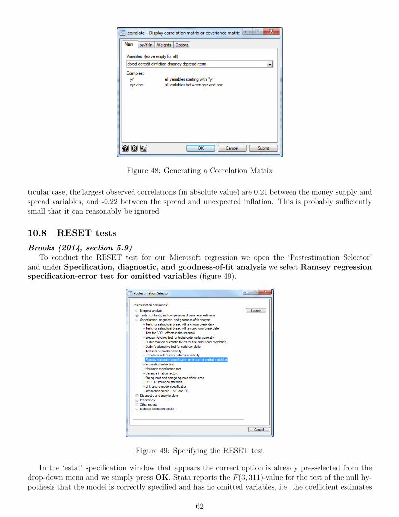
Figure 48: Generating a Correlation Matrix

ticular case, the largest observed correlations (in absolute value) are 0.21 between the money supply andspread variables, and -0.22 between the spread and unexpected inflation. This is probably sufficientlysmall that it can reasonably be ignored.

10.8 RESET tests

Brooks (2014, section 5.9)To conduct the RESET test for our Microsoft regression we open the ‘Postestimation Selector’

and under Specification, diagnostic, and goodness-of-fit analysis we select Ramsey regressionspecification-error test for omitted variables (figure 49).

Figure 49: Specifying the RESET test

In the ‘estat’ specification window that appears the correct option is already pre-selected from thedrop-down menu and we simply press OK. Stata reports the F (3, 311)-value for the test of the null hy-pothesis that the model is correctly specified and has no omitted variables, i.e. the coefficient estimates

62

on the powers of the higher order terms of the fitted values are zero:

. estat ovtest

Ramsey RESET test using powers of the fitted values of ermsoftHo: model has no omitted variables

F(3, 311) = 1.01Prob > F = 0.3897

.

Based on the F -statistic having 3 degrees of freedom we can assume that Stata included three higherorder terms of the fitted values in auxiliary regressions. With an F -value of 1.01 and a correspondingp-value of 0.3897, the RESET test results imply that we cannot reject the null hypothesis that themodel has no omitted variables. In other words, we do not find strong evidence that the chosen linearfunctional form of the model is incorrect.

10.9 Stability tests

Brooks (2014, section 5.12)There are two types of stability tests that we want to apply: the Chow (analysis of variance) test and

the predictive failure test. To access the Chow test, we open the ‘Postestimation Selector’ (Statistics/ Postestimation) and select Specification, diagnostic, and goodness-of-fit analysis. Note thatit is not possible to conduct a Chow test or a parameter stability test when there are outlier dummyvariables in the regression. THus, we have to ensure that the last estimation that we run is the Microsoftregression omitting the FEB98DUM and FEB03DUM dummies from the list of independent variables.44

This occurs because when the sample is split into two parts, the dummy variable for one of the partswill have values of zero for all observations, which would thus cause perfect multicollinearity with thecolumn of ones that is used for the constant term. Looking at the ‘Postestimation Selector’, we seethat there are two tests for structural breaks, one which tests for structural breaks with a known breakdate and one test for structural breaks when the break date is unknown. Let us first run Tests forstructural berak with a known break date by selecting the corresponding option (figure 50, leftpanel). In the specification window that appears, we are now asked to specify the ‘Hypothesized breakdates’ (figure 50, right panel).

Let us assume that we want to test whether a breakpoint occurred in January 1996, which is roughlyin the middle of the sample period. Thus, we specify Hypothesized break dates: tm(1996m1).Note that the ‘tm()’ is used to tell Stata that the term in the brackets is formatted as a monthly datevariable. In the box titled Break variables we could select specific variables of the model to be includedin the test. By default, all coefficients are tested. As we do not have any priors as to which variablesmight be subject to a structural break and which are not, we leave this box empty, and simply pressOK to generate the following test statistics.

44The corresponding command for this regression is: regress ermsoft ersandp dprod dcredit dinflation dmoney dspreadrterm.

63

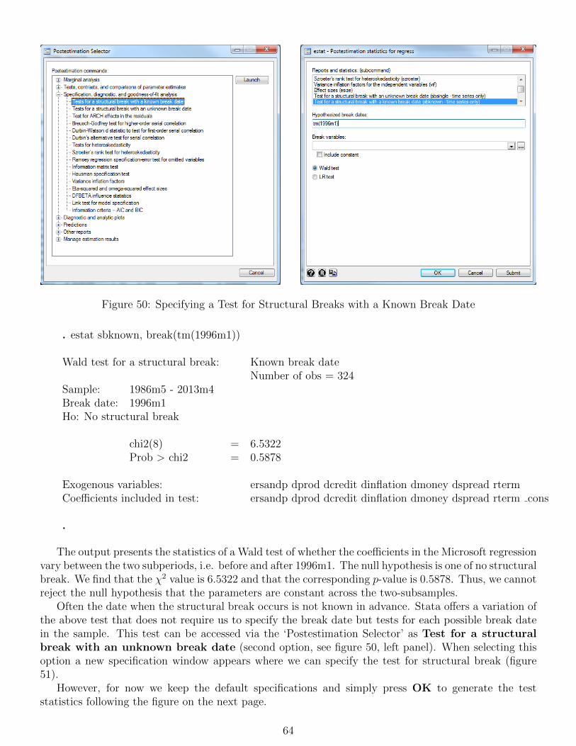
Figure 50: Specifying a Test for Structural Breaks with a Known Break Date

. estat sbknown, break(tm(1996m1))

Wald test for a structural break: Known break dateNumber of obs = 324

Sample: 1986m5 - 2013m4Break date: 1996m1Ho: No structural break

chi2(8) = 6.5322Prob > chi2 = 0.5878

Exogenous variables: ersandp dprod dcredit dinflation dmoney dspread rtermCoefficients included in test: ersandp dprod dcredit dinflation dmoney dspread rterm cons

.

The output presents the statistics of a Wald test of whether the coefficients in the Microsoft regressionvary between the two subperiods, i.e. before and after 1996m1. The null hypothesis is one of no structuralbreak. We find that the χ2 value is 6.5322 and that the corresponding p-value is 0.5878. Thus, we cannotreject the null hypothesis that the parameters are constant across the two-subsamples.

Often the date when the structural break occurs is not known in advance. Stata offers a variation ofthe above test that does not require us to specify the break date but tests for each possible break datein the sample. This test can be accessed via the ‘Postestimation Selector’ as Test for a structuralbreak with an unknown break date (second option, see figure 50, left panel). When selecting thisoption a new specification window appears where we can specify the test for structural break (figure51).

However, for now we keep the default specifications and simply press OK to generate the teststatistics following the figure on the next page.

64

Figure 51: Specifying a Test for Structural Breaks with an Unknown Break Date

. estat sbsingle

1 —-+—- 2 —-+—- 3 —-+—– 4 —-+—- 5.................................................. 50.................................................. 100.................................................. 150.................................................. 200..........................

Test for a structural break: Unknown break dateNumber of obs = 324

Full sample: 1986m5 - 2013m4Trimmed sample: 1990m6 - 2009m4Estimated break date: 1990m8Ho: No structural breakTest Statistic p-value

swald 12.0709 0.7645

Exogenous variables: ersandp dprod dcredit dinflation dmoney dspread rtermCoefficients included in test: ersandp dprod dcredit dinflation dmoney dspread rterm cons

.

Again the null hypothesis is one of no structural breaks. The test statistic and the corresponding p-valuesuggest that we cannot reject the null hypothesis that the coefficients are stable over time confirmingthat our model does not have a structural break for any possible break date in the sample.

Another way of testing whether the parameters are stable with respect to any break dates is to useone of the tests based on recursive estimation. Unfortunately, there is no built-in function in Stata thatautomatically produces plots of the recursive coefficient estimates together with standard error bands.In order to visually investigate the parameter stability, we have to run recursive estimations and savethe parameter estimates (in a new file). Then we can plot these data series.

To do so we first select Statistics / Time series / Rolling-window and recursive estimation.

65

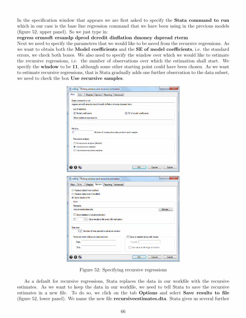
In the specification window that appears we are first asked to specify the Stata command to runwhich in our case is the base line regression command that we have been using in the previous models(figure 52, upper panel). So we just type in:regress ermsoft ersandp dprod dcredit dinflation dmoney dspread rtermNext we need to specify the parameters that we would like to be saved from the recursive regressions. Aswe want to obtain both the Model coefficients and the SE of model coefficients, i.e. the standarderrors, we check both boxes. We also need to specify the window over which we would like to estimatethe recursive regressions, i.e. the number of observations over which the estimation shall start. Wespecify the window to be 11, although some other starting point could have been chosen. As we wantto estimate recursive regressions, that is Stata gradually adds one further observation to the data subset,we need to check the box Use recursive samples.

Figure 52: Specifying recursive regressions

As a default for recursive regressions, Stata replaces the data in our workfile with the recursiveestimates. As we want to keep the data in our workfile, we need to tell Stata to save the recursiveestimates in a new file. To do so, we click on the tab Options and select Save results to file(figure 52, lower panel). We name the new file recursiveestimates.dta. Stata gives us several further

66

options, e.g. to specify the steps of the recursive estimations or the start and end date; but we leave thespecifications as they are and press OK to generate the recursive estimates.

As you can see from the Output window, Stata does not report the regression results for each of the316 recursive estimations, but produces a ‘.’ for each regression. To access the recursive estimates, weneed to open the new workfile ‘recursiveestimates.dta’ that should be stored in the same folder as theoriginal workfile ‘macro.dta’. You can open it by double-clicking on the file. The ‘recursiveestimates.dta’workfile contains several data series: start and end contain the start date and the end date overwhich the respective parameters have been estimated; b ersandp, for example, contains the recursivecoefficient estimates for the excess S&P500 returns, while se ersandp contains the correspondingstandard errors of the coefficient estimate.

In order to visually investigate the parameter stability over the recursive estimations, it is best togenerate a time-series plot of the recursive estimates. Assume we would like to generate such a plotfor the recursive estimates of ersandp. We would like to plot the actual recursive coefficients togetherwith standard error bands. So first, we need to generate data series for the standard error bands. Wedecide to generate two series: one for a deviation of 2 standard errors above the coefficient estimate( b ersandp plus2SE) and one for a deviation of 2 standard errors below the coefficient estimate( b ersandp minus2SE). To do so, we use the following two commands to generate the two series:generate b ersandp plus2SE = b ersandp + 2* se ersandpgenerate b ersandp minus2SE = b ersandp - 2* se ersandp

Once we have generated the new variables, we can plot them together with the actual recursivecoefficients of ‘ersandp’. We click on Graphics / Time-series graphs / Line plots. In the graphspecification window we click on Create... to specify the first data series which is the recursive coefficientestimates for ‘ersandp’ ( b ersandp). In the dialogue box named Y variable we type in ( b ersandp)and click on Line properties to format this particular data series (figures 53, top two panels).

We change the Color to Blue and the Pattern to Solid and press Accept. Then we press Acceptagain to return to the main graph specification window. We now click on Create... to specify the nextseries to be included in the graph which is the positive 2 standard error series ( b ersandp plus2SE).We select this variable from the drop-down menu and click on Line properties. For this data se-ries, we select the Color to be Red and the Pattern to be Dash and click Accept twice to re-turn to the main specification window. We generate Plot 3 of the negative 2 standard error series( b ersandp minus2SE) in a similar way as the previous series, again selecting Color: Red andPattern: Dash. Finally, we need to specify the time variable by clicking on Time settings... in themain specification window. In the auxiliary window that appears we define the Time variable to beend and click OK (figure 53, bottom panel). Now that we have specified all graph characteristics wesimply need to press OK to generate the graph.

What do we observe from the graph (figure 54)? The coefficients of the first couple of sub-samplesseem to be relatively unstable with large standard error bands while they seem to stabilise after a shortperiod of time and only show small standard error bands. This pattern is to be expected as it takessome time for the coefficients to stabilise since the first few sets are estimated using very small samples.Given this, the parameter estimates are remarkably stable. We can repeat this process for the recursiveestimates of the other variables to see whether they show similar stability over time. Unfortunately,there is no built-in Stata function for the CUSUM and CUSUMSQ stability tests.

67

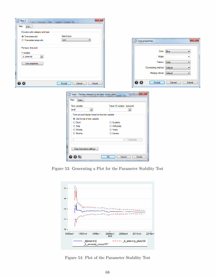
Figure 53: Generating a Plot for the Parameter Stability Test

Figure 54: Plot of the Parameter Stability Test

68

11 Constructing ARMA models

Brooks (2014, sections 6.7 & 6.8)

Getting started

This example uses the monthly UK house price series which was already incorporated in a Stata workfilein section 2 (‘ukhp.dta’). So first we re-load the workfile into Stata. There are a total of 268 monthlyobservations running from February 1991 (recall that the January observation was ‘lost’ in constructingthe lagged value) to May 2013 for the percentage change in house price series. The objective of thisexercise is to build an ARMA model for the house price changes. Recall that there are three stagesinvolved: identification, estimation and diagnostic checking. The first stage is carried out by looking atthe autocorrelation and partial autocorrelation coefficients to identify any structure in the data.

Estimating autocorrelation coefficients

To generate a table of autocorrelations, partial correlations and related test statistics we click on Statis-tics / Time series / Graphs and select the option Autocorrelations & partial autocorrelations.In the specification window that appears we select dhp as the variable for which we want to generate theabove statistics and specify that we want to use 12 lags as the specified number of autocorrelations(figure 55).

Figure 55: Generating a Correlogram

By clicking OK, the correlogram appears in the Stata Output window, as given below.45

45Note that the graphs for the AC and PAC values are very small. You can generate individual graphs for the AC andPAC including confidence bands by selecting Statistics / Time series / Graphs / Correlogram (ac) and Statistics/ Time series / Graphs / Partial correlogram (pac), respectively.

69

. corrgram dhp, lags(12)

-1 0 1 -1 0 1LAG AC PAC Q Prob>Q [Autocorrelation] [Partial Autocor]1 0.3561 0.3569 34.36 0.0000 – –2 0.4322 0.3499 85.175 0.0000 — –3 0.2405 0.0183 100.96 0.0000 -4 0.2003 -0.0145 111.96 0.0000 -5 0.1388 0.0044 117.26 0.0000 -6 0.1384 0.0492 122.55 0.0000 -7 0.0742 -0.0222 124.07 0.00008 0.1168 0.0528 127.87 0.00009 0.1756 0.1471 136.49 0.0000 - -10 0.1414 0.0259 142.09 0.0000 -11 0.2474 0.1266 159.32 0.0000 - -12 0.2949 0.1851 183.9 0.0000 – -

.

It is clearly evident that the series is quite persistent given that it is already in percentage changeform. The autocorrelation function dies away rather slowly. Only the first two partial autocorrelationcoefficients appear strongly significant. The numerical values of the autocorrelation and partial auto-correlation coefficients at lags 1–12 are given in the second and third columns of the output, with thelag length given in the first column.

Remember that as a rule of thumb, a given autocorrelation coefficient is classed as significant ifit is outside a ±1.96× 1/(T )1/2 band, where T is the number of observations. In this case, it wouldimply that a correlation coefficient is classed as significant if it is bigger than approximately 0.11 orsmaller than −0.11. The band is of course wider when the sampling frequency is monthly, as it ishere, rather than daily where there would be more observations. It can be deduced that the first sixautocorrelation coefficients (then eight through 12) and the first two partial autocorrelation coefficients(then nine, 11 and 12) are significant under this rule. Since the first acf coefficient is highly significant,the joint test statistic presented in column 4 rejects the null hypothesis of no autocorrelation at the1% level for all numbers of lags considered. It could be concluded that a mixed ARMA process mightbe appropriate, although it is hard to precisely determine the appropriate order given these results. Inorder to investigate this issue further, information criteria are now employed.

Using information criteria to decide on model orders

An important point to note is that books and statistical packages often differ in their construction of thetest statistic. For example, the formulae given in Brooks (2014) for Akaike’s and Schwarz’s InformationCriteria are

AIC = ln(σ2) +2k

T(1)

SBIC = ln(σ2) +k

T(ln T ) (2)

where, σ2 is the estimator of the variance of regressions disturbances ut, k is the number of parametersand T is the sample size. When using the criterion based on the estimated standard errors, the modelwith the lowest value of AIC and SBIC should be chosen. On the other hand, Stata uses a formulation of

70

the test statistic based on the log-likelihood function value derived from maximum likelihood estimation.The corresponding Stata formulae are

AIC` = −2 ∗ ln(likelihood) + 2k (3)

SBIC` = −2 ∗ ln(likelihood) + ln(T ) ∗ k (4)

Unfortunately, this modification is not benign, since it affects the relative strength of the penaltyterm compared with the error variance, sometimes leading different packages to select different modelorders for the same data and criterion!

Figure 56: Specifying an ARMA(1,1) model

Suppose that it is thought that ARMA models from order (0,0) to (5,5) are plausible for the houseprice changes. This would entail considering 36 models (ARMA(0,0), ARMA(1,0), ARMA(2,0), . . . ARMA(5,5)),i.e. up to 5 lags in both the autoregressive and moving average terms.

In Stata, this can be done by by separately estimating each of the models and noting down thevalue of the information criteria in each case. We can do this in the following way. On the Stata mainmenu, we click on Statistics / Time series and select ARIMA and ARMAX models. In thespecification window that appears we select Dependent variable: dhp and leave the dialogue box forthe independent variables empty as we only want to include autoregressive and moving-average terms butno other explanatory variables. We are then asked to specify the ARMA model. There are three boxes inwhich we can type in the number of either the autoregressive order (p), the intergrated (difference) order(d) or the moving-average order (q). As we want to start with estimating an ARMA(1,1) model, i.e.a model of autoregressive order 1 and moving-average order 1, we specify this in the respectiveboxes (figure 56).

We click OK and Stata generates the following estimation output.

71

. arima dhp, arima(1,0,1)

(setting optimization to BHHH)Iteration 0: log likelihood = -402.99577Iteration 1: log likelihood = -398.44455Iteration 2: log likelihood = -398.17002Iteration 3: log likelihood = -398.14678Iteration 4: log likelihood = -398.1451(switching optimization to BFGS)Iteration 5: log likelihood = -398.14496Iteration 6: log likelihood = -398.14495

ARIMA regression

Sample: 1991m2 - 2013m5 Number of obs = 268Wald chi2(2) = 321.20

Log likelihood = -398.1449 Prob > chi2 = 0.0000

OPGdhp Coef. Std. Err. z P>|z| [95% Conf. Interval]

dhpcons .4442364 .1778922 2.50 0.013 .095574 .7928988

ARIMAar

L1. .8364163 .0592257 14.12 0.000 .7203361 .9524966

maL1. -.560846 .0949258 -5.91 0.000 -.7468972 -.3747949

/sigma 1.06831 .0424821 25.15 0.000 .9850461 1.151573

Note: The test of the variance against zero is one sided, and the two-sided confidence interval is trun-cated at zero..

In theory, the output would be discussed in a similar way to the simple linear regression modeldiscussed in section 3. However, in reality it is very difficult to interpret the parameter estimates in thesense of, for example, saying ‘a 1 unit increase in x leads to a β unit increase in y’. In part because theconstruction of ARMA models is not based on any economic or financial theory, it is often best not toeven try to interpret the individual parameter estimates, but rather to examine the plausibility of themodel as a whole, and to determine whether it describes the data well and produces accurate forecasts(if this is the objective of the exercise, which it often is). Note also that the header of the Stata outputfor ARMA models states the number of iterations that have been used in the model estimation process.This shows that, in fact, an iterative numerical optimisation procedure has been employed to estimatethe coefficients.

In order to generate the information criteria corresponding to the ARMA(1,1) model we open the‘Postestimation Selector’ (Statistics / Postestimation) and select Specification, diagnostic, andgoodness-of-fit analysis (figure 57, left panel). In the specification window, the correct subcommandinformation criteria (ic) is already pre-selected (figure 57, right panel). We can specify the numberof observations for calculating the SBIC (Schwartz criterion), though we keep the default option which

72

is all 268 observations.

Figure 57: Generating Information Criteria for the ARMA(1,1) model

By clicking OK the following test statistics are generated.

. estat ic

Model Obs ll(null) ll(model) df AIC BIC

. 268 . -398.1449 4 804.2899 818.6538

Note: N=Obs used in calculating BIC; see [R] BIC note

.

We see that the AIC has a value of 804.29 and the BIC a value of 818.65. However, by themselvesthese two statistics are relatively meaningless for our decision as to which ARMA model to choose.Instead, we need to generate these statistics for the competing ARMA models and then select the modelwith the lowest information criterion.

To check that the process implied by the model is stationary and invertible it is useful to look atthe inverses of the AR and MA roots of the characteristic equation. If the inverse roots of the ARpolynomial all lie inside the unit circle, the process is stationary, invertible, and has an infinite-ordermoving-average (MA) representation. We can test this by selecting Diagnostic and analytic plots /Check stability condition of estimates in the ‘Postestimation Selector’ (figure 58, upper left panel).In the specification window that appears we tick the box Label eigenvalues with the distance fromthe unit circle and click OK (figure 58, upper right panel). From the test output we see that theinverted roots for both the AR and MA parts lie inside the unit circle and have a distance from thecircle of 0.164 and 0.439, respecively (figure 58, bottom panel). Thus the conditions of stationarity andinvertibility, respectively, are met.

73

Figure 58: Testing the Stability Condition for the ARMA(1,1) estimates

74

Figure 59: Specifying an ARMA(5,5) model

Repeating these steps for the other ARMA models would give all of the required values for theinformation criteria. To give just one more example, in the case of an ARMA(5,5), the following wouldbe typed in the ARMA specification window (figure 59).46

Again, we need to generate the information critera by selecting Specification, diagnostic, andgoodness-of-fit analysis.

The following table reports values of the information criteria for all the competing ARMA models,calculated via Stata.

Information criteria for ARMA models of thepercentage changes in UK house prices

AICp/q 0 1 2 3 4 50 861.4978 842.7697 806.4366 803.7957 802.0392 801.49061 827.1883 804.2899 797.5436 796.1649 797.3497 801.30952 794.2106 796.1276 798.0601 796.8032 798.288 798.29673 796.1206 795.4963 800.0436 798.5315 797.9832 789.85794 798.0641 797.3843 794.4796 765.7066 799.9824 789.74515 800.0589 798.4508 796.4047 795.1458 796.719 764.9448

SBICp/q 0 1 2 3 4 50 868.6797 853.5427 820.8005 821.7506 823.5851 826.62751 837.9613 818.6538 815.4985 817.7108 822.4866 830.03742 808.5745 814.0825 819.606 821.9401 827.0159 830.61553 814.0756 817.0423 825.1805 827.2593 830.3021 825.76784 819.6101 822.5212 823.2075 794.4345 835.8923 829.2465 825.1958 827.1787 828.7236 831.0557 836.2199 804.4457

So which model actually minimises the two information criteria? In this case, the criteria choose differentmodels: AIC selects an ARMA(5,5), while SBIC selects the smaller ARMA(4,3) model. These chosenmodels are highlighted in bold in the table. It will always be the case that SBIC selects a model that

46For more information on how to specify ARMA and ARIMA models in Stata, refer to the respective entry in theStata manual.

75

is at least as small (i.e. with fewer or the same number of parameters) as AIC, because the formercriterion has a stricter penalty term. This means that SBIC penalises the incorporation of additionalterms more heavily. Many different models provide almost identical values of the information criteria,suggesting that the chosen models do not provide particularly sharp characterisations of the data andthat a number of other specifications would fit the data almost as well.

76

12 Forecasting using ARMA models

Brooks (2014, section 6.12)Suppose that a AR(2) model selected for the house price percentage changes series were estimated us-

ing observations February 1991–December 2010, leaving 29 remaining observations to construct forecastsfor and to test forecast accuracy (for the period January 2011–May 2013).

Figure 60: Specifying an ARMA(2,0) model for the Sub-period 1991m2 - 2010m12

Let us first estimate the ARMA(2,0) model for the time period 1991m2 - 2010m12. The specificationwindow for estimating this model shall resemble figure 60, upper panel. We select 2 as the Autoregres-sive order (p) and leave the other model parts as zero. As we only want to estimate the model over asub-period of the data, we next select the tab by/if/in (figure 60, bottom panel). In the dialogue boxIf: (expression) we type in Month<=tm(2010m12). Next, we click Ok and the following regressionoutput should appear in the Output window.

77

. arima dhp if Month<=tm(2012m12), arima(2,0,0)

(setting optimization to BHHH)Iteration 0: log likelihood = -356.02571Iteration 1: log likelihood = -356.01987Iteration 2: log likelihood = -356.01932Iteration 3: log likelihood = -356.01927Iteration 4: log likelihood = -356.01926

ARIMA regression

1991m2 - 2010m12 Number of obs = 239Wald chi2(2) = 73.56

Log likelihood = -356.0193 Prob > chi2 = 0.0000

OPGdhp Coef. Std. Err. z P>|z| [95% Conf. Interval]

dhpcons .4626106 .170433 2.71 0.007 .1285681 .7966532

ARIMAar

L1. .2253595 .053378 4.22 0.000 .1207406 .3299783L2. .3623799 .0514643 7.04 0.000 .2615118 .463248

/sigma 1.072291 .0464221 23.10 0.000 .9813056 1.163277

Note: The test of the variance against zero is one sided, and the two-sided confidence interval is trun-cated at zero..

Now that we have fit the model we can produce the forcasts for the period 2011m1 to 2013m5.There are two methods available in Stata for constructing forecasts: dynamic and static. The optionDynamic calculates multi-step forecasts starting from the first period in the forecast sample. Staticforecasts imply a sequence of one-step-ahead forecasts, rolling the sample forwards one observation aftereach forecast.

We start with generating static forecasts. These forecasts can be generated by opening the ‘Postes-timation Selector’ and choosing Predictions / Means from the differenced or undifferencedseries, mean squared errors, residuals, etc. (figure 61).

In the ‘predict’ specification window, we are first asked to name the variable that shall contain thepredictions (figure 62, upper left panel). We choose to name the static forecasts dhpf stat. As we wantto create predicted/fitted values, we keep the default option under Produce which is Values for meanequation. If we change to the Options tab now, the window should resemble that in figure 62, upperright panel. We see that the option One-step prediction is selected as default, so we do not need tomake any changes at this stage. We simply click OK and we should find the new series appearing inour Variables window.

We create the dynamic forecasts in a similar way. First we open the ‘predict’ specification windowagain, and name the series that shall contain the dynamic forecasts dhpf dyn. Then we change to theOptions tab. Here we select the option Switch to dynamic predictions at time: and we specifythe time as tm(2011m1), i.e. the start of the forecast period. By clicking OK we generate the seriesof dynamic forecasts (figure 62, bottom panel).

78

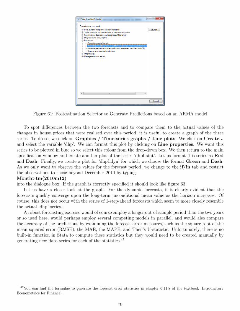
Figure 61: Postestimation Selector to Generate Predictions based on an ARMA model

To spot differences between the two forecasts and to compare them to the actual values of thechanges in house prices that were realised over this period, it is useful to create a graph of the threeseries. To do so, we click on Graphics / Time-series graphs / Line plots. We click on Create...and select the variable ‘dhp’. We can format this plot by clicking on Line properties. We want thisseries to be plotted in blue so we select this colour from the drop-down box. We then return to the mainspecification window and create another plot of the series ‘dhpf stat’. Let us format this series as Redand Dash. Finally, we create a plot for ‘dhpf dyn’ for which we choose the format Green and Dash.As we only want to observe the values for the forecast period, we change to the if/in tab and restrictthe observations to those beyond December 2010 by typingMonth>tm(2010m12)into the dialogue box. If the graph is correctly specified it should look like figure 63.

Let us have a closer look at the graph. For the dynamic forecasts, it is clearly evident that theforecasts quickly converge upon the long-term unconditional mean value as the horizon increases. Ofcourse, this does not occur with the series of 1-step-ahead forecasts which seem to more closely resemblethe actual ‘dhp’ series.

A robust forecasting exercise would of course employ a longer out-of-sample period than the two yearsor so used here, would perhaps employ several competing models in parallel, and would also comparethe accuracy of the predictions by examining the forecast error measures, such as the square root of themean squared error (RMSE), the MAE, the MAPE, and Theil’s U-statistic. Unfortunately, there is nobuilt-in function in Stata to compute these statistics but they would need to be created manually bygenerating new data series for each of the statistics.47

47You can find the formulae to generate the forecast error statistics in chapter 6.11.8 of the textbook ‘IntroductoryEconometrics for Finance’.

79

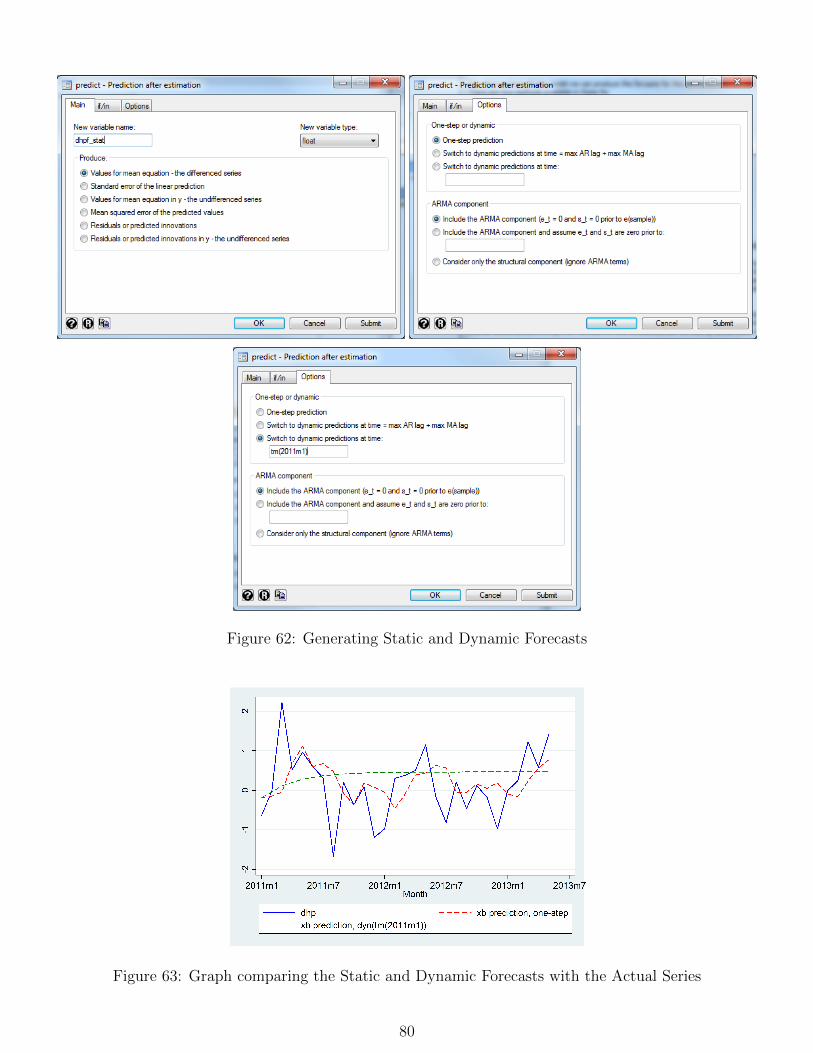
Figure 62: Generating Static and Dynamic Forecasts

Figure 63: Graph comparing the Static and Dynamic Forecasts with the Actual Series

80

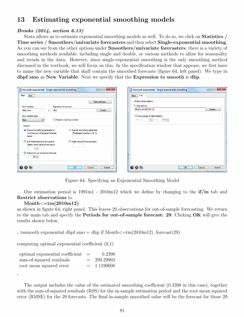
13 Estimating exponential smoothing models

Brooks (2014, section 6.13)Stata allows as to estimate exponential smoothing models as well. To do so, we click on Statistics /

Time series / Smoothers/univariate forecasters and then select Single-exponential smoothing.As you can see from the other options under Smoothers/univariate forecasters, there is a variety ofsmoothing methods available, including single and double, or various methods to allow for seasonalityand trends in the data. However, since single-exponential smoothing is the only smoothing methoddiscussed in the textbook, we will focus on this. In the specification window that appears, we first haveto name the new variable that shall contain the smoothed forecasts (figure 64, left panel). We type indhpf smo as New Variable. Next we specify that the Expression to smooth is dhp.

Figure 64: Specifying an Exponential Smoothing Model

Our estimation period is 1991m1 - 2010m12 which we define by changing to the if/in tab andRestrict observations to

Month<=tm(2010m12)as shown in figure 64, right panel. This leaves 29 observations for out-of-sample forecasting. We returnto the main tab and specify the Periods for out-of-sample forecast: 29. Clicking OK will give theresults shown below.

. tssmooth exponential dhpf smo = dhp if Month<=tm(2010m12), forecast(29)

computing optimal exponential coefficient (0,1)

optimal exponential coefficient = 0.2398sum-of-squared residuals = 299.29902root mean squared error = 1.1190608

.

The output includes the value of the estimated smoothing coefficient (0.2398 in this case), togetherwith the sum-of-squared residuals (RSS) for the in-sample estimation period and the root mean squarederror (RMSE) for the 29 forecasts. The final in-sample smoothed value will be the forecast for those 29

81

observations (which in this case would be -0.45845091). You can find these forecasts by changing to theData Editor view and scrolling down to the observations for 2011m1 - 2013m5.

82

14 Simultaneous equations modelling

Brooks (2014, section 7.10)What is the relationship between inflation and stock returns? Clearly, they ought to be simul-

taneously related given that the rate of inflation will affect the discount rate applied to cashflows andtherefore the value of equities, but the performance of the stock market may also affect consumer demandand therefore inflation through its impact on householder wealth (perceived or actual).

This simple example uses the same macroeconomic data as used previously to estimate this relation-ship simultaneously. Suppose (without justification) that we wish to estimate the following model, whichdoes not allow for dynamic effects or partial adjustments and does not distinguish between expectedand unexpected inflation:

inflationt = α0 + α1returnst + α2dcreditt + α3dprodt + α4dmoney + u1t (5)

returnst = β0 + β1dprodt + β2dspreadt + β3inflationt + β4rtermt + u2t (6)

where ‘returns’ are stock returns – see Brooks (2014, p. 323–) for details.It is evident that there is feedback between the two equations since the inflation variable appears in

the stock returns equation and vice versa. Are the equations identified? Since there are two equations,each will be identified if one variable is missing from that equation. Equation (6), the inflation equation,omits 2 variables. It does not contain the default spread or the term spread, and so is over-identified.Equation (7), the stock returns equation, omits 2 variables as well – the consumer credit and moneysupply variables, and so it over-identified too. Two-stage least squares (2SLS) is therefore the appropriatetechnique to use.

To do this we need to specify a list of instruments, which would be all of the variables from thereduced form equation. In this case, the reduced form equations would be:

inflation = f(constant, dprod, dspread, rterm, dcredit, qrev, dmoney) (7)

returns = g(constant, dprod, dspread, rterm, dcredit, qrev, dmoney) (8)

For this example we will be using the ‘macro.dta’ file. We can access the 2SLS estimator by clickingon Statistics / Endogenous covariates and selecting Single-equation instrumental-variablesregression. In the specification window, we first need to define the Dependent variable: inflation.In the dialog box to the right we input all exogenous variables, i.e.dprod dcredit dmoneythus omitting the endogenous variable ‘rsandp’ from the list of regressors, as we type this variable inthe Endogenous variables dialogue box (figure 65).

Finally, we are asked to define the list of Instrumental variables, which aredcredit dprod rterm dspread dmoneyi.e. the list of variables from the reduced form equation. The default estimator is already defined to beTwo-stage least squares (2SLS) so we do not need to make any changes here. Clicking OK shouldgenerate the regression results, as shown below.

83

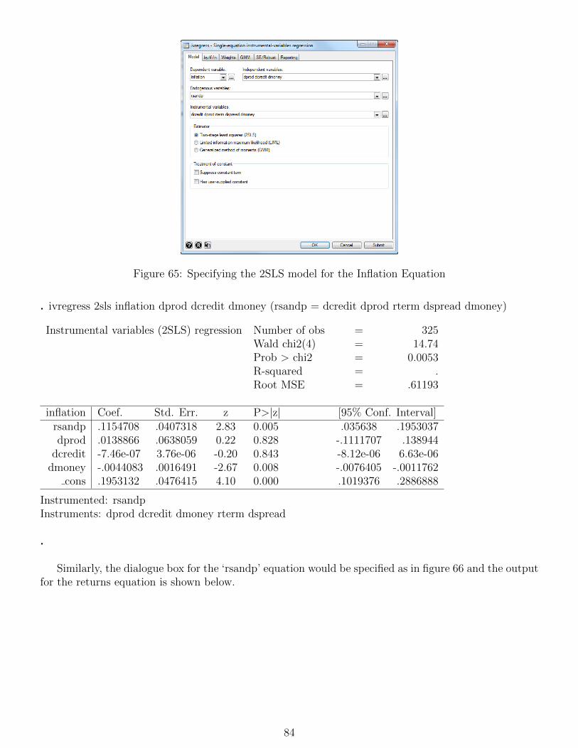
Figure 65: Specifying the 2SLS model for the Inflation Equation

. ivregress 2sls inflation dprod dcredit dmoney (rsandp = dcredit dprod rterm dspread dmoney)

Instrumental variables (2SLS) regression Number of obs = 325Wald chi2(4) = 14.74Prob > chi2 = 0.0053R-squared = .Root MSE = .61193

inflation Coef. Std. Err. z P>|z| [95% Conf. Interval]rsandp .1154708 .0407318 2.83 0.005 .035638 .1953037dprod .0138866 .0638059 0.22 0.828 -.1111707 .138944

dcredit -7.46e-07 3.76e-06 -0.20 0.843 -8.12e-06 6.63e-06dmoney -.0044083 .0016491 -2.67 0.008 -.0076405 -.0011762

cons .1953132 .0476415 4.10 0.000 .1019376 .2886888

Instrumented: rsandpInstruments: dprod dcredit dmoney rterm dspread

.

Similarly, the dialogue box for the ‘rsandp’ equation would be specified as in figure 66 and the outputfor the returns equation is shown below.

84

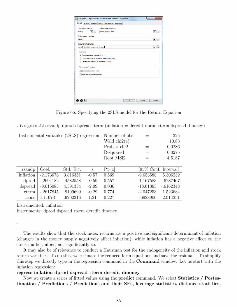
Figure 66: Specifying the 2SLS model for the Return Equation

. ivregress 2sls rsandp dprod dspread rterm (inflation = dcredit dprod rterm dspread dmoney)

Instrumental variables (2SLS) regression Number of obs = 325Wald chi2(4) = 10.83Prob > chi2 = 0.0286R-squared = 0.0275Root MSE = 4.5187

rsandp Coef. Std. Err. z P>|z| [95% Conf. Interval]inflation -2.173678 3.816351 -0.57 0.569 -9.653588 5.306232

dprod -.2694182 .4582558 -0.59 0.557 -1.167583 .6287467dspread -9.615083 4.591334 -2.09 0.036 -18.61393 -.6162348

rterm -.2617845 .9109699 -0.29 0.774 -2.047253 1.523684cons 1.11073 .9202316 1.21 0.227 -.6928906 2.914351

Instrumented: inflationInstruments: dprod dspread rterm dcredit dmoney

.

The results show that the stock index returns are a positive and significant determinant of inflation(changes in the money supply negatively affect inflation), while inflation has a negative effect on thestock market, albeit not significantly so.

It may also be of relevance to conduct a Hausman test for the endogeneity of the inflation and stockreturn variables. To do this, we estimate the reduced form equations and save the residuals. To simplifythis step we directly type in the regression command in the Command window. Let us start with theinflation regression:regress inflation dprod dspread rterm dcredit dmoney

Now we create a series of fitted values using the predict command. We select Statistics / Postes-timation / Predictions / Predictions and their SEs, leverage statistics, distance statistics,

85

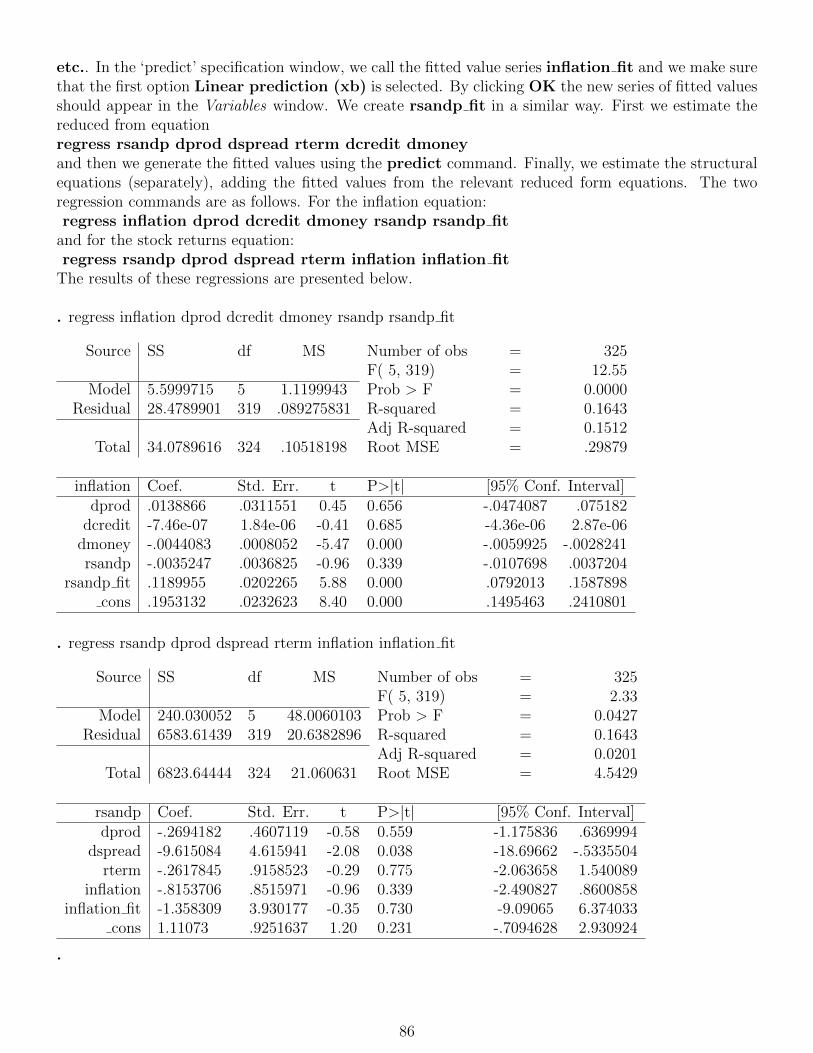
etc.. In the ‘predict’ specification window, we call the fitted value series inflation fit and we make surethat the first option Linear prediction (xb) is selected. By clicking OK the new series of fitted valuesshould appear in the Variables window. We create rsandp fit in a similar way. First we estimate thereduced from equationregress rsandp dprod dspread rterm dcredit dmoneyand then we generate the fitted values using the predict command. Finally, we estimate the structuralequations (separately), adding the fitted values from the relevant reduced form equations. The tworegression commands are as follows. For the inflation equation:regress inflation dprod dcredit dmoney rsandp rsandp fit

and for the stock returns equation:regress rsandp dprod dspread rterm inflation inflation fit

The results of these regressions are presented below.

. regress inflation dprod dcredit dmoney rsandp rsandp fit

Source SS df MS Number of obs = 325F( 5, 319) = 12.55

Model 5.5999715 5 1.1199943 Prob > F = 0.0000Residual 28.4789901 319 .089275831 R-squared = 0.1643

Adj R-squared = 0.1512Total 34.0789616 324 .10518198 Root MSE = .29879

inflation Coef. Std. Err. t P>|t| [95% Conf. Interval]dprod .0138866 .0311551 0.45 0.656 -.0474087 .075182

dcredit -7.46e-07 1.84e-06 -0.41 0.685 -4.36e-06 2.87e-06dmoney -.0044083 .0008052 -5.47 0.000 -.0059925 -.0028241rsandp -.0035247 .0036825 -0.96 0.339 -.0107698 .0037204

rsandp fit .1189955 .0202265 5.88 0.000 .0792013 .1587898cons .1953132 .0232623 8.40 0.000 .1495463 .2410801

. regress rsandp dprod dspread rterm inflation inflation fit

Source SS df MS Number of obs = 325F( 5, 319) = 2.33

Model 240.030052 5 48.0060103 Prob > F = 0.0427Residual 6583.61439 319 20.6382896 R-squared = 0.1643

Adj R-squared = 0.0201Total 6823.64444 324 21.060631 Root MSE = 4.5429

rsandp Coef. Std. Err. t P>|t| [95% Conf. Interval]dprod -.2694182 .4607119 -0.58 0.559 -1.175836 .6369994

dspread -9.615084 4.615941 -2.08 0.038 -18.69662 -.5335504rterm -.2617845 .9158523 -0.29 0.775 -2.063658 1.540089

inflation -.8153706 .8515971 -0.96 0.339 -2.490827 .8600858inflation fit -1.358309 3.930177 -0.35 0.730 -9.09065 6.374033

cons 1.11073 .9251637 1.20 0.231 -.7094628 2.930924

.

86

The conclusion is that the inflation fitted value term is not significant in the stock return equationand so inflation can be considered exogenous for stock returns. Thus it would be valid to simply estimatethis equation (minus the fitted value term) on its own using OLS. But the fitted stock return term issignificant in the inflation equation, suggesting that stock returns are endogenous.

87

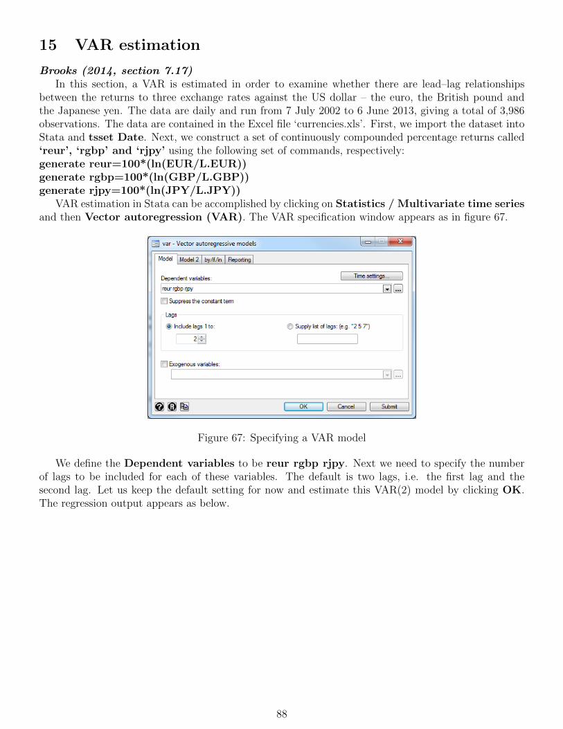
15 VAR estimation

Brooks (2014, section 7.17)In this section, a VAR is estimated in order to examine whether there are lead–lag relationships

between the returns to three exchange rates against the US dollar – the euro, the British pound andthe Japanese yen. The data are daily and run from 7 July 2002 to 6 June 2013, giving a total of 3,986observations. The data are contained in the Excel file ‘currencies.xls’. First, we import the dataset intoStata and tsset Date. Next, we construct a set of continuously compounded percentage returns called‘reur’, ‘rgbp’ and ‘rjpy’ using the following set of commands, respectively:generate reur=100*(ln(EUR/L.EUR))generate rgbp=100*(ln(GBP/L.GBP))generate rjpy=100*(ln(JPY/L.JPY))

VAR estimation in Stata can be accomplished by clicking on Statistics / Multivariate time seriesand then Vector autoregression (VAR). The VAR specification window appears as in figure 67.

Figure 67: Specifying a VAR model

We define the Dependent variables to be reur rgbp rjpy. Next we need to specify the numberof lags to be included for each of these variables. The default is two lags, i.e. the first lag and thesecond lag. Let us keep the default setting for now and estimate this VAR(2) model by clicking OK.The regression output appears as below.

88

. var reur rgbp rjpy, lags(1/2)Vector autoregressionSample: 10jul2002 - 06jun2013 Number of obs = 3985Log likelihood = -6043.54 AIC = 3.043684FPE = .0042115 HQIC = 3.055437Det(Sigma ml) = .0041673 SBIC = 3.076832Equation Parms RMSE R-sq chi2 P>chi2reur 7 .470301 0.0255 104.1884 0.0000rgbp 7 .430566 0.0522 219.6704 0.0000rjpy 7 .466151 0.0243 99.23658 0.0000

Coef. Std. Err. z P>|z| [95% Conf. Interval]reur

reurL1. .2001552 .0226876 8.82 0.000 .1556883 .2446221L2. -.0334134 .0225992 -1.48 0.139 -.077707 .0108802

rgbpL1. -.0615658 .0240862 -2.56 0.011 -.1087738 -.0143578L2. .024656 .0240581 1.02 0.305 -.0224971 .0718091

rjpyL1. -.0201509 .0166431 -1.21 0.226 -.0527707 .0124689L2. -.002628 .0166676 0.16 0.875 -.0300398 .0352958

cons -.0058355 .0074464 -0.78 0.433 -.0204301 .0087591rgbp

reurL1. -.0427769 .0207708 -2.06 0.039 -.0834868 -.0020669L2. .0567707 .0206898 2.74 0.006 .0162194 .097322

rgbpL1. .2616429 .0220512 11.87 0.000 .2184234 .3048623L2. -.0920986 .0220255 -4.18 0.000 -.1352678 -.0489294

rjpyL1. -.0566386 .0152369 -3.72 0.000 -.0865024 -.0267747L2. .0029643 .0152593 0.19 0.846 -.0269435 .0328721

cons .0000454 .0068172 0.01 0.995 -.0133161 .0134069rjpy

reurL1. .0241862 .0224874 1.08 0.282 -.0198883 .0682607L2. -.0313338 .0223997 -1.40 0.162 -.0752365 .0125689

rgbpL1. -.0679786 .0238736 -2.85 0.004 -.1147701 -.0211872L2. .0324034 .0238458 1.36 0.174 -.0143336 .0791404

rjpyL1. .1508446 .0164962 9.14 0.000 .1185127 .1831766L2. .0007184 .0165205 0.04 0.965 -.0316611 .0330979

cons -.0036822 .0073807 -0.50 0.618 -.0181481 .0107836

.

At the top of the table, we find information for the model as a whole, inluding information criteria,while further down we find coefficient estimates and goodness-of-fit measures for each of the equationsseparately. Each regression equation is separated by a horizontal line.

We will shortly discuss the interpretation of the output, but the example so far has assumed that we

89

know the appropriate lag length for the VAR. However, in practice, the first step in the construction ofany VAR model, once the variables that will enter the VAR have been decided, will be to determine theappropriate lag length. This can be achieved in a variety of ways, but one of the easiest is to employ amultivariate information criterion. In Stata, this can be done by clicking on Statistics / Multivariatetime series / VAR diagnostics and tests and selecting the first option Lag-order selectionstatistics (preestimation). In the specification window we define the Dependent variables: reurrgbp rjpy (figure 68).

Figure 68: Selecting the VAR Lag Order Length

Then we are asked to specify the Maximum Lag order to entertain including in the model, and forthis example, we arbitrarily select 10. By clicking OK we should be able to observe the following output.

. varsoc reur rgbp rjpy, maxlag(10)

Selection-order criteriaSample: 18jul2002 - 06jun2013 Number of obs = 3977

lag LL LR df p FPE AIC HQIC SBIC

0 -6324.33 .004836 3.18196 3.18364 3.186711 -6060.26 528.13 9 0.000 .004254 3.05369 3.06042 3.07266*2 -6034.87 50.784 9 0.000 .004219* 3.04545* 3.05722* 3.078653 -6030.96 7.8286 9 0.552 .00423 3.048 3.06482 3.095444 -6022.94 16.04 9 0.066 .004232 3.0485 3.07036 3.110165 -6015.11 15.655 9 0.074 .004234 3.04909 3.076 3.124986 -6009.17 11.881 9 0.220 .004241 3.05063 3.08258 3.140757 -6000.17 17.998* 9 0.035 .004241 3.05063 3.08763 3.154988 -5992.97 14.408 9 0.109 .004245 3.05153 3.09358 3.170129 -5988.13 9.6673 9 0.378 .004254 3.05362 3.10072 3.18644

10 -5984.25 7.7658 9 0.558 .004264 3.0562 3.10834 3.20325

Endogenous: reur rgbp rjpyExogenous: cons

90

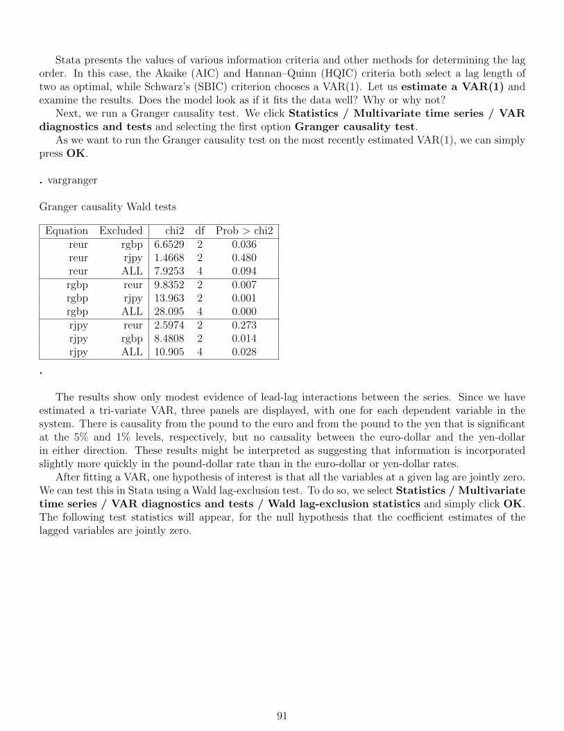
Stata presents the values of various information criteria and other methods for determining the lagorder. In this case, the Akaike (AIC) and Hannan–Quinn (HQIC) criteria both select a lag length oftwo as optimal, while Schwarz’s (SBIC) criterion chooses a VAR(1). Let us estimate a VAR(1) andexamine the results. Does the model look as if it fits the data well? Why or why not?

Next, we run a Granger causality test. We click Statistics / Multivariate time series / VARdiagnostics and tests and selecting the first option Granger causality test.

As we want to run the Granger causality test on the most recently estimated VAR(1), we can simplypress OK.

. vargranger

Granger causality Wald tests

Equation Excluded chi2 df Prob > chi2reur rgbp 6.6529 2 0.036reur rjpy 1.4668 2 0.480reur ALL 7.9253 4 0.094rgbp reur 9.8352 2 0.007rgbp rjpy 13.963 2 0.001rgbp ALL 28.095 4 0.000rjpy reur 2.5974 2 0.273rjpy rgbp 8.4808 2 0.014rjpy ALL 10.905 4 0.028

.

The results show only modest evidence of lead-lag interactions between the series. Since we haveestimated a tri-variate VAR, three panels are displayed, with one for each dependent variable in thesystem. There is causality from the pound to the euro and from the pound to the yen that is significantat the 5% and 1% levels, respectively, but no causality between the euro-dollar and the yen-dollarin either direction. These results might be interpreted as suggesting that information is incorporatedslightly more quickly in the pound-dollar rate than in the euro-dollar or yen-dollar rates.

After fitting a VAR, one hypothesis of interest is that all the variables at a given lag are jointly zero.We can test this in Stata using a Wald lag-exclusion test. To do so, we select Statistics / Multivariatetime series / VAR diagnostics and tests / Wald lag-exclusion statistics and simply click OK.The following test statistics will appear, for the null hypothesis that the coefficient estimates of thelagged variables are jointly zero.

91

. varwle

Equation: reur

lag chi2 df Prob > chi21 104.0216 3 0.0002 2.222079 3 0.528

Equation: rgbp

lag chi2 df Prob > chi21 214.893 3 0.0002 17.60756 3 0.001

Equation: rjpy

lag chi2 df Prob > chi21 95.98737 3 0.0002 2.298777 3 0.513

Equation: All

lag chi2 df Prob > chi21 592.6466 9 0.0002 51.14752 9 0.000

.

Stata obtains these test statistics for each of the three equations separately (first three panels) andfor all three equations jointly (last panel). Based on the high χ2 values for all four panels, we havestrong evidence that we can reject the null so that no lags should be excluded.

To obtain the impulse responses for the estimated model, we click on Statistics / Multivariatetime series / Basic VAR. We are then presented with a specification window, as in figure 69.

Figure 69: Generating Impulse Responses for the VAR(1) model

We define the Dependent variables: reur rgbp rjpy and select a VAR model with one lag ofeach variable. We can do this either by specifying Include lags 1 to: 1 or by Supply list of lags:

92

1. We then specify that we want to generate a Graph for the IRFs, that is the impulse responsefunctions. Finally, we need to select the number of periods over which we want to generate the IRFs.We arbitrarily select 20 and press OK. You can see that Stata re-estimates the VAR(1) but additionallyit creates a set of graphs of the implied IRFs (figure 70).

Figure 70: Graphs of Impulse Response Functions (IRFs) for the VAR(1) model

As one would expect given the parameter estimates and the Granger causality test results, only afew linkages between the series are established here. The responses to the shocks are very small, exceptfor the response of a variable to its own shock, and they die down to almost nothing after the first lag.

Note that plots of the variance decompositions can also be generated using the varbasic command.Instead of specifying the IRFs in the Graph selection, we choose FEVDs, that is the forecast-errorvariance decompositions. A similar plot for the variance decompositions would appear as in figure 71.

There is little again that can be seen from these variance decomposition graphs apart from thefact that the behaviour is observed to settle down to a steady state very quickly. To illustrate how tointerpret the FEVDs, let us have a look at the effect that a shock to the euro rates has on the other tworates and itself, which are shown in the first row of the FEVD plot. Interestingly, while the percentageof the errors that are attributable to own shocks is 100% in the case of the euro rate (top left graph),for the pound, the euro series explains around 47% of the variation in returns (top middle graph), andfor the yen, the euro series explains around 7% of the variation.

We should remember that the ordering of the variables has an effect on the impulse responses andvariance decompositions, and when, as in this case, theory does not suggest an obvious ordering ofthe series, some sensitivity analysis should be undertaken. Let us assume we would like to test howsensitive the FEVDs are to a different way of ordering. We first click on Statistics / Multivariatetime series and select IRF and FEVD analysis / Obtain IRFs, dynamic-multiplier functions,and FEVDs.

93

Figure 71: Graphs of FEVDs for the VAR(1) model

Figure 72: Generating FEVDs for an alternative ordering

94

In the specification window that appears, we first need to Set active IRF file... which we do bysimply clicking on the respective button and then pressing OK (figure 72). You can see that in the folderwhere the current workfile is stored a new file appears named varbasic.irf which will store all the newIRF results. However, you do not need to concern yourself with this file as Stata will automaticallyobtain the necessary information from the files if needed. Next we name the new IRF as order2. Tomake our results comparable, we choose 20 Forecast horizon. Finally, we need to select the order ofthe variables. In this test, we choose the reverse order to that used previously, which isrjpy rgbp reurand click OK to generate the IRFs. To inspect and compare the FEVDs for this ordering and theprevious one, we can create graphs of the FEVDs by selecting Statistics / Multivariate time series/ IRF and FEVD analysis / Graphs by impulse or response. A specification window as shownin figure 73, upper panel, appears. We only need to specify the Statistics to graph which is Choleskyforecast-error variance decomposition (fevd) and click OK. We can now compare the FEVDs ofthe reverse order with those of the previous ordering (figure 73, lower panel). Note that the FEVDs forthe original order are denoted by ‘varbasic’ and the ones for the reverse ordering by ‘order2’.

95

Figure 73: Graphs for FEVDs with an alternative ordering

96

16 Testing for unit roots

Brooks (2014, section 8.3)In this section, we focus on how we can test whether a data series is stationary or not using Stata.

This example uses the same data on UK house prices as employed previously (‘ukhp.dta’). Assumingthat the data have been loaded, and the variables are defined as before, we want to conduct a unit roottest on the HP series. We click on Statistics / Time series / Tests and can select from a numberof different unit root tests. To start with, we choose the first option Augmented Dickey-Fullerunit-root test. In the test specification window, we select Variable: HP and select 10 Laggeddifferences to be included in the test (figure 74).

Figure 74: Specifying an Augmented Dickey-Fuller Test for Unit Roots

We can also select whether we would like to show the regression results from the auxiliary regressionby checking the box Display regression table. We press OK and the following test statistics arereported in the Output window on the next page.

In the upper part of the output we find the actual test statistics for the null hypothesis that theseries ‘HP’ has a unit root. Clearly, the test statistic (−0.610) is not more negative than the criticalvalue, so the null hypothesis of a unit root in the house price series cannot be rejected. The remainderof the output presents the estimation results. Since one of the independent variables in this regressionis non-stationary, it is not appropriate to examine the coefficient standard errors or their t-ratios in thetest regression.. dfuller HP, regress lags(10)

Augmented Dickey-Fuller test for unit root Number of obs = 258

———– Interpolated Dickey-Fuller ———–Test 1% Critical 5% Critical 10% Critical

Statistic Value Value Value

Z(t) -0.610 -3.459 -2.880 -2.570

MacKinnon approximate p-value for Z(t) = 0.8687

97

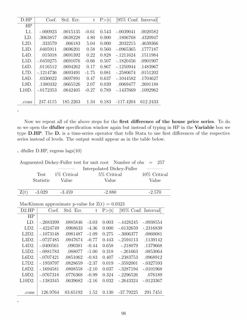
D.HP Coef. Std. Err. t P>|t| [95% Conf. Interval]HPL1. -.000923 .0015135 -0.61 0.543 -.0039041 .0020582LD. .3063857 .0638228 4.80 0.000 .1806768 .4320947

L2D. .333579 .066183 5.04 0.000 .2032215 .4639366L3D. .0405911 .0696201 0.58 0.560 -.0965365 .1777187L4D. .015018 .0691392 0.22 0.828 -.1211624 .1511984L5D. -.0459275 .0691076 -0.66 0.507 -.1820456 .0901907L6D. .0116512 .0694262 0.17 0.867 -.1250944 .1483967L7D. -.1214736 .0693491 -1.75 0.081 -.2580674 .0151202L8D. .0330022 .0697891 0.47 0.637 -.1044582 .1704627L9D. .1380332 .0665526 2.07 0.039 .0069477 .2691188

L10D. -.0172353 .0642405 -0.27 0.789 -.1437669 .1092962

cons 247.4115 185.2263 1.34 0.183 -117.4204 612.2433

.

Now we repeat all of the above steps for the first difference of the house price series. To doso we open the dfuller specification window again but instead of typing in HP in the Variable box wetype D.HP. The D. is a time-series operator that tells Stata to use first differences of the respectiveseries instead of levels. The output would appear as in the table below.

. dfuller D.HP, regress lags(10)

Augmented Dickey-Fuller test for unit root Number of obs = 257

———– Interpolated Dickey-Fuller ———–Test 1% Critical 5% Critical 10% Critical

Statistic Value Value Value

Z(t) -3.029 -3.459 -2.880 -2.570

MacKinnon approximate p-value for Z(t) = 0.0323

D2.HP Coef. Std. Err. t P>|t| [95% Conf. Interval]HPLD. -.2683399 .0885846 -3.03 0.003 -.4428245 -.0938554

LD2. -.4224749 .0968633 -4.36 0.000 -.6132659 -.2316839L2D2. -.1073148 .0981487 -1.09 0.275 -.3006377 .0860081L3D2. -.0727485 .0947674 -0.77 0.443 -.2594113 .1139142L4D2. -.0400561 .090381 -0.44 0.658 -.218079 .1379668L5D2. -.0881783 .088077 -1.00 0.318 -.261663 .0853064L6D2. -.0707421 .0851062 -0.83 0.407 -.2383753 .0968912L7D2. -.1959797 .0828659 -2.37 0.019 -.3592001 -.0327593L8D2. -.1694581 .0808558 -2.10 0.037 -.3287194 -.0101968L9D2. -.0767318 .0776368 -0.99 0.324 -.2296526 .076189

L10D2. -.1383345 .0639682 -2.16 0.032 -.2643324 -.0123367

cons 126.9764 83.65192 1.52 0.130 -37.79225 291.7451

.

98

We find that the null hypothesis of a unit root can be rejected for the differenced house price seriesat the 5% level.48

For completeness, we run a unit root test on the dhp series (levels, not differenced), which are thepercentage changes rather than the absolute differences in prices. We should find that these are alsostationary (at the 5% level for a lag length of 10).

As mentioned above, Stata presents a large number of options for unit root tests. We could forexample include a trend term or a drift term in the ADF regression. Alternatively, we can use acompletely different test setting – for example, instead of the Dickey–Fuller test, we could run thePhillips–Perron test for stationarity. Among the options available in Stata, we only focus on one furtherunit root test that is strongly related to the Augmented Dickey-Fuller test presented above, namely theDickeyFuller GLS test (dfgls). It can be accessed in Stata via Statistics / Time series / DF-GLStest for a unit root. ‘dfgls’ performs a modified DickeyFuller t-test for a unit root in which the serieshas been transformed by a generalized least-squares regression. Several empirical studies have shownthat this test has significantly greater power than the previous versions of the augmented DickeyFullertest. Another advantage of the ‘dfgls’ test is that it does not require knowledge of the optimal lag lengthbefore running it but it performs the test for a series of models that include 1 to k lags.

Figure 75: Specifying the Dickey-Fuller GLS test

In the specification window, shown in figure 75, we select Variable: HP and specify the Highestlag order for Dickey-Fuller GLS regressions to be 10. We then press OK and Stata generates thefollowing output.

48If we decrease the number of added lags we find that the null hypothesis is rejected even at the 1% significance level.Please feel free to re-estimate the ADF test for varying lag lengths.

99

. dfgls HP, maxlag(10)

DF-GLS for HP Number of obs = 258

DF-GLS tau 1% Critical 5% Critical 10% Critical[lags] Test Statistic Value Value Value

10 -1.485 -3.480 -2.851 -2.5689 -1.510 -3.480 -2.859 -2.5758 -1.318 -3.480 -2.866 -2.5827 -1.227 -3.480 -2.873 -2.5886 -1.304 -3.480 -2.880 -2.5945 -1.275 -3.480 -2.887 -2.6004 -1.348 -3.480 -2.893 -2.6063 -1.349 -3.480 -2.899 -2.6112 -1.310 -3.480 -2.904 -2.6161 -0.893 -3.480 -2.910 -2.621

Opt Lag (Ng-Perron seq t) = 9 with RMSE 1168.4Min SC = 14.22293 at lag 2 with RMSE 1186.993Min MAIC = 14.1874 at lag 2 with RMSE 1186.993

.We see a series of test statistics for models with different lag length, from 10 lags to 1 lag. Below

the table we find information criteria in order to select the optimal lag length. The last two criteria,the modified Schwartz criterion (Min SC) and the modified Akaike information criterion (MAIC), bothselect an optimal lag length of 2.

100

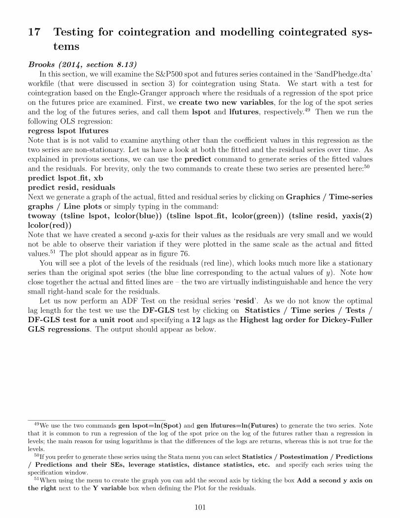
17 Testing for cointegration and modelling cointegrated sys-

tems

Brooks (2014, section 8.13)In this section, we will examine the S&P500 spot and futures series contained in the ‘SandPhedge.dta’

workfile (that were discussed in section 3) for cointegration using Stata. We start with a test forcointegration based on the Engle-Granger approach where the residuals of a regression of the spot priceon the futures price are examined. First, we create two new variables, for the log of the spot seriesand the log of the futures series, and call them lspot and lfutures, respectively.49 Then we run thefollowing OLS regression:regress lspot lfuturesNote that is is not valid to examine anything other than the coefficient values in this regression as thetwo series are non-stationary. Let us have a look at both the fitted and the residual series over time. Asexplained in previous sections, we can use the predict command to generate series of the fitted valuesand the residuals. For brevity, only the two commands to create these two series are presented here:50

predict lspot fit, xbpredict resid, residualsNext we generate a graph of the actual, fitted and residual series by clicking on Graphics / Time-seriesgraphs / Line plots or simply typing in the command:twoway (tsline lspot, lcolor(blue)) (tsline lspot fit, lcolor(green)) (tsline resid, yaxis(2)lcolor(red))Note that we have created a second y-axis for their values as the residuals are very small and we wouldnot be able to observe their variation if they were plotted in the same scale as the actual and fittedvalues.51 The plot should appear as in figure 76.

You will see a plot of the levels of the residuals (red line), which looks much more like a stationaryseries than the original spot series (the blue line corresponding to the actual values of y). Note howclose together the actual and fitted lines are – the two are virtually indistinguishable and hence the verysmall right-hand scale for the residuals.

Let us now perform an ADF Test on the residual series ‘resid’. As we do not know the optimallag length for the test we use the DF-GLS test by clicking on Statistics / Time series / Tests /DF-GLS test for a unit root and specifying a 12 lags as the Highest lag order for Dickey-FullerGLS regressions. The output should appear as below.

49We use the two commands gen lspot=ln(Spot) and gen lfutures=ln(Futures) to generate the two series. Notethat it is common to run a regression of the log of the spot price on the log of the futures rather than a regression inlevels; the main reason for using logarithms is that the differences of the logs are returns, whereas this is not true for thelevels.

50If you prefer to generate these series using the Stata menu you can select Statistics / Postestimation / Predictions/ Predictions and their SEs, leverage statistics, distance statistics, etc. and specify each series using thespecification window.

51When using the menu to create the graph you can add the second axis by ticking the box Add a second y axis onthe right next to the Y variable box when defining the Plot for the residuals.

101

Figure 76: Actual, Fitted and Residual Plot

. dfgls resid, maxlag(12)

DF-GLS for resid Number of obs = 122

DF-GLS tau 1% Critical 5% Critical 10% Critical[lags] Test Statistic Value Value Value

12 -1.344 -3.538 -2.793 -2.51811 -1.276 -3.538 -2.814 -2.53810 -1.309 -3.538 -2.835 -2.5579 -1.472 -3.538 -2.855 -2.5768 -1.244 -3.538 -2.875 -2.5947 -1.767 -3.538 -2.894 -2.6116 -1.656 -3.538 -2.911 -2.6285 -1.448 -3.538 -2.928 -2.6434 -1.858 -3.538 -2.944 -2.6583 -2.117 -3.538 -2.959 -2.6712 -2.168 -3.538 -2.973 -2.6841 -4.274 -3.538 -2.985 -2.695

Opt Lag (Ng-Perron seq t) = 9 with RMSE .0020241Min SC = -12.07091 at lag 2 with RMSE .0022552Min MAIC = -12.1927 at lag 8 with RMSE .0020542

.The three information criteria at the botton of the test output all suggest a different optimal lag

length. Let us focus on the minimum Schwarz information criterion (Min SC) for now which suggegstsan optimal lag length of 2. For two lags we have a test statistic of (−2.168) which is not more negativethan the critical values, even at the 10% level. Thus, the null hypothesis of a unit root in the testregression residuals cannot be rejected and we would conclude that the two series are not cointegrated.This means that the most appropriate form of the model to estimate would be one containing only firstdifferences of the variables as they have no long-run relationship.

If instead we had found the two series to be cointegrated, an error correction model (ECM) couldhave been estimated, as there would be a linear combination of the spot and futures prices that would

102

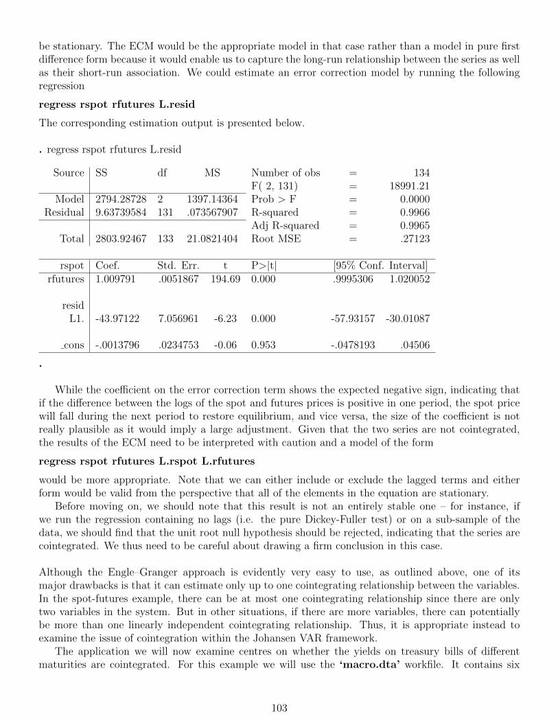
be stationary. The ECM would be the appropriate model in that case rather than a model in pure firstdifference form because it would enable us to capture the long-run relationship between the series as wellas their short-run association. We could estimate an error correction model by running the followingregression

regress rspot rfutures L.resid

The corresponding estimation output is presented below.

. regress rspot rfutures L.resid

Source SS df MS Number of obs = 134F( 2, 131) = 18991.21

Model 2794.28728 2 1397.14364 Prob > F = 0.0000Residual 9.63739584 131 .073567907 R-squared = 0.9966

Adj R-squared = 0.9965Total 2803.92467 133 21.0821404 Root MSE = .27123

rspot Coef. Std. Err. t P>|t| [95% Conf. Interval]rfutures 1.009791 .0051867 194.69 0.000 .9995306 1.020052

residL1. -43.97122 7.056961 -6.23 0.000 -57.93157 -30.01087

cons -.0013796 .0234753 -0.06 0.953 -.0478193 .04506

.

While the coefficient on the error correction term shows the expected negative sign, indicating thatif the difference between the logs of the spot and futures prices is positive in one period, the spot pricewill fall during the next period to restore equilibrium, and vice versa, the size of the coefficient is notreally plausible as it would imply a large adjustment. Given that the two series are not cointegrated,the results of the ECM need to be interpreted with caution and a model of the form

regress rspot rfutures L.rspot L.rfutures

would be more appropriate. Note that we can either include or exclude the lagged terms and eitherform would be valid from the perspective that all of the elements in the equation are stationary.

Before moving on, we should note that this result is not an entirely stable one – for instance, ifwe run the regression containing no lags (i.e. the pure Dickey-Fuller test) or on a sub-sample of thedata, we should find that the unit root null hypothesis should be rejected, indicating that the series arecointegrated. We thus need to be careful about drawing a firm conclusion in this case.

Although the Engle–Granger approach is evidently very easy to use, as outlined above, one of itsmajor drawbacks is that it can estimate only up to one cointegrating relationship between the variables.In the spot-futures example, there can be at most one cointegrating relationship since there are onlytwo variables in the system. But in other situations, if there are more variables, there can potentiallybe more than one linearly independent cointegrating relationship. Thus, it is appropriate instead toexamine the issue of cointegration within the Johansen VAR framework.

The application we will now examine centres on whether the yields on treasury bills of differentmaturities are cointegrated. For this example we will use the ‘macro.dta’ workfile. It contains six

103

interest rate series corresponding to 3 and 6 months, and 1, 3, 5, and 10 years.52 Each series has a namein the file starting with the letters ‘USTB’. The first step in any cointegration analysis is to ensure thatthe variables are all non-stationary in their levels form, so confirm that this is the case for each ofthe six series, by running a unit root test on each one using the dfgls command with a maximum laglength of 12.53

Before specifying the VECM using the Johansen method, it is often very useful to graph the variablesto see how they are behaving over time and with respect to each other. This will also help us to selectthe correct option for the VECM specification, e.g. if the series appear to follow a linear trend. Togenerate a graph of all variables we use the well-known time-series line plot:twoway (tsline USTB3M) (tsline USTB6M) (tsline USTB1Y) (tsline USTB3Y) (tslineUSTB5Y) (tsline USTB10Y)and figure 77 should appear.

Figure 77: Graph of the six U.S. Treasury Interest Rates

We see that the series generally follow a linear downward trend, though some series show strongerinter-temporal variation with large drops than other series. Additionally, while all series seem to berelated in some way, we find that the plots of some rates resemble each other more strictly than others,e.g. the USTB3M, USTB6M and USTB1Y rates.

To test for cointegration or fit cointegrating VECMs, we must also specify how many lags to includein the model. To select the optimal number of lags we can use the methods implemented in Stata’svarsoc command. To access this test, we click on Statistics / Multivariate time series / VECdiagnostics and tests / Lag-order selection statistics (preestimation). However, as the modelswe are planning to estimate are very large, we need to increase the maximum number of variables thatStata allows in a model, the so-called matsize. The default matsize is 400, while the maximum matsize inStata/MP and Stata/SE is 11,000. We simply set matsize to its maximum number using the command:set matsize 11000Once this is done, we can run the lag-order selection test. In the specification window for the test, wefirst define all the six interest rates as Dependent variables and then select a Maximum lagorder of 12 (figure 78). We then click OK and the test output should appear as below.

52The vec intro entry in the Stata Manual provides a good overview of estimating vector error-correction models inStata. It illustrates the process of testing for cointegration and estimating a VECM based on an example.

53Note that for the 3-year, 5-year and 10-year rates the unit root test is rejected for the optimal lag length based onthe Schwarz criterion. However, for the sake of this example we will continue using all of the six rates.

104

Figure 78: Specifying the lag-order selection test

. varsoc USTB3M USTB6M USTB1Y USTB3Y USTB5Y USTB10Y, maxlag(12)

Selection-order criteriaSample: 1987m3 - 2013m4 Number of obs = 314

lag LL LR df p FPE AIC HQIC SBIC0 -32.6156 5.2e-08 .245959 .274587 .3176041 1820.03 3705.3 36 0.000 4.9e-13 -11.3251 -11.1247* -10.8235*2 1879.97 119.86 36 0.000 4.2e-13 -11.4775 -11.1053 -10.54613 1922.26 84.579 36 0.000 4.0e-13* -11.5176* -10.9736 -10.15634 1950.23 55.95 36 0.018 4.2e-13 -11.4664 -10.7507 -9.675335 1983.36 66.264 36 0.002 4.3e-13 -11.4482 -10.5607 -9.227196 2013.46 60.195 36 0.007 4.5e-13 -11.4106 -10.3513 -8.759737 2037.92 48.924 36 0.074 4.9e-13 -11.3371 -10.1061 -8.256378 2067.96 60.082 36 0.007 5.1e-13 -11.2991 -9.89637 -7.788559 2099.03 62.137 36 0.004 5.3e-13 -11.2677 -9.69319 -7.32727

10 2126.11 54.153* 36 0.027 5.6e-13 -11.2109 -9.46458 -6.8405711 2149.28 46.349 36 0.116 6.2e-13 -11.1292 -9.21113 -6.3290112 2165.15 31.727 36 0.672 7.1e-13 -11.0009 -8.9111 -5.77089

Endogenous: USTB3M USTB6M USTB1Y USTB3Y USTB5Y USTB10YExogenous: cons

.

The four information criteria provide inconclusive results regarding the optimal lag length. Whilethe FPE and the AIC suggest an optimal lag length of 3 lags, the HQIC and SBIC favour a lag lengthof 1. Note that the difference in optimal model order could be attributed to the relatively small samplesize available with this monthly sample compared with the number of observations that would havebeen available were daily data used, implying that the penalty term in SBIC is more severe on extraparameters in this case. In the framework of this example, we follow the AIC and select a lag length of

105

Figure 79: Testing for the number of cointegrating relationships

three.The next step of fitting a VECM is determining the number of cointegrating relationships using a

VEC rank test. The corresponding Stata command is vecrank. The tests for cointegration implementedin ‘vecrank’ are based on Johansen’s method by comparing the log likelihood functions for a modelthat contains the cointegraing equation(s) and a model that does not. If the log likelihood of theunconstrained model that includes the cointegrating equations is significantly different from the loglikelihood of the constrained model that does not include the cointegrating equations, we reject the nullhypothesis of no cointegration.

To access the VEC rank test, we click on Statistics / Multivariate time series and selectCointegrating rank of a VECM. First we define the list of Dependent variables:USTB3M USTB6M USTB1Y USTB3Y USTB5Y USTB10Y

Next, we set the Maximum lag to be included in the underlying VAR model to 3 as de-termined in the previous step. We leave the Trend specification unchanged as based upon the visualinspection of the data series, they roughly seemed to follow a linear downward trend. By clicking OKin the box completed as in figure 79, the following output should appear in the Output window.

. vecrank USTB3M USTB6M USTB1Y USTB3Y USTB5Y USTB10Y, trend(constant) lags(3)Johansen tests for cointegration

Trend: constant Number of obs = 323Sample: 1986m6 - 2013m4 Lags = 3

5%maximum trace critical

rank parms LL eigenvalue statistic value0 78 1892.2945 . 158.5150 94.151 89 1923.5414 0.17591 96.0211 68.522 98 1943.6204 0.11691 55.8632 47.213 105 1960.5828 0.09970 21.9384* 29.684 110 1967.1992 0.04014 8.7056 15.415 113 1970.9016 0.02266 1.3007 3.766 114 1971.552 0.00402

.

106

The first column in the table shows the rank of the VECM that is been tested or in other words thenumber of cointegrating relationships for the set of interest rates. The second and third columns reportthe number of smoothing parameters and the log-likelihood values, respectively. In the fourth columnwe find the ordered eigenvalues, from highest to lowest. We find the λtrace statistics in the fifth column,together with the corresponding critical values. The first row of the table tests the null hypothesis ofno cointegrating vectors, against the alternative hypothesis that the number of cointegrating equationsis strictly larger than the number assumed under the null hypothesis, i.e. larger than zero. The teststatistic of 158.5150 considerably exceeds the critical value (94.15) and so the null of no cointegratingvectors is rejected. If we then move to the next row, the test statistic (96.0211) again exceeds the criticalvalue so that the null of at most one cointegrating vector is also rejected. This continues, and we alsoreject the null of at most two cointegrating vectors, but we stop at the next row, where we do not rejectthe null hypothesis of at most three cointegrating vectors at the 5% level, and this is the conclusion.

Besides the λtrace statistic, we can also employ an alternative statistic, the maximum-eigenvaluestatistic (λmax). In contrast to the trace statistic, the maximum-eigenvalue statistic assumes a givennumber of r cointegrating relations under the null hypothesis and test this against the alternative thatthere are r+1 cointegrating equations. We can generate the results for this alternative test by going backto the ‘vecrank’ specification window, changing to the Reporting tab and checking the box Reportmaximum-eigenvalue statistic. We leave everything else unchanged and click OK.

The test output should now report the results for the λtrace statistics in the first panel and those forthe λmax statistics in the panel below. We find that the results from the λmax test confirm our previousresults of three cointegrating relations between the interest rates.

Figure 80: Specifying the VECM

Now that we have determined the lag length, trend specification and the number of cointegratingrelationships, we can fit the VECM model. To do so, we click on Statistics / Multivariate timeseries and select Vector error-correction model (VECM). In the VECM specification window,we first specify the six interest rates as the Dependent variables and then select 3 as the Numberof cointegrating equations (rank) and 3 again as the Maximum lag to be included in theunderlying VAR model (figure 80). As in the previous specification, we keep the default Trendspecification: constant as well as all other default specifications and simply press OK. The followingoutput shall appear in the Output window.

107

. vec USTB3M USTB6M USTB1Y USTB3Y USTB5Y USTB10Y, trend(constant) rank(3) lags(3)

Vector error-correction modelSample: 1986m6 - 2013m4 No. of obs = 323

AIC = -11.48968Log likelihood = 1960.583 HQIC = -10.99946Det(Sigma ml) = 2.15e-13 SBIC = -10.26165

Equation Parms RMSE R-sq chi2 P>chi2

D USTB3M 16 .204023 0.2641 109.7927 0.0000D USTB6M 16 .21372 0.2298 91.29766 0.0000D USTB1Y 16 .243715 0.1554 56.3156 0.0000D USTB3Y 16 .29857 0.0751 24.86329 0.0723D USTB5Y 16 .300126 0.0820 27.31828 0.0381D USTB10Y 16 .278729 0.0960 32.48449 0.0086

Coef. Std. Err. z P>|z| [95% Conf. Interval]D USTB3M

ce1L1. -.4569657 .1467312 -3.11 0.002 -.7445536 -.1693778ce2L1. .5265096 .2781872 1.89 0.058 -.0187272 1.071747ce3L1. -.2533181 .214998 -1.18 0.239 -.6747064 .1680703

USTB3MLD. .276511 .1727198 1.60 0.109 -.0620137 .6150357

L2D. .2055372 .16444 1.25 0.211 -.1167593 .5278338USTB6M

LD. -.6069326 .3246052 -1.87 0.062 -1.243147 .0292819L2D. .1797348 .294343 0.61 0.541 -.3971669 .7566364

USTB1YLD. .44994 .2866458 1.57 0.116 -.1118755 1.011755

L2D. -.4549915 .257482 -1.77 0.077 -.9596469 .049664USTB3Y

LD. .17893 .2930182 0.61 0.541 -.3953752 .7532352L2D. .2757354 .2737646 1.01 0.314 -.2608334 .8123042

USTB5YLD. -.1275342 .3269614 -0.39 0.696 -.7683668 .5132984

L2D. .0650113 .3105497 0.21 0.834 -.543655 .6736776USTB10Y

LD. -.0484528 .166626 -0.29 0.771 -.3750339 .2781282L2D. -.2022248 .1619594 -1.25 0.212 -.5196593 .1152097cons -.0019721 .0128153 -0.15 0.878 -.0270896 .0231454

108

D USTB6Mce1L1. -.0536696 .1537053 -0.35 0.727 -.3549265 .2475872ce2L1. -.1131205 .2914093 -0.39 0.698 -.6842723 .4580313ce3L1. -.0084675 .2252168 -0.04 0.970 -.4498843 .4329493

USTB3MLD. .2044083 .1809291 1.13 0.259 -.1502063 .5590229

L2D. .1662804 .1722558 0.97 0.334 -.1713347 .5038956USTB6M

LD. -.3504905 .3400336 -1.03 0.303 -1.016944 .3159631L2D. .3979498 .308333 1.29 0.197 -.2063718 1.002271

USTB1YLD. .2241559 .30027 0.75 0.455 -.3643624 .8126743

L2D. -.639109 .26972 -2.37 0.018 -1.167751 -.1104674USTB3Y

LD. .1500058 .3069453 0.49 0.625 -.4515959 .7516076L2D. .3049368 .2867766 1.06 0.288 -.2571349 .8670086

USTB5YLD. .0414401 .3425018 0.12 0.904 -.6298511 .7127312

L2D. -.0189402 .3253101 -0.06 0.954 -.6565361 .6186558USTB10Y

LD. -.1189244 .1745457 -0.68 0.496 -.4610277 .223179L2D. -.1199968 .1696572 -0.71 0.479 -.4525189 .2125252cons .002021 .0134244 0.15 0.880 -.0242903 .0283323

D USTB1Yce1L1. -.0319126 .1752773 -0.18 0.856 -.3754498 .3116246ce2L1. .0235487 .3323076 0.07 0.944 -.6277622 .6748596ce3L1. -.2068419 .2568252 -0.81 0.421 -.71021 .2965262

USTB3MLD. .06837 .2063219 0.33 0.740 -.3360135 .4727535

L2D. .1408624 .1964313 0.72 0.473 -.2441359 .5258607USTB6M

LD. -.0191462 .3877561 -0.05 0.961 -.7791342 .7408418L2D. .3701158 .3516065 1.05 0.293 -.3190202 1.059252

USTB1YLD. -.0049684 .3424118 -0.01 0.988 -.6760833 .6661464

L2D. -.6459894 .3075743 -2.10 0.036 -1.248824 -.0431548USTB3Y

LD. .1905576 .350024 0.54 0.586 -.4954768 .876592L2D. .3026243 .3270246 0.93 0.355 -.3383322 .9435808

USTB5YLD. .0331161 .3905707 0.08 0.932 -.7323884 .7986205

L2D. -.0097814 .3709662 -0.03 0.979 -.7368617 .717299

109

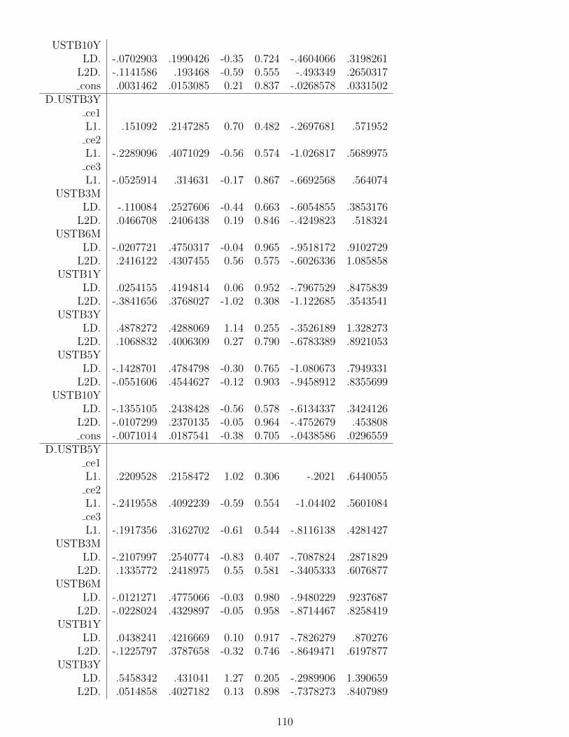
USTB10YLD. -.0702903 .1990426 -0.35 0.724 -.4604066 .3198261

L2D. -.1141586 .193468 -0.59 0.555 -.493349 .2650317cons .0031462 .0153085 0.21 0.837 -.0268578 .0331502

D USTB3Yce1L1. .151092 .2147285 0.70 0.482 -.2697681 .571952ce2L1. -.2289096 .4071029 -0.56 0.574 -1.026817 .5689975ce3L1. -.0525914 .314631 -0.17 0.867 -.6692568 .564074

USTB3MLD. -.110084 .2527606 -0.44 0.663 -.6054855 .3853176

L2D. .0466708 .2406438 0.19 0.846 -.4249823 .518324USTB6M

LD. -.0207721 .4750317 -0.04 0.965 -.9518172 .9102729L2D. .2416122 .4307455 0.56 0.575 -.6026336 1.085858

USTB1YLD. .0254155 .4194814 0.06 0.952 -.7967529 .8475839

L2D. -.3841656 .3768027 -1.02 0.308 -1.122685 .3543541USTB3Y

LD. .4878272 .4288069 1.14 0.255 -.3526189 1.328273L2D. .1068832 .4006309 0.27 0.790 -.6783389 .8921053

USTB5YLD. -.1428701 .4784798 -0.30 0.765 -1.080673 .7949331

L2D. -.0551606 .4544627 -0.12 0.903 -.9458912 .8355699USTB10Y

LD. -.1355105 .2438428 -0.56 0.578 -.6134337 .3424126L2D. -.0107299 .2370135 -0.05 0.964 -.4752679 .453808cons -.0071014 .0187541 -0.38 0.705 -.0438586 .0296559

D USTB5Yce1L1. .2209528 .2158472 1.02 0.306 -.2021 .6440055ce2L1. -.2419558 .4092239 -0.59 0.554 -1.04402 .5601084ce3L1. -.1917356 .3162702 -0.61 0.544 -.8116138 .4281427

USTB3MLD. -.2107997 .2540774 -0.83 0.407 -.7087824 .2871829

L2D. .1335772 .2418975 0.55 0.581 -.3405333 .6076877USTB6M

LD. -.0121271 .4775066 -0.03 0.980 -.9480229 .9237687L2D. -.0228024 .4329897 -0.05 0.958 -.8714467 .8258419

USTB1YLD. .0438241 .4216669 0.10 0.917 -.7826279 .870276

L2D. -.1225797 .3787658 -0.32 0.746 -.8649471 .6197877USTB3Y

LD. .5458342 .431041 1.27 0.205 -.2989906 1.390659L2D. .0514858 .4027182 0.13 0.898 -.7378273 .8407989

110

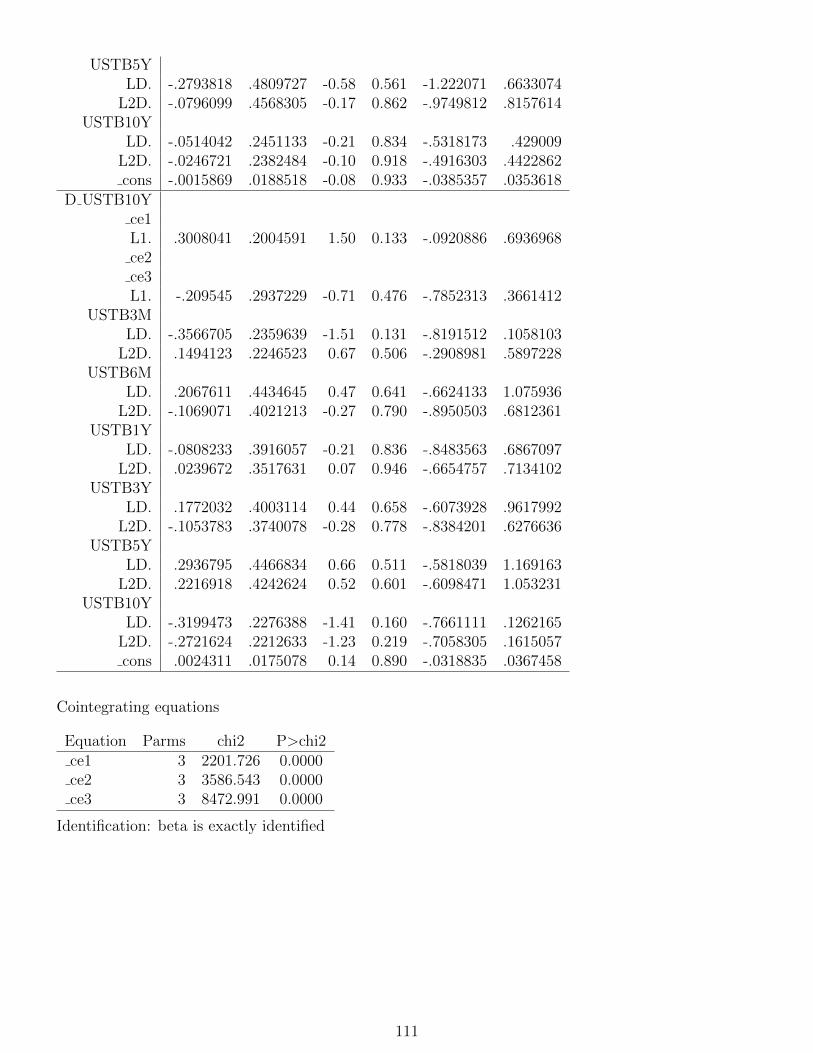
USTB5YLD. -.2793818 .4809727 -0.58 0.561 -1.222071 .6633074

L2D. -.0796099 .4568305 -0.17 0.862 -.9749812 .8157614USTB10Y

LD. -.0514042 .2451133 -0.21 0.834 -.5318173 .429009L2D. -.0246721 .2382484 -0.10 0.918 -.4916303 .4422862cons -.0015869 .0188518 -0.08 0.933 -.0385357 .0353618

D USTB10Yce1L1. .3008041 .2004591 1.50 0.133 -.0920886 .6936968ce2ce3L1. -.209545 .2937229 -0.71 0.476 -.7852313 .3661412

USTB3MLD. -.3566705 .2359639 -1.51 0.131 -.8191512 .1058103

L2D. .1494123 .2246523 0.67 0.506 -.2908981 .5897228USTB6M

LD. .2067611 .4434645 0.47 0.641 -.6624133 1.075936L2D. -.1069071 .4021213 -0.27 0.790 -.8950503 .6812361

USTB1YLD. -.0808233 .3916057 -0.21 0.836 -.8483563 .6867097

L2D. .0239672 .3517631 0.07 0.946 -.6654757 .7134102USTB3Y

LD. .1772032 .4003114 0.44 0.658 -.6073928 .9617992L2D. -.1053783 .3740078 -0.28 0.778 -.8384201 .6276636

USTB5YLD. .2936795 .4466834 0.66 0.511 -.5818039 1.169163

L2D. .2216918 .4242624 0.52 0.601 -.6098471 1.053231USTB10Y

LD. -.3199473 .2276388 -1.41 0.160 -.7661111 .1262165L2D. -.2721624 .2212633 -1.23 0.219 -.7058305 .1615057cons .0024311 .0175078 0.14 0.890 -.0318835 .0367458

Cointegrating equations

Equation Parms chi2 P>chi2ce1 3 2201.726 0.0000ce2 3 3586.543 0.0000ce3 3 8472.991 0.0000

Identification: beta is exactly identified

111

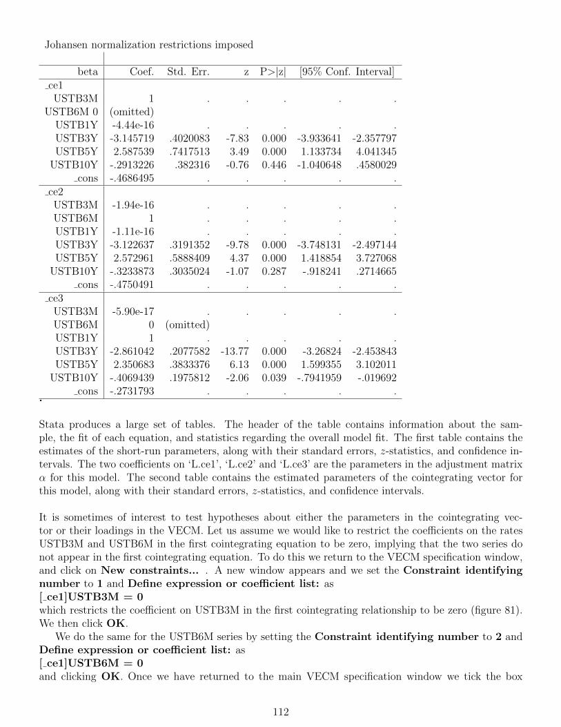
Johansen normalization restrictions imposed

beta Coef. Std. Err. z P>|z| [95% Conf. Interval]ce1USTB3M 1 . . . . .

USTB6M 0 (omitted)USTB1Y -4.44e-16 . . . . .USTB3Y -3.145719 .4020083 -7.83 0.000 -3.933641 -2.357797USTB5Y 2.587539 .7417513 3.49 0.000 1.133734 4.041345

USTB10Y -.2913226 .382316 -0.76 0.446 -1.040648 .4580029cons -.4686495 . . . . .

ce2USTB3M -1.94e-16 . . . . .USTB6M 1 . . . . .USTB1Y -1.11e-16 . . . . .USTB3Y -3.122637 .3191352 -9.78 0.000 -3.748131 -2.497144USTB5Y 2.572961 .5888409 4.37 0.000 1.418854 3.727068

USTB10Y -.3233873 .3035024 -1.07 0.287 -.918241 .2714665cons -.4750491 . . . . .

ce3USTB3M -5.90e-17 . . . . .USTB6M 0 (omitted)USTB1Y 1 . . . . .USTB3Y -2.861042 .2077582 -13.77 0.000 -3.26824 -2.453843USTB5Y 2.350683 .3833376 6.13 0.000 1.599355 3.102011

USTB10Y -.4069439 .1975812 -2.06 0.039 -.7941959 -.019692cons -.2731793 . . . . .

.

Stata produces a large set of tables. The header of the table contains information about the sam-ple, the fit of each equation, and statistics regarding the overall model fit. The first table contains theestimates of the short-run parameters, along with their standard errors, z-statistics, and confidence in-tervals. The two coefficients on ‘L.ce1’, ‘L.ce2’ and ‘L.ce3’ are the parameters in the adjustment matrixα for this model. The second table contains the estimated parameters of the cointegrating vector forthis model, along with their standard errors, z-statistics, and confidence intervals.

It is sometimes of interest to test hypotheses about either the parameters in the cointegrating vec-tor or their loadings in the VECM. Let us assume we would like to restrict the coefficients on the ratesUSTB3M and USTB6M in the first cointegrating equation to be zero, implying that the two series donot appear in the first cointegrating equation. To do this we return to the VECM specification window,and click on New constraints... . A new window appears and we set the Constraint identifyingnumber to 1 and Define expression or coefficient list: as[ ce1]USTB3M = 0which restricts the coefficient on USTB3M in the first cointegrating relationship to be zero (figure 81).We then click OK.

We do the same for the USTB6M series by setting the Constraint identifying number to 2 andDefine expression or coefficient list: as[ ce1]USTB6M = 0and clicking OK. Once we have returned to the main VECM specification window we tick the box

112

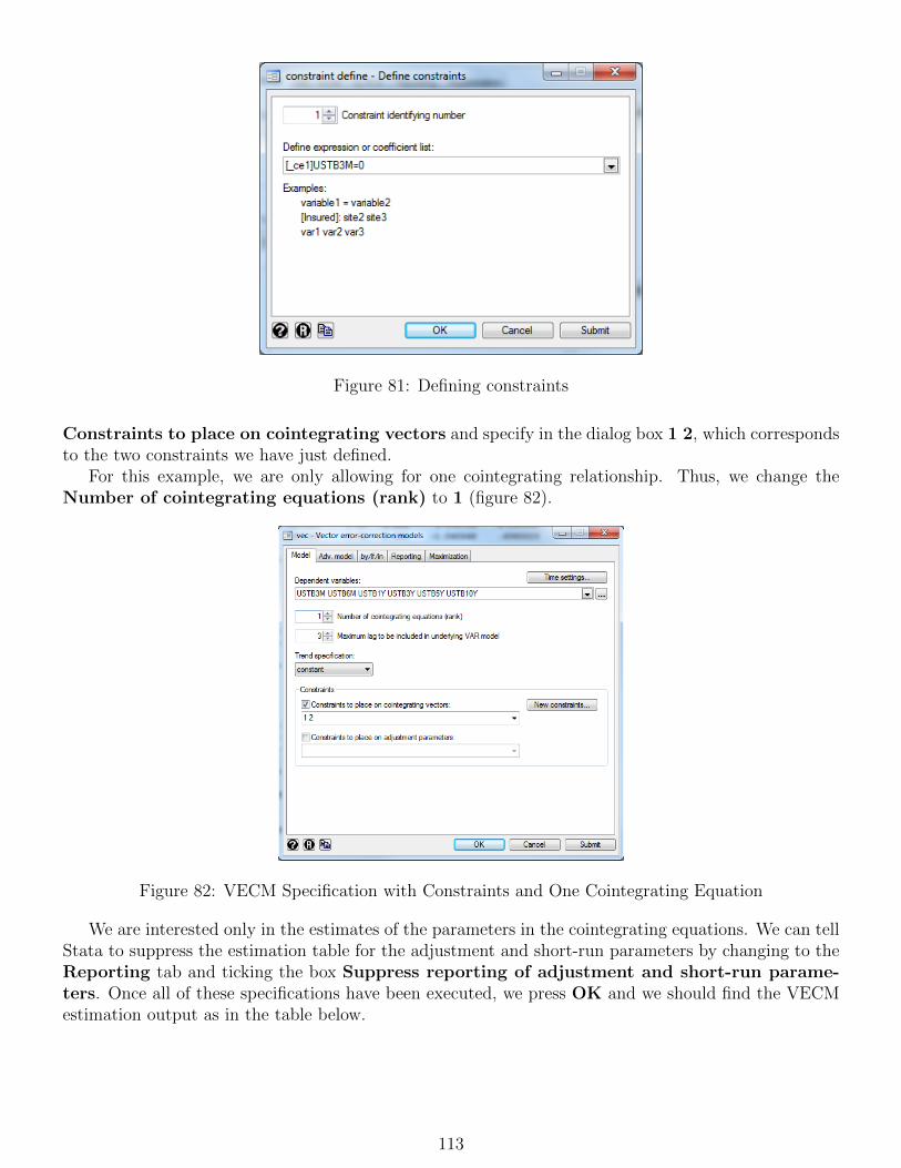
Figure 81: Defining constraints

Constraints to place on cointegrating vectors and specify in the dialog box 1 2, which correspondsto the two constraints we have just defined.

For this example, we are only allowing for one cointegrating relationship. Thus, we change theNumber of cointegrating equations (rank) to 1 (figure 82).

Figure 82: VECM Specification with Constraints and One Cointegrating Equation

We are interested only in the estimates of the parameters in the cointegrating equations. We can tellStata to suppress the estimation table for the adjustment and short-run parameters by changing to theReporting tab and ticking the box Suppress reporting of adjustment and short-run parame-ters. Once all of these specifications have been executed, we press OK and we should find the VECMestimation output as in the table below.

113

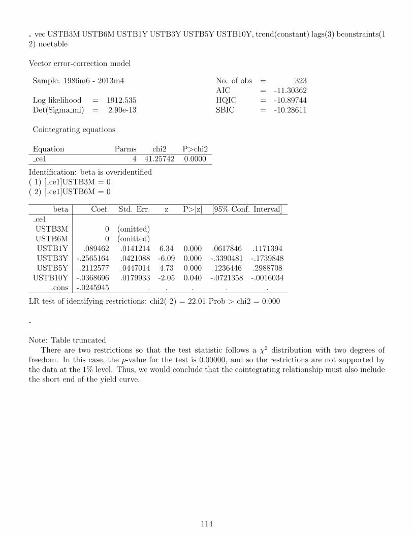
. vec USTB3M USTB6M USTB1Y USTB3Y USTB5Y USTB10Y, trend(constant) lags(3) bconstraints(12) noetable

Vector error-correction model

Sample: 1986m6 - 2013m4 No. of obs = 323AIC = -11.30362

Log likelihood = 1912.535 HQIC = -10.89744Det(Sigma ml) = 2.90e-13 SBIC = -10.28611

Cointegrating equations

Equation Parms chi2 P>chi2ce1 4 41.25742 0.0000

Identification: beta is overidentified( 1) [ ce1]USTB3M = 0( 2) [ ce1]USTB6M = 0

beta Coef. Std. Err. z P>|z| [95% Conf. Interval]ce1USTB3M 0 (omitted)USTB6M 0 (omitted)USTB1Y .089462 .0141214 6.34 0.000 .0617846 .1171394USTB3Y -.2565164 .0421088 -6.09 0.000 -.3390481 -.1739848USTB5Y .2112577 .0447014 4.73 0.000 .1236446 .2988708

USTB10Y -.0368696 .0179933 -2.05 0.040 -.0721358 -.0016034cons -.0245945 . . . . .

LR test of identifying restrictions: chi2( 2) = 22.01 Prob > chi2 = 0.000

.

Note: Table truncatedThere are two restrictions so that the test statistic follows a χ2 distribution with two degrees of

freedom. In this case, the p-value for the test is 0.00000, and so the restrictions are not supported bythe data at the 1% level. Thus, we would conclude that the cointegrating relationship must also includethe short end of the yield curve.

114

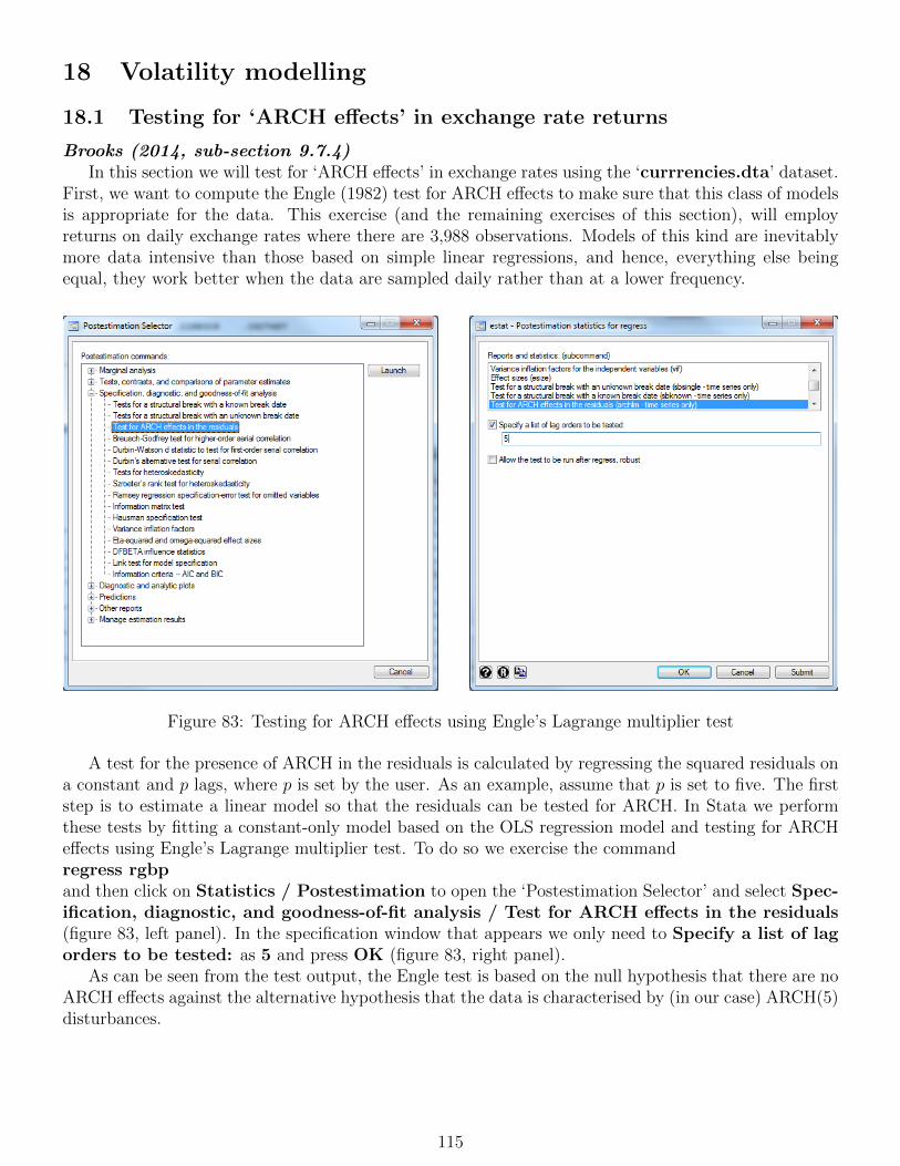
18 Volatility modelling

18.1 Testing for ‘ARCH effects’ in exchange rate returns

Brooks (2014, sub-section 9.7.4)In this section we will test for ‘ARCH effects’ in exchange rates using the ‘currrencies.dta’ dataset.

First, we want to compute the Engle (1982) test for ARCH effects to make sure that this class of modelsis appropriate for the data. This exercise (and the remaining exercises of this section), will employreturns on daily exchange rates where there are 3,988 observations. Models of this kind are inevitablymore data intensive than those based on simple linear regressions, and hence, everything else beingequal, they work better when the data are sampled daily rather than at a lower frequency.

Figure 83: Testing for ARCH effects using Engle’s Lagrange multiplier test

A test for the presence of ARCH in the residuals is calculated by regressing the squared residuals ona constant and p lags, where p is set by the user. As an example, assume that p is set to five. The firststep is to estimate a linear model so that the residuals can be tested for ARCH. In Stata we performthese tests by fitting a constant-only model based on the OLS regression model and testing for ARCHeffects using Engle’s Lagrange multiplier test. To do so we exercise the commandregress rgbpand then click on Statistics / Postestimation to open the ‘Postestimation Selector’ and select Spec-ification, diagnostic, and goodness-of-fit analysis / Test for ARCH effects in the residuals(figure 83, left panel). In the specification window that appears we only need to Specify a list of lagorders to be tested: as 5 and press OK (figure 83, right panel).

As can be seen from the test output, the Engle test is based on the null hypothesis that there are noARCH effects against the alternative hypothesis that the data is characterised by (in our case) ARCH(5)disturbances.

115

. estat archlm, lags(5)

LM test for autoregressive conditional heteroskedasticity (ARCH)lags(p) chi2 df Prob > chi2

5 301.697 5 0.0000H0: no ARCH effects vs. H1: ARCH(p) disturbances

.

The test shows a p-value of 0.0000, which is well below 0.05, suggesting the presence of ARCH effectsin the pound-dollar returns.

18.2 Estimating GARCH models

Brooks (2014, section 9.9)To estimate a GARCH-type model in Stata, we select Statistics / Time series / ARCH/GARCH

/ ARCH and GARCH models. In the ARCH specification window that appears we define Depen-dent variable: rjpy (figure 84, top panel). We do not include any further independent variables butinstead continue by specifying the Main model specification. Let us first Specify maximum lagswith respect to the ARCH and GARCH terms. The default is to estimate the model with one ARCHand no GARCH. In our example we want to include one ARCH and one GARCH term (i.e. one lag ofthe squared errors and one lag of the conditional variance, respectively). Thus, we input 1 GARCHmaximum lag. If we wanted to include a list of non-consecutive lags, e.g. lag 1 and lag 3, we could dothis by selecting Supply list of lags and then specifying the specific lags we want to include for theARCH and GARCH.

The ARCH specification window provides various options of how to vary the model (figure 84, lowerpanel). You can have a look at the options by clicking through the various tabs. Model 2 can be usedto include ARCH-M terms (see later in this section), while Model 3 provides different options for theassumed distribution of the errors, e.g. instead of assuming a Gaussian distribution we can specify aStudent’s t-distribution. In the final, tab we can specify the Maximization technique. Log-likelihoodfunctions for ARCH models are often not well behaved so that convergence may not be achieved with thedefault estimation settings. It is possible in Stata to select the iterative algorithm (Newton-Raphson,BHHH, BFGS, DFP), to change starting values, to increase the maximum number of iterations or toadjust the convergence criteria. For example, if convergence is not achieved, or implausible parameterestimates are obtained, it is sensible to re-do the estimation using a different set of starting values and/ora different optimisation algorithm.

Estimating the GARCH(1,1) model for the yen-dollar (‘rjpy’) series using the instructions as listedabove, and the default settings elsewhere would yield the table of results after the figures.

116

Figure 84: Specifying a GARCH(1,1) Model

117

. arch rjpy, arch(1/1) garch(1/1)

(setting optimization to BHHH)Iteration 0: log likelihood = -2530.6526Iteration 1: log likelihood = -2517.2661Iteration 2: log likelihood = -2498.6104Iteration 3: log likelihood = -2474.2445Iteration 4: log likelihood = -2466.0788(switching optimization to BFGS)Iteration 5: log likelihood = -2462.2839Iteration 6: log likelihood = -2461.2981Iteration 7: log likelihood = -2461.0456Iteration 8: log likelihood = -2460.998Iteration 9: log likelihood = -2460.989Iteration 10: log likelihood = -2460.9862Iteration 11: log likelihood = -2460.9861Iteration 12: log likelihood = -2460.9861

ARCH family regression

Sample: 08jul2002 - 06jun2013 Number of obs = 3,987Distribution: Gaussian Wald chi2(.) = .Log likelihood = -2460.986 Prob > chi2 = .

OPGrjpy Coef. Std. Err. z P>|z| [95% Conf. Interval]

rjpycons .0025464 .0065108 0.39 0.696 -.0102146 .0153073

ARCHarchL1. .0475988 .0035622 13.36 0.000 .0406171 .0545805

garchL1. .9325011 .0052088 179.02 0.000 .922292 .9427101

cons .0044893 .000466 9.63 0.000 .003576 .0054025

.

The coefficients on both the lagged squared residuals and lagged conditional variance terms in theconditional variance equation (i.e. the third panel in the output subtitled ‘ARCH’) are highly statisticallysignificant. Also, as is typical of GARCH model estimates for financial asset returns data, the sumof the coefficients on the lagged squared error and lagged conditional variance is very close to unity(approximately 0.98). This implies that shocks to the conditional variance will be highly persistent.This can be seen by considering the equations for forecasting future values of the conditional varianceusing a GARCH model given in a subsequent section. A large sum of these coefficients will imply thata large positive or a large negative return will lead future forecasts of the variance to be high for aprotracted period. The individual conditional variance coefficients are also as one would expect. Thevariance intercept term cons in the ‘ARCH’ panel is very small, and the ‘ARCH’-parameter ‘L1.arch’

118

is around 0.05 while the coefficient on the lagged conditional variance ‘L1.garch’ is larger at 0.93.Stata allows for a series of postestimation commands. The following list provides a brief overview

of these commands. Details can be obtained in the Stata User Manuel under the entry [TS] archpostestimation:

• estat

AIC, BIC, VCE, and estimation sample summary

• estimates

cataloging estimation results

• lincom

point estimates, standard errors, testing, and inference for linear combinations of coefficients

• lrtest

likelihood-ratio test

• margins

marginal means, predictive margins, marginal effects, and average marginal effects

• marginsplot

graph the results from margins (profile plots, interaction plots, etc.)

• nlcom

point estimates, standard errors, testing, and inference for nonlinear combinations of coefficients

• predict

predictions, residuals, influence statistics, and other diagnostic measures

• predictnl

point estimates, standard errors, testing, and inference for generalized predictions

• test

Wald tests of simple and composite linear hypotheses

• testnl

Wald tests of nonlinear hypotheses

18.3 GJR and EGARCH models

Brooks (2014, section 9.14)Since the GARCH model was developed, numerous extensions and variants have been proposed. In

this section we will estimate two of them in Stata, the GJR and EGARCH models. The GJR modelis a simple extension of the GARCH model with an additional term added to account for possibleasymmetries. The exponential GARCH (EGARCH) model extends the classical GARCH by correctingthe non-negativity constraint and by allowing for asymmetries.

We start by estimating the EGARCH model. We select Statistics / Time series / ARCH/GARCH.We see that there are a number of variants on the standard ARCH and GARCH model available. Fromthe list we select Nelson’s EGARCH model. The arch specification window appears and we notice

119

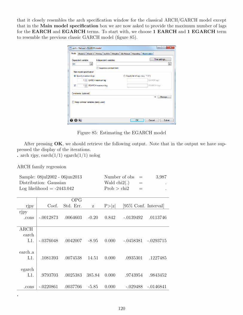
that it closely resembles the arch specification window for the classical ARCH/GARCH model exceptthat in the Main model specification box we are now asked to provide the maximum number of lagsfor the EARCH and EGARCH terms. To start with, we choose 1 EARCH and 1 EGARCH termto resemble the previous classic GARCH model (figure 85).

Figure 85: Estimating the EGARCH model

After pressing OK, we should retrieve the following output. Note that in the output we have sup-pressed the display of the iterations.. arch rjpy, earch(1/1) egarch(1/1) nolog

ARCH family regression

Sample: 08jul2002 - 06jun2013 Number of obs = 3,987Distribution: Gaussian Wald chi2(.) = .Log likelihood = -2443.042 Prob > chi2 = .

OPGrjpy Coef. Std. Err. z P>|z| [95% Conf. Interval]

rjpycons -.0012873 .0064603 -0.20 0.842 -.0139492 .0113746

ARCHearch

L1. -.0376048 .0042007 -8.95 0.000 -.0458381 -.0293715

earch aL1. .1081393 .0074538 14.51 0.000 .0935301 .1227485

egarchL1. .9793703 .0025383 385.84 0.000 .9743954 .9843452

cons -.0220861 .0037766 -5.85 0.000 -.029488 -.0146841

.

120

Looking at the results, we find that all EARCH and EGARCH terms are statistically significant.The EARCH terms represent the influence of news – lagged innovations – in Nelsons (1991) EGARCHmodel. The first term ‘L1.earch’ captures the

υt−1√σ2t−1

term and ‘L1.earch a’ captures the

|υt−1|√σ2t−1

−√

2

π

term. The negative estimate on the ‘L1.earch’ term implies that negative shocks result in a lowernext period conditional variance than positive shocks of the same sign. The result for the EGARCHasymmetry term is the opposite to what would have been expected in the case of the application of aGARCH model to a set of stock returns. But arguably, neither the leverage effect or volatility effectexplanations for asymmetries in the context of stocks apply here. For a positive return shock, theresults suggest more yen per dollar and therefore a strengthening dollar and a weakening yen. Thus,the EGARCH results suggest that a strengthening dollar (weakening yen) leads to higher next periodvolatility than when the yen strengthens by the same amount.

Let us now test a GJR model. For this we click on Statistics / Time series / ARCH/GARCHand select GJR form of threshold ARCH model. In the GJR specification window that appears,we specify 1 ARCH maximum lag, 1 TARCH maximum lag and 1 GARCH maximum lag(figure 86), and press OK to fit the model.

Figure 86: Estimation the GJR model

The following GJR estimation output should appear. Note that the display of iterations is againsuppressed.

121

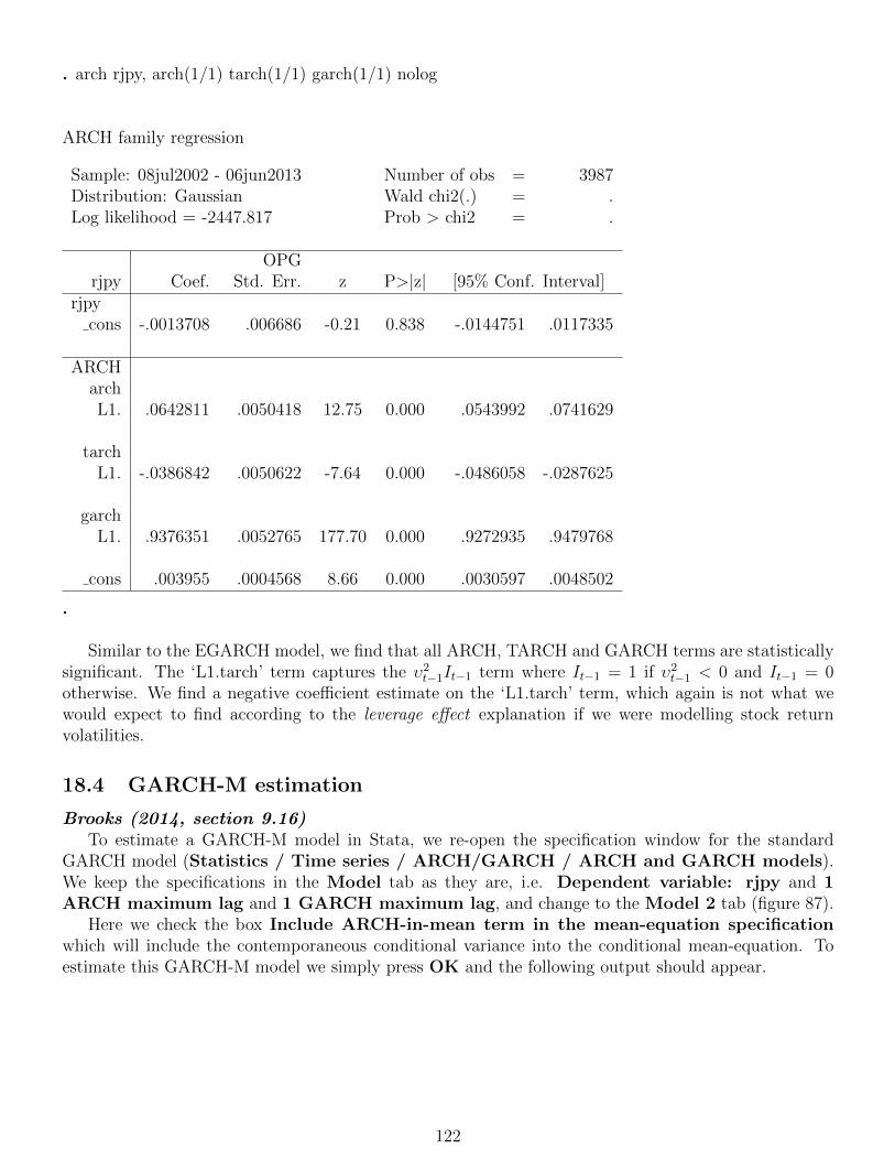
. arch rjpy, arch(1/1) tarch(1/1) garch(1/1) nolog

ARCH family regression

Sample: 08jul2002 - 06jun2013 Number of obs = 3987Distribution: Gaussian Wald chi2(.) = .Log likelihood = -2447.817 Prob > chi2 = .

OPGrjpy Coef. Std. Err. z P>|z| [95% Conf. Interval]

rjpycons -.0013708 .006686 -0.21 0.838 -.0144751 .0117335

ARCHarchL1. .0642811 .0050418 12.75 0.000 .0543992 .0741629

tarchL1. -.0386842 .0050622 -7.64 0.000 -.0486058 -.0287625

garchL1. .9376351 .0052765 177.70 0.000 .9272935 .9479768

cons .003955 .0004568 8.66 0.000 .0030597 .0048502

.

Similar to the EGARCH model, we find that all ARCH, TARCH and GARCH terms are statisticallysignificant. The ‘L1.tarch’ term captures the υ2t−1It−1 term where It−1 = 1 if υ2t−1 < 0 and It−1 = 0otherwise. We find a negative coefficient estimate on the ‘L1.tarch’ term, which again is not what wewould expect to find according to the leverage effect explanation if we were modelling stock returnvolatilities.

18.4 GARCH-M estimation

Brooks (2014, section 9.16)To estimate a GARCH-M model in Stata, we re-open the specification window for the standard

GARCH model (Statistics / Time series / ARCH/GARCH / ARCH and GARCH models).We keep the specifications in the Model tab as they are, i.e. Dependent variable: rjpy and 1ARCH maximum lag and 1 GARCH maximum lag, and change to the Model 2 tab (figure 87).

Here we check the box Include ARCH-in-mean term in the mean-equation specificationwhich will include the contemporaneous conditional variance into the conditional mean-equation. Toestimate this GARCH-M model we simply press OK and the following output should appear.

122

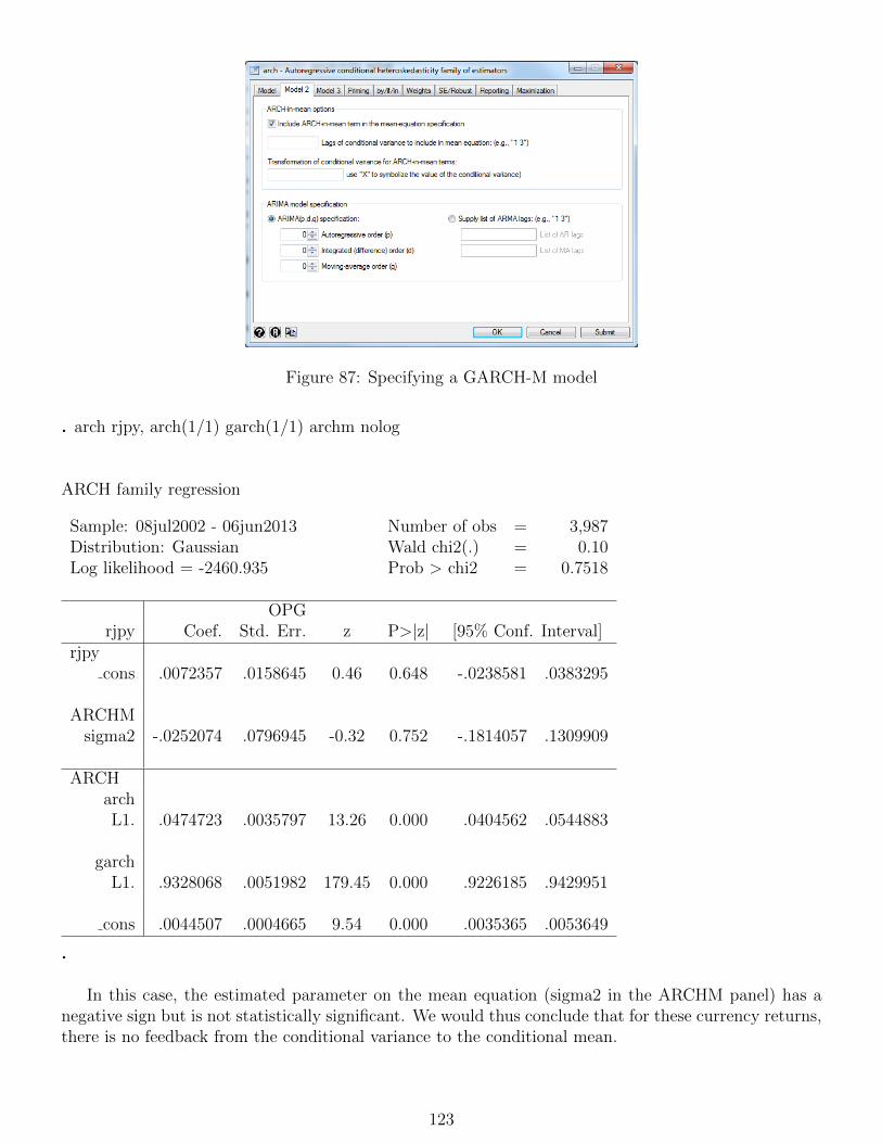
Figure 87: Specifying a GARCH-M model

. arch rjpy, arch(1/1) garch(1/1) archm nolog

ARCH family regression

Sample: 08jul2002 - 06jun2013 Number of obs = 3,987Distribution: Gaussian Wald chi2(.) = 0.10Log likelihood = -2460.935 Prob > chi2 = 0.7518

OPGrjpy Coef. Std. Err. z P>|z| [95% Conf. Interval]

rjpycons .0072357 .0158645 0.46 0.648 -.0238581 .0383295

ARCHMsigma2 -.0252074 .0796945 -0.32 0.752 -.1814057 .1309909

ARCHarchL1. .0474723 .0035797 13.26 0.000 .0404562 .0544883

garchL1. .9328068 .0051982 179.45 0.000 .9226185 .9429951

cons .0044507 .0004665 9.54 0.000 .0035365 .0053649

.

In this case, the estimated parameter on the mean equation (sigma2 in the ARCHM panel) has anegative sign but is not statistically significant. We would thus conclude that for these currency returns,there is no feedback from the conditional variance to the conditional mean.

123

18.5 Forecasting from GARCH models

Brooks (2014, section 9.17)GARCH-type models can be used to forecast volatility. In this sub-section, we will focus on generat-

ing the conditional variance forecasts using Stata. Let us assume we want to generate forecasts based onthe EGARCH model estimated earlier for the forecast period 06Jul2011 to 06Jun2013. The first step isto re-estimate the EGARCH model for the sub-sample running until 05Jul2011. To estimate the modelwe click on Statistics / Time series / ARCH/GARCH / Nelson’s EGARCH and we inputthe same specifications as previously, i.e. Dependent variable: rjpy, 1 EARCH maximum lag, 1EGARCH maximum lag (see figure 85 above). However, now we only want to estimate the modelfor a sub-period of the data so we change to the by/if/in tab and define the following time restrictionin the If: (expression) dialogue box:Date<=td(06jul2011)Then we press OK to fit the model.

Next, we generate the conditional variance forecasts. We select Predictions / Means from dif-ferenced or undifferenced series, conditional variances, residuals, etc. in the ‘PostestimationSelector’ and are now presented with the ‘predict’ specification window (figure 88).

Figure 88: Generating Static Forecasts of the Conditional Variance

There is a variety of predicted values we can produce, which are listed under the Produce: headline.As we want to generate forecasts of the conditional variance we select the third option from the topwhich is Values for the conditional variance (figure 89, left panel). As was the case for the previousforecast exercise, we can either create static (a series of rolling single-step-ahead) forecasts or dynamic(multiple-step-ahead) forecasts. Let us start with the static forecasts. We change to the Optionstab and make sure that the option One-step prediction is selected. However, as this is the defaultspecification we do not need to make any changes. Finally we have to give the new series a name. Wereturn to the Main tab and specify New variable name: cvar rjpy stat. Then we press OK.

Next we generate the dynamic conditional variance forecasts. We re-open the ‘predict’ specificationwindow and change the name of the new variable to cvar rjpy dyn. We check that the Produceoption Values for the conditional variance is selected and change to the Options tab. We nowselect Switch to dynamic predictions at time and enter the following starting value into the dialoguebox:td(06jul2011)

124

Figure 89: Generating Dynamic Forecasts of the Conditional Variances

which represents the start of the forecast period (figure 89, right panel). Once all the changes have beenmade we click on OK and the new series should appear in the Variables window.

Finally we want to graphically examine the conditional variance forecasts. To generate a time seriesgraph of the static and dynamic forecasts we click on Graphics / Time series graphs / Lineplots. We create Plot 1 which contains the series cvar rjpy stat and Plot 2 comprising the seriescvar rjpy dyn. As we only want to see the values for the forecast period we change to the if/in taband specify If: Date>=td(06jul2011). By clicking OK, the following graph should appear (figure90).

Figure 90: Graph of the Static and Dynamic Forecasts of the Conditional Variance

What do we observe? For the dynamic forecasts (red line), the value of the conditional variancestarts from a historically low level at the end of the estimation period, relative to its unconditionalaverage. Therefore the forecasts converge upon their long-term mean value from below as the forecasthorizon increases. Turning to the static forecasts (blue line), it is evident that the variance forecastshave one large spike in mid-2011 and another large spike in late 2011. After a period of relatively high

125

conditional variances in the first half of 2012, the variances stabilise and enter a phase of historicallyquite low variance in the second half of 2012. 2013 sees a large rise in conditional variances and theyremain at a relatively high level for the rest of the sample period. Since in the case of the static forecastswe are looking at a series of rolling one-step ahead forecasts for the conditional variance, the values showmuch more volatility than those for the dynamic forecasts. Note that while the forecasts are updateddaily based on new information that feeds into the forecasts, the parameter estimates themselves are notupdated. Thus, towards the end of the sample, the forecasts are based on estimates almost two yearsold. If we wanted to update the model estimates as we rolled through the sample, we would need towrite some code to do this within a loop - it would also run much more slowly as we would be estimatinga lot of GARCH models rather than one.

Predictions can be similarly produced for any member of the GARCH family that is estimable withthe software. For specifics on how to generate predictions after specific GARCH or ARCH models,please refer to the corresponding postestimation commands section in the Stata manual.

18.6 Estimation of multivariate GARCH models

Brooks (2014, section 9.30)Multivariate GARCH models are in spirit very similar to their univariate counterparts, except that

the former also specify equations for how the covariances move over time and are therefore by their natureinherently more complex to specify and estimate. To estimate a multivariate GARCH model in Stata,we click on Statistics / Multivariate Time series and we select Multivariate GARCH. In the‘mgarch’ specification window, we are first asked to select the type of multivariate GARCH model that wewould like to estimate. Stata allows us to esimtate four commonly used parameterizations: the diagonalvech model, the constant conditional correlation model, the dynamic conditional correlation model, andthe time-varying conditional correlation model. We select the Constant conditional correlation(ccc) model for now (figure 91, left panel).54 Next we need to specify the variance equation by clickingon Create... next to the Equations dialogue box. A new window appears (figure 91, right panel).We specify the three currency returns series in the Dependent variables box. Additional exogenousvariables can be incorporated into the variance equation but for now we just leave the settings as theyare and press OK to return to the main specification window. Next we define the maximum lags of theARCH and GARCH terms. We select 1 ARCH maximum lag and 1 GARCH maximum lag.

By default, Stata estimates the parameters of MGARCH models by maximum likelihood (ML), as-suming that the errors come from a multivariate normal distribution. However, Stata also allows toassume a multivariate Student’s t distribution for the error terms. However, we will keep the Gaussiannormal distribution for now. Alternatively, there are various other options to change the model spec-ification, e.g. defining constraints on parameters, adjusting the standard errors or the maximisationprocedure. However, for now, we will keep the default settings. The complexity of this model meansthat it takes longer to estimate than any of the univariate GARCH or other models examined previously.Thus, it might make sense to suppress the Iterations log under the Maximization tab. In orderto estimate the model, we press OK. The model output shall resemble the table below after the figures(note that the iteration log is not shown).

The table is separated into different parts. The header provides details on the estimation sampleand reports a Wald test against the null hypothesis that all the coefficients on the independent variablesin the mean equations are zero, which in our case is only the constant. The null hypothesis is rejectedat the 5% level. The output table is organised by dependent variable. For each dependent variable, we

54The Diagonal vech model (dvech) does not converge and, thus, does not produce any estimates given the data athand and the specification that we want to estimate. Therefore, we use the Constant conditional correlation model in thefollowing application. However, a corresponding Diagonal vech model would theoretically be estimated in the same wayand only the model type in the bottom left corner needs to be adjusted.

126

Figure 91: Specifying a Multivariate GARCH model

first find the estimates for the conditional mean equation, followed by the conditional variance estimatesin a separate panel. It is evident that the parameter estimates are all both plausible and statisticallysignificant. In the final panels Stata reports results for the conditional correlation parameters. Forexample, the conditional correlation between the standardized residuals for ‘reur’ and ‘rgbp’ is estimatedto be 0.68.

127

. mgarch ccc (reur rgbp rjpy =), arch(1/1) garch(1/1) nologConstant conditional correlation MGARCH modelSample: 07jul2002 - 06jun2013 Number of obs = 3,987Distribution: Gaussian Wald chi2(.) = .Log likelihood = -5276.172 Prob > chi2 = .

rjpy Coef. Std. Err. z P>|z| [95% Conf. Interval]reur

cons -.0177595 .0062647 -2.83 0.005 -.0300381 -.0054809ARCH reur

archL1. .0272742 .0026931 10.13 0.000 .0219959 .0325525

garchL1. .97016 .0027863 348.19 0.000 .964699 .975621

cons .0005909 .0001805 3.27 0.001 .000237 .0009447

rgbpcons -.0090884 .005636 -1.61 0.107 -.0201347 .0019578

ARCH rgbparchL1. .0312925 .0033888 9.23 0.000 .0246506 .0379343

garchL1. .96503 .0036734 262.71 0.000 .9578303 .9722297

cons .0006731 .0001945 3.46 0.001 .000292 .0010542

rjpycons .0009727 .0067046 0.15 0.885 -.0121682 .0141135

ARCH rjpyarchL1. .0572256 .0074223 7.71 0.000 .0426782 .071773

garchL1. .9190881 .0102905 89.31 0.000 .8989191 .9392571

cons .0054909 .0010407 5.28 0.000 .0034511 .0075307

Correlationreur

rgbp .6972162 .0081495 85.55 0.000 .6812436 .7131889rjpy .3126349 .0143502 21.79 0.000 .2845089 .3407608

rgbprjpy .2287797 .0150679 15.18 0.000 .1992471 .258312

.

128

19 Modelling seasonality in financial data

19.1 Dummy variables for seasonality

Brooks (2014, sub-section 10.3.2)In this sub-section, we will test for the existence of a January effect in the stock returns of Microsoft

using the ‘macro.dta’ workfile. In order to examine whether there is indeed a January effect in amonthly time series regression, a dummy variable is created that takes the value 1 only in the monthsof January. To create the dummy JANDUM it is easiest to first create a new variable that extractsthe month from the Date series. To do so, we type the following command into the Command windowand press Enter:generate Month=month(dofm(Date))where month() tells Stata to extract the month component from the ‘Date’ series and the ‘dofm()’ termis needed as the ‘month()’ command can only be performed on date series that are coded as daily data.If you inspect the new series in the Data Editor you will notice that the series Month contains a ‘1’ ifthe month is January, a ‘2’ if the month is February, a ‘3’ if the month is March, etc. Now it is verysimple to create the ‘JANDUM’ dummy. We type in the command window the following expression:generate JANDUM = 1 if Month==1

and we press Enter. The new variable ‘JANDUM’ contains a ‘.’ for all months except January (forwhich it takes the value 1). If we want to replace the ‘.’ with zeros we can use the following Statacommand:replace JANDUM = 0 if JANDUM==.

We can now run the APT-style regression first used in section 7 but this time including the new‘JANDUM’ dummy variable. The command for this regressions is as follows:regress ermsoft ersandp dprod dcredit dinflation dmoney dspread rterm FEB98DUMFEB03DUM JANDUMThe results of this regression are presented below.

129

. regress ermsoft ersandp dprod dcredit dinflation dmoney dspread rterm FEB98DUM FEB03DUMJANDUM

Source SS df MS Number of obs = 324F( 10, 313) = 16.89

Model 22373.2276 10 2237.32276 Prob > F = 0.0000Residual 41466.8627 313 132.48199 R-squared = 0.3505

Adj R-squared = 0.3297Total 63840.0903 323 197.647338 Root MSE = 11.51

Coef. Std. Err. t P>|t| [95% Conf. Interval]

ersandp 1.386384 .1432828 9.68 0.000 1.104465 1.668303dprod -1.242103 1.206216 -1.03 0.304 -3.61542 1.131213

dcredit -.0000318 .0000697 -0.46 0.648 -.0001689 .0001053dinflation 1.96292 2.242415 0.88 0.382 -2.449192 6.375033

dmoney -.0037369 .0343982 -0.11 0.914 -.0714178 .063944dspread 4.281578 6.333687 0.68 0.500 -8.180408 16.74356

rterm 4.62212 2.287478 2.02 0.044 .1213431 9.122897FEB98DUM -65.65307 11.59806 -5.66 0.000 -88.47309 -42.83305FEB03DUM -66.8003 11.57405 -5.77 0.000 -89.57308 -44.02753

JANDUM 4.127243 2.834769 1.46 0.146 -1.45037 9.704855cons -.2229397 .8979781 -0.25 0.804 -1.989776 1.543897

.

As can be seen, the dummy is just outside being statistically significant at the 10% level, and ithas the expected positive sign. The coefficient value of 4.127, suggests that on average and holdingeverything else equal, Microsoft stock returns are around 4% higher in January than the average forother months of the year.

19.2 Estimating Markov switching models

Brooks (2014, sections 10.5–10.8)In this sub-section, we will be estimating a Markov switching model in Stata. The example that

we will consider in this sub-section relates to the changes in house prices series used previously. So were-open ukhp.dta. Stata enables us to fit two types of Markov switching models: Markov switchingdynamic regression (MSDR) models which allow a quick adjustment after the process changes stateand Markov switching autoregression (MSAR) models that allow a more gradual adjustment. In thisexample we will focus on the former case.

To open the specification window for Markov switching regressions, we select Statistics / Timeseries / Markov-switching model. In the specification window we first select the Model. As wewant to test a Dynamic regression we just keep the default option. Next we are asked to select theDependent variable and we select dhp. We want to estimate a simple switching model with just avarying intercept in each state. As Stata automatically includes the (state-dependent) intercept we donot need to specify any further variables in the boxes for the ‘Nonswitch variables’ or the variables with‘Switching coefficients’. However, if we wanted to include further variables that allow for either changingor non-changing coefficient parameters across states we could do this using the respective dialogue boxes.Let us move on to specifying the Number of states. The default is 2 states and, for now, we stickwith the default option. Finally, we also want the variance parameters to vary across states, so we check

130

the box Specify state-dependent variance paramters. Once all of these specifications are made,the window shall resemble figure 92.

Figure 92: Specifying a Markov switching model

We click OK and the results shall appear as in the following table. Examining the results, it isclear that the model has successfully captured the features of the data. Two distinct regimes have beenidentified: regime 1 with a negative mean return (corresponding to a price fall of 0.20% per month) anda relatively high volatility, whereas regime 2 has a high average price increase of 0.96% per month anda much lower standard deviation.

131

. mswitch dr dhp, varswitch

Performing EM optimization:

Performing gradient-based optimization:

Iteration 0: log likelihood = -406.77203Iteration 1: log likelihood = -405.59694Iteration 2: log likelihood = -404.50815Iteration 3: log likelihood = -404.39043Iteration 4: log likelihood = -404.3894Iteration 5: log likelihood = -404.3894

Markov-switching dynamic regression

Sample: 1991m2 - 2013m5 No. of obs = 268Number of states = 2 AIC = 3.0626Unconditional probabilities: transition HQIC = 3.0949

SBIC = 3.1430Log likelihood = -404.3894

dhp Coef. Std. Err. z P>|z| [95% Conf. Interval]State1

cons -.20468 .1352158 -1.51 0.130 -.4696982 .0603382State2

cons .9588438 .1080784 8.87 0.000 .747014 1.170674sigma1 1.174341 .0880885 1.013783 1.360328sigma2 .9358422 .0581499 .8285371 1.057044

p11 .9714903 .0242549 .8596267 .9947537p21 .0248452 .0193783 .005285 .1088752

.

To see the transition probabilities matrix, we open the ‘Postestimation Selector’ (Statistics /Postestimation) and then select Specification, diagnostic, and goodness-of-fit analysis / Tableof transition probabilities (figure 93, left panel).

Clicking on Launch, the specification window as shown in figure 93, right panel, appears and wesimply click OK to generate the following trasition matrix. Looking at the results, it appears that theregimes are fairly stable, with probabilities of around 97% of remaining in a given regime next period.

. estat transition

Number of obs = 268Transition Probabilities Estimate Std. Err. [95% Conf. Interval]

p11 .9714903 .0242549 .8596267 .9947537p12 .0285097 .0242549 .0052463 .1403733p21 .0248452 .0193783 .005285 .1088752p22 .9751548 .0193783 .8911248 .994715

.

132

Figure 93: Generating a Table of Transition Probabilities

We can also estimate the duration of staying in each regime. To do so, we simply select the secondoption in the ‘Postestimation Selector’ called Table of expected state durations. After launchingthis test and clicking OK in the new specification window, we should find the following output displayedin the Output window.

. estat duration

Number of obs = 268Expected Duration Estimate Std. Err. [95% Conf. Interval]

State1 35.07573 29.84102 7.123864 190.6116State2 40.2493 31.39303 9.18483 189.215

.We find that the average duration of staying in regime 1 is 35 months and of staying in regime 2 is 40months.

Finally, we would like to predict the probabilities of being in one of the regimes. We have only tworegimes, and thus the probability of being in regime 1 tells us the probability of being in regime 2 ata given point in time, since the two probailities must sum to one. To generate the state probabilities,we select Linear predictions, state probabilities, residuals, etc. in the ‘Postestimation Selector’(figure 94, upper left panel).

In the ‘predict’ specification window we first name the new variable that shall contain the probabilitiesof being in state 1 (figure 94, upper right panel). We choose New variable names or variable stub:prdhp. Next we specify that Stata shall Compute probabilities. Once all of this is specified, we clickOK and should find the new variable in the Variables window. To visually inspect the probabilities,we can make a graph of them, i.e.we graph variable ‘prdhp’. To do so we click Graphics / Time-series graphs / Line plots. We click on Create... and choose Y variable: prdhp. Then we clickAccept and OK and the graph as shown in figure 94, bottom panel, shall appear. Examining howthe graph moves over time, the probability of being in regime 1 was close to one until the mid-1990s,corresponding to a period of low or negative house price growth. The behaviour then changed andthe probability of being in the low and negative growth state (regime 1) fell to zero and the housing

133

Figure 94: Generating Smoothed State Probabilities

market enjoyed a period of good performance until around 2005 when the regimes became less stablebut tending increasingly towards regime 1 until early 2013 when the market again appeared to haveturned a corner.

134

20 Panel data models

Brooks (2014, chapter 11)The estimation of panel models, both fixed and random effects, is very easy with Stata; the harder

part is organising the data so that the software can recognise that you have a panel of data and canapply the techniques accordingly. While there are several ways to construct a panel workfile in Stata,the simplest way, which will be adopted in this example, is to use the following three stages:

1. Set up your data in an Excel sheet so that it fits a panel setting, i.e. construct a variable thatidentifies the cross-sectional component (e.g. a company’s CUSIP as identifier for different com-panies, a country code to distinguish between different countries etc.), and a time variable andstack the data for each company above each other. This is called the ‘long’ format.55

2. Import the data into Stata using the regular Import option.

3. Declare the dataset to be panel data using the xtset command.

The application to be considered here is that of a variant on an early test of the capital asset pricingmodel due to Fama and MacBeth (1973). Their test involves a 2-step estimation procedure: first, thebetas are estimated in separate time-series regressions for each firm, and second, for each separate pointin time, a cross-sectional regression of the excess returns on the betas is conducted

Rit −Rft = λ0 + λmβPi + ui (9)

where the dependent variable, Rit−Rft, is the excess return of the stock i at time t and the independentvariable is the estimated beta for the portfolio (P ) that the stock has been allocated to. The betas ofthe firms themselves are not used on the RHS, but rather, the betas of portfolios formed on the basisof firm size. If the CAPM holds, then λ0 should not be significantly different from zero and λm shouldapproximate the (time average) equity market risk premium, Rm − Rf . Fama and MacBeth proposedestimating this second stage (cross-sectional) regression separately for each time period, and then takingthe average of the parameter estimates to conduct hypothesis tests. However, one could also achievea similar objective using a panel approach. We will use an example in the spirit of Fama-MacBethcomprising the annual returns and ‘second pass betas’ for 11 years on 2,500 UK firms.56

To test this model, we will use the ‘panelx.xls’ workfile. Let us first have a look at the data inExcel. We see that missing values for the ‘beta’ and ‘return’ series are indicated by a ‘NA’. The Statasymbol for missing data is ‘.’ (a dot) so that Stata will not recognise the ‘NA’ as indicating missingdata. Thus we will need to ”clean” the dataset first in order for Stata to correctly process the data.

We start by importing the excel file into Stata. Remember to tick the Import first row as variablenames box. It is now helpful to use the codebook command to get a first idea of the data characteristicsof the variables we have imported. We can either type codebook directly into the command windowor we use the Menu by clicking Data / Describe data / Describe data contents (codebook). Wejust click OK to generate the statistics for all variables in memory. The return and beta series havebeen imported as strings instead of numeric values due to the ‘NA’ terms for missing values that Statadoes not recognise.

55You can also change your dataset into a long format using the Stata command reshape. Please refer to the corre-sponding entry in the Stata manual for further details.

56Source: computation by Keith Anderson and the author. There would be some severe limitations of this analysisif it purported to be a piece of original research, but the range of freely available panel datasets is severely limited andso hopefully it will suffice as an example of how to estimate panel models with Stata. No doubt readers, with accessto a wider range of data, will be able to think of much better applications. There are also very illustrative examples ofapplications in panel settings in the Stata manual.

135

Figure 95: Transforming String Variables into Numberic Variables

So first we need to transform the string variables into numeric values. We click on Data / Createor change data / Other variable-transformation commands and choose the option Convertvariables from string to numeric. In the specification window that appears we first select the twovariable that we want to destring, i.e. ‘beta’ and ‘return’ (figure 95). We are now given the option toeither create a new variable which contains the destringed variables by selecting the first option andspecifying a new variable name or we can replace the string variables with the newly created numericseries by clicking on Convert specified variables to numeric (original strings will be lost). Wechoose the latter. Finally, we want Stata to replace all ‘NA’ values with the Stata symbol for missingvalues. This can be achieved by checking the box Convert nonnumeric strings to missing values.We click OK. When re-running the codebook command we should find that the series ‘beta’ and‘return’ are now numeric values and that all missing values are indicated by a dot.

Figure 96: Declaring a Dataset to be Panel Data

The next step is to declare the dataset to be panel data. This includes defining the time component

136

and the cross-sectional component of our data. This step is important for commands that we will beusing later in the analysis. We click on Statistics / Longitudinal/panel data / Setup and util-ities and select Declare dataset to be panel data. In the specification window we define PanelID variable: firm ident and check the box for Time variable which we define to be year (figure96). We can now provide Stata with further information regarding the time unit of the time variable.We select Yearly as our dataset comprises yearly data. Once this has been specified we click OK. Weshould then find the following output in the output window.

. xtset firm ident year, yearlypanel variable: firm ident (strongly balanced)time variable: year, 1996 to 2006

delta: 1 year.

Now our dataset is ready to be used for panel data analysis. You will find that Stata has manytools specific for panel data if you click on Statistics / Longitudinal/panel data. For example, ifyou select Setup and utilities Stata provides you with information about the structure of your panel,e.g. the number of time periods and the number of panel entities. Additionally, selecting Summarizext data is the panel version of the regular command to create summary statistics of the data. If weselect this option and choose the variables ‘beta’ and ‘return’ for which the summary statistics shall begenerated the following output shall appear.

. xtsum return beta

Variable Mean Std. Dev. Min Max Observations

return overall -.0015455 .0383278 -1.005126 .7063541 N = 24091between .0370384 -1.004813 .1573664 n = 2257within .0339615 -.891553 .6615286 T-bar = 10.6739

beta overall 1.104948 .2035695 .6608706 1.611615 N = 9073between .1742001 .6608706 1.611615 n = 1851within .1302356 .4626548 1.677356 T-bar = 4.90167

.

We find that besides the ‘overall’ versions of the test statistics (which are the ones that are reportedwhen using the standard ‘summarize’ command) two additional versions are reported, i.e. ‘between’and ‘within’, which capture the cross-sectional and the time-series dimensions of the data, respectively.For example, if we look at the ‘Std. Dev.’ column we see how much the series vary ‘overall’, how muchvariation there is ‘between’ companies and how much variation there is for one company over time, i.e.‘within’ one company. This command is very useful to get a better understanding of the data structureand the source of variation in the data.

However, our primary aim is to estimate the CAPM-style model in a panel setting. Let us firstestimate a simple pooled regression with neither fixed nor random effects. Note that in this specificationwe are basically ignoring the panel structure of our data and assume that there is no dependence acrossobservations (which is very unlikely for a panel dataset). We can use the standard ‘regress’ commandfor simple OLS models. In particular we type the following regression command into the Commandwindow:regress return beta

137

and press Enter to generate the estimates presented below.

. regress return beta

Source SS df MS Number of obs = 8,856F( 1, 8854) = 0.03

Model .000075472 1 .000075472 Prob > F = 0.8680Residual 24.204427 8,854 .002733728 R-squared = 0.0000

Adj R-squared = -0.0001Total 24.2045024 8,855 .002733428 Root MSE = .05229

return Coef. Std. Err. t P>|t| [95% Conf. Interval]beta .0004544 .0027347 0.17 0.868 -.0049063 .0058151cons .0018425 .0030746 0.60 0.549 -.0041844 .0078695

.

We can see that neither the intercept nor the slope are statistically significant. The returns in thisregression are in proportion terms rather than percentages, so the slope estimate of 0.000454 correspondsto a risk premium of 0.0454% per month, or around 0.5% per year, whereas the (unweighted average)excess return for all firms in the sample is around −2% per year.

But this pooled regression assumes that the intercepts are the same for each firm and for each year.This may be an inappropriate assumption. Thus, next we (separately) introduce fixed and randomeffects to the model. To do so we click on Statistics / Longitudinal/panel data / Linear modelsand select the option Linear regression (FE, RE, PA, BE). The linear regression command xtregis a very flexible command in Stata as it allows you to fit random-effects models using the betweenregression estimator, fixed-effects models (using the within regression estimator), random-effects modelsusing the GLS estimator (producing a matrix-weighted average of the between and within results),random-effects models using the Maximum-Likelihood estimator, and population-averaged models. Letus start with a fixed effect model. The dependent and independent variables remain the same as in thesimple pooled regression so that the specification window should look like figure 97.

Figure 97: Specifying a Fixed Effects Model

Note that Stata offers many options to customise the model, including different standard error ad-

138

justments and weighting options. For now we will keep the default options. However, for future projects,the correct adjustment of standard errors is often a major consideration at the model selection stage.We press OK and the following regression output should appear.

. xtreg return beta, fe

Fixed-effects (within) regression Number of obs = 8,856Group variable: firm ident Number of groups = 1,734R-sq: within = 0.0012 Obs per group: min = 1

between = 0.0001 avg = 5.1overall = 0.0000 max = 11

F(1,7121) = 8.36corr(u i, Xb) = -0.0971 Prob > F = 0.0039

return Coef. Std. Err. t P>|t| [95% Conf. Interval]beta -.0118931 .0041139 -2.89 0.004 -.0199577 -.0038286cons .0154962 .004581 3.38 0.001 .0065161 .0244763

sigma u .04139291sigma e .0507625

rho .39936854 (fraction of variance due to u i)F test that all u i=0: F(1733, 7121) = 1.31 Prob > F = 0.0000

.

We can see that the estimate on the beta parameter is now negative and statistically significant,while the intercept is positive and statistically significant. We now estimate a random effects model.For this, we simply select the option GLS random-effects in the xtreg specification window. Weleave all other specifications unchanged and press OK to generate the regression output.

. xtreg return beta, re

Random-effects GLS regression Number of obs = 8,856Group variable: firm ident Number of groups = 1,734

R-sq: within = 0.0012 Obs per group: min = 1between = 0.0001 avg = 5.1

overall = 0.0000 max = 11

Wald chi2(1) = 2.80corr(u i, Xb) 0 (assumed) Prob > chi2 = 0.0941

return Coef. Std. Err. t P>|t| [95% Conf. Interval]beta -.0053994 .003225 -1.67 0.094 -.0117203 .0009216cons .0063423 .0036856 1.72 0.085 -.0008814 .013566

sigma u .02845372sigma e .0507625

rho .23907488 (fraction of variance due to u i)

.

The slope estimate is again of a different order of magnitude compared to both the pooled and the

139

fixed effects regressions.As the results for the fixed effects and random effects models are quite different, it is of interest to

determine which model is more suitable for our setting. To check this, we use the Hausman test. Thenull hypothesis of the Hausman test is that the random effects (RE) estimator is indeed an efficient (andconsistent) estimator of the true parameters. If this is the case, there should be no systematic differencebetween the random effects and fixed effects estimators and the RE estimator would be preferred asthe more efficient estimator. In contrast, if the null is rejected, the fixed effect estimator needs to beapplied.

To run the Hausman test we need to create two new variables containing the coefficient estimates ofthe fixed effects and the random effects model, respectively.57 So let us first re-run the fixed effect modelusing the command xtreg return beta, fe. Once this model has been fitted, we click on Statistics/ Postestimation / Manage estimation results / Store current estimates in memory. In thespecification window we are asked to name the estimates that we would like to store (figure 98). In thiscase, we name them fixed to later recognise them as belonging to the fixed effect estimator. We repeatthis procedure for the random effects model by first re-running the model (using the command xtregreturn beta, re) and storing the estimates under the name random.

Figure 98: Storing Estimates from the Fixed Effects Model

Now we can specify the Hausman test. We click on Statistics / Postestimation / Specification,diagnostic, and goodness-of-fit analysis and select Hausman specification test.

In the specification window we are asked to specify the consistent estimation and the efficient estima-tion. In our case the consistent estimates relate to the fixed effects model, i.e. Consistent estimation:fixed, and the efficient estimates relate to the random effects estimator, i.e. Efficient est.: random(figure 99). We keep all other default settings and press OK. The output with the Hausman test resultsshould appear as beneath the following figure.

57We base this Hausman test on the procedure described in the Stata manual under the the entry ‘[R] hausman’.

140

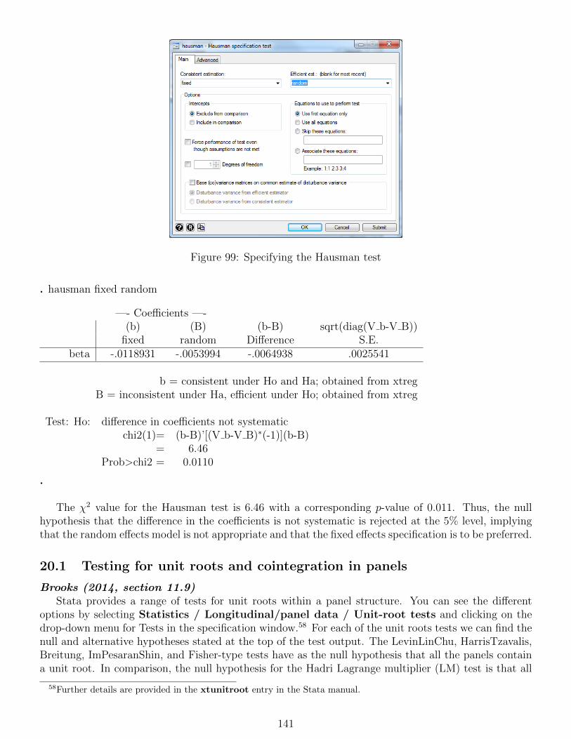
Figure 99: Specifying the Hausman test

. hausman fixed random

—- Coefficients —-(b) (B) (b-B) sqrt(diag(V b-V B))

fixed random Difference S.E.beta -.0118931 -.0053994 -.0064938 .0025541

b = consistent under Ho and Ha; obtained from xtregB = inconsistent under Ha, efficient under Ho; obtained from xtreg

Test: Ho: difference in coefficients not systematicchi2(1)= (b-B)’[(V b-V B)∗(-1)](b-B)

= 6.46Prob>chi2 = 0.0110

.

The χ2 value for the Hausman test is 6.46 with a corresponding p-value of 0.011. Thus, the nullhypothesis that the difference in the coefficients is not systematic is rejected at the 5% level, implyingthat the random effects model is not appropriate and that the fixed effects specification is to be preferred.

20.1 Testing for unit roots and cointegration in panels

Brooks (2014, section 11.9)Stata provides a range of tests for unit roots within a panel structure. You can see the different

options by selecting Statistics / Longitudinal/panel data / Unit-root tests and clicking on thedrop-down menu for Tests in the specification window.58 For each of the unit roots tests we can find thenull and alternative hypotheses stated at the top of the test output. The LevinLinChu, HarrisTzavalis,Breitung, ImPesaranShin, and Fisher-type tests have as the null hypothesis that all the panels containa unit root. In comparison, the null hypothesis for the Hadri Lagrange multiplier (LM) test is that all

58Further details are provided in the xtunitroot entry in the Stata manual.

141

the panels are (trend) stationary. Options allow you to include panel-specific means (fixed effects) andtime trends in the model of the data-generating process.

For the panel unit root test we will use the six Treasury bill/bond yields from the ‘macro.dta’workfile. Before running any panel unit root or cointegration tests, it is useful to start by examiningthe results of individual unit root tests on each series, so we run the Dickey-Fuller GLS unit root tests(dfgls) on the levels of each yield series.59 You should find that for USTB3M, USTB6M and USTB1Ythe test statistics are well below -2.5 (based on the optimal lag determined using SIC) and thus theunit root hypothesis cannot be rejected. However, for the cases of USTB3Y, USTB5Y and USTB10Ythe unit root hypothesis at the optimal lag length suggested by SIC is rejected at the 10%, 5% and 1%level, respectively.

As we know from the discussion above, unit root tests have low power in the presence of smallsamples, and so the panel unit root tests may provide different results. However, before performing apanel unit root test we have to transform the dataset into a panel format. To do so we save the currentworkfile under a new name (‘treasuryrates panel.dta’) in order to prevent the previous dataset frombeing overwritten. We will only be using the six Treasury rate series and the ‘Date’ series, so we deleteall other series. This can be easily achieved by the following command:keep Date USTB3M USTB6M USTB1Y USTB3Y USTB5Y USTB10Ywhich deletes all series but the ones specified after ‘keep’.

The next step involves reshaping the dataset into a panel format where all rate series are stackedbelow one another in one single data series. We first need to rename the series by putting a ‘rate’ infront of the series name:rename USTB3M rateUSTB3Mrename USTB6M rateUSTB6Mrename USTB1Y rateUSTB1Yrename USTB3Y rateUSTB3Yrename USTB5Y rateUSTB5Yrename USTB10Y rateUSTB10Y

Next we reshape the data from a long to a wide format. Instead of copying and pasting the individualdata sets we can use the Stata command ‘reshape’ to do this job for us. We click on Data / Createor change data / Other variable-transformation commands / Convert data between wideand long. In the window that appears (figure 100), we first select the type of transformation, i.e. Longformat from wide.

We specify the ID variable(s): Date. Then, we define the Subobservation identifier as thenew Variable: maturity (which will become the panel id) containing the different maturities of thetreasury bill series. We also check the box Allow the sub-observation identifier to include strings.Finally, we specify the Base (stub) names of X ij variables: which in our case is the rate in frontof the renamed treasury series of different maturities.60 Now the window shall resemble figure 100 andwe press OK.

We will find that the six individual treasury yield series have disappeared and there are now onlythree series in the dataset: ‘Date’, ‘maturity’ and ‘rate’. We can have a look at the data using the DataEditor. We will find that our dataset now resembles a typical panel dataset with the series of yields fordifferent maturities stacked below each other in the ‘rate’ variable, and ‘maturity’ serving as the panelid. As Stata only allows numeric variables to be a panel id we need to transform the string variable‘maturity’ into a numeric version. For this, we can use the Stata command ‘encode’. We can accessthis command by clicking on Data / Create or change data / Other variable-transformation

59A description of how to run Dickey-Fuller GLS unit root tests is explained in section 16 of this guide.60For more details and illustrative examples of how to use the ‘reshape’ command please refer to the corresponding

entry in the Stata manual.

142

Figure 100: Reshaping the Dataset into a Panel Format

commands / Encode value labels from string variable. In the specification window (figure 101),we first need to tell Stata the Source-string variable which in our case is maturity. We want tocreate a numeric version of this variable named maturity num. By clicking OK, the new variable iscreated. When checking the data type of the variable, e.g. by using the ‘codebook’ command, we shouldfind that ‘maturity num’ is a numeric variable whereas ‘maturity’ is (still) a string variable.

Figure 101: Encoding the Panel Variable

Now that all the data preparation has been done, we can finally perform the panel unit root test onthe ’rate’ series. We open the ‘xtunitroot’ specification window by selecting Statistics / Longitudi-nal/panel data / Unit-root tests. As mentioned above, there is a variety of unit root tests that wecan choose from (by clicking on the drop-down menu below Test) (figure 102, left panel). For now, wekeep the default test Levin-Lin-Chu. However, please feel free to test the sensitivities of our results toalternative test specifications. Next, we specify the Variable: rate as the variable on which we wantto perform the test.

As a final step, we click on Panel settings to specify the panel id and time id in our dataset. In

143

Figure 102: Specifying a Panel Unit Root Test

the window that appears (figure 102, right panel), we define the Panel ID variable: maturity numand the Time variable: Date and also tell Stata that our time variable is of Monthly frequency byselecting the respective option. We click OK to return to the main specification window and press OKagain to perform the test. The test output of the Levin-Lin-Chu panel unit root test is presented below.

. xtunitroot llc rate

Levin-Lin-Chu unit-root test for rateHo: Panels contain unit roots Number of panels = 6Ha: Panels are stationary Number of periods = 326

AR parameter: Common Asymptotics: N/T -> 0Panel means: IncludedTime trend: Not included

ADF regressions: 1 lagLR variance: Bartlett kernel, 22.00 lags average (chosen by LLC)

Statistic p-valueUnadjusted t -2.1370Adjusted t* 1.8178 0.9655

.

As described above, the Levin-Lin-Chu test is based on the null hypothesis that the panels containunit roots. It assumes a common p for the different panels. Looking at the test results, we find a teststatistic of 1.8178 with a corresponding p-value of 0.9655. Thus the unit root null is not rejected.

We can now re-run the panel unit root test using another test specification. What do you find? Doall tests arrive at the same solution regarding the stationarity or otherwise of the rate series? In all

144

cases, the test statistics are well below the critical values, indicating that the series contain unit roots.Thus the conclusion from the panel unit root tests are in line with the ones derived from the test of theindividual series. As some series contain a unit root and thus the panel unit root null hypothesis cannotbe rejected. Note, however, that the additional benefits from using a panel in our case might be quitesmall since the number of different panels (N = 6) is quite small, while the total number of time-seriesobservations (T = 326) is relatively large.

It is also possible to perform panel cointegration tests in Stata. However, these cointegration testsdo not come as a built-in Stata function but are in a user-written command, a so-called ado-file. Onecommand for performing panel cointegration tests has been written by Persyn & Westerlund (2008) andis based on the four panel cointegration tests developed by Westerlund (2007). It is called xtwest.61

Another panel cointegration test is available via the ado-file xtfisher and is based on the test developedby Maddala & Wu (1999).62 Finally, you can perform the panel cointegration test xtpedroni developedby Pedroni (1999, 2001).63 Independent of which command you intend to use, you can install the ado-files by typing in findit followed by the name of the command, e.g. findit xtwest. You then need tofollow the link that corresponds to the chosen command and select click here to install. We leave theimplementation of the panel cointegration test for further studies.

61For detailed references please refer to Westerlund, J. (2007) ‘Testing for error correction in panel data’. Oxford Bulletinof Economics and Statistics 69: 709-748; and Persyn, D. & Westerlund, J. (2008) ’Error-correction-based cointegrationtest for panel data’. The Stata Journal 8 (2): 232-241.

62For detailed references please refer to Maddala, G.S. & Wu, Shaowen (1999) ‘A Comparative Study of Unit RootTests With Panel Data and A New Simple Test’. Oxford Bulletin of Economics and Statistics 61: 631-652.

63For detailed references please refer to Pedroni, P. (1999) ‘Critical Values for Cointegration Tests in Heterogeneous Pan-els with Multiple Regressors’. Oxford Bulletin of Economics and Statistics 61: 653-70; and Pedroni, P. (2001) ’PurchasingPower Parity Tests in Cointegrated Panels’. Review of Economics and Statistics 83: 727-731.

145

21 Limited dependent variable models

Brooks (2014, chapter 12)Estimating limited dependent variable models in Stata is very simple. The example that will be

considered here concerns whether it is possible to determine the factors that affect the likelihood thata student will fail his/her MSc. The data comprise a sample from the actual records of failure rates forfive years of MSc students at the ICMA Centre, University of Reading, contained in the spreadsheet‘MSc fail.xls’. While the values in the spreadsheet are all genuine, only a sample of 100 students isincluded for each of the five years who completed (or not as the case may be!) their degrees in the years2003 to 2007 inclusive. Therefore, the data should not be used to infer actual failure rates on theseprogrammes. The idea for this is taken from a study by Heslop & Varotto (2007) which seeks to proposean aproach to preventing systematic biases in admissions decisions.64

The objective here is to analyse the factors that affect the probability of failure of the MSc. Thedependent variable (‘fail’) is binary and takes the value 1 if that particular candidate failed at firstattempt in terms of his/her overall grade and 0 elsewhere. Therefore, a model that is suitable forlimited dependent variables is required, such as a logit or probit.

The other information in the spreadsheet that will be used includes the age of the student, a dummyvariable taking the value 1 if the student is female, a dummy variable taking the value 1 if the studenthas work experience, a dummy variable taking the value 1 if the student’s first language is English, acountry code variable that takes values from 1 to 10.65 a dummy that takes the value 1 if the studentalready has a postgraduate degree, a dummy variable that takes the value 1 if the student achievedan A-grade at the undergraduate level (i.e. a first-class honours degree or equivalent), and a dummyvariable that takes the value 1 if the undergraduate grade was less than a B-grade (i.e. the studentreceived the equivalent of a lower second-class degree). The B-grade (or upper second-class degree)is the omitted dummy variable and this will then become the reference point against which the othergrades are compared. The reason why these variables ought to be useful predictors of the probability offailure should be fairly obvious and is therefore not discussed. To allow for differences in examinationrules and in average student quality across the five-year period, year dummies for 2004, 2005, 2006 and2007 are created and thus the year 2003 dummy will be omitted from the regression model.

First, we import the dataset into Stata. To check that all series are correctly imported we can usethe Data Editor to visually examine the imported data and the codebook command to get informationon the characteristics of the dataset. All variables should be in the numeric format and overall thereshould be 500 observations in the dataset for each series with no missing observations. Also make sureto save the workfile in the ‘.dta’-format.

To begin with, suppose that we estimate a linear probability model of Fail on a constant, Age,English, Female, Work experience, A-Grade, Below-B-Grade, PG-Grade and the year dummies. Thiswould be achieved simply by running a linear regression, using the command:regress Fail Age English Female WorkExperience Agrade BelowBGrade PGDegree Year2004Year2005 Year2006 Year2007The results would appear as below.

64Note that since this example only uses a sub-set of their sample and variables in the analysis, the results presentedbelow may differ from theirs. Since the number of fails is relatively small, I deliberately retained as many fail observationsin the sample as possible, which will bias the estimated failure rate upwards relative to the true rate.

65The exact identities of the countries involved are not revealed in order to avoid any embarrassment for students fromcountries with high relative failure rates, except that Country 8 is the UK!

146

. regress Fail Age English Female WorkExperience Agrade BelowBGrade PGDegree Year2004 Year2005Year2006 Year2007

Source SS df MS Number of obs = 500F( 11, 488) = 3.15

Model 3.84405618 11 .349459653 Prob > F = 0.0004Residual 54.1779438 488 .111020377 R-squared = 0.0663

Adj R-squared = 0.0452Total 58.022 499 .116276553 Root MSE = .3332

Fail Coef. Std. Err. t P>|t| [95% Conf. Interval]Age .0013219 .004336 0.30 0.761 -.0071976 .0098414

English -.0200731 .0315276 -0.64 0.525 -.0820197 .0418735Female -.0293804 .0350533 -0.84 0.402 -.0982545 .0394937

WorkExperience -.0620281 .0314361 -1.97 0.049 -.1237948 -.0002613Agrade -.0807004 .0377201 -2.14 0.033 -.1548142 -.0065866

BelowBGrade .0926163 .0502264 1.84 0.066 -.0060703 .1913029PGDegree .0286615 .0474101 0.60 0.546 -.0644918 .1218147Year2004 .0569098 .0477514 1.19 0.234 -.0369139 .1507335Year2005 -.0111013 .0483674 -0.23 0.819 -.1061354 .0839329Year2006 .1415806 .0480335 2.95 0.003 .0472025 .2359587Year2007 .0851503 .0497275 1.71 0.087 -.012556 .1828567

cons .1038805 .1205279 0.86 0.389 -.1329372 .3406983

.

While this model has a number of very undesirable features as discussed in chapter 12 of Brooks(2014), it would nonetheless provide a useful benchmark with which to compare the more appropriatemodels estimated below.

Next, we estimate a probit model and a logit model using the same dependent and independentvariables as above. We begin with the logit model by clicking on Statistics / Binary outcomesand choosing Logistic regression, repporting coefficients. First, we need to specify the dependentvariable (Fail) and independent variables (Age English Female WorkExperience Agrade Below-BGrade PGDegree Year2004 Year2005 Year2006 Year2007l) as shown in the upper panel offigure 103.

Next, we want to specify the standard error correction. To do so, we click on the SE/Robust taband select the Standard error type: Robust from the drop-down menu (figure 103, bottom panel).This option will ensure that the standard error estimates are robust to heteroscedasticity. Using theother tabs you can also change the optimisation method and convergence criterion. However, we do notneed to make any changes from the default, but simply click OK. The output for the logit regressionshould appear as below the figures.

147

Figure 103: Specifying a Logit Model

148

. logit Fail Age English Female WorkExperience Agrade BelowBGrade PGDegree Year2004 Year2005Year2006 Year2007, vce(robust)

Iteration 0: log pseudolikelihood = -196.96021Iteration 1: log pseudolikelihood = -181.6047Iteration 2: log pseudolikelihood = -179.72747Iteration 3: log pseudolikelihood = -179.71667Iteration 4: log pseudolikelihood = -179.71667

Logistic regression Number of obs = 500Wald chi2(11) = 31.91Prob > chi2 = 0.0008

Log pseudolikelihood = -179.71667 Pseudo R2 = 0.0875

RobustFail Coef. Std. Err. z P>|z| [95% Conf. Interval]Age .0110115 .0459359 0.24 0.811 -.0790212 .1010442

English -.1651177 .2953456 -0.56 0.576 -.7439844 .413749Female -.333894 .3601013 -0.93 0.354 -1.03968 .3718915

WorkExperience -.5687687 .2893189 -1.97 0.049 -1.135823 -.001714Agrade -1.08503 .4930358 -2.20 0.028 -2.051362 -.1186977

BelowBGrade .5623509 .3868631 1.45 0.146 -.1958868 1.320589PGDegree .2120842 .4256673 0.50 0.618 -.6222085 1.046377Year2004 .6532065 .4840248 1.35 0.177 -.2954647 1.601878Year2005 -.1838244 .5596076 -0.33 0.743 -1.280635 .9129864Year2006 1.246576 .4696649 2.65 0.008 .3260499 2.167102Year2007 .850422 .482298 1.76 0.078 -.0948648 1.795709

cons -2.256368 1.221524 -1.85 0.065 -4.650511 .1377747

.

Next we estimate the above model as a probit model. We click on Statistics / Binary outcomesbut now select the option Probit regression. We input the same model specifications as in the logitcase and again select robust standard errors. The output of the probit model is presented in the tableon the following page. As can be seen, for both models the pseudo-R2 values are quite small at justbelow 9%, although this is often the case for limited dependent variable models.

Turning to the parameter estimates on the explanatory variables, we find that only the work ex-perience and A-grade variables and two of the year dummies have parameters that are statisticallysignificant, and the Below B-grade dummy is almost significant at the 10% level in the probit specifica-tion (although less so in the logit model). However, the proportion of fails in this sample is quite small(13.4%),66 which makes it harder to fit a good model than if the proportion of passes and fails had beenmore evenly balanced. Note that Stata offers a variety of goodness-of-fit and classification tests, such asthe Hosmer-Lemeshow goodness-of-fit test. You can access these tests by selecting Statistics / Binaryoutcomes / Postestimation and then choosing the test that you would like to perform.

66Note that you can retrieve the number of observations for which ‘Fail’ takes the value 1 by using the command countif Fail==1.

149

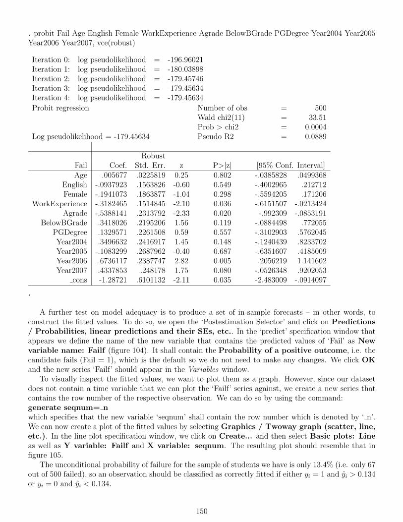
. probit Fail Age English Female WorkExperience Agrade BelowBGrade PGDegree Year2004 Year2005Year2006 Year2007, vce(robust)

Iteration 0: log pseudolikelihood = -196.96021Iteration 1: log pseudolikelihood = -180.03898Iteration 2: log pseudolikelihood = -179.45746Iteration 3: log pseudolikelihood = -179.45634Iteration 4: log pseudolikelihood = -179.45634

Probit regression Number of obs = 500Wald chi2(11) = 33.51Prob > chi2 = 0.0004

Log pseudolikelihood = -179.45634 Pseudo R2 = 0.0889

RobustFail Coef. Std. Err. z P>|z| [95% Conf. Interval]Age .005677 .0225819 0.25 0.802 -.0385828 .0499368

English -.0937923 .1563826 -0.60 0.549 -.4002965 .212712Female -.1941073 .1863877 -1.04 0.298 -.5594205 .171206

WorkExperience -.3182465 .1514845 -2.10 0.036 -.6151507 -.0213424Agrade -.5388141 .2313792 -2.33 0.020 -.992309 -.0853191

BelowBGrade .3418026 .2195206 1.56 0.119 -.0884498 .772055PGDegree .1329571 .2261508 0.59 0.557 -.3102903 .5762045Year2004 .3496632 .2416917 1.45 0.148 -.1240439 .8233702Year2005 -.1083299 .2687962 -0.40 0.687 -.6351607 .4185009Year2006 .6736117 .2387747 2.82 0.005 .2056219 1.141602Year2007 .4337853 .248178 1.75 0.080 -.0526348 .9202053

cons -1.28721 .6101132 -2.11 0.035 -2.483009 -.0914097

.

A further test on model adequacy is to produce a set of in-sample forecasts – in other words, toconstruct the fitted values. To do so, we open the ‘Postestimation Selector’ and click on Predictions/ Probabilities, linear predictions and their SEs, etc.. In the ‘predict’ specification window thatappears we define the name of the new variable that contains the predicted values of ‘Fail’ as Newvariable name: Failf (figure 104). It shall contain the Probability of a positive outcome, i.e. thecandidate fails (Fail = 1), which is the default so we do not need to make any changes. We click OKand the new series ‘Failf’ should appear in the Variables window.

To visually inspect the fitted values, we want to plot them as a graph. However, since our datasetdoes not contain a time variable that we can plot the ‘Failf’ series against, we create a new series thatcontains the row number of the respective observation. We can do so by using the command:generate seqnum= nwhich specifies that the new variable ‘seqnum’ shall contain the row number which is denoted by ‘ n’.We can now create a plot of the fitted values by selecting Graphics / Twoway graph (scatter, line,etc.). In the line plot specification window, we click on Create... and then select Basic plots: Lineas well as Y variable: Failf and X variable: seqnum. The resulting plot should resemble that infigure 105.

The unconditional probability of failure for the sample of students we have is only 13.4% (i.e. only 67out of 500 failed), so an observation should be classified as correctly fitted if either yi = 1 and yi > 0.134or yi = 0 and yi < 0.134.

150

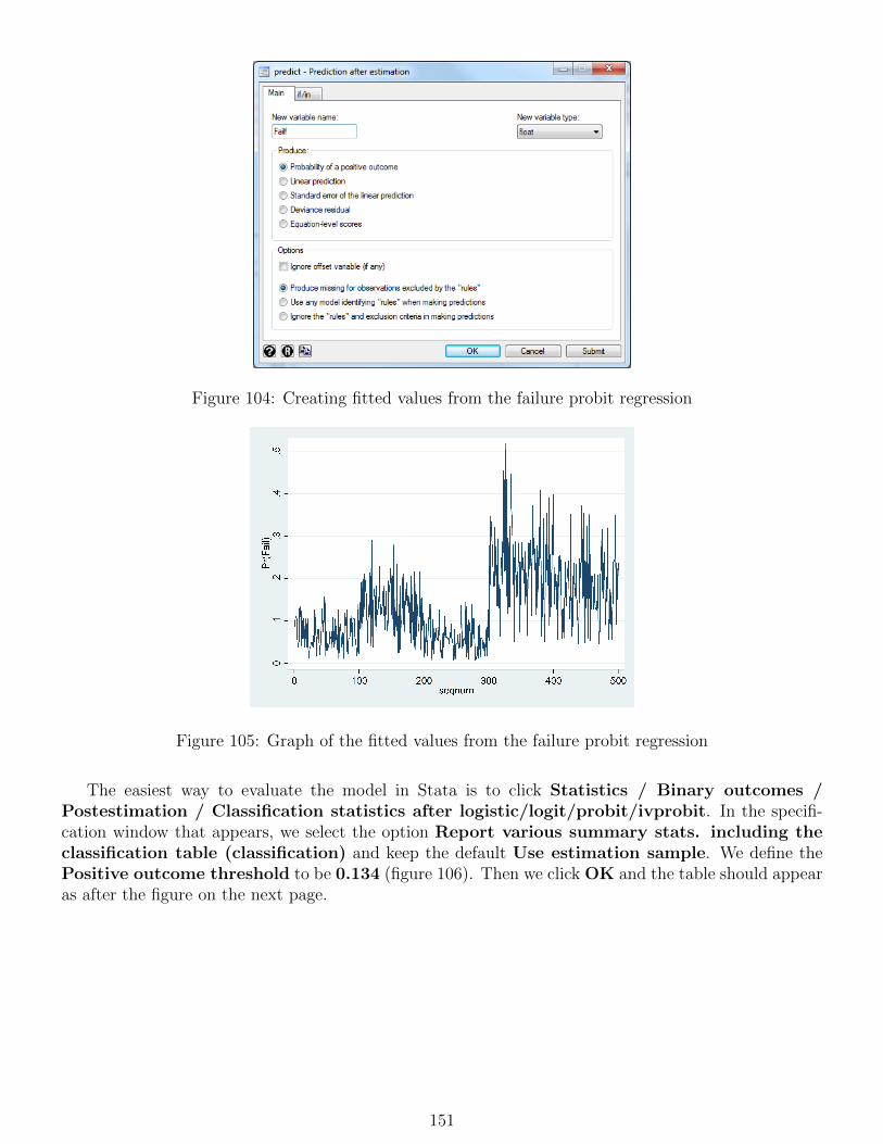
Figure 104: Creating fitted values from the failure probit regression

Figure 105: Graph of the fitted values from the failure probit regression

The easiest way to evaluate the model in Stata is to click Statistics / Binary outcomes /Postestimation / Classification statistics after logistic/logit/probit/ivprobit. In the specifi-cation window that appears, we select the option Report various summary stats. including theclassification table (classification) and keep the default Use estimation sample. We define thePositive outcome threshold to be 0.134 (figure 106). Then we click OK and the table should appearas after the figure on the next page.

151

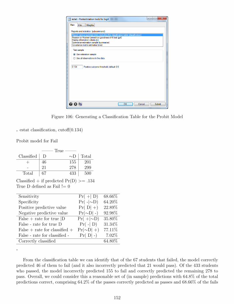
Figure 106: Generating a Classification Table for the Probit Model

. estat classification, cutoff(0.134)

Probit model for Fail

——– True ——–Classified D ∼D Total

+ 46 155 201- 21 278 299

Total 67 433 500

Classified + if predicted Pr(D) >= .134True D defined as Fail != 0

Sensitivity Pr( +| D) 68.66%Specificity Pr( -|∼D) 64.20%Positive predictive value Pr( D| +) 22.89%Negative predictive value Pr(∼D| -) 92.98%False + rate for true |D Pr( +|∼D) 35.80%False - rate for true D Pr( -| D) 31.34%False + rate for classified + Pr(∼D| +) 77.11%False - rate for classified - Pr( D| -) 7.02%Correctly classified 64.80%

.

From the classification table we can identify that of the 67 students that failed, the model correctlypredicted 46 of them to fail (and it also incorrectly predicted that 21 would pass). Of the 433 studentswho passed, the model incorrectly predicted 155 to fail and correctly predicted the remaining 278 topass. Overall, we could consider this a reasonable set of (in sample) predictions with 64.8% of the totalpredictions correct, comprising 64.2% of the passes correctly predicted as passes and 68.66% of the fails

152

correctly predicted as fails.It is important to note that we cannot interpret the parameter estimates in the usual way (see

discussion in chapter 12 in the textbook ‘Introductory Econometrics for Finance’). In order to be ableto do this, we need to calculate the marginal effects.

Figure 107: Generating Marginal Effects

Stata has an in-built command that allows to calculate marginal effects which can be accessed viaStatistics / Postestimation / Marginal analysis / Marginal means and marginal effects,fundamental analyses (figure 107, left panel). In the ‘margins’ specification window that appears(figure 107, right panel) we first need to specify the Covariate for which we want to compute marginaleffects. As we want to generate marginal effects for all of the explanatory variables we type in all inthe dialogue box. Next we select the Analysis type: Marginal effect (derivative) of covariate onoutcome. Leaving all other options to their default options and pressing OK, Stata should generatethe table of marginal effects and corresponding statistics as shown on the following page.

153

. margins, dydx( all)

Average marginal effects Number of obs = 500Model VCE RobustExpression : Pr(Fail), predict()dy/dx w.r.t. : Age English Female WorkExperience Agrade BelowBGrade PGDegree

Year2004 Year2005 Year2006 Year2007Delta-method

dy/dx Std. Err. z P>|z| [95% Conf. Interval]Age .0011179 .0044466 0.25 0.802 -.0075974 .0098331

English -.0184688 .0307689 -0.60 0.548 -.0787748 .0418372Female -.038222 .036781 -1.04 0.299 -.1103115 .0338674

WorkExperience -.0626665 .0298548 -2.10 0.036 -.1211809 -.0041521Agrade -.1060989 .0453505 -2.34 0.019 -.1949843 -.0172135

BelowBGrade .067305 .0431667 1.56 0.119 -.0173001 .1519101PGDegree .0261808 .0445415 0.59 0.557 -.0611189 .1134806Year2004 .0688528 .0477053 1.44 0.149 -.0246479 .1623536Year2005 -.0213314 .0529625 -0.40 0.687 -.125136 .0824732Year2006 .1326422 .0467502 2.84 0.005 .0410134 .2242709Year2007 .0854175 .0486634 1.76 0.079 -.009961 .180796

.

We can repeat this exercise for the logit model using the same procedure as above. Note thatwe need to re-run the logit model first and then calculate marginal effects in the same way as describedfor the probit model. If done correctly, the table of marginal effects should resemble the following:

. margins, dydx( all)

Average marginal effects Number of obs = 500Model VCE RobustExpression : Pr(Fail), predict()dy/dx w.r.t. : Age English Female WorkExperience Agrade BelowBGrade PGDegree

Year2004 Year2005 Year2006 Year2007Delta-method

dy/dx Std. Err. z P>|z| [95% Conf. Interval]Age .0011862 .0049468 0.24 0.810 -.0085095 .0108818

English -.0177866 .0318111 -0.56 0.576 -.0801353 .044562Female -.0359674 .0389302 -0.92 0.356 -.1122691 .0403343

WorkExperience -.0612683 .031165 -1.97 0.049 -.1223506 -.000186Agrade -.1168805 .0530145 -2.20 0.027 -.220787 -.012974

BelowBGrade .060577 .0416694 1.45 0.146 -.0210936 .1422476PGDegree .0228459 .045919 0.50 0.619 -.0671536 .1128454Year2004 .070364 .0523332 1.34 0.179 -.0322071 .1729352Year2005 -.0198017 .0603289 -0.33 0.743 -.1380442 .0984407Year2006 .1342824 .0505192 2.66 0.008 .0352666 .2332982Year2007 .0916083 .0517308 1.77 0.077 -.0097822 .1929987

.

154

Looking at the results, we find that not only are the marginal effects for the probit and logit modelquite similar in value, they also closely resemble the coefficient estimates obtained from the linearprobability model estimated earlier in the section.

Now that we have calculated the marginal effects, these values can be intuitively interpreted in termsof how the variables affect the probability of failure. For example, an age parameter value of around0.0012 implies that an increase in the age of the student by one year would increase the probability offailure by 0.12%, holding everything else equal, while a female student is around 3.5% less likely thana male student with otherwise identical characteristics to fail. Having an A-grade (first class) in thebachelors degree makes a candidate around 11% less likely to fail than an otherwise identical studentwith a B-grade (upper second-class degree). Finally since the year 2003 dummy has been omitted fromthe equations, this becomes the reference point. So students were more likely in 2004, 2006 and 2007,but less likely in 2005, to fail the MSc than in 2003.

155

22 Simulation Methods

22.1 Deriving critical values for a Dickey-Fuller test using simulation

Brooks (2014, section 13.7)In this and the following sub-sections we will use simulation techniques in order to model the be-

haviour of financial series. In this first example, our aim is to develop a set of critical values forDickey-Fuller test regressions. Under the null hypothesis of a unit root, the test statistic does not followa standard distribution, and therefore a simulation would be required to obtain the relevant criticalvalues. Obviously, these critical values are well documented, but it is of interest to see how one couldgenerate them. A very similar approach could then potentially be adopted for situations where therehas been less research and where the results are relatively less well known.

The simulation would be conducted in the following four steps:

1. Construct the data generating process under the null hypothesis - that is obtain a series for y thatfollows a unit root process. This would be done by:

• Drawing a series of length T , the required number of observations, from a normal distribution.This will be the error series, so that ut ∼ N(0, 1).

• Assuming a first value for y, i.e. a value for y at time t = 1.

• Constructing the series for y recursively, starting with y2, y3, and so on

y2 = y1 + u2

y3 = y2 + u3

. . .

yT = yT−1 + uT

2. Calculating the test statistic, τ .

3. Repeating steps 1 and 2 N times to obtain N replications of the experiment. A distribution ofvalues for τ will be obtained across the replications.

4. Ordering the set of N values of τ from the lowest to the highest. The relevant 5% critical valuewill be the 5th percentile of this distribution.

Some Stata code for conducting such a simulation is given below. The simulation framework considersa sample of 1,000 observations and DF regressions with no constant or trend, a constant but no trend,and a constant and a trend. 50,000 replications are used in each case, and the critical values for aone-sided test at the 1%, 5% and 10% levels are determined. The code can be found pre-written in aStata do-file entitled ‘dofile dfcv.do’.

Stata programs are simply sets of instructions saved as plain text, so that they can be written fromwithin Stata, or using a word processor or text editor. There are two types of Stata programs, do-filesand ado-files. The latter equivalent to user-written commands and once installed, can be used like anyother Stata command such as summarize or regress. The former (do-files) need to be opened everytime the user wants to run the set of commands and can be interactively adjusted. We will only dealwith do-files and leave the issue of programming ado-files for more advanced Stata users. To run ado-file, we open the Do-File Editor using the respective symbol in the Stata menu. In the window thatappears we click on File / Open... and select the ‘dofile dfcv.do’. We should now be able to see theset of Stata commands.

The different colours indicate different characteristics of the instructions. All expressions in brightblue represent Stata commands (such as ‘summarize’ or ‘regress’) and information on the individual

156

commands can be obtained typing help followed by the respective command in the Command window.Expressions in red that are expressed in double quotes mark strings and might refer to file names orpaths, value labels of variables or string values of variables. Variables in turquoise are a form of auxiliaryvariable and usually their value is substituted for a predefined content.67 Finally, text expressed in greenrepresents comments made by the Stata user. Comments are not part of the actual instructions butrather serve to explain and describe the Stata codes. There are different ways to create commentsin Stata, either by beginning the comment with ∗ or // or placing the comment between /∗ and ∗/delimiters.68 To run the program we can click on the two very right buttons in the symbol menu ofthe Do-file Editor. We have two options: (a) Execute Selection quietly (run) which will run thecode but without showing the output in the Stata Output window, and (b) Execute (do) which willprogressively report the output of the code. The latter is especially useful for debugging programs orrunning short programs, though it leads to a slower execution of the program than when running itin the quiet mode. We can also choose to run only parts of the instructions instead of the entire setof commands by highlighting the lines of commands that we would like to perform and then selectingeither of the two execution options.

The following lines of code are taken from the do-file ‘dofile dfcv.do’ which creates critical values forthe DF-test. The discussion below explains the function of the command line.

1 ∗DERIVING CRITICAL VALUES FOR A DICKEY-FULLER TEST USING MONTECARLO SIMULATIONS

2 set seed 123453 tempname tstats4 postfile ‘tstats’ t1 t2 t3 using “C:\Users\Lisa\results.dta”, replace5 quietly {6 forvalues i=1/50000 {7 drop all8 set obs 12009 generate y1=0 if n==110 replace y1=y1[ n-1]+rnormal() in 2/120011 generate dy1=y1-y1[ n-1] in 201/120012 generate lagy1=y1[ n-1]13 generate t= n-200 in 201/120014 regress dy1 lagy1, noconstant15 scalar t1= b[lagy1]/ se[lagy1]16 regress dy1 lagy117 scalar t2= b[lagy1]/ se[lagy1]18 regress dy1 t lagy119 scalar t3= b[lagy1]/ se[lagy1]20 post ‘tstats’ (t1) (t2) (t3)21 }22 }23 postclose ‘tstats’24 use “C:\Users\Lisa\results.dta”, clear25 describe26 tabstat t1 t2 t3, statistics( p1 p5 p10 ) columns(statistics)

67Macros are commonly used in Stata programming in can be applied to a variety of contexts. For more informationon the characteristics of Macros and their use in Stata, refer to the respective entry in the Stata manual.

68For more details on how to create comments in Stata please refer to the corresponding entry in the Stata manual.

157

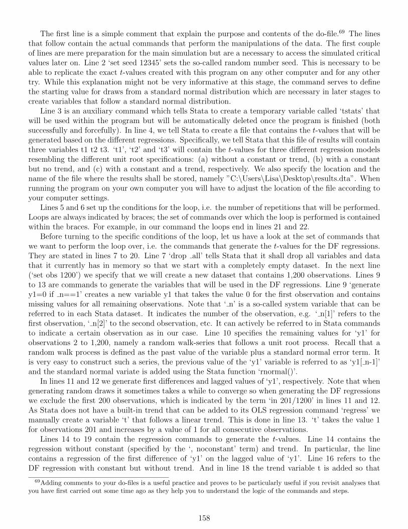
The first line is a simple comment that explain the purpose and contents of the do-file.69 The linesthat follow contain the actual commands that perform the manipulations of the data. The first coupleof lines are mere preparation for the main simulation but are a necessary to access the simulated criticalvalues later on. Line 2 ‘set seed 12345’ sets the so-called random number seed. This is necessary to beable to replicate the exact t-values created with this program on any other computer and for any othertry. While this explanation might not be very informative at this stage, the command serves to definethe starting value for draws from a standard normal distribution which are necessary in later stages tocreate variables that follow a standard normal distribution.

Line 3 is an auxiliary command which tells Stata to create a temporary variable called ‘tstats’ thatwill be used within the program but will be automatically deleted once the program is finished (bothsuccessfully and forcefully). In line 4, we tell Stata to create a file that contains the t-values that will begenerated based on the different regressions. Specifically, we tell Stata that this file of results will containthree variables t1 t2 t3. ‘t1’, ‘t2’ and ‘t3’ will contain the t-values for three different regression modelsresembling the different unit root specifications: (a) without a constant or trend, (b) with a constantbut no trend, and (c) with a constant and a trend, respectively. We also specify the location and thename of the file where the results shall be stored, namely ”C:\Users\Lisa\Desktop\results.dta”. Whenrunning the program on your own computer you will have to adjust the location of the file according toyour computer settings.

Lines 5 and 6 set up the conditions for the loop, i.e. the number of repetitions that will be performed.Loops are always indicated by braces; the set of commands over which the loop is performed is containedwithin the braces. For example, in our command the loops end in lines 21 and 22.

Before turning to the specific conditions of the loop, let us have a look at the set of commands thatwe want to perform the loop over, i.e. the commands that generate the t-values for the DF regressions.They are stated in lines 7 to 20. Line 7 ‘drop all’ tells Stata that it shall drop all variables and datathat it currently has in memory so that we start with a completely empty dataset. In the next line(‘set obs 1200’) we specify that we will create a new dataset that contains 1,200 observations. Lines 9to 13 are commands to generate the variables that will be used in the DF regressions. Line 9 ‘generatey1=0 if n==1’ creates a new variable y1 that takes the value 0 for the first observation and containsmissing values for all remaining observations. Note that ‘ n’ is a so-called system variable that can bereferred to in each Stata dataset. It indicates the number of the observation, e.g. ‘ n[1]’ refers to thefirst observation, ‘ n[2]’ to the second observation, etc. It can actively be referred to in Stata commandsto indicate a certain observation as in our case. Line 10 specifies the remaining values for ‘y1’ forobservations 2 to 1,200, namely a random walk-series that follows a unit root process. Recall that arandom walk process is defined as the past value of the variable plus a standard normal error term. Itis very easy to construct such a series, the previous value of the ‘y1’ variable is referred to as ‘y1[ n-1]’and the standard normal variate is added using the Stata function ‘rnormal()’.

In lines 11 and 12 we generate first differences and lagged values of ‘y1’, respectively. Note that whengenerating random draws it sometimes takes a while to converge so when generating the DF regressionswe exclude the first 200 observations, which is indicated by the term ‘in 201/1200’ in lines 11 and 12.As Stata does not have a built-in trend that can be added to its OLS regression command ‘regress’ wemanually create a variable ‘t’ that follows a linear trend. This is done in line 13. ‘t’ takes the value 1for observations 201 and increases by a value of 1 for all consecutive observations.

Lines 14 to 19 contain the regression commands to generate the t-values. Line 14 contains theregression without constant (specified by the ‘, noconstant’ term) and trend. In particular, the linecontains a regression of the first difference of ‘y1’ on the lagged value of ‘y1’. Line 16 refers to theDF regression with constant but without trend. And in line 18 the trend variable t is added so that

69Adding comments to your do-files is a useful practice and proves to be particularly useful if you revisit analyses thatyou have first carried out some time ago as they help you to understand the logic of the commands and steps.

158

the overall model contains both a constant and a linear trend as additional right-hand-side variables(besides ‘lagy1’). Lines 15, 17 and 19 generate the t-values corresponding to the particular models. Thecommand scalar indicates that a scalar value will be generated and the expression on the right handside of the equals sign defines the value of the scalar. It is the formula for computing the t-value, namelythe coefficient estimate on ‘lagy1’ (i.e. ‘ b[lagy1]‘) divided by the standard error of the coefficient (i.e.‘ se[lagy1]’). Line 20 tells Stata that the t-values ‘t1’, ‘t2’ and ‘t3’ for the three models shall be postedto the ‘results.dta’ file (which we have created in line 4).

If we were to execute this set of commands one time, we would generate one t-value for each of themodels. However, our aim is to get a large number of t-statistics in order to have a distribution ofvalues. Thus, we need to repeat the set of commands for the desired number of repetitions. This isdone by the loop command foreach in line 6. It states that the set of commands included in the bracesshall be executed 50,000 times (‘i=1/50000’). Note that for each of these 50,000 repetitions a new setof t-values will be generated and added to the ‘results.dta’ file so that the final version of the file shallcontain three variables (‘t1’, ‘t2’, ‘t3’) with 50,000 observations each. Finally, the ‘quietly’ in line 5 tellsStata that it shall not produce the output for the 50,000 repetitions of the DF regressions but executethe commands “quietly”. ‘postclose ‘tstats” in line 23 signals Stata that no further values will be addedto the ‘results.dta’ file.

In line 24, we tell Stata to open the file ‘results.dta’ containing the 50,000 observations of t-values.The command ‘describe’ gives us information on the characteristics of the dataset and serves merely asa check that the program has been implemented and executed successfully. Finally, line 34 provides uswith the critical values for the three different models as it generates the 1st, 5th and 10th percentile forthe three variables ‘t1’, ‘t2’, ‘t3’.

To run this program, we click on the button ‘Execute (do)’ on the very right in the toolbar of theData Editor. Note that due to the total number of 50,000 repetitions running this command will takesome time.

The critical values obtained by running the above program, which are virtually identical to thosefound in the statistical tables at the end of the textbook ‘Introductory Econometrics for Finance’,are presented in the table below (to two decimal places). This is to be expected, for the use of 50,000replications should ensure that an approximation to the asymptotic behaviour is obtained. For example,the 5% critical value for a test regression with no constant or trend and 500 observations is −1.940 inthis simulation, and −1.95 in Fuller (1976).

1% 5% 10%No constant or trend (t1) −2.56 −1.94 −1.62Constant but no trend (t2) −3.43 −2.87 −2.57Constant and trend (t3) −3.98 −3.42 −3.14

Although the Dickey–Fuller simulation was unnecessary in the sense that the critical values for theresulting test statistics are already well known and documented, a very similar procedure could beadopted for a variety of problems. For example, a similar approach could be used for constructingcritical values or for evaluating the performance of statistical tests in various situations.

22.2 Pricing Asian options

Brooks (2014, section 13.8)In this sub-section, we will apply Monte Carlo simulations to price Asian options. The steps involved

are:

1. Specify a data generating process for the underlying asset. A random walk with drift model is

159

usually assumed. Specify also the assumed size of the drift component and the assumed size ofthe volatility parameter. Specify also a strike price K, and a time to maturity, T.

2. Draw a series of length T, the required number of observations for the life of the option, from anormal distribution. This will be the error series, so that εt ∼ N(0, 1).

3. Form a series of observations of length T on the underlying asset.

4. Observe the price of the underlying asset at maturity observation T. For a call option, if the valueof the underlying asset on maturity date Pt ≤ K, the option expires worthless for this replication.If the value of the underlying asset on maturity date Pt > K, the option expires in the money, andhas a value on that date equal to PT −K, which should be discounted back to the present usingthe risk-free rate.

5. Repeat steps 1 to 4 a total of N times, and take the average value of the option over N replications.This average will be the price of the option.

A sample of Stata code for determining the value of an Asian option is given below. The example isin the context of an arithmetic Asian option on the FTSE 100, and two simulations will be undertakenwith different strike prices (one that is out of the money forward and one that is in the money forward).In each case, the life of the option is six months, with daily averaging commencing immediately, andthe option value is given for both calls and puts in terms of index options. The parameters are given asfollows, with dividend yield and risk-free rates expressed as percentages:Simulation 1 : strike=6500, risk-free=6.24, dividend yield=2.42, ‘today’s’ FTSE=6289.70, forward price=6405.35,implied volatility=26.52Simulation 2 : strike=5500, risk-free=6.24, dividend yield=2.42, ‘today’s’ FTSE=6289.70, forward price=6405.35,implied volatility=34.33

All experiments are based on 25,000 replications and their antithetic variates (total: 50,000 sets ofdraws) to reduce Monte Carlo sampling error.

Some sample code for pricing an Asian option for normally distributed errors using Stata is given asfollows:

1 ∗PRICING AN ASIAN OPTION USING MONTE CARLO SIMULATIONS2 set seed 1234563 tempname prices4 postfile ‘prices’ apval acval using “C:\Users\Lisa\asianoption.dta”, replace5 quietly {6 forvalues i=1/25000 {7 drop all8 set obs 1259 local obs=12510 local ttm=0.511 local iv=0.2812 local rf=0.062413 local dy=0.024214 local dt=‘ttm’/ N15 local drift=(‘rf’-‘dy’-(‘iv’ˆ(2)/2.0))∗‘dt’16 local vsqrdt=‘iv’∗(‘dt’ˆ(0.5))17 local k=550018 local s0=6289.719 generate rands=rnormal()

160

20 generate spot=‘s0’∗exp(‘drift’+‘vsqrdt’∗rands) in 121 replace spot=spot[ n-1]∗exp(‘drift’+‘vsqrdt’∗rands) in 2/‘obs’22 summarize spot, meanonly23 scalar av=r(mean)24 if av>‘k’ {25 scalar acval=(av-‘k’)∗exp(-‘rf’∗‘ttm’)26 }27 else {28 scalar acval=029 }30 if av<‘k’ {31 scalar apval=(‘k’-av)∗exp(-‘rf’∗‘ttm’)32 }33 else {34 scalar apval=035 }36 post ‘prices’ (apval) (acval)37 scalar drop av acval apval38 replace rands=-rands39 replace spot=‘s0’∗exp(‘drift’+‘vsqrdt’∗rands) in 140 replace spot=spot[ n-1]∗exp(‘drift’+‘vsqrdt’∗rands) in 2/‘obs’41 summarize spot, meanonly42 scalar av=r(mean)43 if av>‘k’ {44 scalar acval=(av-‘k’)∗exp(-‘rf’∗‘ttm’)45 }46 else {47 scalar acval=048 }49 if av<‘k’ {50 scalar apval=(‘k’-av)∗exp(-‘rf’∗‘ttm’)51 }52 else {53 scalar apval=054 }55 post ‘prices’ (apval) (acval)56 }57 }58 postclose ‘prices’59 use “C:\Users\Lisa\asianoption.dta”, clear60 describe61 quietly {62 summarize acval63 scalar callprice=r(mean)64 summarize apval65 scalar putprice=r(mean)66 }67 display callprice

161

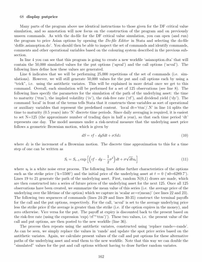
68 display putprice

Many parts of the program above use identical instructions to those given for the DF critical valuesimulation, and so annotation will now focus on the construction of the program and on previouslyunseen commands. As with the do-file for the DF critical value simulation, you can open (and run)the program to price Asian options by opening the Do-file Editor in Stata and selecting the do-file‘dofile asianoption.do’. You should then be able to inspect the set of commands and identify commands,comments and other operational variables based on the colouring system described in the previous sub-section.

In line 4 you can see that this program is going to create a new workfile ‘asianoption.dta’ that willcontain the 50,000 simulated values for the put options (‘apval’) and the call options (‘acval’). Thefollowing lines define how these values are generated.

Line 6 indicates that we will be performing 25,000 repetitions of the set of commands (i.e. sim-ulations). However, we will still generate 50,000 values for the put and call options each by using a“trick”, i.e. using the antithetic variates. This will be explained in more detail once we get to thiscommand. Overall, each simulation will be performed for a set of 125 observations (see line 8). Thefollowing lines specify the parameters for the simulation of the path of the underlying asset: the timeto maturity (‘ttm’), the implied volatility (‘iv’), the risk-free rate (‘rf’), and dividend yield (‘dy’). Thecommand ‘local’ in front of the terms tells Stata that it constructs these variables as sort of operationalor auxiliary variables that represent the predefined content. ‘local dt=‘ttm’/ N’ in line 14 splits thetime to maturity (0.5 years) into ‘N’ discrete time periods. Since daily averaging is required, it is easiestto set N=125 (the approximate number of trading days in half a year), so that each time period ‘dt’represents one day. The model assumes under a risk-neutral measure that the underlying asset pricefollows a geometric Brownian motion, which is given by

dS = rf - dySdt + σSdz (10)

where dz is the increment of a Brownian motion. The discrete time approximation to this for a timestep of one can be written as

St = St−1 exp[(

rf - dy− 1

2σ2)

dt + σ√dtut

](11)

where ut is a white noise error process. The following lines define further characteristics of the optionssuch as the strike price (‘k=5500’) and the initial price of the underlying asset at t = 0 (‘s0=6289.7’).Lines 19 to 21 generate the path of the underlying asset. First, random N(0,1) draws are made, whichare then constructed into a series of future prices of the underlying asset for the next 125. Once all 125observations have been created, we summarize the mean value of this series (i.e. the average price of theunderlying over the lifetime of the option) which we capture in ‘scalar av=r(mean)’ (see lines 22 and 23).The following two sequences of commands (lines 24-29 and lines 30-35) construct the terminal payoffsfor the call and the put options, respectively. For the call, ‘acval’ is set to the average underlying priceless the strike price if the average is greater than the strike (i.e. if the option expires in the money), andzero otherwise. Vice versa for the put. The payoff at expiry is discounted back to the present based onthe risk-free rate (using the expression ‘exp(-‘rf’∗‘ttm’)’). These two values, i.e. the present value of thecall and put options, are then posted to the new workfile (line 36).

The process then repeats using the antithetic variates, constructed using ‘replace rands=-rands’.As can be seen, we simply replace the values in ‘rands’ and update the spot price series based on theantithetic variates. Again, we calculate present values of the call and put options for these alternativepaths of the underlying asset and send them to the new workfile. Note that this way we can double the”simulated” values for the put and call options without having to draw further random variates.

162

Strike = 6500, IV = 26.52 Strike = 5500, IV = 34.33CALL Price CALL PriceAnalytical Approximation 203.45 Analytical Approximation 888.55Monte Carlo Normal 206.43 Monte Carlo Normal 887.96

PUT Price PUT PriceAnalytical Approximation 348.7 Analytical Approximation 64.52Monte Carlo Normal 350.79 Monte Carlo Normal 62.76

This completes one cycle of the loop, which will then be repeated for further 24,999 times and overallcreate 50,000 values for the call and put options each. Once the loop has finished, we can open thenew workfile ‘asianoption.dta’ which contains the 50,000 simulated values using the command in line59. It is useful to ‘describe’ the contents in the dataset first to check that the program has successfullycreated the option values. We can also look at the results using the Data Editor, and we will see thatthe dataset contains two arrays ‘acval’ and ‘apval’, which comprise 50,000 rows of the present value ofthe call and put option for each simulated path. The last thing that we then need to do is calculate theoption prices as the averages over the 50,000 replications. This is done in lines 61 to 66. Once this setof commands has been executed the call price and the option price are displayed in the Output window.For the specifics stated above, the call price is approximately 857.23 and the put price lies around 32.26.

Note that both call values and put values can be calculated easily from a given simulation, since themost computationally expensive step is in deriving the path of simulated prices for the underlying asset.In the following table, we compare the simulated call and put prices for different implied volatilities andstrike prices along with the values derived from an analytical approximation to the option price, derivedby Levy, and estimated using VBA code in Haug (1998, pp. 97–100).

The main difference between the way that the simulation is conducted here and the method used forStata simulation of the Dickey–Fuller critical values is that here, the random numbers are generated byopening a new series called ‘rands’ and filling it with the random number draws. The reason that thismust be done is so that the negatives of the elements of rands can later be taken to form the antitheticvariates. Finally, for each replication, the ‘if’ clause will set out of the money call prices (where k>av)and out of the money put prices (k<av) to zero. Then the call and put prices for each replication arediscounted back to the present using the risk-free rate, and outside of the replications loop, the optionsprices are the averages of these discounted prices across the 50,000 replications.

In both cases, the simulated option prices are quite close to the analytical approximations, althoughthe Monte Carlo seems to overvalue the out-of-the-money call and to undervalue the out-of-the-moneyput. Some of the errors in the simulated prices relative to the analytical approximation may result fromthe use of a discrete-time averaging process using only 125 data points.

22.3 VaR estimation using bootstrapping

Brooks (2014, section 13.9)The following Stata code can be used to calculate the MCRR for a ten-day holding period (the

length that regulators require banks to employ) using daily S& P500 data, which is found in the file‘sp500.dta’. The code is presented followed by an annotated copy of some of the key lines.

1 ∗CALCULATION OF MCRR FOR A 10-DAY HORIZON USING BOOTSTRAP-PING

2 \\Bootstrap Loop3 preserve4 set seed 123455 gen n= n

163

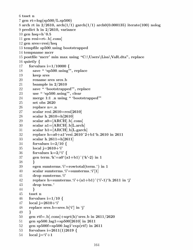
6 tsset n7 gen rt=log(sp500/L.sp500)8 arch rt in 2/2610, arch(1/1) garch(1/1) arch0(0.000135) iterate(100) nolog9 predict h in 2/2610, variance10 gen hsq=hˆ0.511 gen resi=rt- b[ cons]12 gen sres=resi/hsq13 tempfile sp500 using bootstrapped14 tempname mcrr15 postfile ‘mcrr’ min max using “C:\Users\Lisa\VaR.dta”, replace16 quietly {17 forvalues i=1/10000 {18 save “ ‘sp500 using’”, replace19 keep sres20 rename sres sres b21 bsample in 2/261022 save “ ‘bootstrapped’”, replace23 use “ ‘sp500 using’”, clear24 merge 1:1 n using “ ‘bootstrapped’”25 set obs 262026 replace n= n27 scalar resi 2610=resi[2610]28 scalar h 2610=h[2610]29 scalar a0=[ARCH] b[ cons]30 scalar a1=[ARCH] b[L.arch]31 scalar b1=[ARCH] b[L.garch]32 replace h=a0+a1∗resi 2610ˆ2+b1∗h 2610 in 261133 scalar h 2611=h[2611]34 forvalues i=2/10 {35 local j=2610+‘i’36 forvalues k=2/‘i’ {37 gen term ‘k’=a0∗(a1+b1)ˆ(‘k’-2) in 138 }39 egen sumterms ‘i’=rowtotal(term ∗) in 140 scalar sumterms ‘i’=sumterms ‘i’[1]41 drop sumterms ‘i’42 replace h=sumterms ‘i’+(a1+b1)ˆ(‘i’-1)∗h 2611 in ‘j’43 drop term ∗

44 }45 tsset n46 forvalues i=1/10 {47 local j=2610+‘i’48 replace sres b=sres b[‘i’] in ‘j’49 }50 gen rtf= b[ cons]+sqrt(h)∗sres b in 2611/262051 gen sp500 lag1=sp500[2610] in 261152 gen sp500f=sp500 lag1∗exp(rtf) in 261153 forvalues i=2611(1)2619 {54 local j=‘i’+1

164

55 replace sp500 lag1=sp500f[‘i’] in ‘j’56 replace sp500f=sp500 lag1∗exp(rtf) in ‘j’57 }58 summarize sp500f59 scalar min=r(min)60 scalar max=r(max)61 post ‘mcrr’ (min) (max)62 drop in 2611/262063 drop sres b sp500f sp500 lag1 rtf merge64 }65 }66 postclose ‘mcrr’67 use “C:\Users\Lisa\VaR.dta”, clear68 //Long and Short positions69 gen l1=log(min/1138.73)70 quietly {71 summarize l172 scalar mcrrl=1-exp((-1.645∗r(sd))+r(mean))73 gen s1=log(max/1138.73)74 summarize s175 scalar mcrrs=exp((1.645∗r(sd))+r(mean))-176 }77 //Calculation of minimum risk requirements78 display mcrrl79 display mcrrsAgain, annotation of the Stata code will concentrate on commands that have not been discussed

previously. The first lines of command set up the dataset for the further analyses. As we will bechanging the dataset throughout the program we start our program with the command ‘preserve’ whichsaves the dataset in its current stage and guarantees that it will be restored to this stage once the programhas ended. Note that when starting your program with the command ‘preserve’ it even restores thedataset to its initial state when the program is not executed entirely, e.g. due to a bug in the program ordue to pressing ‘break’. We also create a new variable ‘ n’ as a substitute for the missing time variablein the dataset and ‘tsset’ the data to this variable. This is necessary as some of the commands that wewill use later only work when ‘tsset’ is performed.

The command ‘gen rt=log(sp500/L.sp500)’ in line 7 creates continuously compounded returns whichare the dependent variable in the GARCH(1,1) model, i.e. one ARCH and one GARCH term, thatis estimated in the following line. As we lose one data point when calculating returns we only per-form the estimation for observations 2 to 2610. We set a starting value for the ARCH term with‘arch0(0.000135)’70 and allow the process to perform up to 100 iterations (‘iterate(100)’). The meanequation of the model contains a constant only, which is automatically included by Stata, so we onlyneed to specify the dependent variable ‘rt’ in the regression command. The following line generates aseries of the fitted conditional variances for the model which are stored in the series ‘h’. The three lines‘gen hsq=hˆ0.5’, ‘gen resi=rt- b’ and ‘gen sres=resi/hsq’ will construct a set of standardised residuals.

Next we set up a set of (temporary) files that we will use within the bootstrap loop to temporarilystore subsets of the data as well as to store our final estimates from the repetition. In particular,

70We chose this starting value to make the estimates comparable to those generated using EViews. However, the startingvalues can also be set to a different value. Detailed explanations of Stata’s default choices regarding starting values canbe found in the manual entry for the command ‘arch’.

165

the command ‘tempfile sp500 using bootstrapped’ in line 13 creates two auxiliary files that will beautomatically deleted after the program has ended and serve to temporarily store a subset of the data.The ‘postfile’ command should be well-known from the previous simulation examples and sets up thefile ‘VaR.dta’ to store the results of the bootstrap loop.

Next follows the core of the program, which involves the bootstrap loop. The number of replicationshas been defined as 10,000. What we want to achieve is to re-sample the series of standardised residuals(‘sres’) by drawing randomly with replacement from the existing dataset. However, as only the ‘sres’series shall be re-sampled while all the other data series shall remain in their current order, we needto transfer the ‘sres’ data series to the temporary file ‘bootstrapped’, perform the re-sampling and re-import the re-sampled series into the full data set. This is achieved by the set of commands in lines 18to 24. Note that the command ‘bsample’ is the command performing the actual bootstrapping whilethe other results are merely auxiliary commands to store and merge the bootstrapped dataset. In orderto distinguish the bootstrapped standardised residuals from the original series we rename the series to‘sres b’ before merging it with the full dataset.

The next block of commands constructs the future path of the S&P500 return and price series overthe ten-day holding period. The first step to achieve this is to extend the sample period to include 10further observations, i.e. observations 2611 to 2620, and also to update the variable ‘n’ to these furtherdata points. Unfortunately, Stata does not allow us to simply extend some of the series to these newobservations so we need to manually tell Stata which values to input in the new cells. We start withextending the conditional variance series by adding forecasts of this series for the observations 2611 to2620. This is achieved by the commands in lines 26 to 43. Recall from chapter 9.17 in the textbook‘Introductory Econometrics for Finance’ that the one-step-ahead forecast of the conditional variance is

hf1,T = α0 + α1u2T + βhT ,

where hT is the conditional variance at time T, i.e. the end of the in-sample period, and uT is thesquared disturbance term at time T, and α0, α1 and β are the coefficient estimates obtained from theGARCH(1,1) model estimated over the observations 2 to 2610;and the s-step-ahead forecast can be produced by

hfs,T = α0

s−1∑i=1

(α1 + β)i−1 + (α1 + β)s−1hf1,T ,

for any values of s ≥ 2.First we create a set of scalars that contain the end-of-sample squared disturbance term (‘resi 2610’)

and the end-of-sample conditional variance (‘h 2610’) as well as three scalars containing the estimatedcoefficients (‘a0’, ‘a1’ and ‘b1’). Then, we generate the one-step-ahead forecast of h according to theformula above and place the value in observation 2611 of the series ‘h’. We also save this value as a scalaras we will be using it to create the further multiple-step-ahead forecasts. The two- to ten-step-aheadforecasts are generated in lines 33 to 43 and their values are placed in the observations 2612 to 2620,respectively. While this line of code uses two loops that translate the above equation for s-step aheadforecasts into Stata commands, we could alternatively have written down the individual equations foreach of the two- to ten-step-ahead forecasts.71

71The code to do so would look something like this:replace h=a0+(a1+b1)∗h 2611 in 2612replace h=a0+a0∗(a1+b1)+((a1+b1)ˆ2)∗h 2611 in 2613replace h=a0+a0∗(a1+b1)+a0∗(a1+b1)ˆ2+((a1+b1)ˆ3)∗h 2611 in 2614replace h=a0+a0∗(a1+b1)+a0∗(a1+b1)ˆ2+a0∗(a1+b1)ˆ3+((a1+b1)ˆ4)∗h 2611 in 2615replace h=a0+a0∗(a1+b1)+a0∗(a1+b1)ˆ2+a0∗(a1+b1)ˆ3+a0∗(a1+b1)ˆ4+((a1+b1)ˆ5)∗h 2611 in 2616replace h=a0+a0∗(a1+b1)+a0∗(a1+b1)ˆ2+a0∗(a1+b1)ˆ3+a0∗(a1+b1)ˆ4+a0∗(a1+b1)ˆ5+((a1+b1)ˆ6)∗h 2611 in 2617replace h=a0+a0∗(a1+b1)+a0∗(a1+b1)ˆ2+a0∗(a1+b1)ˆ3+a0∗(a1+b1)ˆ4+a0∗(a1+b1)ˆ5+a0∗(a1+b1)ˆ6+((a1+b1)ˆ7)∗h 2611

in 2618replace h=a0+a0∗(a1+b1)+a0∗(a1+b1)ˆ2+a0∗(a1+b1)ˆ3+a0∗(a1+b1)ˆ4+a0∗(a1+b1)ˆ5+a0∗(a1+b1)ˆ6+a0∗(a1+b1)ˆ7+

((a1+b1)ˆ8)∗h 2611 in 2619

166

Once the conditional variance forecasts are created, we take the first ten observations of the re-sampled standardised residuals and place them in observations 2611 to 2620 of series ‘sres b’. This isachieved by the set of commands in lines 46 to 48. Now, we are able to generate values for the S&P500return series over the added 10-day holding period. The command‘gen rtf= b[ cons]+sqrt(h)∗sres b in 2611/2620’creates a new variable of “forecasted” returns which are calculated as the coefficient on the constantfrom the mean equation of the GARCH(1,1) model (‘ b[ cons]’) plus the product of the square rootof the conditional variance (‘squrt(h)’) and the bootstrapped standardised residuals (‘sres b’). Usingthese “forecasted” return series we can now construct the path of the S&P500 price series based on theformula:

sp500ft = sp500t−1e

rtft

This formula is translated into Stata code in lines 50 to 56. In these lines we first create a series oflagged S&P500 prices and then generate the “forecasts” of the series over ten days.

Finally, we obtain the minimum and maximum values of the S&P500 series over the ten days andstore them in the variables ‘min’ and ‘max’ in the data file ‘VaR.dta’.

This set of commands is then repeated 10,000 times so that after the final repetition there will be10,000 minimum and maximum values for the S&P500 prices in ‘VaR.dta’.

The final block of commands generates the MCRR for a long and a short position in the S&P500. Thefirst step is to construct the log returns for the maximum loss over the ten-day holding period, which forthe long position is achieved by the command ‘gen l1=log(min/1138.73)’ and for the short position by‘gen s1=log(max/1138.73)’. We now want to find the 5th percentile of the empirical distribution of themaximum losses for the long and short positions. Under the assumption that the ‘l1’ and ‘s1’ statisticsare normally distributed across the replications, the MCRR can be calculated by the commandsscalar mcrrl=1-exp((-1.645∗r(sd))+r(mean)) andscalar mcrrs=exp((1.645∗r(sd))+r(mean))-1 , respectively.

The results generated by running the above program should be displayed in the Stata Output windowand should approximate to:

MCRR=0.04436604 for the long position, andMCRR=05284345 for the short position.

These figures represent the minimum capital risk requirement for a long and short position, respectively,as a percentage of the initial value of the position for 95% coverage over a 10-day horizon. This meansthat, for example, approximately 4.4% of the value of a long position held as liquid capital will besufficient to cover losses on 95% of days if the position is held for 10 days. The required capital to cover95% of losses over a 10-day holding period for a short position in the S&P500 index would be around5.3%. This is as one would expect since the index had a positive drift over the sample period. Therefore,the index returns are not symmetric about zero as positive returns are slightly more likely than negativereturns. Higher capital requirements are thus necessary for a short position since a loss is more likelythan for a long position of the same magnitude.

replace h=a0+a0∗(a1+b1)+a0∗(a1+b1)ˆ2+a0∗(a1+b1)ˆ3+a0∗(a1+b1)ˆ4+a0∗(a1+b1)ˆ5+a0∗(a1+b1)ˆ6+a0∗(a1+b1)ˆ7+a0∗(a1+b1)ˆ8+((a1+b1)ˆ9)∗h 2611 in 2620

167

23 The Fama-MacBeth procedure

Brooks (2014, section 14.10)In this section we will perform the two-stage Fama-MacBeth procedure. The Fama-MacBeth pro-

cedure as well as related asset pricing tests are described in the sub-sections in 14.10 in the textbook‘Introductory Econometrics for Finance’. There is nothing particularly complex about the two-stageprocedure – it only involves two sets of standard linear regressions. The hard part is really in collectingand organising the data. If we wished to do a more sophisticated study – for example, using a boot-strapping procedure or using the Shanken correction, this would require more analysis then is conductedin the illustration below. However, hopefully the Stata code and the explanations will be sufficient todemonstrate how to apply the procedures to any set of data.

The example employed here is taken from the study by Gregory, Tharyan and Chistidis (2013) thatexamines the performance of several different variants of the Fama-French and Carhart models using theFama-MacBeth methodology in the UK following several earlier studies showing that these approachesappear to work far less well for the UK than the US. The data required are provided by Gregory et al.on their web site.72 Note that their data have been refined and further cleaned since their paper waswritten (i.e. the web site data are not identical to those used in the paper) and as a result the parameterestimates presented here deviate slightly from theirs. However, given that the motivation for this exerciseis to demonstrate how the Fama-MacBeth approach can be used in Stata, this difference should not beconsequential. The two data files used are ‘monthlyfactors.csv’ and ‘vw sizebm 25groups.csv’. Theformer file includes the time series of returns on all of the factors (smb, hml, umd, rmrf, the return onthe market portfolio (rm) and the return on the risk-free asset (rf)), while the latter includes the timeseries of returns on twenty-five value-weighted portfolios formed from a large universe of stocks, two-waysorted according to their sizes and book-to-market ratios.

The first step in this analysis for conducting the Fama-French or Carhart procedures using themethodology developed by Fama and MacBeth is to create a new Stata workfile which we call ‘ff example.dta’and to import the two csv data files into it. The data in both cases run from October 1980 to December2012, making a total of 387 data points. However, in order to obtain results as close as possible tothose of the original paper, when running the regressions, the period is from October 1980 to December2010 (363 data points). We then need to set up a do-file along the lines of those set up in the previoussub-sections to conduct the two-stage procedure. It is called ‘dofile famafrench’.

1 ∗THE FAMA-MACBETH PROCEDURE IN STATA2 /∗ Save a snapshot of the file in its current state ∗/3 snapshot save4 /∗ Transform actual returns into excess returns ∗/5 quietly {6 foreach var of varlist SL S2 S3 S4 SH S2L S22 S23 S24 S2H M3L M32 M33 M34

M3H B4L B42 B43 B44 B4H BL B2 B3 B4 BH {7 replace ‘var’=‘var’-rf8 }9 }10 /∗ Define number of time series observations ∗/11 local obs=36312 /∗ Run the first stage time-series regressions separately for each portfolio and13 store the betas in a separate workfile ∗/14 tempname betas

72http://business-school.exeter.ac.uk/research/areas/centres/xfi/research/famafrench/files.

168

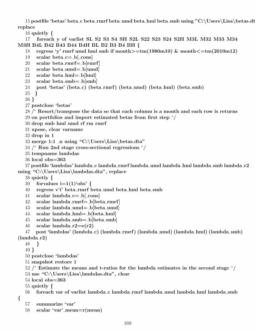
15 postfile ‘betas’ beta c beta rmrf beta umd beta hml beta smb using ”C:\Users\Lisa\betas.dta”,replace

16 quietly {17 foreach y of varlist SL S2 S3 S4 SH S2L S22 S23 S24 S2H M3L M32 M33 M34

M3H B4L B42 B43 B44 B4H BL B2 B3 B4 BH {18 regress ‘y’ rmrf umd hml smb if month>=tm(1980m10) & month<=tm(2010m12)19 scalar beta c= b[ cons]20 scalar beta rmrf= b[rmrf]21 scalar beta umd= b[umd]22 scalar beta hml= b[hml]23 scalar beta smb= b[smb]24 post ‘betas’ (beta c) (beta rmrf) (beta umd) (beta hml) (beta smb)25 }26 }27 postclose ‘betas’28 /∗ Resort/transpose the data so that each column is a month and each row is returns29 on portfolios and import estimated betas from first step ∗/30 drop smb hml umd rf rm rmrf31 xpose, clear varname32 drop in 133 merge 1:1 n using “C:\Users\Lisa\betas.dta”34 /∗ Run 2nd stage cross-sectional regressions ∗/35 tempname lambdas36 local obs=36337 postfile ‘lambdas’ lambda c lambda rmrf lambda umd lambda hml lambda smb lambda r2

using “C:\Users\Lisa\lambdas.dta”, replace38 quietly {39 forvalues i=1(1)‘obs’ {40 regress v‘i’ beta rmrf beta umd beta hml beta smb41 scalar lambda c= b[ cons]42 scalar lambda rmrf= b[beta rmrf]43 scalar lambda umd= b[beta umd]44 scalar lambda hml= b[beta hml]45 scalar lambda smb= b[beta smb]46 scalar lambda r2=e(r2)47 post ‘lambdas’ (lambda c) (lambda rmrf) (lambda umd) (lambda hml) (lambda smb)

(lambda r2)48 }49 }50 postclose ‘lambdas’51 snapshot restore 152 /∗ Estimate the means and t-ratios for the lambda estimates in the second stage ∗/53 use “C:\Users\Lisa\lambdas.dta”, clear54 local obs=36355 quietly {56 foreach var of varlist lambda c lambda rmrf lambda umd lambda hml lambda smb

{57 summarize ‘var’58 scalar ‘var’ mean=r(mean)

169

59 scalar ‘var’ tratio=sqrt(‘obs’)∗r(mean)/r(sd)60 }61 summarize lambda r262 scalar lambda r2 mean=r(mean)63 }64 display lambda c mean65 display lambda c tratio66 display lambda rmrf mean67 display lambda rmrf tratio68 display lambda umd mean69 display lambda umd tratio70 display lambda hml mean71 display lambda hml tratio72 display lambda smb mean73 display lambda smb tratio74 display lambda r2 mean

Before starting with the actual two-stage Fama-MacBeth procedure we save a snapshot of the currentstate of the workfile (‘snapshot save’, line 3). This is useful as we will be performing transformationsof the data in the file that are irreversible (once performed). If a snapshot of the file is saved thanwe can always return to the file at the state at which the snapshot was saved, undoing all the datamanipulations that were undertaken in the meantime.

We can think of the remainder of this program as comprising of several sections. The first step is totransform all of the raw portfolio returns into excess returns which are required to compute the betas inthe first stage of Fama-MacBeth (lines 6 and 7). This is fairly simple to do and we just write over theoriginal series with their excess return counterparts. The command ’local obs=363’ in line 11 ensuresthat the same sample period as the paper by Gregory et al. is employed throughout.

Next we run the first stage of the Fama-MacBeth procedure, i.e. we run a set of time-series regressionsto estimate the betas. We want to run the Carhart 4-factor model separately for each of the twenty-fiveportfolios. A Carhart 4-factor model regresses a portfolio return on the excess market return (‘rmrf’),the size factor (‘smb’), the value factor (‘hml’) and the momentum factor (‘umd’). Since the independentvariables remain the same across the set of regressions and we only change the dependent variable, i.e.the excess return of one of the twenty-five portfolios, we can set this first stage up as a loop. Lines 13to 27 specify this loop. In particular, the lines of command specify that for each of the 25 variableslisted behind the term ‘varlist’, Stata shall perform an OLS regression of the portfolio’s excess return(indicated by the ‘y’ which is to be replaced by the particular portfolio return listed in the loop) on the4 factors. Note that we restrict the sample for this model to the period October 1980 to December 2012(if month>=tm(1980m10) & month<=tm(2010m12)) instead of using the whole sample.

We need to store the estimates from these regressions into separate series for each parameter. Thisis achieved by the commands in lines 14 and 15 as well as lines 24 and 27. In particular, the command‘postfile’ sets up a new file named ‘betas.dta’ in which the beta coefficients on the four factors plus theconstant are saved. Thus, for each of the twenty-five portfolios we will generate four beta estimatesthat will then be posted to the file ‘betas.dta’. After the loop has ended, the file ‘betas.dta’ will contain25 observations for the six variables ‘beta c’, ‘beta rmrf’, ‘beta umd’, ‘beta hml’ and ‘beta smb’. Toillustrate this further, the loop starts off with the excess return on portfolio ‘SL’ (the first item in the‘varlist’) and the coefficient estimates from the 4-factor model (‘beta c’ ‘beta rmrf’ ‘beta umd’ ‘beta hml’‘beta smb’) will be transferred to the ‘betas.dta’ file as the first entry for each variable. Then Statamoves on to the second variable in the ‘varlist’, i.e. the excess return on portfolio ‘S2’, and will perform

170

the 4-factor model and save the coefficient estimates in ‘betas.dta’. They will constitute the second entryin the beta series. Stata will continue with this procedure until it has performed the set of commandsfor the last variable in the list, i.e. ‘BH’. The beta coefficients for the regressions using ‘BH’ as thedependent variable will be the 25th entry in the file ‘betas.dta’.

So now we have run the first step of the Fama-MacBeth methodology – we have estimated thebetas, also known as the factor exposures. The slope parameter estimates for the regression of a givenportfolio (i.e. ‘beta rmrf’, ‘beta umd’, ‘beta hml’, ‘beta smb’) will show how sensitive the returns onthat portfolio are to the corresponding factors and the intercepts (‘betas c’) will be the Jensen’s alphaestimates. These intercept estimates stored in ‘beta c’ should be comparable to those in the secondpanel of Table 6 in Gregory et al. – their column headed ‘Simple 4F ’. Since the parameter estimatesin all of their tables are expressed as percentages, we need to multiply all of the figures given from theStata output by 100 to make them on the same scale. If the 4-factor model is a good one, we shouldfind that all of these alphas are statistically insignificant. We could test this individually if we wishedby adding an additional line of code in the loop to save the t-ratio in the regressions (such as ‘scalarbeta c tratio= b[ cons]/ se[ cons]’).

The second stage of the Fama-MacBeth procedure is to run a separate cross-sectional regressionfor each point in time. An easy way to do this is to, effectively, rearrange/transpose the data so thateach column represents one month and the rows are the excess returns of one of the 25 portfolio. InStata this can be easily achieved by the command ‘xpose, clear’ (line 31). ‘xpose’ transposes the data,changing variables into observations and observations into variables. The supplement ‘varname’ addsthe variable ‘ varname’ to the transposed data containing the original variable names. The command‘xpose’ deletes untransposed data so that after the execution the dataset cannot be returned to itsprevious stage. To prevent our original data getting lost, we have saved the state of the data prior toany transformations. For the second stage analysis, we will not be using the time-series factors andvariables ‘smb’, ‘hml’, ‘umd’, ‘rf’, ‘rm’ and ‘rmrf’ so we drop these from the dataset prior to transposingthe data (line 30). Then we transpose the data in line 31. Note that Stata has allocated new variablenames to the observations, which are constructed as ‘v’ plus the position of the observation in theprevious dataset. For example, all data points in the first row (of the previous dataset) correspondingto October 1980 are now stored in ‘v1’; all data points in the second row corresponding to November1980 are now stored in ‘v2’; and so on. The first row of the transposed dataset contains the months(though in numeric coding). We drop this observation to make each row correspond to one of the 25portfolios (line 32). Thus, the first column contains the excess returns of all 25 portfolios for October1980 and the last column contains the excess returns of the 25 portfolios for December 2012.

Finally, we merge the transformed dataset with the betas estimated at the first stage of Fama-MacBeth (line 33), which basically involves adding these variables to the existing dataset. This isnecessary as these variables will serve as the independent variables in the second stage of Fama-MacBeth.

We are now in a position to run the second-stage cross-sectional regressions corresponding to thefollowing equation:73

Ri = α + λMβi,M + λSβi,S + λV βi,V + λUβi,U + eiThis is performed in lines 41 to 56. Again, it is more efficient to run this set of regressions in aloop. In particular, we regress each of the variables (i.e. ‘v1’, ‘v2’, ‘v3’,..,‘v387’) representing theexcess returns of the 25 portfolios for a particular month on the beta estimates from the first stage(i.e. ‘beta rmrf’, ‘beta umd’, ‘beta hml’ and ‘beta smb’). Then we store the coefficients on these factorexposures in the scalars ‘lambda c’, ‘lambda rmrf’, ‘lambda umd’, ‘lambda hml’, and ‘lambda smb’.‘lambda c’ will contain all intercepts from the second stage regressions, ‘lambda rmrf’ will contain allparameter estimates on the market risk premium betas, and so on. We also collect the R2 values foreach regression in the scalar ‘lambda r2’ as it is of interest to examine the cross-sectional average. We

73See chapter 14.10.2 for a derivation of this equation.

171

store these lambdas in the file ‘lambdas.dta’.Note that the command ‘forvalues i=1(1)‘obs” in line 39 indicates that we restrict the sample to

December 2010 to make it comparable to Gregory et al.. Thus, the first regression will be of ‘v1’ corre-sponding to October 1980 on a constant, beta rmrf, beta umd, beta hml and beta smb with the estimatesbeing stored in the first row of the variables ‘lambda c’, ‘lambda rmrf’, ‘lambda umd’, ‘lambda hml’,‘lambda smb’ and ‘lambda r2’ in the file ‘lambdas.dta’. The second regression will be of ‘v2’ corre-sponding to November 1980 on the set of betas and the estimates will be stored in the second row in‘lambdas.dta’. This will go on until ‘v363’ corresponding to December 2010 and the lambda estimatesfor this regression will be reported in row 363 of ‘lambdas.dta’. Finally, we restore the dataset to itsinitial state with the command ‘snapshot restore’ (line 51). The estimates saved in the files ‘betas.dta’and ‘lambdas.dta’ will not become lost when executing this command.

The final stage of the Fama-MacBeth procedure is to estimate the averages and standard deviationsof these estimates using something equivalent to the following equations, respectively for each parameter.The average value over t of λj,t can be calculated as

λj = 1TFMB

TFMB∑t=1

λj,t , j = 1, 2, 3, 4, ...

To do this we first ‘summarize’ each of the variables – however, without actually producing theoutput (note that we use the ‘quietly’ command) and then create a scalar containing the mean ofthe variable (‘scalar ‘var’ mean=r(mean)’) and a scalar containing the t-ratio of the estimate (‘scalar‘var’ tratio=sqrt(‘obs’)∗r(mean)/r(sd)’). Thus ‘lambda c mean’ will contain the mean of the cross-sectional intercept estimates, and the corresponding t-ratio will be stored in ‘lambda c tratio’ and soon. Note that we loop this step in order to preserve space. Finally we tell Stata to display these values(lines 64 to 74) in order to inspect the results of the Fama-MacBeth procedure. The lambda parameterestimates should be comparable with the results in the columns headed ‘Simple 4F Single’ from PanelA of Table 9 in Gregory et al. Note that they use γ to denote the parameters which have been called λin this text. The parameter estimates obtained from this simulation and their corresponding t-ratio aregiven in the table below. Note that the latter do not use the Shanken correction as Gregory et al. do.These parameter estimates are the prices of risk for each of the factors, and interestingly only the priceof risk for value is significantly different from zero.

Parameter Estimate t-ratioCons 0.34 0.89λ M 0.21 0.46λ S 0.08 0.50λ V 0.42 2.23λ U 0.32 0.50

172