University of California, Santa Cruz Department of Economics ECON 294A (Fall 2014) - Stata Lab Instructor: Manuel Barron 1 Econometric Tools 1: Non-Parametric Methods 1 Introduction This lecture introduces some of the most basic tools for non-parametric estimation in Stata. Non-parametric econometrics is a huge field, and although the essential ideas are pretty intuitive, the concepts get complicated fairly quickly. This lecture is meant to give you some background knowledge of non-parametric methods in econometrics. If you are interested in using non-parametric methods more in depth, there are many textbooks at different levels of sophistication. For instance “Non-parametric Econometrics” by Pagan and Ullah is fairly accessible, but if you would like more advanced treatment (one year PhD level course) you may want to use Li and Racine’s “Non-parametric Econometrics: Theory and Practice” textbook, which is the standard non-parametric econometrics textbook in graduate programs. In parametric methods we need to make assumptions about the distribution of the distur- bance term (for instance, normality) or about the shape of the relation between the variables under analysis (for instance, linearity). The main advantage of non-parametric methods is that they require making none of these assumptions. The most basic non-parametric methods provide appealing ways to analyze data, like plotting histograms or densities. These methods also allow to plot bivariate relationships (relations between two variables). Since the results of non-parametric estimation are typically presented as graphs, it becomes essential to produce nicely formatted graphs, so in this lecture we’ll get a bit deeper into graph options, choosing line width, colors, pattern, etc. Non-parametric methods are very useful to study relations between two variables, but including more and more variables in the analysis results in the errors. This is commonly known as the curse of dimensionality. Since we will use graphic methods, we will ignore this problem by now. 1 Please contact me with any comments (typos, errors, unclear stuff, or other suggestions on how to improve these notes) at mbarron4 [at] ucsc 1

Welcome message from author
This document is posted to help you gain knowledge. Please leave a comment to let me know what you think about it! Share it to your friends and learn new things together.
Transcript
University of California, Santa CruzDepartment of EconomicsECON 294A (Fall 2014) - Stata LabInstructor: Manuel Barron1
Econometric Tools 1:Non-Parametric Methods
1 Introduction
This lecture introduces some of the most basic tools for non-parametric estimation in Stata.Non-parametric econometrics is a huge field, and although the essential ideas are prettyintuitive, the concepts get complicated fairly quickly. This lecture is meant to give you somebackground knowledge of non-parametric methods in econometrics. If you are interestedin using non-parametric methods more in depth, there are many textbooks at differentlevels of sophistication. For instance “Non-parametric Econometrics” by Pagan and Ullahis fairly accessible, but if you would like more advanced treatment (one year PhD levelcourse) you may want to use Li and Racine’s “Non-parametric Econometrics: Theory andPractice” textbook, which is the standard non-parametric econometrics textbook in graduateprograms.
In parametric methods we need to make assumptions about the distribution of the distur-bance term (for instance, normality) or about the shape of the relation between the variablesunder analysis (for instance, linearity). The main advantage of non-parametric methods isthat they require making none of these assumptions.
The most basic non-parametric methods provide appealing ways to analyze data, likeplotting histograms or densities. These methods also allow to plot bivariate relationships(relations between two variables). Since the results of non-parametric estimation are typicallypresented as graphs, it becomes essential to produce nicely formatted graphs, so in thislecture we’ll get a bit deeper into graph options, choosing line width, colors, pattern, etc.
Non-parametric methods are very useful to study relations between two variables, butincluding more and more variables in the analysis results in the errors. This is commonlyknown as the curse of dimensionality. Since we will use graphic methods, we will ignore thisproblem by now.
1Please contact me with any comments (typos, errors, unclear stuff, or other suggestions on how toimprove these notes) at mbarron4 [at] ucsc
1

2 Density Estimation
2.1 Histogram
A histogram is a graphical representation of the distribution of a continuous random variable.To construct a histogram, we first split the data in intervals called bins, covering the entirerange of the variable at hand. For instance, if the variable takes values from 0.5 to 3.5,the bins could be [0.5,1.0], ]1.0,1.5], ]1.5,2.0], ]2.0,2.5], ]2.5,3.0], ]3.0,3.5]. Then, count thenumber of times the variable falls in each bin. Finally, draw a rectangle with base determinedby the bin and height determined by the number of times the data falls in that bin.
If we plot the histogram of “hours per day” in Stata, we will get
Figure 1 - Histogram
0.2
.4.6
.8D
ensi
ty
0 1 2 3 4hours per day
Note that the shape will depend on bin width: if we split the data in more bins than the“optimal” we’ll get:
Figure 2 - Histogram with too many bins
0.2
.4.6
.8D
ensi
ty
0 1 2 3 4hours per day
2

If, on the other hand, we split the data in “too few” bins, we get a graph like the onebelow. The choice of bins is a little more advanced than we want to go, so for any practicalpurpose I would stick to Stata’s default number of bins (unless you have a compelling reasonto choose a particular bin width).
Figure 3 - Histogram with too few bins
0.2
.4.6
Den
sity
0 1 2 3hours per day
do-file
clear all
set seed -7
set obs 200
cd [set your working directory]
gen x = 5*uniform()+5
gen y = 2 + sin(x) + 0.25*rnormal()
la var y "hours per day"
la var x "wage"
hist y, graphregion(color(white))
graph export "hist1.pdf", replace
hist y, bin(30) graphregion(color(white))
graph export "hist2.pdf", replace
hist y, bin(5) graphregion(color(white))
graph export "hist3.pdf", replace
hist y, graphregion(color(white))
graph export "kernel_1.pdf", replace
3
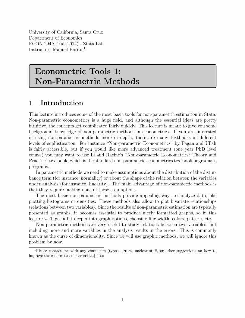
2.2 Kernel Density Estimation
Kernel Density Estimation is a method to estimate the probability density function of a ran-dom variable. Based on the observed sample, kernel density estimation allows to make infer-ence about the variable distribution in the population. It can be thought of as a “smooth”version of the histogram.
Figure 4 - Kernel Density Estimate0
.2.4
.6D
ensi
ty
0 1 2 3 4hours per day
kernel = epanechnikov, bandwidth = 0.2063
Kernel density estimate
Figure 5 - Kernel Density and Histogram
0.2
.4.6
.8
0 1 2 3 4
Density kdensity y
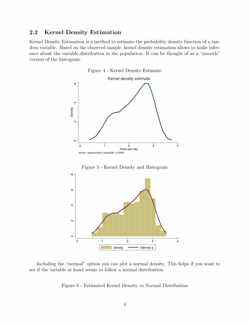
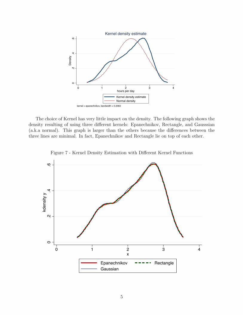
Including the “normal” option you can plot a normal density. This helps if you want tosee if the variable at hand seems to follow a normal distribution.
Figure 6 - Estimated Kernel Density vs Normal Distribution
4
0.2
.4.6
Den
sity
0 1 2 3 4hours per day
Kernel density estimateNormal density
kernel = epanechnikov, bandwidth = 0.2063
Kernel density estimate
The choice of Kernel has very little impact on the density. The following graph shows thedensity resulting of using three different kernels: Epanechnikov, Rectangle, and Gausssian(a.k.a normal). This graph is larger than the others because the differences between thethree lines are minimal. In fact, Epanechnikov and Rectangle lie on top of each other.
Figure 7 - Kernel Density Estimation with Different Kernel Functions
0.2
.4.6
kden
sity
y
0 1 2 3 4x
Epanechnikov Rectangle Gaussian
5

On the other hand, bandwidth is central to the shape of the density. There are manymethods of optimal bandwidth choice, but this is an advanced topic. My recommendationis to simply use Stata’s default optimal bandwidth (if you are interested, it is chosen bycross-validation).
Stata lets you choose a bandwidth different than the default. If you pick a narrow band-width (less than the optimal) you will produce an “undersmoothed” kernel. It is called undersmoothed because it has many “jumps”. Some of these jumps are present in this dataset,but not in the true population, so we should ignore them. Knowing what to ignore is tricky,by now just rely on Stata’s optimal bandwidth.If, on the other hand, you choose to wide a bandwidth, the resulting graph is “oversmoothed”,which means it misses some of the most important features of the density
Figure 8 - Kernel Density Estimation with Different Bandwidths
0.2
.4.6
.8kd
ensi
ty y
0 1 2 3 4hourly wage
bandwidth = 0.21 bandwidth = 0.80bandwidth = 0.10
.
6
do-file
twoway (hist y, graphregion(color(white))) ///
|| (kdensity y, graphregion(color(white)) lwidth(thick))
graph export "kernel_hist.pdf", replace
twoway (kdensity y, epan legend(label(1 Epanechnikov)) lcolor(red) lw(thick)) ///
|| (kdensity y, rectangle legend(label(2 Rectangle)) lpattern(dash) lw(thick) ///
lcolor(dkgreen)) ///
|| (kdensity y, gaussian legend(label(3 Gaussian)) lcolor(dknavy)) ///
, graphregion(color(white))
graph export "kernel_comparison.pdf", replace
twoway ///
|| (kdensity y, lwidth(thick) legend(label(1 "bandwidth = 0.21"))) ///
|| (kdensity y, bw(.80) legend(label(2 "bandwidth = 0.80"))) ///
|| (kdensity y, bw(.10) legend(label(3 "bandwidth = 0.10"))) ///
, graphregion(color(white)) xtitle(hourly wage)
kdensity y, normal graphregion(color(white)) lwidth(thick)
graph export "kernel4.pdf", replace
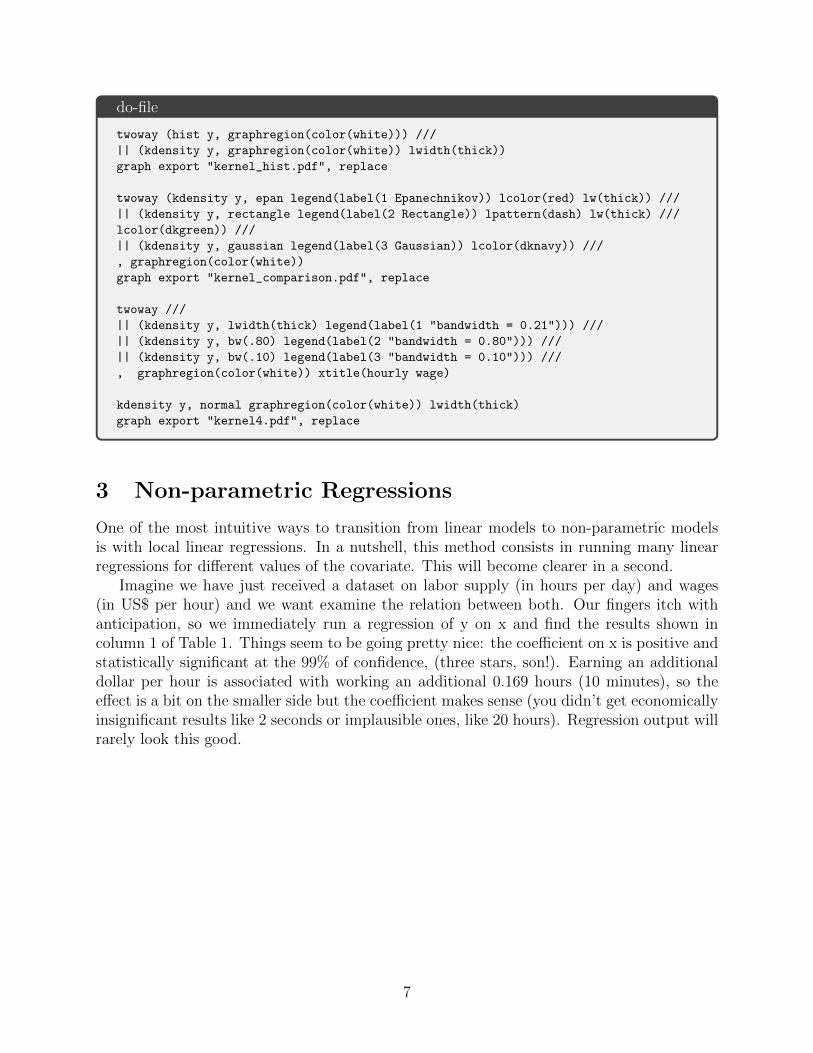
3 Non-parametric Regressions
One of the most intuitive ways to transition from linear models to non-parametric modelsis with local linear regressions. In a nutshell, this method consists in running many linearregressions for different values of the covariate. This will become clearer in a second.
Imagine we have just received a dataset on labor supply (in hours per day) and wages(in US$ per hour) and we want examine the relation between both. Our fingers itch withanticipation, so we immediately run a regression of y on x and find the results shown incolumn 1 of Table 1. Things seem to be going pretty nice: the coefficient on x is positive andstatistically significant at the 99% of confidence, (three stars, son!). Earning an additionaldollar per hour is associated with working an additional 0.169 hours (10 minutes), so theeffect is a bit on the smaller side but the coefficient makes sense (you didn’t get economicallyinsignificant results like 2 seconds or implausible ones, like 20 hours). Regression output willrarely look this good.
7

Table 1: Wages and Labor Supply, OLS
(1) (2)hours per day hours per day
wage 0.169*** 0.806***(0.031) (0.028)
high wage 12.489***(0.493)
wage x high wage -1.588***(0.058)
Constant 0.950*** -3.127***(0.237) (0.187)
Observations 200 200
Notes: wage: hourly wage in US$; high wage takes the value of 1 if hourly wage is greater than 8 US$ andzero otherwise. Standard errors in parenthesis. * p<0.10, **, p<0.05, *** p<0.01.
Figure 9 - Wage and Labor Supply, linear fit
01
23
4
5 6 7 8 9 10wage
However, Figure 9 shows that things aren’t going so well with OLS. OLS provides thebest linear fit, but the best linear fit is misleading in this case. There is a clear inverse-Urelationship between x and y. Eyeballing it, the slope is positive for hourly wages between$5 and 8, and negative for hourly wages between $8 and 10. You can think of income effectscoming at play for hourly wages above $8.
Given that we believe the relation to be positive from 5-8 and negative 8-10, we couldinclude an interaction term in the regression to allow for a change in slope.
8

Figure 10 - Piecewise Linear OLS
01
23
4
5 6 7 8 9 10wage
Figure 10 - Piecewise Linear OLS, with “smaller bandwidth”
01
23
4
5 6 7 8 9 10wage
9

twoway (scatter y x, mcolor(gray) msize(small)) ///
|| (lfit y x, lcolor(black) lwidth(thick)) ///
, legend(off) graphregion(color(white))
twoway (scatter y x, mcolor(gray) msize(small)) ///
|| (lfit y x if x<8, lcolor(black) lwidth(thick)) ///
|| (lfit y x if x>=8, lcolor(black) lwidth(thick)) ///
, legend(off) graphregion(color(white))
twoway (scatter y x, mcolor(gray) msize(small)) ///
|| (lfit y x if x>=5 & x<6, lcolor(black) lwidth(thick)) ///
|| (lfit y x if x>=6 & x<7, lcolor(black) lwidth(thick)) ///
|| (lfit y x if x>=7 & x<8, lcolor(black) lwidth(thick)) ///
|| (lfit y x if x>=8 & x<9, lcolor(black) lwidth(thick)) ///
|| (lfit y x if x>=9 & x<10, lcolor(black) lwidth(thick)) ///
, legend(off) graphregion(color(white))
The above procedures may work if we are absolutely sure of where are the breakingpoints. But if we are not, we may want to use a non-parametric estimator, like local linearregressions. Local linear regression runs linear regressions locally meaning, in a neighborhoodof x, i.e. within a given bandwidth. For instance, to estimate the slop at x=6, local linearregression takes all the data with x between 5.5 and 6.5, and estimates the slope at thatpoint. Then, it moves to 6.1, takes all the points between 5.6 and 6.6 to estimate a newslope. Since both sets contain basically the same points, the slopes are going to be verysimilar, so the function looks continuous. Local polynomials (lpoly) goes a step further andincludes polynomials in x to improve the estimation. Figure 11 shows the results
Figure 11 - Local polynomial estimators
01
23
4
5 6 7 8 9 10
do-file
twoway (scatter y x, mcolor(gray) msize(small)) ///
|| (lpoly y x, lcolor(black) lwidth(thick)) ///
, legend(off) graphregion(color(white))
10

Figure 12 - OLS, piecewise linear regression, Local Polynomials
11.5
22.5
3
5 6 7 8 9 10
do-file
twoway (lpoly y x, lcolor(gray) lwidth(thick) lpattern(dash)) ///
|| (lfit y x if x>=5 & x<6, lcolor(black) lwidth(thick)) ///
|| (lfit y x if x>=6 & x<7, lcolor(black) lwidth(thick)) ///
|| (lfit y x if x>=7 & x<8, lcolor(black) lwidth(thick)) ///
|| (lfit y x if x>=8 & x<9, lcolor(black) lwidth(thick)) ///
|| (lfit y x if x>=9 & x<10, lcolor(black) lwidth(thick)) ///
|| (lfit y x, lcolor(red)) ///
, legend(off) graphregion(color(white))
4 Alternative Non-Parametric Regression Commands
Together with poly, fpfit, lowess provide easy ways of estimating bivariate relations non-parametrically.
The options are pretty similar to those in poly. I will not cover them in lecture, but youmay be asked to use them in the assignment or in the final exam.
The main difference between the methods seems to be at the extreme values of wages.This is because at wages close to 5 or 10, there are not many data points to the left (or theright), so the use of different weighting functions will likely produce slightly different results.
As with the choice of kernel, there is little difference in the method you use. The mostimportant thing is the bandwidth used in the estimation. Choice of bandwidth is an advancedtopic, so by now you should just use the default bandwidth chosen by Stata.
11

Figure 13 - Alternative Non-parametric Methods
11.5
22.5
3
5 6 7 8 9 10
lpoly lowessfracpoly
do-file
twoway (lpoly y x, legend(label(1 "lpoly"))) ///
|| (lowess y x, legend(label(2 "lowess"))) ///
|| (fpfit y x, legend(label(3 "fracpoly"))) ///
, graphregion(color(white))
12

5 Confidence Bands
In a regression table, the point estimate doesn’t tell the whole story. For instance, weneed standard errors to build confidence intervals, which allow us to infer if a coefficient issignificant or not. Similarly, in non-parametric analysis we can produce confidence bands.
An easy way of generating confidence bands is with the “ci” versions of lpoly and fpfit.For instance: lpolyci.
do-file
twoway (lpolyci y x), graphregion(color(white))
Figure 14 - Local Polynomials with Confidence Bands
11.
52
2.5
3
5 6 7 8 9 10lpoly smoothing grid
95% CI lpoly smooth: hours per day
The above command allows us to create quick plots with confidence intervals. However,if we want to change some options we may run into a bit of trouble. For instance, if wechange the line color to black, the resulting graph may not be what we were hoping for.
do-file
twoway (lpolyci y x, lcolor(black)), graphregion(color(white))
13
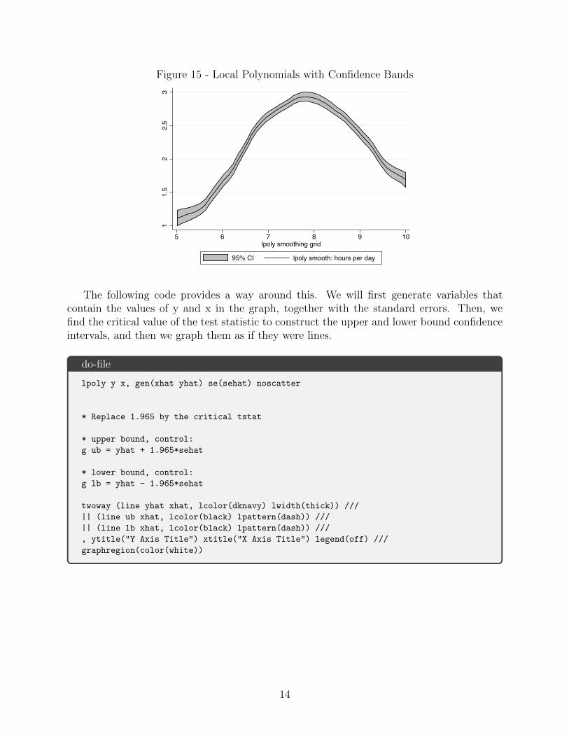
Figure 15 - Local Polynomials with Confidence Bands
11.
52
2.5
3
5 6 7 8 9 10lpoly smoothing grid
95% CI lpoly smooth: hours per day
The following code provides a way around this. We will first generate variables thatcontain the values of y and x in the graph, together with the standard errors. Then, wefind the critical value of the test statistic to construct the upper and lower bound confidenceintervals, and then we graph them as if they were lines.
do-file
lpoly y x, gen(xhat yhat) se(sehat) noscatter
* Replace 1.965 by the critical tstat
* upper bound, control:
g ub = yhat + 1.965*sehat
* lower bound, control:
g lb = yhat - 1.965*sehat
twoway (line yhat xhat, lcolor(dknavy) lwidth(thick)) ///
|| (line ub xhat, lcolor(black) lpattern(dash)) ///
|| (line lb xhat, lcolor(black) lpattern(dash)) ///
, ytitle("Y Axis Title") xtitle("X Axis Title") legend(off) ///
graphregion(color(white))
14

Figure 16 - Local Polynomials with Confidence Bands
11.
52
2.5
3Y
Axis
Titl
e
5 6 7 8 9 10X Axis Title
15
Related Documents