ECE 661 - Homework-10 · ECE 661 - Homework-10 Vishveswaran Jothi [email protected] 11-26-2016 1 Theory and Implementation Image Reconstruction 1.1 Introduction The given task to

ECE 661 - Homework-10

Vishveswaran [email protected]

11-26-2016

1 Theory and Implementation Image Reconstruction

1.1 IntroductionThe given task to find 3D coordinates of a given pair of stereo images by finding the funda-

mental matrix that relates the images. Then reconstruct the 3D image from the Camera matricesand Fundamental matrix by triangulating the position of the world coordinate that corresponds tothe pixels in the image coordinates of the ordered image pair. Note that the reconstructed imagewould have projective distortion, since we cannot find unique P, P’ from the fundamental matrix.

The Implementation is separated into three sections namely

1. Finding Fundamental Matrix and 3D Reconstruction with projective distortion

2. Image rectification

3. Detecting Interest points Using SURF and canny Edge detectors

Theory of SURF is not explained, since we have covered it extensively in class.

1.2 Finding Fundamental MatrixThe algorithm to find fundamental matrix and to refine it using Non linear least squares method(Levenberg Marquandt) is explained in the section in algorithmic manner. Appropriate mathemati-cal equations are also used for better understanding.

Pre-requisites before proceeding with the algorithm is to manually get the 8 corresponding co-ordinates from the both images, since we do not implement combination RANSAC and interestpoint detectors which will the program robust and autonomous, but in turn will make the imple-mentation complicated.

Step1: Get the 8 corresponding point from the images.

Step2: Since the raw points do not yield good results as per hartley and Zisserman algorithm,we find a normalized value for pixel coordinates such that mean is zero and the distance is

√2 from

the center, which is at (0,0). Let the homographies be T1,T2.

1

Step3: Use the 8 normalized corresponding points to get approximate Fundamental matrix us-ing the below equation.

Af = 0

where A is given by

A =[xi′xi xi′yi xi′ yi′xi yi′yi xi yi 1

]where f= [F11 F12 F13 F21 F22 F23 F31 F32 F33]

Step4:Using SVD solve for Fundamental matrix (F), the last right eigenvector is the F matrix.

Step5: Condition the F matrix thus obtained using the constraint that F has the rank of 2. Thatis find SVD of F and set the last Diagonal element to zero. Then reconstruct F by mutliplying allthe components of SVD.

UDV T = svd(F )

Set D(last) =0. Finally reconstruct F=UDVT .

Step6: Once obtained get the final F matrix estimation by the below formula.

F = T2TfT1

Step7: Since this Yield poor results we will find optimized F such that it gives low geometric errorusing LM optimization. Both with and without LM for F matrix is shown below.

Step8: First we need P, P’ to construct Xworld that is 3D point in world coordinate.where P,P’ is given by

P = [I3X3|0]

andP ′ = [[e′]xF |e′]

The e and e’ are the right and left null vectors of F.

Step9: Finally we get Xworld by using AXworld=0 and set

||Xworld|| = 1

where A is given by

A =

xiP

3T − P 1T

yiP3T − P 2T

x′iP

′3T − P ′1T

y′iP′3T − P ′2T

since,

P =

P 1T

P 2T

P 3T

2

lllrly,

P ′ =

P ′1T

P ′2T

P ′3T

Step10: Now generate the error function that will be used to optimize the F. The error function isprojecting the world coordinate using P and P’ to the respective image coordinates and finding thesquare of euclidean distance with the already existing coordinates.

d2geom = Σ(||xi − xpi||2 + ||x′i − xp′i||2)

where xp=PXworld and xp’=P’Xworld

Step11: Use the above error function to get the optimized F matrix using LM non linear squareoptimization.

Step12: For reconstructing the 3D point using the images use step 7 with the corresponding pointsobtained from the SURF interest point detector.while P’ is obtained from the optimized F

1.3 Image RectificationIn this section, we discuss about the algorithm used for image rectification which will make theepipolar of the images go to infinity thus making the search for the correspondence point in thesecond image pair on the same row. But due to the error in the data points, we need to look for thebest match in the few rows around the same row in the image pair one.Step1: We first rotate the second image by T1 matrix. Then find the angle of epipole with respectto x axis then rotate the entire image so that epipole goes to x axis.

e′ =

f01

Step2: Now use the G matrix to send the epipole along the x axis to infinity along x axis. so Gmatrix is given by

G =

1 0 00 1 0−1/f 0 1

After multiplying this with the image we get the epipole at

e =

f00

Step3: Apply the transformation matrix T2 to get it back with the center.

Step4: The overall homography matrix is given by H=T2GRT1.

3

Step5: The homography for the first image is found using a linear least squares minimizationprocedure to minimize the sum of squares distances given by

minH1Σd(H1xi, Hx′i)

This places a additional constraint of having epipolar lines at same rows.

Step5: The extensive detailing of the procedure is found at Multiple View Geometry by RichardHartley and Andrew Zisserman. Here it is briefly explained so that students can proceed for imple-mentation.H,H’ is a matching pair only if [He]xH=[H’e’]xH’M

He = (1 + aTH ′e′)H ′e′

The above is the sufficient condition to set matching pair of H, H’. Since we know that H’ will takee’ to (1,0,0)T . The final equation is H=I+(1,0,0)T aT . Therefore, H is given by

H =

a b c0 1 00 0 1

So we have to minimize

Σ(axi + byi + c− x′i)2

. We use linear method to solve this and to get the output of H, which will send the epipoles toimage 1 to infinity.

1.4 Detecting Interest points Using SURF and canny Edge detectorsIn this section,we discuss about how canny edge detector can be used to find the interest points

in the image. Since we know how to extract interest points using SURF that we know the theoryand implementation from homework 4.

Step1: Load the images from the file path obtained from the user along with parameters requiredfrom the canny edge detector.

Step2: Use the in built canny edge detector from Matlab/ opencv in python.

Step3: Now use the edge points obtained in the canny edge detector as the interest points andconsider a window around it to be used as a descriptor for the interest point. Use NCC to obtain thebest match in the second image in the ordered pair.

Step4: Also use an additional constraint that the corresponding pixel coordinate in the secondimage should be in ± few rows from the row of the pixel in the first image.

Step5: Since we have already rectified the images the above condition will be satisfied while theobtaining the best match.

Step6: The image rectification sends both the epipolar point to infinity. Making the images fallin parallel plane.

4

Step7: The correspondence thus found is used to send the image back into the 3D world pointand hence the we can reconstruct the 3D image using the step 7 of previous procedure.

1.5 Performance of SURF based and Canny based 3D ReconstructionThe major challenge that I faced was with the images, if the images are not proper then it will

not give us proper results a sample for that is shown in the output section where the points weredetected on few edges of the not all. Hence the output was not clear. We cannot understand the 3Dreconstructed image.

1. The effect of the non linear optimization of F matrix is not significant for the initial esti-mate which is the without any rectification of the images. Since we manually choose thecorresponding points it yield better results.

2. But if we don’t do the non linear optimization for the next part with surf points the initialestimate F will not yield better results, It fails when we try to make it rank 2. Hence the nonlinear optimization using LM is required especially, when we have corresponding points notacquired manually.

3. The other difference is found when we use the canny edge detector and the surf points tofind the F matrix. Depending on the number of matches the F matrix varies and the 3Dreconstruction is different for both since they don’t have same no.of correct correspondence.

4. Canny edge for the current image gives poor results.

Figure 1: Image which has matching point with wrong value

5

Figure 2: 3D Reconstruction of Image which has matching point with wrong value

The F matrix on manually correspondence is

F =

3.59565935560240e− 08 9.96294460548003e− 08 −0.000456045271900163−3.20849191472748e− 07 1.04069761275889e− 07 0.00304754380408788

0.000281497739757546 −0.00299536205208598 0.314415893630868

The F matrix on manually correspondence after optimization is

F =

−3.59026038771700e− 08 −9.96465357027825e− 08 0.0004560452719240373.20478611822560e− 07 −1.03952460979274e− 07 −0.00304754380410895−0.000281497739827248 0.00299536205204712 −0.314415893630868

The epipole on image 1 with manually correspondence before rectification is

e =

0.99460.10410.0001

The epipole on image 2 with manually correspondence before rectification is

ep =

−0.9896−0.1442−0.0000

6

The P of image2 with manually correspondence before rectification is

P ′ =

−4.05829134e− 05 0.00043183466 −0.04532852250 −0.9895532590.00027855700 −0.00296407028 0.311131289 −0.144167769

3.22306653e− 07 −8.85006777e− 08 −0.00308145393 −3.79226773e− 05

The F matrix on Rectified image is

F =

−4.94454402159479e− 25 5.23822005708923e− 19 −9.68482810874193e− 20−5.87847157169025e− 20 −1.34226591767741e− 07 −0.003249484444892992.59081908065319e− 17 0.00320759632191316 −0.141792735762057

The F matrix on Rectified image after optimization is

F =

−4.63968738722312e− 33 −5.23822005708932e− 19 9.68482810874451e− 205.87847157169025e− 20 1.34226591767741e− 07 0.00324948444489299−2.59081908065319e− 17 −0.00320759632191316 0.141792735762057

The epipole on rectified image 1 is

e =

18.86065098607525e− 151.77244672842534e− 17

The epipole on rectified image 1 is

ep =

17.08322472086776e− 15−1.63010303080800e− 16

The P of image2 after rectification is

P ′ =

1.83503955e− 31 2.272010368e− 17 −1.00487951e− 15 1−2.590819019e− 17 −0.0032075963 0.141792735 7.08322472e− 15−5.87847157e− 20 −1.34226591e− 07 −0.0032494844 −1.630103030e− 16

7

2 Output Images

2.1 My images with the 8 corresponding points:

Figure 3: My Stereo Images Left and Right with correspondence

2.2 Rectified images:

Figure 4: My Stereo Images Left and Right with correspondence

8

2.3 Surf corresponding points on Rectified images:

Figure 5: My Stereo Images Left and Right with correspondence using SURF Interest Point Detec-tor After Rectification

9

2.4 3D Reconstruction plot from Stereo Images:

Figure 6: 3D plot of the stereo image in view pt2

10

Figure 7: 3D plot of the stereo image without optimization for F

11

2.5 3D Reconstruction plot with guidance markers:

Figure 8: 3D plot of the stereo image with guide markers to understand the correspondence withthe 2D images

12

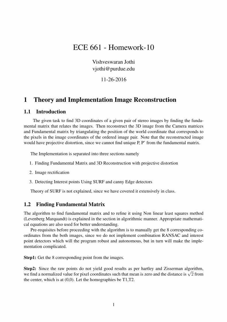
2.6 Canny edges of the Rectified images:

Figure 9: Canny Edge image of Rectified Image1

13

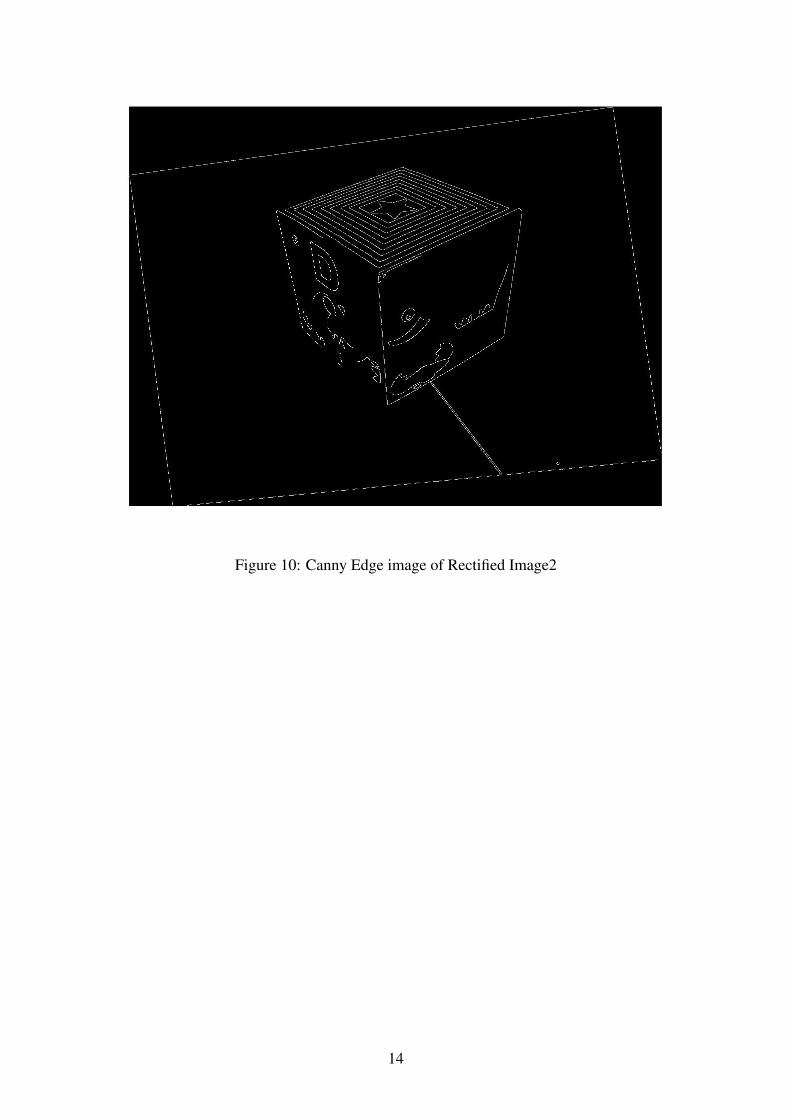
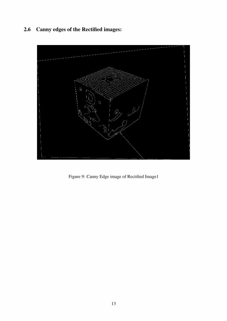
Figure 10: Canny Edge image of Rectified Image2

14

2.7 3D Reconstruction plot from Stereo Images using Canny Edge detector:

Figure 11: 3D reconstruction based on Canny Edge Detection

3 Source Code

3.1 Main function%% Main Programclose all; clear;% Input from the user%path_prompt=’Enter the path where the image pair is located:’;%ext_prompt=’Enter the extension of the image pair:’;%path=input(path_prompt);%ext=input(ext_prompt);path=’/home/vishwa/661/HW10/HW10Pics/’;ext=’*.jpg’;%ext=’*.png’;dest_path=’/home/vishwa/661/HW10/HW10Sourcecode/’;t=0.001;%% Load the manually taken corresponding points on both

15

images and estimate% F matrix, the (x,y) are in vector form

% % house% points_img1=[54,20;37,90;60,158.3;137,226;193,131.65;209,79;174,44;145.65,127];% points_img2=[40.65,36.3;46.35,94.65;72,157;123.65,223.65;208,132.65;223,72.65;182,38.65;104.65,127.3];

% Book% points_img1=[147,236;246,132;118,207.35;113.35,231.65;30.65,115;14.35,79;60.65,51;241.75,171.75];% points_img2=[140.35,235.65;245.35,133;112,205.35;113.35,230;28.35,113;14.65,78.35;60.65,46.35;245,170.65];

% My image 2 - cardboard-1% points_img1=[318.7,160.65;317.35,282.65;396.7,355.35;414.7,231.35;506.7,296.47;526,180;427.35,122.65;413.35,188];% points_img2=[280,178.25;282,300;394,360;412,240.55;471.4,277.7;490.85,164;367.4,115.4;392,193.15];

% % My image 3 - cardboard-1% points_img1=[541.35,320.7;571,667.5;891.35,932.75;920.65,596.55;1196.55,684.5;1310.35,324.15;925.85,120.7;882.75,267.25];% points_img2=[575.85,263.8;601.7,641.4;770.65,965.5;772.4,586.2;1220.65,818.95;1337.9,424.15;1051.7,167.25;924.1,284.5];

% My image 4 - Boxpoints_img1=[451.7,279.3;482.75,700;798.25,987.95;843.1,529.3;1139.65,753.45;1244.8,337.95;850,150;951.7,305.2];points_img2=[486.2,201.6;520.65,619;758.6,922.4;789.7,469;1165.5,730;1272.4,307;922.4,98.3;974.1,257];

g_ssd=5;T_ssd=0.6;surf_ip=1;% Loading the imagesfiles=dir(strcat(path,ext));

for loop=1:length(files)img{loop}=imread(strcat(path,files(loop).name));

end

% Plot the imput images

16

name=’points_coord.jpg’;plot2Dpoints(img{1},img{2},points_img1,points_img2,dest_path,name);

%% Initial estimation of F% Now normalize the input points[pointn_1,T1]=NormalizedH(points_img1);[pointn_2,T2]=NormalizedH(points_img2);% Estimating initial FF_init=computeF(pointn_1,pointn_2,T1,T2);

% Remove the outlier[points_img1,points_img2]=inlier(F_init,points_img1,points_img2,t);% finetuning F w.r. to P’ since P has 11 DOF (12 butwe set the last one to unity)% while F has 7 DOF but has 9 elements in it, weoptimize w.r.to P matrix% thus it does not generate a wrong result.[P2,F_est,X1]=nlsqF(points_img1,points_img2,F_init);e=null(F_est)ep=null(F_est’)% Rectify the images using the optimized F matrix[imrect1,imrect2,F,pts1,pts2,H1,H2]=Img_Rect(points_img1,points_img2,img{1},img{2},F_est);

%% Using Surf interest point detector find Interest pointsand descriptors% Also use canny edge detector to find the interestpoints - Bonus part%Img1_gray=rgb2gray(imrect1);%Img2_gray=rgb2gray(imrect2);if (surf_ip==1)

[points1,points2]=findCorres(imrect1,imrect2,T_ssd,g_ssd);

end

figure;imshow([imrect1 imrect2]); hold on;points1=[points1(2:end,:);pts1’];points2=[points2(2:end,:);pts2’];

for loop=1: length(points1)points=[points1(loop,:);points2(loop,:)+[size(imrect1,2),0]];plot(points1(loop,1),points1(loop,2),’yo’,’MarkerSize’,3,’MarkerFaceColor’,’y’);fig2=plot(points2(loop,1)+size(imrect1,2),

17

points2(loop,2),’yo’,’MarkerSize’,3,’MarkerFaceColor’,’y’);fig2=plot(points(:,1),points(:,2),’-r’,’linewidth’,2);

end

hold off;name=’surf_points2.jpg’;saveas(fig2,strcat(dest_path,name));close all;

% % Finding and optimizing F for new points found using SURF[pointn_1,T1]=NormalizedH(points1);[pointn_2,T2]=NormalizedH(points2);% % Estimating initial FF_init=computeF(pointn_1,pointn_2,T1,T2);[points1,points2]=inlier(F_init,points1,points2,t);epi=null(F_init’);epxi=[0,-epi(3),epi(2);epi(3),0,-epi(1);-epi(2),epi(1),0];P2=[epxi*F_init,epi];% finetuning F w.r. to P’ since P has 11 DOF (12 but we setthe last one to unity)% while F has 7 DOF but has 9 elements in it, we optimizew.r.to P matrix% thus it does not generate a wrong result.

[P2,F_est,X]=nlsqF(points1,points2,F_init);P2=P2; %./P2(end,end);X=triang(points1,points2,P2);X=X(:,2:end);

% Finally plotting the 3D world pointsfname=’3Dfinal.jpg’;plot3Dpoints(X,dest_path,fname);

%% Using Canny edge detector[points1,points2]=findCannycorres(imrect1,imrect2,T_ssd,g_ssd);figure;imshow([imrect1 imrect2]); hold on;points1=[points1(2:end,:);pts1’];points2=[points2(2:end,:);pts2’];for loop=1: length(points1)

points=[points1(loop,:);points2(loop,:)+[size(imrect1,2),0]];plot(points1(loop,1),points1(loop,2),’yo’,’MarkerSize’,3,’MarkerFaceColor’,’y’);fig2=plot(points2(loop,1)+size(imrect1,2),points2(loop,2),

18

’yo’,’MarkerSize’,3,’MarkerFaceColor’,’y’);fig2=plot(points(:,1),points(:,2),’-r’,’linewidth’,2);

end

hold off;name=’canny1.jpg’;saveas(fig2,strcat(dest_path,name));close all;

% Finding and optimizing F for new points found using SURF[pointn_1,T1]=NormalizedH(points1);[pointn_2,T2]=NormalizedH(points2);% Estimating initial FF_init=computeF(pointn_1,pointn_2,T1,T2);[points1,points2]=inlier(F_init,points1,points2,t);epi=null(F_init’);epxi=[0,-epi(3),epi(2);epi(3),0,-epi(1);-epi(2),epi(1),0];P2=[epxi*F_init,epi];% finetuning F w.r. to P’ since P has 11 DOF (12 but we setthe last one to unity)% while F has 7 DOF but has 9 elements in it, we optimizew.r.to P matrix% thus it does not generate a wrong result.

[P2,F_est,X]=nlsqF(points1,points2,F_init);P2=P2; %./P2(end,end);X=triang(points1,points2,P2);

% Finally plotting the 3D world pointsfname=’3Dfinalcanny.jpg’;plot3Dpoints(X,dest_path,fname);

3.2 BiLin%% Function to implement bilinear interpolationfunction[pixel_val]=BiLin(temp_coords,img)tp_lt=img(floor(temp_coords(2)),floor(temp_coords(1)),:);tp_rt=img(floor(temp_coords(2)),floor(temp_coords(1))+1,:);bt_lt=img(floor(temp_coords(2))+1,floor(temp_coords(1)),:);bt_rt=img(floor(temp_coords(2))+1,floor(temp_coords(1))+1,:);del_u=temp_coords(2)-floor(temp_coords(2));del_v=temp_coords(1)-floor(temp_coords(1));pixel_val=(1-del_u)*(1-del_v)*tp_lt+(1-del_v)*del_u*tp_rt...

+(1-del_u)*del_v*bt_lt+del_u*del_v*bt_rt;end

19

3.3 CannyEdge% Function to implement canny edge detectorfunction [eg]=cannyedge(Im)% Converting Image into gray scaleimg=rgb2gray(Im);eg=edge(img,’canny’,0.26);figure;imshow(eg);end

3.4 ComputeF%% Function to Compute F matrixfunction F_init=computeF(points1,points2,T1,T2)row=length(points1);points1=points1’;points2=points2’;% generate the A matrix to compute Af=0Mat=[];for i=1:rowMat=[Mat;points2(i,1)*points1(i,1), points2(i,1)*points1(i,2), points2(i,1),...

points2(i,2)*points1(i,1), points2(i,2)*points1(i,2), points2(i,2),...points1(i,1),points1(i,2),1];

end% use svd to find the right eigen vector to find F matrix[U,D,V]=svd(Mat);Fvec=V(:,end);% since it reshapes column wiseF=reshape(Fvec,3,3);F=F’;% Now condition the F matrix[U1,D1,V1]=svd(F);D1(end,end)=0;F=U1*D1*V1’;F_init= T2’*F*T1;end

3.5 errfunc%% Generating error function to optimise F usingLM algorithmfunction error=errfunc(p,points1,points2)%Pp=[p(1),p(4),p(7),p(10);];Pp=reshape(p(1:12),3,4);%Pp(3,4)=1;%ep=null(f’);P=[eye(3),[0;0;0]];

20

% To get the X world from the parameter vector (p)cnt=13;X=[];for loop=1:((length(p)-12)/3)X=[X,p(cnt:cnt+2)];cnt=cnt+3;endpoints1=[points1’;ones(1,length(points1))];points2=[points2’;ones(1,length(points2))];X=[X;ones(1,length(X))];points1_proj=P*X;points2_proj=Pp*X;points1_proj=[points1_proj(1,:)./points1_proj(3,:);points1_proj(2,:)./points1_proj(3,:);points1_proj(3,:)./points1_proj(3,:);];points2_proj=[points2_proj(1,:)./points2_proj(3,:);points2_proj(2,:)./points2_proj(3,:);points2_proj(3,:)./points2_proj(3,:);];dif=(points1-points1_proj).ˆ2;sum_dif1=dif(1,:)+dif(2,:)+dif(3,:);dif2=(points2-points2_proj).ˆ2;sum_dif2=dif2(1,:)+dif2(2,:)+dif2(3,:);error=sum(sum_dif1(:))+sum(sum_dif2(:));end

3.6 findCannycorres%% Function to implement canny edge detector

function[points1,points2]=findCannycorres(imrect1,imrect2,T_ssd,g_ssd)% Initializing the pointspoint1=[];point2=[];% Finding the edge of theimageedg_1 = cannyedge(imrect1);edg_2 = cannyedge(imrect2);size(edg_1)for i=100:706

for j=270:964if(edg_1(i,j)==1)

point1=[point1;[j,i]];end

endendfor i=147:633

for j=332:901if(edg_2(i,j)==1)

21

point2=[point2;[j,i]];end

endend% set the window size to 24W=24;% choosing 5000 points randomlyidx1 = randperm(5000);point1=point1(idx1,:);point2=point2(idx1,:);% finding descriptor to each imageim1_g=rgb2gray(imrect1);im2_g=rgb2gray(imrect2);[point1,descriptor1]=findDescriptor(point1,im1_g,W);[point2,descriptor2]=findDescriptor(point2,im2_g,W);

% Using SSD to find the best feature match%[points1,points2,˜]=SSD(point1,point2,descriptor1,descriptor2,T_ssd,g_ssd);[points1,points2,˜]=NCC(point1,point2,descriptor1,descriptor2,T_ssd,g_ssd);end

3.7 findCorres%% Finding correspondence for the given imagesfunction [points1,points2]=findCorres(imrect1,imrect2,thresh1,thresh2)

if(length(imrect1(1,1,:))>1)Img1_gray=rgb2gray(imrect1);Img2_gray=rgb2gray(imrect2);else% Img1_gray=imrect1;% Img2_gray=imrect2;endpts1 = detectSURFFeatures(Img1_gray,’MetricThreshold’, 2000);pts2 = detectSURFFeatures(Img2_gray,’MetricThreshold’, 2000);

% pts1 = pts1.selectStrongest(250);% pts2 = pts2.selectStrongest(250);

[features1,validpoints1]=extractFeatures(Img1_gray,pts1);[features2,validpoints2]=extractFeatures(Img2_gray,pts2);

% % Finding matches using SSDpoints1=matchedPoints1.Location;

22

points2=matchedPoints2.Location;[points1,points2,id]=SSD(validpoints1.Location,validpoints2.Location,features1,features2,thresh1,thresh2);

end

3.8 findDescriptor% Function to get the descriptorfunction [points,descriptor]=findDescriptor(point,img,W)% swapping the x,y coordinates to row,col coordinatesfor ease of% computationtemp=[point(:,2),point(:,1)];point=temp;points=[];% initializing descriptordescriptor=zeros(length(point),(W+1)ˆ2);w=W/2;for loop=1:length(point)

if(point(loop,1)-w>1 || point(loop,1)+w<size(img,1)...

||point(loop,2)-w>1 ||point(loop,2)+w<size(img,2))

tmp=img(point(loop,1)-w:point(loop,1)+w,point(loop,2)-w:point(loop,2)+w);descriptor(loop,:)=(tmp(:))’;points=[points;[point(loop,2),point(loop,1)]];end

end

end

3.9 HomographyRect%% Code for to get new homography and apply it torectify the imagefunction[imrect, H_n]=HomographyRect(H,img)img=single(img);[ht,wid,˜]=size(img);

% boundaries of the imageb_pts=[1,1;size(img,2),1;1,size(img,1);size(img,2),size(img,1)];

% New boundary points for the new image planeb_pts_new=H*[b_pts’;ones(1,4)];b_pts_new=[b_pts_new(1,:)./b_pts_new(3,:);b_pts_new(2,:)./b_pts_new(3,:);b_pts_new(3,:)./b_pts_new(3,:)];

23

% Finding the minimum in (x,y) coordinatesmin_val=min(b_pts_new’);max_val=max(b_pts_new’);Dim=(max_val-min_val)’;Dim=[floor(Dim(1));floor(Dim(2))];H_scaling=[wid/Dim(1),0,0;0,ht/Dim(2),0;0,0,1];H=H_scaling*H;% For translationb_pts_new=H*[b_pts’;ones(1,4)];b_pts_new=[b_pts_new(1,:)./b_pts_new(3,:);b_pts_new(2,:)./b_pts_new(3,:);b_pts_new(3,:)./b_pts_new(3,:)];% Finding the minimum in (x,y) coordinatesmin_val=min(b_pts_new’);%max_val=max(b_pts_new’);Dim=min_val’;Dim=[floor(Dim(1));floor(Dim(2))];% generate the offset valuesT=[1,0,-Dim(1)+1;0,1,-Dim(2)+1;0,0,1];% Apply offsets to the Homography functionH_n=T*H;Hinv=inv(H_n);% generate base imageBase=zeros(size(img));for outloop=1:ht

for inloop=1:widtemp_coords=Hinv*[inloop;outloop;1];temp_coords=temp_coords(1:2)./temp_coords(3);if(temp_coords(1)>1 && temp_coords(2)>1 &&temp_coords(1)<wid && temp_coords(2)<ht)

Base(outloop,inloop,:)=BiLin(temp_coords,img);end

endendimrect=uint8(Base);end

3.10 ImgRect%% Rectification of images using Hartley and Zisserman algorithmfunction [imrect1,imrect2,F_rect,pts1,pts2,H1,H2]=Img_Rect(pts_1,pts_2,img1,img2,F)[ht,wid,˜]=size(img1);count=length(pts_1);% points are in column wise after the below stepspts_H1=[pts_1’;ones(1,length(pts_1))];pts_H2=[pts_2’;ones(1,length(pts_2))];e=null(F);ep=null(F’);

24

P=[eye(3),[0;0;0]];epx=[0,-ep(3),ep(2);ep(3),0,-ep(1);-ep(2),ep(1),0];Pp=[epx*F,ep];% making epipolar prime (ep) into the form (x,y,1)ep=ep/ep(3);e=e/e(3);ang=atan(-(ep(2)-ht/2)/(ep(1)-wid/2));f=cos(ang)*(ep(1)-wid/2)-sin(ang)*(ep(2)-ht/2);R=[cos(ang),-sin(ang),0;sin(ang),cos(ang),0; 0,0,1];T=[1,0,-wid/2;0,1,-ht/2;0,0,1];G=[1,0,0;0,1,0;-1/f,0,1];H2=G*R*T;

% keeping the center point in the image as constantc_pt=[wid/2;ht/2;1];c_pt_new=H2*c_pt;c_pt_new=c_pt_new/c_pt_new(3);T2=[1,0,wid/2-c_pt_new(1);0,1,ht/2-c_pt_new(2);0,0,1];H2=T2*H2;

% For H1ang=atan(-(e(2)-ht/2)/(e(1)-wid/2));f=cos(ang)*(e(1)-wid/2)-sin(ang)*(e(2)-ht/2);R=[cos(ang),-sin(ang),0;sin(ang),cos(ang),0; 0,0,1];T=[1,0,-wid/2;0,1,-ht/2;0,0,1];G=[1,0,0;0,1,0;-1/f,0,1];H1=G*R*T;

% keeping the center point in the image as constantc_pt=[wid/2;ht/2;1];c_pt_new=H1*c_pt;c_pt_new=c_pt_new/c_pt_new(3);T1=[1,0,wid/2-c_pt_new(1);0,1,ht/2-c_pt_new(2);0,0,1];H1=T1*H1;

% % Finding Homography for the first image by findingmin a,b,c% M=Pp*pinv(P);% rank(M);% if(rank(M)==2)% %M=[Pp(:,1),Pp(:,3:4)];% end% H0=H2*M;%% pts1_cap=ones(size(pts_H1));% pts2_cap=ones(size(pts_H2));% pts1_cap=H0*pts1_cap;

25

% pts2_cap=H2*pts2_cap;% pts1_cap=[pts1_cap(1,:)./pts1_cap(3,:);pts1_cap(2,:)./pts1_cap(3,:);pts1_cap(3,:)./pts1_cap(3,:)];% pts2_cap=[pts2_cap(1,:)./pts2_cap(3,:);pts2_cap(2,:)./pts2_cap(3,:);pts2_cap(3,:)./pts2_cap(3,:)];%% % Find Ha matrix to get a,b,c values usingLinear Least squares% abc=pinv(pts1_cap’)*(pts2_cap(1,:))’;% Ha=[abc(1),abc(2),abc(3);0,1,0;0,0,1];% H1=Ha*H0;%% % To preserve the center after applying homography% c_pt=[wid/2;ht/2;1];% c_pt_new=H1*c_pt;% c_pt_new=c_pt_new/c_pt_new(3);% T1=[1,0,wid/2-c_pt_new(1);0,1,ht/2-c_pt_new(2);0,0,1];% H1=T1*H1;

% apply the homography to the fundamental matrix andthe image coordinates% such that the epipolar lines go to infinity along x axis[imrect1, H1]=HomographyRect(H1,img1);[imrect2, H2]=HomographyRect(H2,img2);F_rect=inv(H2’)*F*inv(H1);

% The coordinate points on the new plane is given bypts1=zeros(size(pts_1,2),size(pts_1,1));pts2=zeros(size(pts_2,2),size(pts_2,1));tmp_pts1=H1*pts_H1;tmp_pts2=H2*pts_H2;pts1=[tmp_pts1(1,:)./tmp_pts1(3,:);tmp_pts1(2,:)./tmp_pts1(3,:)];pts2=[tmp_pts2(1,:)./tmp_pts2(3,:);tmp_pts2(2,:)./tmp_pts2(3,:)];end

3.11 Inlier% Function to remove the outliersfunction [pts1,pts2]=inlier(F_init,points_img1,points_img2,t);pts1=[];pts2=[];points_img1=[points_img1,ones(length(points_img1),1)];points_img2=[points_img2,ones(length(points_img2),1)];

% if the X2’Fx1< threshold then they pass else they failfor loop=1:length(points_img1)

26

if (points_img2(loop,:)*F_init*(points_img1(loop,:))’<=t)pts1=[pts1;points_img1(loop,1:2)];pts2=[pts2;points_img2(loop,1:2)];

endendend

3.12 nlsqF%% Finding optimized F using Lm optimizationfunction[P2,F_est,X]=nlsqF(points1,points2,F)%points1=points1’;%points2=points2’;% initializing the parameter vectorpoints1=double(points1);points2=double(points2);p=zeros(12+length(points1)*3,1);% Finding the initial e’ using estimated F.epi=null(F’);ep=null(F);% Finding [e’]xepxi=[0,-epi(3),epi(2);epi(3),0,-epi(1);-epi(2),epi(1),0];% Finding initial P’ to pass into the error function to optimize the% parameter vectorP=[eye(3),[0;0;0]];Pp=[epxi*F,epi];%Pp=Pp./Pp(end,end);X=[];for i=1:size(points1,1)

A=[points1(i,1)*P(3,:)-P(1,:);points1(i,2)*P(3,:)-P(2,:);...

points2(i,1)*Pp(3,:)-Pp(1,:);points2(i,2)*Pp(3,:)-Pp(2,:)];[U,D,V]=svd(A);X=[X,V(:,end)/V(end,end)];

endp(1:12)=reshape(Pp,12,1);X_vec=reshape(X(1:3,:),length(points1)*3,1);p(13:end)=X_vec;error=errfunc(p,points1,points2);options=optimoptions(’lsqnonlin’,’Algorithm’,’levenberg-marquardt’,’MaxIter’,10000);p_new=lsqnonlin(@errfunc,p,[],[],options,points1,points2);error1=errfunc(p_new,points1,points2);Pp=reshape(p_new(1:12),3,4);%Pp=Pp./Pp(end,end);ep=Pp(:,4);epx=[0,-ep(3),ep(2);ep(3),0,-ep(1);-ep(2),ep(1),0];F_est=epx*Pp(:,1:3);

27

P2=Pp;% To get the X world optimizedcnt=13;X=[];for loop=1:(length(p_new)-12)/3X=[X;p_new(cnt:cnt+2)’];cnt=cnt+3;endX=X’;end

3.13 NormalizedH%% Function to find the normalized matrix and to normalizethe points using itfunction [points_norm, T]=NormalizedH(points)% points are arranged as per rowspoints=points’;mean_x=mean(points(1,:));mean_y=mean(points(2,:));% finding the distance between mean and the pointstemp=[mean_x;mean_y];mean_mat=repmat(temp,1,length(points));dist_temp=(points-mean_mat).ˆ2;dist=(dist_temp(1,:)+dist_temp(2,:)).ˆ0.5;mean_dist=sum(dist)/length(points);% Setting mean distance as sqrt(2)scale=(2ˆ0.5)/mean_dist;% The below x, y makes zero mean for the pointsx=-scale*mean_x;y=-scale*mean_y;% finally the Transformation matrix is given byT=[scale, 0,x;0,scale,y;0,0,1];points_norm=T*[points;ones(1,size(points,2))];end

3.14 Plot2Dpoints%% Plot 2D points on imagefunction []= plot2Dpoints(img1,img2,points1,points2,dest_path,name)[height,width,˜]=size(img1);% concatenating both the imagesimg=[img1 img2];

imshow(img);hold on;points2_c=points2+repmat([width,0],length(points2),1);

28

for loop=1:length(points2)points=[points1(loop,1),points1(loop,2);points2_c(loop,1),points2_c(loop,2)];fig=plot(points(:,1),points(:,2),’r-’,’linewidth’,1);fig=plot(points1(loop,1),points1(loop,2),’yo’,’MarkerSize’,3,’MarkerFaceColor’,’y’);fig=plot(points2_c(loop,1),points2_c(loop,2),’yo’,’MarkerSize’,3,’MarkerFaceColor’,’y’);endhold off;saveas(fig,strcat(dest_path,name));close all;

end

3.15 Plot3Dpoints%% Function for plotting the 3D world pointsfunction []=plot3Dpoints(X,dest_path,fname)figure;X=X’;hold on;scatter3(X(:,1),X(:,2),X(:,3),’ob’,’Linewidth’,2);cnt=length(X)-7;pt_line=X(cnt:end,:);

for loop=1:3plot3([pt_line(loop,1);pt_line(loop+1,1)],[pt_line(loop,2);pt_line(loop+1,2)],[pt_line(loop,3);pt_line(loop+1,3)],’-r’,’linewidth’,2);endplot3([pt_line(1,1);pt_line(4,1)],[pt_line(1,2);pt_line(4,2)],[pt_line(1,3);pt_line(4,3)],’-r’,’linewidth’,2);plot3([pt_line(3,1);pt_line(5,1)],[pt_line(3,2);pt_line(5,2)],[pt_line(3,3);pt_line(5,3)],’-r’,’linewidth’,2);plot3([pt_line(6,1);pt_line(5,1)],[pt_line(6,2);pt_line(5,2)],[pt_line(6,3);pt_line(5,3)],’-r’,’linewidth’,2);plot3([pt_line(6,1);pt_line(7,1)],[pt_line(6,2);pt_line(7,2)],[pt_line(6,3);pt_line(7,3)],’-r’,’linewidth’,2);plot3([pt_line(6,1);pt_line(4,1)],[pt_line(6,2);pt_line(4,2)],[pt_line(6,3);pt_line(4,3)],’-r’,’linewidth’,2);plot3([pt_line(1,1);pt_line(7,1)],[pt_line(1,2);pt_line(7,2)],[pt_line(1,3);pt_line(7,3)],’-r’,’linewidth’,2);% fig=plot3([pt_line(1,1);pt_line(7,1)],[pt_line(1,2);pt_line(7,2)],[pt_line(1,3);pt_line(7,3)],’-r’,’linewidth’,2);hold off;saveas(fig,strcat(dest_path,fname));

end

29

3.16 SSD% Function for finding SSDfunction [points1,points2,id]=SSD(validpoints1,validpoints2,features1,features2,lt,gt)points1=[];points2=[];points1f=[];points2f=[];SSD_mat=zeros(length(validpoints1),length(validpoints2));for oloop=1:length(validpoints1)

for iloop=1:length(validpoints2)

SSD_mat(oloop,iloop)=sum((features1(oloop,:)-features2(iloop,:)).ˆ2);

endend% Finding global meang_mean=mean(SSD_mat(:));for oloop=1:length(validpoints1)

% Finding minimum value of that rowmin1=min(SSD_mat(oloop,:));% check with global threshold if it passes look for local thresholdif (min1<=gt*g_mean)

[˜,idx]=min(SSD_mat(oloop,:));SSD_mat(oloop,idx)=25000;min2=min(SSD_mat(oloop,:));if (min1/min2 < lt)

points1=[points1;validpoints1(oloop,:)];points2=[points2;validpoints2(idx,:)];SSD_mat(:,idx)=25000*g_mean;

endelse

continue;end

end% Finding if matches are within limitsid=[];

for loop=1:length(points1)if(points1(loop,2)-points2(loop,2)<=25)

id=[id;loop];points1f=[points1f;points1(loop,:)];points2f=[points2f;points2(loop,:)];

endendend

30

3.17 NCC% Function for finding SSDfunction [points1,points2,id]=NCC(validpoints1,validpoints2,features1,features2,lt,gt)points1=[];points2=[];points1f=[];points2f=[];SSD_mat=zeros(length(validpoints1),length(validpoints2));gt=0.7;features1=double(features1);features2=double(features2);for oloop=1:length(validpoints1)

for iloop=1:length(validpoints2)tmp1=(features1(oloop,:)-mean(features1(oloop,:)));tmp2=(features2(iloop,:)-mean(features2(iloop,:)));den=sqrt(sum(tmp1.ˆ2)*sum(tmp2.ˆ2));num=tmp1*tmp2’;SSD_mat(oloop,iloop)=num/den;

endend% Finding global meang_max=max(SSD_mat(:));for oloop=1:length(validpoints1)

% Finding minimum value of that rowmax1=max(SSD_mat(oloop,:));% check with global threshold if it passes lookfor local thresholdif (max1>=gt*g_max)

[˜,idx]=max(SSD_mat(oloop,:));SSD_mat(oloop,idx)=0;max2=max(SSD_mat(oloop,:));if (max2/max1 < lt)

points1=[points1;validpoints1(oloop,:)];points2=[points2;validpoints2(idx,:)];SSD_mat(:,idx)=0;

endelse

continue;end

end% Finding if matches are within limitsid=[];

for loop=1:length(points1)if(points1(loop,2)-points2(loop,2)<=25)

id=[id;loop];

31

points1f=[points1f;points1(loop,:)];points2f=[points2f;points2(loop,:)];

endendend

3.18 triang% Function for triangulationfunction[X]=triang(points1,points2,P2)P=[eye(3),[0;0;0]];Pp=P2;X=[];for i=1:size(points1,1)

A=[points1(i,1)*P(3,:)-P(1,:);points1(i,2)*P(3,:)-P(2,:);...

points2(i,1)*Pp(3,:)-Pp(1,:);points2(i,2)*Pp(3,:)-Pp(2,:)];

[U,D,V]=svd(A);X=[X,V(:,end)/V(end,end)];

endend

This is the end of the document.

32