ECE 662 Spring 2008 Homework 2 Report - Project Rhea ... · ECE 662 Spring 2008 Homework 2 Report ... we have used a real dataset titled 'Pen-Based Recognition of Handwritten Digits'

ECE 662 Spring 2008

Homework 2 Report

April 16, 2008

1 Problem 1

In the Parametric Method section of the course, we learned how to draw a separation hyperplane

between two classes by obtaining wopt, the argmax of the cost function J(w) = wT SBw

wT SW w. The

solution was found to be wopt = S−1W (m1 − m2), where m1 and m2 are the sample means of each

class, respectively. Some students raised the question: can one simply use J(w) = wT SBw instead

(i.e. setting SW as the identity matrix in the solution wopt)? Investigate this question by numericalexperimentation.

1.1 Methodology

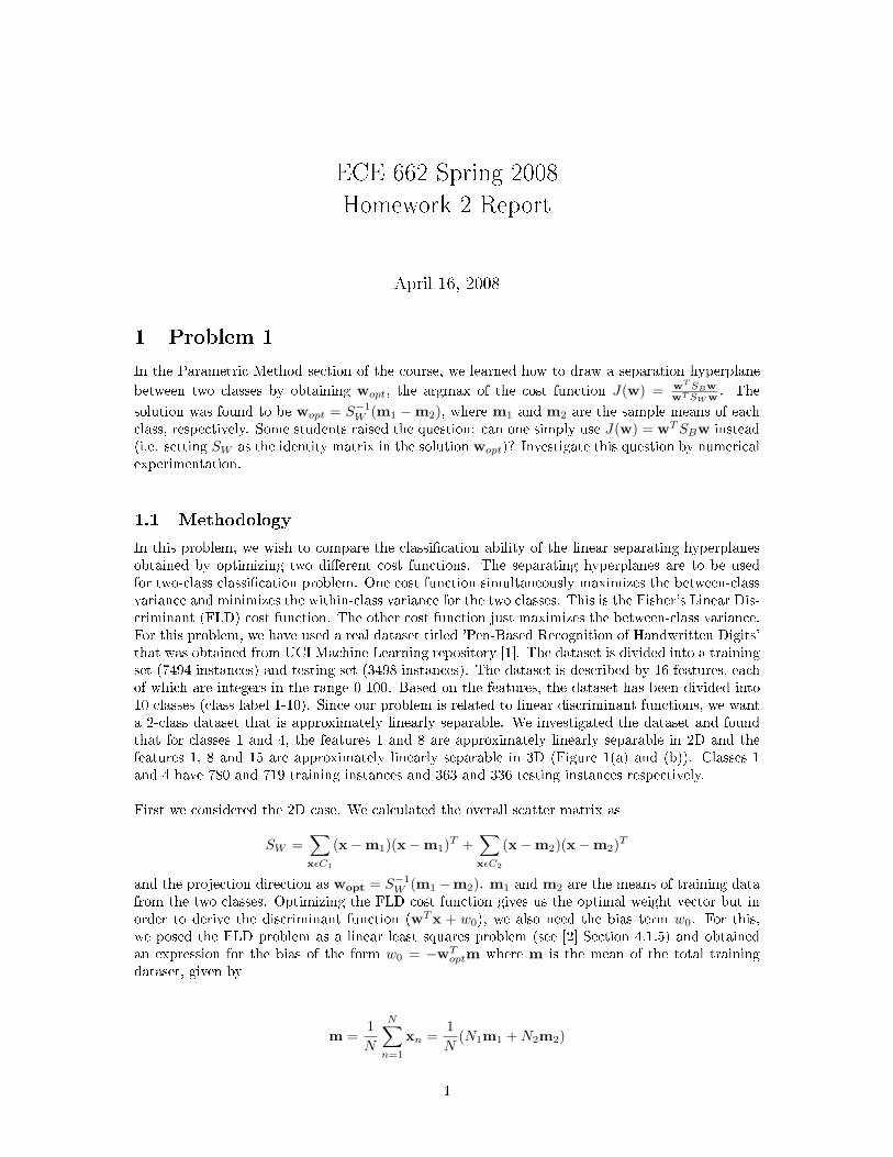
In this problem, we wish to compare the classi�cation ability of the linear separating hyperplanesobtained by optimizing two di�erent cost functions. The separating hyperplanes are to be usedfor two-class classi�cation problem. One cost function simultaneously maximizes the between-classvariance and minimizes the within-class variance for the two classes. This is the Fisher's Linear Dis-criminant (FLD) cost function. The other cost function just maximizes the between-class variance.For this problem, we have used a real dataset titled 'Pen-Based Recognition of Handwritten Digits'that was obtained from UCI Machine Learning repository [1]. The dataset is divided into a trainingset (7494 instances) and testing set (3498 instances). The dataset is described by 16 features, eachof which are integers in the range 0-100. Based on the features, the dataset has been divided into10 classes (class label 1-10). Since our problem is related to linear discriminant functions, we wanta 2-class dataset that is approximately linearly separable. We investigated the dataset and foundthat for classes 1 and 4, the features 1 and 8 are approximately linearly separable in 2D and thefeatures 1, 8 and 15 are approximately linearly separable in 3D (Figure 1(a) and (b)). Classes 1and 4 have 780 and 719 training instances and 363 and 336 testing instances respectively.

First we considered the 2D case. We calculated the overall scatter matrix as

SW =∑

xǫC1

(x − m1)(x − m1)T +

∑

xǫC2

(x − m2)(x − m2)T

and the projection direction as wopt = S−1W (m1 −m2). m1 and m2 are the means of training data

from the two classes. Optimizing the FLD cost function gives us the optimal weight vector but inorder to derive the discriminant function (wT

x + w0), we also need the bias term w0. For this,we posed the FLD problem as a linear least squares problem (see [2] Section 4.1.5) and obtainedan expression for the bias of the form w0 = −w

Toptm where m is the mean of the total training

dataset, given by

m =1

N

N∑

n=1

xn =1

N(N1m1 + N2m2)

1

1.2 Results and Discussion

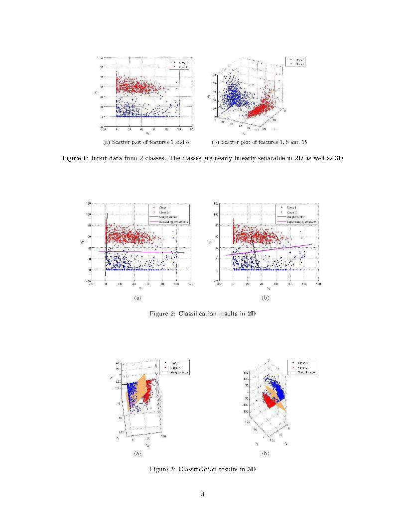
Figure 2(a) shows the wopt (black line) and the separating hyperplane (magenta line) that are ob-tained by optimizing the FLD cost function. From the �gure, it is apparent that this wopt is infacta good choice for maximizing the between-class variance and minimizing the within-class scatterfor the two classes. When we do not include the within-class scatter in the cost function, we aree�ectively setting SW to identity matrix and in this case, wopt is simply (m1−m2) i.e. the optimalweight vector is along the line joining the two class means. For this case, the weight vector wopt

and the separating hyperplane are shown in Figure 2(b). We refer to these as di�erence-of-meanweight vector and di�erence-of-mean hyperplane. From the �gure, we can tell that in general theseare not the best choices for the optimal weight vector and the separating hyperplane.

Interestingly enough, when we used these hyperplanes to classify the test data from the two classes,the results were a little counter intuitive. The di�erence-of-mean hyperplane performed slightly bet-ter than the FLD hyperplane. The numerical results are summarized in table 1. We had anticipatedthat FLD classi�er will perform better than the di�erence-of-means classi�er. The unexpected re-sult may be due to the particular distributions of the two classes. We can de�nitely construct twoclass distributions where the FLD classi�er performs better than the di�erence-of-means classi�er.We demonstrate such a case later in our report. For right now, we proceed with discussing theperformance comparison between the two classi�ers on 3D dataset.

For the 3D case, we obtain wopt and w0 for both types of classi�ers, similarly to the 2D case.Figures 3 (a) and (b) show the weight vector wopt and the separating hyperplanes for the twoclassi�ers. In 3D also, the di�erence-of-means classi�er performs better than the FLD classi�er asis apparent from table 2.

A little earlier in our report, we had commented that in general we expect FLD classi�er to performsuperior to the di�erence-of-means classi�er. The reason is that FLD cost function simultaneouslyoptimizes two di�erent criteria (maximize between-class variance and minimize within-class vari-ance) which is more logical. But there may be some data distributions for which the latter performsbetter. This is precisely the case with our selected real dataset. On the other hand, we can showthat there exist data distributions for which FLD classi�er will perform better. One such exampleis shown in �gure 4(a) and (b), where we have shown the FLD classi�er and di�erence-of-meanclassi�er results for 2 class Gaussian distributions. The means of the Gaussian distributions arehorizontally displaced from each other and their axes of maximum variance are parallel to each otherand inclined at an angle with the horizontal. From the numbers in table 3, we observes that FLDgives perfect classi�cation (100% accuracy) for this dataset while di�erence-of-mean classi�er yields95.8% accuracy. From this exercise, we learned a good lesson that it is better to use real life

datasets to gauge the performance of di�erent classi�ers because an arti�cial dataset

can always be generated to con�rm the preconceptions that we may have regarding

the relative classi�cation abilities of di�erent techniques.

2

(a) Scatter plot of features 1 and 8 (b) Scatter plot of features 1, 8 and 15

Figure 1: Input data from 2 classes. The classes are nearly linearly separable in 2D as well as 3D

(a) (b)

Figure 2: Classi�cation results in 2D

(a) (b)

Figure 3: Classi�cation results in 3D

3

Fisher's Linear Discriminant Di�erence-of-Means

# Test vectors 699 699# Misclassi�cations 29 22

% Classi�cation Accuracy 95.85 96.85

Table 1: Classi�cation accuracy comparison in 2D



% Classi�cation Accuracy 96.57 98.14

Table 2: Classi�cation accuracy comparison in 3D

(a) (b)

Figure 4: Classi�cation results in 2D for Gaussian class distribution



% Classi�cation Accuracy 100 95.8

Table 3: Classi�cation accuracy comparison in 2D for Gaussian class distribution

4

2 Problem 2

In this problem we had to experiment with designing a classi�er using neural network and supportvector machine approaches and then compare the two.

2.1 Methodology

We considered a 2-class classi�cation problem and used the same two classes as in problem 1. Forthe neural network classi�cation, we used the MATLAB Neural Network toolbox. In particular,we used 3 MATLAB functions: newff, train and sim, whose functionalities are brie�y explainedbelow:

• newff - create the neural network by specifying the number of hidden layers, number ofneurons in each hidden layer and the transfer functions to be used in each layer. The numberof neurons in the output layer is automatically determined from the target vector.

• train - train the neural network using the training data.

• sim - classify the testing data using the trained network.

In our experiments, we designed 3 neural networks. We call them NN1, NN2 and NN3. Wespeci�ed the number of layers as follows:

1. NN1 had 1 hidden layer with 5 neurons and 1 output layer with 1 neuron.

2. NN2 had 2 hidden layers with 5 neurons each and 1 output layer with 1 neuron.

3. NN3 had 3 hidden layers with 5, 10 and 5 neurons respectively and 1 output layer with 1neuron.

Note that each network has only 1 neuron in the output layer since we want the network outputto be class labels which are single integers. The transfer function was chosen as arctan() for thehidden layers and linear for output layer. In our experiments, we were using the class labels '1' and'4'. Since the output of network was a real number for every test vector, we thresholded the outputas:

ClassLabel =

{

1 network output 6 2.5

4 network output > 2.5

Since our dataset has 16 features for the 2 classes, we tried to classify the data with the neural net-work approach by varying the number of features and evaluate which con�guration of the networkand how many features resulted is a good classi�cations accuracy.

For the SVM approach, we used the LIBSVM software v2.85 [3] which is a command line toolfor SVM classi�cation. The source code is available in C++ and Java and the software has inter-faces for MATLAB, R, Python and so on. We used the C++ binaries for running our experiments.The software also comes with 'A Practical Guide to Support Vector Classi�cation' which suggestssome easy but signi�cant steps to get good SVM classi�cation on our data.

In order to understand some of the parameters used in our experiments, we delve brie�y intothe theory behind SVM. The goal of SVM is to produce a model which predicts target value of datainstances in the testing set, when only the features are known. Given a training set of instance-labelpairs (xi, yi), i = 1, . . . , N where xi ∈ Rn and y ∈ {−1, 1}

N, the support vector machines (SVM)

require the solution of the following optimization problem:

5

minw,b,ξ

1

2w

Tw + C

N∑

i=1

ξi

subject to yi

(

wT φ (xi) + b

)

> 1 − ξi

ξi > 0

Here training vectors xi are mapped into a higher (maybe in�nite) dimensional space by thefunction φ. Then SVM �nds a linear separating hyperplane with the maximal margin in thishigher dimensional space. C > 0 is the penalty parameter of the error term. Furthermore,K(xi,xj) = φ(xi)

T φ(xj) is called the kernel function.

The procedure suggested in this software was as follows:

1. Conduct simple scaling of the data. The main advantage is to avoid features in greater numericranges dominate those in smaller numeric ranges. Another advantage is to avoid numericaldi�culties during the calculation. Since all our feature values were integers in the range 0 to100, we scaled that data to 0-1 range.

2. Consider the Radial Basis Function (RBF) kernel K (x,y) = e−γ‖x−y‖2

3. Use cross-validation to �nd the best parameters C and γ

4. Use the best parameters C and γ to train the whole training set

5. Test on the testing data


Table 4 summarizes the numerical classi�cation accuracy percentages for the 3 neural networks whenthe number of features were varied from 1 to 16. In table 5, we present the results of SVM trainingand testing. The software �nds the best values of C and γ and evaluates the 5-fold cross validationaccuracy for training set classi�cation. Then this (C, γ) pair is used on the testing data. Figure 5depicts the performance comparison between the neural network and SVM approaches. From the�gure, we can make several observations. First is that the data is not well separated in the �rst 2dimensions because both neural network and SVM give ∼65% and ∼75% accuracy when using onlythe �rst or �rst two dimensions for classi�cation. Starting from 3 features onwards, both types ofclassi�ers give &96% accuracy. So we do not need to use all 16 features for classi�cation. The �rst3-5 features should be su�cient. We also note that NN1, NN2 and SVM have relatively similarperformances while NN3 performs inferior to them. This suggests that increasing the number ofhidden layers or the number of neurons in a hidden layer may not necessarily improve performance.

6

#Features NN1 NN2 NN3

1 63.23 62.52 61.662 75.54 75.68 74.963 97 98 95.574 95.71 97 95.715 99.71 99.57 89.416 97 99 98.437 99.86 99.57 97.428 98.43 99.57 989 99.71 98.86 98.4310 100 99.86 75.8211 99.86 99.28 98.8612 97.85 96.71 99.8613 99.71 97.85 9814 99.86 98.14 97.8515 99.86 99.86 97.5716 99.28 99 98.57

Table 4: Classi�cation accuracy percentages for Neural Network approach

#Features Best C Best γ Cross Validation Accuracy (%) Accuracy on test data (%)

1 2048 0.5 59.31 63.232 8 8 74.85 75.393 0.13 8 97.87 98.434 8192 0.13 99.6 97.575 2 0.01 99.87 996 0.03 8 99.87 99.577 0.03 8 99.93 99.578 0.03 8 100 99.579 0.03 8 99.93 99.5710 0.5 8 100 99.7111 0.13 2 100 99.8612 0.03 2 100 99.8613 0.03 2 100 99.8614 0.03 2 100 99.8615 0.13 0.01 99.93 97.1416 0.13 0.01 99.93 97.57

Table 5: Classi�cation accuracy for SVM approach

7

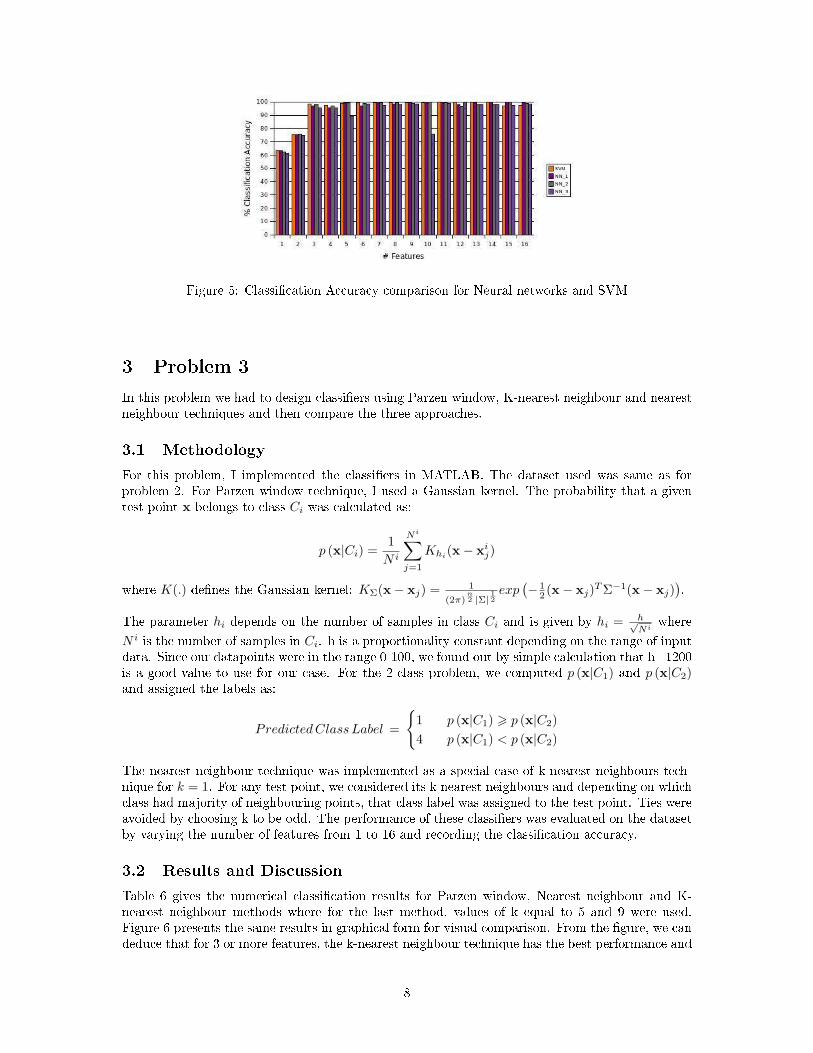
Figure 5: Classi�cation Accuracy comparison for Neural networks and SVM

3 Problem 3

In this problem we had to design classi�ers using Parzen window, K-nearest neighbour and nearestneighbour techniques and then compare the three approaches.

3.1 Methodology

For this problem, I implemented the classi�ers in MATLAB. The dataset used was same as forproblem 2. For Parzen window technique, I used a Gaussian kernel. The probability that a giventest point x belongs to class Ci was calculated as:

p (x|Ci) =1

N i

Ni

∑

j=1

Khi(x − x

ij)

where K(.) de�nes the Gaussian kernel: KΣ(x − xj) = 1

(2π)n

2 |Σ|1

2

exp(

− 12 (x − xj)

T Σ−1(x − xj))

.

The parameter hi depends on the number of samples in class Ci and is given by hi = h√Ni

where

N i is the number of samples in Ci. h is a proportionality constant depending on the range of inputdata. Since our datapoints were in the range 0-100, we found out by simple calculation that h=1200is a good value to use for our case. For the 2-class problem, we computed p (x|C1) and p (x|C2)and assigned the labels as:

PredictedClassLabel =

{

1 p (x|C1) > p (x|C2)

4 p (x|C1) < p (x|C2)

The nearest neighbour technique was implemented as a special case of k-nearest neighbours tech-nique for k = 1. For any test point, we considered its k nearest neighbours and depending on whichclass had majority of neighbouring points, that class label was assigned to the test point. Ties wereavoided by choosing k to be odd. The performance of these classi�ers was evaluated on the datasetby varying the number of features from 1 to 16 and recording the classi�cation accuracy.


Table 6 gives the numerical classi�cation results for Parzen window, Nearest neighbour and K-nearest neighbour methods where for the last method, values of k equal to 5 and 9 were used.Figure 6 presents the same results in graphical form for visual comparison. From the �gure, we candeduce that for 3 or more features, the k-nearest neighbour technique has the best performance and

8

the nearest neighbour technique is closely second to it. Parzen window method consistently performsthe lowest among the three methods. For 1 and 2 features, the two classes are highly overlappingand so it is di�cult to assess the relative performance of the classi�ers using only these two features.

Since we used density estimation for the Parzen window estimator, for demonstration purposes,we present in �gure 7, the estimated densities for the two classes based only on feature 8. Thisfeature was chosen simply to show how the density estimation leads to classi�cation, because thetwo classes were well separated in this feature.

#Features Parzen window Nearest neighbour KNN (k=5) KNN (k=9)

1 56.94 51.93 51.93 51.652 58.94 63.66 71.24 73.253 94.13 97 97.28 96.854 93.42 97.71 97.28 97.145 97.14 99.57 99.57 99.436 96.71 99.57 99.57 99.287 97.71 99.57 99.57 99.578 97.57 99.57 99.57 99.439 98.14 99.57 99.86 99.8610 98.43 99.57 99.71 99.5711 98.43 99.57 99.57 99.5712 98.43 99.57 99.71 99.7113 98.71 99.57 99.71 99.7114 98.43 99.57 99.71 99.7115 99.28 99.71 99.71 99.7116 99.71 99.71 99.86 99.86

Table 6: Classi�cation accuracy percentages for non-parametric techniques

Figure 6: Classi�cation accuracy comparison for Parzen window, nearest neighbour and k-nearestneighbour approaches

9

Figure 7: Density estimation on feature# 8 of the dataset

4 Comparing all the classi�ers

In problem 1, we compared the performance of Fisher's linear discriminant and di�erence-of-meansclassi�ers on 2- and 3-dimensional data which was approximately linearly separable. We performedmore experiments to investigate how do the other classi�ers perform on the same data.

4.1 Methodology

The di�erent classi�ers that were used for this experiment were Fisher's Linear Discriminant,Di�erence-of-Means, Neural Network (1 hidden layer with 5 neurons), SVM, Parzen Window,Nearest Neighbour and k-Nearest Neighbour (k=5,9). Table 7 presents the numerical classi�ca-tion accuracy percentages for these classi�ers, on 2- and 3-dimensional datasets and �gure 8 showsthe same results in graphical form. For the sake of clarity on the �gures, the classi�er names havebeen abbreviated as FLD, DoM,NNET, SV M, NN,KNN5 and KNN9.


From the results, it is obviously clear that the classi�ers resulting in non-linear classi�cation bound-aries (e.g. SVM, Neural network, Parzen window, KNN etc.) perform better than linear classi�ers(Fisher's Linear discriminant and Di�erence-of-Means classi�ers). For the 2-d dataset, SVM andneural network give the best accuracy followed by non-parametric techniques (KNN, Parzen win-dow). On the other hand, for the 3-d dataset, K-nearest neighbour and SVM give practically thebest accuracy and they are followed by nearest neighbour and neural network approaches.

Type of classi�er % classi�cation accuracy (2-d data) % classi�cation accuracy (3-d data)

Fisher's Linear Discriminant 95.85 96.57Di�erence-of-means 96.85 98.14Neural network 98.14 98.14

SVM 98.99 99.33Parzen window 96.28 97.85

Nearest neighbour 96.85 98.57K-nearest neighbour (k=5) 97.85 99.57K-nearest neighbour (k=9) 97.85 99.57

Table 7: All classi�er performance on 2-d and 3-d datasets

10

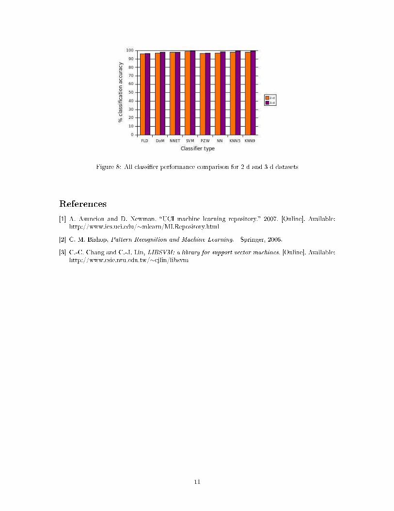
Figure 8: All classi�er performance comparison for 2-d and 3-d datasets

References

[1] A. Asuncion and D. Newman, �UCI machine learning repository,� 2007. [Online]. Available:http://www.ics.uci.edu/∼mlearn/MLRepository.html

[2] C. M. Bishop, Pattern Recognition and Machine Learning. Springer, 2006.

[3] C.-C. Chang and C.-J. Lin, LIBSVM: a library for support vector machines. [Online]. Available:http://www.csie.ntu.edu.tw/∼cjlin/libsvm

11

% ECE 662 HW2 Problem 1 : Linear discriminant classification for 2-d datasetclose all;

global training_data test_data

% Fisher's Linear Discriminant in 2Dclass1_data = [training_data{1,1} training_data{1,8}];class2_data = [training_data{4,1} training_data{4,8}];

figure;hold on;plot(class1_data(:,1),class1_data(:,2),'.');plot(class2_data(:,1),class2_data(:,2),'r.');axis([-20 120 -20 120]);

m1=mean(class1_data);m2=mean(class2_data);

S_W = zeros(2,2);

for i=1:size(class1_data) S_W = S_W + (class1_data(i,:)-m1)'*(class1_data(i,:)-m1);end


% determining optimal weight vectorw = inv(S_W)*((m1-m2))';

% plotting the weight vectorslope = w(2)/w(1);x1=1.8;y1=slope*x1;x2=-.2;y2=slope*x2;plot([x1;x2],[y1;y2],'k-','LineWidth',2);

% for i=1:size(class1_data)% l = (class1_data(i,:)*w)/(w'*w);% plot(l*w(1)-10,l*w(2), 'o');% end% % for i=1:size(class2_data)% l = (class2_data(i,:)*w)/(w'*w);% plot(l*w(1)-10,l*w(2), 'ro');% end

N1=size(class1_data,1);N2=size(class2_data,1);N=N1+N2;

% m is the overall mean of the training datam=(N1*m1+N2*m2)/N;

% This choice of w0 is obtained by posing the Fisher's Linear discriminant% as a least squares problem.w0=-w'*m';

% plotting the discriminating hyperplane

x1=-10;y1=-(w(1)*x1+w0)/w(2);x2=110;y2=-(w(1)*x2+w0)/w(2);plot([x1;x2],[y1;y2],'m-','LineWidth',2);

xlabel('x_1');ylabel('x_2');legend('Class 1','Class 2', 'Weight vector', 'Separating hyperplane');grid on;

% testing the accuracy of the separating hyperplane on test datatesting_data = [[test_data{1,1} test_data{1,8}]; [test_data{4,1} test_data{4,8}]];

N1_test = length(test_data{1,1});N2_test = length(test_data{4,1});true_class_label = [ones(N1_test,1); 2*ones(N2_test,1)];estimated_class_label = zeros(N1_test+N2_test,1);

for i=1:N1_test+N2_test x = testing_data(i,:); if (w'*x'+w0) > 0 estimated_class_label(i) = 1; else estimated_class_label(i) = 2; endend

num_misclassifications = sum(true_class_label ~= estimated_class_label);classification_accuracy = (1-(num_misclassifications/(N1_test+N2_test)))*100;

disp('Classification using FLD weight vector.');disp(['# test vectors: ' num2str(N1_test+N2_test)]);disp(['# misclassifications: ' num2str(num_misclassifications)]);disp(['# classification accuracy: ' num2str(classification_accuracy)]);

% Starting from here, we investigate the effect of setting S_W to identity matrixfigure;hold on;plot(class1_data(:,1),class1_data(:,2),'.');plot(class2_data(:,1),class2_data(:,2),'r.');plot([m1(1);m2(1)],[m1(2);m2(2)],'k-','LineWidth',2);axis([-20 120 -20 120]);

S_W = eye(2);

% determining optimal weight vectorw = inv(S_W)*(m1-m2)';


% plotting the discriminating hyperplanex1=-10;y1=-(w(1)*x1+w0)/w(2);x2=110;y2=-(w(1)*x2+w0)/w(2);plot([x1;x2],[y1;y2],'m-','LineWidth',2);

xlabel('x_1');ylabel('x_2');legend('Class 1','Class 2', 'Weight vector', 'Separating hyperplane');grid on;

% testing the accuracy of the separating hyperplane on test datatesting_data = [[test_data{1,1} test_data{1,8}]; [test_data{4,1} test_data{4,8}]];

N1_test = length(test_data{1,1});N2_test = length(test_data{4,1});true_class_label = [ones(N1_test,1); 2*ones(N2_test,1)];estimated_class_label = zeros(N1_test+N2_test,1);

for i=1:N1_test+N2_test x = testing_data(i,:); if (w'*x'+w0) > 0 estimated_class_label(i) = 1; else estimated_class_label(i) = 2; endend

num_misclassifications = sum(true_class_label ~= estimated_class_label);classification_accuracy = (1-(num_misclassifications/(N1_test+N2_test)))*100;

disp('Classification using difference-of-means weight vector.');disp(['# test vectors: ' num2str(N1_test+N2_test)]);disp(['# misclassifications: ' num2str(num_misclassifications)]);disp(['# classification accuracy: ' num2str(classification_accuracy)]);

% ECE 662 HW2 Problem 1 : Linear discriminant classification for 3-d datasetclose all;

global training_data test_data

% Fisher's Linear Discriminant in 3Dclass1_data = [training_data{1,1} training_data{1,8} training_data{1,15}];class2_data = [training_data{4,1} training_data{4,8} training_data{4,15}];

figure;hold on;plot3(class1_data(:,1),class1_data(:,2),class1_data(:,3),'.');plot3(class2_data(:,1),class2_data(:,2),class2_data(:,3),'r.');

m1=mean(class1_data);m2=mean(class2_data);

S_W = zeros(3,3);



% determining optimal weight vectorw = inv(S_W)*((m1-m2))';

% plotting the weight vectorpoint1 = (5e4)*w;point2 = (-20e4)*w;plot3([point1(1);point2(1)],[point1(2);point2(2)],[point1(3);point2(3)],'k-','LineWidth',2);grid on;

N1=size(class1_data,1);N2=size(class2_data,1);N=N1+N2;

% m is the overall mean of the training datam=(N1*m1+N2*m2)/N;


% plotting the discriminating hyperplane[X,Y]=meshgrid([-5:60]);Z=-(w(1)*X+w(2)*Y+w0)/w(3);surf(X,Y,Z);axis equal;

xlabel('x_1');ylabel('x_2');zlabel('x_3');legend('Class 1','Class 2', 'Weight vector');grid on;

% testing the accuracy of the separating hyperplane on test datatesting_data = [[test_data{1,1} test_data{1,8} test_data{1,15}]; [test_data{4,1} test_data{4,8} test_data{4,15}]];

N1_test = length(test_data{1,1});N2_test = length(test_data{4,1});true_class_label = [ones(N1_test,1); 2*ones(N2_test,1)];FLD_class_label = zeros(N1_test+N2_test,1);

for i=1:N1_test+N2_test x = testing_data(i,:); if (w'*x'+w0) > 0 FLD_class_label(i) = 1; else FLD_class_label(i) = 2; endend

num_misclassifications = sum(true_class_label ~= FLD_class_label);classification_accuracy = (1-(num_misclassifications/(N1_test+N2_test)))*100;

disp('Classification using FLD weight vector.');disp(['# test vectors: ' num2str(N1_test+N2_test)]);disp(['# misclassifications: ' num2str(num_misclassifications)]);

disp(['# classification accuracy: ' num2str(classification_accuracy)]);

% Starting from here, we investigate the effect of setting S_W to identity matrixfigure;hold on;plot3(class1_data(:,1),class1_data(:,2),class1_data(:,3),'.');plot3(class2_data(:,1),class2_data(:,2),class2_data(:,3),'r.');plot3([m1(1);m2(1)],[m1(2);m2(2)],[m1(3);m2(3)],'k-','LineWidth',2);

S_W = eye(3);

% determining optimal weight vectorw = inv(S_W)*(m1-m2)';


% plotting the discriminating hyperplane[X,Y]=meshgrid([-5:60]);Z=-(w(1)*X+w(2)*Y+w0)/w(3);surf(X,Y,Z);axis equal;

xlabel('x_1');ylabel('x_2');legend('Class 1','Class 2', 'Weight vector');grid on;

% testing the accuracy of the separating hyperplane on test datatesting_data = [[test_data{1,1} test_data{1,8} test_data{1,15}]; [test_data{4,1} test_data{4,8} test_data{4,15}]];

N1_test = length(test_data{1,1});N2_test = length(test_data{4,1});true_class_label = [ones(N1_test,1); 2*ones(N2_test,1)];FLD_class_label = zeros(N1_test+N2_test,1);

for i=1:N1_test+N2_test x = testing_data(i,:); if (w'*x'+w0) > 0 FLD_class_label(i) = 1; else FLD_class_label(i) = 2; endend

num_misclassifications = sum(true_class_label ~= FLD_class_label);classification_accuracy = (1-(num_misclassifications/(N1_test+N2_test)))*100;

disp('Classification using difference-of-means weight vector.');disp(['# test vectors: ' num2str(N1_test+N2_test)]);disp(['# misclassifications: ' num2str(num_misclassifications)]);disp(['# classification accuracy: ' num2str(classification_accuracy)]);

% ECE 662 HW 2 Problem 2 : Neural network classification

class1 = 1;class2 = 4;

N1_train = length(training_data{class1,1});N2_train = length(training_data{class2,1});

N1_test = length(test_data{class1,1});N2_test = length(test_data{class2,1});

neural_train_labels = [ones(N1_train,1); 4*ones(N2_train,1)]; neural_test_labels = [ones(N1_test,1); 4*ones(N2_test,1)]; fp=fopen('nn_results.txt','w'); for attribute=1:16 neural_train_data=[]; neural_test_data=[]; % preparing training and test data for j=1:attribute neural_train_data = [neural_train_data [training_data{class1,j};training_data{class2,j}]]; neural_test_data = [neural_test_data [test_data{class1,j};test_data{class2,j}]]; end % creating, training and testing the network. net = newff(neural_train_data', neural_train_labels', 5); net = train(net, neural_train_data', neural_train_labels'); net_output = sim(net, neural_test_data'); % The network output needs to be threholded to give a 2-class % classification. index = find(net_output<=2.5); net_output(index) = 1; index = find(net_output>2.5); net_output(index) = 4; num_misclassifications = sum(neural_test_labels' ~= net_output); classification_accuracy = (1-(num_misclassifications/(N1_test+N2_test)))*100; disp(classification_accuracy); fprintf(fp,'%4.2f\n',classification_accuracy); end

fclose(fp);

% ECE 662 HW 2 Problem 3 : Parzen Window Density Estimation

% We use Gaussian Parzen window.

ATTRIBUTES=16;

N1_train = length(training_data{1,1});N2_train = length(training_data{4,1});N1_test = length(test_data{1,1});N2_test = length(test_data{4,1});

h=1200;h_N1=h/sqrt(N1_train);h_N2=h/sqrt(N2_train);

parzen_train_labels = [ones(N1_train,1); 4*ones(N2_train,1)]; parzen_test_labels = [ones(N1_test,1); 4*ones(N2_test,1)];

for attribute=1:ATTRIBUTES parzen_train_data=[]; parzen_test_data=[];

for j=1:attribute parzen_train_data = [parzen_train_data [training_data{1,j};training_data{4,j}]]; parzen_test_data = [parzen_test_data [test_data{1,j};test_data{4,j}]]; end

predicted_test_labels=[];

for i=1:N1_test+N2_test test_point = parzen_test_data(i,:); test_vector = ones(N1_train+N2_train,1) * test_point;

diff_vector = parzen_train_data - test_vector; diff_vector(1:N1_train,:) = diff_vector(1:N1_train,:)/h_N1; diff_vector(N1_train+1:N1_train+N2_train,:) = diff_vector(N1_train+1:N1_train+N2_train,:)/h_N2; if attribute == 1 gaussian_pdf_values = normpdf(diff_vector); else gaussian_pdf_values = mvnpdf(diff_vector); end class1_probability = sum(gaussian_pdf_values(1:N1_train))/N1_train; class2_probability = sum(gaussian_pdf_values(N1_train+1:N1_train+N2_train))/N2_train;

if class1_probability >= class2_probability predicted_test_labels=[predicted_test_labels;1]; else predicted_test_labels=[predicted_test_labels;4]; end end

num_misclassifications = sum(parzen_test_labels ~= predicted_test_labels); classification_accuracy = 100*(1 - num_misclassifications/(N1_test+N2_test)); disp(['attributes=' num2str(attribute) ' <--> Classification accuracy=' num2str(classification_accuracy) '%']);end

% ECE 662 HW 2 Problem 3 : Nearest neighbour and K-nearest neighbour% algorithm implementation.

K=[1 3 5 7 9];

ATTRIBUTES=16;

N1_train = length(training_data{1,1});N2_train = length(training_data{4,1});N1_test = length(test_data{1,1});N2_test = length(test_data{4,1});

knn_train_labels = [ones(N1_train,1); 4*ones(N2_train,1)]; knn_test_labels = [ones(N1_test,1); 4*ones(N2_test,1)];

fp = fopen('knn_results.txt','w');

for k=K fprintf(fp, 'k=%d\n\n',k); for attribute=1:ATTRIBUTES disp(['k=' num2str(k) ' attributes=' num2str(attribute)]); knn_train_data=[]; knn_test_data=[]; for j=1:attribute knn_train_data = [knn_train_data [training_data{1,j};training_data{4,j}]]; knn_test_data = [knn_test_data [test_data{1,j};test_data{4,j}]]; end predicted_test_labels=[];

for i=1:N1_test+N2_test test_point = knn_test_data(i,:); test_vector = ones(N1_train+N2_train,1) * test_point;

diff_vector = knn_train_data - test_vector; euclidean_distance = sqrt(sum((diff_vector .* diff_vector),2));

[sorted_distance, index]=sort(euclidean_distance);

class1_score=0; class2_score=0;

for m=1:k if knn_train_labels(index(m)) == 1 class1_score=class1_score+1; else class2_score=class2_score+1; end end

if class1_score > class2_score predicted_test_labels=[predicted_test_labels;1]; else predicted_test_labels=[predicted_test_labels;4]; end end num_misclassifications = sum(knn_test_labels ~= predicted_test_labels); classification_accuracy = 100*(1 - num_misclassifications/(N1_test+N2_test)); fprintf(fp, '%4.2f\n', classification_accuracy); end fprintf(fp, '\n\n');end

fclose(fp);

ECE 662 Spring 2008 Homework 2 Report - Project Rhea ... · ECE 662 Spring 2008 Homework 2 Report ... we have used a real dataset titled 'Pen-Based Recognition of Handwritten Digits'

Documents