Dynamic Factor Multivariate GARCH Model

Dynamic factor multivariate GARCH model

Andre A. P. SantosDepartment of Economics

Universidade Federal de Santa Catarina

Guilherme V. MouraDepartment of Economics

Universidade Federal de Santa Catarina

Hudson da Silva TorrentUniversidade Federal do Rio Grande do Sul

February 15, 2012

Abstract

Factor models are well established as promising alternatives to obtain covariance matricesof portfolios containing a very large number of assets. In this paper, we consider a novelmultivariate factor GARCH specification with a flexible modeling strategy for the commonfactors, for the individual assets, and for the factor loads. We apply the proposed model toobtain minimum variance portfolios of all stocks that belonged to the S&P100 during thesample period and show that it delivers less risky portfolios in comparison to benchmarkmodels, including existing factor approaches.Keywords: dynamic conditional correlation (DCC), forecasting, Kalman filter, learningCAPM, performance evaluation, Sharpe ratioJEL classification: G11, G17, C58

1 Introduction

Obtaining covariance matrices for portfolios with a large number of assets remains a fun-

damental challenge in many areas of financial management, such as asset pricing, portfolio

optimization and market risk management. Many of the the initial attempts to build mod-

els for conditional covariances, such as the VEC model of Bollerslev et al. (1988) and the

BEKK model of Engle and Kroner (1995), among others, suffered from the so-called curse

of dimensionality. In these specifications, the number of parameters increase very rapidly

as the cross-section dimension grows, thus creating difficulties in the estimation process and

entailing a large amount of estimation error in the resulting covariance matrices.

1

In this context, factor models emerge as promising alternatives to circumvent the problem

of dimensionality and to alleviate the burden of the estimation process. The idea behind

factor models is to assume that the co-movements of financial returns can depend on a small

number of underlying variables, which are called factors. This dimensionality reduction al-

lows for a great flexibility in the econometric specification and in the modeling strategy. In

fact, alternative approaches for conditional covariance matrices based on factors models have

been proposed in the literature. Generally, these models differ in their assumptions regarding

the characteristics of the factors. For instance, Alexander and Chibumba (1996) and Alexan-

der (2001) obtain common factors from statistical techniques such as principal components

analysis (PCA) whereas Chan et al. (1999) use common factors extracted from asset returns.

Engle et al. (1990), Alexander and Chibumba (1996), Alexander (2001), and Vrontos et al.

(2003) assume that factors follow a GARCH process, whereas Aguilar and West (2000) and

Han (2006) consider a stochastic volatility (SV) dynamics. Moreover, van der Weide (2002)

extends previous studies by assuming that factors are not mutually orthogonal.

In this paper, we put forward a novel approach to obtain conditional covariance matrices

based on a flexible dynamic factor model. The model extends previous econometric speci-

fications in at least two aspects. First, the proposed approach achieves great flexibility by

allowing alternative econometric specifications for the common factors and for the individ-

ual assets in the portfolio. In particular, the model allows for a parsimonious multivariate

specification for the covariances among factors based on a conditional correlation model and

consider alternative univariate GARCH specifications to model the volatility of individual

assets. Second, factor loads are assumed to be time-varying rather than constant. We treat

factor loads as latent variables and consider richer dynamics based on recent developments in

asset pricing theory (Adrian and Franzoni 2009). Finally, we discuss an estimation procedure

to obtain conditional covariance matrices according to the proposed model.

We apply the proposed model to obtain in-sample and out-of-sample one-step-ahead fore-

casts of the conditional covariance matrix of all assets that belong the S&P100 index during

the sample period, and use the estimated matrices to compute short selling-constrained and

unconstrained minimum variance portfolios. The performance of the proposed model is com-

pared to that of alternative benchmark models, including existing factor approaches. The

results indicate that the proposed model delivers less risky portfolios in comparison to the

benchmark models.

The paper is organized as follows. In Section 2 we describe the model specification and

2

give details regarding estimation and related models. Section 3 discusses an application in

the context of portfolio optimization and proposes a methodology to perform out-of-sample

evaluation. Finally, Section 4 brings concluding remarks.

2 The model

In this section we introduce our conditional covariance model based on a factor model.

Throughout the paper we assume that each one of the N individual asset returns, yit, is

generated by K ≤ N factors,

yit = βitft + εit (1)

where ft is a mean zero vector of common factor innovations, εit ∼ N(0, hit) is the ith mea-

surement error, and βit is the ith row of the N ×K matrix βt of factor loadings. We assume

that the factors are i) conditionally orthogonal to the measurement errors, E [fit εjt|ℑt−1] =

0 ∀i ∈ 1, ...,K ∀j ∈ 1, ..., N and ii) are not mutually conditionally orthogonal, i.e.

E [fitfjt|ℑt−1] = 0 ∀i = j, where ℑt−1 denotes the information set available up to t − 1.

In addition, we assume that the measurement errors are conditionally orthogonal with time-

varying conditional variances, i.e E [εit εjt|ℑt−1] = 0 ∀i = j and E [εit εjt|ℑt−1] = hit ∀i = j.

An important feature of the specification in (1) is that the factor loads are time-varying.

Existing evidence suggest that allowing for time variation in factor loads lead to improvement

in terms of pricing errors and forecasting accuracy; see, for instance, Jostova and Philipov

(2005), Ang and Chen (2007), and Adrian and Franzoni (2009). In this paper, we consider

that each βit evolves according to two alternative laws of motion. The first specification

considers that factor loads are unobservable and follow a random walk (RW),

βit = βit−1 + uit (2)

where uit ∼ N(0,Σui) is the 1×K vector of errors in the law of motion of the factor loadings

and εit and uit are independent. The second law of motion is based on the learning factor

model of Adrian and Franzoni (2009). In the learning model, the factor load follows a mean-

reverting process and investors are unaware of its long-run level. Hence, they need to infer

both the current level of the risk factor load and its long-run mean from the history of realized

3

returns in a learning process. According to learning model, each βit evolves according to

βit = (1− ϕ)Bit + ϕβit−1 + uit (3)

Bit = Bit−1 (4)

where Bit is the expected value of the long-run mean of βit at time t and uit ∼ N(0,Σui) is

the 1×K vector of errors in the law of motion of the factor loadings in the learning model.

We assume that εit, and uit are independent.

The conditional covariance matrix, Ht, of the vector of returns in (1) is given by

Ht = βtΩtβ′t + Ξt (5)

where Ωt is a symmetric positive definite conditional covariance matrix of the factors, and

Ξt is a diagonal covariance matrix of the residuals from the factor model in (1), i.e. Ξt =

diag(h1t, . . . , hNt), where diag is the operator that transforms the N × 1 vector into a N ×N

diagonal matrix and hit is the conditional variance of the residuals of the i-th asset. Note

that the positivity of the covariance matrix Ht in (5) is guaranteed as the two terms in the

right-hand side are positive definite.

To model Ωt, the conditional covariance matrix of the factors in (5), alternative specifica-

tions can be considered, including multivariate GARCH models (see Bauwens et al. 2006 and

Silvennoinen and Terasvirta 2009 for comprehensive reviews) and stochastic volatility models

(Harvey et al. 1994; Aguilar and West 2000; Chib et al. 2009). In this paper, we consider

the dynamic conditional correlation (DCC) model of Engle (2002), which is given by:

Ωt = DtRtDt (6)

where Dt = diag(√

hf1t , . . . ,√hfkt

), hfkt is the conditional variance of the k-th factor, and

Rt is a symmetric positive definite conditional correlation matrix with elements ρij,t, where

ρii,t = 1, i, j = 1, . . . ,K. In the DCC model the conditional correlation ρij,t is given by

ρij,t =qij,t√qii,tqjj,t

(7)

where qij,t, i, j = 1, . . . ,K, are collected into the K×K matrix Qt, which is assumed to follow

4

GARCH-type dynamics,

Qt = (1− α− β) Q+ αzt−1z′t−1 + βQt−1 (8)

where zft = (zf1t , . . . , zfkt) with elements zfit = fit/√hfit being the standardized factor

return, Q is the K ×K unconditional covariance matrix of zt and α and β are non-negative

scalar parameters satisfying α+ β < 1.

We follow a similar modeling strategy of Cappiello et al. (2006) and consider alternative

univariate GARCH-type specifications to model the conditional variance of the factors, hfkt ,

and the conditional variance of the residuals, hit. In particular, we consider the GARCH

model of Bollerslev (1986), the asymmetric GJR-GARCH model of Glosten et al. (1993), the

exponential GARCH (EGARCH) model of Nelson (1991), the threshold GARCH (TGARCH)

model of Zakoian (1994), the asymmetric power GARCH (APARCH) model of Ding et al.

(1993), the asymmetric GARCH (AGARCH) of Engle (1990), and the nonlinear asymmetric

GARCH (NAGARCH) of Engle and Ng (1993). In all models, we use their simplest forms

where the conditional variance only depends on one lag of past returns and past conditional

variances. We describe in the Appendix the econometric specification of each of these models.

2.1 Estimation

The model is estimated in a multi-step procedure. First, the time-varying factor loadings in

(1) are estimated via maximum likelihood (ML). Second, the conditional covariance matrix

of the factors in (6) is obtained by fitting a DCC model to the time series of factor returns

assuming Gaussian innovations. The DCC parameters are estimated using the composite

likelihood (CL) method proposed by Engle et al. (2008). Finally, we consider alternative

univariate GARCH specifications to obtain conditional variances of the residuals of the factor

model. For each residual series, we pick the specification that minimizes the Akaike Informa-

tion Criterion (AIC). Next we detail the estimation procedure.

Estimation of the Time Varying Factor Loadings

Given the factors ft, the systems of equations (1)-(2) and (1)-(3) form a linear and Gaus-

5

sian state space model for each asset i:

yit = Htxit + εit (9)

xit = Fxit−1 +Ruit (10)

where Ht contains the factors, and xit contains the time varying factor loadings, which are

treated as unobserved states. The transition matrix F ensures that the states evolve according

to (2) and (3)-(4) in the RW and learning models, respectively1. The error term uit is normally

distributed with mean zero and covariance matrix Σui , and R is a selection vector whose

entries are either 0 or 1. This model can be estimated via ML using the Kalman filter to

build the likelihood function, which is then maximized in order to obtain parameter estimates.

The vector of unobserved states xit, which in the case of the learning model includes

not only βit but also Bit, can be estimated conditional on the past and current observations

yi1, . . . , yit via Kalman filter. Define xit|t−1 as the expectation of xit given yi1, . . . , yit−1

with mean square error (MSE) matrix Pt|t−1. For given values of xit|t−1 and Pt|t−1, when

observation yit is available, the prediction error can be calculated vit = yit − f ′txit|t−1. Thus,

after observing yit, a more accurate inference of xit|t and Pt|t can be made:

xit|t = xit|t−1 + Pt|t−1f′t∆

−1t vt,

Pt|t = Pt|t−1 − Pt|t−1f′t∆

−1t ftPt|t−1,

where ∆t = f ′tPt|t−1ft+σv is the prediction error covariance matrix. An estimate of the state

vector in period t+ 1 conditional on y1, . . . , yt, is given by the prediction step

xt+1|t = Fxt|t,

Pt+1|t = FPt|tF′ +RΣuiR

′. (11)

For a given time series y1, . . . , yT , the Kalman filter computations are carried out recur-

sively for t = 1, . . . , T . Because of the nonstationary transition equation (2), the initialization

was implemented using the exact initial Kalman filter proposed by Koopman (1997). The

parameters in the covariance matrix Σui are treated as unknown coefficients which are col-

lected in the parameter vector ψ. Estimation of ψ is based on the numerical maximization

1Note that the vector of states in the learning model contains not only βit but also Bit, and thus, Ht mustinclude some columns of zeros.

6

of the loglikelihood function that is constructed via the prediction error decomposition and

given by2

l(ψ) = −NT2

log 2π − 1

2

T∑t=1

log |Ft| −1

2

T∑t=1

v′tlogF−1t vt. (12)

Estimation of the Conditional Covariance Matrix of the Factors

To obtain the conditional covariance matrix of the factors, Ωt, we use a DCC specification

in (6). The estimation of the DCC model can be conveniently divided into volatility part

and correlation part. The volatility part refers to the estimation of the univariate conditional

volatilities of the factors using a GARCH-type specification. The parameters of the univariate

volatility models are estimated by quasi maximum likelihood (QML) assuming Gaussian

likelihoods3. The correlation part refers to the estimation of the conditional correlation matrix

in (7) and (8). In order to estimate the parameters of the correlation part, we consider the

CL method proposed by Engle et al. (2008). As Engle et al. point out, the CL estimator

delivers more accurate parameter estimates in comparison to the two-step procedure proposed

by Engle and Sheppard (2001) and Sheppard (2003), specially in high dimensional problems.

2.2 Forecasting

One-step-ahead forecasts of the conditional covariance matrices based the model can be ob-

tained as:

Ht|t−1 = βt|t−1Ωt|t−1β′t|t−1 + Ξt|t−1, (13)

where βt|t−1, Ωt|t−1, and Ξt|t−1 are, respectively, one-step-ahead forecasts of the factor loads

computed according to (2), one-step-ahead forecasts of the conditional conditional covariance

matrix of the factors computed according to (6), and one-step-ahead forecasts of the condi-

tional residual variances computed according to a GARCH-type model and collected into the

2For details about parameters and state estimation using the Kalman filter, see Durbin and Koopman (2001).See Appendix B in Adrian and Franzoni (2009) for a full derivation of the Kalman filter for the learning-CAPM.

3Reviews of estimation issues, such as the choice of initial values, numerical algorithms, accuracy, as well asasymptotic properties are given by Berkes et al. (2003), Robinson and Zaffaroni (2006), Francq and Zakoian(2009), and Zivot (2009). It is important to note that even when the normality assumption is inappropriate, theQML estimator based on maximizing the Gaussian loglikelihood is consistent and asymptotically Normal providedthat the conditional mean and variance functions of the GARCH model are correctly specified; see Bollerslev andWooldridge (1992).

7

diagonal matrix Ξt|t−1.

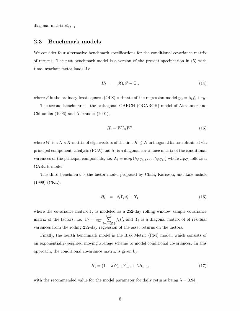
2.3 Benchmark models

We consider four alternative benchmark specifications for the conditional covariance matrix

of returns. The first benchmark model is a version of the present specification in (5) with

time-invariant factor loads, i.e.

Ht = βΩtβ′ + Ξt, (14)

where β is the ordinary least squares (OLS) estimate of the regression model yit = βift + εit.

The second benchmark is the orthogonal GARCH (OGARCH) model of Alexander and

Chibumba (1996) and Alexander (2001),

Ht =WΛtW′, (15)

whereW is a N×K matrix of eigenvectors of the first K ≤ N orthogonal factors obtained via

principal components analysis (PCA) and Λt is a diagonal covariance matrix of the conditional

variances of the principal components, i.e. Λt = diag (hPC1t , . . . , hPCkt) where hPCt follows a

GARCH model.

The third benchmark is the factor model proposed by Chan, Karceski, and Lakonishok

(1999) (CKL),

Ht = βtΓtβ′t +Υt, (16)

where the covariance matrix Γt is modeled as a 252-day rolling window sample covariance

matrix of the factors, i.e. Γt = 1252

t−1∑i=t−252

fif′i , and Υt is a diagonal matrix of of residual

variances from the rolling 252-day regression of the asset returns on the factors.

Finally, the fourth benchmark model is the Risk Metric (RM) model, which consists of

an exponentially-weighted moving average scheme to model conditional covariances. In this

approach, the conditional covariance matrix is given by

Ht = (1− λ)Yt−1Y′t−1 + λHt−1, (17)

with the recommended value for the model parameter for daily returns being λ = 0.94.

8

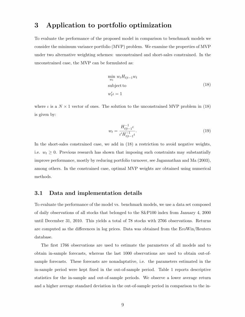
3 Application to portfolio optimization

To evaluate the performance of the proposed model in comparison to benchmark models we

consider the minimum variance portfolio (MVP) problem. We examine the properties of MVP

under two alternative weighting schemes: unconstrained and short-sales constrained. In the

unconstrained case, the MVP can be formulated as:

minwt

wtHt|t−1wt

subject to

w′tι = 1

(18)

where ι is a N × 1 vector of ones. The solution to the unconstrained MVP problem in (18)

is given by:

wt =H−1

t|t−1ι

ι′H−1t|t−1ι

. (19)

In the short-sales constrained case, we add in (18) a restriction to avoid negative weights,

i.e. wt ≥ 0. Previous research has shown that imposing such constraints may substantially

improve performance, mostly by reducing portfolio turnover, see Jagannathan and Ma (2003),

among others. In the constrained case, optimal MVP weights are obtained using numerical

methods.

3.1 Data and implementation details

To evaluate the performance of the model vs. benchmark models, we use a data set composed

of daily observations of all stocks that belonged to the S&P100 index from January 4, 2000

until December 31, 2010. This yields a total of 78 stocks with 2766 observations. Returns

are computed as the differences in log prices. Data was obtained from the EcoWin/Reuters

database.

The first 1766 observations are used to estimate the parameters of all models and to

obtain in-sample forecasts, whereas the last 1000 observations are used to obtain out-of-

sample forecasts. These forecasts are nonadaptative, i.e. the parameters estimated in the

in-sample period were kept fixed in the out-of-sample period. Table 1 reports descriptive

statistics for the in-sample and out-of-sample periods. We observe a lower average return

and a higher average standard deviation in the out-of-sample period in comparison to the in-

9

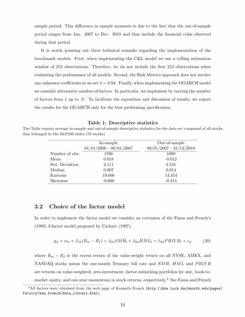
sample period. This difference in sample moments is due to the fact that the out-of-sample

period ranges from Jan. 2007 to Dec. 2010 and thus include the financial crisis observed

during that period.

It is worth pointing out three technical remarks regarding the implementation of the

benchmark models. First, when implementing the CKL model we use a rolling estimation

window of 252 observations. Therefore, we do not include the first 252 observations when

evaluating the performance of all models. Second, the Risk Metrics approach does not involve

any unknown coefficients as we set λ = 0.94. Finally, when implementing the OGARCHmodel

we consider alternative number of factors. In particular, we implement by varying the number

of factors from 1 up to N . To facilitate the exposition and discussion of results, we report

the results for the OGARCH only for the best performing specification.

Table 1: Descriptive statisticsThe Table reports average in-sample and out-of-sample descriptive statistics for the data set composed of all stocks

that belonged to the S&P100 index (78 stocks).

In-sample Out-of-sample01/01/2000 - 09/01/2007 09/01/2007 - 31/12/2010

Number of obs. 1766 1000Mean 0.018 -0.012Std. Deviation 2.111 2.541Median 0.007 0.014Kurtosis 19.666 14.454Skewness -0.600 -0.214

3.2 Choice of the factor model

In order to implement the factor model we consider an extension of the Fama and French’s

(1993) 3-factor model proposed by Carhart (1997),

yit = αit + β1it(Rm −Rf ) + β2itSMBt + β3itHMLt + β4itPR1Y Rt + εit (20)

where Rm − Rf is the excess return of the value-weight return on all NYSE, AMEX, and

NASDAQ stocks minus the one-month Treasury bill rate and SMB, HML and PR1Y R

are returns on value-weighted, zero-investment, factor-mimicking portfolios for size, book-to-

market equity, and one-year momentum in stock returns, respectively.4 See Fama and French

4All factors were obtained from the web page of Kenneth French (http://mba.tuck.dartmouth.edu/pages/faculty/ken.french/data_library.html).

10

(1993) and Carhart (1997) for details regarding the construction of these factor-mimicking

portfolios. Each parameter in (20) is time-varying and evolves according to (2) and (3).5

3.3 Methodology for evaluating performance

We examine the portfolios’ performance in terms of the variance of returns (σ2), Sharpe ratio

(SR) and turnover. These statistics are computed as follows:

σ2 =1

T − 1

T−1∑t=1

(w′tRt+1 − µ)2

SR =µ

σ, where µ =

1

T − 1

T−1∑t=1

w′tRt+1

Turnover =1

T − 1

T−1∑t=1

N∑j=1

(∣∣wj,t+1 − wj,t+∣∣),

where wj,t+ is the portfolio weight in asset j at time t+ 1 but before rebalancing and wj,t+1

is the desired portfolio weight in asset j at time t + 1. As pointed out by DeMiguel et al.

(2009), turnover as defined above can be interpreted as the average fraction of wealth traded

in each period.

To test the statistical significance of the difference between the variances and Sharpe

ratios of the returns for two given portfolios, we follow DeMiguel et al. (2009) and use

the stationary bootstrap of Politis and Romano (1994) with B=1,000 bootstrap resamples

and expected block length b=5.6 The resulting bootstrap p-values are obtained using the

methodology suggested in Ledoit and Wolf (2008, Remark 3.2).

3.4 Results

Table 2 reports the in-sample and out-of-sample portfolio variance, the Sharpe ratio and

the portfolio turnover of the short-sales constrained and unconstrained minimum variance

portfolio policies obtained with covariance matrices generated by the proposed model with

time-varying factor loads based on the RW model (FlexFGARCH-RW) and on the learning

model (FlexFGARCH-learning), and by the benchmark models. The benchmark models are

5In unreported results, we consider a version of the factor model in (20) with time-invariant alphas. The resultsare very similar to those reported here and are available upon request.

6We performed extensive robustness checks regarding the choice of the block length, using a range of values forb between 5 and 250. Regardless of the block length, the test results for the variances and Sharpe ratios are similarto those reported here.

11

the proposed model with time invariant factor loads (FlexFGARCH-OLS), the OGARCH

model, the Risk Metrics model, and the CKL model. The table also reports bootstrap p-

values for the differences between portfolios variance and Sharpe ratio with respect to those

obtained with the CKL model.

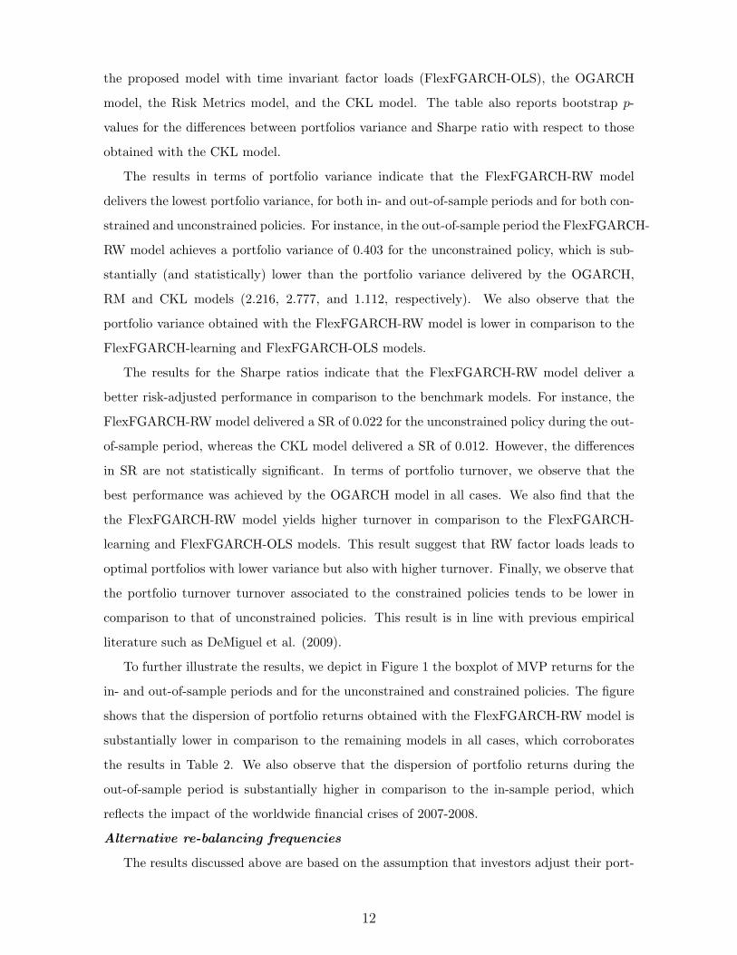
The results in terms of portfolio variance indicate that the FlexFGARCH-RW model

delivers the lowest portfolio variance, for both in- and out-of-sample periods and for both con-

strained and unconstrained policies. For instance, in the out-of-sample period the FlexFGARCH-

RW model achieves a portfolio variance of 0.403 for the unconstrained policy, which is sub-

stantially (and statistically) lower than the portfolio variance delivered by the OGARCH,

RM and CKL models (2.216, 2.777, and 1.112, respectively). We also observe that the

portfolio variance obtained with the FlexFGARCH-RW model is lower in comparison to the

FlexFGARCH-learning and FlexFGARCH-OLS models.

The results for the Sharpe ratios indicate that the FlexFGARCH-RW model deliver a

better risk-adjusted performance in comparison to the benchmark models. For instance, the

FlexFGARCH-RW model delivered a SR of 0.022 for the unconstrained policy during the out-

of-sample period, whereas the CKL model delivered a SR of 0.012. However, the differences

in SR are not statistically significant. In terms of portfolio turnover, we observe that the

best performance was achieved by the OGARCH model in all cases. We also find that the

the FlexFGARCH-RW model yields higher turnover in comparison to the FlexFGARCH-

learning and FlexFGARCH-OLS models. This result suggest that RW factor loads leads to

optimal portfolios with lower variance but also with higher turnover. Finally, we observe that

the portfolio turnover turnover associated to the constrained policies tends to be lower in

comparison to that of unconstrained policies. This result is in line with previous empirical

literature such as DeMiguel et al. (2009).

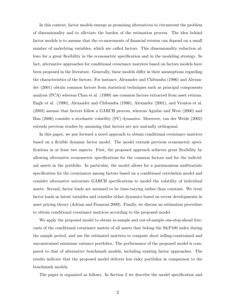
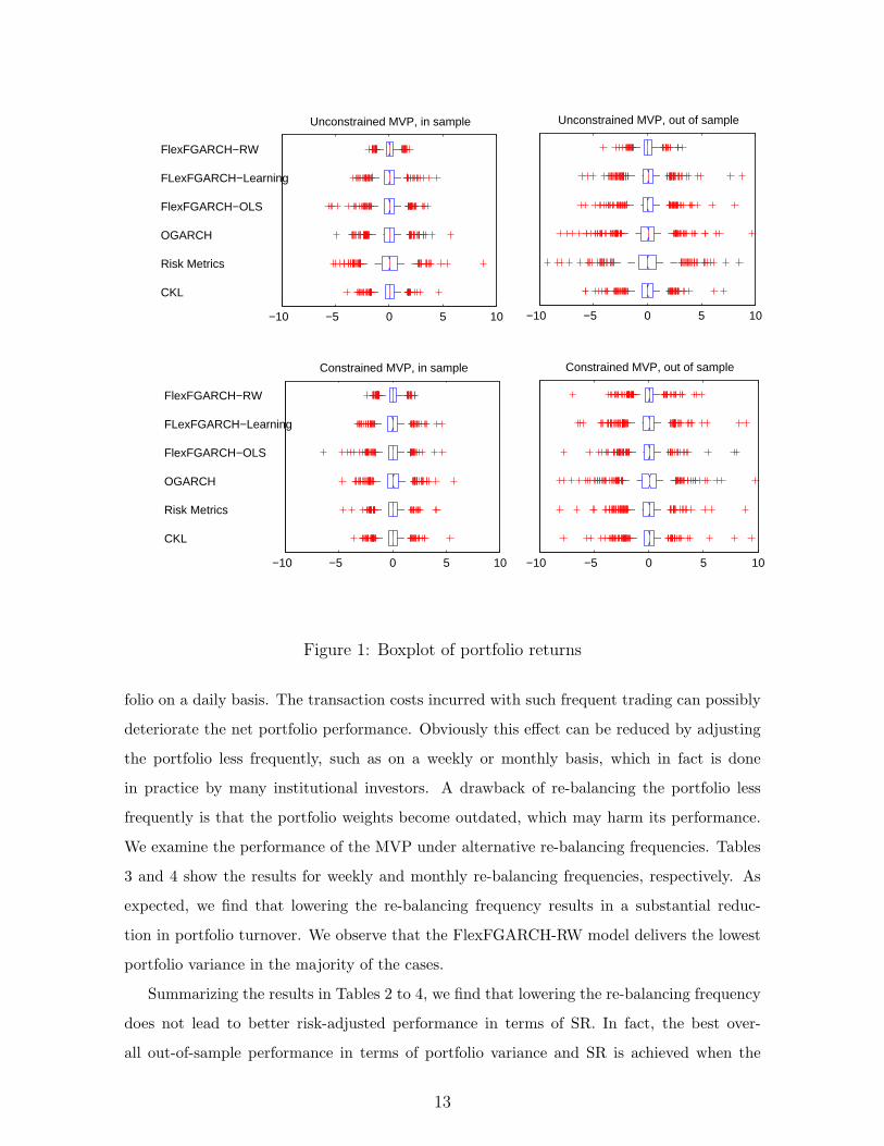
To further illustrate the results, we depict in Figure 1 the boxplot of MVP returns for the

in- and out-of-sample periods and for the unconstrained and constrained policies. The figure

shows that the dispersion of portfolio returns obtained with the FlexFGARCH-RW model is

substantially lower in comparison to the remaining models in all cases, which corroborates

the results in Table 2. We also observe that the dispersion of portfolio returns during the

out-of-sample period is substantially higher in comparison to the in-sample period, which

reflects the impact of the worldwide financial crises of 2007-2008.

Alternative re-balancing frequencies

The results discussed above are based on the assumption that investors adjust their port-

12

−10 −5 0 5 10

CKL

Risk Metrics

OGARCH

FlexFGARCH−OLS

FLexFGARCH−Learning

FlexFGARCH−RW

Unconstrained MVP, in sample

−10 −5 0 5 10

Unconstrained MVP, out of sample

−10 −5 0 5 10

CKL

Risk Metrics

OGARCH

FlexFGARCH−OLS

FLexFGARCH−Learning

FlexFGARCH−RW

Constrained MVP, in sample

−10 −5 0 5 10

Constrained MVP, out of sample

Figure 1: Boxplot of portfolio returns

folio on a daily basis. The transaction costs incurred with such frequent trading can possibly

deteriorate the net portfolio performance. Obviously this effect can be reduced by adjusting

the portfolio less frequently, such as on a weekly or monthly basis, which in fact is done

in practice by many institutional investors. A drawback of re-balancing the portfolio less

frequently is that the portfolio weights become outdated, which may harm its performance.

We examine the performance of the MVP under alternative re-balancing frequencies. Tables

3 and 4 show the results for weekly and monthly re-balancing frequencies, respectively. As

expected, we find that lowering the re-balancing frequency results in a substantial reduc-

tion in portfolio turnover. We observe that the FlexFGARCH-RW model delivers the lowest

portfolio variance in the majority of the cases.

Summarizing the results in Tables 2 to 4, we find that lowering the re-balancing frequency

does not lead to better risk-adjusted performance in terms of SR. In fact, the best over-

all out-of-sample performance in terms of portfolio variance and SR is achieved when the

13

FlexFGARCH-RW model is used to obtained unconstrained MVP under daily re-balancing.

4 Concluding remarks

Factor models are currently established as an alternative to alleviate the problem of dimen-

sionality and the burden of the estimation process when modeling covariance matrices of

portfolios containing a large number of assets. In this paper, we put forward a novel, flexible

approach to obtain conditional covariance matrices based on a factor model that extends pre-

vious econometric specifications. The proposed approach achieves great flexibility by allowing

a parsimonious specification for the common factors and alternative specifications the indi-

vidual assets in the portfolio. Moreover, we treat factor loads as time-varying latent variables

and consider richer dynamics based on recent developments in asset pricing theory.

We apply the proposed model to obtain in-sample and out-of-sample one-step-ahead fore-

casts of the conditional covariance matrix of all assets that belong the S&P100 index during

the sample period, and use the estimated matrices to compute short selling-constrained and

unconstrained minimum variance portfolios. The performance of the proposed model is com-

pared to that of alternative benchmark models, including existing factor approaches. The

results indicate that the proposed model delivers less risky portfolios in comparison to the

benchmark models.

14

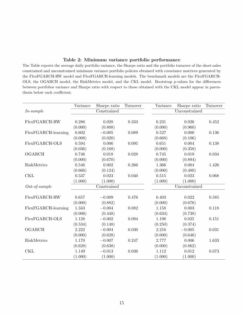
Table 2: Minimum variance portfolio performanceThe Table reports the average daily portfolio variance, the Sharpe ratio and the portfolio turnover of the short-sales

constrained and unconstrained minimum variance portfolio policies obtained with covariance matrices generated by

the FlexFGARCH-RW model and FlexFGARCH-learning models. The benchmark models are the FlexFGARCH-

OLS, the OGARCH model, the RiskMetrics model, and the CKL model. Bootstrap p-values for the differences

between portfolios variance and Sharpe ratio with respect to those obtained with the CKL model appear in paren-

thesis below each coefficient.

Variance Sharpe ratio Turnover Variance Sharpe ratio TurnoverIn-sample Constrained Unconstrained

FlexFGARCH-RW 0.286 0.028 0.333 0.231 0.026 0.452(0.000) (0.808) (0.000) (0.960)

FlexFGARCH-learning 0.602 −0.005 0.089 0.527 0.000 0.136(0.008) (0.020) (0.668) (0.106)

FlexFGARCH-OLS 0.594 0.006 0.095 0.651 0.004 0.138(0.036) (0.168) (0.000) (0.358)

OGARCH 0.746 0.018 0.028 0.745 0.019 0.034(0.000) (0.670) (0.000) (0.894)

RiskMetrics 0.546 0.002 0.266 1.366 0.004 1.426(0.666) (0.124) (0.000) (0.480)

CKL 0.537 0.023 0.040 0.515 0.023 0.068(1.000) (1.000) (1.000) (1.000)

Out-of-sample Constrained Unconstrained

FlexFGARCH-RW 0.657 −0.009 0.476 0.403 0.022 0.585(0.000) (0.882) (0.000) (0.676)


FlexFGARCH-OLS 1.128 −0.002 0.094 1.198 0.025 0.151(0.534) (0.148) (0.250) (0.374)

OGARCH 2.222 −0.004 0.030 2.216 −0.005 0.031(0.000) (0.628) (0.000) (0.646)

RiskMetrics 1.170 −0.007 0.247 2.777 0.006 1.633(0.628) (0.638) (0.000) (0.862)

CKL 1.149 −0.013 0.036 1.112 0.012 0.073(1.000) (1.000) (1.000) (1.000)

15

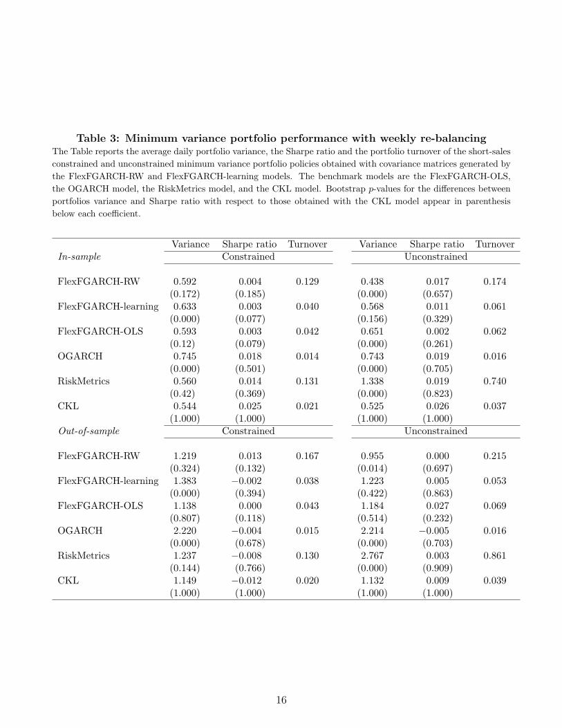
Table 3: Minimum variance portfolio performance with weekly re-balancingThe Table reports the average daily portfolio variance, the Sharpe ratio and the portfolio turnover of the short-sales


the FlexFGARCH-RW and FlexFGARCH-learning models. The benchmark models are the FlexFGARCH-OLS,

the OGARCH model, the RiskMetrics model, and the CKL model. Bootstrap p-values for the differences between

portfolios variance and Sharpe ratio with respect to those obtained with the CKL model appear in parenthesis

below each coefficient.


FlexFGARCH-RW 0.592 0.004 0.129 0.438 0.017 0.174(0.172) (0.185) (0.000) (0.657)

FlexFGARCH-learning 0.633 0.003 0.040 0.568 0.011 0.061(0.000) (0.077) (0.156) (0.329)

FlexFGARCH-OLS 0.593 0.003 0.042 0.651 0.002 0.062(0.12) (0.079) (0.000) (0.261)

OGARCH 0.745 0.018 0.014 0.743 0.019 0.016(0.000) (0.501) (0.000) (0.705)

RiskMetrics 0.560 0.014 0.131 1.338 0.019 0.740(0.42) (0.369) (0.000) (0.823)

CKL 0.544 0.025 0.021 0.525 0.026 0.037(1.000) (1.000) (1.000) (1.000)


FlexFGARCH-RW 1.219 0.013 0.167 0.955 0.000 0.215(0.324) (0.132) (0.014) (0.697)


FlexFGARCH-OLS 1.138 0.000 0.043 1.184 0.027 0.069(0.807) (0.118) (0.514) (0.232)

OGARCH 2.220 −0.004 0.015 2.214 −0.005 0.016(0.000) (0.678) (0.000) (0.703)

RiskMetrics 1.237 −0.008 0.130 2.767 0.003 0.861(0.144) (0.766) (0.000) (0.909)

CKL 1.149 −0.012 0.020 1.132 0.009 0.039(1.000) (1.000) (1.000) (1.000)

16

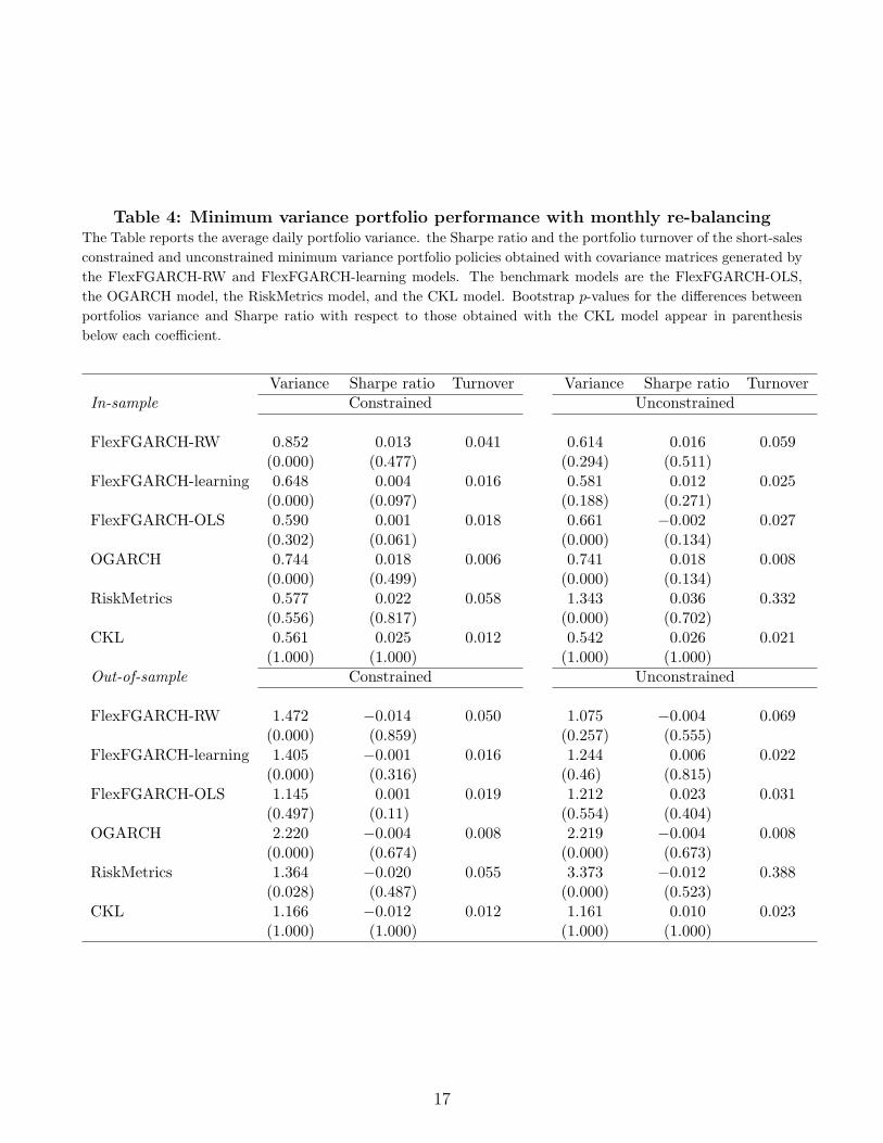
Table 4: Minimum variance portfolio performance with monthly re-balancingThe Table reports the average daily portfolio variance. the Sharpe ratio and the portfolio turnover of the short-sales


the FlexFGARCH-RW and FlexFGARCH-learning models. The benchmark models are the FlexFGARCH-OLS,

the OGARCH model, the RiskMetrics model, and the CKL model. Bootstrap p-values for the differences between

portfolios variance and Sharpe ratio with respect to those obtained with the CKL model appear in parenthesis

below each coefficient.


FlexFGARCH-RW 0.852 0.013 0.041 0.614 0.016 0.059(0.000) (0.477) (0.294) (0.511)

FlexFGARCH-learning 0.648 0.004 0.016 0.581 0.012 0.025(0.000) (0.097) (0.188) (0.271)

FlexFGARCH-OLS 0.590 0.001 0.018 0.661 −0.002 0.027(0.302) (0.061) (0.000) (0.134)

OGARCH 0.744 0.018 0.006 0.741 0.018 0.008(0.000) (0.499) (0.000) (0.134)

RiskMetrics 0.577 0.022 0.058 1.343 0.036 0.332(0.556) (0.817) (0.000) (0.702)

CKL 0.561 0.025 0.012 0.542 0.026 0.021(1.000) (1.000) (1.000) (1.000)


FlexFGARCH-RW 1.472 −0.014 0.050 1.075 −0.004 0.069(0.000) (0.859) (0.257) (0.555)


FlexFGARCH-OLS 1.145 0.001 0.019 1.212 0.023 0.031(0.497) (0.11) (0.554) (0.404)

OGARCH 2.220 −0.004 0.008 2.219 −0.004 0.008(0.000) (0.674) (0.000) (0.673)

RiskMetrics 1.364 −0.020 0.055 3.373 −0.012 0.388(0.028) (0.487) (0.000) (0.523)

CKL 1.166 −0.012 0.012 1.161 0.010 0.023(1.000) (1.000) (1.000) (1.000)

17

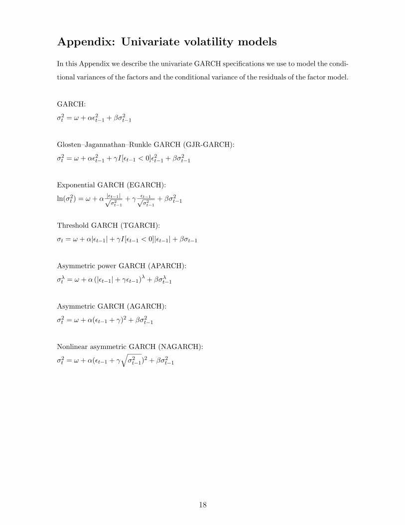
Appendix: Univariate volatility models

In this Appendix we describe the univariate GARCH specifications we use to model the condi-

tional variances of the factors and the conditional variance of the residuals of the factor model.

GARCH:

σ2t = ω + αϵ2t−1 + βσ2t−1

Glosten–Jagannathan–Runkle GARCH (GJR-GARCH):

σ2t = ω + αϵ2t−1 + γI[ϵt−1 < 0]ϵ2t−1 + βσ2t−1

Exponential GARCH (EGARCH):

ln(σ2t ) = ω + α |ϵt−1|√σ2t−1

+ γ ϵt−1√σ2t−1

+ βσ2t−1

Threshold GARCH (TGARCH):

σt = ω + α|ϵt−1|+ γI[ϵt−1 < 0]|ϵt−1|+ βσt−1

Asymmetric power GARCH (APARCH):

σλt = ω + α (|ϵt−1|+ γϵt−1)λ + βσλt−1

Asymmetric GARCH (AGARCH):

σ2t = ω + α(ϵt−1 + γ)2 + βσ2t−1

Nonlinear asymmetric GARCH (NAGARCH):

σ2t = ω + α(ϵt−1 + γ√σ2t−1)

2 + βσ2t−1

18

References

Adrian, T. and F. Franzoni (2009). Learning about beta: time-varying factor loadings,

expected returns, and the conditional capm. Journal of Empirical Finance 16 (4), 537–

556.

Aguilar, O. and M. West (2000). Bayesian dynamic factor models and portfolio allocation.

Journal of Business and Economic Statistics 18 (3), 338–357.

Alexander, C. (2001). Orthogonal GARCH. Mastering Risk 2, 21–38.

Alexander, C. and A. Chibumba (1996). Multivariate orthogonal factor GARCH. Working

paper, Mathematics Department, University of Sussex..

Ang, A. and J. Chen (2007). CAPM over the long run: 1926-2001. Journal of Empirical

Finance 14 (1), 1–40.

Bauwens, L., S. Laurent, and J. Rombouts (2006). Multivariate GARCH models: a survey.

Journal of Applied Econometrics 21 (1), 79–109.

Berkes, I., L. Horvath, and P. Kokoszka (2003). GARCH processes: structure and estima-

tion. Bernoulli 9 (2), 201–227.

Bollerslev, T. (1986). Generalized autoregressive conditional heteroskedasticity. Journal of

Econometrics 31 (3), 307–327.

Bollerslev, T., R. Engle, and J. Wooldridge (1988). A capital asset pricing model with

time-varying covariances. The Journal of Political Economy 96 (1), 116.

Bollerslev, T. and J. Wooldridge (1992). Quasi-maximum likelihood estimation and in-

ference in dynamic models with time-varying covariances. Econometric reviews 11 (2),

143–172.

Cappiello, L., R. Engle, and K. Sheppard (2006). Asymmetric dynamics in the correlations

of global equity and bond returns. Journal of Financial Econometrics 4 (4), 537–572.

Carhart, M. (1997). On persistence in mutual fund performance. The Journal of fi-

nance 52 (1), 57–82.

Chan, L., J. Karceski, and J. Lakonishok (1999). On portfolio optimization: forecasting

covariances and choosing the risk model. Review of Financial Studies 12 (5), 937–74.

Chib, S., Y. Omori, and M. Asai (2009). Multivariate stochastic volatility.

DeMiguel, V., L. Garlappi, F. Nogales, and R. Uppal (2009). A generalized approach to

portfolio optimization: improving performance by constraining portfolio norms. Man-

agement Science 55 (5), 798–812.

19

DeMiguel, V., L. Garlappi, and R. Uppal (2009). Optimal versus naive diversification: how

inefficient is the 1/N portfolio strategy? Review of Financial Studies 22 (5), 1915–1953.

Ding, Z., C. Granger, and R. Engle (1993). A long memory property of stock returns and

a new model. Journal of Empirical Finance 1 (1), 83–106.

Durbin, J. and S. J. Koopman (2001). Time series analysis by state space methods (2 ed.).

Oxford University Press.

Engle, R. (1990). Stock volatility and the crash of ’87: discussion. The Review of Financial

Studies 3 (1), 103–106.

Engle, R. (2002). Dynamic conditional correlation: a simple class of multivariate gen-

eralized autoregressive conditional heteroskedasticity models. Journal of Business &

Economic Statistics 20 (3), 339–350.

Engle, R. and K. Kroner (1995). Multivariate simultaneous generalized ARCH. Economet-

ric Theory 11 (1), 122–50.

Engle, R. and V. Ng (1993). Measuring and Testing the Impact of News on Volatility.

Journal of Finance 48 (5), 1749–78.

Engle, R., V. Ng, and M. Rothschild (1990). Asset pricing with a factor-arch covariance

structure: Empirical estimates for treasury bills. Journal of Econometrics 45 (1-2),

213–237.

Engle, R., N. Shephard, and K. Sheppard (2008). Fitting vast dimensional time-varying co-

variance models. Discussion Paper Series n.403, Department of Economics, University

of Oxford .

Engle, R. and K. Sheppard (2001). Theoretical and empirical properties of dynamic con-

ditional correlation multivariate GARCH. NBER Working Paper W8554 .

Fama, E. and K. French (1993). Common risk factors in the returns on stocks and bonds.

Journal of financial economics 33 (1), 3–56.

Francq, C. and J. Zakoian (2009). A tour in the asymptotic theory of GARCH estimation.

In T. Andersen, R. Davis, J.-P. Kreiss, and T. Mikosch (Eds.), Handbook of Financial

Time Series. Springer Verlag.

Glosten, L., R. Jagannathan, and D. Runkle (1993). On the relation between the expected

value and the volatility of the nominal excess return on stocks. Journal of Finance 48,

1779–1801.

Han, Y. (2006). Asset allocation with a high dimensional latent factor stochastic volatility

20

model. Review of Financial Studies 19 (1), 237–271.

Harvey, A., E. Ruiz, and N. Shephard (1994). Multivariate stochastic variance models.

Review of Economic Studies 61 (2), 247–64.

Jagannathan, R. and T. Ma (2003). Risk reduction in large portfolios: Why imposing the

wrong constraints helps. The Journal of Finance 58 (4), 1651–1684.

Jostova, G. and A. Philipov (2005). Bayesian analysis of stochastic betas. Journal of Fi-

nancial and Quantitative Analysis 40 (4), 747.

Koopman, S. J. (1997). Exact initial kalman filtering and smoothing for nonstationary time

series models. Journal of the American Statistical Association 92 (440), pp. 1630–1638.

Ledoit, O. and M. Wolf (2008). Robust performance hypothesis testing with the Sharpe

ratio. Journal of Empirical Finance 15 (5), 850–859.

Nelson, D. (1991). Conditional heteroskedasticity in asset returns: a new approach. Econo-

metrica 59 (2), 347–370.

Politis, D. and J. Romano (1994). The stationary bootstrap. Journal of the American

Statistical Association 89 (428), 1303–1313.

Robinson, P. and P. Zaffaroni (2006). Pseudo-maximum likelihood estimation of ARCH(∞)

models. The Annals of Statistics 34 (3), 1049–1074.

Sheppard, K. (2003). Multi-step estimation of multivariate GARCH models. In Proceedings

of the International ICSC. Symposium: Advanced Computing in Financial Markets.

Silvennoinen, A. and T. Terasvirta (2009). Multivariate GARCH models. In T. Andersen,

R. Davis, J.-P. Kreiss, and T. Mikosch (Eds.), Handbook of Financial Time Series.

Springer Verlag.

van der Weide, R. (2002). GO-GARCH: a multivariate generalized orthogonal GARCH

model. Journal of Applied Econometrics 17 (5), 549–564.

Vrontos, I., P. Dellaportas, and D. Politis (2003). A full-factor multivariate GARCH model.

The Econometrics Journal 6 (2), 312–334.

Zakoian, J. (1994). Threshold heteroskedastic models. Journal of Economic Dynamics and

control 18 (5), 931–955.

Zivot, E. (2009). Practical issues in the analysis of univariate GARCH models. In T. An-

dersen, R. Davis, J.-P. Kreiss, and T. Mikosch (Eds.), Handbook of Financial Time

Series. Springer Verlag.

21

Dynamic Factor Multivariate GARCH Model

Documents