doi: 10.1111/joes.12046 BAYESIAN INFERENCE METHODS FOR UNIVARIATE AND MULTIVARIATE GARCH MODELS: A SURVEY Audrone Virbickaite, M. Concepci´ on Aus´ ın and Pedro Galeano Departamento de Estad´ ıstica Universidad Carlos III de Madrid Abstract. This survey reviews the existing literature on the most relevant Bayesian inference methods for univariate and multivariate GARCH models. The advantages and drawbacks of each procedure are outlined as well as the advantages of the Bayesian approach versus classical procedures. The paper makes emphasis on recent Bayesian non-parametric approaches for GARCH models that avoid imposing arbitrary parametric distributional assumptions. These novel approaches implicitly assume infinite mixture of Gaussian distributions on the standardized returns which have been shown to be more flexible and describe better the uncertainty about future volatilities. Finally, the survey presents an illustration using real data to show the flexibility and usefulness of the non-parametric approach. Keywords. Bayesian inference; Dirichlet process mixture; Financial returns; GARCH models; Multivariate GARCH models; Volatility 1. Introduction Understanding, modelling and predicting the volatility of financial time series has been extensively researched for more than 30 years and the interest in the subject is far from decreasing. Volatility prediction has a very wide range of applications in finance, for example, in portfolio optimization, risk management, asset allocation, asset pricing. The two most popular approaches to model volatility are based on the Autoregressive Conditional Heteroscedasticity (ARCH)-type and Stochastic Volatility (SV)- type models. The seminal paper of Engle (1982) proposed the primary ARCH model while Bollerslev (1986) generalized the purely autoregressive ARCH into an ARMA-type model, called the Generalized Autoregressive Conditional Heteroscedasticity (GARCH) model. Since then, there has been a very large amount of research on the topic, stretching to various model extensions and generalizations. Meanwhile, the researchers have been addressing two important topics: looking for the best specification for the errors and selecting the most efficient approach for inference and prediction. Besides selecting the best model for the data, distributional assumptions for the returns are equally important. It is well known, that every prediction, in order to be useful, has to come with a certain precision measurement. In this way the agent can know the risk she is facing, that is, uncertainty. Distributional assumptions permit to quantify this uncertainty about the future. Traditionally, the errors have been assumed to be Gaussian, however, it has been widely acknowledged that financial returns display fat tails and are not conditionally Gaussian. Therefore, it is common to assume a Student-t distribution, see Bollerslev (1987), He and Ter¨ asvirta (1999) and Bai et al. (2003), among others. However, the assumption of Gaussian or Student-t distributions is rather restrictive. An alternative approach is to use a mixture Journal of Economic Surveys (2015) Vol. 29, No. 1, pp. 76–96 C 2013 John Wiley & Sons Ltd, 9600 Garsington Road, Oxford OX4 2DQ, UK and 350 Main Street, Malden, MA 02148, USA.

Welcome message from author
This document is posted to help you gain knowledge. Please leave a comment to let me know what you think about it! Share it to your friends and learn new things together.
Transcript
doi: 10.1111/joes.12046
BAYESIAN INFERENCE METHODS FORUNIVARIATE AND MULTIVARIATE GARCH
MODELS: A SURVEYAudrone Virbickaite, M. Concepcion Ausın and Pedro Galeano
Departamento de EstadısticaUniversidad Carlos III de Madrid
Abstract. This survey reviews the existing literature on the most relevant Bayesian inferencemethods for univariate and multivariate GARCH models. The advantages and drawbacks of eachprocedure are outlined as well as the advantages of the Bayesian approach versus classical procedures.The paper makes emphasis on recent Bayesian non-parametric approaches for GARCH models thatavoid imposing arbitrary parametric distributional assumptions. These novel approaches implicitlyassume infinite mixture of Gaussian distributions on the standardized returns which have been shownto be more flexible and describe better the uncertainty about future volatilities. Finally, the surveypresents an illustration using real data to show the flexibility and usefulness of the non-parametricapproach.
Keywords. Bayesian inference; Dirichlet process mixture; Financial returns; GARCH models;Multivariate GARCH models; Volatility
1. Introduction
Understanding, modelling and predicting the volatility of financial time series has been extensivelyresearched for more than 30 years and the interest in the subject is far from decreasing. Volatilityprediction has a very wide range of applications in finance, for example, in portfolio optimization, riskmanagement, asset allocation, asset pricing. The two most popular approaches to model volatility arebased on the Autoregressive Conditional Heteroscedasticity (ARCH)-type and Stochastic Volatility (SV)-type models. The seminal paper of Engle (1982) proposed the primary ARCH model while Bollerslev(1986) generalized the purely autoregressive ARCH into an ARMA-type model, called the GeneralizedAutoregressive Conditional Heteroscedasticity (GARCH) model. Since then, there has been a very largeamount of research on the topic, stretching to various model extensions and generalizations. Meanwhile,the researchers have been addressing two important topics: looking for the best specification for the errorsand selecting the most efficient approach for inference and prediction.
Besides selecting the best model for the data, distributional assumptions for the returns are equallyimportant. It is well known, that every prediction, in order to be useful, has to come with a certain precisionmeasurement. In this way the agent can know the risk she is facing, that is, uncertainty. Distributionalassumptions permit to quantify this uncertainty about the future. Traditionally, the errors have beenassumed to be Gaussian, however, it has been widely acknowledged that financial returns display fattails and are not conditionally Gaussian. Therefore, it is common to assume a Student-t distribution, seeBollerslev (1987), He and Terasvirta (1999) and Bai et al. (2003), among others. However, the assumptionof Gaussian or Student-t distributions is rather restrictive. An alternative approach is to use a mixture
Journal of Economic Surveys (2015) Vol. 29, No. 1, pp. 76–96C© 2013 John Wiley & Sons Ltd, 9600 Garsington Road, Oxford OX4 2DQ, UK and 350 Main Street, Malden,MA 02148, USA.
BAYESIAN INFERENCE METHODS FOR UNIVARIATE AND MULTIVARIATE GARCH MODELS 77
of distributions, which can approximate arbitrarily any distribution given a sufficient number of mixturecomponents. A mixture of two Normals was used by Bai et al. (2003), Ausın and Galeano (2007) andGiannikis et al. (2008), among others. These authors have shown that the models with the mixturedistribution for the errors outperformed the Gaussian one and do not require additional restrictions on thedegrees of freedom parameter as the Student-t one.
As for the inference and prediction, the Bayesian approach is especially well-suited for GARCHmodels and provides some advantages compared to classical estimation techniques, as outlined by Ardiaand Hoogerheide (2010). Firstly, the positivity constraints on the parameters to ensure positive variance,may encumber some optimization procedures. In the Bayesian setting, constraints on the model parameterscan be incorporated via priors. Secondly, in most of the cases we are more interested not in the modelparameters directly, but in some non-linear functions of them. In the maximum likelihood (ML) setting,it is quite troublesome to perform inference on such quantities, while in the Bayesian setting it isusually straightforward to obtain the posterior distribution of any non-linear function of the modelparameters. Furthermore, in the classical approach, models are usually compared by any other meansthan the likelihood. In the Bayesian setting, marginal likelihoods and Bayes factors allow for consistentcomparison of non-nested models while incorporating Occam’s razor for parsimony. Also, Bayesianestimation provides reliable results even for finite samples. Finally, Hall and Yao (2003) add that the MLapproach presents some limitations when the errors are heavy tailed, also the convergence rate is slowand the estimators may not be asymptotically Gaussian.
This survey reviews the existing Bayesian inference methods for univariate and multivariate GARCHmodels while having in mind their error specifications. The main emphasis of the paper is on the recentdevelopment of an alternative inference approach for these models using Bayesian non-parametrics. Theclassical parametric modelling, relying on a finite number of parameters, although so widely used, hassome certain drawbacks. Since the number of parameters for any model is fixed, one can encounterunderfitting or overfitting, which arises from the misfit between the data available and the parametersneeded to estimate. Then, in order to avoid assuming wrong parametric distributions, which may leadto inconsistent estimators, it is better to consider a semi- or non-parametric approach. Bayesian non-parametrics may lead to less constrained models than classical parametric Bayesian statistics and providean adequate description of the data, especially when the conditional return distribution is far away fromGaussian.
To our knowledge, there have been very few papers using Bayesian non-parametrics for GARCHmodels. These are Ausın et al. (2014) for univariate GARCH and Jensen and Maheu (2013) and Virbickaiteet al. (2013) for MGARCH. All of them have considered infinite mixtures of Gaussian distributions witha Dirichlet process (DP) prior over the mixing distribution, which results into DP mixture (DPM) models.This approach so far proves to be the most popular Bayesian non-parametric modelling procedure. Theresults over the papers have been consistent: The Bayesian non-parametric approach leads to more flexiblemodels and is better in explaining heavy-tailed return distributions, which parametric models cannot fullycapture.
The outline of this survey is as follows. Section 2 shortly introduces univariate GARCH models anddifferent inference and prediction methods. Section 3 overviews the existing models for multivariateGARCH and different inference and prediction approaches. Section 4 introduces the Bayesian non-parametric modelling approach and reviews the limited literature of this area in time-varying volatilitymodels. Section 5 presents a real data application. Finally, Section 6 concludes.
2. Univariate GARCH
As mentioned earlier, the two most popular approaches to model volatility are GARCH-type and SV-typemodels. In this survey we focus on GARCH models, therefore, SV models will not be included thereafter.
Journal of Economic Surveys (2015) Vol. 29, No. 1, pp. 76–96C© 2013 John Wiley & Sons Ltd
78 VIRBICKAITE ET AL.
Also, we are not going to enter into the technical details of the Bayesian algorithms and refer to Robertand Casella (2004) for a more detailed description of Bayesian techniques.
2.1 Description of Models
The general structure of an asset return series modelled by a GARCH-type model can be written as:
rt = μt + at = μt +√
htεt
where μt = E [rt |It−1] is the conditional mean given It−1, the information up to time t − 1, at is themean corrected returns of the asset at time t , ht = Var [rt |It−1] is the conditional variance given It−1
and εt is the standard white noise shock. There are several ways to model the conditional mean, μt .The usual assumptions are to consider that the mean is either zero, equal to a constant (μt = μ), orfollows an ARMA(p,q) process. However, sometimes the mean is also modelled as a function of thevariance, say g(ht ), which leads to the GARCH-in-Mean models. On the other hand, the conditionalvariance, ht , is usually modelled using the GARCH-family models. In the basic GARCH model, theconditional variance of the returns depends on a sum of three parts: a constant variance as the long-runaverage, a linear combination of the past conditional variances and a linear combination of the past meansquared returns. For instance, in the GARCH(1,1) model, the conditional variance at time t is given byht = ω + αa2
t−1 + βht−1, for t = 1, . . . , T . There are some restrictions which have to be imposed suchas ω > 0, α, β ≥ 0 for positive variance, and α + β < 1 for the covariance stationarity.
Nelson (1991) proposed the exponential GARCH (EGARCH) model that acknowledges the existenceof asymmetry in the volatility response to the changes in the returns, sometimes also called the ‘leverageeffect’, introduced by Black (1976). Negative shocks to the returns have a stronger effect on volatility thanpositive. Other ARCH extensions that try to incorporate the leverage effect are the Glosten–Jagannathan–Runkle (GJR) model by Glosten et al. (1993) and the TGARCH of Zakoian (1994), among many others.As Engle (2004) puts it, ‘there is now an alphabet soup’ of ARCH family models, such as AARCH,APARCH, FIGARCH, STARCH, which try to incorporate such return features as fat tails, volatilityclustering and volatility asymmetry. Papers by Bollerslev et al. (1992), Bollerslev et al. (1994), Engle(2002b) and Ishida and Engle (2002) provide extensive reviews of the existing ARCH-type models. Beraand Higgins (1993) review ARCH-type models, discuss their extensions, estimation and testing alsonumerous applications. Also, one can find an explicit review with examples and applications concerningGARCH-family models in Tsay (2010) and chapter 1 in Terasvirta (2009).
2.2 Inference Methods
The main estimation approach for GARCH-family models is the classical ML method. However, recentlythere has been a rapid development of Bayesian estimation techniques, which offer some advantagescompared to the frequentist approach as already discussed in the Introduction. In addition, in the empiricalfinance setting, the frequentist approach presents an uncertainty problem. For instance, optimal allocationis greatly affected by the parameter uncertainty, which has been recognized in a number of papers, seeJorion (1986) and Greyserman et al. (2006), among others. These authors conclude that in the frequentistsetting the estimated parameter values are considered to be the true ones, therefore, the optimal portfolioweights tend to inherit this estimation error. However, instead of solving the optimization problem onthe basis of the choice of unique parameter values, the investor can choose the Bayesian approach,because it accounts for parameter uncertainty, as seen in Kang (2011) and Jacquier and Polson (2013), forexample. A number of papers in this field have explored different Bayesian procedures for inference andprediction and different approaches to modelling the fat-tailed errors and/or asymmetric volatility. Therecent development of modern Bayesian computational methods, based on Monte Carlo approximations
Journal of Economic Surveys (2015) Vol. 29, No. 1, pp. 76–96C© 2013 John Wiley & Sons Ltd
BAYESIAN INFERENCE METHODS FOR UNIVARIATE AND MULTIVARIATE GARCH MODELS 79
and Markov Chain Monte Carlo (MCMC) methods have facilitated the usage of Bayesian techniques, seefor example, Robert and Casella (2004).
The standard Gibbs sampling procedure does not make the list because it cannot be used due to therecursive nature of the conditional variance: the conditional posterior distributions of the model parametersare not of a simple form. One of the alternatives is the Griddy–Gibbs sampler as in Bauwens and Lubrano(1998). They discuss that previously used importance sampling and Metropolis algorithms have certaindrawbacks, such as that they require a careful choice of a good approximation of the posterior density.The authors propose a Griddy–Gibbs sampler which explores analytical properties of the posterior densityas much as possible. In this paper the GARCH model has Student-t errors, which allows for fat tails.The authors choose to use flat (uniform) priors on parameters (ω, α, β) with whatever region is neededto ensure the positivity of variance, however, the flat prior for the degrees of freedom cannot be used,because then the posterior density is not integrable. Instead, they choose a half-right side of Cauchy. Theposteriors of the parameters were found to be skewed, which is a disadvantage for the commonly usedGaussian approximation. On the other hand, Ausın and Galeano (2007) modelled the errors of a GARCHmodel with a mixture of two Gaussian distributions. The advantage of this approach compared to that ofStudent-t errors, is that if the number of the degrees of freedom is very small (less than 5), some momentsmay not exist. The authors have chosen flat priors for all the parameters, and discovered that there is littlesensitivity to the change in the prior distributions (from uniform to Beta), unlike in Bauwens and Lubrano(1998), where the sensitivity for the prior choice for the degrees of freedom is high. More articles using aGriddy–Gibbs sampling approach are by Bauwens and Lubrano (2002), who have modelled asymmetricvolatility with Gaussian innovations and have used uniform priors for all the parameters, and by Wago(2004), who explored an asymmetric GARCH model with Student-t errors.
Another MCMC algorithm used in estimating GARCH model parameters, is the Metropolis–Hastings(MH) method, which samples from a candidate density and then accepts or rejects the draws dependingon a certain acceptance probability. Ardia (2006) modelled the errors as Gaussian distributed with zeromean and unit variance while the priors are chosen as Gaussian, and an MH algorithm is used todraw samples from the joint posterior distribution. The author has carried out a comparative analysisbetween ML and Bayesian approaches, finding, as in other papers, that some posterior distributions ofthe parameters were skewed, thus warning against the abusive use of the Gaussian approximation. Also,Ardia (2006) has performed a sensitivity analysis of the prior means and scale parameters and concludedthat the initial priors in this case are vague enough. This approach has been also used by Muller and Pole(1998), Nakatsuma (2000) and Vrontos et al. (2000), among others. A special case of the MH methodis the random walk Metropolis–Hastings (RWMH) where the proposal draws are generated by randomlyperturbing the current value using a spherically symmetric distribution. A usual choice is to generatecandidate values from a Gaussian distribution where the mean is the previous value of the parameter andthe variance can be calibrated to achieve the desired acceptance probability. This procedure is repeatedat each MCMC iteration. Ausın and Galeano (2007) have also carried out a comparison of estimationapproaches, Griddy–Gibbs, RWMH and ML. Apparently, RWMH has difficulties in exploring the tails ofthe posterior distributions and ML estimates may be rather different for those parameters where posteriordistributions are skewed.
In order to select one of the algorithms, one might consider some criteria, such as fast convergence forexample. Asai (2006) numerically compares some of these approaches in the context of GARCH. TheGriddy–Gibbs method is capable in handling the shape of the posterior by using smaller MCMC outputscomparing with other methods, also, it is flexible regarding parametric specification of a model. However,it can require a lot of computational time. This author also investigates MH, adaptive rejection Metropolissampling (ARMS), proposed by Gilks et al. (1995), and acceptance–rejection MH algorithms (ARMH),proposed by Tierney (1994). For more detail about each method in GARCH models see Nakatsuma(2000) and Kim et al. (1998), among others. Using simulated data, Asai (2006) calculated geometricaverages of inefficiency factors for each method. Inefficiency factor is just an inverse of Geweke (1992)
Journal of Economic Surveys (2015) Vol. 29, No. 1, pp. 76–96C© 2013 John Wiley & Sons Ltd
80 VIRBICKAITE ET AL.
efficiency factor. According to this, the ARMH algorithm performed the best. Also, computational timewas taken into consideration, where ARMH clearly outperformed MH and ARMS, while Griddy–Gibbsstayed just a bit behind. The author observes that even though the ARMH method showed the best results,the posterior densities for each parameter did not quite explore the tails of the distributions, as desired. Inthis case Griddy–Gibbs performs better; also, it requires less draws than ARMH. Bauwens and Lubrano(1998) investigate one more convergence criteria, proposed by Yu and Mykland (1998), which is based oncumulative sum (cumsum) statistics. It basically shows that if MCMC is converging, the graph of a certaincumsum statistic against time should approach zero. Their employed Griddy–Gibbs algorithm convergedin all four parameters quite fast. Then, the authors explored the advantages and disadvantages of alternativeapproaches: the importance sampling and the MH algorithm. Considering importance sampling, one ofthe main disadvantages, as mentioned before, is to find a good approximation of the posterior density(importance function). Also, comparing with Griddy–Gibbs algorithm, the importance sampling requiresmuch more draws to get smooth graphs of the marginal densities. For the MH algorithm, same as inimportance sampling, a good approximation needs to be found. Also, compared to Griddy–Gibbs, theMH algorithm did not fully explore the tails of the distribution, unless for a very big number of draws.
Another important aspect of the Bayesian approach, as commented before, are the advantages in modelselection compared to the classical methods. Miazhynskaia and Dorffner (2006) review some Bayesianmodel selection methods using MCMC for GARCH-type models, which allow for the estimation of eithermarginal model likelihoods, Bayes factors or posterior model probabilities. These are compared to theclassical model selection criteria showing that the Bayesian approach clearly considers model complexityin a more unbiased way. Also, Chen et al. (2009) includes a revision of Bayesian selection methods forasymmetric GARCH models, such as the GJR–GARCH and threshold GARCH. They show how usingthe Bayesian approach it is possible to compare complex and non-nested models to choose, for example,between GARCH and SV models, between symmetric or asymmetric GARCH models or to determinethe number of regimes in threshold processes, among others.
An alternative approach to the previous parametric specifications is the use of Bayesian non-parametricmethods, that allow to model the errors as an infinite mixture of normals, as seen in the paper by Ausınet al. (2014). The Bayesian non-parametric approach for time-varying volatility models will be discussedin detail in Section 4.
To sum up, considering the amount of articles published quite recently regarding the topic of estimatingunivariate GARCH models using MCMC methods indicates still growing interest in the area. Althoughnumerous GARCH-family models have been investigated using different MCMC algorithms, there arestill a lot of areas that need further research and development.
3. Multivariate GARCH
Returns and volatilities depend on each other, so multivariate analysis is a more natural and usefulapproach. The starting point of multivariate volatility models is a univariate GARCH, thus the most simpleMGARCH models can be viewed as direct generalizations of their univariate counterparts. Consider amultivariate return series {rt }T
t=1 of size K × 1. Then
rt = μt + at = μt + H 1/2t εt
where μt = E[rt |It−1], at are mean-corrected returns, εt is a random vector, such that E[εt ] = 0 andCov[εt ] = IK and H 1/2
t is a positive definite matrix of dimensions K × K , such that Ht is the conditionalcovariance matrix of rt , that is, Cov[rt |It−1] = H 1/2
t Cov[εt ](H 1/2t )′ = Ht . There is a wide range of
MGARCH models, where most of them differ in specifying Ht . In the rest of this section we will reviewthe most popular and widely used, and the different Bayesian approaches to make inference and prediction.
Journal of Economic Surveys (2015) Vol. 29, No. 1, pp. 76–96C© 2013 John Wiley & Sons Ltd
BAYESIAN INFERENCE METHODS FOR UNIVARIATE AND MULTIVARIATE GARCH MODELS 81
For general reviews on MGARCH models, see Bauwens et al. (2006), Silvennoinen and Terasvirta (2009)and (Tsay, 2010, chapter 10), among others.
Regarding inference, one can also consider the same arguments provided in the univariate GARCH casementioned above. ML estimation for MGARCH models can be obtained by using numerical optimizationalgorithms, such as Fisher scoring and Newton–Raphson. Vrontos et al. (2003b) have estimated severalbivariate ARCH and GARCH models and found that some classical estimates of the parameters were quitedifferent from their Bayesian counterparts. This was due to the non-normality of the parameters. Thus, theauthors suggest careful interpretation of the classical estimation approach. Also, Vrontos et al. (2003b)found it difficult to evaluate the classical estimates under the stationarity conditions, and consequently theresulting parameters, evaluated ignoring the stationarity constraints, produced non-stationary estimates.These difficulties can be overcome using the Bayesian approach.
3.1 VEC, DVEC and BEKK
The VEC model was proposed by Bollerslev et al. (1988), where every conditional variance and covariance(elements of the Ht matrix) is a function of all lagged conditional variances and covariances, as wellas lagged squared mean-corrected returns and cross-products of returns. Using this unrestricted VECformulation, the number of parameters increases dramatically. For example, if K = 3, the number ofparameters to estimate will be 78, and if K = 4, the number of parameters increases to 210, see Bauwenset al. (2006) for the explicit formula for the number of parameters in VEC models. To overcome thisdifficulty, Bollerslev et al. (1988) simplified the VEC model by proposing a diagonal VEC model, ordiagonal VEC (DVEC), as follows:
Ht = � + A � (at−1a′t−1) + B � Ht−1
where � indicates the Hadamard product, �, A and B are symmetric K × K matrices. As noted inBauwens et al. (2006), Ht is positive definite provided that �, A, B and the initial matrix H0 are positivedefinite. However, these are quite strong restrictions on the parameters. Also, DVEC model does notallow for dynamic dependence between volatility series. In order to avoid such strong restrictions on theparameter matrices, Engle and Kroner (1995) propose the BEKK (Baba, Engle, Kraft and Kroner) model,which is just a special case of a VEC and, consequently, less general. It has the attractive property thatthe conditional covariance matrices are positive definite by construction. The model looks as follows:
Ht = �∗�∗′ + A∗(at−1a′t−1)A∗′ + B∗ Ht−1 B∗′
(1)
where �∗ is a lower triangular matrix and A∗ and B∗ are K × K matrices. In the BEKK model it is easyto impose the definite positiveness of the Ht matrix. However, the parameter matrices A∗ and B∗ do nothave direct interpretations since they do not represent directly the size of the impact of the lagged valuesof volatilities and squared returns.
Osiewalski and Pipien (2004) present a paper that compares the performance of various bivariateARCH and GARCH models, such as VEC, BEKK, estimated using Bayesian techniques. As the authorsobserve, they are the first to perform model comparison using Bayes factors and posterior odds in theMGARCH setting. The algorithm used for parameter estimation and inference is MH, and to checkfor convergence they rely on the cumsum statistics, introduced by Yu and Mykland (1998), and used byBauwens and Lubrano (1998) in the univariate GARCH setting. Using the real data, the authors found thatthe t-BEKK models performed the best, leaving t-VEC not so far behind; t-VEC model, sometimes alsocalled t-VECH, is a more general form of a DVEC, seen above, where the mean-corrected returns follow aStudent-t distribution. The name comes from a function called vech, which reshapes the lower triangularportion of a symmetric variance–covariance matrix into a column vector. To sum up, the authors choose
Journal of Economic Surveys (2015) Vol. 29, No. 1, pp. 76–96C© 2013 John Wiley & Sons Ltd
82 VIRBICKAITE ET AL.
t-BEKK model as clearly better than the t-VEC, because it is relatively simple and has less parameters toestimate.
On the other hand, Hudson and Gerlach (2008) developed a prior distribution for a VECH specificationthat directly satisfies both necessary and sufficient conditions for positive definiteness and covariancestationarity, while remaining diffuse and non-informative over the allowable parameter space. Theseauthors employed MCMC methods, including MH, to help enforce the conditions in this prior.
More recently, Burda and Maheu (2013) use the BEKK–GARCH model to show the usefulness of anew posterior sampler called the Adaptive Hamiltonian Monte Carlo (AHMC). Hamiltonian Monte Carlo(HMC) is a procedure to sample from complex distributions. The AHMC is an alternative inferentialmethod based on HMC that is both fast and locally adaptive. The AHMC appears to work very well whenthe dimension of the parameter space is very high. Model selection based on marginal likelihood is usedto show that full BEKK models are preferred to restricted diagonal specifications. Additionally, Burda(2013) suggests an approach called Constrained Hamiltonian Monte Carlo (CHMC) in order to deal withhigh-dimensional BEKK models with targeting, which allow for a parameter dimension reduction withoutcompromising the model fit, unlike the diagonal BEKK. Model comparison of the full BEKK and theBEKK with targeting is performed indicating that the latter dominates the former in terms of marginallikelihood.
3.2 Factor-GARCH
Factor-GARCH was first proposed by Engle et al. (1990) to reduce the dimension of the multivariatemodel of interest using an accurate approximation of the multivariate volatility. The definition of theFactor-GARCH model, proposed by Lin (1992), says that BEKK model in (1) is a Factor-GARCH, if A∗and B∗ have rank one and the same left and right eigenvalues: A∗ = αwλ′, B∗ = βwλ′, where α and β
are scalars and w and λ are eigenvectors. Several variants of the factor model have been proposed. Oneof them is the full-factor multivariate GARCH by Vrontos et al. (2003a):
rt = μ + at
at = W Xt
Xt |It−1 ∼ NK (0, �t )
where μ is a K × 1 vector of constants, which is time invariant, W is a K × K parameter matrix, Xt isa K × 1 vector of factors and �t = diag(σ 2
1t , . . . , σ2K t ) is a K × K diagonal variance matrix such that
σ 2i t = ci + bi x2
i,t−1 + giσ2i,t−1, where σ 2
i t is the conditional variance of the i th factor at time t such thatci > 0, bi ≥ 0, gi ≥ 0. Then, the factors in the Xt vector are GARCH(1,1) processes and the vector at is alinear combination of such factors. It can be easily shown that Ht is always positive definite by construction.However, the structure of Ht depends on the order of the time series in rt . Vrontos et al. (2003a) haveconsidered this problem to find the best ordering under the proposed model. Furthermore, Vrontos et al.(2003a) investigate a full-factor MGARCH model using the ML and Bayesian approaches. The authorscompute ML estimates using Fisher scoring algorithm. As for the Bayesian analysis, the authors haveadopted an MH algorithm, and found that the algorithm is very time consuming, especially in high-dimensional data. To speed-up the convergence, Vrontos et al. (2003a) have proposed reparametrizationof positive parameters and also a blocking sampling scheme, where the parameter vector is dividedinto three blocks: mean, variance and the matrix of constants W . As mentioned before, the ordering ofthe univariate time series in full-factor models is important, thus to select ‘the best’ model one has toconsider K ! possibilities for a multivariate data set of dimension K . Instead of choosing one model andmaking inference (as if the selected model was the true one), the authors employ a Bayesian approachby calculating the posterior probabilities for all competing models and model averaging to provide‘combined’ predictions. The main contribution of this paper is that the authors were able to carry out an
Journal of Economic Surveys (2015) Vol. 29, No. 1, pp. 76–96C© 2013 John Wiley & Sons Ltd
BAYESIAN INFERENCE METHODS FOR UNIVARIATE AND MULTIVARIATE GARCH MODELS 83
extensive Bayesian analysis of a full-factor MGARCH model considering not only parameter uncertainty,but model uncertainty as well.
As already discussed, a very common stylized feature of financial time series is the asymmetricvolatility. Dellaportas and Vrontos (2007) have proposed a new class of tree structured MGARCH modelsthat explore the asymmetric volatility effect. Same as the paper by Vrontos et al. (2003a), the authorsconsider not only parameter-related uncertainty, but also uncertainty corresponding to model selection.Thus in this case, Bayesian approach becomes particularly useful because an alternative method basedon maximizing the pseudo-likelihood is only able to work after selecting a single model. The authorsdevelop an MCMC stochastic search algorithm that generates candidate tree structures and their posteriorprobabilities. The proposed algorithm converged fast. Such modelling and inference approach leads tomore reliable and more informative results concerning model selection and individual parameter inference.
There are more models that are nested in BEKK, such as the Orthogonal GARCH for example,see Alexander and Chibumba (1997) and Van der Weide (2002), among others. All of them fall intothe class of direct generalizations of univariate GARCH or linear combinations of univariate GARCHmodels. Another class of models are the non-linear combinations of univariate GARCH models, such asconditional correlation (CCC), dynamic condition correlation (DCC), general dynamic covariance (GDC)and Copula–GARCH models. A very recent alternative approach that also considers Bayesian estimationcan be found in Jin and Maheu (2013) who proposes a new dynamic component models of returns andrealized covariance (RCOV) matrices based on time-varying Wishart distributions. In particular, Bayesianestimation and model comparison is conducted with an existing range of multivariate GARCH modelsand RCOV models.
3.3 CCC
The CCC model, proposed by Bollerslev (1990) and the simplest in its class, is based on the decompositionof the conditional covariance matrix into conditional standard deviations and correlations. Then, theconditional covariance matrix Ht looks as follows:
Ht = Dt RDt
where Dt is diagonal matrix with the K conditional standard deviations and R is a time-invariant CCCmatrix such that R = (ρi j ) and ρi j = 1,∀i = j . The CCC approach can be applied to a wide range ofunivariate GARCH family models, such as exponential GARCH or GJR–GARCH, for example.
Vrontos et al. (2003b) have estimated some real data using a variety of bivariate ARCH and GARCHmodels in order to select the best model specification and to compare the Bayesian parameter estimatesto those of the ML. These authors have considered three ARCH and three GARCH models, all of themwith constant CCCs. They have used an MH algorithm, which allows to simulate from the joint posteriordistribution of the parameters. For model comparison and selection, Vrontos et al. (2003b) have obtainedpredictive distributions and assessed comparative validity of the analysed models, according to which theCCC model with diagonal covariance matrix performed the best considering one-step-ahead predictions.
3.4 DCC
A natural extension of the simple CCC model are the DCC models, first proposed by Tse and Tsui (2002)and Engle (2002a). The DCC approach is more realistic, because the dependence between returns is likelyto be time varying.
The models proposed by Tse and Tsui (2002) and Engle (2002a) consider that the conditional covariancematrix Ht looks as Ht = Dt Rt Dt , where Rt is now a time-varying correlation matrix at time t . Themodels differ in the specification of Rt . In the paper by Tse and Tsui (2002), the CCC matrix is
Journal of Economic Surveys (2015) Vol. 29, No. 1, pp. 76–96C© 2013 John Wiley & Sons Ltd
84 VIRBICKAITE ET AL.
Rt = (1 − θ1 − θ2)R + θ1 Rt−1 + θ2�t−1, where θ1 and θ2 are non-negative scalar parameters, such thatθ1 + θ2 < 1, R is a positive definite matrix such that ρi i = 1 and �t−1 is a K × K sample correlationmatrix of the past m standardized mean-corrected returns ut = D−1
t at . On the other hand, in the paperby Engle (2002a), the specification of Rt is Rt = (I � Qt )−1/2 Qt (I � Qt )−1/2, where Qt = (1 − α −β)Q + α(ut−1u′
t−1) + βQt−1, ui,t = ai,t/√
hii,t is a mean-corrected standardized returns, α and β arenon-negative scalar parameters, such that α + β < 1 and Q is an unconditional covariance matrix of ut .As noted in Bauwens et al. (2006), the model by Engle (2002a) does not formulate the CCC as a weightedsum of past correlations, unlike in the DCC model by Tse and Tsui (2002), seen earlier. The drawbackof both these models is that θ1, θ2, α and β are scalar parameters, so all CCCs have the same dynamics.However, as Tsay (2010) notes it, the models are parsimonious.
Moreover, as financial returns display not only asymmetric volatility, but also excess kurtosis, previousresearch, as in univariate case, has mostly considered using a multivariate Student-t distribution for theerrors. However, as already discussed, this approach has several limitations. Galeano and Ausın (2010)propose an MGARCH–DCC model, where the standardized innovations follow a mixture of Gaussiandistributions. This allows to capture long tails without being limited by the degrees of freedom constraint,which is necessary to impose in the Student-t distribution so that higher moments could exist. The authorsestimate the proposed model using the classical ML and Bayesian approaches. In order to estimate modelparameters, dynamics of single assets and dynamic correlations, and the parameters of the Gaussianmixture, Galeano and Ausın (2010) have relied on RWMH algorithm. BIC criteria was used for selectingthe number of mixture components, which performed well in simulated data. Using real data, the authorsprovide an application to calculating the Value at Risk (VaR) and solving a portfolio selection problem.MLE and Bayesian approaches have performed similarly in point estimation, however, the Bayesianapproach, besides giving just point estimates, allows the derivation of predictive distributions for theportfolio VaR.
An extension of the DCC model of Engle (2002a) is the Asymmetric DCC also proposed by Engle(2002a), which incorporates an asymmetric correlation effect. It means that correlations between assetreturns decrease more in the bear market than they increase when the market performs well. Cappielloet al. (2006) generalizes the ADCC model into the AGDCC model, where the parameters of the correlationequation are vectors, and not scalars. This allows for asset-specific correlation dynamics. In the AGDCCmodel, the Qt matrix in the DCC model is replaced with:
Qt = S(1 − κ2 − λ2 − δ2/2) + κκ ′ � u′t−1ut−1 + λλ′ � Qt−1 + δδ′ � η′
t−1ηt−1
where ut = D−1t at are mean corrected standardized returns, ηt = ut � I (ut < 0) selects just negative
returns, ‘diag’ stands for either taking just the diagonal elements from the matrix, or making a diagonalmatrix from a vector, S is a sample correlation matrix of ut , κ, λ and δ are K × 1 vectors, κ = K −1 ∑K
i=1 κi ,λ = K −1 ∑K
i=1 λi and δ = K −1 ∑Ki=1 δi . To ensure positivity and stationarity of Qt , it is necessary to
impose κi , λi , δi > 0 and κ2i + λ2
i + δ2i /2 < 1, ∀i = 1, . . . , K . The AGDCC by Cappiello et al. (2006)
is just a special case where κ1 = . . . = κK , λ1 = . . . = λK and δ1 = . . . = δK .To our knowledge, the only paper that considers the AGDCC model in the Bayesian setting is Virbickaite
et al. (2013) that propose to model the distribution of the standardized returns as an infinite scale mixtureof Gaussian distributions by relying on Bayesian non-parametrics. This approach is presented in moredetail in Section 4.
3.5 Copula–GARCH
The use of copulas is an alternative approach to study return time series and their volatilities. The mainconvenience of using copulas is that individual marginal densities of the returns can be defined separatelyfrom their dependence structure. Then, each marginal time series can be modelled using univariate
Journal of Economic Surveys (2015) Vol. 29, No. 1, pp. 76–96C© 2013 John Wiley & Sons Ltd
BAYESIAN INFERENCE METHODS FOR UNIVARIATE AND MULTIVARIATE GARCH MODELS 85
specification and the dependence between the returns can be modelled by selecting an appropriatecopula function. A K -dimensional copula C(u1, . . . , uK ), is a multivariate distribution function in theunit hypercube [0, 1]K , with uniform [0, 1] marginal distributions. Under certain conditions, the SklarTheorem affirms that (see, Sklar, 1959), every joint distribution F(x1, . . . , xK ), whose marginals are givenby F1(x1), . . . , FK (xK ), can be written as F(x1, . . . , xK ) = C(F1(x1), . . . , FK (xK )), where C is a copulafunction of F , which is unique if the marginal distributions are continuous.
The most popular approach to volatility modelling through copulas is called the Copula–GARCHmodel, where univariate GARCH models are specified for each marginal series and the dependencestructure between them is described using a copula function. A very useful feature of copulas, as noted byPatton (2009), is that the marginal distributions of each random variable do not need to be similar to eachother. This is very important in modelling time series, because each of them might be following differentdistributions. The choice of copulas can vary from a simple Gaussian copula to more flexible ones, such asClayton, Gumbel and mixed Gaussian. In the existing literature, different parametric and non-parametricspecifications can be used for the marginals and copula function C . Also, the copula function can beassumed to be constant or time varying, as seen in Ausın and Lopes (2010), among others.
The estimation for Copula–GARCH models can be performed in a variety of ways. ML is the obviouschoice for fully parametric models. Estimation is generally based on a multistage method, where firstly theparameters of the marginal univariate distributions are estimated and then used to condition in estimatingthe parameters of the copula. Another approach is non- or semi-parametric estimation of the univariatemarginal distributions followed by a parametric estimation of the copula parameters. As Patton (2006)has showed, the two-stage ML approach lead to consistent, but not efficient, estimators.
An alternative is to employ a Bayesian approach, as done by Ausın and Lopes (2010). The authorshave developed a one-step Bayesian procedure where all parameters are estimated at the same time usingthe entire likelihood function and, provided the methodology, for obtaining optimal portfolio, calculatingVaR and CVaR. Ausın and Lopes (2010) have used a Gibbs sampler to sample from a joint posterior,where each parameter is updated using an RWMH. In order to reduce computational cost, the modeland copula parameters are updated not one-by-one, but rather by blocks, that consist of highly correlatedvectors of model parameters.
Arakelian and Dellaportas (2012) have also used Bayesian inference for Copula–GARCH models.These authors have proposed a methodology for modelling dynamic dependence structure by allowingcopula functions or copula parameters to change across time. The idea is to use a threshold approach sothese changes, that are assumed to be unknown, do not evolve in time but occur in distinct points. Theseauthors have also employed an RWMH for parameter estimation together with a Laplace approximation.The adoption of an MCMC algorithm allows the choice of different copula functions and/or differentparameter values between two time thresholds. Bayesian model averaging is considered for predictingdependence measures such as the Kendall’s correlation. They conclude that the new model performs welland offers a good insight into the time-varying dependencies between the financial returns.
Hofmann and Czado (2010) developed Bayesian inference of a multivariate GARCH model where thedependence is introduced by a D-vine copula on the innovations. A D-vine copula is a special case of vinecopulas which are very flexible to construct multivariate copulas because it allows to model dependencybetween pairs of margins individually. Inference is carried out using a two-step MCMC method closelyrelated with the usual two-step maximum likelihood procedure for estimating Copula–GARCH models.The authors then focus on estimating the VaR of a portfolio that shows asymmetric dependencies betweensome pairs of assets and symmetric dependency between others.
All the previously introduced methods rely on parametric assumptions for the distribution of the errors.However, imposing a certain distribution can be rather restrictive and lead to underestimated uncertaintyabout future volatilities, as seen in Virbickaite et al. (2013). Therefore, Bayesian non-parametric methodsbecome especially useful, since they do not impose any specific distribution on the standardized returns.
Journal of Economic Surveys (2015) Vol. 29, No. 1, pp. 76–96C© 2013 John Wiley & Sons Ltd
86 VIRBICKAITE ET AL.
4. Bayesian Non-Parametrics for GARCH
Bayesian non-parametrics is an alternative approach to the classical parametric Bayesian statistics,where one usually gives some prior for the parameters of interest, whose distribution is unknown,and then observes the data and calculates the posterior. The priors come from the family of parametricdistributions. Bayesian non-parametrics uses a prior over distributions with the support being the spaceof all distributions. Then, it can be viewed as a distribution over distributions.
4.1 DP and DPM
One of the most popular Bayesian non-parametric modelling approach is based on DPs and DPMs. DPwas first introduced by Ferguson (1973). Suppose that we have a sequence of exchangeably distributedrandom variables, X1, X2, . . . , from an unknown distribution F , where the support for Xi is �. In order toperform Bayesian inference, we need to define the prior for F . This can be done by considering partitionsof �, such as � = C1 ∪ C2 ∪ . . . ∪ Cm , and defining priors over all possible partitions. We say that Fhas a DP prior, denoted as F ∼ DP(α, F0), if the set of associated probabilities given F for any partitionfollows a Dirichlet distribution, {F(C1), . . . , F(Cm)} ∼ Dirichlet (αF0(C1), . . . , αF0(Cm)), where α > 0is a precision parameter that represents our prior certainty of how concentrated the distribution is aroundF0, which is a known base distribution on �. The DP is a conjugate prior. Thus, given n independentand identically distributed samples from F , the posterior distribution of F is also a DP such that F ∼DP(α + n, (αF0 + nFn)(α + n)−1), where Fn is the empirical distribution function.
There are two main ways for generating a sample from the marginal distribution of X , where X |F ∼ Fand F ∼ DP(α, F0): the Polya urn and stick-breaking procedures. On the one hand, the Polya urn schemecan be illustrated in terms of a urn with α black balls; when a non-black ball is drawn, it is placed back inthe urn together with another ball of the same colour. If the drawn ball is black, a new colour is generatedfrom F0 and a ball of this new colour is added to the urn together with the black ball we drew. Thisprocess gives a discrete marginal distribution for X since there is always a probability that a previouslyseen value is repeated. On the other hand, the stick-breaking procedure is based on the representation ofthe random distribution F as a countably infinite mixture:
F =∞∑
m=1
ωmδXm
where δX is a Dirac measure, Xm ∼ F0 and the weights are such that ω1 = β1, ωm =βm
∏m−1i=1 (1 − βi ), for m = 1, . . . , where βm ∼ Beta (1, α). This implies that the weights
ω → Dirichlet(α/K , . . . , α/K ) as K → ∞.The discreteness of the DP is clearly a disadvantage in practice. A solution was proposed by Antoniak
(1974) by using DPM models where a DP prior is imposed over the distribution of the model parameters,θ , as follows:
Xi |θi ∼ F(X |θi )θi |G ∼ G(θ )G|α, G0 ∼ DP(α, G0)
Observe that G is a random distribution drawn from the DP and because it is discrete, multiple θi can takethe same value simultaneously, making it a mixture model. In fact, using the stick-breaking representation,the hierarchical model mentioned above can be seen as an infinite mixture of distributions:
f (X |θ, ω) =∞∑
m=1
ωm f (X |θm)
Journal of Economic Surveys (2015) Vol. 29, No. 1, pp. 76–96C© 2013 John Wiley & Sons Ltd
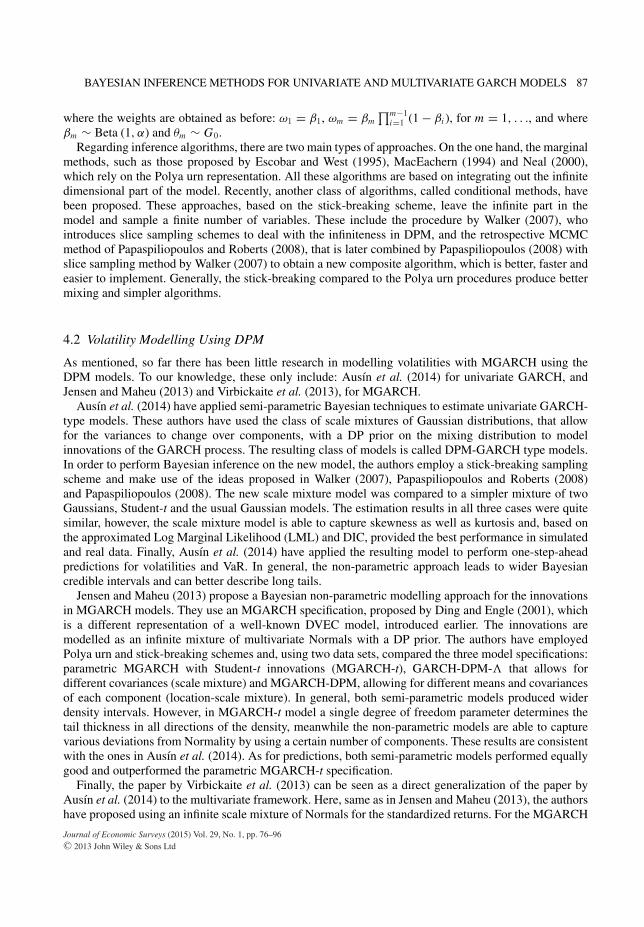
BAYESIAN INFERENCE METHODS FOR UNIVARIATE AND MULTIVARIATE GARCH MODELS 87
where the weights are obtained as before: ω1 = β1, ωm = βm∏m−1
i=1 (1 − βi ), for m = 1, . . ., and whereβm ∼ Beta (1, α) and θm ∼ G0.
Regarding inference algorithms, there are two main types of approaches. On the one hand, the marginalmethods, such as those proposed by Escobar and West (1995), MacEachern (1994) and Neal (2000),which rely on the Polya urn representation. All these algorithms are based on integrating out the infinitedimensional part of the model. Recently, another class of algorithms, called conditional methods, havebeen proposed. These approaches, based on the stick-breaking scheme, leave the infinite part in themodel and sample a finite number of variables. These include the procedure by Walker (2007), whointroduces slice sampling schemes to deal with the infiniteness in DPM, and the retrospective MCMCmethod of Papaspiliopoulos and Roberts (2008), that is later combined by Papaspiliopoulos (2008) withslice sampling method by Walker (2007) to obtain a new composite algorithm, which is better, faster andeasier to implement. Generally, the stick-breaking compared to the Polya urn procedures produce bettermixing and simpler algorithms.
4.2 Volatility Modelling Using DPM
As mentioned, so far there has been little research in modelling volatilities with MGARCH using theDPM models. To our knowledge, these only include: Ausın et al. (2014) for univariate GARCH, andJensen and Maheu (2013) and Virbickaite et al. (2013), for MGARCH.
Ausın et al. (2014) have applied semi-parametric Bayesian techniques to estimate univariate GARCH-type models. These authors have used the class of scale mixtures of Gaussian distributions, that allowfor the variances to change over components, with a DP prior on the mixing distribution to modelinnovations of the GARCH process. The resulting class of models is called DPM-GARCH type models.In order to perform Bayesian inference on the new model, the authors employ a stick-breaking samplingscheme and make use of the ideas proposed in Walker (2007), Papaspiliopoulos and Roberts (2008)and Papaspiliopoulos (2008). The new scale mixture model was compared to a simpler mixture of twoGaussians, Student-t and the usual Gaussian models. The estimation results in all three cases were quitesimilar, however, the scale mixture model is able to capture skewness as well as kurtosis and, based onthe approximated Log Marginal Likelihood (LML) and DIC, provided the best performance in simulatedand real data. Finally, Ausın et al. (2014) have applied the resulting model to perform one-step-aheadpredictions for volatilities and VaR. In general, the non-parametric approach leads to wider Bayesiancredible intervals and can better describe long tails.
Jensen and Maheu (2013) propose a Bayesian non-parametric modelling approach for the innovationsin MGARCH models. They use an MGARCH specification, proposed by Ding and Engle (2001), whichis a different representation of a well-known DVEC model, introduced earlier. The innovations aremodelled as an infinite mixture of multivariate Normals with a DP prior. The authors have employedPolya urn and stick-breaking schemes and, using two data sets, compared the three model specifications:parametric MGARCH with Student-t innovations (MGARCH-t), GARCH-DPM-� that allows fordifferent covariances (scale mixture) and MGARCH-DPM, allowing for different means and covariancesof each component (location-scale mixture). In general, both semi-parametric models produced widerdensity intervals. However, in MGARCH-t model a single degree of freedom parameter determines thetail thickness in all directions of the density, meanwhile the non-parametric models are able to capturevarious deviations from Normality by using a certain number of components. These results are consistentwith the ones in Ausın et al. (2014). As for predictions, both semi-parametric models performed equallygood and outperformed the parametric MGARCH-t specification.
Finally, the paper by Virbickaite et al. (2013) can be seen as a direct generalization of the paper byAusın et al. (2014) to the multivariate framework. Here, same as in Jensen and Maheu (2013), the authorshave proposed using an infinite scale mixture of Normals for the standardized returns. For the MGARCH
Journal of Economic Surveys (2015) Vol. 29, No. 1, pp. 76–96C© 2013 John Wiley & Sons Ltd
88 VIRBICKAITE ET AL.
020
040
060
080
010
0012
0014
0016
0018
0020
00
−10−
50510
FT
SE
100
Log−
Ret
urns
Log−Returns
020
040
060
080
010
0012
0014
0016
0018
0020
00
−10−
5051015
S&
P50
0 Lo
g−R
etur
ns
Log−Returns
−10
−8
−6
−4
−2
02
46
810
050100
150
200
250
300
350
FT
SE
100
His
togr
am
−10
−5
05
1015
050100
150
200
250
300
350
400
450
500
S&
P50
0 H
isto
gram
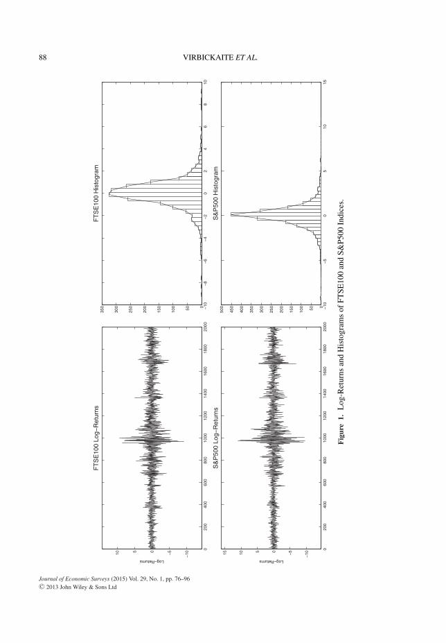
Fig
ure
1.L
og-R
etur
nsan
dH
isto
gram
sof
FTSE
100
and
S&P5
00In
dice
s.
Journal of Economic Surveys (2015) Vol. 29, No. 1, pp. 76–96C© 2013 John Wiley & Sons Ltd
BAYESIAN INFERENCE METHODS FOR UNIVARIATE AND MULTIVARIATE GARCH MODELS 89
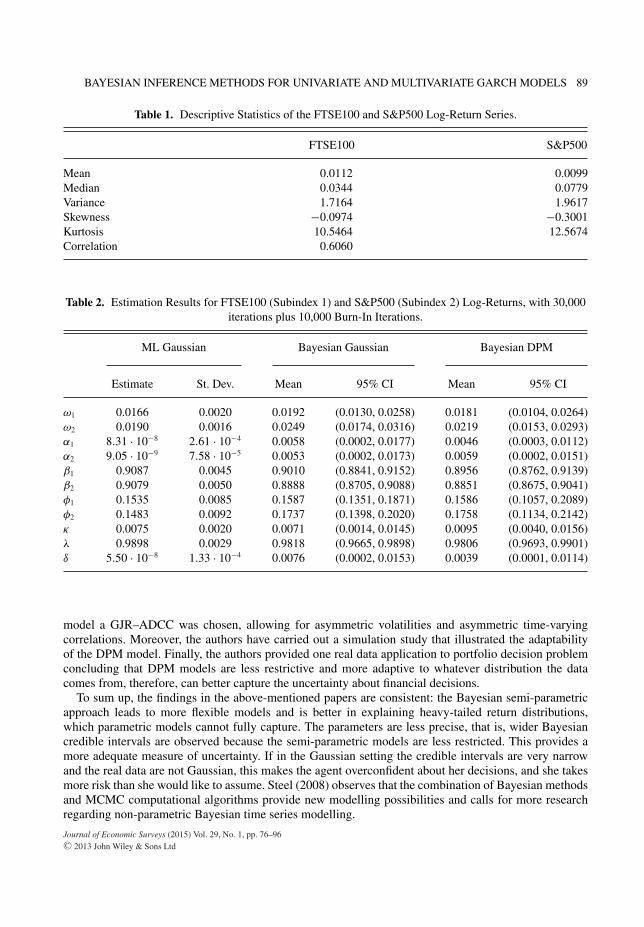
Table 1. Descriptive Statistics of the FTSE100 and S&P500 Log-Return Series.
FTSE100 S&P500
Mean 0.0112 0.0099Median 0.0344 0.0779Variance 1.7164 1.9617Skewness −0.0974 −0.3001Kurtosis 10.5464 12.5674Correlation 0.6060
Table 2. Estimation Results for FTSE100 (Subindex 1) and S&P500 (Subindex 2) Log-Returns, with 30,000iterations plus 10,000 Burn-In Iterations.
ML Gaussian Bayesian Gaussian Bayesian DPM
Estimate St. Dev. Mean 95% CI Mean 95% CI
ω1 0.0166 0.0020 0.0192 (0.0130, 0.0258) 0.0181 (0.0104, 0.0264)ω2 0.0190 0.0016 0.0249 (0.0174, 0.0316) 0.0219 (0.0153, 0.0293)α1 8.31 · 10−8 2.61 · 10−4 0.0058 (0.0002, 0.0177) 0.0046 (0.0003, 0.0112)α2 9.05 · 10−9 7.58 · 10−5 0.0053 (0.0002, 0.0173) 0.0059 (0.0002, 0.0151)β1 0.9087 0.0045 0.9010 (0.8841, 0.9152) 0.8956 (0.8762, 0.9139)β2 0.9079 0.0050 0.8888 (0.8705, 0.9088) 0.8851 (0.8675, 0.9041)φ1 0.1535 0.0085 0.1587 (0.1351, 0.1871) 0.1586 (0.1057, 0.2089)φ2 0.1483 0.0092 0.1737 (0.1398, 0.2020) 0.1758 (0.1134, 0.2142)κ 0.0075 0.0020 0.0071 (0.0014, 0.0145) 0.0095 (0.0040, 0.0156)λ 0.9898 0.0029 0.9818 (0.9665, 0.9898) 0.9806 (0.9693, 0.9901)δ 5.50 · 10−8 1.33 · 10−4 0.0076 (0.0002, 0.0153) 0.0039 (0.0001, 0.0114)
model a GJR–ADCC was chosen, allowing for asymmetric volatilities and asymmetric time-varyingcorrelations. Moreover, the authors have carried out a simulation study that illustrated the adaptabilityof the DPM model. Finally, the authors provided one real data application to portfolio decision problemconcluding that DPM models are less restrictive and more adaptive to whatever distribution the datacomes from, therefore, can better capture the uncertainty about financial decisions.
To sum up, the findings in the above-mentioned papers are consistent: the Bayesian semi-parametricapproach leads to more flexible models and is better in explaining heavy-tailed return distributions,which parametric models cannot fully capture. The parameters are less precise, that is, wider Bayesiancredible intervals are observed because the semi-parametric models are less restricted. This provides amore adequate measure of uncertainty. If in the Gaussian setting the credible intervals are very narrowand the real data are not Gaussian, this makes the agent overconfident about her decisions, and she takesmore risk than she would like to assume. Steel (2008) observes that the combination of Bayesian methodsand MCMC computational algorithms provide new modelling possibilities and calls for more researchregarding non-parametric Bayesian time series modelling.
Journal of Economic Surveys (2015) Vol. 29, No. 1, pp. 76–96C© 2013 John Wiley & Sons Ltd
90 VIRBICKAITE ET AL.
−3
−2
−1
01
23
−25
−20
−15
−10−
505
r 1,t+
1
DP
MN
orm
al
−3
−2
−1
01
23
−25
−20
−15
−10−
505
r 2,t+
1
DP
MN
orm
al
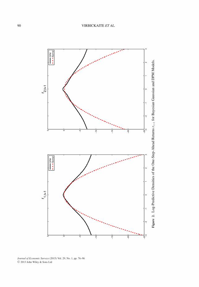
Fig
ure
2.L
og-P
redi
ctiv
eD
ensi
ties
ofth
eO
ne-S
tep-
Ahe
adR
etur
nsr t
+1fo
rB
ayes
ian
Gau
ssia
nan
dD
PMM
odel
s.
Journal of Economic Surveys (2015) Vol. 29, No. 1, pp. 76–96C© 2013 John Wiley & Sons Ltd
BAYESIAN INFERENCE METHODS FOR UNIVARIATE AND MULTIVARIATE GARCH MODELS 91
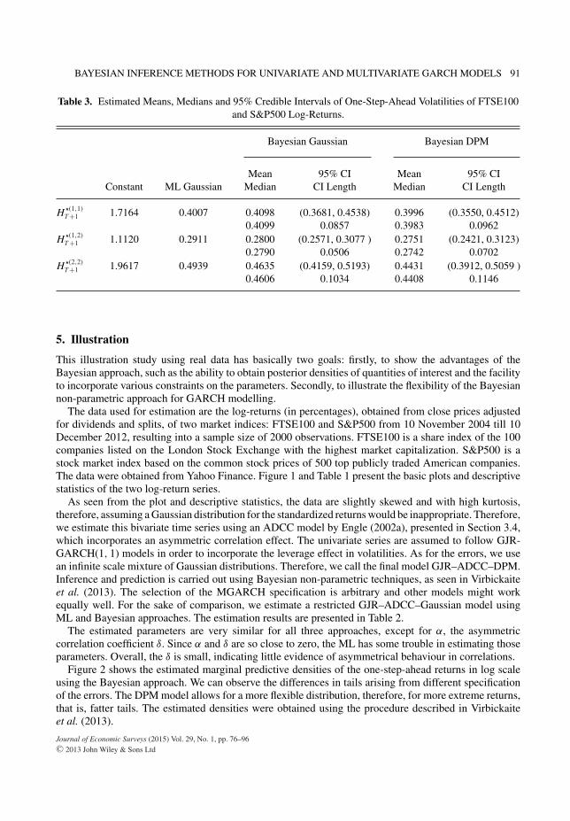
Table 3. Estimated Means, Medians and 95% Credible Intervals of One-Step-Ahead Volatilities of FTSE100and S&P500 Log-Returns.
Bayesian Gaussian Bayesian DPM
Mean 95% CI Mean 95% CIConstant ML Gaussian Median CI Length Median CI Length
H �(1,1)T +1 1.7164 0.4007 0.4098 (0.3681, 0.4538) 0.3996 (0.3550, 0.4512)
0.4099 0.0857 0.3983 0.0962H �(1,2)
T +1 1.1120 0.2911 0.2800 (0.2571, 0.3077 ) 0.2751 (0.2421, 0.3123)0.2790 0.0506 0.2742 0.0702
H �(2,2)T +1 1.9617 0.4939 0.4635 (0.4159, 0.5193) 0.4431 (0.3912, 0.5059 )
0.4606 0.1034 0.4408 0.1146
5. Illustration
This illustration study using real data has basically two goals: firstly, to show the advantages of theBayesian approach, such as the ability to obtain posterior densities of quantities of interest and the facilityto incorporate various constraints on the parameters. Secondly, to illustrate the flexibility of the Bayesiannon-parametric approach for GARCH modelling.
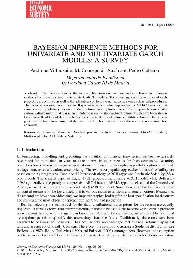
The data used for estimation are the log-returns (in percentages), obtained from close prices adjustedfor dividends and splits, of two market indices: FTSE100 and S&P500 from 10 November 2004 till 10December 2012, resulting into a sample size of 2000 observations. FTSE100 is a share index of the 100companies listed on the London Stock Exchange with the highest market capitalization. S&P500 is astock market index based on the common stock prices of 500 top publicly traded American companies.The data were obtained from Yahoo Finance. Figure 1 and Table 1 present the basic plots and descriptivestatistics of the two log-return series.
As seen from the plot and descriptive statistics, the data are slightly skewed and with high kurtosis,therefore, assuming a Gaussian distribution for the standardized returns would be inappropriate. Therefore,we estimate this bivariate time series using an ADCC model by Engle (2002a), presented in Section 3.4,which incorporates an asymmetric correlation effect. The univariate series are assumed to follow GJR-GARCH(1, 1) models in order to incorporate the leverage effect in volatilities. As for the errors, we usean infinite scale mixture of Gaussian distributions. Therefore, we call the final model GJR–ADCC–DPM.Inference and prediction is carried out using Bayesian non-parametric techniques, as seen in Virbickaiteet al. (2013). The selection of the MGARCH specification is arbitrary and other models might workequally well. For the sake of comparison, we estimate a restricted GJR–ADCC–Gaussian model usingML and Bayesian approaches. The estimation results are presented in Table 2.
The estimated parameters are very similar for all three approaches, except for α, the asymmetriccorrelation coefficient δ. Since α and δ are so close to zero, the ML has some trouble in estimating thoseparameters. Overall, the δ is small, indicating little evidence of asymmetrical behaviour in correlations.
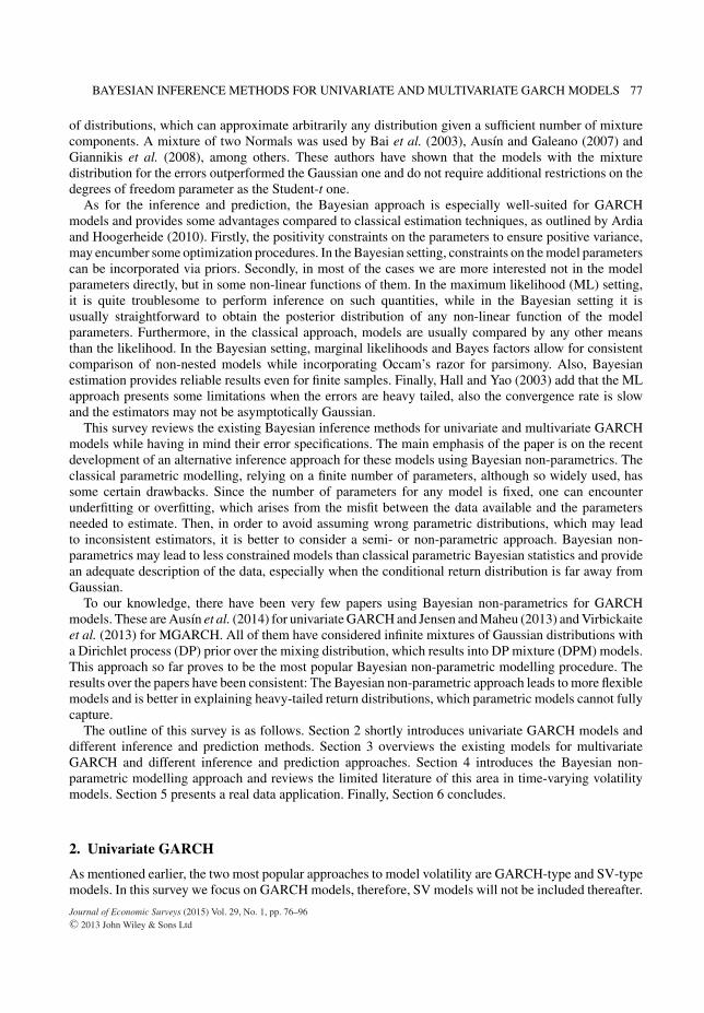
Figure 2 shows the estimated marginal predictive densities of the one-step-ahead returns in log scaleusing the Bayesian approach. We can observe the differences in tails arising from different specificationof the errors. The DPM model allows for a more flexible distribution, therefore, for more extreme returns,that is, fatter tails. The estimated densities were obtained using the procedure described in Virbickaiteet al. (2013).
Journal of Economic Surveys (2015) Vol. 29, No. 1, pp. 76–96C© 2013 John Wiley & Sons Ltd
92 VIRBICKAITE ET AL.
0.3
0.32
0.34
0.36
0.38
0.4
0.42
0.44
0.46
0.48
0.5
02468101214161820
(1,1
) of
Ht+
1*
DP
MG
auss
ian
ML
0.6
0.62
0.64
0.66
0.68
0.7
0102030405060
Cor
r t+1
*
DP
MG
auss
ian
ML
0.36
0.38
0.4
0.42
0.44
0.46
0.48
0.5
0.52
0.54
0.56
0246810121416
(2,2
) of
Ht+
1*
DP
MG
auss
ian
ML
Fig
ure
3.D
ensi
ties
ofO
ne-S
tep-
Ahe
adV
olat
ilitie
sof
the
Ret
urns
.
Journal of Economic Surveys (2015) Vol. 29, No. 1, pp. 76–96C© 2013 John Wiley & Sons Ltd
BAYESIAN INFERENCE METHODS FOR UNIVARIATE AND MULTIVARIATE GARCH MODELS 93
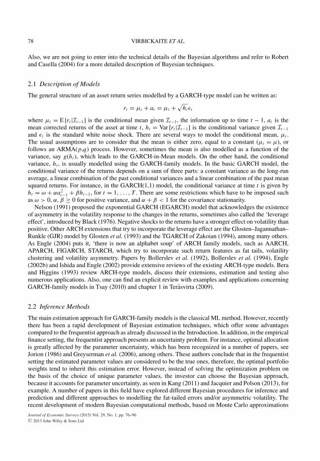
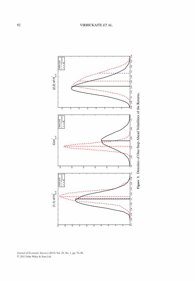
Table 3 presents the estimated mean, median and 95% credible intervals of one-step-ahead volatilitymatrices in Bayesian context. The matrix element (1,1) represents the volatility for the FTSE100 series(2,2) for the S&P500, and the elements in the diagonal (1,2) and (2,1) represent the covariance of bothfinancial returns. Figure 3 draws the posterior distributions for volatilities and correlation. The estimatedmean volatilities for both, DPM and Gaussian approaches, are very similar, however, the main differencesarise from the shape of the posterior distribution. Ninety-five percent credible intervals for DPM modelcorrelation are wider providing a more realistic measure of uncertainty about future correlations betweentwo assets. This is a very important implication in financial setting, because if an investor chooses to beGaussian, she would be overconfident about her decision and unable to adequately measure the risk sheis facing. See Virbickaite et al. (2013) for a more detailed comparison of DPM and alternative parametricapproaches in portfolio decision problems.
To sum up, this illustration has shown the main differences between the standard estimation proceduresand the new non-parametric approach. Even though the point estimates for the parameters and the one-step-ahead volatilities are very similar, the main differences arise from the thickness of tails of predictivedistributions of one-step-ahead returns and the shape of the posterior distribution for the one-step-aheadvolatilities.
6. Conclusions
In this paper, we reviewed univariate and multivariate GARCH models and inference methods, puttingemphasis on the Bayesian approach. We have surveyed the existing literature that concerns variousBayesian inference methods for MGARCH models, outlining the advantages of the Bayesian approachversus the classical procedures. We have also discussed in more detail the recent Bayesian non-parametricmethod for GARCH models, which avoid imposing arbitrary parametric distributional assumptions. Thisnew approach is more flexible and can describe better the uncertainty about future volatilities and returns,as has been illustrated using real data.
Acknowledgements
We are grateful to an anonymous referee for helpful comments. The first and second authors are grateful forthe financial support from MEC grant ECO2011-25706. The third author acknowledges financial support fromMEC grant ECO2012-38442.
References
Alexander, C.O. and Chibumba, A.M. (1997) Multivariate orthogonal factor GARCH. Mimeo, University ofSussex.
Antoniak, C.E. (1974) Mixtures of Dirichlet processes with applications to Bayesian nonparametric problems.Annals of Statistics 2: 1152–1174.
Arakelian, V. and Dellaportas, P. (2012) Contagion determination via copula and volatility threshold models.Quantitative Finance 12: 295–310.
Ardia, D. (2006) Bayesian estimation of the GARCH (1,1) model with normal innovations. Student 5: 1–13.Ardia, D. and Hoogerheide, L.F. (2010) Efficient Bayesian Estimation And Combination Of Garch-Type
Models. In K. Bocker (ed.), Rethinking Risk Measurement and Reporting: Examples and Applicationsfrom Finance: Vol II, , Chapter 1. London: RiskBooks.
Asai, M. (2006) Comparison of MCMC methods for estimating GARCH models. Journal of the Japan StatisticalSociety 36: 199–212.
Ausın, M.C. and Galeano, P. (2007) Bayesian estimation of the Gaussian mixture GARCH model.Computational Statistics & Data Analysis 51: 2636–2652.
Journal of Economic Surveys (2015) Vol. 29, No. 1, pp. 76–96C© 2013 John Wiley & Sons Ltd
94 VIRBICKAITE ET AL.
Ausın, M.C. and Lopes, H.F. (2010) Time-varying joint distribution through copulas. Computational Statistics& Data Analysis 54: 2383–2399.
Ausın, M.C., Galeano, P. and Ghosh, P. (2014) A semiparametric Bayesian approach to the analysis of financialtime series with applications to value at risk estimation. European Journal of Operational Research 232:350–358.
Bai, X., Russell, J.R. and Tiao, G.C. (2003) Kurtosis of GARCH and stochastic volatility models with non-normal innovations. Journal of Econometrics 114: 349–360.
Bauwens, L. and Lubrano, M. (1998) Bayesian inference on GARCH models using the Gibbs sampler.Econometrics Journal 1: 23–46.
Bauwens, L. and Lubrano, M. (2002) Bayesian option pricing using asymmetric GARCH models. Journal ofEmpirical Finance 9: 321–342.
Bauwens, L., Laurent, S. and Rombouts, J.V.K. (2006) Multivariate GARCH models: a survey. Journal ofApplied Econometrics 21: 79–109.
Bera, A.K. and Higgins, M.L. (1993) ARCH models: properties, estimation and testing. Journal of EconomicSurveys 7: 305–362.
Black, F. (1976) Studies of stock market volatility changes. Proceedings of the American Statistical Association;Business and Economic Statistics Section 177–181.
Bollerslev, T. (1986) Generalized autoregressive conditional heteroskedasticity. Journal of Econometrics 31:307–327.
Bollerslev, T. (1987) A conditionally heteroskedastic time series model for speculative prices and rates ofreturn. The Review of Economics and Statistics 69: 542–547.
Bollerslev, T. (1990) Modelling the coherence in short-run nominal exchange rates: a multivariate generalizedARCH model. The Review of Economics and Statistics 72: 498–505.
Bollerslev, T., Chou, R.Y. and Kroner, K.F. (1992) ARCH modeling in finance: a review of the theory andempirical evidence. Journal of Econometrics 52: 5–59.
Bollerslev, T., Engle, R.F. and Nelson, D.B. (1994) ARCH models. In R.F. Engle and D. McFadden (eds),Handbook of Econometrics, Vol. 4 (pp. 2959–3038). Amsterdam: Elsevier.
Bollerslev, T., Engle, R.F. and Wooldridge, J.M. (1988) A capital asset pricing model with time-varyingcovariances. Journal of Political Economy 96: 116–131.
Burda, M. (2013) Constrained Hamiltonian Monte Carlo in BEKK GARCH with targeting. Working Paper,University of Toronto.
Burda, M. and Maheu, J.M. (2013) Bayesian adaptively updated Hamiltonian Monte Carlo with an application tohigh-dimensional BEKK GARCH models. Studies in Nonlinear Dynamics & Econometrics17: 345–372.
Cappiello, L., Engle, R.F. and Sheppard, K. (2006) Asymmetric dynamics in the correlations of global equityand bond returns. Journal of Financial Econometrics 4: 537–572.
Chen, C.W., Gerlach, R. and So, M. K. (2009) Bayesian model selection for heteroscedastic models. Advancesin Econometrics 23: 567–594.
Dellaportas, P. and Vrontos, I.D. (2007) Modelling volatility asymmetries: a Bayesian analysis of a class oftree structured multivariate GARCH models. The Econometrics Journal 10: 503–520.
Ding, Z. and Engle, R.F. (2001) Large scale conditional covariance matrix modeling, estimation and testing.Academia Economic Papers 29: 157–184.
Engle, R.F. (1982) Autoregressive conditional heteroskedasticity with estimates of the variance of UnitedKingdom inflation. Econometrica 50: 987–1008.
Engle, R.F. (2002a) Dynamic conditional correlation. Journal of Business & Economic Statistics 20: 339–350.Engle, R.F. (2002b) New frontiers for ARCH models. Journal of Applied Econometrics 17: 425–446.Engle, R.F. (2004) Risk and volatility: econometric models and financial practice. The American Economic
Review 94: 405–420.Engle, R.F. and Kroner, K.F. (1995) Multivariate simultaneous generalized ARCH. Econometric Theory 11:
122–150.Engle, R.F., Ng, V.K. and Rothschild, M. (1990) Asset pricing with a factor-ARCH covariance structure.
Journal of Econometrics 45: 213–237.Escobar, M.D. and West, M. (1995) Bayesian density estimation and inference using mixtures. Journal of the
American Statistical Association 90: 577–588.
Journal of Economic Surveys (2015) Vol. 29, No. 1, pp. 76–96C© 2013 John Wiley & Sons Ltd
BAYESIAN INFERENCE METHODS FOR UNIVARIATE AND MULTIVARIATE GARCH MODELS 95
Ferguson, T.S. (1973) A Bayesian analysis of some nonparametric problems. Annals of Statistics 1: 209–230.Galeano, P. and Ausın, M.C. (2010) The Gaussian mixture dynamic conditional correlation model: parameter
estimation, value at risk calculation, and portfolio selection. Journal of Business and Economic Statistics28: 559–571.
Geweke, J. (1992) Evaluating the accuracy of sampling-based approaches to the calculation of posteriormoments. Bayesian Statistics 4: 169–193.
Giannikis, D., Vrontos, I.D. and Dellaportas, P. (2008) Modelling nonlinearities and heavy tails via thresholdnormal mixture GARCH models. Computational Statistics & Data Analysis 52: 1549–1571.
Gilks, W.R., Best, N.G. and Tan, K.K.C. (1995) Adaptive rejection metropolis sampling within Gibbs sampling.Journal of the Royal Statistical Society Series C 44: 455–472.
Glosten, L.R., Jagannathan, R. and Runkle, D.E. (1993) On the relation between the expected value and thevolatility of the nominal excess return on stocks. The Journal of Finance 48: 1779–1801.
Greyserman, A., Jones, D.H. and Strawderman, W.E. (2006) Portfolio selection using hierarchical Bayesiananalysis and MCMC methods. Journal of Banking & Finance 30: 669–678.
Hall, P. and Yao, Q. (2003) Inference in ARCH and GARCH models with heavy-tailed errors. Econometrica71: 285–317.
He, C. and Terasvirta, T. (1999) Properties of moments of a family of GARCH processes. Journal ofEconometrics 92: 173–192.
Hofmann, M. and Czado, C. (2010) Assessing the VaR of a portfolio using D-vine copula based multivariateGARCH models. Working Paper, Technische Universitat Munchen Zentrum Mathematik.
Hudson, B.G. and Gerlach, R.H. (2008) A Bayesian approach to relaxing parameter restrictions in multivariateGARCH models. Test 17: 606–627.
Ishida, I. and Engle, R.F. (2002) Modeling variance of variance: the square-root, the affine, and the CEVGARCH models. Working Paper, New York University, pp. 1–47.
Jacquier, E. and Polson, N.G. (2013) Asset allocation in finance: a Bayesian perspective. In P. Damien,P. Dellaportas, N.G. Polson and D.A. Stephen (eds), Bayesian Theory and Applications, (pp. 501–516).Oxford: Oxford University Press.
Jensen, M.J. and Maheu, J.M. (2013) Bayesian semiparametric multivariate GARCH modeling. Journal ofEconometrics 176: 3–17.
Jin, X. and Maheu, J.M. (2013) Modeling realized covariances and returns. Journal of Financial Econometrics11: 335–369.
Jorion, P. (1986) Bayes-stein estimation for portfolio analysis. The Journal of Financial and QuantitativeAnalysis 21: 279–292.
Kang, L. (2011) Asset allocation in a Bayesian copula-GARCH framework: an application to the ‘passive fundsversus active funds’ problem. Journal of Asset Management 12: 45–66.
Kim, S., Shephard, N. and Chib, S. (1998) Stochastic volatility: likelihood inference and comparison withARCH Models. Review of Economic Studies 65: 361–393.
Lin, W.L. (1992) Alternative estimators for factor GARCH models: a Monte Carlo comparison. Journal ofApplied Econometrics 7: 259–279.
MacEachern, S.N. (1994) Estimating normal means with a conjugate style Dirichlet process prior.Communications in Statistics: Simulation and Computation 23: 727–741.
Miazhynskaia, T. and Dorffner, G. (2006) A comparison of Bayesian model selection based on MCMC withapplication to GARCH-type models. Statistical Papers 47: 525–549.
Muller, P. and Pole, A. (1998) Monte Carlo posterior integration in GARCH models. Sankhya, Series B 60:127–14.
Nakatsuma, T. (2000) Bayesian analysis of ARMA-GARCH models: a Markov chain sampling approach.Journal of Econometrics 95: 57–69.
Neal, R.M. (2000) Markov chain sampling methods for Dirichlet process mixture models. Journal ofComputational and Graphical Statistics 9: 249–265.
Nelson, D.B. (1991) Conditional heteroskedasticity in asset returns: a new approach. Econometrica 59: 347–370.
Osiewalski, J. and Pipien, M. (2004) Bayesian comparison of bivariate ARCH-type models for the mainexchange rates in Poland. Journal of Econometrics 123: 371–391.
Journal of Economic Surveys (2015) Vol. 29, No. 1, pp. 76–96C© 2013 John Wiley & Sons Ltd
96 VIRBICKAITE ET AL.
Papaspiliopoulos, O. (2008) A note on posterior sampling from Dirichlet mixture models. Working Paper,University of Warwick. Centre for Research in Statistical Methodology, Coventry, pp. 1–8.
Papaspiliopoulos, O. and Roberts, G.O. (2008). Retrospective Markov chain Monte Carlo methods for Dirichletprocess hierarchical models. Biometrika 95: 169–186.
Patton, A.J. (2006) Modelling asymmetric exchange rate dependence. International Economic Review 47:527–556.
Patton, A.J. (2009) Copula-based models for financial time series. In T.G. Andersen, T. Mikosch, J.P. Kreiß,and R.A. Davis (eds), Handbook of Financial Time Series, Chapter 36, (pp. 767–785). Berlin, Heidelberg:Springer.
Robert, C.P. and Casella, G. (2004) Monte Carlo Statistical Methods. Springer Texts in Statistics, 2nd edn. NewYork: Springer.
Silvennoinen, A. and Terasvirta, T. (2009) Multivariate GARCH models. In T.G. Andersen, T. Mikosch, J.P.Kreiß, and R.A. Davis (eds), Handbook of Financial Time Series, (pp. 201–229). Berlin, Heidelberg:Springer.
Sklar, A. (1959) Fonctions de repartition a n dimensions et leur marges. Publications de l’Institut de Statistiquede l’Universite de Paris. 8: 229–231.
Steel, M. (2008) Bayesian time series analysis. In S. Durlauf and L. Blume (eds), The New Palgrave Dictionaryof Economics, 2nd edn. London: Palgrave Macmillan.
Terasvirta, T. (2009) An introduction to univariate GARCH models. In T.G. Andersen, T. Mikosch, J.P. Kreiß,and R.A. Davis (eds), Handbook of Financial Time Series, (pp. 17–42). Berlin, Heidelberg: Springer.
Tierney, L. (1994) Markov chains for exploring posterior distributions. Annals of Statistics 22: 1701–1728.Tsay, R.S. (2010) Analysis of Financial Time Series, 3rd edn. Hoboken: John Wiley & Sons, Inc.Tse, Y.K. and Tsui, A.K.C. (2002) A multivariate generalized autoregressive conditional heteroscedasticity
model with time-varying correlations. Journal of Business & Economic Statistics 20: 351–362.Van der Weide, R. (2002) GO-GARCH: a multivariate generalized orthogonal GARCH model. Journal of
Applied Econometrics 17: 549–564.Virbickaite, A., Ausın, M.C. and Galeano, P. (2013) A Bayesian non-parametric approach to asymmet-
ric dynamic conditional correlation model with application to portfolio selection. Working paper,arXiv:1301.5129v1 [q-fin.PM]
Vrontos, I.D., Dellaportas, P. and Politis, D.N. (2000) Full Bayesian inference for GARCH and EGARCHmodels. Journal of Business and Economic Statistics 18: 187–198.
Vrontos, I.D., Dellaportas, P. and Politis, D.N. (2003a) A full-factor multivariate GARCH model. EconometricsJournal 6: 312–334.
Vrontos, I.D., Dellaportas, P. and Politis, D.N. (2003b) Inference for some multivariate ARCH and GARCHmodels. Journal of Forecasting 22: 427–446.
Wago, H. (2004) Bayesian estimation of smooth transition GARCH model using Gibbs sampling. Mathematicsand Computers in Simulation 64: 63–78.
Walker, S.G. (2007) Sampling the Dirichlet mixture model with slices. Communications in Statistics: Simulationand Computation 36: 45–54.
Yu, B. and Mykland, P. (1998) Looking at Markov samplers through cusum path plots: a simple diagnosticidea. Statistics and Computing 8: 275–286.
Zakoian, J.M. (1994) Threshold heteroskedastic models. Journal of Economic Dynamics and Control 18:931–955.
Journal of Economic Surveys (2015) Vol. 29, No. 1, pp. 76–96C© 2013 John Wiley & Sons Ltd
Related Documents