Discrete all-pole modeling - Signal Processing, IEEE Transactions on

I

IEEE TRANSACTIONS ON SIGNAL PROCESSING, VOL. 39, NO. 2, FEBRUARY 1991

Discrete All-Pole Modeling Amro El-Jaroudi, Member, IEEE, and John Makhoul, Fellow, IEEE

Abstract-A new method is introduced for parametric modeling of spectral envelopes when only a discrete set of spectral points is given. This method, which we call discrete all-pole (DAP) modeling, uses a discrete version of the Itakura-Saito distortion measure as its error criterion. One result is a new autocorrelation matching condition that overcomes the limitations of linear prediction and produces better fitting spectral envelopes for spectra that are representable by a rela- tively small discrete set of values, such as in voiced speech.

We present an iterative algorithm for DAP modeling that is shown to converge to a unique global minimum. We also present results of applying DAP modeling to real and synthetic speech. DAP modeling is extended to allow frequency-dependent weighting of the error measure, so that spectral accuracy can be enhanced in certain frequency regions relative to others.

1. INTRODUCTION POPULAR approach to speech modeling is to use a time- A varying all-pole spectral shaping filter with a variable ex-

citation source. This all-pole filter is typically estimated using linear prediction methods [ 111. It has been known for some time that linear prediction (LP) suffers from drawbacks that are especially manifested during voiced segments of speech. Specif- ically, the peaks of LP spectral estimates during these segments are highly biased towards the pitch harmonics, especially for high-pitched sounds and voices [ 111. It has been pointed out that the drawbacks of LP are inherent to its error criterion [ 1 1 1. To overcome these drawbacks, we propose in this paper a new all-pole modeling method based on a discrete form of the Ita- kura-Saito distance measure.

The new method, which we call discrete all-pole (DAP) modeling, overcomes the well-known limitations of LP and generally gives better all-pole spectral envelopes that are less biased towards the pitch harmonics. In DAP, we approximate the spectrum of voiced speech, which has its energy located approxi- mately at the harmonics of the fundamental pitch, by a line (discrete) spectrum. The problem of finding the spectral envelope is then reduced to fitting an all-pole spectrum to a finite set of spectral points so as to minimize the discrete form of the Itakura-Saito (I-S) distance measure. We present an algorithm to compute the optimal envelopes and show that DAP modeling produces generally better fitting spectral envelopes than LP.

Another advantage of DAP modeling is that the method can be extended to allow error weighting as a function of frequency. This weighting can be used to emphasize the spectral fit in sections of the spectrum at the expense of the fit at other sections. This method has known applications in various aspects of speech processing where better spectral accuracy is often desired at lower frequencies relative to high frequencies.

Manuscript received November 21, 1988; revised December 11, 1989.

A. El-Jaroudi is with the Department of Electrical Engineering, Univer-

J . Makhoul is with Bolt Beranek and Newman Inc., Cambridge, MA

IEEE Log Number 9041 149.

This work was supported in part by the Department of Defense.

sity of Pittsburgh, Pittsburgh, PA 15261.

02138.

41 1

In the next section, we present the known limitations of linear prediction. In Section 111, we introduce DAP modeling and derive the minimization conditions for the discrete form of the I-S distance measure. We also examine the possible forms of solutions one obtains using DAP modeling. In Section IV, we derive an iterative algorithm to compute the optimal all-pole model and discuss its convergence properties. The results of applying DAP modeling to various signals are presented in Sec- tion V. In Section VI, we modify DAP modeling to allow weighting of the error measure as a function of frequency, and the results of weighted DAP are compared to those without weighting.

11. LIMITATIONS OF LINEAR PREDICTIONS

In this section, we review linear prediction spectral analysis and demonstrate, using examples, some of its inherent limitations.

The basic concept of linear prediction (LP) is to predict, sub- ject to an error criterion, the present value of a signal based on its previousp values, wherep is the prediction order. Normally, the error criterion used is a least squares distance measure between the actual and predicted values. In the frequency domain, for discrete spectra defined at a set of frequencies U , E Q, the LP error criterion is equivalent to minimizing [ 121

where P( 0 ) is the spectrum of th,e given signal, N is the number of discrete frequencies U,, and P ( U ) is the spectrum of the all- pole envelope defined as

Note that, in the definition of P ( w ) , we have incorporated the gain factor in the coefficients of the denominator, i.e., a. is not restricted to 1. We emphasize here that the frequencies U , in the set Q, which includes both positive and negative frequencies, can be arbitrary and need not be equally spaced.

The minimization of ELp with respect to the predictor coefficients, ak, 1 5 k I p , yields a well-known set of normal equations:

P

k = O C R ( i - k)ak = 0, 1 5 i 5 p ( 3 )

and P 1

k=O a0 R(k)Uk = - (4)

( 5 )

1053-587X/91/0200-0411$01.00 0 1991 IEEE

412 IEEE TRANSACTIONS ON SIGNAL PROCESSING, VOL. 39, NO. 2, FEBRUARY 1991

is the autocorrelation of the discrete signal spectrum P ( U,). Equation (4) was obtained by substituting (3) in (1) and setting the energy of the continuous LP spectrum equal to the energy R (0) of the given discrete spectrum.

It is well known [ 111 that by minimizing ELP, we are matching the autocorrelation of the continuous LP envelope to that of the given discrete spectrum. In other words, we are effectively setting

where

and R ( i ) is the autocorrelation of the discrete spectrum in (5). In the following example, we show a typical behavior of LP

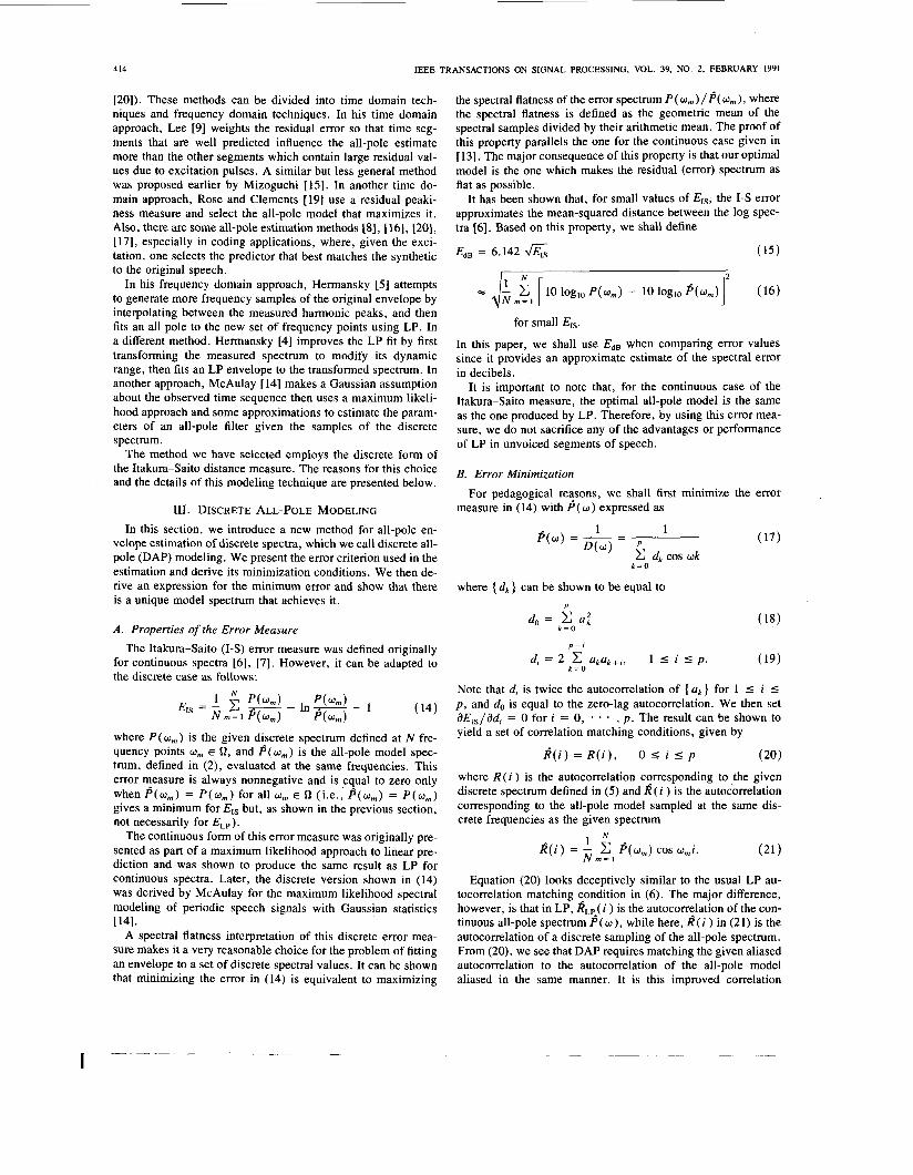
spectral analysis of discrete or harmonic spectra. We will use LP to attempt to recover the original all-pole envelope of a periodic signal. The spectral envelope shown in solid line in'Fig. l(a) represents a synthesis all-pole ( p = 12) filter which, when excited with a periodic pulse sequence having a discrete spectrum with N = 30 frequency points, will give a periodic signal whose line spectrum is shown in the figure. If we perform LP analysis on the periodic signal, we obtain the dashed envelope shown in Fig. l(a). Clearly, the LP envelope does not match the original envelope nor does it fit the discrete spectrum. While there is a unique all-pole envelope (the original) that perfectly fits the discrete spectrum, LP fails to recover that all-pole envelope. It has been shown [12] that for discrete spectra the LP error measure (1) possessss an error cancellation property which makes it select an envelope other than the only one which passes through all the spectral points.

We now show that it would be unreasonable to expect LP to recover the original envelope from the discrete spectral samples. We define Rorg to be the autocorrelation corresponding to the original all-pole filter with spectrum P( U ) . Rorg ( i ) and P ( w ) are related by the standard transform pair

and m

P ( O ) = C R , ~ ~ ( I ) e-]"'. (9) I= - m

The autocorrelation R corresponding to the discrete samples of the synthesis envelope is defined in (5). By substituting (9) in (3, we find that R is related to R,, by

, for all i. (IO) R ( i ) = - c R o r g ( I ) e-Jutf1( ' - ' )

This equation shows the aliasing that occurs in the autocorrelation domain whenever a spectral envelope is sampled at a discrete set of frequencies. For the periodic excitation case, the frequencies w, will be equally spaced at U, = 27r(m - l ) /N, and (10) reduces to

l N N m = ! I = - m

m

R ( i ) = Rorg( i - I N ) , for all i. (11)

For the example above, we show, in Figs. l(b) and (c), Rorg( i ) and R ( i ) for lags 0 I i 5 75 and excitation period N = 30. Note that R ( i ) as obtained by aliasing Rorg ( i ) as given by (1 1).

[ = - m

i

1

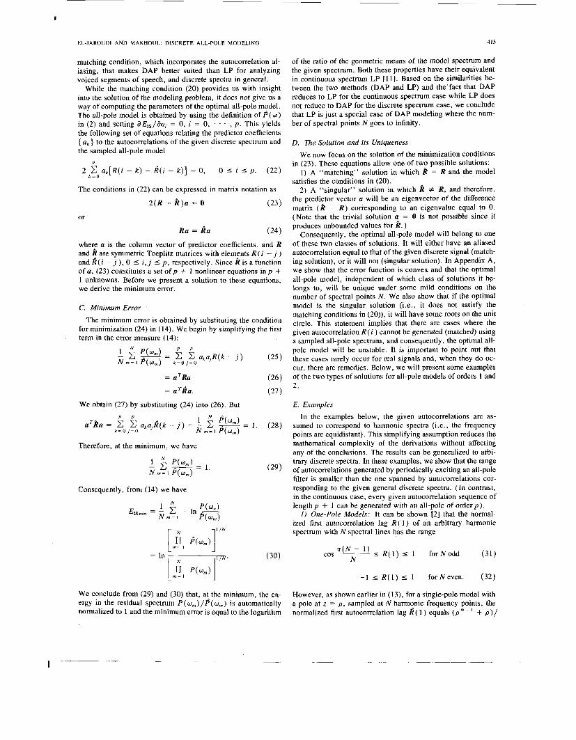
Fig. 1. (a) Example of the limitations of linear prediction spectral analysis. The solid line is the original 12-pole envelope which goes through all the points. The dashed line is the 12-pole LP model for N = 30 spectral lines. (b) Rorg ( i ) for lags 0 5 i 5 75 and excitation period N = 30. (c) Autocorrelation R ( i ), 0 c i 5 75, corresponding to the discrete spectrum in Fig. l(a). (d) Autocorrelation RLP(i), 0 5 i I 75, corresponding to the LP envelope in Fig. I(a). (e ) Discrete frequency sampled impulse response h( i ), -37 I i I 37 corresponding to the discrete spectrum in Fig. I@).

I

EL-JAROUDI AND MAKHOUL: DISCRETE ALL-POLE MODELING 413

As shown in (6 ) , LP matches the autocorrelation of the continuous model spectrum to that of the given spectrum. By applying this matching to the example shown above, we obtain

In other words, since the autocorrelation corresponding to the LP envelope will always equal an aliased version of Rorg (for the discrete spectrum case), the LP envelope will not equal the original envelope. It is also important to note that LP produces a unique all-pole model given a set of autocorrelations, which means that the original all pole is not a possible solution to (3). The autocorrelation R,, ( i ), 0 I i s 75, corresponding to the LP envelope in the example above is shown in Fig. l(d). We note that RLp( i ) in Fig. l(d) is equal to R( i ) in Fig. l(c) for the first 13 lags (since p = 12) and, very importantly, that RLP ( i ) is very different from the original autocorrelation Rorg shown in Fig. l(b). The LP error criterion matches the autocorrelation of the continuous all-pole model to the autocorrelation of the given signal without taking into account the aliasing that has occurred in the discrete spectrum. This interpretation of LP spectral estimation explains the sensitivity of LP estimates to high-pitched sounds. As the pitch increases, we have fewer and fewer harmonics (spectral samples) and the autocorrelation aliasing becomes more and more severe, which in turn, leads to worse LP models.

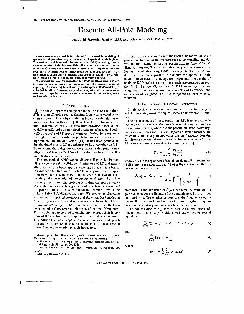
In Fig. 2(a), we show the same example as in Fig. 1 for N = 30 and nonperiodic excitation. The discrete spectral lines shown in the figure are not equidistant and are not multiples of some fundamental frequency. The original envelope is shown in solid line and the LP envelope in dashed. Once again, LP fails to recover the original envelope. It is easy to understand why the LP estimate was so poor by examining the autocorrelations corresponding to the original envelope and the discrete spectrum. These autocorrelations are shown in Fig. 2(b) and (c), respectively. We note how very different the aliased autocorrelation is from the original one. Consequently, the LP envelope whose autocorrelation is shown in Fig. 2(d) and is equal to the aliased autocorrelation for the first 13 lags, will also be very different from the original one. These examples show that LP is the wrong approach to envelope estimation for discrete spectra since it does not account for the aliasing caused by spectral sampling (periodic or nonperiodic).

This disregard to autocorrelation aliasing is demonstrated again in the following one-pole example. Given a single pole filter, with a real pole at z = p , excited by a periodic sequence with period N , one can show [2] that the resulting signal will have a normalized first autocorrelation lag R ( 1 ), given by

When we perform LP analysis on the periodic signal, the resulting one-pole LP envelope will have a pole at z = pLp = R ( l ) = ( p N - ' + p)/(l + p N ) . Forp = 0.95 and N = 10, for example, we have pLp = 0.99. Clearly, the LP envelope will have a much narrower bandwidth than the original one. We note from (13) that, as N gets larger, R( l ) , and hence pLp, will approach p , which as N + 03 corresponds to the continuous spectrum case. However, for many applications, especially for high- pitched speech, as N decreases, LP autocorrelation matching

Fig. 2 . (a) Example of the limitations of linear prediction spectral analysis for nonperiodic but discrete spectra. The solid line is the original 12-pole envelope; t& dashed line is the 12-pole LP model for N = 30 spectral lines. (b) Rocg( i ) for lags 0 5 i 5 75 corresponding to the solid envelope in Fig. 2(a). (c) Autocorrelation R ( i ), 0 5 i I 75, corresponding to the discrete spectrum-in Fig. 2(a) with N = 30 nonharmonic spectral lines. (d) Autocorrelation RLP( i), 0 5 i I 75, corresponding to the LP envelope in Fig. 2(a).

often produces suboptimal and inadequate results. This matching is forced upon us by the error measure used for LP.

To improve upon the LP estimate, researchers have devised methods with either a different error criterion or with added constraints to regular LP (e.g., [4], 151, [8], [9], [15]-1171,

414

[20]). These methods can be divided into time domain techniques and frequency domain techniques. In his time domain approach, Lee [9] weights the residual error so that time segments that are well predicted influence the all-pole estimate more than the other segments which contain large residual values due to excitation pulses. A similar but less general method was proposed earlier by Mizoguchi [15]. In another time domain approach, Rose and Clements [19] use a residual peaki- ness measure and select the all-pole model that maximizes it. Also, there are some all-pole estimation methods [ 81, [ 161, 1201, [ 171, especially in coding applications, where, given the excitation, one selects the predictor that best matches the synthetic to the original speech.

In his frequency domain approach, Hermansky [5] attempts to generate more frequency samples of the original envelope by interpolating between the measured harmonic peaks, and then fits an all pole to the new set of frequency points using LP. In a different method, Hermansky [4] improves the LP fit by first transforming the measured spectrum to modify its dynamic range, then fits an LP envelope to the transformed spectrum. In another approach, McAulay [ 141 makes a Gaussian assumption about the observed time sequence then uses a maximum likelihood approach and some approximations to estimate the parameters of an all-pole filter given the samples of the discrete spectrum.

The method we have selected employs the discrete form of the Itakura-Saito distance measure. The reasons for this choice and the details of this modeling technique are presented below.

IEEE TRANSACTIONS ON SIGNAL PROCESSING, VOL. 39, NO. 2, FEBRUARY 1991

111. DISCRETE ALL-POLE MODELING In this section, we introduce a new method for all-pole en-

velope estimation of discrete spectra, which we call discrete all- pole (DAP) modeling. We present the error criterion used in the estimation and derive its minimization conditions. We then derive an expression for the minimum error and show that there is a unique model spectrum that achieves it.

A. Properties of the Error Measure

The Itakura-Saito (I-S) error measure was defined originally for continuous spectra [6], [7]. However, it can be adapted to the discrete case as follows:

where P ( w , ) is the given discrete spectrum defined at N frequency points a, E Q, and P ( w , ) is the all-pole model spectrum, defined in (2), evaluated at the same frequencies. This error measure is always nonnegative and is equal to zero only when P(w,) = P(w,) for all w, E Q (i.e., P(w,) = P ( w , ) gives a minimum for E,, but, as shown in the previous section, not necessarily for E L p ) .

The continuous form of this error measure was originally presented as part of a maximum likelihood approach to linear prediction and was shown to produce the same result as LP for continuous spectra. Later, the discrete version shown in (14) was derived by McAulay for the maximum likelihood spectral modeling of periodic speech signals with Gaussian statistics

A spectral flatness interpretation of this discrete error measure makes it a very reasonable choice for the problem of fitting an envelope to a set of discrete spectral values. It can be shown that minimizing the error in (14) is equivalent to maximizing

~ 4 1 .

the spectral flatness of the error spectrum P ( w , ) / p ( w , ) , where the spectral flatness is defined as the geometric mean of the spectral samples divided by their arithmetic mean. The proof of this property parallels the one for the continuous case given in [ 131. The major consequence of this property is that our optimal model is the one which makes the residual (error) spectrum as flat as possible.

It has been shown that, for small values of EIS, the I-S error approximates the mean-squared distance between the log spectra [6]. Based on this property, we shall define

EdB = 6.142 (15)

for small EIS.

In this paper, we shall use EdB when comparing error values since it provides an approximate estimate of the spectral error in decibels.

It is important to note that, for the continuous case of the Itakura-Saito measure, the optimal all-pole model is the same as the one produced by LP. Therefore, by using this error measure, we do not sacrifice any of the advantages or performance of LP in unvoiced segments of speech.

B. Error Minimization

measure in (14) with P ( o ) expressed as For pedagogical reasons, we shall first minimize the error

k = O

where { d k } can be shown to be equal to P

do = c a: k = O

P-'

di = 2 c a k a k + i r 1 I i 5 p . (19) k = O

Note that d , is twice the autocorrelation of { a k } for 1 I i 5 p , and do is equal to the zero-lag autocorrelation. We then set aE, , /ad i = 0 for i = 0, * - , p . The result can be shown to yield a set of correlation matching conditions, given by

k ( i ) = R ( i ) , 0 I i 5 p (20)

where R ( i ) is the autocorrelation corresponding to the given discrete spectrum defined in (5) and R ( i ) is the autocorrelation corresponding to the all-pole model sampled at the same discrete frequencies as the given spectrum

. N

Equation (20) looks deceptively similar to the usual LP autocorrelation matching condition in (6). The major difference, however, is that in LP, RLpJi ) is the autocorrelation of the continuous all-pole spectrum P( a), while here, R ( i ) in (21) is the autocorrelation of a discrete sampling of the all-pole spectrum. From (20), we see that DAP requires matching the given aliased autocorrelation to the autocorrelation of the all-pole model aliased in the same manner. It is this improved correlation

I

EL-JAROUDI AND MAKHOUL: DISCRETE ALL-POLE MODELING

matching condition, which incorporates the autocorrelation aliasing, that makes DAP better suited than LP for analyzing voiced segments of speech, and discrete spectra in general.

While the matching condition (20) provides us with insight into the solution of the modeling problem, it does not give us a way of computing the parameters of the optimal all-pole model. The all-pole model is obtained by using the definition of P ( CO) in (2) and setting aE, , /aa , = 0, i = 0, * . . , p. This yields the following set of equations relating the predictor coefficients { ak } to the autocorrelations of the given discrete spectrum and the sampled all-pole model

P

2 c u k [ R ( i - k ) - k ( i - k ) ] = 0, 0 5 i 5 p. (22) k = O

The conditions in (22) can be expressed in matrix notation as

2(R - h ) a = 0 (23)

Ra = Ra (24)

or

whey U is the column vector of predictor coeficients, and R and R are symmetric Toeplitz matrices with elemfnts R ( i - j ) and R ( i - j ), 0 5 i , j 5 p, respectively. Since R is a function of a, (23) constitutes a set of p + 1 nonlinear equations in p f 1 unknowns. Before we present a solution to these equations, we derive the minimum error.

C. Minimum Error

The minimum error is obtained by substituting the condition for minimization (24) in (14). We begin by simplifying the first term in the error measure (14):

P P - c - - - C a,u,R(k - j ) N m = l P(w,) , = o j = o

= aTRa

= a’Ra.

We obtain (27) by substituting (24) into (26). But

1 P ( m m ) - P P

a’Ra = c c u,ujR(k - j ) = - c - - k = O j = O Nm=l P(w,)

Therefore, at the minimum, we have

Consequently, from (14) we have

L m = I J

L _I

We conclude from (29) and (30) that, at, the minimum, the energy in the residual spectrum P ( w,)/P( CO,) is automatically normalized to 1 and the minimum error is equal to the logarithm

415

of the ratio of the geometric means of the model spectrum and the given spectrum. Both these properties have their equivalent in continuous spectrum LP [ 111, Based on the similarities between the two methods (DAP and LP) and the‘fact that DAP reduces to LP for the continuous spectrum case while LP does not reduce to DAP for the discrete spectrum case, we conclude that LP is just a special case of DAP modeling where the number of spectral points N goes to infinity.

D. The Solution and its Uniqueness We now focus on the solution of the minimization conditions

in (23). These equations allow one of two possible solutions: 1) A “matching” solution in which R = R and the model

satisfies the conditions in (20). 2) A “singular” solution in which # R, and therefore,

the predictor vector a will be an eigenvector of the difference matrix ( R - R) corresponding to an eigenvalue equal to 0. (Note that the trivial solution a, = 0 is not possible since it produces unbounded values for R. )

Consequently, the optimal all-pole model will belong to one of these two classes of solutions. It will either have an aliased autocorrelation equal to that of the given discrete signal (matching solution), or it will not (singular solution). In Appendix A, we show that the error function is convex and that the optimal all-pole model, independent of which class of solutions it be- longs to, will be unique under some mild conditions on the number of spectral points N . We also show that if the optimal model is the singular solution (i.e., it does not satisfy the matching conditions in (20)), it will have some roots on the unit circle. This statement implies that there are cases where the given autocorrelation R(i ) cannot be generated (matched) using a sampled all-pole spectrum, and consequently, the optimal all- pole model will be unstable. It is important to point out that these cases rarely occur for real signals and, when they do occur, there are remedies. Below, we will present some examples of the two types of solutions for all-pole models of orders 1 and 2.

E. Examples In the examples below, the given autocorrelations are as-

sumed to correspond to harmonic spectra (i.e., the frequency points are equidistant). This simplifying assumption reduces the mathematical complexity of the derivations without affecting any of the conclusions. The results can be generalized to arbitrary discrete spectra. In these examples, we show that the range of autocorrelations generated by periodically exciting an all-pole filter is smaller than the one spanned by autocorrelations corresponding to the given general discrete spectra. (In contrast, in the continuous case, every given autocorrelation sequence of length p + 1 can be generated with an all-pole of order p) .

1) One-Pole Models: It can be shown [2] that the normalized first autocorrelation lag R ( 1) of an arbitrary harmonic spectrum with N spectral lines has the range

s(N - 1 ) 5 R ( l ) 5 1 forNodd (31) cos ~

N

- 1 5 R ( l ) 5 1 forNeven. (32)

However, as shown earlier in (13), for a single-pole model with a pole at z = p , sampled at N harmonic frequency points, the normalized first autocorrelation lag R ( 1 ) equals ( p - I + p ) /


(1 + p N ) . k ( 1) has the range

(33)

-1 5 k(1) 5 1 forNeven. (34)

2 N

-1 + - 5 k ( l ) 5 1 forNodd

We note from (32) and (34) that, for N even, all possible values of R( 1) can be generated (matched) using a one-pole filter. Therefore, for N even, we will always have a matching solution. However, if N is odd, there may be cases where we may not be able to find an all-pole that satisfies the correlation matching condition (20). For example, for N = 7, we see from (31) that for an arbitrary spectrum we must have R( 1 ) > -0.901, while ffom (33) we see that for a sampled single-pole model we haveR( 1) > -0.714. Therefore, any value o f R ( 1 ) that is in the range -0.901 < R ( l ) < -0.714 cannot be matched by a sampled one-pole model. In this range, the optimal all-pole will have a pole at z = - 1 and will be unstable.

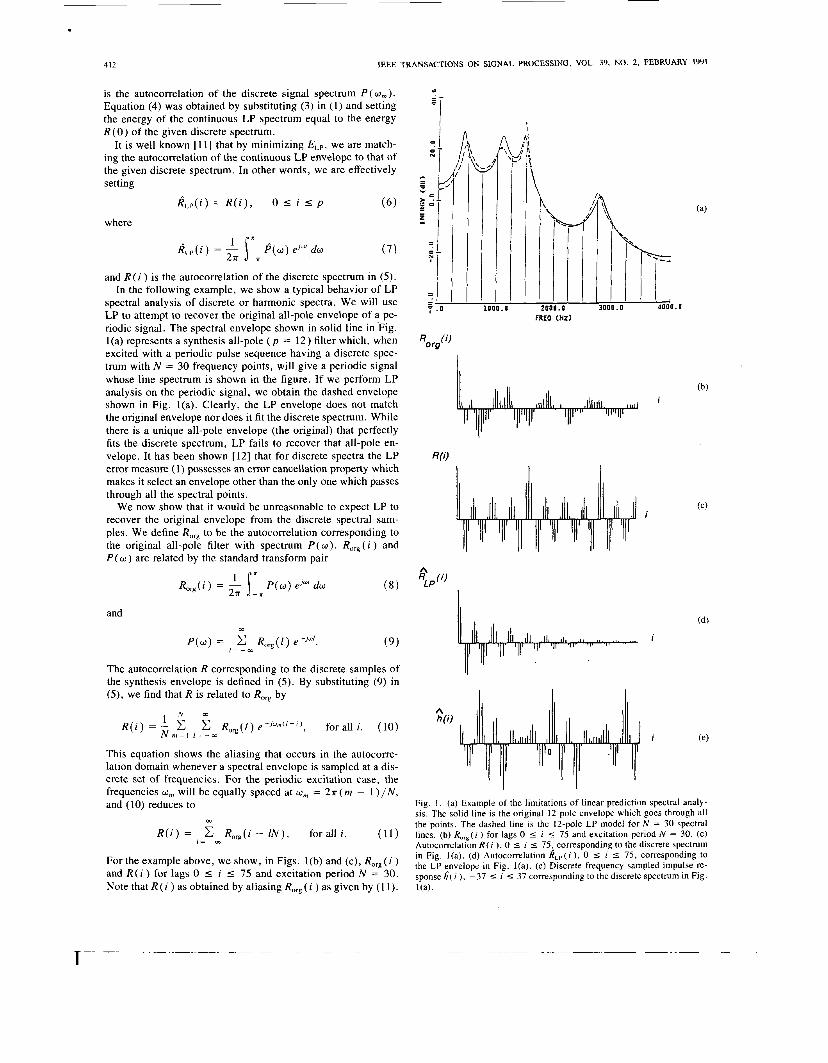
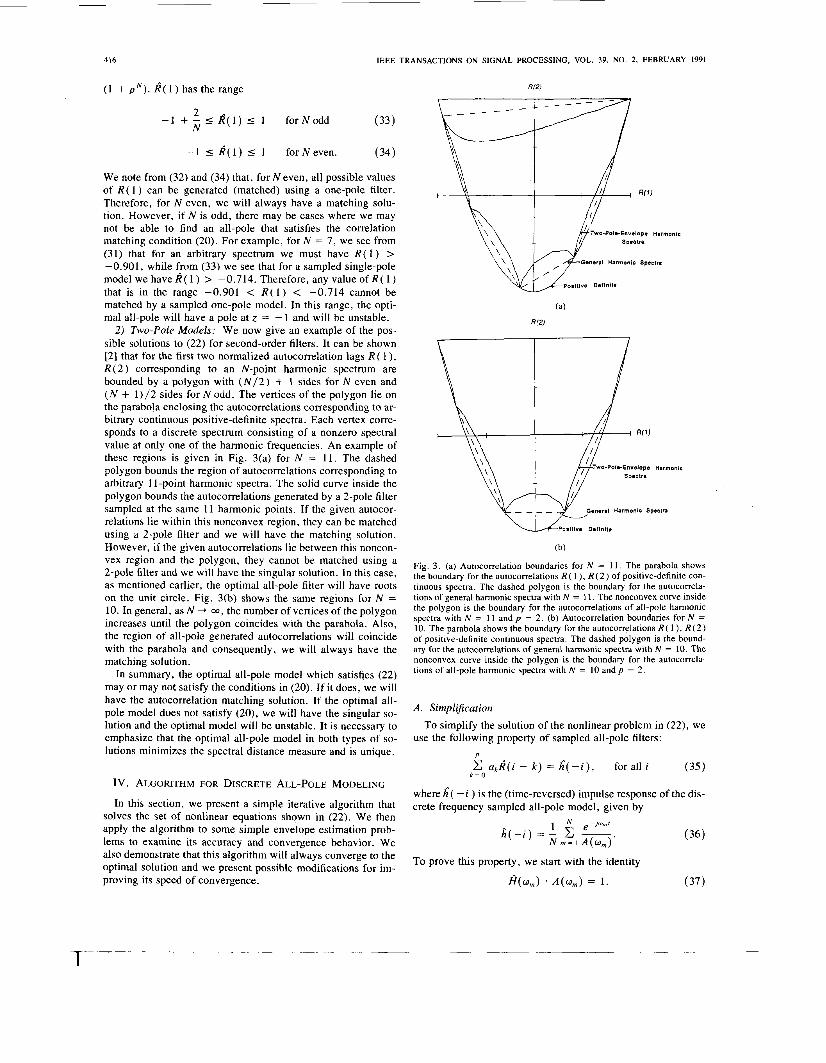
2 ) Two-Pole Models: We now give an example of the possible solutions to (22) for second-order filters. It can be shown [2] that for the first two normalized autocorrelation lags R ( 1 ), R(2) corresponding to an N-point harmonic spectrum are bounded by a polygon with (N/2 ) + 1 sides for N even and ( N + 1)/2 sides for N odd. The vertices of the polygon lie on the parabola enclosing the autocorrelations corresponding to arbitrary continuous positive-definite spectra. Each vertex corresponds to a discrete spectrum consisting of a nonzero spectral value at only one of the harmonic frequencies. An example of these regions is given in Fig. 3(a) for N = 11. The dashed polygon bounds the region of autocorrelations corresponding to arbitrary 1 1-point harmonic spectra. The solid curve inside the polygon bounds the autocorrelations generated by a 2-pole filter sampled at the same 11 harmonic points. If the given autocorrelations lie within this nonconvex region, they can be matched using a 2-pole filter and we will have the matching solution. However, if the given autocorrelations lie between this nonconvex region and the polygon, they cannot be matched using a 2-pole filter and we will have the singular solution. In this case, as mentioned earlier, the optimal all-pole filter will have roots on the unit circle. Fig. 3(b) shows the same regions for N = 10. In general, as N + CO, the number of vertices of the polygon increases until the polygon coincides with the parabola. Also, the region of all-pole generated autocorrelations will coincide with the parabola and consequently, we will always have the matching solution.

In summary, the optimal all-pole model which satisfies (22) may or may not. satisfy the conditions in (20). If it does, we will have the autocorrelation matching solution. If the optimal all- pole model does not satisfy (20), we will have the singular solution and the optimal model will be unstable. It is necessary to emphasize that the optimal all-pole model in both types of solutions minimizes the spectral distance measure and is unique.

Iv. ALGORITHM FOR DISCRETE ALL-POLE MODELING

In this section, we present a simple iterative algorithm that solves the set of nonlinear equations shown in (22). We then apply the algorithm to some simple envelope estimation problems to examine its accuracy and convergence behavior. We also demonstrate that this algorithm will always converge to the optimal solution and we present possible modifications for im- proving its speed of convergence.

_ _ _ - - - L F T

c-

U P o s i t i v a Definite

(b)

Fig. 3 . (a) Autocorrelation boundaries for N = 1 1 . The parabola shows the boundary for the autocorrelations R ( 1 ), R ( 2 ) of positive-definite continuous spectra. The dashed polygon is the boundary for the autocorrelations of general harmonic spectra with N = 11. The nonconvex curve inside the polygon is the boundary for the autocorrelations of all-pole harmonic spectra with N = 11 and p = 2. (b) Autocorrelation boundaries for N = IO. The parabola shows the boundary for the autocorrelations R ( 1 ), R ( 2 ) of positive-definite continuous spectra. The dashed polygon is the boundary for the autocorrelations of general harmonic spectra with N = 10. The nonconvex curve inside the polygon is the boundary for the autocorrelations of all-pole harmonic spectra with N = 10 and p = 2.

A. Sirnplijication

use the following property of sampled all-pole filters: To simplify the solution of the nonlinear problem in (22), we

P

C akk( i - k ) = k ( - i ) , for all i (35) k = O

where h^( - i ) is the (time-reversed) impulse response of the discrete frequency sampled all-pole model, given by

To prove this property, we start with the identity

(37) &(U,) A(Um) = 1.

I


Multiplying the H*(a,), and substituting (2), we get

p(w,) * A ( w , ) = f i*(w,).

C ukP(um) e-jwfnk = A*(o,).

(38)

By expanding A ( a,), we have P

(39) k = O

Multiplying both sides by eJwmr, averaging over U , E a, and using the definition of 8( i ) in (21), we obtain

D . N

for all i .

By substituting the all-pole property (35) into the minimization condition (22), we obtain the following set of equations relating the all-pole predictor coefficients to the given autocorrelation sequence:

P c U $ ( i - k ) = &( - j ) , 0 I i 5 p . (41) k = O

The equations in (41) are written in vector form as

Ra = h (42 1 where h is a column vector with elements 6( - i ), 0 s i s p . For the continuous spectrum case, we have &( i ) = 0 for i < 0 (or h( - i ) = 0 for i > 0) and this set of equations reduces to that of-regular linear prediction in (3) and (4). In fact, LP assumes h ( i ) = 0 for i < 0 for both discrete and continuous spectra. However, for the discrete spectrum case, h ( - i ) is nonzero in general. For the example in Fig. 1, h ( i ) is shown for -37 s i r: 37 in Fig. l(e). It is clear that assuming h ( i ) = 0 for i < 0 is a gross approximation which produces large errors in the LP envelope estimates. In DAP modeling, we are after the exact solution to the set of equations in (41). However, the set in (41) is nonlinear since h( - i ) depends on the values of the all-pole coefficients { uk }. This nonlinear set of equations can be solved iteratively using the algorithm presented below.

417

6) Solve (41) for the new estimate of { a k } .

7) Evaluate E,, using (2) and (14). 8) If the reduction in EIS from previous iterations is greater

than some threshold T, go to step 4; else continue. 9) Normalize the coefficients to satisfy (29).

10) stop. Computationally, the DAP algorithm is more intensive than

LP. Each iteration of the above algorithm requires two real DFT's of size N and the solution of a set of p + 1 linear equations. It is important to note that the autocorrelation matrix R in (41) is constant throughout the iterations, and therefore need only be inverted once. Also, R is Toeplitz symmetric, which allows the use of efficient algorithms in the solution of (41).

C. Examples

To demonstrate that the DAP theory and the algorithm given above are basically sound, we applied the algorithm to the harmonic discrete spectrum in Fig. l(a) and the nonharmonic discrete spectrum in Fig. 2(a). As expected, in both cases DAP was able to recover the original all-pole filter, with the resulting spectrum in each case being almost identical to the original (solid) envelope shown in the figures.

In Section V, we present and discuss the results of applying DAP to real and synthetic speech. But first, we present the convergence properties of the DAP algorithm.

D. Algorithm Convergence

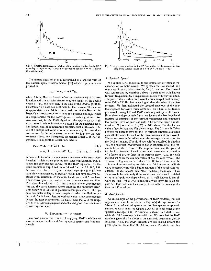
To examine the convergence characteristics of the DAP algorithm, we show in Fig. 4 plots of the spectral error EdB as a function of the iteration number for discrete spectra obtained from the 12-pole example of Fig. 1. The lower line shows the behavior of EdB for a spectral sampling of N = 60 while the upper curve corresponds to a sampling of N = 34. By comparing the two curves, we notice that the algorithm converges faster for a higher value of N , partly because the initial LP estimate is closer to the final DAP result. For smaller values of N close to 2p, as shown by the upper curve, we notice that the error decreases every two iterations instead of every iteration. The reason for this behavior will become evident when we analyze the convergence properties of the algorithm.

While the algorithm is intuitive and straightforward and was derived without rigorous mathematics, we will show that it is fundamentally sound and its behavior is not at all surprising. We will use the vector notation introduced earlier to prove that the algorithm is equivalent to a well-known fast gradient technique and suggest an improvement to the algorithm which increases convergence speed.

The algorithm in Section IV-B can be given in vector notation as follows. Given an estimate a, of the vector a at iteration m, we compute the vector h,. Then, the new estimate a, + , is given from (42) as

B. m e Algorithm

The algofithm used for determining the predictors ak is straightforward; it involves two steps repeated iteratively:

Given an estimate of the predictor, evaluate &( - i using

Given the new estimate of &(

The algorithm in detail is as follows.

(36). ), solve the now

equations (41) for a new estimate of the predictors.

1) Perform peak picking on the spectrum of the speech signal. Obtain the locations w,, the magnitudes P(w,), and the number N of the peaks. (Note that the peak frequencies do not U,+, = ~ - I i i , = R-IR m a m. (43)

With simple manipulation of the above equation, we obtain have to be intege; multiples of some fundamental pitch. How- ever, to minimize the number of spurious peaks, one could apply quasi-harmonic constraints when dealing with voiced speech U,,, = U, - R - ~ ( R - R,)u,. (44) t141.1

from ( 5 ) .

But we see from the derivation of (23) that 2) Given w, and P( U,) for 1 I rn I N , compute R( i )

g, = 2(R - Rm)am (45 1 3) Using ordinary linear prediction, find an initial estimate

4) Compute A ( u , ) for 1 I m I N . is the gradient g at iteration m. Therefore, the update equation in (44) reduces to

of ( a k } , 0 I k I p .

5) Evaluate h( - i ) , 0 5 i I p , using (36). % + I = a, - (2R)-'g",. (46)


040 ' 0 I? lR

Fig. 4. Spectral error E,,, as a function of the iteration number for the DAP modeling example in Fig. l(a) and for excitation periods N = 34 (top) and N = 60 (bottom).

The update equation (46) is recognized as a special form of the classical quasi-Newton method [ 101 which in general is expressed as

a,,, = a, - as-lg,

where S is the Hessian (matrix of second derivatives) of the cost function and a! is a scalar determining the length of the update vector S-lg,. We note that, in the case of the DAP algorithm, the 2R matrix is used as an estimate for the Hessian. This choice is appropriate since 2R is a good estimate of the Hessian for large N (it is exact for N --t 03 ) and it is positive definite, which is a requirement for the convergence of such algorithms. We also note that, for the DAP algorithm, the update scalar is always set to l . While this value is optimal for the quadratic case, it is suboptimal for nonquadratic problems such as this one. The use of a suboptimal value of a! is the reason why the error does not necessarily decrease every iteration. To improve the convergence speed, we incorporate an update scalar a! in our algorithm. The algorithm is then modified to

U,+l = a, - Q!(2R)-lgm (47)

= a,(l - a! ) + a!R-'h^,, 0 5 Q! I 1 . (48)

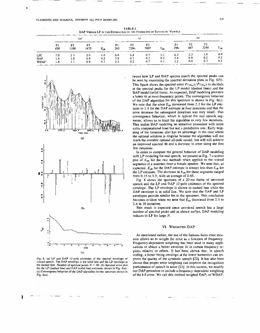
A proper choice of a! can guarantee a decrease in the error every iteration, which would provide for faster convergence. Fig. 5 shows the convergence curves for the DAP algorithm for the same example in Fig. 4 with N = 34 and for a! = 0.1, 0.5, 1 .O. We note that, for Q! = 1 (the standard algorithm in (43)), we have slow convergence. Moreover, we do not have an error decrease every iteration. On the other hand, for a! = 0.5, we have a fast convergence rate and an error decrease every iteration. The algorithm with a! = 0.: has a much slower convergence rate and the curve flattens before attaining the minimum error. This behavior is typical of gradient techniques where if the update parameter is larger than its optimal value, oscillations occur and if it is lower than its optimal value, slow convergence occurs. In most experiments, we have found that cx in the range 0.4 I a! I 0.8 was adequate and achieved good results in terms of convergence speed.

V. EXPERIMENTAL RESULTS We now present the results of applying DAP modeling to

short-term spectra obtained from synthetic speech and from real speech.

a 4

:?U

Fig. 5 . E,, versus iteration for the DAP algorithm for the example in Fig. l(a) using various values of a with N = 34 andp = 12.

A . Synthetic Speech

We applied DAP modeling to the estimation of formant frequencies of synthetic vowels. We synthesized one-second long segments of each of three vowels, led, lit, and lul. Each vowel was synthesized by exciting a fixed 12-pole filter with known formant frequencies by a sequence of pulses with varying pitch. The pitch values within each vowel were changed continuously from 100 to 350 Hz, but never higher than the value of the first formant. We then estimated the spectral envelope of the synthetic speech for every frame of 20 ms (for a total of 50 frames per vowel) using LP and DAP modeling with p = 12 poles. From the envelope in each frame, we located the first three local maxima as estimates of the formant frequencies and computed the percent error ofieach estimate. The percent error was defined as I % I = ( I F - { I / F ) x 100 where F is the known value of the formant and F is the estimate. The first row in Table 1 shows the percent error for the LP formant estimates averaged over all 50 frames for each of the three formants of each vowel. The second row in the table shows the average percent error for the DAP estimates. (The third row will be described in Section VI). We note that DAP produced better estimates of all the formants for all three vowels. The improvement was the greatest for the first formant of each vowel and constituted a reduction of a factor of two to three in the percent error. Also, for each method we show the average value of E,, for each vowel. The decrease in EdB was on the order of 1 (dB) for all three vowels.

It would be misleading to claim that DAP modeling will always necessarily provide a better estimate of the vocal tract res- onances for real speech than other modeling techniques. This claim would be valid only if the vocal tract can be well modeled using an all-pole envelope which, as is well known is not always the case. What DAP modeling always provides is an all- pole envelope that is on the average closer to the harmonic peaks than the LP envelope.

B. Real Speech

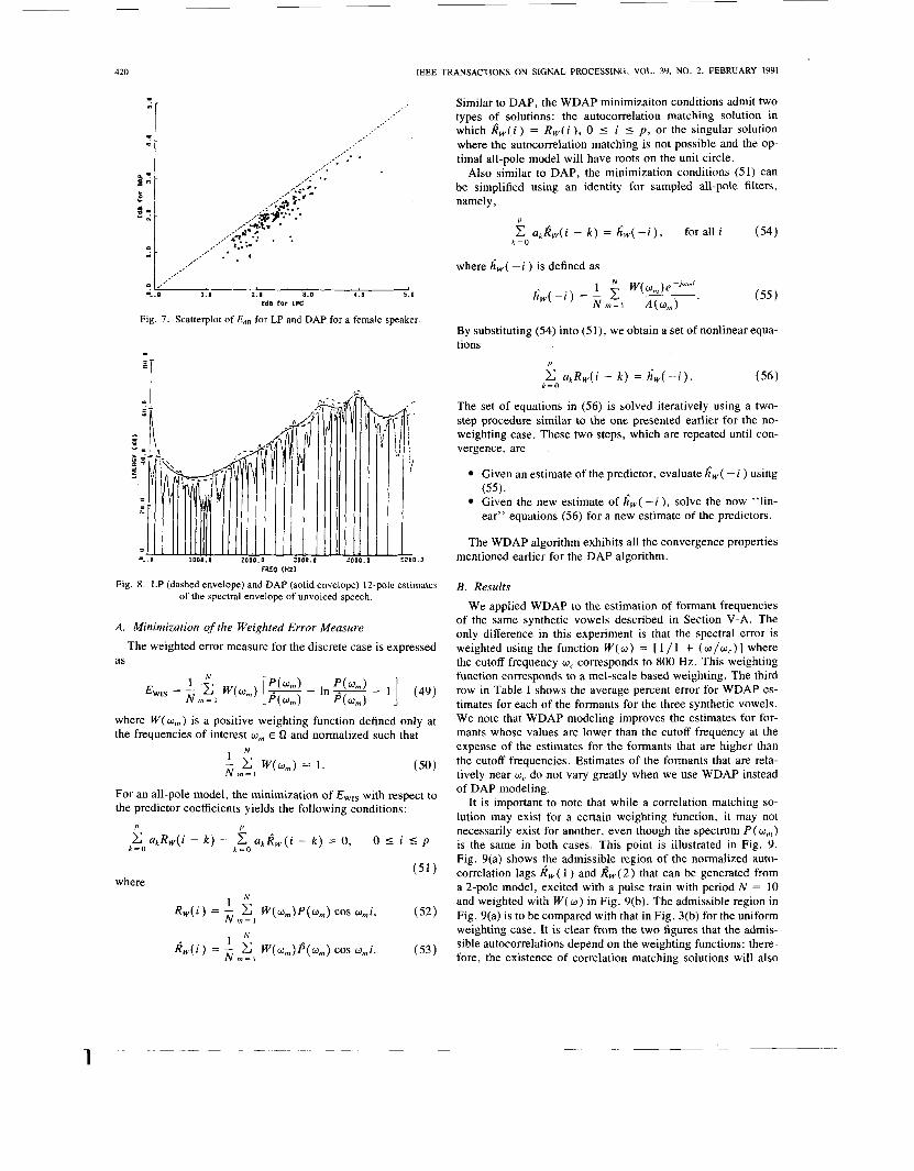
As an example of the performance of DAP modeling on real segments of speech, we show in Fig. 6(a) the spectrum of a 20-ms frame of voiced speech and its line spectrum approximation. We also show the LP and DAP 12-pole estimates of the spectral envelope. The LP estimate is shown as a dashed line while the DAP envelope is the solid line. We note that the DAP envelope generally fits closer to the harmonic peaks than the LP envelope. Also, the DAP formants are less biased toward the given spectral peaks than the LP formants. The difference be-

I


TABLE I DAP VERSUS LP IN THE ESTIMATION OF THE FORMANTS OF SYNTHETIC VOWELS

/er/ til lul

F1 F2 F3 F1 F2 F3 F1 F2 F3 430 1100 1475 E,, 265 2296 3007 E,, 296 867 2240 Em

6 .6 0.8 0.7 1 . 1 6.3 2 .3 1 .o 0.9 7.0 2.3 2.6 1 .o LPC DAP WDAP ' 1.8 1 . 1 0 .9 0.1

1.8 1.0 0.9 0.2 3.0 0.1 0.2 0.3 2.4 0.8 0.2 0.2 2.3 0 .2 0.7 0.1 2.2 0.8 0.3 0.1

- A I

- 0 1 2 3 4 5 6 7 (1 9 10 ITER

(C)

Fig. 6. (a) LP and DAP 12-pole estimates of the spectral envelope of voiced speech. The DAP envelope is the solid line and the LP envelope is the dashed line. Number of spectral points N = 40. (b) Spectral e m r plot for the LP (dashed line) and DAP (solid line) estimates shown in Fig. 6(a). (c) Convergence behavior of the DAP algorithm for the spectrum shown in Fig. 6(a).

tween how LP and DAP spectra match the spectral peaks can be seen by examining the spectral deviation plots in Fig. 6(b). This figure shows the spectral error P(o,)/~(w,) in decibels at the spectral peaks for the LP model (dashed lines) and the DAP model (solid lines). As expected, DAP modeling provides a better fit at most frequency points. The convergence behavior of the DAP algorithm for this spectrum is shown in Fig. 6(c). We note that the error EdB decreased from 2.2 for the LP estimate to 1.4 for the DAP estimate in four iterations and that the error decrease for subsequent iterations was very small. This convergence behavior, which is typical for real speech segments, allows us to limit the algorithm to very few iterations. This makes DAP modeling an attractive procedure with some extra computational load but not a prohibitive one. Early stop- ping of the iterations also has an advantage in the case where the optimal solution is singular because the algorithm will not reach the unstable optimal all-pole model, but will still achieve an improved spectral fit and a decrease in error using the first few iterations.

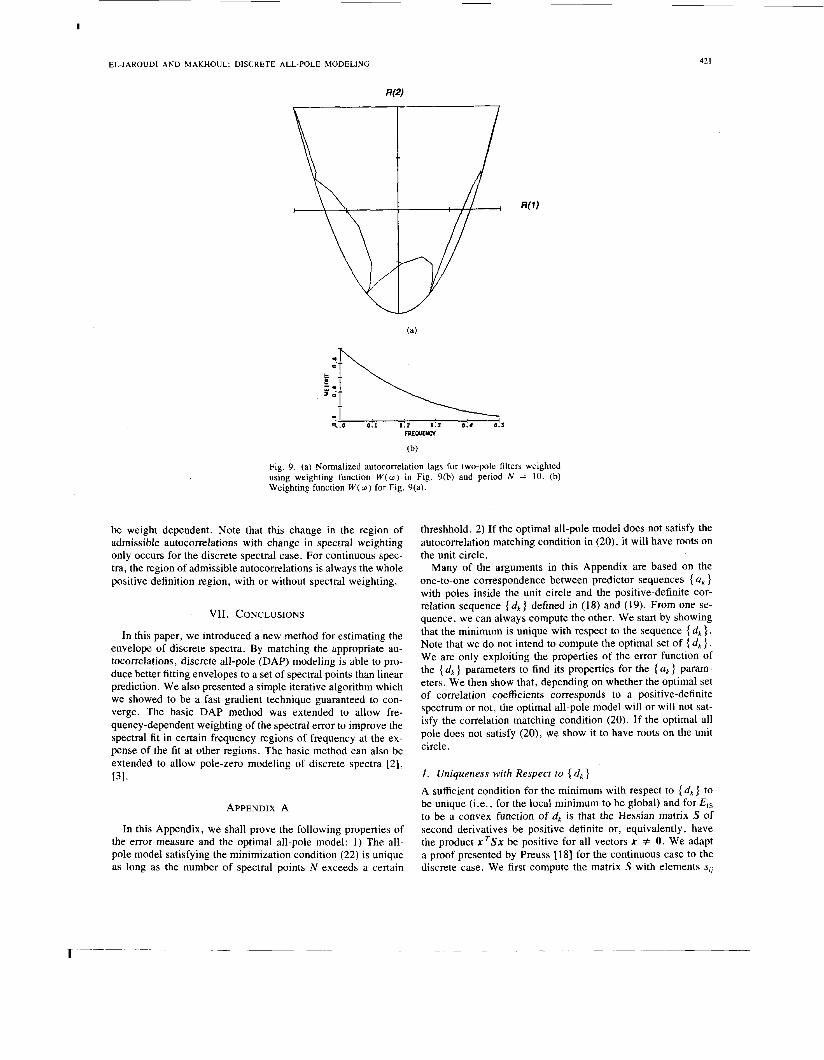
In order to compare the general behavior of DAP modeling with LP modeling for real speech, we present in Fig. 7 a scatter plot of E d , for the two methods when applied to the voiced segments of a sentence from a female speaker. We note that, as expected, EdB for the DAP estimate is always less than E d B for the LP estimate. The decrease in for these segments ranged from 0.15 to 3.5, with an average of 0.65.

Fig. 8 shows the spectrum of a 20-111s frame of unvoiced speech and the LP and DAP 12-pole estimates of the spectral envelope. The LP envelope is shown in dashed line while the DAP envelope is in solid line. We note that the DAP and LP envelopes provide similar fits to the spectrum. This conclusion becomes evident when we note that E, jB decreased from 2.5 to 2.4 in 10 iterations.

This result is expected since unvoiced speech has a large number of spectral peaks and as shown earlier, DAP modeling reduces to LP for large N .

VI. WEIGHTED DAP

As mentioned earlier, the use of the Itakura-Saito error measure allows us to weight the error as a function of frequency. Frequency-dependent weighting has been used in many applications to obtain a better envelope fit in certain frequency regions relative to others. It has been shown that, in speech coding, a better fitting envelope at the lower harmonics can improve the quality of the synthetic speech [22]. It has also been shown that proper error weighting can improve the recognition performance of speech in noise [ZI]. In this section, we modify our DAP procedure to include a frequency-dependent weighting of the I-S error. We call this method weighed DAP, or WDAP.


9. D 1.0 2 .0 3 . 0 9.0 5 .0 Ed8 for LFC

Fig. 7 . Scatterplot of E,, for LP and DAP for a female speaker.

=. . U 1000.0 2000.0 :ooo.o :ooo.o EJUO.9 w o (HZ)

Fig. 8. LP (dashed envelope) and DAP (solid envelope) 12-pole estimates of the spectral envelope of unvoiced speech.

A. Minimization of the Weighted Error Measure

as The weighted error measure for the discrete case is expressed

where W ( U , ) is a positive weighting function defined only at the frequencies of interest U,,, E Q and normalized such that

I N - c W ( U , ) = 1. (50 ) N m = 1

For an all-pole model, the minimization of Ewls with respect to the predictor coefficients yields the following conditions:

P P

k = O k = O C akR,( i - k ) - C akk,(i - k ) = 0, o 5 i 5 p

(51)

( 5 2 )

(53)

where

l N

I N

R , ( i ) = - c W(o,)P(o,) cos ami, N m = l

R , ( i ) = - N m = \ C ~ ( w , , ~ ) P ( w , ) cos w,i.

Similar to DAP, the WDAP minimizaiton conditions admit two types of solutions: the autocorrelation matching solution in which R , ( i ) = R w ( i ) , 0 5 i I p , or the singular solution where the autocorrelation matching is not possible and the optimal all-pole model will have roots on the unit circle.

Also similar to DAP, the minimization conditions (51) can be simplified using an identity for sampled all-pole filters, namely,

P

C akRw(i - k ) = & ( - i ) , for all i (54) k = O

where h,( - i ) is defined as

( 5 5 )

By substituting (54) into (51), we obtain a set of nonlinear equations

The set of equations in (56) is solved iteratively using a two- step procedure similar to the one presented earlier for the no- weighting case. These two steps, which are repeated until convergence, are

Given an estimate of the predictor, evaluate k,( - i ) using

Given the new estimate of 6,( - i ), solve the now "linear" equations (56) for a new estimate of the predictors.

The WDAP algorithm exhibits all the convergence properties

(55) .

mentioned earlier for the DAP algorithm.

B. Results

We applied WDAP to the estimation of formant frequencies of the same synthetic vowels described in Section V-A. The only difference in this experiment is that the spectral error is weighted using the function W ( U ) = [ 1 / 1 + ( U / a c ) ] where the cutoff frequency U , corresponds to 800 Hz. This weighting function corresponds to a mel-scale based weighting. The third row in Table I shows the average percent error for WDAP estimates for each of the formants for the three synthetic vowels. We note that WDAP modeling improves the estimates for formants whose values are lower than the cutoff frequency at the expense of the estimates for the formants that are higher than the cutoff frequencies. Estimates of the formants that are rela- tively near U , do not vary greatly when we use WDAP instead of DAP modeling.

It is important to note that while a correlation matching solution may exist for a certain weighting function, it may not necessarily exist for another, even though the spectrum P ( U , )

is the same in both cases. This point is illustrated in Fig. 9. Fig. 9(a) shows the admissible region of the normalized autocorrelation lags R,( 1 ) and &,( 2 ) that can be generated from a 2-pole model, excited with a pulse train with period N = 10 and weighted with W ( U ) in Fig. 9(b). The admissible region in Fig. 9(a) is to be compared with that in Fig. 3(b) for the uniform weighting case. It is clear from the two figures that the admissible autocorrelations depend on the weighting functions: therefore, the existence of correlation matching solutions will also

I


R(2)

42 I

(b)

Fig. 9 . (a) Normalized autocorrelation lags for two-pole filters weighted using weighting function W ( w ) in Fig. 9(b) and period N = 10. (b) Weighting function W ( w ) for Fig. 9(a).

be weight dependent. Note that this change in the region of admissible autocorrelations with change in spectral weighting only occurs for the discrete spectral case. For continuous spectra, the region of admissible autocorrelations is always the whole positive definition region, with or without spectral weighting.

VII. CONCLUSIONS

In this paper, we introduced a new method for estimating the envelope of discrete spectra. By matching the appropriate autocorrelations, discrete all-pole (DAP) modeling is able to produce better fitting envelopes to a set of spectral points than linear prediction. We also presented a simple iterative algorithm which we showed to be a fast gradient technique guaranteed to converge. The basic DAP method was extended to allow frequency-dependent weighting of the spectral error to improve the spectral fit in certain frequency regions of frequency at the expense of the fit at other regions. The basic method can also be extended to allow pole-zero modeling of discrete spectra [2], [31.

APPENDIX A

In this Appendix, we shall prove the following properties of the error measure and the optimal all-pole model: 1 ) The all- pole model satisfying the minimization condition (22) is unique as long as the number of spectral points N exceeds a certain

threshhold. 2) If the optimal all-pole model does not satisfy the autocorrelation matching condition in (20), it will have roots on the unit circle.

Many of the arguments in this Appendix are based on the one-to-one correspondence between predictor sequences { ak 1 with poles inside the unit circle and the positive-definite correlation sequence { d k } defined in (18) and (19). From one sequence, we can always compute the other. We start by showing that the minimum is unique with respect to the sequence { dk } . Note that we do not intend to compute the optimal set of { dk } . We are only exploiting the properties of the error function of the { dk } parameters to find its properties for the { uk 1 parameters. We then show that, depending on whether the optimal set of correlation coefficients corresponds to a positive-definite spectrum or not, the optimal all-pole model will or will not satisfy the correlation matching condition (20). If the optimal all pole does not satisfy (20), we show it to have roots on the unit circle.

1. Uniqueness with Respect to { dk } A sufficient condition for the minimum with respect to { dk 1 to be unique (i.e., for the local minimum to be global) and for EIS to be a convex function of dk is that the Hessian matrix S of second derivatives be positive definite or, equivalently, have the product x T S x be positive for all vectors x # 0. We adapt a proof presented by Preuss [ 181 for the continuous case to the discrete case. We first compute the matrix S with elements s,,


= d 2 E I s / a d j a d j , 0 I i, j I p. Using the definition of p(o) in (17), one can show that

a2EIS 1 s.. = - = - C B 2 ( w , ) cos iw, cos jam (A.I) ‘’ adiadj N m = I

and P P

. N D D I

= - c ~*(w,) ,2 ,k xjxi cos jw, cos iw,. N m = 1 j = o r = O

Since the summations over i and j are separable, we can write

(‘4.3)

For the Hessian to be positive definite, we need to have at least one term inside the summation be different from zero for all x # 0. In other words, we need

I)

C xi cos w,i # 0, i = O

for x # 0 for at least one frequency point w, E 0. (A.4)

This condition can be written in vector notation as

Cx # 0, forx # 0 (A.5)

where C is an N X ( p + 1 ) matrix with cos w, i being the entry of the mth row and the ith column. Since x # 0, the condition in (A.5) is satisfied if the matrix is of rank r >- p + 1. The rank or number of linearly independent rows of this matrix equals the number of distinct frequency points. It is important to note that w and -w do not qualify as distinct frequencies since they produce identical rows in the matrix. Therefore, r >- p + 1 can be written as

p + 1 5 No,u.

where Nosu is the number of frequency points in the range [0, XI. This inequality translates into the following conditions depending on what the set Q of discrete frequencies includes:

N 2

N - 1 P I - 2

N 2

p I - i f O E Q a n d n E Q (‘4.7)

if either 0 E Q or ?r E Q (A.8)

p s - - 1 otherwise. (A.9)

It is these conditions that guarantee at least one of the terms in the summation in (A.3) to be different from zero, and therefore, the uniqueness condition to be satisfied.

In conclusion, the error is convex in { d k } and therefore the optimal set { d k } is unique if the condition in (A.6) is satisfied.

Note that (A.6) gives the minimum number of spectral points required for uniqueness for a given model order.

The form of the optimal all-pole model will depend on whether the unique optimal value of { dk} occurs within the region corresponding to positive definite spectra or outside it. Below we consider both possibilities and derive the properties of the optimal all-pole predictors { a k } based on those derived above for the set { d , } .

2. Autocorrelation Matching Solution

If the optimal set of { dk 3 corresponds to a positive-definite spectrum, then the corresponding { a k } sequence will exist and will have poles inside the unit circle. In this case, the optimal all-pole model will satisfy the matching condition (20) and the minimization condition (22) (hence the name matching solution). Moreover, since the optimal sequence { dk } is unique (as shown by (A.3) above), the corresponding minimum-phase all- pole madel { a k } will also be unique. In terms of tke matrix equation (23), this solution makes the matrix ( R - R ) identi- cally zero and, therefore, (23) will be satisfied by the corresponding all-pole model.

3. Singular Solution

For the case where the unique local minimum in { dk } is non- positive-definite, there will be no local minimum among positive definite spectral models. However, given the convexity of the error in { dk } , the optimal positive-definite { dk } sequence (the one which produces the smallest error among positive-definite spectral models) will be on the boundary of the positive- definite space. Therefore, the corresponding { a k } will also be on the boundary of positive-definite space. In other words, the optimal all-pole will have roots on the unit circle. In terms of the matrix equation (23), the optimal all-pole model is the vector a that corresponds to the zero eigenvalue of the matrix (R - 8 ) .

REFERENCES

B. S. Atal and M . R. Schroeder, “Recent advances in predictive coding-applications to speech synthesis,” in Proc. Speech Com- mun. symp. 1974, pp. 27-31. A. El-Jaroudi, “Discrete spectral modeling with application to speech analysis,” Ph.D. dissertation, Northeastern University, Aug. 1988. A. El-Jaroudi and J . Makhoul, “Discrete pole-zero modeling and applications,” in Proc. IEEE Int. Conf Acoust., Speech, Signal Processing (Glasgow, Scotland), May 1989, pp. 2162-2165. H. Hermansky, “Analysis and synthesis of speech based on spectral transform linear predictive method,” in Proc. IEEE In?. Conf Acoust., Speech, Signal Processing, 1983, pp. 777-780. H. Hermansky, “Spectral envelope sampling and interpolation in linear predictive analysis of speech,” in Proc. IEEE Int. ConJ Acoust. , Speech, Signal Processing, 1984, pp. 2 .2 .1-2.2.4. F. Itakura and S. Saito, “Analysis synthesis telephony based on the maximum likelihood method,” in Proc. 6th Int. Congr. Acoust. (Tokyo, Japan), 1968, pp. C17-C20. F. Itakura and S . Saito, “A statistical method for estimation of speech spectral density and formant frequencies,” Electron. Comrnun. Japan, vol. 53-A, 1970, pp. 36-43. V. Jain and R. Hangartner, “Efficient algorithm for multipulse LPC analysis of speech,” in Proc. IEEE Int. Con5 Acoust., Speech, Signal Processing, 1984, pp. 1.4.1- I .4 .4 . C. Lee, “Robust linear prediction for speech analysis,” in Proc. IEEE Int. Conf Acoust., Speech, Signal Processing, Apr. 1987, pp. 289-292.

I


Luenberger, Linear and Nonlinear Programming. Reading, MA: Addison-Wesley, 1965. J. Makhoul, “Linear prediction: A tutorial review,” Proc. IEEE, vol. 63, no. 4 , pp. 561-580, Apr. 1975. J. Makhoul, “Spectral linear prediction: Properties and applications,” ZEEE Trans. Acoust., Speech, Signal Processing, vol. ASSP-23, no. 3, pp. 283-246, June 1975. J . D Markel and A. H. Gray, Jr., Linear Prediction ofSpeech. New York: Springer, 1976. R. J. McAulay, “Maximum likelihood spectral estimation and its application to narrow-band speech coding,” ZEEE Trans. Acoust., Speech, Signal Processing, vol. ASSP-32, no. 2, pp. 243-251, Apr. 1984. R. Mizoguchi, “Speech analysis by selective linear prediction in the time domain,” in Proc. ZEEE Znt. Conf. Acoust., Speech, Signal Processing, vol. 3, pp. 1573-1576, 1982.

[16] Ay Parker, “Low-bit rate spkech enhancement using a new method of multiple impulse excitation,” in Proc. IEEE Int. Conf. Acoust., Speech, Signal Processing, 1984, pp. 1.5.1-1.5.4.

[17] J. Picone, “Joint estimation of the LPC parameters and the multipulse excitation,” Speech Commun., 1986, pp. 253-260.

[18] R. D. Preuss, “Autoregressive spectral estimation in noise with application to speech analysis,” Ph.D. dissertation, Oklahoma State University, Dec. 1983.

[19] R. C. Rose and M. A. Clements, “All-pole speech modeling with a maximally pulse-like residual,” in Proc. ZEEE Znt. Con$ Acousr., Speech, Signal Processing, 1985, pp. 481-484.

[20] S. Singhal and B. Atal, “0ptimizing.LPC filter parameters for multipulse excitation,” in Proc. IEEE Znt. Conf. Acousr., Speech, Signal Processing, 1983, pp. 781-784.

1211 F. K. Soong and M. M. Sondhi, “A frequency-weighted Itakura spectral distortion measure and its application to speech recognition in noise,” in IEEE Trans. Acoust., Speech, Signal Pro- cessing, vol. 36, pp. 41-48, Jan. 1988.

[22] V. Viswanathan, M. Berouti, A. Higgins, and W. Russell, “A harmonic deviations vocoder for improved narrow-band speech transmission,” in IEEE Int. Conf. Acoust., Speech, Signal Pro- cessing (Paris, France), May 1982, pp. 610-613.

ing algorithms.

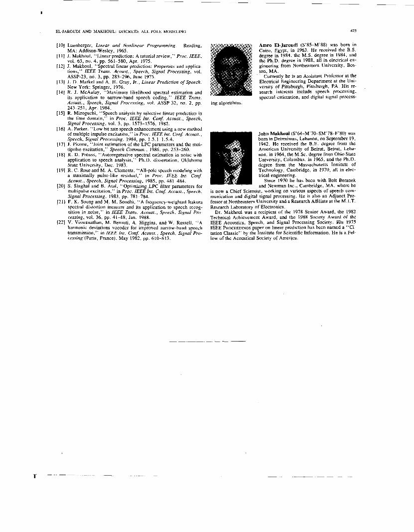
Amro El-Jaroudi (S’85-M’88) was born in Cairo, Egypt, in 1963. He received the B.S. degree in 1984, the M.S. degree in 1984, and the Ph.D. degree in 1988, all in electrical engineering from Northeastern University, Bos- ton, MA.

Currently he is an Assistant Professor at the Electrical Engineering Department at the Uni- versity of Pittsburgh, Pittsburgh, PA. His research interests include speech processing, spectral estimation, and digital signal process-

John Makhoul (S’64-M’70-SM’78-F’80) was born in Deirmimas, Lebanon, on September 19, 1942. He received the B.E. degree from the American University of Beirut, Beirut, Leba- non, in 1964, the M.Sc. degree from Ohio State University, Columbus, in 1965, and the Ph.D. degree from the Massachusetts Institute of Technology, Cambridge, in 1970, all in electrical engineering.

Since 1970 he has been with Bolt Beranek and Newman Inc., Cambridge, MA, where he

is now a Chief Scientist, working on various aspects of speech com- munication and digital signal processing. He is also an Adjunct Pro- fessor at Northeastern University and a Research Affiliate at the M.I.T. Research Laboratory of Electronics.

Dr. Makhoul was a recipient of the 1978 Senior Award, the 1982 Technical Achievement Award, and the 1988 Society Award of the IEEE Acoustics, Speech, and Signal Processing Society. His 1975 IEEE PROCEEDINGS paper on linear prediction has been named a “Ci- tation Classic” by the Institute for Scientific Information. He is a Fel- low of the Acoustical Society of America.

Discrete all-pole modeling - Signal Processing, IEEE Transactions on

Documents