Engineering Genetic Circuits Chris J. Myers Lecture 3: Differential Equation Analysis Chris J. Myers (Lecture 3: ODE Analysis) Engineering Genetic Circuits 1 / 48

Welcome message from author
This document is posted to help you gain knowledge. Please leave a comment to let me know what you think about it! Share it to your friends and learn new things together.
Transcript
Engineering Genetic Circuits
Chris J. Myers
Lecture 3: Differential Equation Analysis
Chris J. Myers (Lecture 3: ODE Analysis) Engineering Genetic Circuits 1 / 48
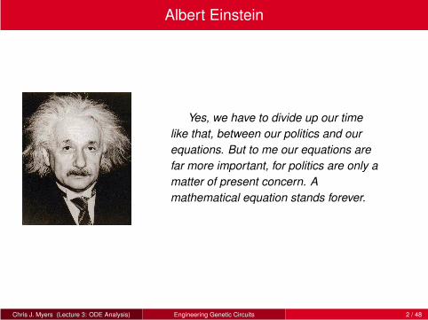
Albert Einstein
Yes, we have to divide up our time
like that, between our politics and our
equations. But to me our equations are
far more important, for politics are only a
matter of present concern. A
mathematical equation stands forever.
Chris J. Myers (Lecture 3: ODE Analysis) Engineering Genetic Circuits 2 / 48
Introduction
Next step of the engineering approach is analysis.
Goal of analysis is to be able to both reproduce experimental results and
make predictions in silico.
Simulation provides unlimited controllability and observability.
Traditional classical chemical kinetics (CCK) utilizes ordinary differential
equations (ODE) to represent system dynamics.
Law of mass action can translate a chemical reaction model into ODEs
known as reaction rate equations.
ODEs typically analyzed using numerical simulation.
Qualitative analysis utilized to understand behavior as initial conditions
and parameter values vary.
Partial differential equations (PDE) utilized when spatial considerations
are important.
Chris J. Myers (Lecture 3: ODE Analysis) Engineering Genetic Circuits 3 / 48

Overview
Classical chemical kinetics
Differential equation simulation
Qualitative ODE analysis
Spatial methods
Chris J. Myers (Lecture 3: ODE Analysis) Engineering Genetic Circuits 4 / 48
A Classical Chemical Kinetic Model
A CCK model tracks concentrations of each chemical species (i.e.,
number of molecules divided by volume, Ω, of cell or compartment).
Assumes reactions occur in a well-stirred volume (i.e., molecules are
equally distributed within the cell) and spatial effects can be neglected.
Assumes reactions occur continuously and deterministically.
Requires that the number of molecules of each species are large.
Chris J. Myers (Lecture 3: ODE Analysis) Engineering Genetic Circuits 5 / 48
A Classical Chemical Kinetic Model (cont)
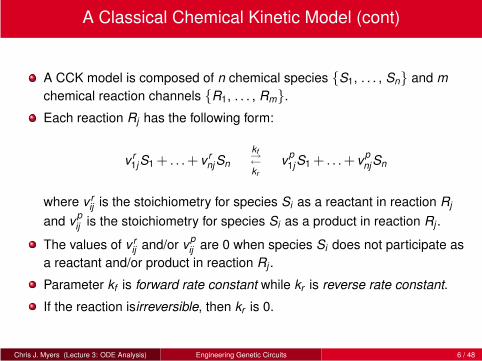
A CCK model is composed of n chemical species S1, . . . , Sn and m
chemical reaction channels R1, . . . , Rm.
Each reaction Rj has the following form:
v r1jS1 + . . .+ v r
njSn
kf→←kr
vp1jS1 + . . .+ v
pnjSn
where v rij is the stoichiometry for species Si as a reactant in reaction Rj
and vpij is the stoichiometry for species Si as a product in reaction Rj .
The values of v rij and/or v
pij are 0 when species Si does not participate as
a reactant and/or product in reaction Rj .
Parameter kf is forward rate constant while kr is reverse rate constant.
If the reaction isirreversible, then kr is 0.
Chris J. Myers (Lecture 3: ODE Analysis) Engineering Genetic Circuits 6 / 48
A Classical Chemical Kinetic Model (cont)
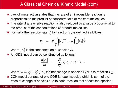
Law of mass action states that the rate of an irreversible reaction is
proportional to the product of concentrations of reactant molecules.
The rate of a reversible reaction is also reduced by a value proportional to
the product of the concentrations of product molecules.
Formally, the reaction rate Vj for reaction Rj is defined as follows:
Vj = kf
n
∏i=1
[Si ]v r
ij − kr
n
∏i=1
[Si ]v
pij
where [Si ] is the concentration of species Si .
An ODE model can be constructed as follows:
d [Si ]
dt=
m
∑j=1
vijVj , 1≤ i ≤ n
where vij = vpij − v r
ij (i.e., the net change in species Si due to reaction Rj ).
CCK model consists of one ODE for each species which is sum of the
rates of change of species due to each reaction that affects the species.
Chris J. Myers (Lecture 3: ODE Analysis) Engineering Genetic Circuits 7 / 48
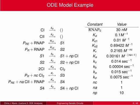
ODE Model Example
CIkd−→ ()
CIIkd−→ ()
PRE +RNAPKo1←→ S1
PR +RNAPKo2←→ S2
S1kb−→ S1+np CI
S2ko−→ S2+np CII
2CIKd←→ CI2
PR +nc CI2Kr←→ S3
PRE +na CII+RNAPKa←→ S4
S4ka−→ S4+np CI
Constant Value
RNAP0 30 nM
Kd 0.1M−1
Ko1 0.01 M−1
Ko2 0.69422 M−1
Kr 0.2165 M−nc
Ka 0.00161 M−(na+1)
ko 0.014 sec−1
kb 0.00004 sec−1
ka 0.015 sec−1
kd 0.0075 sec−1
nc 1
na 1
np 10
Chris J. Myers (Lecture 3: ODE Analysis) Engineering Genetic Circuits 8 / 48

ODE Model Example
d [CI]dt
= np kb[S1]+np ka[S4]−2(Kd [CI]2− [CI2])− kd [CI]
d [CI2]dt
= Kd [CI]2− [CI2]−nc(Kr [PR ][CI2]nc− [S3])
d [CII]dt
= np ko[S2]−na(Ka[PRE ][RNAP][CII]na− [S4])− kd [CII]
d [PR ]dt
= [S2]−Ko2[PR ][RNAP]+ [S3]−Kr [PR ][CI2]nc
d [PRE ]dt
= [S1]−Ko1[PRE ][RNAP]+ [S4]−Ka[PRE ][RNAP][CII]na
d [RNAP]dt
= [S1]−Ko1[PRE ][RNAP]+ [S2]−Ko2[PR ][RNAP]+
[S4]−Ka[PRE ][RNAP][CII]na
d [S1]dt
= Ko1[PRE ][RNAP]− [S1]
d [S2]dt
= Ko2[PR ][RNAP]− [S2]
d [S3]dt
= Kr [PR ][CI2]nc− [S3]
d [S4]dt
= Ka[PRE ][RNAP][CII]na− [S4]
Chris J. Myers (Lecture 3: ODE Analysis) Engineering Genetic Circuits 9 / 48
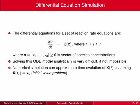
Differential Equation Simulation
The differential equations for a set of reaction rate equations are:
dxi
dt= fi(x), where 1≤ i ≤ n
where x = [x1, . . . ,xn]≥ 0 is vector of species concentrations.
Solving this ODE model analytically is very difficult, if not impossible.
Numerical simulation can approximate time evolution of X(t) assuming
X(t0) = x0 (initial value problem).
Chris J. Myers (Lecture 3: ODE Analysis) Engineering Genetic Circuits 10 / 48
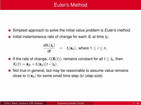
Euler’s Method
Simplest approach to solve the initial value problem is Euler’s method.
Initial instantaneous rate of change for each Si at time t0:
dXi(t0)
dt= fi(x0), where 1≤ i ≤ n.
If the rate of change, fi(X(t)), remains constant for all t ≥ t0, then
Xi(t) = x0i + fi(x0)(t− t0).
Not true in general, but may be reasonable to assume value remains
close to fi(x0) for some small time step ∆t (step size).
Chris J. Myers (Lecture 3: ODE Analysis) Engineering Genetic Circuits 11 / 48
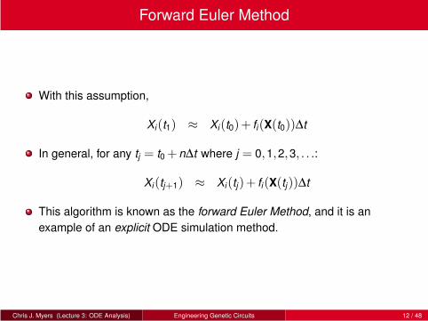
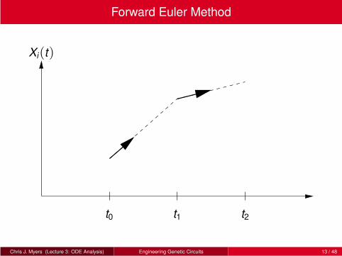
Forward Euler Method
With this assumption,
Xi(t1) ≈ Xi(t0)+ fi(X(t0))∆t
In general, for any tj = t0 +n∆t where j = 0,1,2,3, . . .:
Xi(tj+1) ≈ Xi(tj)+ fi(X(tj))∆t
This algorithm is known as the forward Euler Method, and it is an
example of an explicit ODE simulation method.
Chris J. Myers (Lecture 3: ODE Analysis) Engineering Genetic Circuits 12 / 48
Forward Euler Method
Xi(t)
t0 t1 t2
Chris J. Myers (Lecture 3: ODE Analysis) Engineering Genetic Circuits 13 / 48
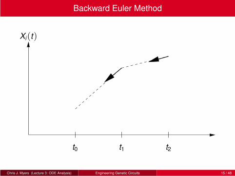
Backward Euler Method
Backward Euler method is an implicit ODE simulation method.
New rate of change cannot be determined directly from current state, but
it must be found implicitly by an equation that must be solved.
Backward Euler method is defined by follows:
Xi(tj+1) ≈ Xi(tj)+ fi(X(tj+1))∆t.
New value of X(tj+1) is determined as the rate at the point that would
have taken you there in a ∆t step.
Since X(tj+1) is not yet known, this equation must be solved using a root
finding technique such as the Newton-Raphson method.
Implicit methods are more complicated, but often more stable for stiff
equations (i.e., those that require a very small time step).
Chris J. Myers (Lecture 3: ODE Analysis) Engineering Genetic Circuits 14 / 48
Backward Euler Method
Xi(t)
t0 t1 t2
Chris J. Myers (Lecture 3: ODE Analysis) Engineering Genetic Circuits 15 / 48
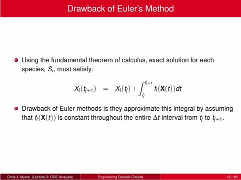
Drawback of Euler’s Method
Using the fundamental theorem of calculus, exact solution for each
species, Si , must satisfy:
Xi(tj+1) = Xi(tj)+Z tj+1
tj
fi(X(t))dt
Drawback of Euler methods is they approximate this integral by assuming
that fi(X(t)) is constant throughout the entire ∆t interval from tj to tj+1.
Chris J. Myers (Lecture 3: ODE Analysis) Engineering Genetic Circuits 16 / 48
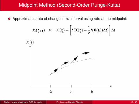
Midpoint Method (Second-Order Runge-Kutta)
Approximates rate of change in ∆t interval using rate at the midpoint:
Xi(tj+1) ≈ Xi(tj)+
[
fi(X(tj)+1
2f (X(tj))∆t)
]
∆t
Xi(t)
t0 t1 t2
Chris J. Myers (Lecture 3: ODE Analysis) Engineering Genetic Circuits 17 / 48
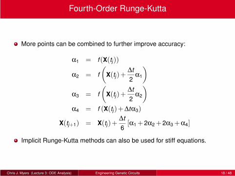
Fourth-Order Runge-Kutta
More points can be combined to further improve accuracy:
α1 = f (X(tj))
α2 = f
(
X(tj)+∆t
2α1
)
α3 = f
(
X(tj)+∆t
2α2
)
α4 = f (X(tj)+∆tα3)
X(tj+1) = X(tj)+∆t
6[α1 +2α2 +2α3 +α4]
Implicit Runge-Kutta methods can also be used for stiff equations.
Chris J. Myers (Lecture 3: ODE Analysis) Engineering Genetic Circuits 18 / 48
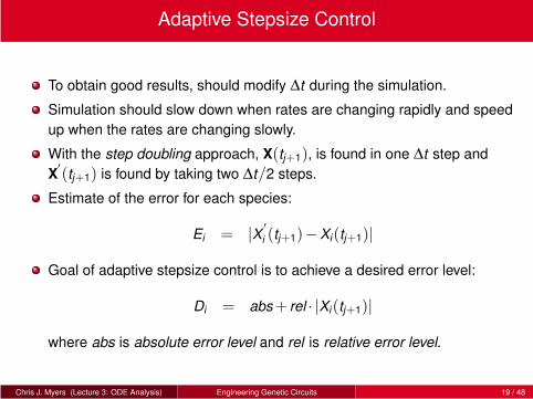
Adaptive Stepsize Control
To obtain good results, should modify ∆t during the simulation.
Simulation should slow down when rates are changing rapidly and speed
up when the rates are changing slowly.
With the step doubling approach, X(tj+1), is found in one ∆t step and
X′(tj+1) is found by taking two ∆t/2 steps.
Estimate of the error for each species:
Ei = |X′
i (tj+1)−Xi(tj+1)|
Goal of adaptive stepsize control is to achieve a desired error level:
Di = abs+ rel · |Xi(tj+1)|
where abs is absolute error level and rel is relative error level.
Chris J. Myers (Lecture 3: ODE Analysis) Engineering Genetic Circuits 19 / 48
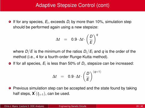
Adaptive Stepsize Control (cont)
If for any species, Ei , exceeds Di by more than 10%, simulation step
should be performed again using a new stepsize:
∆t = 0.9 ·∆t ·
(
D
E
)q
where D/E is the minimum of the ratios Di/Ei and q is the order of the
method (i.e., 4 for a fourth-order Runge-Kutta method).
If for all species, Ei is less than 50% of Di , stepsize can be increased:
∆t = 0.9 ·∆t ·
(
D
E
)(q+1)
Previous simulation step can be accepted and the state found by taking
half steps, X′(tj+1), can be used.
Chris J. Myers (Lecture 3: ODE Analysis) Engineering Genetic Circuits 20 / 48
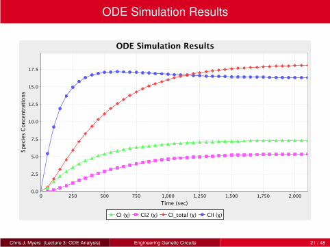
ODE Simulation Results
Chris J. Myers (Lecture 3: ODE Analysis) Engineering Genetic Circuits 21 / 48
Qualitative ODE Analysis
Goal of ODE analysis is to determine properties of the phase space.
Phase space is the set of all possible states of the system.
States are values and current rates of change of each variable.
Numerical simulation only shows one trajectory in the phase space
starting in a given initial condition with specific parameter values.
Goal of qualitative ODE analysis is to determine the complete phase
space based upon any initial condition.
Can also discover how parameter variation affects the phase space.
Chris J. Myers (Lecture 3: ODE Analysis) Engineering Genetic Circuits 22 / 48
One-Dimensional ODE Models
A one-dimensional ODE model with a single parameter, r :
dx
dt= f (x , r)
A state for such a model includes only the value of x and its current rate
of change (or flow) of x , dxdt
.
Can visualize phase space with a graph of x versus dxdt
.
Chris J. Myers (Lecture 3: ODE Analysis) Engineering Genetic Circuits 23 / 48
Saddle-Node Example
dx
dt=−r + x2
Chris J. Myers (Lecture 3: ODE Analysis) Engineering Genetic Circuits 24 / 48
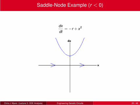
Saddle-Node Example (r < 0)
dx
dt=−r + x2
Chris J. Myers (Lecture 3: ODE Analysis) Engineering Genetic Circuits 25 / 48
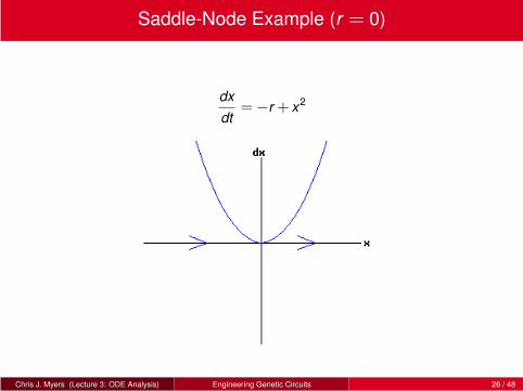
Saddle-Node Example (r = 0)
dx
dt=−r + x2
Chris J. Myers (Lecture 3: ODE Analysis) Engineering Genetic Circuits 26 / 48
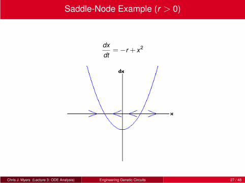
Saddle-Node Example (r > 0)
dx
dt=−r + x2
Chris J. Myers (Lecture 3: ODE Analysis) Engineering Genetic Circuits 27 / 48
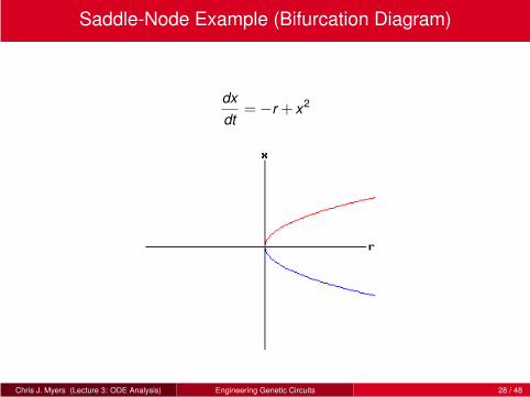
Saddle-Node Example (Bifurcation Diagram)
dx
dt=−r + x2
Chris J. Myers (Lecture 3: ODE Analysis) Engineering Genetic Circuits 28 / 48
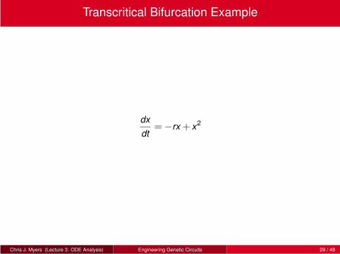
Transcritical Bifurcation Example
dx
dt=−rx + x2
Chris J. Myers (Lecture 3: ODE Analysis) Engineering Genetic Circuits 29 / 48
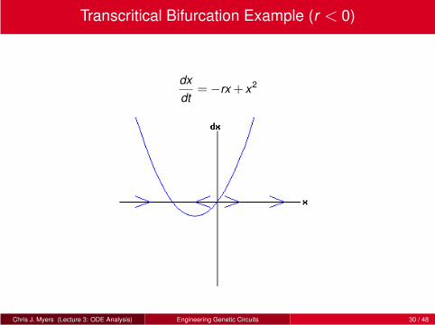
Transcritical Bifurcation Example (r < 0)
dx
dt=−rx + x2
Chris J. Myers (Lecture 3: ODE Analysis) Engineering Genetic Circuits 30 / 48
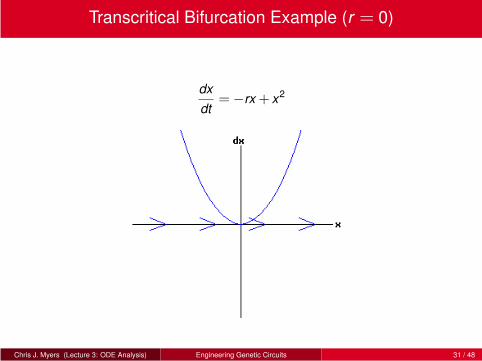
Transcritical Bifurcation Example (r = 0)
dx
dt=−rx + x2
Chris J. Myers (Lecture 3: ODE Analysis) Engineering Genetic Circuits 31 / 48
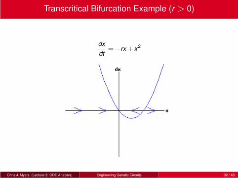
Transcritical Bifurcation Example (r > 0)
dx
dt=−rx + x2
Chris J. Myers (Lecture 3: ODE Analysis) Engineering Genetic Circuits 32 / 48
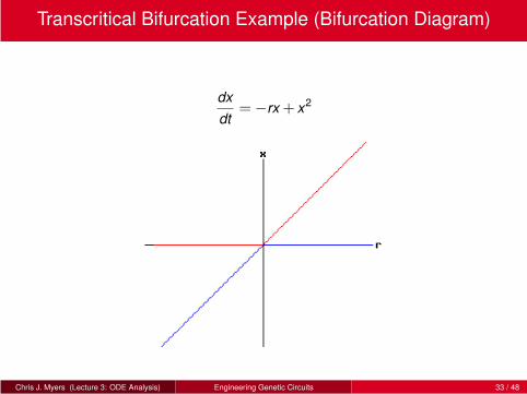
Transcritical Bifurcation Example (Bifurcation Diagram)
dx
dt=−rx + x2
Chris J. Myers (Lecture 3: ODE Analysis) Engineering Genetic Circuits 33 / 48
Pitchfork Bifurcation Example
dx
dt= rx− x3
Chris J. Myers (Lecture 3: ODE Analysis) Engineering Genetic Circuits 34 / 48
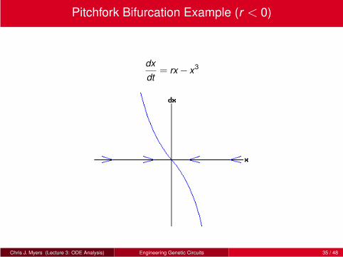
Pitchfork Bifurcation Example (r < 0)
dx
dt= rx− x3
Chris J. Myers (Lecture 3: ODE Analysis) Engineering Genetic Circuits 35 / 48
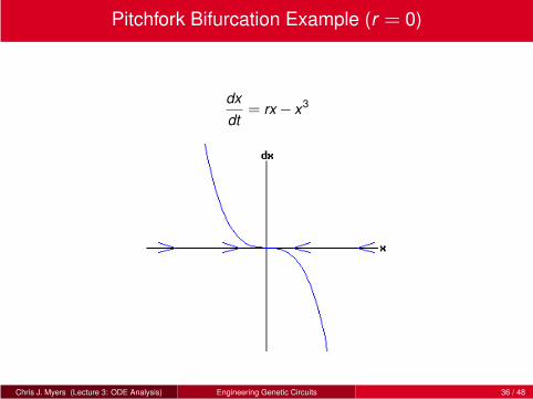
Pitchfork Bifurcation Example (r = 0)
dx
dt= rx− x3
Chris J. Myers (Lecture 3: ODE Analysis) Engineering Genetic Circuits 36 / 48
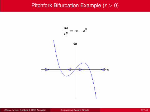
Pitchfork Bifurcation Example (r > 0)
dx
dt= rx− x3
Chris J. Myers (Lecture 3: ODE Analysis) Engineering Genetic Circuits 37 / 48

Pitchfork Bifurcation Example (Bifurcation Diagram)
dx
dt= rx− x3
Chris J. Myers (Lecture 3: ODE Analysis) Engineering Genetic Circuits 38 / 48
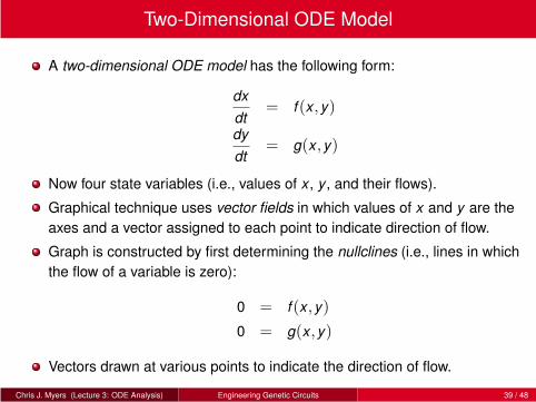
Two-Dimensional ODE Model
A two-dimensional ODE model has the following form:
dx
dt= f (x ,y)
dy
dt= g(x ,y)
Now four state variables (i.e., values of x , y , and their flows).
Graphical technique uses vector fields in which values of x and y are the
axes and a vector assigned to each point to indicate direction of flow.
Graph is constructed by first determining the nullclines (i.e., lines in which
the flow of a variable is zero):
0 = f (x ,y)
0 = g(x ,y)
Vectors drawn at various points to indicate the direction of flow.
Chris J. Myers (Lecture 3: ODE Analysis) Engineering Genetic Circuits 39 / 48
Two-Dimensional ODE Model (cont)
Points in which two nullclines intersect are equilibrium points.
Stability can be determined by looking at the flows in the vicinity of the
equilibrium point.
Qualitative ODE analysis for systems of more than 2 dimensions is
difficult, so one often reduces dimensionality to 2.
Chris J. Myers (Lecture 3: ODE Analysis) Engineering Genetic Circuits 40 / 48
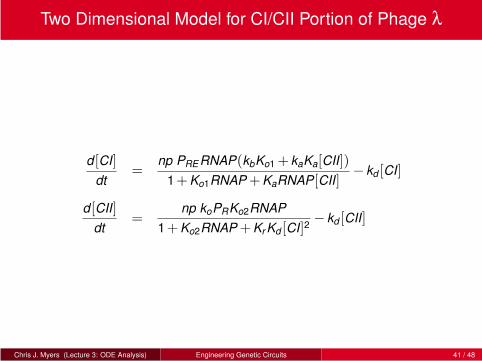
Two Dimensional Model for CI/CII Portion of Phage λ
d [CI]
dt=
np PRERNAP(kbKo1 + kaKa[CII])
1+Ko1RNAP +KaRNAP[CII]− kd [CI]
d [CII]
dt=
np koPRKo2RNAP
1+Ko2RNAP +Kr Kd [CI]2− kd [CII]
Chris J. Myers (Lecture 3: ODE Analysis) Engineering Genetic Circuits 41 / 48
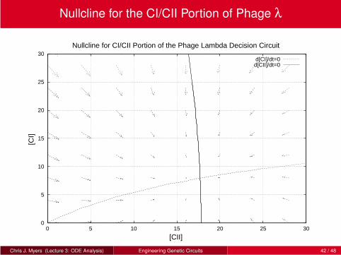
Nullcline for the CI/CII Portion of Phage λ
0
5
10
15
20
25
30
0 5 10 15 20 25 30
[CI]
[CII]
Nullcline for CI/CII Portion of the Phage Lambda Decision Circuit
d[CI]/dt=0 d[CII]/dt=0
Chris J. Myers (Lecture 3: ODE Analysis) Engineering Genetic Circuits 42 / 48
Spatial Methods
ODE models assume spatial homogeneity.
Delays due to diffusion may be important.
Examples:
Diffusion between the nucleus and cytoplasm or other compartments.
Cell differentiation and embryonic development in multicellular organisms
appears to be controlled by gradients of protein concentrations.
Chris J. Myers (Lecture 3: ODE Analysis) Engineering Genetic Circuits 43 / 48
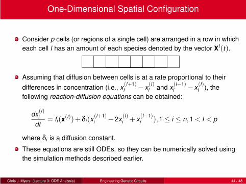
One-Dimensional Spatial Configuration
Consider p cells (or regions of a single cell) are arranged in a row in which
each cell l has an amount of each species denoted by the vector Xl(t).
Assuming that diffusion between cells is at a rate proportional to their
differences in concentration (i.e., x(l+1)i − x
(l)i and x
(l−1)i − x
(l)i ), the
following reaction-diffusion equations can be obtained:
dx(l)i
dt= fi(x
(l))+δi(x(l+1)i −2x
(l)i + x
(l−1)i ),1≤ i ≤ n,1 < l < p
where δi is a diffusion constant.
These equations are still ODEs, so they can be numerically solved using
the simulation methods described earlier.
Chris J. Myers (Lecture 3: ODE Analysis) Engineering Genetic Circuits 44 / 48
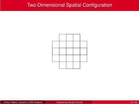
Two-Dimensional Spatial Configuration
Chris J. Myers (Lecture 3: ODE Analysis) Engineering Genetic Circuits 45 / 48
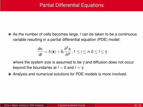
Partial Differential Equations
As the number of cells becomes large, l can be taken to be a continuous
variable resulting in a partial differential equation (PDE) model:
dxi
dt= fi(x)+δi
∂2xi
∂l2,1≤ i ≤ n,0≤ l ≤ γ
where the system size is assumed to be γ and diffusion does not occur
beyond the boundaries at l = 0 and l = γ.
Analysis and numerical solutions for PDE models is more involved.
Chris J. Myers (Lecture 3: ODE Analysis) Engineering Genetic Circuits 46 / 48
More on Spatial Modeling
Reaction-diffusion equations for modeling cell differentiation were
originally proposed by Turing (1951).
Goal of his work is a mathematical model of a growing embryo.
Turing suggested that systems consist of masses of tissues within which
certain substances called morphogens react chemically and diffuse.
Diffusing into a tissue persuades the tissue to develop differently.
The embryo in the spherical blastula stage has spherical symmetry.
Systems with spherical symmetry whose state is changed by chemical
reactions and diffusion remains spherically symmetric.
This cannot result in a non-spherically symmetric organism like a horse.
There are some asymmetries which cause instability and lead to a new
and stable equilibrium without symmetry.
This behavior is very similar to how electrical oscillators get started.
Successfully applied to modeling pattern formation in the Drosophila
embryo (see Kauffman et al. (1978), Bunow et al. (1980), Goodwin and
Kauffman (1990), Lacalli (1990), and Myasnikova et al. (2001)).
Chris J. Myers (Lecture 3: ODE Analysis) Engineering Genetic Circuits 47 / 48
Sources
Differential equation analysis:
Law of mass action - Waage and Guldberg (1864).
Classical chemical kinetics - Wright (2004).
Models of genetic circuits - Goodwin (1963, 1965).
Numerical simulation - Press et al. (1992).
Qualitative ODE analysis - Strogatz (1994).
ODE models:
Phage λ - Reinitz and Vaisnys (1990).
lac operaon - Wong et al. (1997), Vilar et al. (2003), Yildirim and Mackey
(2003), Yildirim et al. (2004), Santillan and Mackey (2004), Hoek and
Hogeweg (2006), etc.
Bacteriophage T7 - Endy et al. (2000), You and Yin (2006), etc.
Trpyptophan synthesis - Giona and Adrover (2002), Xiu et al. (2002),
Santillan and Zeron (2004, 1006), etc.
Circadian rhythms - Leloup and Goldbeter (1998), Ruoff et al. (2001), Ueda
et al. (2001), etc.
The cell cycle - Novak and Tyson (1995), Tyson et al. (1996), Borisuk and
Tyson (1998), Novak et al. (1998), Tyson (1999), Chen et al. (2000), etc.
Chris J. Myers (Lecture 3: ODE Analysis) Engineering Genetic Circuits 48 / 48
Related Documents