Diagnosis and exploration of massively univariate ... - CiteSeerX

Diagnosis and exploration of massively univariate neuroimaging models

Wen-Lin Luo and Thomas E. Nichols*Department of Biostatistics, University of Michigan, Ann Arbor, MI 48109 USA

Received 7 May 2002; revised 13 December 2002; accepted 3 March 2003

Abstract

The goal of this work is to establish the validity of neuroimaging models and inferences through diagnosis and exploratory data analysis.While model diagnosis and exploration are integral parts of any statistical modeling enterprise, these aspects have been mostly neglectedin functional neuroimaging. We present methods that make diagnosis and exploration of neuroimaging data feasible. We use three- andone-dimensional summaries that characterize the model fit and the four-dimensional residuals. The statistical tools are diagnostic summarystatistics with tractable null distributions and the dynamic graphical tools which allow the exploration of multiple summaries in both spatialand temporal/interscan aspects, with the ability to quickly jump to spatiotemporal detail. We apply our methods to a fMRI data set,demonstrating their ability to localize subtle artifacts and to discover systematic experimental variation not captured by the model.© 2003 Elsevier Science (USA). All rights reserved.

Keywords: Diagnosis; Exploratory data analysis; Artifact; Autocorrelation; Global scaling; Interactive visualization

Introduction and motivation

Neuroimaging analyses proceed by localizing brain re-gions exhibiting experimental variation. A PET or fMRIexperiment yields a sequence of large three-dimensionalimages of the subject’s brain, each containing as many as100,000 volume elements or voxels. The typical analysisstrategy is marginal or “massively univariate” (Holmes,1994), where data for each voxel are independently fit withthe same model (Friston et al., 1995). Images of test statis-tics are used to make inference on the presence of an effectat each voxel.

The main purpose of this work is to establish the validityof inferences in neuroimaging through diagnosis of modelassumptions. Hypothesis tests and P values depend on as-sumptions on the data, and inferences should not be trustedunless assumptions are checked. Diagnosis is usually doneby the graphical analysis of residuals (Neter et al., 1996;Draper and Smith, 1998). For example, one standard tool is

a scatter plot of residuals versus fitted values, useful fordiagnosing nonconstant variance, curvature, and outliers.This sort of graphical analysis is not practical since it is notpossible to evaluate 100,000 plots.

The other purpose of this work is to characterize signaland artifacts through exploratory data analysis (EDA;Tukey, 1977). EDA is an important step in any statisticalanalysis, as it familiarizes the analyst with form of theexpected experimental variation, the presence of unex-pected systematic variation, and the character of randomvariation. As with model diagnosis, traditional EDA toolsare graphical and cannot be applied voxel-by-voxel exhaus-tively. Fortunately EDA can also be accomplished by ex-ploring the fit and the residuals (Hoaglin et al., 1983). Amodel partitions data as the sum “Data � Fit � Residuals,”and in neuroimaging data the fit and residuals are individ-ually more amenable to exploration than the full data. Thefit is parameterized by the user and is readily interpretable,while the residuals are homogeneous and unstructured if themodel fits. Interesting features in the residuals can be foundby use of statistics sensitive to structure or inhomogeneity;for example, something as simple as outlier counts per scancan quickly identify interesting scans. Diagnosis and EDAare enmeshed: Diagnosis takes the form of exploration of

* Corresponding author. Department of Biostatistics, University ofMichigan, 1420 Washington Heights, Ann Arbor, MI 48109. Fax: �1-734-763-2215.

E-mail address: [email protected] (T.E. Nichols).

NeuroImage 19 (2003) 1014–1032 www.elsevier.com/locate/ynimg

1053-8119/03/$ – see front matter © 2003 Elsevier Science (USA). All rights reserved.doi:10.1016/S1053-8119(03)00149-6

diagnostic statistics, and exploration of residuals serves tounderstand problems identified by diagnosis.

In this work we propose a collection of tools and explicitprocedures to check model assumptions and to explore fitand residuals. The two key aspects of our work are (1)images and one-dimensional summaries that characterize fitand residuals and (2) dynamic visualization tools to explorethese summaries and to efficiently identify spatiotemporalregions (or voxels and scans) of interest.

We use the term “model summaries” to refer to imagesthat assess fit or residuals at each voxel, and “scan summa-ries” to refer to time series (fMRI) or one-dimensional (1-D)vectors (PET, etc.) that assess fit or residuals over space. Formodel summaries, we use both images of linear modelparameters and images of diagnostic statistics. For example,we assess linear model assumptions like normality, ho-moscedasticity (homogeneous variance), and independenceof errors with scalar diagnostic statistics; to view thesediverse measures on a common scale, we create images of�log10 P values. For scan summaries, we use measureswhich describe model fit and residuals over an image, aswell as preprocessing parameters. For example, global in-tensity and outlier count per image both can capture tran-sient acquisition problems, and in fMRI, head motion esti-mates are useful for finding scans with motion artifacts.

The dynamic visualization tools are used for simulta-neously exploring multiple model and scan summaries andfor quickly jumping from these summary margins to the fullraw or residual data. We use linked orthogonal viewers toexplore the images of model summaries, and parallel plotswith linked cursors to study of plots of scan summaries.From a model summary image the model detail for a spe-cific voxel can be brought up, including plots of the rawdata, fitted model, residuals, and traditional diagnostic plots.From a plot of scan summaries the scan detail for a specificimage can be displayed, consisting of images of studentizedre-siduals. These tools have been implemented as statisticalparametric mapping diagnosis (SPMd, http://www.sph.umich.edu/�nichols/SPMd), a toolbox for SPM (http://www.fil.ion.ucl.ac.uk/spm).

In this article we assume independent errors at eachvoxel. This assumption is suitable for data from PET,SPECT, VBM (Ashburner and Friston, 2000), or simplesecond-level fMRI models (Holmes and Friston, 1999) andfor single-subject fMRI models after decorrelation or whit-ening. Our methods are also appropriate for fMRI covari-ance model building: Since the appropriate model for thesignal must be found before fMRI noise can be modeled,our methods can be applied with independence regarded asa “working” autocorrelation model. Also, our autocorrela-tion diagnostics will capture the form and spatial heteroge-neity of autocorrelation, allowing the exploration of tempo-ral dependency before it is modeled.

There has been little previous work in neuroimagingmodel diagnosis (Razavi et al., 2001; Nichols and Luo,

2001). In EDA there are many data-driven tools that havefound use in fMRI, including clustering (Goutte et al., 1999;Moser et al., 1999), independent components analysis (ICAsoftware can be found, for example, at http://www.fmrib.ox.uk/fsl/melodic) (McKeown et al., 1998), and principalcomponents analysis (PCA software can be found, for ex-ample, at http://www.madic.org/download) (Kherif et al.,2002). Our work differs from these EDA tools in that weindividually explore fit and residuals, instead of raw data,and that we support our EDA with statistical summaries andP values to make inferences on the magnitude of discoveredpatterns (relative to a putative model).

In the next section we introduce these summaries andgive specific strategies for model diagnosis. In the subse-quent section we report on simulation studies that investi-gate the performance of the diagnostic summaries withrespect to different correlation conditions. Finally, we dem-onstrate our tools on a fMRI data set.

Methods

Consider a general linear model fit at each voxel. For agiven voxel we have

Y � X� � �,

where Y is a N-vector of responses, X is a N � p matrix ofp predictor variables, � is a p-vector of unknown parame-ters, and � is a N-vector of unknown, random errors. Thisgeneral form captures almost all used models, includingANOVA, t test, and complicated fMRI models; the predic-tors may also include variables accounting the global signalor, in fMRI, drift and the phase of the hemodynamic re-sponse.

To make inferences at each voxel we must assume that �is a vector of normal random variables with expectation 0and variance–covariance matrix �2V. In this work we as-sume that V � I, which is appropriate for PET, SPECT,MEG, VBM, or long-TR fMRI data. It is also appropriatefor any fMRI data when Y and X have been whitened basedon an estimated autocorrelation structure (Burock and Dale,2000; Woolrich et al., 2001).

To make inferences corrected for multiple testing prob-lem, additional assumptions may be needed. Gaussian ran-dom field theory methods have several assumptions (Peters-son et al., 1999) and a thorough assessment of them isbeyond the scope of this article. Briefly, the essential re-quirements are univariate normality and sufficient smooth-ness. Normality is easy to check with the tools below, andthe smoothness assumption requires the estimated FWHMsmoothness to be at least three times the voxel size. Forcluster size tests the other key assumption is stationary noisecovariance, which is addressed elsewhere (Hayasaka andNichols, manuscript in preparation).

The least squares estimator of � is � � (X�X)�1X�Y. Acontrast vector c is a length-p row vector defining an effect

1015W.-L. Luo, T.E. Nichols / NeuroImage 19 (2003) 1014–1032

http://www.sph.umich.edu/~nichols/SPMd

http://www.sph.umich.edu/~nichols/SPMd

http://www.fil.ion.ucl.ac.uk/spm


http://www.fmrib.ox.uk/fsl/melodic

http://www.fmrib.ox.uk/fsl/melodic

http://www.madic.org/download

of interest, or contrast, c�. Central to exploration and diag-nosis are the residuals

e � Y � Y � Y � X�,

where Y � X� are the fitted values. Note that even when theerrors are homogeneous and independent, the residuals areheteroscedastic and dependent, as per Cov(e) � (I � H)�2,where H � X(X�X)�1X�. To visualize residuals with ho-mogeneous variance we use studentized residuals, ri �ei/�diag(I � H)�2. When the dependence of the residualsis problematic we use Best Linear Unbiased residuals witha Scalar (diagonal) covariance matrix or BLUS residuals(Theil, 1971). BLUS residuals are unbiased in the sense thattheir expectation is zero and they are best in that theirdistance from the true errors is minimized in expectation.

After model fitting and calculating residuals we cancompute the diagnostic statistics and summary measures.The two main components of our work are the model andscan summaries of the data and the interactive visualizationtools to explore those summaries.

Model summaries

Our model summaries are images of model parameters,to represent fit, and residual summaries, to assess lack-of-fitand model assumptions (see Table 1). To provide a consis-tent metric for visualizing the diagnostic measures we createimages of �log10 P values.

Exploratory summariesContrasts and statistic images. We prefer images of signalthat are maximally interpretable, and hence use percentchange contrast images in addition to t images. Note thatwhile t images are scale-invariant and unitless, a contrastestimate c� has units determined by the predictors and thecontrast vector, and hence a linear model with interpretableunits is required for c�/� � 100% to be percent change (seeAppendix A).

We use F images to summarize nonscalar effects, suchas a subject/block effect or a hemodynamic response pa-

rameterized with a finite impulse response model. For ananatomical reference we create a grand mean image; whileother high resolution images may be available, there areoften misalignment problems owing to head motion or sus-ceptibility artifacts.

Standard deviation and percent change threshold. Whileresidual standard deviation is a key summary measure, itlacks concrete units that, say, a contrast image has (responsemagnitude, all other effects hold constant). To increaseinterpretability, we characterize residual uncertainty withthe (1 � �)% confidence margin of error for an effect ofinterest. The margin of error is the half-width of a (1 � �)%confidence interval (either corrected or uncorrected). If aneffect is expressed in units of percent change, we call thisquantity the percent change threshold (PCT), as it is theminimum percent change needed to reach level � signifi-cance.

Another reason to use PCT is that it intuitively expressesthe impact of standard deviation on power. For example, ina fMRI data set, say that a region with a PCT of 10% isfound; the immediate interpretation is that no fMRI signalwill be detected in that region, since BOLD signal changerarely exceeds 5% (for 1.5 T, Moonen and Bandettini, 2000)(see http://www.sph.umich.edu/�nichols/PCT for more de-tail). Of course, collecting more data or more subjects intoa fixed effects analysis will reduce PCT.

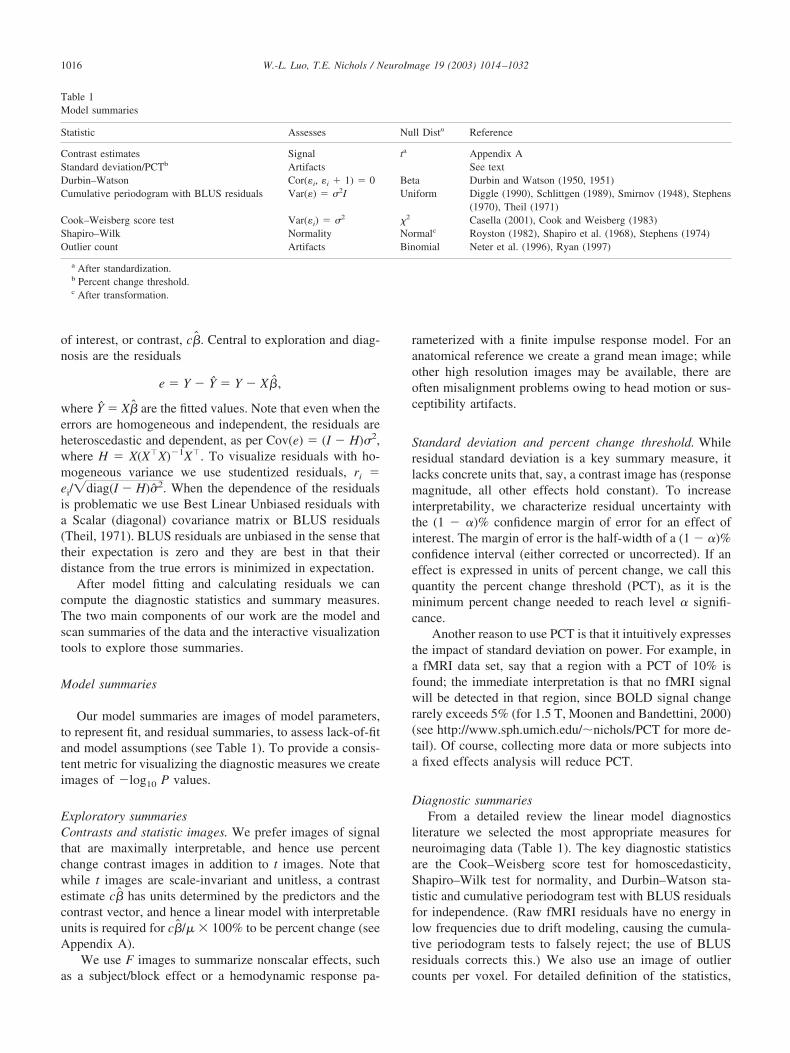
Diagnostic summariesFrom a detailed review the linear model diagnostics

literature we selected the most appropriate measures forneuroimaging data (Table 1). The key diagnostic statisticsare the Cook–Weisberg score test for homoscedasticity,Shapiro–Wilk test for normality, and Durbin–Watson sta-tistic and cumulative periodogram test with BLUS residualsfor independence. (Raw fMRI residuals have no energy inlow frequencies due to drift modeling, causing the cumula-tive periodogram tests to falsely reject; the use of BLUSresiduals corrects this.) We also use an image of outliercounts per voxel. For detailed definition of the statistics,

Table 1Model summaries

Statistic Assesses Null Distn Reference

Contrast estimates Signal ta Appendix AStandard deviation/PCTb Artifacts See textDurbin–Watson Cor(�i, �i � 1) � 0 Beta Durbin and Watson (1950, 1951)Cumulative periodogram with BLUS residuals Var(�) � �2I Uniform Diggle (1990), Schlittgen (1989), Smirnov (1948), Stephens

(1970), Theil (1971)Cook–Weisberg score test Var(�i) � �2 2 Casella (2001), Cook and Weisberg (1983)Shapiro–Wilk Normality Normalc Royston (1982), Shapiro et al. (1968), Stephens (1974)Outlier count Artifacts Binomial Neter et al. (1996), Ryan (1997)

a After standardization.b Percent change threshold.c After transformation.

1016 W.-L. Luo, T.E. Nichols / NeuroImage 19 (2003) 1014–1032

http://www.sph.umich.edu/~nichols/PCT

their distribution under a null hypothesis of model fit, andhow to assess them, please refer to Luo and Nichols (2002)and respective references.

Scan summaries

Our scan summaries are vectors where each elementassesses a single image (see Table 2). Since we do not havean explicit spatial model to evaluate, our scan summariesuse more ad hoc measures. We use the experimental pre-dictors, outlier count per scan, global signal, and someimage preprocessing parameters such as registration shiftand rotation movement parameters. These measures capturemotion, physiological, scanner artifacts or possible con-founding variables; for multisubject studies they may iden-tify anomalous subjects. While inference is not feasible onscan summaries, we do compute reference values under thenull hypothesis when possible. For example, the expectedoutlier count is easy to compute as the number of voxelstimes the Gaussian tail area of the outlier cutoffs.

Diagnosis strategies

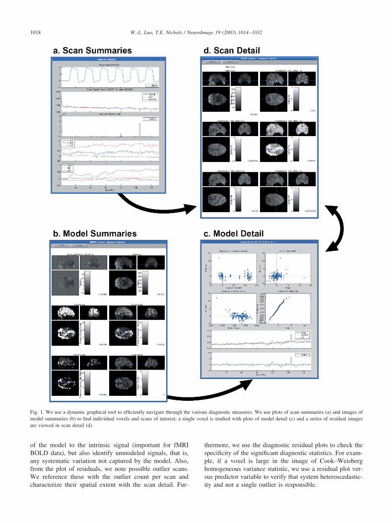
A dozen summary images and plots are an improvementover looking at every diagnostic plot and residual image, butthese summary measures are of limited use if just examinedone-by-one and not linked to the full data. Hence we use adynamic graphical tool to simultaneously view several sum-maries, linked to residual plots and images. Specifically weuse four viewers (Fig. 1) to efficiently explore the summa-ries and, as guided by the summaries, the fit and residuals.

It is not immediately clear, however, in what order thesesummaries should be examined, how the tools should beused with the summaries, and how the results of investiga-tions should be applied to the final analysis of the data. Inthis section we give an outline of strategies to simulta-neously (1) check assumptions, (2) explore expected andunexpected variability, and (3) address problems found (seeTable 3). In short, we move from summaries to detail andperform exploration and diagnosis of noise before explora-tion of signal.

Step 1: explore plots of scan summariesWe use parallel plots of scan summaries to find scans

affected by artifacts and acquisition problems (Fig. 1a). Wefirst check for systemic problems. For example, whether the

global signal is related to experimental effects or if there isexcessive movement. Second, we check for transient prob-lems, like the jumps or spikes in the global signal, theoutlier count per scan, and the motion parameters. Usually,these jumps correspond to head movements and acquisitionartifacts. Third, we check the relationships between differ-ent scan summaries, for instance, whether movement jumpsand outlier spikes coincide or if global spikes coincide withoutliers or movements. From this information, we notewhich scans are possibly corrupted or may be influential tothe data analysis. The origin of the spikes can be investi-gated in detail in Step 4.

Step 2: explore images of model summariesModel summaries are displayed next with linked orthog-

onal slice viewers (Fig. 1b) to do both diagnosis and explo-ration. In the diagnostic model summaries we pay specialattention to regions with both significant diagnostic statis-tics and anticipated experimental effects.

For exploratory purposes we search images of signaland noise, focusing on the noise first, principally with aPCT image. We window the PCT image such that themodal PCT value is half the maximal intensity (see Ap-pendix B); this gives middle gray the interpretation oftypical sensitivity and white that of less than one-halftypical sensitivity. Regions with large PCT are noted aspossible sites of Type II errors. We next check t or Fimages of nuisance effects, such as drift; with use of themodel detail, interesting features in the image of driftmagnitude can often lead to discovery of artifacts. Finallywe explore the expected signal, as measured with per-centage change, t or F images. We localize interestingactivations and note any broad patterns. In particular,extensive positive or negative regions indicate a subtlesignal (or artifact) that would not be evident in a thresh-olded statistic image. For any notable region discovered,by diagnosis or exploration, we check its model detail.

Step 3: explore model detailFor a given voxel we examine the model detail plots

(Fig. 1c), doing so interactively with images of model sum-maries to characterize the sources of the significant exper-imental or diagnostic statistics. From the plots of data withfit and residuals, we can not only assess the goodness-of-fit

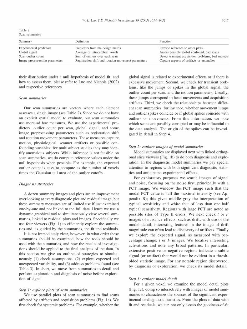
Table 2Scan summaries

Summary Definition Function

Experimental predictors Predictors from the design matrix Provide reference to other plots.Global signal Average of intracerebral voxels Assess possible global confound, bad scansScan outlier count Sum of outliers over each scan Detect transient acquisition problems, bad subjectsImage preprocessing parameters Registration shift and rotation movement parameters Capture aspects of artifacts or anomalies


of the model to the intrinsic signal (important for fMRIBOLD data), but also identify unmodeled signals, that is,any systematic variation not captured by the model. Also,from the plot of residuals, we note possible outlier scans.We reference these with the outlier count per scan andcharacterize their spatial extent with the scan detail. Fur-

thermore, we use the diagnostic residual plots to check thespecificity of the significant diagnostic statistics. For exam-ple, if a voxel is large in the image of Cook–Weisberghomogeneous variance statistic, we use a residual plot ver-sus predictor variable to verify that system heteroscedastic-ity and not a single outlier is responsible.

Fig. 1. We use a dynamic graphical tool to efficiently navigate through the various diagnostic measures. We use plots of scan summaries (a) and images ofmodel summaries (b) to find individual voxels and scans of interest; a single voxel is studied with plots of model detail (c) and a series of residual imagesare viewed in scan detail (d).


Step 4: explore scan detailAs guided by the model detail or plots of scan summa-

ries, we use a sequence of studentized residual images (Fig.1d) to spatially localize problems identified in previoussteps. Fixed and spinning maximum intensity projection(MIP) images are helpful to give an overall indication of theproblems. When examining the series of residual images,we note the spatial and temporal/interscan extent of theproblem. For example, in fMRI, an artifact confined to asingle slice in a single volume suggests shot noise, while anextended artifact may be due to physiological sources ormodel deficiencies.

Step 5: remediationSeveral approaches can be applied to address problems

identified by previous steps. For the problem scans discov-ered in Step 1, we may possibly remove them from theanalysis. We are very judicious on removing scans; we onlydiscard an observation if we are convinced that there are

deterministic measurement or execution errors (Barnett andLewis, 1994), like gross movements or spike noise. Anotherapproach to outliers is Windzorization (Wilcox, 1998), theshrinkage of outliers to the outlier threshold. In our expe-rience, outliers indicate corrupted data, and we prefer toeliminate such data rather than retaining them in modifiedform. Corresponding scans and design matrix rows must bedeleted together; the design matrix should then be checkedthat it is not exactly nor nearly rank deficient. In addition toomitting scans, we may find problem voxels in Step 2.These voxels can simply noted and ignored or explicitlymasked from the analysis.

The other approach is to modify the model. For example,if we find incorrectly modeled experimental variation fromthe model detail, we may consider adding other variables tothe model to improve the fit. In contrast, if the global signalis found to be significantly correlated with the experimentalparadigm, it may be preferable to omit this confound as acovariate entirely (Aguirre et al., 1998).

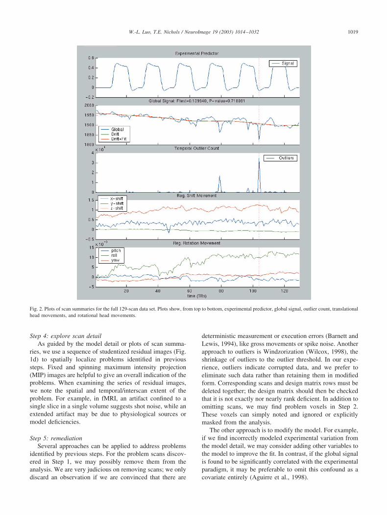
Fig. 2. Plots of scan summaries for the full 129-scan data set. Plots show, from top to bottom, experimental predictor, global signal, outlier count, translationalhead movements, and rotational head movements.


After removing possible outliers and/or modifying themodel, we refit the model and repeat the above processesagain until we are satisfied that experimental inferences arevalid and that gross artifactual variation has been omitted orat least characterized.

Step 6: resolutionAfter all the analyses and diagnoses are done, we sum-

marize the results of diagnosis and exploration. We declareeach significant region as valid, questionable or artifactual.A valid activation has assumptions clearly satisfied, while aquestionable region has some significant diagnostics butexploration of the fit and residuals has shown the activationto be believable. Artifactual activation is clearly due tooutliers or acquisition artifacts which could not be reme-died. In brain volumes with no significant activation, it isalso important to report on regions with significant diagnos-tic statistics. The source of these significant diagnostics maybe related to the unmodeled signal or artifactual variationand may be the source of new neuroscientific hypotheses, anew type of physiological signal, or simply problems forphysicists to solve.

Simulation studies

In this section we examine the performance of the modelsummary diagnostic statistics using simulated data sets. All

of our model summary statistics have been well studiedunder the null hypothesis of model fit (see respective ref-erences), so extensive simulations under the null are not inorder. Extensive evaluations under alternatives, on the otherhand, are problematic because the space of the alternativesis very large, consisting of all combinations of possibletypes model lack of fit: autocorrelation, outliers, modelmisspecification, heteroscedasticity, etc. Some evaluationsunder alternatives can be found in the references (for ex-ample, in Shapiro et al. (1968), they investigate the perfor-mance of Shapiro–Wilk under alternative distributions anddifferent sample size and show that the Shapiro–Wilk testexhibits sensitivity to nonnormality over a wide range ofalternative distributions.). Hence we only investigate thealternative of greatest concern, that of autocorrelation. Wedo this in part to demonstrate the sensitivity of our depen-dency statistics (Durbin–Watson and cumulative perio-dogram), but primarily to characterize the specificity of theother measures under the violation of their independenceassumption.

Simulation methods

Time series data were simulated from an 84-observationmodel, corresponding to a publicly available data set (http://www.fil.ion.ucl.ac.uk/spm/data), single-subject epoch audi-tory fMRI activation data; we used such a short-length timeseries to characterize the small-sample limitations of ourdiagnostic statistics. The simulated data were composed ofthe sum of two series: One was the fixed response effectincluding nine covariates corresponding to intercept, a ex-perimental condition, and seven drift terms; the other serieswas the random error, which was either white noise, afirst-order autoregressive processes with different degree ofcorrelation (0.1–0.5), or an order-12 autoregressive process.The parameters of these covariates and the 12 AR parame-ters were obtained from a real data set. A linear regressionmodel was fit to the simulated data and residuals werecreated; we computed six diagnostic statistics, Durbin–Wat-son (DW), cumulative periodogram (CP) with BLUS resid-uals (Theil, 1971), Shapiro–Wilk (SW), outliers, and twoCook–Weisberg score tests, with respect to global signal(CW-G) and predicted values (CW-P). We also calculated acumulative periodogram with ordinary residuals (CP*), in-stead of BLUS residuals.

For each type of random noise structure, we created10,000 realizations; for each realization the diagnostic sta-tistics and corresponding P values were calculated. Theperformance of the statistics were measured with two cri-teria. First, the percentages of rejection under null hypoth-esis at three rejection levels (0.05, 0.01, and 0.001) undervarious correlation conditions are computed. Second, Q–Qplots of the logarithm of the P values were created andhelpful to examine the behavior over a range of �’s.

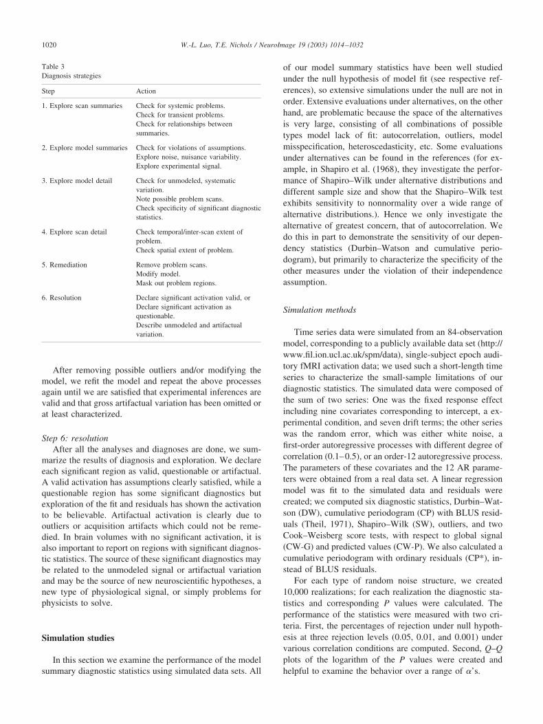
Table 3Diagnosis strategies

Step Action

1. Explore scan summaries Check for systemic problems.Check for transient problems.Check for relationships betweensummaries.

2. Explore model summaries Check for violations of assumptions.Explore noise, nuisance variability.Explore experimental signal.

3. Explore model detail Check for unmodeled, systematicvariation.Note possible problem scans.Check specificity of significant diagnosticstatistics.

4. Explore scan detail Check temporal/inter-scan extent ofproblem.Check spatial extent of problem.

5. Remediation Remove problem scans.Modify model.Mask out problem regions.

6. Resolution Declare significant activation valid, orDeclare significant activation asquestionable.Describe unmodeled and artifactualvariation.


http://www.fil.ion.ucl.ac.uk/spm/data

http://www.fil.ion.ucl.ac.uk/spm/data

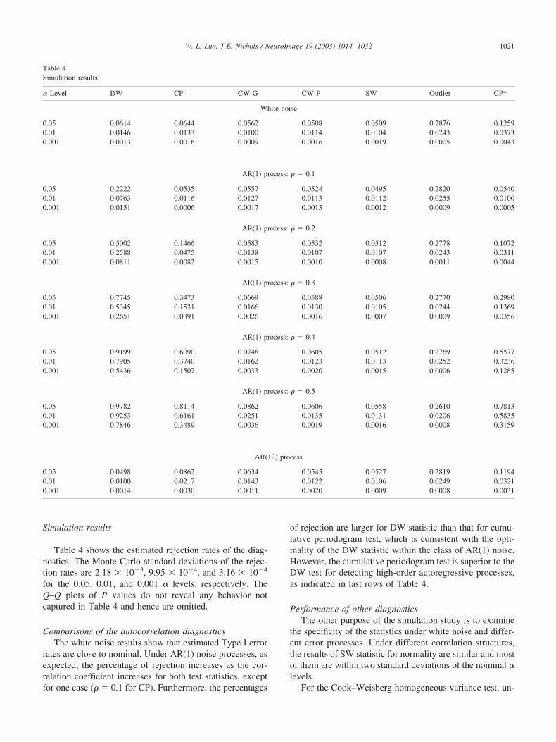
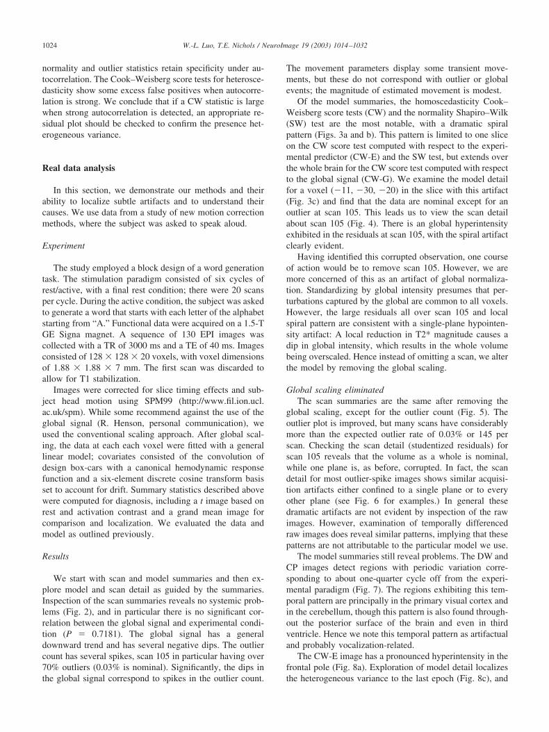
Simulation results

Table 4 shows the estimated rejection rates of the diag-nostics. The Monte Carlo standard deviations of the rejec-tion rates are 2.18 � 10�3, 9.95 � 10�4, and 3.16 � 10�4

for the 0.05, 0.01, and 0.001 � levels, respectively. TheQ–Q plots of P values do not reveal any behavior notcaptured in Table 4 and hence are omitted.

Comparisons of the autocorrelation diagnosticsThe white noise results show that estimated Type I error

rates are close to nominal. Under AR(1) noise processes, asexpected, the percentage of rejection increases as the cor-relation coefficient increases for both test statistics, exceptfor one case ( � 0.1 for CP). Furthermore, the percentages

of rejection are larger for DW statistic than that for cumu-lative periodogram test, which is consistent with the opti-mality of the DW statistic within the class of AR(1) noise.However, the cumulative periodogram test is superior to theDW test for detecting high-order autoregressive processes,as indicated in last rows of Table 4.

Performance of other diagnosticsThe other purpose of the simulation study is to examine

the specificity of the statistics under white noise and differ-ent error processes. Under different correlation structures,the results of SW statistic for normality are similar and mostof them are within two standard deviations of the nominal �levels.

For the Cook–Weisberg homogeneous variance test, un-

Table 4Simulation results

� Level DW CP CW-G CW-P SW Outlier CP*

White noise

0.05 0.0614 0.0644 0.0562 0.0508 0.0509 0.2876 0.12590.01 0.0146 0.0133 0.0100 0.0114 0.0104 0.0243 0.03730.001 0.0013 0.0016 0.0009 0.0016 0.0019 0.0005 0.0043

AR(1) process: � 0.1

0.05 0.2222 0.0535 0.0557 0.0524 0.0495 0.2820 0.05400.01 0.0763 0.0116 0.0127 0.0113 0.0112 0.0255 0.01000.001 0.0151 0.0006 0.0017 0.0013 0.0012 0.0009 0.0005


0.05 0.5002 0.1466 0.0583 0.0532 0.0512 0.2778 0.10720.01 0.2588 0.0475 0.0138 0.0107 0.0107 0.0243 0.03110.001 0.0811 0.0082 0.0015 0.0010 0.0008 0.0011 0.0044


0.05 0.7745 0.3473 0.0669 0.0588 0.0506 0.2770 0.29800.01 0.5345 0.1531 0.0166 0.0130 0.0105 0.0244 0.13690.001 0.2651 0.0391 0.0026 0.0016 0.0007 0.0009 0.0356


0.05 0.9199 0.6090 0.0748 0.0605 0.0512 0.2769 0.55770.01 0.7905 0.3740 0.0162 0.0123 0.0113 0.0252 0.32360.001 0.5436 0.1507 0.0033 0.0020 0.0015 0.0006 0.1285


0.05 0.9782 0.8114 0.0862 0.0606 0.0558 0.2610 0.78130.01 0.9253 0.6161 0.0251 0.0135 0.0131 0.0206 0.58350.001 0.7846 0.3489 0.0036 0.0019 0.0016 0.0008 0.3159

AR(12) process

0.05 0.0498 0.0862 0.0634 0.0545 0.0527 0.2819 0.11940.01 0.0100 0.0217 0.0143 0.0122 0.0106 0.0249 0.03210.001 0.0014 0.0030 0.0011 0.0020 0.0009 0.0008 0.0031


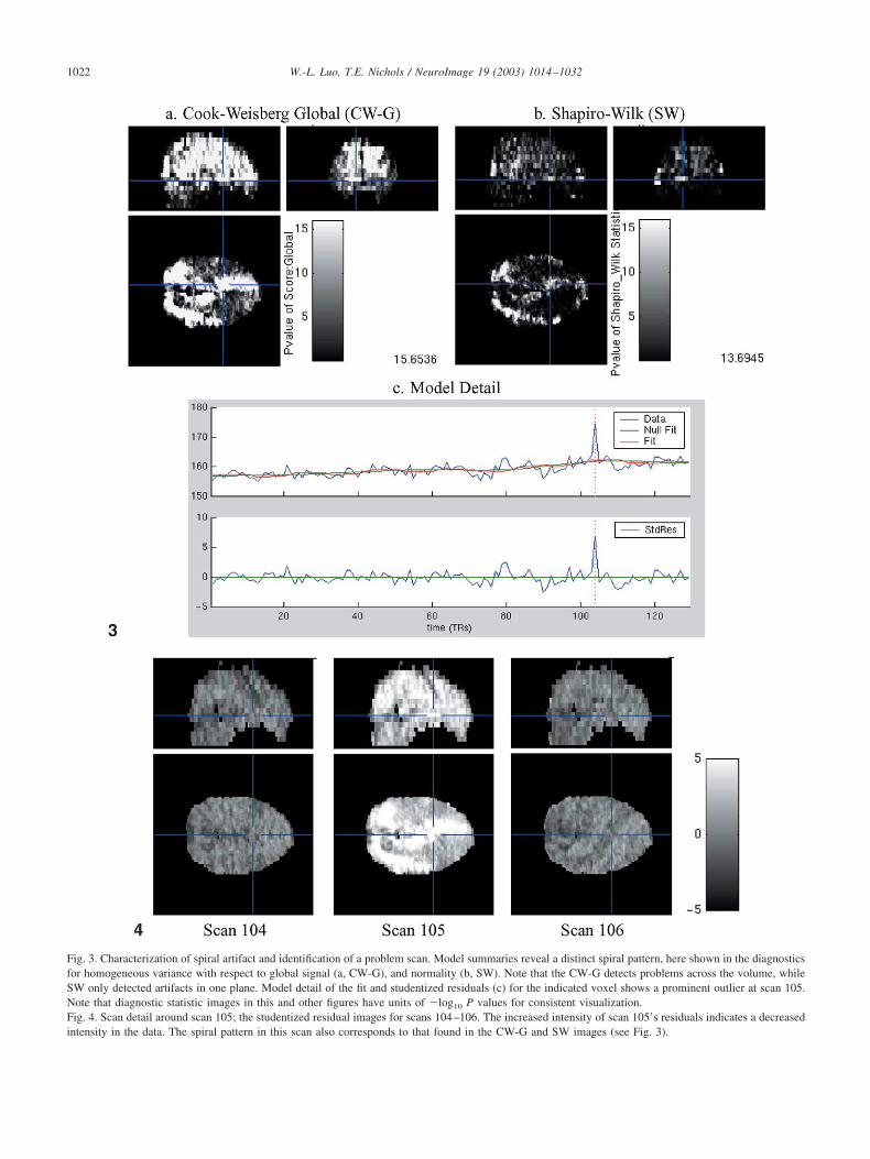
Fig. 3. Characterization of spiral artifact and identification of a problem scan. Model summaries reveal a distinct spiral pattern, here shown in the diagnosticsfor homogeneous variance with respect to global signal (a, CW-G), and normality (b, SW). Note that the CW-G detects problems across the volume, whileSW only detected artifacts in one plane. Model detail of the fit and studentized residuals (c) for the indicated voxel shows a prominent outlier at scan 105.Note that diagnostic statistic images in this and other figures have units of �log10 P values for consistent visualization.Fig. 4. Scan detail around scan 105; the studentized residual images for scans 104–106. The increased intensity of scan 105’s residuals indicates a decreasedintensity in the data. The spiral pattern in this scan also corresponds to that found in the CW-G and SW images (see Fig. 3).


der the white noise, the rejection rates are nominal for all �levels. For the AR(1) noise processes, both CW-G andCW-P tend to give estimated Type I errors that are higherthan the nominal � level. As the AR(1) process correlationincreases, the CW-G shows increasing Type I error at thethree nominal � levels, while CW-P is better, not showingappreciable anticonservativeness until � 0.3. Under theAR(12) process, the Type I errors are all slightly greaterthan the � levels.

Due to the discreteness of the outlier count, the rejectionrates are far from the nominal � � 0.05 and � � 0.01.However, comparison of the rejection rates across noiseprocesses shows that the rejection rates are quite stable,

suggesting that the outlier count is quite resilient with re-spect to autocorrelation.

The rejection rates for CP* under the white noise showsthe problem with using ordinary residuals with the cumu-lative periodogram test: For all three � levels, the CP*rejection rates are about twice the CP rates. Moreover, foralmost all dependent noise simulations, the CP rejectionrates exceeded the CP* rates. Hence these results suggestthat the cumulative periodogram test using BLUS residual isboth more specific and more sensitive than using ordinaryresiduals.

In summary, these simulation results argue that our au-tocorrelation diagnostics are specific and sensitive, that our

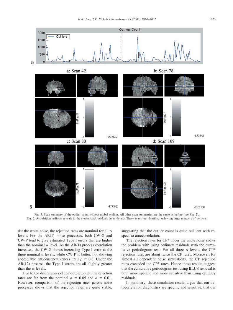
Fig. 5. Scan summary of the outlier count without global scaling. All other scan summaries are the same as before (see Fig. 2).Fig. 6. Acquisition artifacts reveals in the studentized residuals (scan detail). These scans are identified as having large numbers of outliers.


normality and outlier statistics retain specificity under au-tocorrelation. The Cook–Weisberg score tests for heterosce-dasticity show some excess false positives when autocorre-lation is strong. We conclude that if a CW statistic is largewhen strong autocorrelation is detected, an appropriate re-sidual plot should be checked to confirm the presence het-erogeneous variance.

Real data analysis

In this section, we demonstrate our methods and theirability to localize subtle artifacts and to understand theircauses. We use data from a study of new motion correctionmethods, where the subject was asked to speak aloud.

Experiment

The study employed a block design of a word generationtask. The stimulation paradigm consisted of six cycles ofrest/active, with a final rest condition; there were 20 scansper cycle. During the active condition, the subject was askedto generate a word that starts with each letter of the alphabetstarting from “A.” Functional data were acquired on a 1.5-TGE Signa magnet. A sequence of 130 EPI images wascollected with a TR of 3000 ms and a TE of 40 ms. Imagesconsisted of 128 � 128 � 20 voxels, with voxel dimensionsof 1.88 � 1.88 � 7 mm. The first scan was discarded toallow for T1 stabilization.

Images were corrected for slice timing effects and sub-ject head motion using SPM99 (http://www.fil.ion.ucl.ac.uk/spm). While some recommend against the use of theglobal signal (R. Henson, personal communication), weused the conventional scaling approach. After global scal-ing, the data at each each voxel were fitted with a generallinear model; covariates consisted of the convolution ofdesign box-cars with a canonical hemodynamic responsefunction and a six-element discrete cosine transform basisset to account for drift. Summary statistics described abovewere computed for diagnosis, including a t image based onrest and activation contrast and a grand mean image forcomparison and localization. We evaluated the data andmodel as outlined previously.

Results

We start with scan and model summaries and then ex-plore model and scan detail as guided by the summaries.Inspection of the scan summaries reveals no systemic prob-lems (Fig. 2), and in particular there is no significant cor-relation between the global signal and experimental condi-tion (P � 0.7181). The global signal has a generaldownward trend and has several negative dips. The outliercount has several spikes, scan 105 in particular having over70% outliers (0.03% is nominal). Significantly, the dips inthe global signal correspond to spikes in the outlier count.

The movement parameters display some transient move-ments, but these do not correspond with outlier or globalevents; the magnitude of estimated movement is modest.

Of the model summaries, the homoscedasticity Cook–Weisberg score tests (CW) and the normality Shapiro–Wilk(SW) test are the most notable, with a dramatic spiralpattern (Figs. 3a and b). This pattern is limited to one sliceon the CW score test computed with respect to the experi-mental predictor (CW-E) and the SW test, but extends overthe whole brain for the CW score test computed with respectto the global signal (CW-G). We examine the model detailfor a voxel (�11, �30, �20) in the slice with this artifact(Fig. 3c) and find that the data are nominal except for anoutlier at scan 105. This leads us to view the scan detailabout scan 105 (Fig. 4). There is an global hyperintensityexhibited in the residuals at scan 105, with the spiral artifactclearly evident.

Having identified this corrupted observation, one courseof action would be to remove scan 105. However, we aremore concerned of this as an artifact of global normaliza-tion. Standardizing by global intensity presumes that per-turbations captured by the global are common to all voxels.However, the large residuals all over scan 105 and localspiral pattern are consistent with a single-plane hypointen-sity artifact: A local reduction in T2* magnitude causes adip in global intensity, which results in the whole volumebeing overscaled. Hence instead of omitting a scan, we alterthe model by removing the global scaling.

Global scaling eliminatedThe scan summaries are the same after removing the

global scaling, except for the outlier count (Fig. 5). Theoutlier plot is improved, but many scans have considerablymore than the expected outlier rate of 0.03% or 145 perscan. Checking the scan detail (studentized residuals) forscan 105 reveals that the volume as a whole is nominal,while one plane is, as before, corrupted. In fact, the scandetail for most outlier-spike images shows similar acquisi-tion artifacts either confined to a single plane or to everyother plane (see Fig. 6 for examples.) In general thesedramatic artifacts are not evident by inspection of the rawimages. However, examination of temporally differencedraw images does reveal similar patterns, implying that thesepatterns are not attributable to the particular model we use.

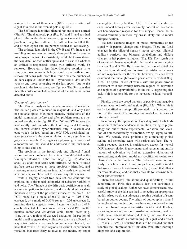
The model summaries still reveal problems. The DW andCP images detect regions with periodic variation corre-sponding to about one-quarter cycle off from the experi-mental paradigm (Fig. 7). The regions exhibiting this tem-poral pattern are principally in the primary visual cortex andin the cerebellum, though this pattern is also found through-out the posterior surface of the brain and even in thirdventricle. Hence we note this temporal pattern as artifactualand probably vocalization-related.

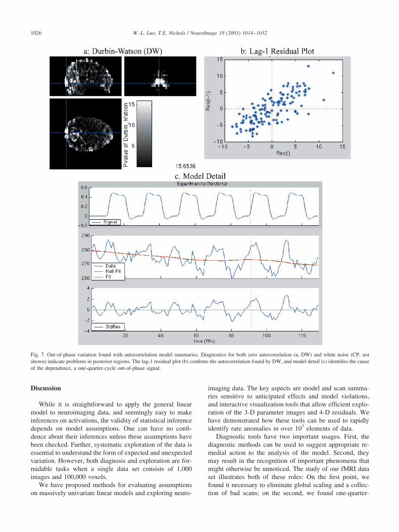
The CW-E image has a pronounced hyperintensity in thefrontal pole (Fig. 8a). Exploration of model detail localizesthe heterogeneous variance to the last epoch (Fig. 8c), and




residuals for one of these scans (109) reveals a pattern ofsignal loss also in the frontal pole (Fig. 6d).

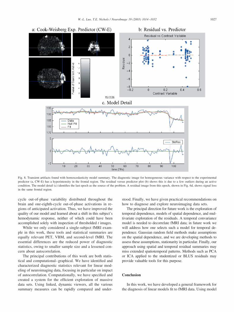
The SW image identifies bilateral regions as non-normal(Fig. 9a). The diagnostic plot (Fig. 9b) and fit and residualplots in the model detail viewer (Fig. 9c) reveal this as aproblem of negative outliers. The outliers tend to fall at theend of each epoch and are perhaps related to swallowing.

The artifacts identified in the CW-E and SW images aretroubling and we want to remedy these problems by remov-ing corrupted scans. One possibility would be to investigatethe scan detail of each outlier spike and to establish whetheran artifact is responsible; scans with artifacts would beremoved. However, a less labor-intensive solution is tosimply remove scans with large numbers of outliers. Weremove all scans with more than four times the number ofoutliers expected under the null hypothesis (1.1% or 530voxels) and those belonging to the last epoch (due to theproblem in the frontal pole, see Fig. 8c). The 34 scans thatmeet this criterion include almost all of the artifactual scansdetected above.

Corrupted scans removedThe 95-scan analysis has much improved diagnostics.

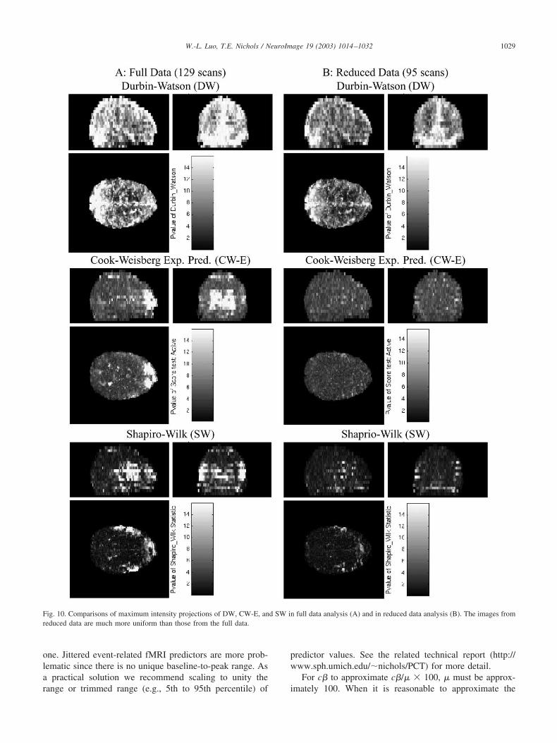
The outlier plots are reduced in magnitude and only haveone notable spike. Maximum intensity projections of themodel summaries before and after problem scans are re-moved are shown in Fig. 10. The CW and SW images arenow mostly uniform, while the DW image and CP image(not shown) exhibit hyperintensities only in vascular andedge voxels. In fact, based on a 0.05-FDR-thresholded im-ages (not shown), the autocorrelation is only significant ingray matter voxels. This suggests a physiological source ofautocorrelation that should be addressed in the final mod-eling of this data set.

The problems in the frontal pole and bilateral frontalregions are much reduced. Inspection of model detail at thefew hyperintensities in the SW image (Fig. 9b) identifiesabout six additional scans with artifacts. As none of theseartifacts are as severe as those previously identified, andsince any removal of outliers invariably leads to creation ofnew outliers, we chose not to remove any other scans.

With a largely artifact-free data set, we continue ourexploration of the model summaries of nuisance variabilityand noise. The F image of the drift basis coefficients revealsno unusual patterns (not shown) and mainly identifies slowmonotonic drifts at the posterior surface of the brain. ThePCT image has a mode of 0.47% (for � � 0.05 FDR-corrected, or a mode of 0.30% for � � 0.05 uncorrected),meaning that in a typical voxel changes as small as 0.47%can be detected. Of concern is the increased PCT in thebilateral motor and left dorsal lateral frontal areas (Fig.11a), the very regions of expected activation. Inspection ofmodel detail suggests that, while a few scans are affected byacquisition artifacts, no problems are severe. Instead, wenote that voxels in these regions all exhibit experimentalvariation that rises early relative to the model, by about

one-eighth of a cycle (Fig. 11c). This could be due toexperimental timing errors or simply poor fit of the canon-ical hemodynamic response for this subject. Hence the in-creased variability in these regions is likely due to modelmisspecification.

We next examine images of model summaries of thesignal with percent change and t images. There are focalchanges in the bilateral sensory–motor cortices, bilateralauditory cortices, and bilateral cerebellum and diffusechanges in left prefrontal regions (Fig. 12). The signals areof expected change magnitude, the local maxima rangingbetween 3 and 5.5%. By examining the model detail foreach foci (not shown), we confirm that artifactual sourcesare not responsible for the effects; however, for each voxelexamined the one-eighth-cycle phase error is evident (Fig.11c). The spatial extent of voxels with this phase error isconsistent with the overlap between regions of activationand regions of hypervariability in the PCT, suggesting thatlack of fit is responsible for the increased residual variabil-ity.

Finally, there are broad patterns of positive and negativechanges about orbitofrontal regions (Fig. 12a). While this iseasily identified as susceptibility-related, it is a demonstra-tion of the merit of examining unthresholded images ofestimated signal.

In summary, the application of our diagnostic tools findsviolation of the independence assumption, owing to physi-ology and out-of-phase experimental variation, and viola-tion of homoscedasticity assumption, owing largely to arti-facts. We remedy these problems by eliminating globalscaling and removing scans with serious artifacts. The re-sulting reduced data set is satisfactory, except for typicalfMRI autocorrelation in gray matter and vascular regions. Inregions of activation we find no extensive violations ofassumptions, aside from model misspecification owing to aphase error in the predictor. The reduced dataset is nowready for a final model fitting, in particular, with a modelthat uses a shorter hemodynamic delay (or one that allowsfor variable delay) and one that accounts for intrinsic tem-poral autocorrelation.

There are several limitations and qualifications to thisdemonstration. First, this analysis does not constitute astudy of global scaling. Rather we have demonstrated howcareful study of the data can lead to selecting an appropriatemodel. Also, we do not advocate a routine deletion of scansbased on outlier counts. The origin of outlier spikes shouldbe explored and understood; we have only removed scanswhen an obvious acquisition artifact is identified. Further,removing scans is just one possible remediation, and wecould have instead Windzorized. Finally, we note that vo-calization can create a confounding of signal and artifact(Birn et al., 1998), a situation that is to be avoided and thattroubles the interpretation of this data even after thoroughdiagnosis and exploration.


Discussion

While it is straightforward to apply the general linearmodel to neuroimaging data, and seemingly easy to makeinferences on activations, the validity of statistical inferencedepends on model assumptions. One can have no confi-dence about their inferences unless these assumptions havebeen checked. Further, systematic exploration of the data isessential to understand the form of expected and unexpectedvariation. However, both diagnosis and exploration are for-midable tasks when a single data set consists of 1,000images and 100,000 voxels.

We have proposed methods for evaluating assumptionson massively univariate linear models and exploring neuro-

imaging data. The key aspects are model and scan summa-ries sensitive to anticipated effects and model violations,and interactive visualization tools that allow efficient explo-ration of the 3-D parameter images and 4-D residuals. Wehave demonstrated how these tools can be used to rapidlyidentify rare anomalies in over 107 elements of data.

Diagnostic tools have two important usages. First, thediagnostic methods can be used to suggest appropriate re-medial action to the analysis of the model. Second, theymay result in the recognition of important phenomena thatmight otherwise be unnoticed. The study of our fMRI dataset illustrates both of these roles: On the first point, wefound it necessary to eliminate global scaling and a collec-tion of bad scans; on the second, we found one-quarter-

Fig. 7. Out-of-phase variation found with autocorrelation model summaries. Diagnostics for both zero autocorrelation (a, DW) and white noise (CP, notshown) indicate problems in posterior regions. The lag-1 residual plot (b) confirms the autocorrelation found by DW, and model detail (c) identifies the causeof the dependence, a one-quarter-cycle out-of-phase signal.


cycle out-of-phase variability distributed throughout thebrain and one-eighth-cycle out-of-phase activations in re-gions of anticipated activation. Thus, we have improved thequality of our model and learned about a shift in this subject’shemodynamic response, neither of which could have beenaccomplished solely with inspection of thresholded t images.

While we only considered a single-subject fMRI exam-ple in this work, these tools and statistical summaries areequally relevant PET, VBM, and second-level fMRI. Theessential differences are the reduced power of diagnosticstatistics, owing to smaller sample size and a lessened con-cern about autocorrelation.

The principal contributions of this work are both statis-tical and computational–graphical. We have identified andcharacterized diagnostic statistics relevant for linear mod-eling of neuroimaging data, focusing in particular on impactof autocorrelation. Computationally, we have specified andcreated a system for the efficient exploration of massivedata sets. Using linked, dynamic viewers, all the varioussummary measures can be rapidly compared and under-

stood. Finally, we have given practical recommendations onhow to diagnose and explore neuroimaging data sets.

The principal direction for future work is the exploration oftemporal dependence, models of spatial dependence, and mul-tivariate exploration of the residuals. A temporal convariancemodel is needed to decorrelate fMRI data; in future work wewill address how one selects such a model for temporal de-pendence. Gaussian random field methods make assumptionson the spatial dependence, and we are developing methods toassess these assumptions, stationarity in particular. Finally, ourapproach using spatial and temporal residual summaries maymiss extended spatiotemporal patterns. Methods such as PCAor ICA applied to the studentized or BLUS residuals mayprovide valuable tools for this purpose.

Conclusion

In this work, we have developed a general framework forthe diagnosis of linear models fit to fMRI data. Using model

Fig. 8. Transient artifacts found with homoscedasticity model summary. The diagnostic image for homogeneous variance with respect to the experimentalpredictor (a, CW-E) has a hyperintensity in the frontal region. The residual versus predictor plot (b) shows this is due to a few outliers during an activecondition. The model detail (c) identifies the last epoch as the source of the problem. A residual image from this epoch, shown in Fig. 6d, shows signal lossin the same frontal region.


and scan summaries and dynamic linked viewers, we haveshown how to swiftly localize rare anomalies and artifactsin large 4-D data sets.

Acknowledgments

The authors thank Brian Ripley and Philip Howrey forvaluable conversations about this work. We also thank BoklyeKim for using the example data and John Ashburner for cre-ating the orthogonal viewer tool used extensively in our software.

Appendix A

Percent change and interpretable linear models

This appendix shows how to create interpretable linearmodels, from which it is easy to create percent changecontrast images. Neuroimaging linear models are tradition-

ally not constructed to yield maximally interpretable param-eters. For example, the standard two-sample t test, imple-mented with a zero–one design matrix and c � [�1 1],yields a c� with half-magnitude units. Here we show how toscale X and c such that c� has the same units as the data andthat c�/� � 100 has percent change units; if the data areintensity normalized, c� can approximate percent change.

The two key requirements are that (1) each column, Xj

corresponding to an experimental effect represent a unitchange in the data and (2) contrasts have absolute sum of unity.Condition 1 ensures that a unit change in �j corresponds to aunit change in Y, and condition 2 ensures that these units arepreserved. While condition 2 is easy to enforce in software,condition 1 requires care while constructing predictors.

Categorical predictors will satisfy condition 1 when the“off” to “on” difference is unity, such as coding dummyvariables with 0 and 1 (but not -1 and 1). In block-designfMRI, this requires the that baseline-to-activation be scaledto unity, and in event-related fMRI with isolated or equallyspaced events, the baseline to peak height can be scaled to

Fig. 9. Periodic artifacts found with the normality model summary. The normality diagnostic (a, SW) is mostly nominal, except in in bilateral frontal regions.The Q–Q plot of one of these nonnormal voxels (b) shows that many negative outliers are responsible, and the model detail (c) shows these outliers areregularly spaced with roughly the experimental periodicity.


one. Jittered event-related fMRI predictors are more prob-lematic since there is no unique baseline-to-peak range. Asa practical solution we recommend scaling to unity therange or trimmed range (e.g., 5th to 95th percentile) of

predictor values. See the related technical report (http://www.sph.umich.edu/�nichols/PCT) for more detail.

For c� to approximate c�/� � 100, � must be approx-imately 100. When it is reasonable to approximate the

Fig. 10. Comparisons of maximum intensity projections of DW, CW-E, and SW in full data analysis (A) and in reduced data analysis (B). The images fromreduced data are much more uniform than those from the full data.




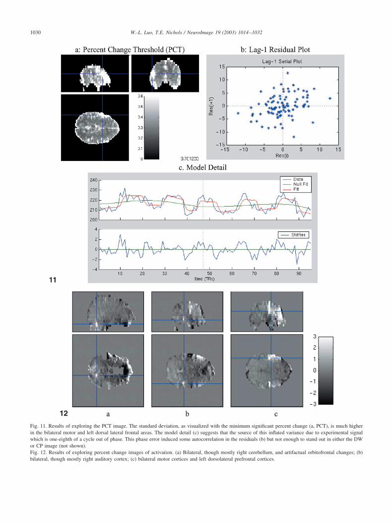
Fig. 11. Results of exploring the PCT image. The standard deviation, as visualized with the minimum significant percent change (a, PCT), is much higherin the bilateral motor and left dorsal lateral frontal areas. The model detail (c) suggests that the source of this inflated variance due to experimental signalwhich is one-eighth of a cycle out of phase. This phase error induced some autocorrelation in the residuals (b) but not enough to stand out in either the DWor CP image (not shown).Fig. 12. Results of exploring percent change images of activation. (a) Bilateral, though mostly right cerebellum, and artifactual orbitofrontal changes; (b)bilateral, though mostly right auditory cortex; (c) bilateral motor cortices and left dorsolateral prefrontal cortices.


baseline (grand mean) image with a constant (e.g., in fMRI),all data are scaled such that the baseline images’ “global”intensity is 100. But we find that the usual global estimate,the arithmetic mean of all intracerebral voxels, is unsatis-factory. The mean is sensitive to hyperintensity outliers andthe segmentation of brain from nonbrain. If a simple inten-sity threshold is used to segment brain and the threshold isset too low, the global average can be far below typicalbrain intensities. We propose that the mode is a more ac-curate global measure than the mean, as the mode is veryrobust with respect to brain threshold. In Appendix B wegive a method to estimate the intracerebral mode.

To summarize, we assert that models should be con-structed to be as interpretable as possible. The rewards ofthis endeavor are that, if the voxel grand means are around100, the predictors have unit scaling, and the contrast vectorhas an absolute sum of unity, then the contrast image willhave approximate interpretation of percent change. Ratioingsuch a contrast image with a grand mean image will producepercent change exactly.

Appendix B

Estimation of the intracerebral modal intensity

This appendix describes the estimation of the mode ofintracerebral voxel intensities. This method consists of es-timating a brain–nonbrain threshold and then estimating themode of the distribution of brain voxel intensities. Whilethere is an extensive literature on mode estimation usingkernel density estimation (see, e.g., Scott, 1992), we simplyuse a histogram estimate with appropriate bin widths for aconsistent estimator1 of the mode. Our approach uses notopological operations on the image data and is easily codedand quickly computed.

Estimating brain–nonbrain threshold with the antimodeWe estimate a brain–nonbrain threshold using the distri-

bution of all voxel intensities. Our threshold is the locationof minimum density between the background and gray mat-ter modes; call this the antimode. Let f(x) be the distributionof intensities in the brain image. Hartigan (1977) shows thata consistent estimator of the antimode is the location of themaximally separated order statistic between modes. Sincewe do not know the location of modes, we instead justsearch over the whole density excluding the tails; the tailsmust be excluded as the global minimum of f(x) will befound there. A crude overestimate of the tails is sufficient,since the antimode estimate will only be perturbed if weinclude tails with less density than the antimode or excludethe actual location of the antimode. We have found the 10th

and 90th percentiles to work on all images we have consid-ered. Our threshold estimate is thus

T � �1

2� x�k�1� � x�k�� : k � argmax

0.1ni0.9n

� x�i�1� � x�i�� ,

(1)

where n is the number of voxels in the image and x(k) is thek-th order statistic. If k is not unique, we take an average ofthe locations.

While this works well on continuous-valued image (e.g.,a floating point mean image), it does not work with adiscrete-valued image (e.g., an integer T2* image). Theproblem is that the distance between order statistics will be0 or 1 except at the very extreme tails. Hence if the imageis discrete we then revert to a simpler histogram method.We construct a histogram based on all nontail data (10th to90th percentile) and use the location of the minimum bin asthe antimode estimate. To construct the histogram we usethe bin width rule for the mode (described below). We havefound that this serves as a robust estimate of a brain–nonbrain threshold.

Whether through the inter-order-statistic distance or the

1 With more and more data, a consistent estimator converges to the truevalue in probability.

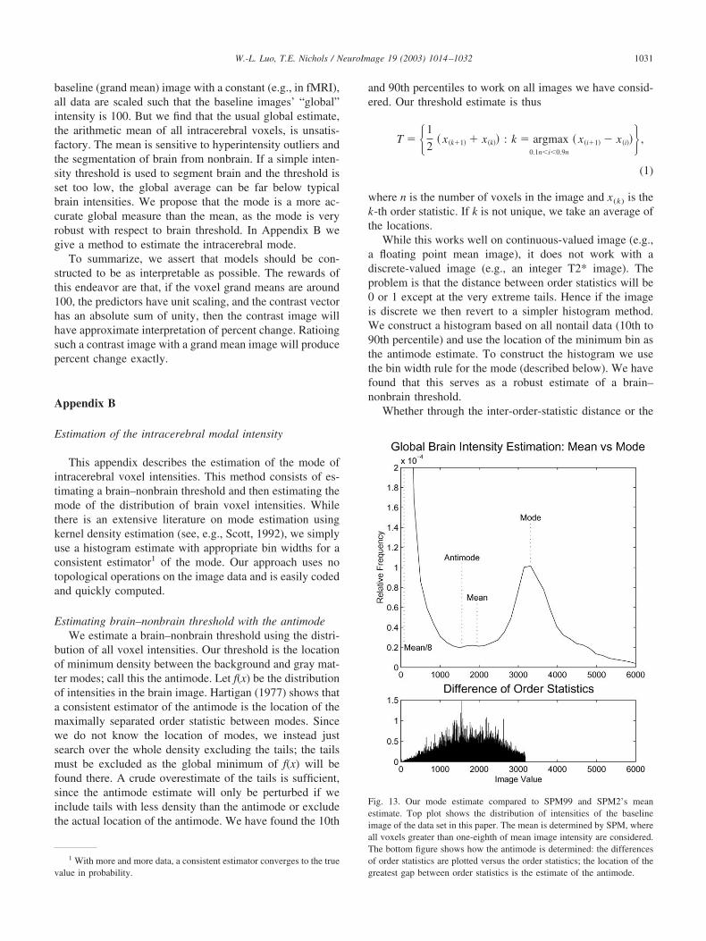
Fig. 13. Our mode estimate compared to SPM99 and SPM2’s meanestimate. Top plot shows the distribution of intensities of the baselineimage of the data set in this paper. The mean is determined by SPM, whereall voxels greater than one-eighth of mean image intensity are considered.The bottom figure shows how the antimode is determined: the differencesof order statistics are plotted versus the order statistics; the location of thegreatest gap between order statistics is the estimate of the antimode.


histogram approach, this antimode estimate is only used toeliminate the lower mode of background voxels and hencedoes not need to be highly accurate.

Estimating global brain intensity with the modeWe estimate the mode of the brain voxel intensities using

a type of histogram estimate for simplicity and computa-tional efficiency. The optimal (and consistent) histogrambin width for estimating the mode is order n1/5; we use binwidths equal to 1.595 � IQRn�1/5 (Scott, 1992, p100),where IQR is the interquartile range of the brain voxels.While this rule is based on independent normal data, it hasperformed quite well on many PET and fMRI data sets. Themode estimate is the location of the maximal histogram bin.

While we do not argue that this mode estimate is optimal inthe sense of mean squared error, we have found it to be robustand sufficiently accurate for the purposes of this work. Inparticular, we have found it more accurate than the simple esti-mator used in SPM (see Fig. 13). Matlab code for this method isavailable at http://www.sph.umich.edu/�nichols/PCT.

References

Aguirre, G.K., Zarahn, E., D’Esposito, M., 1998. The inferential impact ofglobal signal covariates in functional neuroimaging analyses. Neuro-Image 8, 302–306.

Ashburner, J., Friston, K.J., 2000. Voxel-based morphometry—the meth-ods. NeuroImage 11, 805–821.

Barnett, V., Lewis, T., 1994. Outliers in Statistical Data, third ed. Wiley,New York.

Birn, R.M., Bandettini, P.A., Cox, R.W., Jesmanowicz, A., Shaker, R.,1998. Magnetic field changes in the human brain due to swallowing orspeaking. Magn. Reson. Med. 40, 55–60.

Burock, M.A., Dale, A.M., 2000. Estimation and detection of event-relatedfMRI signals with temporally correlated noise: a statistically efficientand unbiased approach. Hum. Brain Map. 11, 249–260.

Casella, G., 2001. Statistical Inference, second ed. Wadsworth, Belmont, CA.Cook, R.D., Weisberg, S., 1983. Diagnostics for heteroscedasticity in

regression. Biometrika 70, 1–10.Diggle, P.J., 1990. Time Series: A Biostatistical Introduction. Oxford

University Press, Oxford.Draper, N.R., Smith, H., 1998. Applied Regression Analysis, third ed.

Wiley, New York.Friston, K.J., Holmes, A.P., Worsley, K.J., Poline, J.-B., Frackowiak,

R.S.J., 1995. Statistical parametric maps in functional imaging: a gen-eral linear approach. Hum. Brain Map. 2, 189–210.

Goutte, C., Toft, P., Rostrup, E., Nielsen, F.A., Hansen, L.K., 1999. Onclustering fMRI time series. NeuroImage 9, 298–310.

Hartigan, J.A. 1977. Distribution problems in clustering, in: Classificationand Clustering, Academic Press, New York/London, pp. 45–72.

Hoaglin, D.C., Mosteller, F., Tukey, J.W. (Eds.), 1983. UnderstandingRobust and Exploratory Data Analysis, Wiley, New York.

Holmes, A.P. 1994. Statistical Issues in Functional Brain Mapping, Ph.D.thesis. University of Glasgow. Available from: http://www.fil.ion.ucl.ac.uk/spm/papers/APH_thesis.

Holmes, A.P., Friston, K.J., 1999. Generalisability, random effects andpopulation inference. NeuroImage 7 (4 (2/3)), S754.

Kherif, F., Poline, J.-B., Flandin, G., Benali, H., Simon, O., Dehaene, S.,Worsley, K.J., 2002. Multivariate model specification for fMRI data.NeuroImage 16 (4), 1068–1083.

Luo, W.-L., Nichols, T.E. 2002. Diagnosis and Exploration of MassivelyUnivariate fMRI Models, technical report. Department of Biostatistics,University of Michigan.

McKeown, M.J., Makeig, S., Brown, G.G., Jung, T-P., Kindermann, S.S.,Bell, A.J., Sejnowski, T.J., 1998. Analysis of fMRI data by blind separa-tion into independent spatial components. Hum. Brain Map. 6, 160–188.

Moonen, C.T.W., Bandettini, P.A. (eds.), 2000. Functional MRI. SpringerVerlag, New York.

Moser, E., Baumgartner, R., Barth, M., Windischberger, C., 1999. Explor-ative signal processing in functional MR imaging. Int. J. Imag. Syst.Technol. 10, 166–176.

Neter, J., Kutner, M.H., Nachtsheim, C.J., Wasserman, W., 1996. AppliedLinear Statistical Models, fourth ed. Irwin, Chicago, IL.

Nichols, T.E., Luo, W.L., 2001. Data exploration through model diagnosis.NeuroImage 13 (6(2/2)), S208.

Petersson, K.M., Nichols, T.E., Poline, J.-B., Holmes, A.P., 1999. Statis-tical limitations in functional neuroimaging. II. Signal detection andstatistical inference. Phil. Trans. R. Soc. Lond. B 354, 1261–1281.

Razavi, M., Grabowski, T.J., Mehta, S., Bolinger, L., 2001. The source ofresidual temporal autocorrelation in fMRI time series. NeuroImage 13(6(2/2)), S228.

Royston, J.P., 1982. An extension of Shapiro and Wilk’s W test fornormality to large samples. Appl. Stat. 31, 115–124.

Ryan, T.P., 1997. Modern Regression Methods. Wiley-Interscience, NewYork.

Schlittgen, R., 1989. Tests for white noise in the frequency domain.Comput. Stat. 4, 281–288.

Scott, D.W., 1992. Multivariate Density Estimation: Theory, Practice, andVisualization. Wiley, New York.

Shapiro, S.S., Wilk, M.B., Chen, H.J., 1968. A comparative study ofvarious tests for normality. J. Am. Stat. Assoc. 63, 1343–1372.

Smirnov, N., 1948. Table for estimating the goodness of fit of empiricaldistributions. Ann. Math. Stat. 19 (2), 279–281.

Stephens, M.A., 1970. Use of the Kolmogorov-Smirnov, Cramer-vonMises and related statistics without extensive tables. J. R. Stat. Soc.Ser. B Methodol. 32, 115–122.

Stephens, M.A., 1974. EDF statistics for goodness of fit and some com-parisons. J. Am. Stat. Assoc. 69, 730–737.

Theil, H., 1971. Principles of Econometrics. J Wiley, New York.Tukey, J.W., 1977. Exploratory Data Analysis. Addison-Wesley, Reading, MA.Wilcox, R. 1998. in: Trimming and winsorization, Encyclopedia of Bio-

statistics, Vol. 6. Wiley, New York, pp. 4588–4590.Woolrich, M.W., Ripley, B.D., Brady, M., Smith, S., 2001. Temporal

autocorrelation in univariate linear modeling of fMRI data. NeuroIm-age 14, 1370–1386.



http://www.fil.ion.ucl.ac.uk/spm/papers/APH_thesis

http://www.fil.ion.ucl.ac.uk/spm/papers/APH_thesis

Diagnosis and exploration of massively univariate ... - CiteSeerX

Documents