DETERMINANTS OF THE FUNDING VOLATILITY OF INDONESIAN BANKS: A DYNAMIC MODEL

DETERMINANTS OF THE FUNDING VOLATILITY OF INDONESIAN BANKS: A DYNAMIC MODEL

James Obben and Agus Eko Nugroho

Discussion Paper No. 03.07 – 2003

Massey University DEPARTMENT OF APPLIED AND INTERNATIONAL ECONOMICS

DETERMINANTS OF THE FUNDING VOLATILITY OF

INDONESIAN BANKS: A DYNAMIC MODEL

James Obben*1 and Agus Eko Nugroho**

*Department of Applied and International Economics Massey University Private Bag 11-222 Palmerston North

New Zealand E-mail: [email protected]

and

**The Indonesian Institute of Sciences

Jakarta Indonesia

ABSTRACT Illiquidity is at the core of the various currency and banking/financial crises of the 1990s. In the wake of the Asian crisis of 1997/98 the term “systemic liquidity” has been coined to refer to adequate arrangements and practices which permit efficient liquidity management and which provide a buffer during financial distress. A constructed balance-sheet-based variable that captures the essence of the risk from systemic liquidity is funding volatility ratio, FVR. Using data covering January 1990 to July 2003 and employing cointegration techniques, this study attempts to quantify the purported link between FVR and the measurable determinants of a balanced liquidity infrastructure for Indonesia, the country that suffered the most from the Asian crisis. A good fit is obtained for the dynamic regression model and estimates of short-run and long-run impacts and elasticities are computed. FVR is shown to be increasing in the rupiah-US dollar exchange rate, the Jakarta stock market index, interest rate and the number of banks, and decreasing in capital:asset ratio and foreign liabilities: total asset ratio. The best option for lowering the FVR in the short run is increasing bank capital; over the long term enduring increases in foreign-currency accounts and reduction in the number of banks seem to hold the best prospect for lowering the FVR.

Keywords: autoregressive distributed lag model; cointegration; funding volatility ratio; systemic liquidity.

JEL classification: C22; G21; N25.

1 Corresponding author. The modelling approach benefited from discussions with Jen-Je Su and Rukmani Gounder. The usual caveat applies.

1. INTRODUCTION The theory of banking is well established and widely known. Banks exist to intermediate between cash-surplus economic agents and cash-deficit agents with profitable investment opportunities. To achieve the multi-faceted objective of optimizing profitability, liquidity and solvency, banks manage their assets, liabilities, liquidity and capital adequacy by minimising the risk they face from loan default (credit risk), deposit withdrawals (liquidity risk) and interest rate movements that can reduce their earnings and returns (interest-rate risk). Where foreign-currency transactions are significant there might be the additional risk from adverse exchange rate movements to contend with. Excessive risk taking or ineffectual risk management by banks, ineffective supervision by regulatory agencies and matters that undermine depositors’ and creditors’ confidence are at the core of all bank failures. Because of the special importance of well-functioning banks and bank credit to economic activity, banks are heavily regulated. For further details the reader is referred to Mishkin (1998). In the wake of the Asian crisis2 of 1997/98, considered to be the most significant among the currency and banking/financial crises of the 1990s, and given the pernicious illiquidity attendant to those episodes, there has been renewed interest in the importance of banks’ access to liquid funding markets and sound bank liquidity management for the resilience of national financial systems and for the international financial system as well (Enoch et al., 2002; Keller et al., 2002; and World Bank Policy Report, 2001).3 For instance, the working group of finance ministers and central bank governors from 22 systemically at-risk countries deliberating ways for strengthening national financial systems emphasized the modalities for liquidity and coined the term “systemic liquidity” to refer to adequate arrangements and practices which permit efficient liquidity management and which provide a buffer during financial distress (Group of 22, 1998). In further elucidation of the term, Dziobek, Hobbs and Marston (2000, 2002), hereafter DHM, proffer that systemic liquidity can be viewed as the combination of bank liquidity management practices and the supporting liquidity infrastructure. Bank liquidity management practices are those confidence-enhancing practices aimed at providing the bank and its customers with the assurance that the bank’s liability obligations can be met as they become due without necessarily having to roll over these or postpone access to credit. In the event, the threat to the bank’s viability from loss of 2 Accounts of the causes of the Asian crisis may be gleaned from papers such as Berg and Patillo (1999), Corsetti et al. (1998a,b,c), Furman and Stiglitz (1998), Kaminsky and Reinhart (1999), Montes (1998), and Radelet and Sachs (1998). Those dealing more specifically with Indonesia are Cole and Slade (1998), Djiwandono (2001) and Nasution (1999). 3 The currency and banking/financial crises of the 1990s undoubtedly spawned a lot of theoretical and empirical literature on financial systems. The subset of the literature dealing with tools to recognize symptoms of financial crises may be divided into two: early warning systems (EWS) and balance sheet approaches. The EWS studies seek to outline the linkages between currency and banking/financial crises and identify and characterise the behaviour of likely leading indicators of currency crises for groups of nations and generalize from that (e.g., Eichengreen et al. 1995; Sachs et al. 1996; Frankel and Rose 1996; Kaminsky, Lizondo and Reinhart 1998; and Kaminsky and Reinhart 1998, 1999). Countries are lumped together thus masking the unique characteristics of each country’s experience. The balance-sheet-based studies investigate the liquidity risk and imbalances pertaining to asset-liability maturity and currency mismatches and capital structure distortions in the banking and corporate sectors as well as the government’s budget (e.g., Keller et al. 2002). Since the subjects in these latter studies are individual countries the policy recommendations may be better attuned to the countries’ unique characteristics. It is obvious that this study belongs to the balance-sheet genre.

1

liquidity or confidence becomes a function of the volatility of funding relative to the liquidity of bank assets. Funding volatility refers to the likelihood that bank depositors or creditors will, in a short period of time, withdraw their funds or fail to roll them over at maturity in response to a perceived weakness in an individual bank or banking system. The term liquidity infrastructure is used to summarise (i) the design and adequacy of prudential rules and monetary instruments, (ii) the existence of legal contract rights and the efficiency of the court system, (iii) foreign exchange regulations, (iv) variability of interest rates, (v) exchange rates and (vi) safety-net provisions. DHM expound on these cogently. A balance-sheet-based indicator of funding volatility for the entire banking system advocated by DHM is funding volatility ratio (FVR) defined as the ratio of the difference between banks’ volatile liabilities and liquid assets to the banks’ illiquid assets. FVR reflects banks’ dependence on confidence-sensitive funds and is ostensibly closely linked to the six above-mentioned factors that affect a balanced liquidity infrastructure. DHM stress that estimated FVRs should be interpreted in the context of the infrastructure for liquidity management and hence in their analysis of the FVRs of the banking systems of 14 countries covering the 1992-98 period they underscore the link by reporting for each country the average FVR for the study period and map out the infrastructure at end-1997. Difficulties with data issues are noted. Additionally, they outline the rudiments of a four-quadrant classification scheme that can be used to categorise countries according to their scores on FVR (on the vertical axis) and some yet-to-be defined composite index of balanced infrastructure (on the horizontal axis). There is no explicit quantification of the link between FVR and the factors that affect a balanced liquidity infrastructure. Rather than interpreting the estimated FVR against the backdrop of the prevailing liquidity infrastructure, we are interested in the extent to which the FVR depends on the factors driving the liquidity infrastructure. Such an analytical endeavour can help delineate the relative importance of the various factors by way of the elasticity measures that can be calculated therefrom. In this study we seek to quantify that link for Indonesia, the country that suffered the most from the Asian crisis and is also one of the 14 countries investigated by DHM. We use monthly data covering 1990:01 to 2003:07 and employ cointegration techniques. To our knowledge no such study has been undertaken that can bring its unique insights to bear on the systemic liquidity policy in a country still having significant bank restructuring problems.4 The study borrows heavily from DHM to construct the required variables but draws inspiration from Coe and Helpman (1995) who quantified the purported link between total factor productivity (TFP) and research and development (R&D) capital stocks for 21 OECD countries plus Israel during the period 1971-90. In the rest of the paper, we discuss the construction and theoretical relationships among the variables and outline the main features of the chosen autoregressive distributed lag (ARDL) model in Section 2. A description of the data and the estimation procedures we took are recounted in Section 3. Section 4 presents and discusses the empirical results and Section 5 contains the summary and conclusions.

4 See Pangestu and Habir (2002a,b) for a comprehensive up-to-date review of the performance, regulation and prospects of Indonesian banks.

2

2. VARIABLE CONSTRUCTION AND MODEL SPECIFICATION The Funding Volatility Ratio DHM define funding volatility ratio as:

FVR = (VL – LA) / (TA – LA) where VL is volatile liabilities; LA is liquid assets; and TA is total assets. With the caveat that the liquidity properties of assets and liabilities depend on the institutional setting DHM reported the following compositions of their variables: LA = cash + trading, short-term marketable and government securities + claims due from banks; VL = total borrowed funds; and TA = reported assets + off-balance sheet items + consumer liabilities on acceptance and bills rediscounted. Given the available Indonesian data and institutional setting we constructed the constituent variables in the FVR formula in the following way: LA = cash + reserves + capital; VL = saving and demand deposits + foreign liabilities + import guarantees; and TA = total assets. The implications of the values that FVR can take are: FVR = 0 implies volatile liabilities are fully covered by liquid assets; FVR < 0 implies volatile liabilities are more than fully covered by liquid assets; and FVR > 0 implies volatile liabilities are not fully covered by liquid assets. Hence, positive, zero and negative values for FVR indicate, respectively, high, intermediate and low systemic liquidity risk. With respect to the dynamic behaviour of FVR we can note that since at period t, FVRt = (VLt – LAt) / (TAt – LAt) then the value of FVR at some later time t + ∆t is given by:

tt

tt

tt

tttt LATA

LALAVLVLLALALATALALAVLVL

FVR−

∆+−∆+=

∆+−∆+∆+−∆+

=∆+

)()()()()()(

where the difference operator ∆ is used to denote discrete change in a variable. FVR decreases when the numerator gets smaller relative to the denominator, which can come about when either (i) LA increases and VL decreases or stays constant, or (ii) VL decreases and LA increases or stays constant; the converse of each of these statements is true. However, it is unclear what happens to the FVR when LA and VL move in the same direction; the net effect should depend on the relative magnitudes of change. The possibilities are: if the changes are both positive (i.e., ∆VL > 0 and ∆LA > 0) the FVR will increase if the change in VL exceeds the change in LA and decrease if the opposite is true; if the changes are both negative (i.e., ∆VL < 0 and ∆LA < 0) the FVR will decrease if the change in VL exceeds the change in LA and increase if the opposite is true. Determinants of the Liquidity Infrastructure For “the design and adequacy of prudential rules and monetary instruments”, DHM used a set of variables: a yes-no binary variable to reflect whether or not reserve requirement was in place; qualitative variables to reflect the level of development and efficacy of creditor rights and efficiency of the court system, and the restrictions on liquidity transformation imposed by authorities; and the turnover in markets for government securities to reflect the market depth of monetary instruments. A binary-variable treatment of reserve requirement may be appropriate in a cross sectional context but is

3

inappropriate in time series context where there has always been reserve requirement. A market for government securities is inapplicable to Indonesia (as noted by DHM) and so we expanded the concept to cover the stock market. Financial innovations over the past few decades have meant the substitutability among various financial instruments has increased. For instance, Barnett and Liu (1995) and Drake and Chrystal (1997) note in studies on money demand in UK that estimates of cross elasticities between risky assets such as bonds and equity securities and “safe” assets such as cash or bank deposits range between 2 and 2.5. We therefore utilize the Jakarta stock market index to reflect the effect of non-bank financial instruments. Furthermore, to the extent that bank closures reflect enforcement of prudential rules we have taken the unprecedented step of using the number-of-banks variable to capture the requisite aspects of the design and adequacy of prudential rules. Under “foreign exchange regulations” DHM considered foreign liabilities:total asset ratio to be the ideal variable to reflect access to liquidity in foreign exchange but because of data unavailability used the proxy “foreign liabilities to foreign residents of money centre banks relative to total liabilities”. We, on the other hand, use the so-called ideal variable for foreign exchange regulations – the foreign liabilities:total asset ratio.5 To reflect “variability of interest rates” we use real lending rate and for “exchange rates” we use the rupiah-US dollar nominal exchange rate. For “safety-net provisions” DHM used a yes-no binary variable to reflect whether or not an explicit deposit insurance scheme was in place. There is no explicit deposit insurance scheme in Indonesia. The closest initiative is the government’s blanket guarantee of banks’ third-party liabilities announced in 1998 to try to help stabilize the banking sector.6 On that account we assume there is no usable variable to reflect changes in the safety net. Finally the study uses the capital:asset ratio as a catch-all term to reflect solvency, capital adequacy, bank distress, access to funding and bank management practice. At this juncture we provide the theoretical justification for the nominated explanatory variables. Firstly, capital: an increase in capital, other things remaining the same, leads to an increase in the capital:asset ratio, and in the FVR formula leads to an increase in LA that leads to a decrease in FVR. Secondly, number of banks: because of the widely-known endemic poor corporate governance and regulatory environment in Indonesia, an increase in the number of banks is expected to increase/worsen the FVR. Thirdly, exchange rate: a depreciation of the domestic currency is tantamount to an increase in the value of foreign liabilities in terms of the domestic currency and this is expected to lead to an increase in VL and in FVR. Fourthly, foreign liabilities: an autonomous increase in foreign liabilities will lead to increases in both VL and LA because of reserve requirements and the practice of holding excess reserves. In that case FVR can either increase or decrease depending on which of VL and LA changes more/faster. If VL increases faster/more than LA, then FVR will be expected to increase; if LA increases faster/more than VL, then FVR will be expected to decrease. Fifthly, the stock market index: should investor optimism increase for some reason pushing up the stock market index, the concomitant increase in demand for stocks and bonds would imply a decrease in demand for bank deposits because of the hypothesized substitutability between these two sets of financial instruments. The reverse of the effect 5 A post-August 1997 dummy variable to reflect the switch to flexible exchange rate regime turned out to be insignificant. 6 A dummy variable to capture the scheme proved ineffectual.

4

of an autonomous increase in foreign liabilities applies here. Both VL and LA will fall but whether FVR will increase or decrease will depend on the relative magnitudes of change. If VL decreases faster/more than LA, then FVR will be expected to decrease; if LA decreases faster/more than VL, then FVR will be expected to increase. Lastly, interest rate. Since interest rates move in tandem, movements in a selected interest rate are conjectured to affect FVR through four channels: (i) “deposit effect”: an increase in the real interest rate invariably implies an increase in the deposit rate which can be expected to elicit an increase in savings deposits and foreign liabilities leading to increases in both VL and LA and unpredictable effect on FVR; (ii) “lending effect”: when the lending rate increases with other rates the decrease in demand for loans will lead to a decrease in TA (other things remaining the same) and subsequently an increase in FVR; (iii) “exchange rate effect”: an increase in the real interest rate in the Indonesian context is expected to intensify the depreciation of the domestic currency7 which would mean the value in domestic currency of foreign liabilities increases leading to an increase in VL and further increase in the FVR; and (iv) “stock market effect”: an increase in real interest rate leading to decreases in bond prices can be expected to induce an increase in the demand for stocks and bonds and hence the stock market index which has an inconsistent effect on the FVR as noted earlier. Therefore in our context the net effect of interest rate is an empirical issue. The Model and Specification Issues Most economic time series have been found to be nonstationary or to have unit roots. Since the seminal work of Engle and Granger (1987) it has become customary when specifying regression models involving time series to check that the different variables are integrated of the same order, otherwise the regression might not make sense. A variable is said to be integrated of order d (i.e., I(d)) if it must be differenced d-times before it can be rendered stationary. Stationary variables are integrated of order zero (i.e., I(0)) and nonstationary variables are integrated of order equal to or greater than one (i.e., I(1) or I(>1)). A regression of one nonstationary variable on other nonstationary variables is deemed spurious unless the variables are cointegrated. A set of I(1) variables are said to be cointegrated if there exists a linear combination of them which is I(0). Assume that Yt = f(X1t, …., Xmt) and each variable is I(1). If the variables are cointegrated, the static regression,

tjtj

m

jt eXY +∑+=

=ββ

10

known as the cointegrating regression, does make sense and represents the long-run equilibrium relationships between the dependent variable and the independent variables. The coefficients represent the independent variables’ long-run impacts on the dependent variable. The concept of equilibrium here is that of no tendency to change. However, because of lagged responses among economic variables it is very likely that the short-run 7 This flows from both the flexible-price and sticky-price variants of the monetary model of exchange rates in which increases in domestic real interest rates leading to large domestic-foreign real interest rate differentials imply a higher expected domestic inflation rate (rather than a relative shortage of liquidity in the domestic money market) giving rise to capital outflows and hence domestic currency depreciation (Moosa 2000 p. 116).

5

impacts of the independent variables will be different from their long-run impacts and therefore the short-run value or behaviour of the dependent variable may be different from its long-run value or behaviour resulting in a short-run disequilibrium captured by the error term et. How the disequilibrium is eliminated from the short run to the long run needs to be modeled. One approach to dealing with the nonstationary variables is to difference the variables but the differencing procedure leads to the loss of important information pertaining to the long-run relationships. According to the Granger representation theorem (Harvey 1993, p. 260), if I(1) variables are cointegrated the short-run dynamics corresponding to the long-run equilibrium can be described by the error correction model (ECM). The ECM can be estimated in the two-step procedure suggested by Engel and Granger (1987). After establishing that the variables are cointegrated, the long-run cointegrating regression is estimated and the lagged residuals saved. Then the ECM is estimated by regressing the first difference of the dependent variable on its own lags, the distributed lags of the first differences of the independent variables plus the lagged residuals from the cointegrating regression used as the error correction term. At the most general level the ECM8 may be represented as

ttitjji

q

i

m

jktk

p

kt ueXbYcaY

j

++∆∑∑+∆∑+=∆ −−==

−=

1,011

)λ

where p is the optimal lag of the dependent variable; qj is the optimal lag of the jth independent variable; êt-1 is the error correction term and its coefficient, λ, is the speed-of-adjustment coefficient. It must be noted that λ which gives the proportion of the disequilibrium eliminated in one period has the range –1 ≤ λ < 0. The optimal lag structure may be selected based on the scores from one or more of the conventional model selection criteria such as the Akaike Information Criterion (AIC) or the Schwarz Bayesian Criterion (SBC). Bewley (1979) and Wickens and Breusch (1988) had shown that the two-step estimation procedure suggested by Engle and Granger of sequentially estimating the long-run and the short-run parameters is unnecessary (Maddala 1992 p. 263). They argued that more efficient long-run parameters can be obtained if the long-run and short-run parameters are estimated simultaneously. Banerjee et al. (1986) have also suggested that it is better to estimate the long-run parameters through a dynamic model. It will be realized that the static long-run model can be turned into a dynamic short-run model by adding lags of the dependent variable (making it autoregressive) and lags of the independent variables (thus imparting distributed-lag characteristics) and yielding an equation such as:

titjji

q

i

m

jktk

p

kt XYY

j

εδγα +∑∑+∑+= −==

−=

,011

that is termed the autoregressive distributed lag (ARDL) model9 with the optimal lag structure ARDL(p, q1, …. qm). The selection of the optimal lag structure of the ARDL model can also be based on model selection criteria such as the AIC or the SBC. The

8 Some variants of the ECM may not incorporate lags of the (first difference of the) dependent variable. 9 The ARDL can equivalently be re-specified as the ECM or formulated as the Bardsen transformation or the Bewley transformation each of which incorporates both the short-run and long-run impacts. For these specifications see, for example, Maddala and Kim (1998, Ch. 2), Banerjee et al. (1993, Ch. 2), Hendry (1995, Ch. 6) and Patterson (2000, Ch. 8).

6

short-run or impact multiplier of the jth independent variable is given by the estimated coefficient δj0 in the ARDL. The long-run coefficients contingent on the ARDL estimates can be calculated from the following formulae:

the long-run intercept: ( )kpk γαβ

10 1 =∑−= ;

the long-run multiplier of the jth independent variable: ( )kpk

jiqi

j

j

γδ

β1

0

1 =

=

∑−

∑= ;

and the adjustment coefficient: ( )11 −∑= = k

pk γλ .

An econometric/time series software that automatically and conveniently selects an optimal ARDL lag structure for each of several model selection criteria after the researcher has set the maximum lag length is MICROFIT (Pesaran and Pesaran, 1997). An additional advantage of the MICROFIT approach is that it can be applied without needing to know the order(s) of integration of the variables even when the variables are a mixture of I(0)’s and I(1)’s. As enunciated by Pesaran and Pesaran (1997) the MICROFIT ARDL procedure involves two stages. At the first stage an F-test is done to ensure that a long-run relationship exists between the variables. To operationalise this non-standard F-statistic, Pesaran et al. (1996) have tabulated the appropriate critical values for different numbers of regressors when all the variables are I(1) and when all the variables are I(0), thus catering for fractionally integrated variables as well. If the computed F-statistic is greater (smaller) than the upper (lower) critical value, it can be inferred that the variables are cointegrated (not cointegrated) irrespective of whether the variables are I(0) or I(1). If the computed F-statistic falls within the critical value band, the “inconclusive zone”, the order(s) of integration of the variables need to be checked before the correct inference can be made. After ascertaining that a genuine long-run relationship exists between the variables the procedure moves to the second stage where the ARDL option is implemented and inferences made about the resulting short-run and long-run coefficients. This study employs the MICROFIT ARDL procedure. Functional Form For the Indonesian data if we let V = funding volatility ratio, R = real interest rate, X = exchange rate, S = stock market index, B = number of banks, K = banks’ capital:total asset ratio, and F = banks’ foreign liabilities:total asset ratio10 we can express the relationship between the volatility ratio and the other variables in a general way as: Vt = f(Rt, Xt, St, Bt, Kt, Ft). To capture the absolute effects on the volatility ratio by relative or

10 We use compact notations such as V, R, X, S, B, K and F to represent the variables in the exposition of the theoretical model. Later, in dealing with the empirical data, we shift from the single-letter names to multiple-letter and more mnemonic names for the variables.

7

proportional changes in R, X, S and B and by absolute changes in K and F we postulate the following theoretical long-run equilibrium model11: { } { }tttttttt eFKBSXRV +++= 650expexp 4321 βββββββ which simplifies to Vt = β0 + β1 ln Rt + β2 ln Xt + β3 ln St + β4 ln Bt + β5Kt + β6Ft + et where et is the random error term. For the reasons given earlier, it is hypothesized that number of banks and exchange rate will take positive coefficients; capital:asset ratio will take a negative coefficient; and the signs of the coefficients of interest rate, stock market index and foreign liabilities:total asset ratio are to be determined empirically. And from the foregoing, it can be inferred that the theoretical ARDL(p, qR, qX, qS, qB, qK, qF) can be written as:

titi

q

iiti

q

i

iti

q

iiti

q

iiti

q

iiti

q

iktk

p

kt

FK

BSXRVV

FK

BSXR

εδδ

δδδδγα

+∑+∑+

∑+∑+∑+∑+∑+=

−=

−=

−=

−=

−=

−=

−=

60

50

40

30

20

101

lnlnlnln

The empirical model should yield estimates of the various coefficients and optimal lags. Needless to add, the empirical model should pass some diagnostic tests for the statistical inferences to be valid. 3. THE DATA AND ESTIMATION ISSUES The Data and Sources Monthly data on the variables covering the period January 1990 to July 2003 were obtained from the Indonesian central bank, Bank Indonesia (BI). The variables and the mnemonic names given them from this stage onwards are: the volatility ratio (VOLRATIO); the real lending rate (to represent interest rate) (INTRATE); the rupiah-US dollar exchange rate (EXCHRATE); the Jakarta stock market index (STKMKT); the number of banks (BANKS); the capital:asset ratio (CAPASETR); and foreign liabilities:total asset ratio (FLBASETR). The variables’ time series are plotted in Figures 1 and 2 and their arithmetic means, standard deviations, and the minimum and maximum values are reported in Table 1. Apart from STKMKT, which seems to have oscillated in an independent fashion throughout the sample period, the gyrations in the other time series became more dramatic during the last quarter of 1997 and the “crisis years” of 1998 and 1999. The post-crisis levels of EXCHRATE are characteristically higher than the pre-crisis levels; BANKS rose and fell but the other variables seemed to have returned to their pre-crisis levels after the year 2000. 11 Many economic theories have log-linear long-run equilibrium solutions. However, a strictly log-linear model is inappropriate in this study because some of the variables (e.g., the volatility ratio and capital:asset ratio) take negative values, and negative numbers do not have logarithms.

8

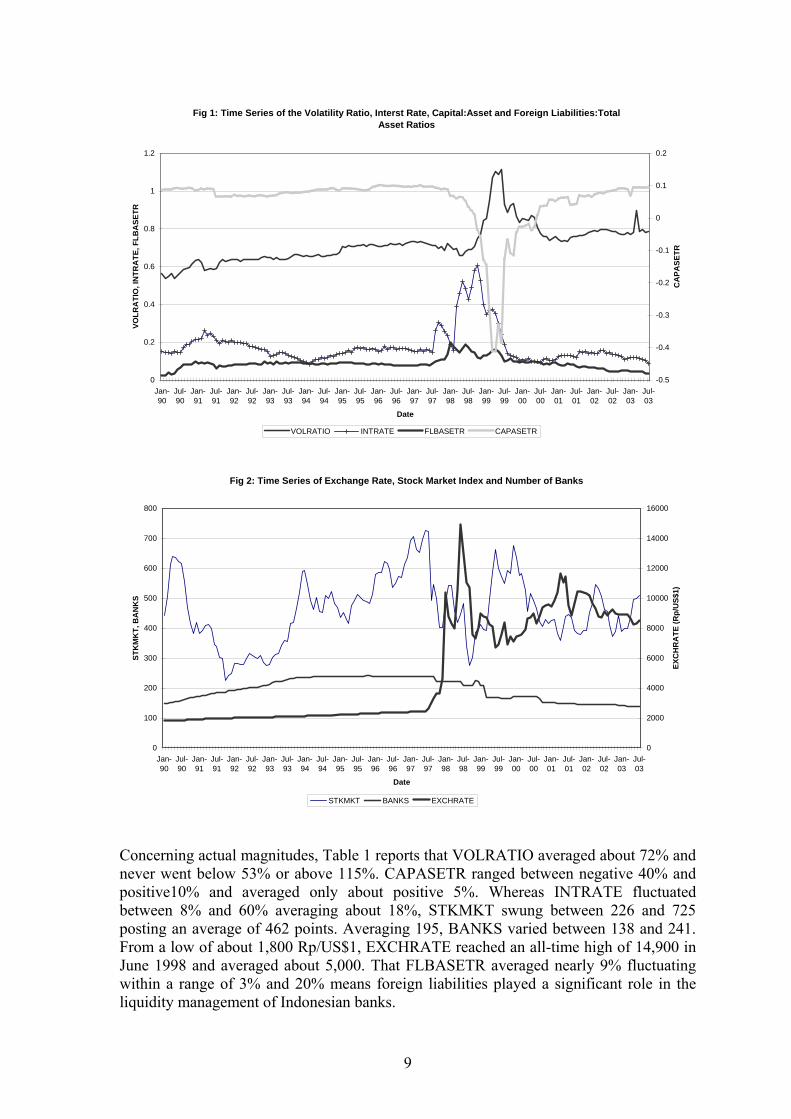
Fig 1: Time Series of the Volatility Ratio, Interst Rate, Capital:Asset and Foreign Liabilities:Total Asset Ratios

0

0.2

0.4

0.6

0.8

1

1.2

Jan-90

Jul-90

Jan-91

Jul-91

Jan-92

Jul-92

Jan-93

Jul-93

Jan-94

Jul-94

Jan-95

Jul-95

Jan-96

Jul-96

Jan-97

Jul-97

Jan-98

Jul-98

Jan-99

Jul-99

Jan-00

Jul-00

Jan-01

Jul-01

Jan-02

Jul-02

Jan-03

Jul-03

Date

VOLR

ATI

O, I

NTR

ATE

, FLB

ASE

TR

-0.5

-0.4

-0.3

-0.2

-0.1

0

0.1

0.2

CA

PASE

TR

VOLRATIO INTRATE FLBASETR CAPASETR

oncerning actual magnitudes, Table 1 reports that VOLRATIO averaged about 72% and

liquidity management of Indonesian banks.

Fig 2: Time Series of Exchange Rate, Stock Market Index and Number of Banks

0

100

200

300

400

500

600

700

800

Jan-90

Jul-90

Jan-91

Jul-91

Jan-92

Jul-92

Jan-93

Jul-93

Jan-94

Jul-94

Jan-95

Jul-95

Jan-96

Jul-96

Jan-97

Jul-97

Jan-98

Jul-98

Jan-99

Jul-99

Jan-00

Jul-00

Jan-01

Jul-01

Jan-02

Jul-02

Jan-03

Jul-03

Date

STK

MK

T, B

AN

KS

0

2000

4000

6000

8000

10000

12000

14000

16000

EXC

HR

ATE

(Rp/

US$

1)

STKMKT BANKS EXCHRATE

Cnever went below 53% or above 115%. CAPASETR ranged between negative 40% and positive10% and averaged only about positive 5%. Whereas INTRATE fluctuated between 8% and 60% averaging about 18%, STKMKT swung between 226 and 725 posting an average of 462 points. Averaging 195, BANKS varied between 138 and 241. From a low of about 1,800 Rp/US$1, EXCHRATE reached an all-time high of 14,900 in June 1998 and averaged about 5,000. That FLBASETR averaged nearly 9% fluctuating within a range of 3% and 20% means foreign liabilities played a significant role in the

9

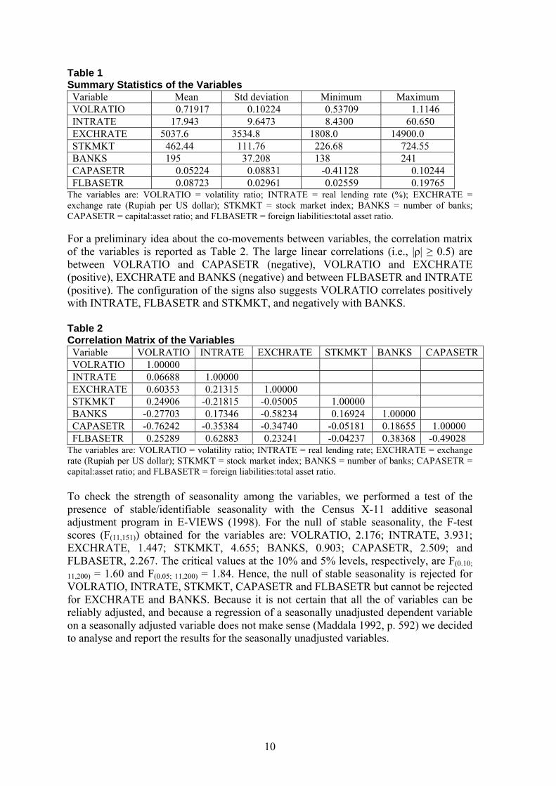
Table 1 Summary Statistics of the Variables Variable Mean Std deviation Minimum Maximum VOLRATIO 0.71917 0.10224 0.53709 1.1146 INTRATE 1 7.943 9.6473 8.4300 60.650 EXCHRATE 503 353 180 14907.6 4.8 8.0 0.0 STKMKT 4 11 22 762.44 1.76 6.68 24.55 BANKS 195 37.208 138 241 CAPASETR 44 0.05224 0.08831 -0.41128 0.102FLBASETR 23 9765 0.087 0.02961 0.02559 0.1

T e: VOLRA ility r TE = g rate (%); TE = e Rupiah per ); STKM ck market ANKS = n ks;

the variables is reported as Table 2. The large linear correlations (i.e., |ρ| ≥ 0.5) are

orrelation Matrix of the Variables VOLRATIO INTRATE EXCHRATE STKMKT BANKS CAPASETR

he variables ar TIO = volat atio; INTRA real lendin EXCHRAxchange rate ( US dollar KT = sto index; B umber of ban

CAPASETR = capital:asset ratio; and FLBASETR = foreign liabilities:total asset ratio. For a preliminary idea about the co-movements between variables, the correlation matrix ofbetween VOLRATIO and CAPASETR (negative), VOLRATIO and EXCHRATE (positive), EXCHRATE and BANKS (negative) and between FLBASETR and INTRATE (positive). The configuration of the signs also suggests VOLRATIO correlates positively with INTRATE, FLBASETR and STKMKT, and negatively with BANKS. Table 2 CVariableVOLRATIO 1.00000 INTRATE 0.06688 1.00000 EXCHRATE 0.60353 0.21315 1.00000 STKMKT 0.24906 -0.21815 -0.05005 1.00000 BANKS -0.27703 0.17346 -0.58234 0.16924 1.00000 CAPASETR 0.18655 1.00000 -0.76242 -0.35384 -0.34740 -0.05181 FLBASETR - -0.49028 0.25289 0.62883 0.23241 0.04237 0.38368

T : V = v io; real ; E r U KM m BANK r A

we performed a test of the resence of stable/identifiable seasonality with the Census X-11 additive seasonal

he variables are OLRATIO olatility rat INTRATE = lending rate XCHRATE = exchangeate (Rupiah per S dollar); ST KT = stock arket index; S = numbe of banks; C PASETR =

capital:asset ratio; and FLBASETR = foreign liabilities:total asset ratio. To check the strength of seasonality among the variables,padjustment program in E-VIEWS (1998). For the null of stable seasonality, the F-test scores (F(11,151)) obtained for the variables are: VOLRATIO, 2.176; INTRATE, 3.931; EXCHRATE, 1.447; STKMKT, 4.655; BANKS, 0.903; CAPASETR, 2.509; and FLBASETR, 2.267. The critical values at the 10% and 5% levels, respectively, are F(0.10;

11,200) = 1.60 and F(0.05; 11,200) = 1.84. Hence, the null of stable seasonality is rejected for VOLRATIO, INTRATE, STKMKT, CAPASETR and FLBASETR but cannot be rejected for EXCHRATE and BANKS. Because it is not certain that all the of variables can be reliably adjusted, and because a regression of a seasonally unadjusted dependent variable on a seasonally adjusted variable does not make sense (Maddala 1992, p. 592) we decided to analyse and report the results for the seasonally unadjusted variables.

10

From the foregoing, therefore, the variables in the empirical model are:

VOLRATIO = volatility ratio (in decimals) LNRIRATE = natural logarithm of the real lending rate LNEXRATE = natural logarithm of the exchange rate Rupiah per US dollar LNSTKMKT = natural logarithm of the Jakarta stock market index LNBANKS = natural logarithm of the number of banks CAPASETR = capital:asset ratio (in decimals) FLBASETR =foreign liabilities:total asset ratio (in decimals)

And the empirical long-run model to be estimated is:

VOLRATIOt = β0 + β1 LNRIRATEt + β2 LNEXRATEt + β3 LNSTKMKTt + β4 LNBANKSt + β5 CAPASETRt + β6 FLBASETRt + et

Estimation Issues The estimation of the regression coefficients employs the MICROFIT ARDL procedure for cointegration. As mentioned earlier, the MICROFIT approach to estimating the ARDL involves firstly the F-test to ascertain that a long-run relationship does exist between the dependent variable and the independent variables. Following that, the short-run coefficients are estimated and out of them the long-run coefficients are calculated. Because monthly data have been used in this study the maximum lag length was set at 12 (Hamilton, 1994, p. 583). The F-test yielded a value of 3.2494 which falls within both the critical value bands of 2.141 and 3.250 (at the 10% level of significance) and 2.476 and 3.646 (at the 5% level of significance), respectively, for the case of 6 regressors with intercept and no trend. Thus, the inference of long-run relationship is inconclusive and depends on whether the underlying variables are I(0) or I(1) or fractionally integrated. To test for the order of integration in the variables the Augmented Dickey Fuller (ADF) and Phillips-Perron (PP) unit root tests were implemented; the results are presented in Table 4. Based on the PP results at the 5% level of significance, all the variables are declared to be I(1)12. Furthermore, to test for cointegration among the variables, the Johansen procedure was applied and the eigenvalue and trace test results are provided in Table 5. Since the first null (of r = 0) is rejected and the second null (of r ≤ 1) is not rejected at the 10% level, it

12 There are some conflicting results from the ADF and PP tests: at both the 10% and 5% levels of significance, ADF declares LNRIRATE to be I(0) but PP declares it to be I(1); ADF declares LNSTKMKT to be I(1) at both the 10% and 5% levels but PP declares it to be I(0) at the 10% level but I(1) at the 5% level. Where there is inconsistency between the ADF and PP results, the conclusion from the PP test is to be preferred because the ADF test is based on the assumption that the series is generated by an autoregressive (AR) process whilst the PP test is based on the more general autoregressive integrated moving average (ARIMA) process (Schwert, 1989; Lin, 1995).

11

is concluded that the variables are cointegrated with one cointegrating vector (or that r = 1). These test results paved the way to apply the ARDL model.13

Table 4 Unit Root Test Results (Sample Period: Jan 1990 – Jul 2003)

Levels First Differences Variable ADF PP ADF PP VOLRATIO -2.0051 -2.0774 -4.1079 -11.545 LNRIRATE -3.1225 -1.8263 -3.0680 -10.580 LNEXRATE -0.9753 -0.8600 -3.9334 -11.190 LNSTKMKT -2.3069 -2.6334 -4.3289 -10.631 LNBANKS -2.1115cwt -2.2175cwt -4.2025cwt -12.598cwt

CAPASETR -2.1610 -2.2874 -3.8884 -10.981 FLBASETR -2.1489 -2.4404 -4.6714 -11.175

All variables are ‘constant, no trend’ except LNBANKS which is ‘constant with trend’ (indicated with superscript ‘cwt’). Critical values for ‘constant, no trend’ = -2.57(10%); -2.90(5%). Critical values for ‘constant with trend’ = -3.13(10%); -3.43(5%) Table 5 The Johansen Cointegration Test Results (Sample Period: Jan 1990 – Jul 2003)

Eigenvalue Null Hypothesis Trace Test p-value 0.45814 r = 0 131.87265 0.08859 0.37142 r ≤ 1 90.81896 0.29341 0.28492 r ≤ 2 59.71095 0.52573 0.19105 r ≤ 3 37.24176 0.60338 0.13979 r ≤ 4 23.03657 0.47616 0.11296 r ≤ 5 12.94796 0.23729 0.07076 r ≤ 6 4.91730 0.02403

4. EMPIRICAL RESULTS AND DISCUSSION Based on the SBC, the optimal ARDL model selected by MICROFIT is ARDL(1, 0, 0, 0, 3, 1, 1). The SBC was preferred because it is more parsimonious than the other popular criterion, the AIC. The empirical results are furnished in Tables 6 - 9. Table 6 gives the results for the empirical ARDL(1, 0, 0, 0, 3, 1, 1) model and contains the short-run coefficients. From the accompanying summary statistics of the R2, the 2R and the F-statistic, the selected ARDL(·) model has a good fit. The model also passes a battery of diagnostic tests indicating there are no serious problems with serial correlation, functional form and heteroskedasticity.

13 The use of the maximum lag length of 12 because of the monthly data means the effective sample period is January 1991 to July 2003. To estimate an ARDL model for m-independent variables and a specified lag length h, MICROFIT needs to run h(h+1)m regressions before choosing the optimal model. In our context where h = 12 and m = 6, the number of regressions to be run is 12(136) = 57,921,708. This is impractical, and indeed no results could be obtained after 9 days continuous running of our PC; apparently MICROFIT simply crashed under such a task. The practical approach taken was to run the model sequentially from lag 12 downward for the same effective period. No results could be obtained for lags 5 or greater. Results for lag 3 were the same as for lag 4 and were an improvement over the results for lags 1 and 2. The results reported and interpreted in the study are those for lag 3. Since the diagnostic test results were favourable it is our contention that these results are plausible and that the potential cost of effecting lag 12 would far outweigh the benefit of getting “more precise” coefficients.

12

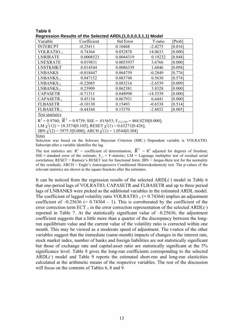
Table 6 Regression Results of the Selected ARDL(1,0,0,0,3,1,1) Model Variable Coefficient Std Error T-ratio [Prob] INTERCPT -0.25411 0.10468 -2.4275 [0.016] VOLRATIO–1 0.74364 0.052878 14.0633 [0.000] LNRIRATE 0.0008523 0.0044319 0.19232 [0.848] LNEXRATE 0.019831 0.0053937 3.6766 [0.000] LNSTKMKT 0.014544 0.0086339 1.6846 [0.094] LNBANKS -0.018447 0.064759 -0.2849 [0.776] LNBANKS-1 0.047152 0.083748 0.5630 [0.574] LNBANKS-2 -0.22085 0.083216 -2.6539 [0.009] LNBANKS-3 0.23909 0.062381 3.8328 [0.000] CAPASETR -0.71311 0.048998 -14.5539 [0.000] CAPASETR-1 0.45134 0.067931 6.6441 [0.000] FLBASETR -0.10130 0.15493 -0.6538 [0.514] FLBASETR-1 -0.44344 0.15370 -2.8852 [0.005] Test statistics R2 = 0.9760; 2R = 0.9739; SSE = .015653; F(12,138) = 468.0230[0.000]; LM χ2(12) = 18.3574[0.105]; RESET χ2(1) = 0.63271[0.426]; JBN χ2(2) = 3975.5[0.000]; ARCH χ2(1) = 1.0544[0.304]

Notes Selection was based on the Schwarz Bayesian Criterion (SBC.) Dependent variable is VOLRATIO. Subscript after a variable identifies the lag. The test statistics are: R2 = coefficient of determination; 2R = R2 adjusted for degrees of freedom; SSE = standard error of the estimate; F(.) = F-statistic; LM = Lagrange multiplier test of residual serial correlation; RESET = Ramsey’s RESET test for functional form; JBN = Jarque-Bera test for the normality of the residuals; ARCH = Engle’s Autoregressive Conditional Heteroskedasticity test. The p-values of the relevant statistics are shown in the square brackets after the estimates. It can be noticed from the regression results of the selected ARDL(·) model in Table 6 that one-period lags of VOLRATIO, CAPASETR and FLBASETR and up to three period lags of LNBANKS were picked as the additional variables in the estimated ARDL model. The coefficient of lagged volatility ratio VOLRATIO–1 (= 0.74364) implies an adjustment coefficient of –0.25636 (= 0.74364 – 1). This is corroborated by the coefficient of the error correction term ECT–1 in the error correction representation of the selected ARDL(·) reported in Table 7. At the statistically significant value of –0.25636, the adjustment coefficient suggests that a little more than a quarter of the discrepancy between the long-run equilibrium value and the current value of the volatility ratio is corrected within one month. This may be viewed as a moderate speed of adjustment. The t-ratios of the other variables suggest that the immediate (same-month) impacts of changes in the interest rate, stock market index, number of banks and foreign liabilities are not statistically significant but those of exchange rate and capital:asset ratio are statistically significant at the 5% significance level. Table 8 gives the long-run coefficients corresponding to the selected ARDL(·) model and Table 9 reports the estimated short-run and long-run elasticities calculated at the arithmetic means of the respective variables. The rest of the discussion will focus on the contents of Tables 6, 8 and 9.

13

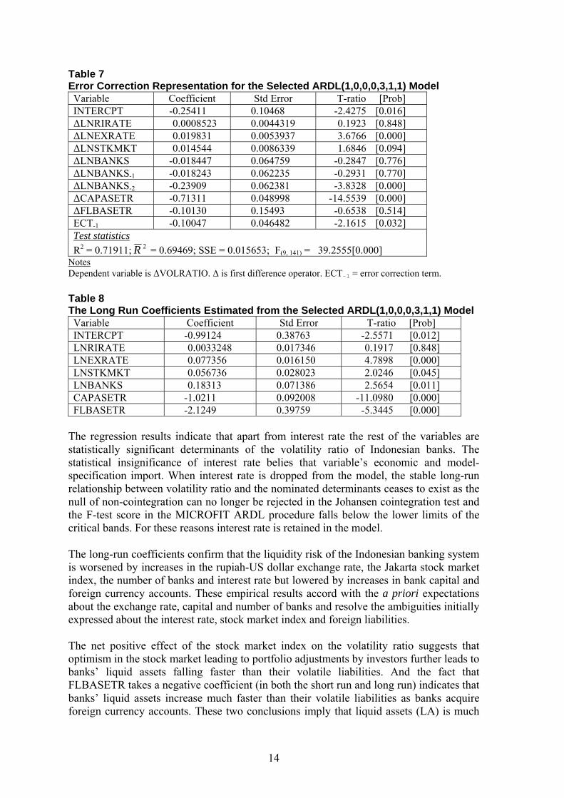
Table 7 Error Correction Representation for the Selected ARDL(1,0,0,0,3,1,1) Model Variable Coefficient Std Error T-ratio [Prob] INTERCPT -0.25411 0.10468 -2.4275 [0.016] ∆LNRIRATE 0.0008523 0.0044319 0.1923 [0.848] ∆LNEXRATE 0.019831 0.0053937 3.6766 [0.000] ∆LNSTKMKT 0.014544 0.0086339 1.6846 [0.094] ∆LNBANKS -0.018447 0.064759 -0.2847 [0.776] ∆LNBANKS-1 -0.018243 0.062235 -0.2931 [0.770] ∆LNBANKS-2 -0.23909 0.062381 -3.8328 [0.000] ∆CAPASETR -0.71311 0.048998 -14.5539 [0.000] ∆FLBASETR -0.10130 0.15493 -0.6538 [0.514] ECT-1 -0.10047 0.046482 -2.1615 [0.032] Test statistics R2 = 0.71911; 2R = 0.69469; SSE = 0.015653; F(9, 141) = 39.2555[0.000]

Notes Dependent variable is ∆VOLRATIO. ∆ is first difference operator. ECT-1 = error correction term. Table 8 The Long Run Coefficients Estimated from the Selected ARDL(1,0,0,0,3,1,1) Model Variable Coefficient Std Error T-ratio [Prob] INTERCPT -0.99124 0.38763 -2.5571 [0.012] LNRIRATE 0.0033248 0.017346 0.1917 [0.848] LNEXRATE 0.077356 0.016150 4.7898 [0.000] LNSTKMKT 0.056736 0.028023 2.0246 [0.045] LNBANKS 0.18313 0.071386 2.5654 [0.011] CAPASETR -1.0211 0.092008 -11.0980 [0.000] FLBASETR -2.1249 0.39759 -5.3445 [0.000]

The regression results indicate that apart from interest rate the rest of the variables are statistically significant determinants of the volatility ratio of Indonesian banks. The statistical insignificance of interest rate belies that variable’s economic and model-specification import. When interest rate is dropped from the model, the stable long-run relationship between volatility ratio and the nominated determinants ceases to exist as the null of non-cointegration can no longer be rejected in the Johansen cointegration test and the F-test score in the MICROFIT ARDL procedure falls below the lower limits of the critical bands. For these reasons interest rate is retained in the model. The long-run coefficients confirm that the liquidity risk of the Indonesian banking system is worsened by increases in the rupiah-US dollar exchange rate, the Jakarta stock market index, the number of banks and interest rate but lowered by increases in bank capital and foreign currency accounts. These empirical results accord with the a priori expectations about the exchange rate, capital and number of banks and resolve the ambiguities initially expressed about the interest rate, stock market index and foreign liabilities. The net positive effect of the stock market index on the volatility ratio suggests that optimism in the stock market leading to portfolio adjustments by investors further leads to banks’ liquid assets falling faster than their volatile liabilities. And the fact that FLBASETR takes a negative coefficient (in both the short run and long run) indicates that banks’ liquid assets increase much faster than their volatile liabilities as banks acquire foreign currency accounts. These two conclusions imply that liquid assets (LA) is much

14

more reactive than volatile liabilities (VL) when the two of them are responding in the same direction to a stimulus. A check of their time series reveals that LA has a coefficient of variation of 1.548 whilst VL has 0.723, underscoring the greater relative variability of LA. Concerning interest rate, it can be inferred from what has just been said about the relative variability of LA and VL that in the context of our model the “deposit effect” is negative and the “stock market effect” is positive. Consequently, the overall positive effect of interest rate implies that the joint positive exchange rate, lending and stock market effects “outweigh” the negative deposit effect. What this helps to clarify is that the policy of increasing interest rate to defend the rupiah has deleterious effect on the FVR and is generally misguided because it is based on the mistaken notion about the expectations formation mechanism that domestic interest rate hikes, relative to foreign interest rates, signal a relative shortage of liquidity in the domestic money market rather than a higher expected domestic inflation rate. After those observations our interpretations of the magnitudes of the estimated multipliers now ensue. Considering first the two variables whose slope coefficients measure the absolute change in VOLRATIO induced by a given absolute change in the value of the respective variable, an increase of one-hundredth of a point (i.e., 0.01 or 1 percentage point) in CAPASETR induces a decrease of 0.007131 (or about 0.71 percentage point) in VOLRATIO in the short run and 0.010211 (or about 1 percentage point) in the long run; a similar increase in FLBASETR induces a decrease of 0.001013 (or about 0.1 percentage point) in VOLRATIO in the short run and 0.021249 (or about 2 percentage points) in the long run. The long-run multipliers for CAPASETR and FLBASETR are, respectively, 1.5 times and 20 times the magnitudes of their short-run counterparts. Among the remaining four variables (whose slope coefficients measure the absolute change in VOLRATIO induced by a relative/percent change in the value of the respective variable) the short-run and long-run coefficients of LNRIRATE, although statistically insignificant, connote that if the interest rate increases by 1%, VOLRATIO would increase by the imperceptible amount of 0.0008523 (or about 0.09 of a percentage point) in the short run and by 0.003248 (or about 0.3 of a percentage point) in the long run. Those for LNEXRATE mean that if the exchange rate depreciates by 1%, VOLRATIO would increase by 0.019831 (or nearly 2 percentage points) in the short run and by 0.077356 (or nearly 8 percentage points) in the long run. Concerning LNSTKMKT the estimated coefficients suggest that 1% increase in the stock market index would induce an increase of 0.014544 (or nearly 1.5 percentage points) in VOLRATIO in the short run and 0.056736 (or nearly 6 percentage points) in the long run. Comparatively, the long-run multipliers of interest rate, the exchange rate and the stock market index are 4 times the sizes of the corresponding short-run estimates. And finally, regarding LNBANKS, if the number of banks increases by 1%, VOLRATIO is expected to decrease immediately by 0.018447 points (or nearly 2 percentage points), fluctuate in the interim period and over the long haul rise by 0.18313 (or about 18 percentage points). Conversely, the reduction in the number of banks (presumably from the closure or liquidation of insolvent ones) impairs the liquidity risk in the short term but engenders improvement in the long term. A noteworthy aspect of the empirical ARDL model is the selection/incorporation of multiple lags of LNBANKS. That the multiplier is negative for the current period and alternates thereafter warrants a comment or two. The negative current-period multiplier of LNBANKS captures the likelihood that the advent of new banks augments total bank capital instantaneously thus lowering the volatility ratio in the same month. Later, after

15

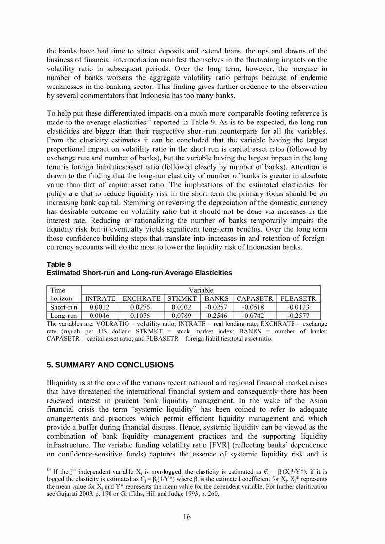
the banks have had time to attract deposits and extend loans, the ups and downs of the business of financial intermediation manifest themselves in the fluctuating impacts on the volatility ratio in subsequent periods. Over the long term, however, the increase in number of banks worsens the aggregate volatility ratio perhaps because of endemic weaknesses in the banking sector. This finding gives further credence to the observation by several commentators that Indonesia has too many banks. To help put these differentiated impacts on a much more comparable footing reference is made to the average elasticities14 reported in Table 9. As is to be expected, the long-run elasticities are bigger than their respective short-run counterparts for all the variables. From the elasticity estimates it can be concluded that the variable having the largest proportional impact on volatility ratio in the short run is capital:asset ratio (followed by exchange rate and number of banks), but the variable having the largest impact in the long term is foreign liabilities:asset ratio (followed closely by number of banks). Attention is drawn to the finding that the long-run elasticity of number of banks is greater in absolute value than that of capital:asset ratio. The implications of the estimated elasticities for policy are that to reduce liquidity risk in the short term the primary focus should be on increasing bank capital. Stemming or reversing the depreciation of the domestic currency has desirable outcome on volatility ratio but it should not be done via increases in the interest rate. Reducing or rationalizing the number of banks temporarily impairs the liquidity risk but it eventually yields significant long-term benefits. Over the long term those confidence-building steps that translate into increases in and retention of foreign-currency accounts will do the most to lower the liquidity risk of Indonesian banks. Table 9 Estimated Short-run and Long-run Average Elasticities

Variable Time horizon INTRATE EXCHRATE STKMKT BANKS CAPASETR FLBASETR Short-run 0.0012 0.0276 0.0202 -0.0257 -0.0518 -0.0123 Long-run 0.0046 0.1076 0.0789 0.2546 -0.0742 -0.2577

The variables are: VOLRATIO = volatility ratio; INTRATE = real lending rate; EXCHRATE = exchange rate (rupiah per US dollar); STKMKT = stock market index; BANKS = number of banks; CAPASETR = capital:asset ratio; and FLBASETR = foreign liabilities:total asset ratio. 5. SUMMARY AND CONCLUSIONS Illiquidity is at the core of the various recent national and regional financial market crises that have threatened the international financial system and consequently there has been renewed interest in prudent bank liquidity management. In the wake of the Asian financial crisis the term “systemic liquidity” has been coined to refer to adequate arrangements and practices which permit efficient liquidity management and which provide a buffer during financial distress. Hence, systemic liquidity can be viewed as the combination of bank liquidity management practices and the supporting liquidity infrastructure. The variable funding volatility ratio [FVR] (reflecting banks’ dependence on confidence-sensitive funds) captures the essence of systemic liquidity risk and is 14 If the jth independent variable Xj is non-logged, the elasticity is estimated as Єj = βj(Xj*/Y*); if it is logged the elasticity is estimated as Єj = βj(1/Y*) where βj is the estimated coefficient for Xj, Xj* represents the mean value for Xj and Y* represents the mean value for the dependent variable. For further clarification see Gujarati 2003, p. 190 or Griffiths, Hill and Judge 1993, p. 260.

16

logically closely linked to the factors that affect a balanced liquidity infrastructure: the design of prudential and monetary instruments, existence of legal contract rights and the efficiency of the court system, foreign exchange regulations, variability of interest rates, exchange rates and safety-net provisions. Hitherto, the research practice has been to interpret estimated FVRs against the backdrop of the characteristics of the liquidity infrastructure. This study set out to quantify the relationship between FVR and the measurable determinants of a balanced liquidity infrastructure in a dynamic framework for Indonesia, the country worst affected by the Asian crisis of 1997/98. Monthly data covering the period January 1990 to July 2003 were analysed employing the MICROFIT ARDL (autoregressive distributed lag) approach to cointegration that effects the recommended simultaneous estimation of the short-run and long-run coefficients in a dynamic regression model. A good fit and favourable diagnostic test results were obtained for the model that yielded credible estimates of the short-run and long-run multipliers and elasticities. The regression results show that FVR is increasing in exchange rate, the Jakarta stock market index, interest rate and the number of banks, and decreasing in capital:asset ratio and foreign liabilities:total asset ratio. To reduce the FVR in the short term the best option lies with increasing bank capital. Over the long term enduring increases in foreign-currency accounts and reduction in the number of banks seem to hold the greatest prospects for lowering the FVR.

17

18

REFERENCES Banerjee, A., Dolado, J. J., Hendry D. F. and Smith, G. W. (1986). Exploring equilibrium

relationships in econometrics through static models: Some Monte Carlo evidence, Oxford Bulletin of Economics and Statistics, 48, 253-278.

Banerjee, A., Dolado, J. J., Galbraith, J. W. and Hendry D. F. (1993). Co-integration, error correction and the econometric analysis of non-stationary data. Oxford University Press: Oxford.

Bank Indonesia. Statistik ekonomi dan keuangan Indonesia (The Indonesian Economic and Financial Statistics), various issues. Jakarta, Indonesia.

Barnett, W. and Liu, Y. (1995). The CAMP – Extended divisia monetary aggregate with exact tracking under risk (Working Paper No. 195). University of Washington, Department of Economics: St. Louis.

Berg, A. and Patillo, C. (1999). Are currency crises predictable? A test, IMF Staff Papers, 40(2), 107-138.

Bewley, R. (1979). The direct estimation of the equilibrium response in a linear dynamic model, Economic Letters, 3, 357-361.

Coe, D. T. and Helpman, E. (1995). International R & D spillovers, European Economic Review, 39, 859-887.

Cole, D. C. and Slade, B. F. (1998). Why has Indonesia’s financial crisis been so bad? Bulletin of Indonesian Economic Studies, 34(2), 61-66.

Corsetti, G., Pesenti, P. and Roubini, N. (1998a). Paper tigers? A model of the Asian crisis (NBER Working Paper No. 6783). National Bureau of Economic Research: Cambridge, MA.

Corsetti, G., Pesenti, P. and Roubini, N. (1998b). What caused the Asian currency and financial crises? Part I: A macroeconomic overview (NBER Working Paper No. 6833). National Bureau of Economic Research: Cambridge, MA.

Corsetti, G., Pesenti, P. and Roubini, N. (1998c). What caused the Asian currency and financial crises? Part II The policy debate (NBER Working Paper No. 6834). National Bureau of Economic Research: Cambridge, MA.

Djiwandono, S. (2001). Mengelola Bank Indonesia dalam masa krisi (Managing Bank Indonesia in the crisis period) (LP3ES). Jakarta.

Drake, L. and Chrystal, K. A. (1997). Personal sector money demand in the UK, Oxford Economic Papers, 49(2), 188-206.

Dziobek, C., Hobbs, J. K. and Marston, D. (2000). Toward a framework for systemic liquidity policy (IMF Working Paper No. WP/00/34). International Monetary Fund: Washington DC.

Dziobek, C., Hobbs, J. K. and Marston, D. (2002). Toward a framework for systemic liquidity policy, in Enoch, C. et al. (Eds.). Building Strong Banks Through Surveillance and Resolution. International Monetary Fund: Washington DC.

Eichengreen, B., Rose, A. K. and Wyplosz, C. (1995). Exchange market mayhem: The antecedents and aftermath of speculative attacks, Economic Policy, 21, 249-312.

Engle, R. F. and Granger, C. W. J. (1987). Cointegration and error correction: Representations, estimation and testing, Econometrica, 55, 252-276.

Enoch, C., Taylor, M. W. and Marston, D. (Eds.). (2002). Building strong banks through surveillance and resolution. International Monetary Fund: Washington DC.

E-Views. (1998). Quantitative Micro Software, Irvine, CA. Frankel, J. A. and Rose, A. K. (1996). Currency crashes in emerging markets: An

empirical treatment, Journal of International Economics, 41, 351-366.

19

Furman, J. and Stiglitz, J. E. (1998). Economic crisis: Evidence and insights from East Asia, Brookings Papers on Economic Activity, 2, 1-135.

Griffiths, W. E., Hill, R. C. and Judge, G. G. (1993). Learning and practicing econometrics. John Wiley and Sons: New York.

Group of 22. (1998). Report of the working group on strengthening financial systems, G-22. Washington DC.

Gujarati, D. N. (2003). Basic econometrics (4th ed.). McGraw-Hill: New York. Hamilton J. D. (1994). Time series analysis. Princeton University Press: Princeton, NJ. Harvey, A. C. (1993). Time series models (2nd ed.). Harvester Wheatsheaf: Hemel

Hempstead, UK. Hendry, D. F. (1995). Dynamic econometrics. Oxford University Press: Oxford. Kaminsky, G. L., Lizondo, S. and Reinhart, C. M. (1998). Leading indicators of currency

crises, IMF Staff Papers, 45(1), 1-48. Kaminsky, G. L. and Reinhart, C. M. (1998). Financial crises in Asia and Latin America:

Then and now, American Economic Review, 88(2), 444-448. Kaminsky, G. L. and Reinhart, C. M. (1999). The twin crises: The causes of banking and

balance of payments problems, American Economic Review, 89(3), 473-500. Keller, C., Rosenberg, C., Roubini, N. and Setser, B. (2002). The bottom line, Finance

and Development, December. International Monetary Fund: Washington DC. Lin, C. A. (1995). More evidence on Wagner’s Law for Mexico, Public Finance, 50(2),

267-277. Maddala, G. S. (1992). Introduction to econometrics (2nd ed.). Macmillan Publishing Co:

New York. Maddala, G. S. and Kim, In-Moo. (1998). Unit roots, cointegration and structural

change. Cambridge University Press: Cambridge. Mishkin, F. S. (1998). The economics of money, banking and financial markets (5th ed.).

Addison Wesley Longman: Reading, MA. Montes, M. F. (1998). The currency crisis in Southeast Asia (Updated ed.). Institute of

Southeast Asian Studies: Singapore. Moosa, I. A. (2000). Exchange rate forecasting: Techniques and applications. Macmillan

Press: London. Nasution, A. (1999). The financial crisis in Indonesia, in Seiichi Masuyama, Donna

Vandenbrink and Chia Siow Yue (Eds.). East Asia’s Financial Systems: Evolution and Crisis. Nomura Research Institute and Institute of Southeast Asian Studies: Tokyo.

Pangestu, M. and Habir, M. (2002a). The boom, bust and restructuring of Indonesian banks (IMF Working Paper No. 02/66). International Monetary Fund: Washington DC.

Pangestu, M. and Habir, M. (2002b). Restructuring of Indonesian banks post 1997-1998 crisis, www.adbi.org/publications/dp/PangestuandHabir3b.pdf.

Patterson, K. (2000). An introduction to applied econometrics: A time series approach. Macmillan Press: London.

Pesaran, H. M. and Shin, Y. (1995). An autoregressive distributed lag modelling approach to cointegration analysis (DAE Working Paper Series, No. 9514). University of Cambridge, Department of Applied Economics: Cambridge.

Pesaran, H. M., Shin, Y. and Smith, R. (1996). Testing the existence of a long-run relationship (DAE Working Paper Series, No. 9622) University of Cambridge, Department of Applied Economics: Cambridge.

Pesaran, H. M. and Pesaran, B. (1997). Microfit 4.0. Oxford University Press: Oxford.

20

Radelet, S. and Sachs, J. D. (1998). The onset of the East Asian financial crisis (NBER Working Paper No. 6680) National Bureau of Economic Research: Cambridge, MA.

Sachs, J. D., Tornell, A. and Velasco, A. (1996). The Mexican peso crisis: Sudden death or death foretold? Journal of International Economics, 41, 265-283.

Schwert, G. W. (1989) Tests for unit roots: A Monte Carlo investigation, Journal of Business and Economic Statistics, 7, 147-159.

Wickens, M. R. and Breusch, T. S. (1988). Dynamic specification, the long-run and the estimation of transformed regression models, Economic Journal, 98, 189-205.

World Bank Policy Research Report. (2001). Finance for growth, policy choices in a volatile world. Oxford University Press: New York.

21

22

LIST OF RECENT DISCUSSION PAPERS 02.01 S. Chatterjee and N. Podder, Equity, efficiency and social welfare: An

application of generalized Lorenz dominance to New Zealand incomes data 1984-98, January 2002.

02.02 S. Richardson, Revisiting the income and growth effects of professional sport

franchises: Does success matter?, January 2002. 02.03 N. Campbell and J. Jude Kline, Do profit maximizers take cold showers?,

January 2002. 02.04 L. M. Smith, A teacher reflects on the introductory economics course and

Samuelson’s Economics, March 2002. 02.05 S. Richardson, Efficiency estimation using the stochastic production frontier

approach: Evidence from the National Rugby League, March 2002. 02.06 S. Chatterjee and N. Podder, Economic inequality in colour: Some ethnic

dimensions of income distribution in New Zealand 1984-98, March 2002. 02.07 J. Obben, Towards a formal profiling model to foster active labour market

policies in New Zealand, April 2002. 02.08 M. E. Ali, Transfer of sustainable energy technology to developing countries as

a means of reducing greenhouse gas emission - The case of Bangladesh: Review of relevant literature, August 2002.

02.09 M. E. Ali, Transfer of sustainable energy technology for rural Bangladesh: Opportunity for New Zealand, August 2002.

02.10 M. E. Ali, Energy consumption pattern in rural Bangladesh - The opportunity for New Zealand: A household survey, October 2002.

02.11 S. Shakur, A. N. Rae and S. Chatterjee, How comprehensive will be the doha

round? Experiments with agricultural and non-agricultural reforms, October 2002.

02.12 J. J. Su, On the size of a serial correlation robust panel unit root test in

cointegrated panels, November 2002. 03.01 J. E. Alvey, Adam Smith’s optimistic teleological view of history, February 2003. 03.02 J. E. Alvey, Adam Smith’s view of history: Consistent or paradoxical?,

March 2003.

23

03.03 H. -J. Engelbrecht and A. Mahon, Maori and the information workforce, 1991-

2001, April 2003.

03.04 J. J. Su, A note on spurious regression in panels with cross-section dependence,

June 2003. 03.05 J. E. Alvey, Adam Smith’s pessimistic view of the future of commercial society:

rhetoric or reality? September 2003. 03.06 J. E. Alvey, Adam Smith’s globalization (but anti-secularization) theory,

September 2003. 03.07 J. Obben and A. E. Nugroho, Determinants of the funding volatility of Indonesian

banks: A dynamic model, December 2003.

24