Detecting Anonymous Target and Predicting Target ... - MDPI

symmetryS S

Article

Detecting Anonymous Target and Predicting Target Trajectoriesin Wireless Sensor Networks

P. Leela Rani 1,* and G. A. Sathish Kumar 2

�����������������

Citation: Leela Rani, P.; Sathish

Kumar, G.A. Detecting Anonymous

Target and Predicting Target

Trajectories in Wireless Sensor

Networks. Symmetry 2021, 13, 719.

https://doi.org/10.3390/sym13040719

Academic Editor: Raúl

Baños Navarro

Received: 4 March 2021

Accepted: 15 April 2021

Published: 19 April 2021

Publisher’s Note: MDPI stays neutral

with regard to jurisdictional claims in

published maps and institutional affil-

iations.

Copyright: © 2021 by the authors.

Licensee MDPI, Basel, Switzerland.

This article is an open access article

distributed under the terms and

conditions of the Creative Commons

Attribution (CC BY) license (https://

creativecommons.org/licenses/by/

4.0/).

1 Department of Information Technology, Sri Venkateswara College of Engineering, Pennalur Village,Chennai-Bengaluru High Road, Sriperumbudur Tk., Kancheepuram Dist., Chennai 602117, India

2 Department of Electronics & Communication Engineering, Sri Venkateswara College of Engineering,Pennalur Village, Chennai-Bengaluru High Road, Sriperumbudur Tk., Kancheepuram Dist.,Chennai 602117, India; [email protected]

* Correspondence: [email protected]

Abstract: Target Tracking (TT) is an application of Wireless Sensor Networks (WSNs) which neces-sitates constant assessment of the location of a target. Any change in position of a target and thedistance from each intermediate sensor node to the target is passed on to base station and thesefactors play a crucial role in further processing. The drawback of WSN is that it is prone to numerousconstraints like low power, faulty sensors, environmental noises, etc. The target should be detectedfirst and its path should be tracked continuously as it moves around the sensing region. This problemof detecting and tracking a target should be conducted with maximum accuracy and minimumenergy consumption in each sensor node. In this paper, we propose a Target Detection and TargetTracking (TDTT) model for continuously tracking the target. This model uses prelocalization-basedKalman Filter (KF) for target detection and clique-based estimation for tracking the target trajectories.We evaluated our model by calculating the probability of detecting a target based on distance, thenestimating the trajectory. We analyzed the maximum error in position estimation based on densityand sensing radius of the sensors. The results were found to be encouraging. The proposed KF-basedtarget detection and clique-based target tracking reduce overall expenditure of energy, thereby in-creasing network lifetime. This approach is also compared with Dynamic Object Tracking (DOT) andface-based tracking approach. The experimental results prove that employing TDTT improves energyefficiency and extends the lifetime of the network, without compromising the accuracy of tracking.

Keywords: wireless sensor networks; Kalman filter; target detection; target tracking; clique-basedestimation

1. Introduction

TT is a primary and most demanding application of sensor networks that aims todevelop models to determine crucial information about the mobility factors, such as thelocation, velocity, and track of a target [1]. In WSNs, the targets in target tracking algorithmsmay be in active or passive modes. In active mode, the target is active and forms a part ofthe employed model, whereas in passive mode the target has no active part in the trackingfunctionality. This research work concentrates on active target tracking.

The main objective of target tracking is to locate a target and monitor the movementof that target continuously as shown in Figure 1. This may be done with the help of sensorsdeployed in the sensing environment. The sensors may be placed in the environment,randomly or uniformly, depending on the requirement of the application. This targettracking concept is used in myriad of applications such as agriculture, security, smarthomes, and so on. WSN consists of a number of sensor nodes placed in the monitoringarea. The sensor nodes are small with low-power sensing unit. There is also a low-cost, low-capacity battery to make the components work. In target tracking, the targetsmay be positioned statically or may be mobile. The assumption that the position of a

Symmetry 2021, 13, 719. https://doi.org/10.3390/sym13040719 https://www.mdpi.com/journal/symmetry

Symmetry 2021, 13, 719 2 of 22

target is known apriori [2] drives the algorithms in TT to estimate localized position andpath of target using several measurements of target’s transmissions. The metrics thatare gaining importance in this application of WSN are Angle of Arrival (AOA), ReceivedSignal Strength Indication (RSSI) [3], Time-Of-Arrival (TOA) and Time Difference of Arrival(TDOA). The techniques that are RSSI-based have been broadly researched and have gainedpopularity in recent years as they are widely available in wireless devices and extra sensorsare not needed. Target tracking algorithm is divided into target detection, localization,and trajectory estimation [4].Active target tracking algorithms give more importance tolocalization and estimation of paths of a target [5].To deal with the localization problem,various features, viz. TOA, Direction of Arrival (DOA), and RSSI are suggested. Authorsof [6,7] exploit the features of RSSI to track targets.

Symmetry 2021, 13, x FOR PEER REVIEW 2 of 23

low-cost, low-capacity battery to make the components work. In target tracking, the tar-gets may be positioned statically or may be mobile. The assumption that the position of a target is known apriori [2] drives the algorithms in TT to estimate localized position and path of target using several measurements of target’s transmissions. The metrics that are gaining importance in this application of WSN are Angle of Arrival (AOA), Received Signal Strength Indication (RSSI) [3], Time-Of-Arrival (TOA) and Time Difference of Ar-rival (TDOA). The techniques that are RSSI-based have been broadly researched and have gained popularity in recent years as they are widely available in wireless devices and extra sensors are not needed. Target tracking algorithm is divided into target detec-tion, localization, and trajectory estimation [4].Active target tracking algorithms give more importance to localization and estimation of paths of a target [5].To deal with the localization problem, various features, viz. TOA, Direction of Arrival (DOA), and RSSI are suggested. Authors of [6,7] exploit the features of RSSI to track targets.

Figure 1. Target tracking in sensing region.

The propagation path-loss model is normally used to perform localization of the target, which in turn enables target tracking algorithms to deduce the position of the target. The assumptions made in the path-loss model are that the channel is an ideal free-space medium, or channel measurements are done extensively. Nevertheless, envi-ronmental factors, such as attenuation, multipath propagation, and Non-Line-Of-Sight (NLOS) add more complexity to the challenges of TT algorithms [8]. Owing to all these external factors, TT based on RSSI is infeasible in various applications, and requires a thorough list of measurements of channel [9]. Extensive research has been carried out by researchers around the world, focusing on all the external factors in path-loss models. However, the demerit of these approaches is that the models performed reasonably well only in very limited practical scenarios [10]. If these demerits are mitigated, then WSNs can be effectively used for localization and TT.

Apart from WSN, Global Positioning System (GPS) and Bluetooth can be used as required in various applications [11–13]. However, they are not considered to be an op-timal solution due to incurred cost in installing additional receivers to track the targets, interferences, and limited coverage.

This paper focuses on reducing the level of energy consumption and increasing the accuracy of tracking using combined KF and clique-based approach. This TDTT model is fed with RSSI values as input and output in the relevant location of the target. As the target moves along a trajectory, clique-based approach for target tracking senses the di-rection and acceleration of the target and reports the new location of the target in a con-tinuous manner.

The main contributions of this paper include the following:

Figure 1. Target tracking in sensing region.

The propagation path-loss model is normally used to perform localization of thetarget, which in turn enables target tracking algorithms to deduce the position of the target.The assumptions made in the path-loss model are that the channel is an ideal free-spacemedium, or channel measurements are done extensively. Nevertheless, environmentalfactors, such as attenuation, multipath propagation, and Non-Line-Of-Sight (NLOS) addmore complexity to the challenges of TT algorithms [8]. Owing to all these external factors,TT based on RSSI is infeasible in various applications, and requires a thorough list ofmeasurements of channel [9]. Extensive research has been carried out by researchersaround the world, focusing on all the external factors in path-loss models. However,the demerit of these approaches is that the models performed reasonably well only invery limited practical scenarios [10]. If these demerits are mitigated, then WSNs can beeffectively used for localization and TT.

Apart from WSN, Global Positioning System (GPS) and Bluetooth can be used asrequired in various applications [11–13]. However, they are not considered to be anoptimal solution due to incurred cost in installing additional receivers to track the targets,interferences, and limited coverage.

This paper focuses on reducing the level of energy consumption and increasing theaccuracy of tracking using combined KF and clique-based approach. This TDTT model isfed with RSSI values as input and output in the relevant location of the target. As the targetmoves along a trajectory, clique-based approach for target tracking senses the direction andacceleration of the target and reports the new location of the target in a continuous manner.

The main contributions of this paper include the following:(1) TDTT model that uses prelocalization-based KF for target detection and a clique-

based TT methodology; (2) performance evaluation of TDTT via simulations; (3) com-parison of TDTT to DOT and FaceTrack; (4) comparison of TDTT to KF, EKF, DOT, andFaceTrack in terms of accuracy.

In this paper, Section 2 explains related work, Section 3 describes WSN model usedin our proposed system, Section 4 elaborates our proposed architecture and results of ourapproach are presented in Section 5.

Symmetry 2021, 13, 719 3 of 22

2. Related Work

A framework to deal with locating people, finding out their positions, counting people,and tracking their movements was described by Patwari et al. [14]. They also exploitedthe property of penetrating buildings using radio waves for surveillance [15]. Touvat et al.proposed an RSSI-based trilateration approach to compare ISM868 and Zigbee techniqueand used path-loss model to map RSSI to distance [16]. However, this did not producedesirable results when used for localization. Bosisio suggested different frequencies forcalculating RSSI values for the same distance. These RSSI values were then used to increasethe accuracy of the determined distance [17]. This accurate measurement of distance isa crucial factor to achieve an ideal localization and to track the targets more accurately.In [18], various TT techniques based on structure of network were discussed at length.

Accuracy is increased by comparing different RSSI values, as enhanced RSSI accuracyleads to increased accuracy in localization and trajectory estimation [19]. Ceylan et al.suggested different frequencies for measuring RSSI [20]. The same distance was used alongwith different frequencies to measure different RSSI value. A location detection methodemploying learning methods was explained by Hanen Ahmadi et al. [21]. They employeda group of regression trees to accurately track the location of a target. The regressiontrees were formed by capturing the association between RSSI and location of anchor node.RSSI-based localization and techniques to improve accuracy were discussed in detail byS.R. Jondhale [22].

Din et al. [23] presented a clustering-based mating method for direct as well asmultihop routing to increase the network lifetime in WSN. Sthapit, P et al. [24] suggestedusing support vector machine and logistic regression to compute the position. Thenmaximum and minimum error in position estimation were calculated and tabulated. Theaverage error was found to be 50 cm. Banihashemian suggested a range-free localizationtechnique using neural networks and included the concept of Particle Swarm Optimization(PSO) algorithm for optimization [25].

Conventionally, KF [26] is used for tracking a random target. However, KF is con-strained to linear and Gaussian assumptions. Thus, linear measurement model is assumedif KF is to be used for tracking in WSNs. However, real-time target motion is nonlinear, soderivatives of KF like Extended Kalman Filter (EKF) and Unscented Kalman Filter (UKF)are used [27]. In all derivatives of KF, after the nonlinear state is made linear, KF is applied.It is always encouraged to use KF for assessing performance in comparisons.

Fayazi et al. combined Generalized Extended Kalman Filter and Genetic Algorithm II,resulting in reduced energy usage and precise position accuracy [28]. In 2019, S.R. Jondhaleproposed a framework using two algorithms, Generalized Regression Neural Network(GRNN) KF and GRNN + UKF, to estimate the location of a target in motion [29].The abovemethod is implemented in isotropic and anisotropic networks and the results showed thatit resulted in low localization error rate. A localization scheme based on neural networkis portrayed by Po-Jen Chuang that used online training and correlated data to calculateinternode distance [30]. This scheme increased localization success rate and in turn resultedin low error rate.

A location fingerprinting database composed of Wi-Fi, RSSI, and geomagnetic fieldintensity calculated with many devices at a multistory building is presented in [31]. Lo-calization and trajectory inference with Convolutional Neural Network (CNN) and LongShort-Term Memory (LSTM) network was carried out on this database.

It is possible to locate a target using solitary node but this approach results in depletionof energy and enforces more computation load on that particular node. Multiple sensorsserve to reduce load on a particular node and hence, energy depletion will be much loweras the nodes cooperate with each other in tracking the target. This collaboration amongmultiple sensors is mandatory to increase accuracy factor and to decrease energy usage [32].

DOT [33] approach is used to track mobile targets accurately and convey the locationof target to mobile user. This approach does not need frequent queries regarding targetlocation as it uses spatial information stored by neighboring nodes to track a moving target

Symmetry 2021, 13, 719 4 of 22

and thus reduces energy consumption. FaceTrack [34] is a target tracking framework whichis used to construct faces, using the nodes of a spatial region surrounding a target. A targettracking algorithm based on clique, for binary proximity sensor networks, is presented byJaved et al. [35]. This work formed cliques consisting of sensors and achieved less locationerror in TT.

By analyzing the outcome of all the above related work, it is evident that the followingfactors affect the accuracy of target tracking functionality in WSN: faulty sensor nodeslosing targets, delays in TT, usage of energy, connectivity, aggregation, and so on. Asensor node may become faulty due to common scenarios, namely, depletion of battery,environmental disasters, and failure of hardware. The factor that affects the performanceof TT functionality is missing the targets. Targets may be missed due to barriers in thepath of target or due to errors made in prediction of trajectory of the target. All effortsmade to track targets should be concentrated on minimizing the probability of losing thetargets. The next factor in TT is minimizing the delay incurred while tracking the object.The tradeoff between delay and accuracy of tracking algorithm should not be compromised.The essential feature is that the delay is to be reduced while the accuracy of target trackingshould be maintained considerably. Another consideration in tracking is the executiontime of the algorithm. If the algorithm takes longer than expected duration, then the targetwould have relocated to some other position. Coverage refers to number of sensors thatare deployed in the sensing area. Coverage directly affects the performance of WSN. Whencoverage is more, accuracy is considerably improved. This limiting factor necessitatesenergy efficient, adaptive target detection and tracking methodology.

We propose a system that uses KF-based target detection and clique-based targettracking to address the problem of coverage, accuracy, and energy efficiency.

3. WSN Model for Anonymous Target Tracking

In this section, we describe the representation of the entire wireless sensor network,representation of sensors in various modes, energy levels, and target trajectories.

3.1. Rudimentary WSN Representation

A wireless sensor network with ‘M’ nodes is put into operation, for ‘T’ duration, inthe designated sensing area. A target is assumed to be in motion in the sensing area. Anassumption made in this scenario is that sensors deployed in the area belong to the kindof binary sensors that have a prefixed range for sensing. The sensing range of this kindof binary sensor is denoted as ‘R’. The implication of binary sensor is that it returns ‘1’ ifthe object to be tracked is present in the sensing range and returns ‘0’ if the object is out ofrange of the sensing node. This basic model allows computation of the target’s location byobtaining the centroids of reported positions of all sensors within the sensing area at anyinstant ‘t’. Consider ‘m’ sensors are deployed in ‘Yt’ locations. Yt = (xj, yj), where j = 1...m.These ‘m’ sensors are responsible for detecting the target within the sensing range R. Thefuture position is estimated using Equation (1).

Yc(t) = (xc(t), yc (t)) (1)

where xc(t) =∑m xj

m ; yc(t) =∑m yj

m .

3.2. Sensor Representation for Detecting Targets

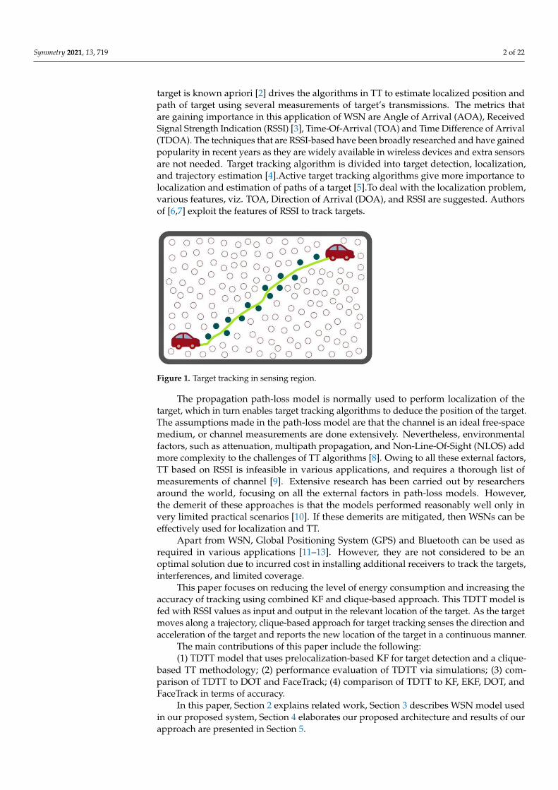
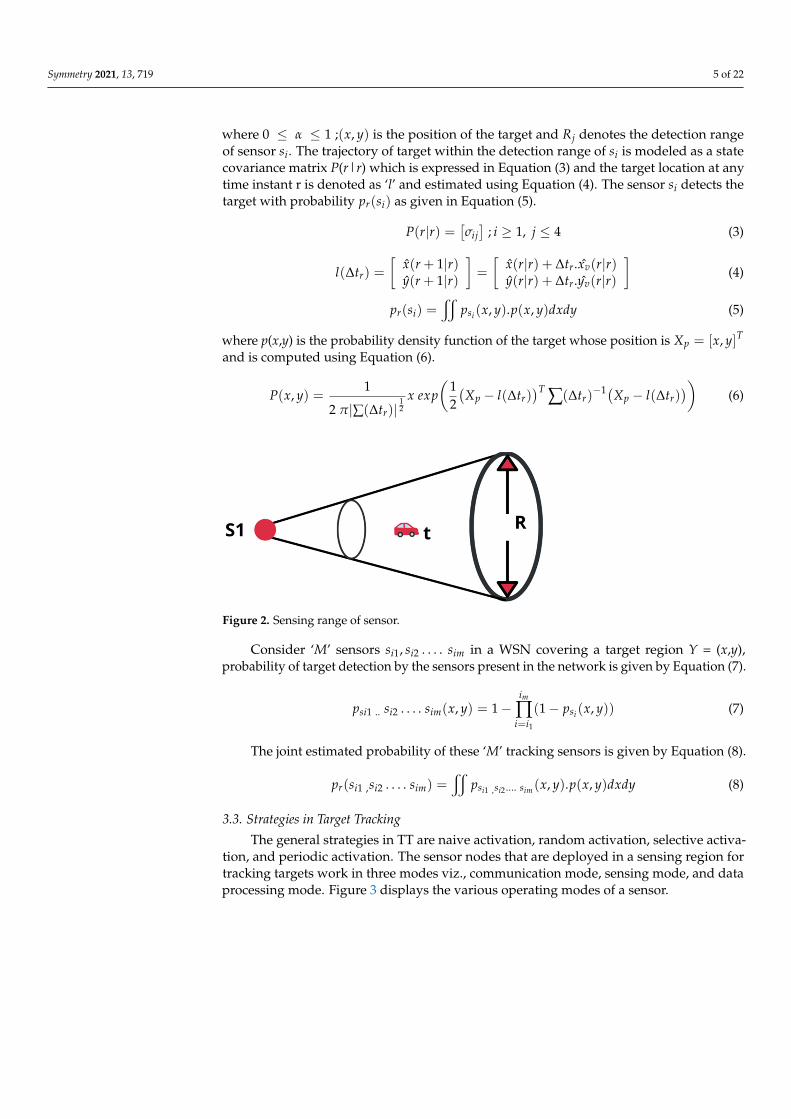
The basic model works perfectly only if target ‘t’ is within the sensing range ‘R’ of asensor as depicted in Figure 2. This assumption does not hold well in real-life scenarios.The target may not always be in detection range of sensors. It is necessary to revise thebasic model to include probability of detection of target by a sensor. The mathematicalmodel of this idea is given in Equation (2).

psi (x, y) ={

α , i f (x, y)εRj0, otherwise

(2)

Symmetry 2021, 13, 719 5 of 22

where 0 ≤ α ≤ 1 ;(x, y) is the position of the target and Rj denotes the detection rangeof sensor si. The trajectory of target within the detection range of si is modeled as a statecovariance matrix P(r|r) which is expressed in Equation (3) and the target location at anytime instant r is denoted as ‘l’ and estimated using Equation (4). The sensor si detects thetarget with probability pr(si) as given in Equation (5).

P(r|r) =[σij]

; i ≥ 1, j ≤ 4 (3)

l(∆tr) =

[x(r + 1|r)y(r + 1|r)

]=

[x(r|r) + ∆tr.xv(r|r)y(r|r) + ∆tr.yv(r|r)

](4)

pr(si) =x

psi (x, y).p(x, y)dxdy (5)

where p(x,y) is the probability density function of the target whose position is Xp = [x, y]T

and is computed using Equation (6).

P(x, y) =1

2 π|∑(∆tr)|12

x exp(

12(Xp − l(∆tr)

)T ∑(∆tr)−1(Xp − l(∆tr)

))(6)

Symmetry 2021, 13, x FOR PEER REVIEW 5 of 23

𝑌 (𝑡) = (𝑥 (𝑡), 𝑦 (𝑡)) (1)

where 𝑥 (𝑡) = ∑; 𝑦 (𝑡) = ∑

.

3.2. Sensor Representation for Detecting Targets The basic model works perfectly only if target ‘t’ is within the sensing range ‘R’ of a

sensor as depicted in Figure 2. This assumption does not hold well in real-life scenarios. The target may not always be in detection range of sensors. It is necessary to revise the basic model to include probability of detection of target by a sensor. The mathematical model of this idea is given in Equation (2).

Figure 2. Sensing range of sensor.

𝑝 (𝑥, 𝑦) = 𝛼 , 𝑖𝑓(𝑥, 𝑦)𝜖𝑅0, 𝑜𝑡ℎ𝑒𝑟𝑤𝑖𝑠𝑒 (2)

where 0 𝛼 1 ;(𝑥, 𝑦) is the position of the target and 𝑅 denotes the detection range of sensor 𝑠 .The trajectory of target within the detection range of 𝑠 is modeled as a state covariance matrix P(r|r) which is expressed in Equation (3) and the target location at any time instant r is denoted as ‘l’ and estimated using Equation (4). The sensor 𝑠 detects the target with probability 𝑝 (𝑠 ) as given in Equation (5). 𝑃(𝑟|𝑟) = 𝜎 ; 𝑖 ≥ 1, 𝑗 4 (3)𝑙(∆𝑡 ) = 𝑥(𝑟 + 1|𝑟)𝑦(𝑟 + 1|𝑟) = 𝑥(𝑟|𝑟) + ∆𝑡 . 𝑥 (𝑟|𝑟)𝑦(𝑟|𝑟) + ∆𝑡 . 𝑦 (𝑟|𝑟) (4)

𝑝 (𝑠 ) = 𝑝 (𝑥, 𝑦). 𝑝(𝑥, 𝑦)𝑑𝑥𝑑𝑦 (5)

where p(x,y) is the probability density function of the target whose position is 𝑋 = 𝑥, 𝑦 and is computed using Equation (6). 𝑃(𝑥, 𝑦) = 12 𝜋|∑(∆𝑡 )| x exp 12 𝑋 − 𝑙(∆𝑡 ) (∆𝑡 ) 𝑋 − 𝑙(∆𝑡 ) (6)

Consider ‘M’ sensors 𝑠 , 𝑠 … . 𝑠 in a WSN covering a target region Y = (x,y), probability of target detection by the sensors present in the network is given by Equation (7).

𝑝 ..𝑠 … . 𝑠 (𝑥, 𝑦) = 1 − 1 − 𝑝 (𝑥, 𝑦) (7)

The joint estimated probability of these ‘M’ tracking sensors is given by Equation (8). 𝑝 𝑠 ,𝑠 … . 𝑠 = 𝑝 , …. (𝑥, 𝑦). 𝑝(𝑥, 𝑦)𝑑𝑥𝑑𝑦 (8)

Figure 2. Sensing range of sensor.

Consider ‘M’ sensors si1, si2 . . . . sim in a WSN covering a target region Y = (x,y),probability of target detection by the sensors present in the network is given by Equation (7).

psi1 .. si2 . . . . sim(x, y) = 1−im

∏i=i1

(1− psi (x, y)) (7)

The joint estimated probability of these ‘M’ tracking sensors is given by Equation (8).

pr(si1 ,si2 . . . . sim) =x

psi1 ,si2 .... sim(x, y).p(x, y)dxdy (8)

3.3. Strategies in Target Tracking

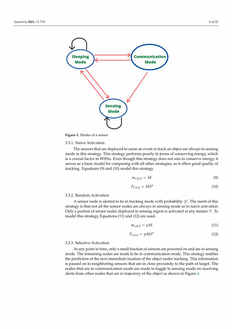
The general strategies in TT are naive activation, random activation, selective activa-tion, and periodic activation. The sensor nodes that are deployed in a sensing region fortracking targets work in three modes viz., communication mode, sensing mode, and dataprocessing mode. Figure 3 displays the various operating modes of a sensor.

Symmetry 2021, 13, 719 6 of 22

Symmetry 2021, 13, x FOR PEER REVIEW 6 of 23

3.3. Strategies in Target Tracking The general strategies in TT are naive activation, random activation, selective acti-

vation, and periodic activation. The sensor nodes that are deployed in a sensing region for tracking targets work in three modes viz., communication mode, sensing mode, and data processing mode. Figure 3 displays the various operating modes of a sensor.

Figure 3. Modes of a sensor.

3.3.1. Naive Activation The sensors that are deployed to sense an event or track an object are always in

sensing mode in this strategy. This strategy performs poorly in terms of conserving en-ergy, which is a crucial factor in WSNs. Even though this strategy does not aim to con-serve energy, it serves as a basic model for comparing with all other strategies, as it offers good quality of tracking. Equations (9) and (10) model this strategy. 𝑚 , = 𝑀 (9) 𝑃 . = 𝑀𝑆 (10)

3.3.2. Random Activation A sensor node is alerted to be in tracking mode with probability ‘p’. The merit of this

strategy is that not all the sensor nodes are always in sensing mode as in naive activation. Only a portion of sensor nodes deployed in sensing region is activated at any instant ‘t’. To model this strategy, Equations (11) and (12) are used. 𝑚 , = 𝑝𝑀 (11)𝑃 , = 𝑝𝑀𝑆 (12)

3.3.3. Selective Activation At any point in time, only a small fraction of sensors are powered on and are in

sensing mode. The remaining nodes are made to be in communication mode. This strat-egy enables the prediction of the next immediate location of the object under tracking.

Figure 3. Modes of a sensor.

3.3.1. Naive Activation

The sensors that are deployed to sense an event or track an object are always in sensingmode in this strategy. This strategy performs poorly in terms of conserving energy, whichis a crucial factor in WSNs. Even though this strategy does not aim to conserve energy, itserves as a basic model for comparing with all other strategies, as it offers good quality oftracking. Equations (9) and (10) model this strategy.

ms,NA = M (9)

Pt.NA = MSα (10)

3.3.2. Random Activation

A sensor node is alerted to be in tracking mode with probability ‘p’. The merit of thisstrategy is that not all the sensor nodes are always in sensing mode as in naive activation.Only a portion of sensor nodes deployed in sensing region is activated at any instant ‘t’. Tomodel this strategy, Equations (11) and (12) are used.

ms,RA = pM (11)

Pt,NA = pMSα (12)

3.3.3. Selective Activation

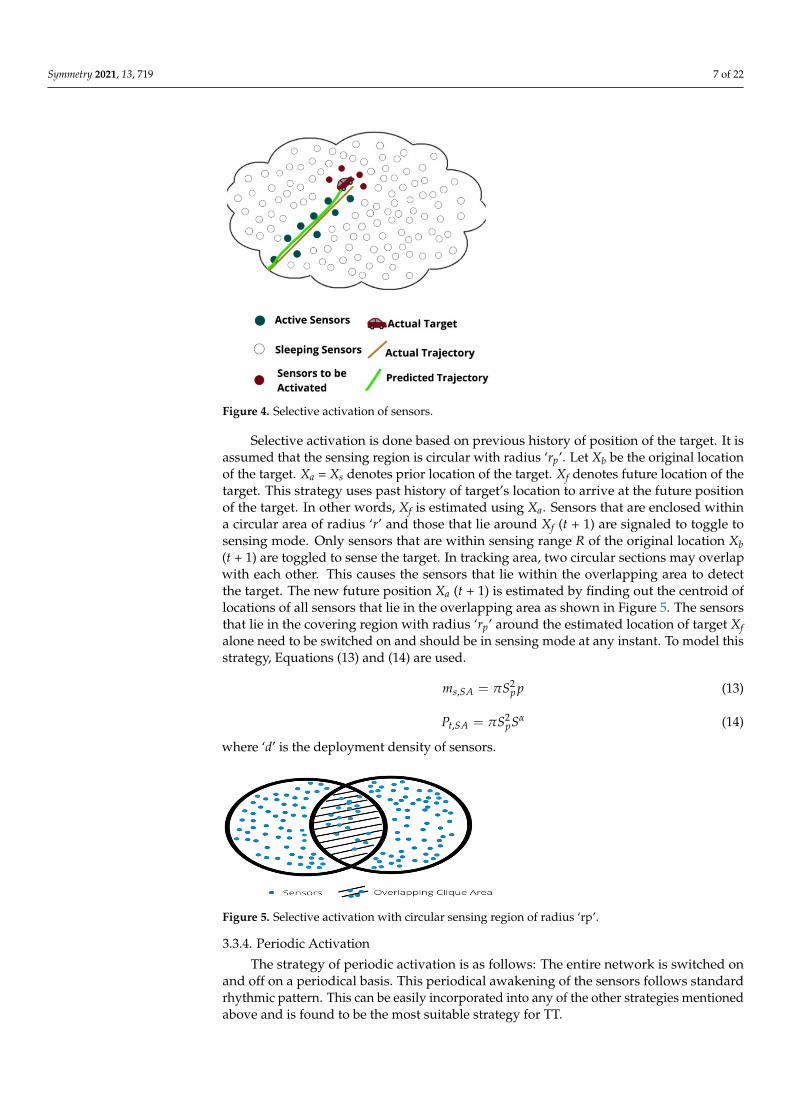
At any point in time, only a small fraction of sensors are powered on and are in sensingmode. The remaining nodes are made to be in communication mode. This strategy enablesthe prediction of the next immediate location of the object under tracking. This informationis passed on to neighboring sensors that are in close proximity to the path of target. Thenodes that are in communication mode are made to toggle to sensing mode on receivingalerts from other nodes that are in trajectory of the object as shown in Figure 4.

Symmetry 2021, 13, 719 7 of 22

Symmetry 2021, 13, x FOR PEER REVIEW 7 of 23

This information is passed on to neighboring sensors that are in close proximity to the path of target. The nodes that are in communication mode are made to toggle to sensing mode on receiving alerts from other nodes that are in trajectory of the object as shown in Figure 4.

Figure 4. Selective activation of sensors.

Selective activation is done based on previous history of position of the target. It is assumed that the sensing region is circular with radius ‘rp’. Let Xb be the original location of the target. Xa = Xs denotes prior location of the target. Xf denotes future location of the target. This strategy uses past history of target’s location to arrive at the future position of the target. In other words, Xf is estimated using Xa. Sensors that are enclosed within a circular area of radius ‘r’ and those that lie around Xf (t + 1) are signaled to toggle to sensing mode. Only sensors that are within sensing range R of the original location Xb (t + 1) are toggled to sense the target. In tracking area, two circular sections may overlap with each other. This causes the sensors that lie within the overlapping area to detect the tar-get. The new future position Xa (t + 1) is estimated by finding out the centroid of locations of all sensors that lie in the overlapping area as shown in Figure 5. The sensors that lie in the covering region with radius ‘rp’ around the estimated location of target Xf alone need to be switched on and should be in sensing mode at any instant. To model this strategy, Equations (13) and (14) are used. 𝑚 , = 𝜋𝑆 𝑝 (13)𝑃 , = 𝜋𝑆 𝑆 (14)

where ‘d’ is the deployment density of sensors.

3.3.4. Periodic Activation The strategy of periodic activation is as follows: The entire network is switched on

and off on a periodical basis. This periodical awakening of the sensors follows standard rhythmic pattern. This can be easily incorporated into any of the other strategies men-tioned above and is found to be the most suitable strategy for TT.

Figure 4. Selective activation of sensors.

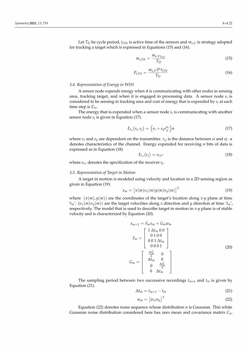
Selective activation is done based on previous history of position of the target. It isassumed that the sensing region is circular with radius ‘rp’. Let Xb be the original locationof the target. Xa = Xs denotes prior location of the target. Xf denotes future location of thetarget. This strategy uses past history of target’s location to arrive at the future positionof the target. In other words, Xf is estimated using Xa. Sensors that are enclosed withina circular area of radius ‘r’ and those that lie around Xf (t + 1) are signaled to toggle tosensing mode. Only sensors that are within sensing range R of the original location Xb(t + 1) are toggled to sense the target. In tracking area, two circular sections may overlapwith each other. This causes the sensors that lie within the overlapping area to detectthe target. The new future position Xa (t + 1) is estimated by finding out the centroid oflocations of all sensors that lie in the overlapping area as shown in Figure 5. The sensorsthat lie in the covering region with radius ‘rp’ around the estimated location of target Xfalone need to be switched on and should be in sensing mode at any instant. To model thisstrategy, Equations (13) and (14) are used.

ms,SA = πS2p p (13)

Pt,SA = πS2pSα (14)

where ‘d’ is the deployment density of sensors.

Symmetry 2021, 13, x FOR PEER REVIEW 8 of 23

Figure 5. Selective activation with circular sensing region of radius ‘rp’.

Let 𝑇 be cycle period,𝑡 is active time of the sensors and 𝑚 , is strategy adopted for tracking a target which is expressed in Equations (15) and (16). 𝑚 , = 𝑚 ,𝑇 (15)

𝑃 , = 𝑚 , 𝑆 𝑡𝑇 (16)

3.4. Representation of Energy in WSN A sensor node expends energy when it is communicating with other nodes in sens-

ing area, tracking target, and when it is engaged in processing data. A sensor node si is considered to be sensing in tracking area and cost of energy that is expended by si at each time step is Erx.

The energy that is expended when a sensor node si is communicating with another sensor node sj is given in Equation (17). 𝐸 𝑠 , 𝑠 = 𝑒 + 𝑒 𝑟 𝑛 (17)

where 𝑒 and 𝑒 are dependent on the transmitter. 𝑟 is the distance between si and sj. α denotes characteristics of the channel. Energy expended for receiving n bits of data is expressed as in Equation (18). 𝐸 𝑠 = 𝑒 (18)

where 𝑒 denotes the specification of the receiver sj.

3.5. Representation of Target in Motion A target in motion is modeled using velocity and location in a 2D sensing region as

given in Equation (19). 𝑥 = 𝑥(𝑚)𝑣 (𝑚)𝑦(𝑚)𝑣 (𝑚) (19)

where (𝑥(𝑚), 𝑦(𝑚)) are the coordinates of the target’s location along x-y plane at time ‘tm‘. (𝑣 (𝑚)𝑣 (𝑚)) are the target velocities along x direction and y direction at time ‘tm‘, respectively. The model that is used to describe target in motion in x-y plane is of stable velocity and is characterized by Equation (20).

Figure 5. Selective activation with circular sensing region of radius ‘rp’.

3.3.4. Periodic Activation

The strategy of periodic activation is as follows: The entire network is switched onand off on a periodical basis. This periodical awakening of the sensors follows standardrhythmic pattern. This can be easily incorporated into any of the other strategies mentionedabove and is found to be the most suitable strategy for TT.

Symmetry 2021, 13, 719 8 of 22

Let TD be cycle period, tON is active time of the sensors and ms,V is strategy adoptedfor tracking a target which is expressed in Equations (15) and (16).

ms,PA =ms,VtON

TD(15)

Pt,PA =ms,VSαtON

TD(16)

3.4. Representation of Energy in WSN

A sensor node expends energy when it is communicating with other nodes in sensingarea, tracking target, and when it is engaged in processing data. A sensor node si isconsidered to be sensing in tracking area and cost of energy that is expended by si at eachtime step is Erx.

The energy that is expended when a sensor node si is communicating with anothersensor node sj is given in Equation (17).

Etx

(si, sj

)=(

et + edrαcij

)n (17)

where et and ed are dependent on the transmitter. rij is the distance between si and sj. αdenotes characteristics of the channel. Energy expended for receiving n bits of data isexpressed as in Equation (18).

Erx

(sj)= erxn (18)

where erx denotes the specification of the receiver sj.

3.5. Representation of Target in Motion

A target in motion is modeled using velocity and location in a 2D sensing region asgiven in Equation (19).

xm =[x(m)vx(m)y(m)vy(m)

]T (19)

where (x(m), y(m)) are the coordinates of the target’s location along x-y plane at time‘tm’. (vx(m)vy(m)) are the target velocities along x direction and y direction at time ‘tm’,respectively. The model that is used to describe target in motion in x-y plane is of stablevelocity and is characterized by Equation (20).

xm+1 = Fmxm + Gmwm

Fm =

1 ∆tm 0 0

0 1 0 00 0 1 ∆tm

0 0 0 1

Gm =

∆t2

m2 0

∆tm 0

0 ∆t2m

20 ∆tm

(20)

The sampling period between two successive recordings tm+1 and tm is given byEquation (21).

∆tm = tm+1 − tm (21)

wm =[wxwy

]T (22)

Equation (22) denotes noise sequence whose distribution n is Gaussian. This whiteGaussian noise distribution considered here has zero mean and covariance matrix Cw.

Symmetry 2021, 13, 719 9 of 22

Therefore, noise across x and y axis is modeled using wx and wy. Covariance matrix Cw isgiven by Equation (23).

Cw =

[σ2

wx 00 σ2

wy

](23)

A few assumptions made in the model are summarized below:

• wx is not correlated to wy.• Covariance and mean of multiplicative noise is given.• Covariance and mean of additive noise is also given.• Another crucial assumption is that if noises are absent, then it is fairly straightforward

to determine position of the target.

4. Materials and Methods4.1. Proposed TDTT Model

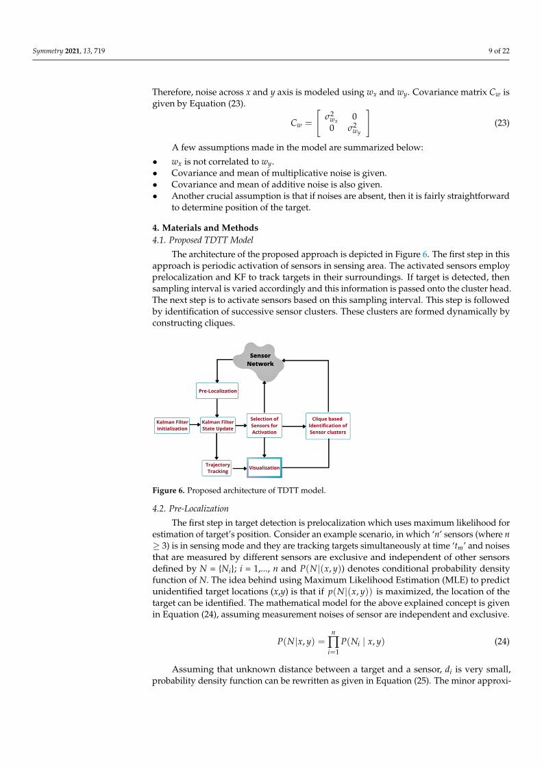
The architecture of the proposed approach is depicted in Figure 6. The first step in thisapproach is periodic activation of sensors in sensing area. The activated sensors employprelocalization and KF to track targets in their surroundings. If target is detected, thensampling interval is varied accordingly and this information is passed onto the cluster head.The next step is to activate sensors based on this sampling interval. This step is followedby identification of successive sensor clusters. These clusters are formed dynamically byconstructing cliques.

Symmetry 2021, 13, x FOR PEER REVIEW 11 of 23

𝑃((x,y)|N) = ( | , ) ( , )( ) (31)

The prior probability density function of (x,y) that is known to sensor nodes is pb(x,y). However, pb (x,y) does not include any information on the previous position of the target under consideration. pb (x,y) is uniform, always in sensing region. Considering this, 𝑃(𝑥, 𝑦|𝑁) is shown in Equation (32). 𝑃(𝑥, 𝑦|𝑁) = α 𝑃((𝑁|𝑥, 𝑦) (32)

(x,y) is independent of α. Therefore, 𝑃 (𝑥, 𝑦|𝑁) = ( ( , ))( ) ∏ (33)

Figure 6. Proposed architecture of TDTT model.

The equation after prelocalization and approximation is given in Equation (34). 𝑓(𝑥, 𝑦) ≅ 𝑓(��, 𝑦) + 12 𝑥 − ��𝑦 − 𝑦 𝐻(��, 𝑦) 𝑥 − ��𝑦 − 𝑦 (34)𝐻(��, 𝑦) denote Hessian matrix shown by Equation (35).

𝐻(��, 𝑦) = ⎣⎢⎢⎢⎡𝜕 𝑓(𝑥, 𝑦)𝜕𝑥 𝜕 𝑓(𝑥, 𝑦)𝜕𝑥𝜕𝑦𝜕 𝑓(𝑥, 𝑦)𝜕𝑦𝜕𝑥 𝜕 𝑓(𝑥, 𝑦)𝜕𝑦 ⎦⎥⎥⎥

⎤ 𝑥 = �� , 𝑦 = 𝑦 (35)

𝑃 (𝑥, 𝑦|𝑁) ≅ 𝛽 𝑒𝑥𝑝 − 𝑥 − ��𝑦 − 𝑦 𝐻(��, 𝑦) 𝑥 − ��𝑦 − 𝑦 where 𝛽 is a constant (36)

4.4. Choosing Sampling Period Assuming sampling period ∆𝑡 to be uniform does not make the representation

energy efficient and cannot adapt to the trajectory of target. The interval of sampling is denoted by 𝑇 , 𝑇 . This interval is chosen so that 𝑇 is greater than the time taken for communication, sensing, and processing, whereas, 𝑇 should not be arbitrarily larger values, as the model has to deal with changing trajectory of the object. Considering the difficulty of choosing sampling period and predictions made in covariance matrix, for approximation, a time update is performed to calculate the sampling period.

Uncertainty in estimated position is shown in Equation (37).

Figure 6. Proposed architecture of TDTT model.

4.2. Pre-Localization

The first step in target detection is prelocalization which uses maximum likelihood forestimation of target’s position. Consider an example scenario, in which ‘n’ sensors (where n≥ 3) is in sensing mode and they are tracking targets simultaneously at time ‘tm’ and noisesthat are measured by different sensors are exclusive and independent of other sensorsdefined by N = {Ni}; i = 1,..., n and P(N|(x, y)) denotes conditional probability densityfunction of N. The idea behind using Maximum Likelihood Estimation (MLE) to predictunidentified target locations (x,y) is that if p(N|(x, y)) is maximized, the location of thetarget can be identified. The mathematical model for the above explained concept is givenin Equation (24), assuming measurement noises of sensor are independent and exclusive.

P(N|x, y) =n

∏i=1

P(Ni | x, y) (24)

Assuming that unknown distance between a target and a sensor, di is very small,probability density function can be rewritten as given in Equation (25). The minor approxi-

Symmetry 2021, 13, 719 10 of 22

mation done is negligible in probability density function and it is a well-known fact thatKF is very resistant towards small variations in measurement noise.

P({Ni|x, y}) ∼=1√

2πσNi

exp

{−[[1 + µr]di − Ni

]22 σ2

Ni

}(25)

where Ni = Ni − µn and denotes actual calculated measurement. Based on Equation (26),MLE of (x,y) is calculated using Equation (26).

(x, y) = argmin(x, y) f (x, y) (26)

f (x, y) =n

∑i=1

[[1 + µr]di − Ni

]22 σ2

Ni

(27)

Equation (27) has to be minimized and this is quite difficult as f (x,y) is not linear.Newton-Raphson method, an iterative optimized solution, is used to process this non-linear function. This step works as follows:

Step 1: compute x(i+1) and y(i+1) using Equation (28) where h is step size.[x(i+1)

y(i+1)

]=

[xi

yi

]− hH−1

(x(i), y(i)

).∇ f T

(x(i), y(i)

)∇ f(

x(i), y(i))=[

∂ f (x,y)∂x

∂ f (x,y)∂y

]x=x(i), y=y(i)

H(

x(i), y(i))=

∂2 f (x,y)∂x2

∂2 f (x,y)∂x∂y

∂2 f (x,y)∂y∂x

∂2 f (x,y)∂y2

x=x(i),y=y(i)

(28)

Step 2: iterate step 1 until∣∣∣x(i+1) − x(i)

∣∣∣ < ε and∣∣∣y(i+1) − y(i)

∣∣∣ < ε with step size ‘1′

and ε > 0 is a fixed limit.The first and third terms of the estimated value xm|m−1 of KF are x1

m|m−1 and x3m|m−1.

This iterative method converges and gives a global minimum in successive iterations. Theinitial values assigned to first and third terms of initial prediction in KF play an importantrole in making this prediction an accurate one, based on the constraint that the samplingperiod is limited.

4.3. Position Estimation Using KF

After prelocalization, the result is the changed measurement.

Nm = [x(m) y(m)]T (29)

Equation (29) has linear representation which is shown in Equation (30).

Nm =

[1 0 0 00 0 1 0

]xm + vm = Zxm + Vm (30)

Vm denotes measurement noise that is converted after prelocalization. This Nm valueis to be used in KF. Equation (31) shows Baye’s rule for posterior probability distribution.

P((x, y)|N) =P(N|x, y) Pb(x, y)

P(N)(31)

The prior probability density function of (x,y) that is known to sensor nodes is pb(x,y).However, pb (x,y) does not include any information on the previous position of the target

Symmetry 2021, 13, 719 11 of 22

under consideration. pb (x,y) is uniform, always in sensing region. Considering this,P(x, y|N) is shown in Equation (32).

P(x, y|N) = α P((N|x, y) (32)

(x, y) is independent of α. Therefore, P (x, y|N) =α Xexp(− f (x, y))

(2π)n2 ∏n

i=1 σNi

(33)

The equation after prelocalization and approximation is given in Equation (34).

f (x, y) ∼= f (x, y) +12

[x− xy− y

]T

H(x, y)[

x− xy− y

](34)

H(x, y) denote Hessian matrix shown by Equation (35).

H(x, y) =

∂2 f (x,y)∂x2

∂2 f (x,y)∂x∂y

∂2 f (x,y)∂y∂x

∂2 f (x,y)∂y2

x = x , y = y (35)

P (x, y|N) ∼= β exp

(−1

2

[x− xy− y

]T

H(x, y)[

x− xy− y

])where β is a constant (36)

4.4. Choosing Sampling Period

Assuming sampling period ∆tm to be uniform does not make the representationenergy efficient and cannot adapt to the trajectory of target. The interval of sampling isdenoted by [Tmin, Tmax]. This interval is chosen so that Tmin is greater than the time takenfor communication, sensing, and processing, whereas, Tmax should not be arbitrarily largervalues, as the model has to deal with changing trajectory of the object. Considering thedifficulty of choosing sampling period and predictions made in covariance matrix, forapproximation, a time update is performed to calculate the sampling period.

Uncertainty in estimated position is shown in Equation (37).

∅ (m + 1 | m) = trace(∑(∆tm)

)= (σ11 + σ33) + (2σ12 + 2σ34)∆tm + (σ22 + σ44)∆tm

2 +23

q∆tm3

= ∅ (m | m) + (σ11 + σ33) + (2σ12 + 2σ34)∆tm + (σ22 + σ44)∆tm2 +

23

q∆tm3

(37)

If P (m | m) > 0 and c(m) > 0 and ∅0 > ∅ (m |m) > 0, then there is the possibility of areal root that is positive. Based on Equation (37), two possible modes of operation in TT arequick tracking and tracking management. When ∅ (m | m) > 0 is not satisfied, then quicktracking is employed, usually when tracking is initiated or when target changes the course.The sampling period is selected as Tmin. When there is an acceptable accuracy in recentand estimated tracking, tracking management mode is employed. The sampling periodis greater than Tmin and the value is the least value among positive root of Equation (37)and Tmax.

4.5. Choosing Sensors to Be in Sensing Mode

After determining sampling period values, sensors will be chosen for sensing. Arelated assumption is that sensor nodes store the characteristics of all of its neighboringsensor nodes, namely, position and sensing range. The cluster head chosen now evaluatesprobability density function of other sensors, considering the estimated position of targetand associated covariance matrix. The neighboring sensor nodes are denoted as a set S.

Symmetry 2021, 13, 719 12 of 22

Probability density function is computed and sensor with high probability density functionat the next step is chosen as the first and foremost member of cluster at time m+1.

g(m+1)1 = argSi max{Pr(Si) : Si ∈ S} (38)

where (m + 1) is the (m + 1)th time step.The second sensor of the cluster is chosen based on

g(m+1)2 = argSi max

{Pr

(g(m+1)

1 , Si

): Si ∈ S\

{g(k+1)

1

}}(39)

Pr

(g(m+1)

1 , Si

)is joint distribution probability of g(m+1)

1 and Si.

S\{

g(k+1)1

}is the set of all sensors S exclusive of g(m+1)

1 .This is employed to choose all other sensors. The jth sensor is chosen as,

g(m+1)j = argSi max

{Pr

(g(m+1)

1 , g(m+1)2 , . . . ., g(m+1)

i−1 , Si

): Si ∈ S\

y=i−1∪

y=1

{g(k+1)

y

}}(40)

The selection of sensors is ended when joint distribution probability is greater than aspecified limit ∅t. The tasking cluster for the next iteration is given in Equation (41).

G(m + 1) ={

g(k+1)j : j = 1, 2, . . . , n

}(41)

4.6. Identification of Successive Cliques

A target ‘t1’ is assumed to have unpredictable velocity such that ‘t1’ is assumed tomove in a complex way and it is difficult to represent the complexity. The sequence ofsteps that is required to identify the clique in which the target ‘t1’ is travelling is:

• t1 is detected by s3.• s3 exchanges this information with the neighbors.• s3 receives the information from all other neighbors and conducts the comparison

between its own information and the neighbors’ information.• All the neighboring sensor nodes are in sensing mode and t1 is tracked within the

sensing region and the immediate neighbor closest to t1 maintains the required infor-mation.

• The clique in which t1 moves is constructed.

t1’s movement from F1 to any other clique Fj is tracked using monitor and backupoperation. This operation is based on all locations of t1, considering the current motiontrajectory. The next step to be carried out is calculating the direction of target’s motion. Theclique that is constructed in the previous step is represented by set Mn,

Mn ={

lj, θm, θ′m, vmaxn , vmax′

n

}; (42)

To calculate the next position of target, it is necessary to calculate S′ = Sj; j = 1, 2, . . . ;.The median of this set S′ is calculated and stored in Smedian. lj+1 is calculated and lj is

updated by lj+1 and stored. The moving path is calculated based on lj; j = 1, 2, . . . ;. t1’scenter of gravity position is used to find t1’s position. t1 may follow any dynamic pathsuch as travelling in a linear fashion, turning towards right or left, and performing U turn.

In this scenario, time instance of S is subdivided into discrete series, namely S1, S2...In each Si, the duration is set to 1. The direction of movement and target is denoted by θ.The state of motion of target t1 at time S is denoted by

Dt1 ={

lj, θh, θ′h, vmaxt1

, vmax′t1

}(43)

θh and θ′h are the angle of tracking and the angle of maneuvering.

Symmetry 2021, 13, 719 13 of 22

vmaxt1

and vmax′t1

are the velocity of straight movement and the velocity of maneuver-ing, respectively.

The distance covered by target t1 can be calculated by each node in the following ways:Case 1: Straight Line

θh = 0; t is in straight line motion

Dh = vmaxt

(44)

Case 2: Curved Lineθh ∈ (−π, π)&h1 < 1, this denotes t1 is moving in random way (curved). In order

to calculate the sequence of locations, it is necessary to introduce δ and r, δ denotes thecurve made by the manoeuvring of the target and r denotes the distance covered by t1 inθh direction.

The length of the path due to straight line movement of t1 is p, then

δ = θ′hP (45)

h1 =δ

Vtmax′(46)

θ′h =Vtmax

ptan(θh) (47)

Dh = 2p sin(

θ′h2

)+ Vtmax

(1−

θ′h pVtmax′

)(48)

Case 3:θh ∈ (−π, π)&h1 ≥ 1 (49)

Dh = 2p sin(

Vtmax′

2p

)(50)

Knowing the current location of t1 and h, the estimated location of lj+1 with approxi-mate coordinates

(xj+1, yj+1

)of t1 at j + 1 is

xj+1 = xj + Dt1 cos θh (51)

yj+1 = yj − Dt1 sin θh (52)

All positions of t1 can be calculated by changing θh between −π and π.Knowing clique Fj, where t1 is in motion currently, the sequence of positions is

obtained by the previous step. An alert message is issued to the neighbors of Fi. If the nodethat receives the alert is the requested node, then all those nodes are grouped in Fj+1 andother cliques. If it does not receive the signal, then the node is in awakening state. If t1is detected and signal is received, then exchange communication with new backup andproceed with calculating the new maneuver of t1. Finally, if target t1 is detected in Fj+1 thenlj is the new location. Fj = Fj+1 is the new clique.

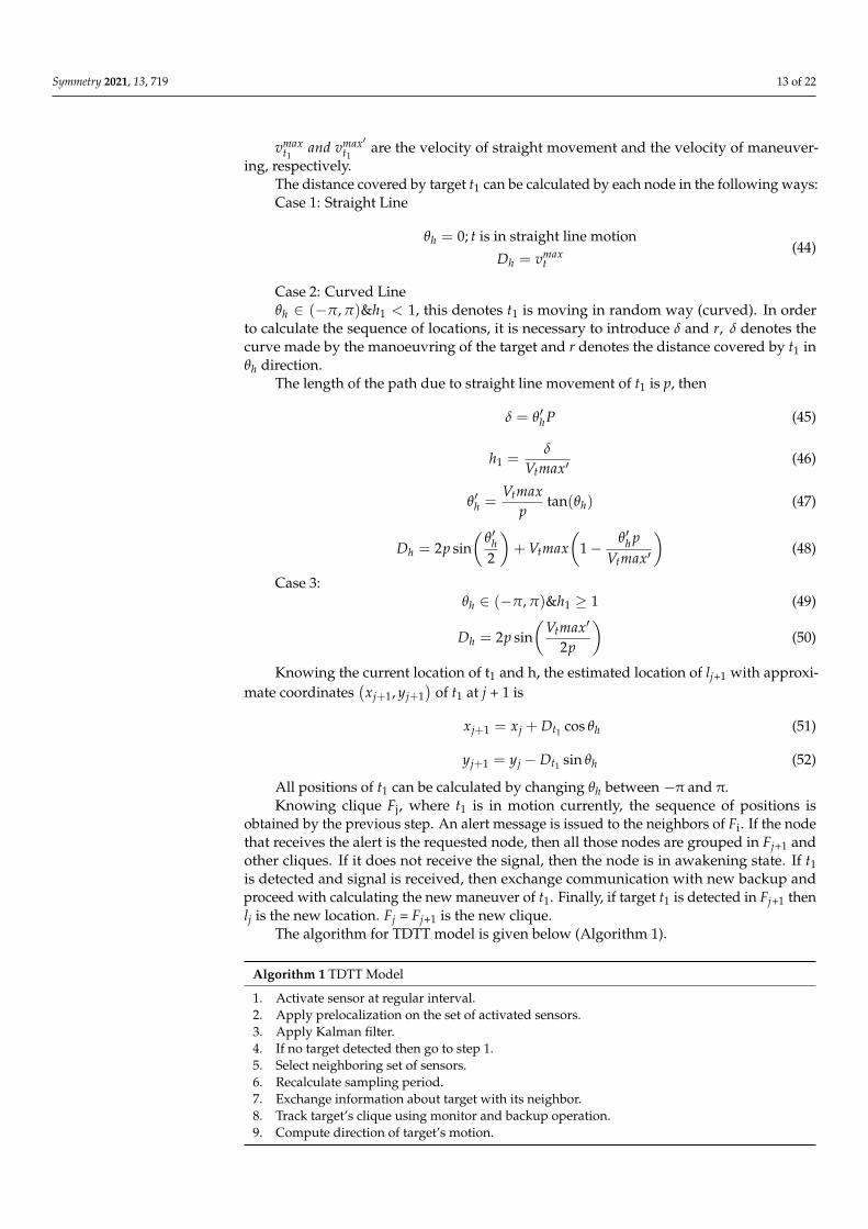
The algorithm for TDTT model is given below (Algorithm 1).

Algorithm 1 TDTT Model

1. Activate sensor at regular interval.2. Apply prelocalization on the set of activated sensors.3. Apply Kalman filter.4. If no target detected then go to step 1.5. Select neighboring set of sensors.6. Recalculate sampling period.7. Exchange information about target with its neighbor.8. Track target’s clique using monitor and backup operation.9. Compute direction of target’s motion.

Symmetry 2021, 13, 719 14 of 22

5. Results

In this section, the performance of the proposed approach is evaluated in two differentsimulation scenarios. The first and second scenario were simulated both in ideal andnon-ideal setup to test the performance of tracking the target using KF and clique-basedapproach. The third scenario was simulated and performance of our approach is comparedwith DOT and FaceTrack approaches. Both DOT and FaceTrack authors specify an approachthat constructs faces to track a target. TDTT constructs cliques similar to Face construction.Therefore, these two approaches are used for comparison. The simulation was performedon a 1000 × 1000 m2 field with around 950 sensors in a 40 × 40 grid and a sensing range of100 m per sensor. The monitored area of this simulation was set to 1000 m and parameterswere captured by playing the simulation until 2500 s.

5.1. Scenario 1

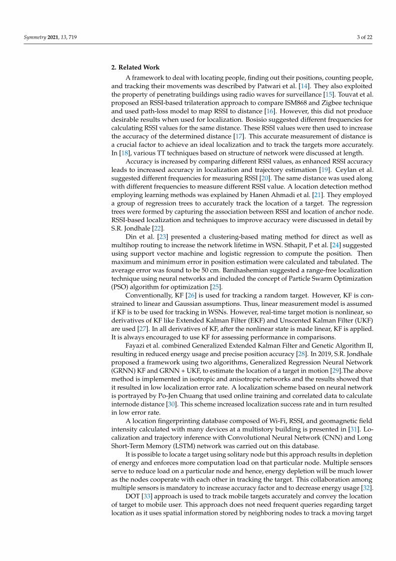
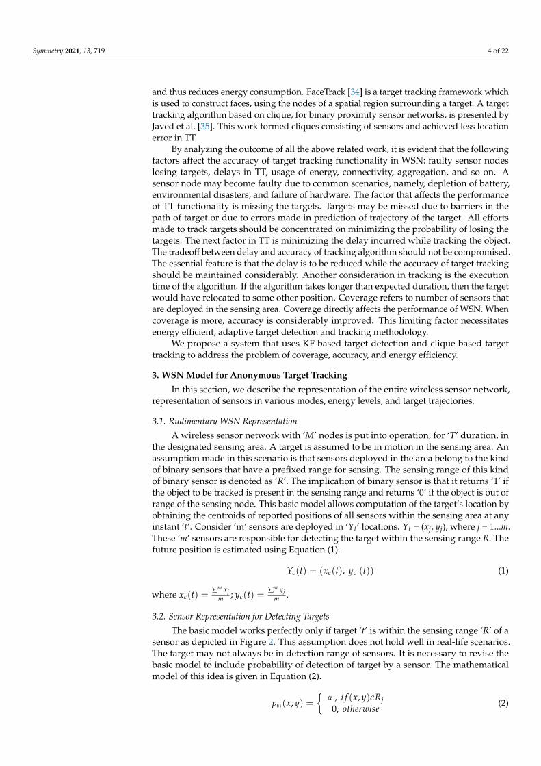
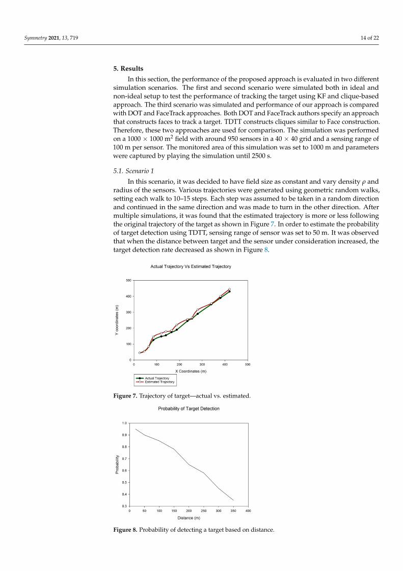
In this scenario, it was decided to have field size as constant and vary density ρ andradius of the sensors. Various trajectories were generated using geometric random walks,setting each walk to 10–15 steps. Each step was assumed to be taken in a random directionand continued in the same direction and was made to turn in the other direction. Aftermultiple simulations, it was found that the estimated trajectory is more or less followingthe original trajectory of the target as shown in Figure 7. In order to estimate the probabilityof target detection using TDTT, sensing range of sensor was set to 50 m. It was observedthat when the distance between target and the sensor under consideration increased, thetarget detection rate decreased as shown in Figure 8.

Symmetry 2021, 13, x FOR PEER REVIEW 15 of 23

Figure 7. Trajectory of target—actual vs. estimated.

Figure 8. Probability of detecting a target based on distance.

This observation led to another experiment in which we varied the density of sen-sors and the error in localizing the target and tracking the target was calculated. Fixing the size of the field and the radius as constant, the number of sensors in the field was varied from 100 to 650. Then the simulation was performed for uniform regular and random arrangement of sensors. As per spatial resolution theorem, an increase in density of sensors results in a decrease in error estimation. It was noticed that as the number of sensors increased, error in difference between the original and estimated trajectory de-creased as shown in Figure 9. There is a slight deviation between theoretical value and estimated error averaged over 55 rounds of random walk paths. The distribution of sensors was kept constant at 950 sensors but their sensing radius was changed from 50 m to 350 m. Error in estimation was found to be decreasing with increase in radius R as shown in Figure 10. The calculated error was more or less in line with the theoretical value.

Figure 7. Trajectory of target—actual vs. estimated.

Symmetry 2021, 13, x FOR PEER REVIEW 15 of 23

Figure 7. Trajectory of target—actual vs. estimated.

Figure 8. Probability of detecting a target based on distance.

This observation led to another experiment in which we varied the density of sen-sors and the error in localizing the target and tracking the target was calculated. Fixing the size of the field and the radius as constant, the number of sensors in the field was varied from 100 to 650. Then the simulation was performed for uniform regular and random arrangement of sensors. As per spatial resolution theorem, an increase in density of sensors results in a decrease in error estimation. It was noticed that as the number of sensors increased, error in difference between the original and estimated trajectory de-creased as shown in Figure 9. There is a slight deviation between theoretical value and estimated error averaged over 55 rounds of random walk paths. The distribution of sensors was kept constant at 950 sensors but their sensing radius was changed from 50 m to 350 m. Error in estimation was found to be decreasing with increase in radius R as shown in Figure 10. The calculated error was more or less in line with the theoretical value.

Figure 8. Probability of detecting a target based on distance.

Symmetry 2021, 13, 719 15 of 22

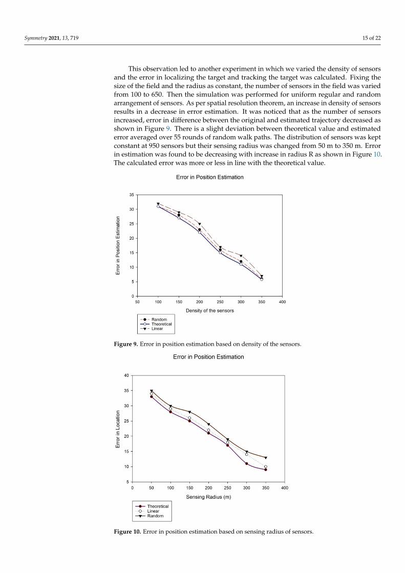
This observation led to another experiment in which we varied the density of sensorsand the error in localizing the target and tracking the target was calculated. Fixing thesize of the field and the radius as constant, the number of sensors in the field was variedfrom 100 to 650. Then the simulation was performed for uniform regular and randomarrangement of sensors. As per spatial resolution theorem, an increase in density of sensorsresults in a decrease in error estimation. It was noticed that as the number of sensorsincreased, error in difference between the original and estimated trajectory decreased asshown in Figure 9. There is a slight deviation between theoretical value and estimatederror averaged over 55 rounds of random walk paths. The distribution of sensors was keptconstant at 950 sensors but their sensing radius was changed from 50 m to 350 m. Errorin estimation was found to be decreasing with increase in radius R as shown in Figure 10.The calculated error was more or less in line with the theoretical value.

Symmetry 2021, 13, x FOR PEER REVIEW 16 of 23

Figure 9. Error in position estimation based on density of the sensors.

Figure 10. Error in position estimation based on sensing radius of sensors.

5.2. Scenario 2 This scenario was simulated by making the following assumptions: sensing range of

all the sensors was fixed. The number of sensors was varied from 100 to 650. For each variation of sensor density, the target was deployed either closer to or far off from the sensor arrangement. Initially, the target was deployed closer to the sensor arrangements for all variations in number of sensors and the result was displayed in Figure 9. Then it was decided to vary the position of target deployment for different sensor densities to

Figure 9. Error in position estimation based on density of the sensors.

Symmetry 2021, 13, x FOR PEER REVIEW 16 of 23

Figure 9. Error in position estimation based on density of the sensors.

Figure 10. Error in position estimation based on sensing radius of sensors.

5.2. Scenario 2 This scenario was simulated by making the following assumptions: sensing range of

all the sensors was fixed. The number of sensors was varied from 100 to 650. For each variation of sensor density, the target was deployed either closer to or far off from the sensor arrangement. Initially, the target was deployed closer to the sensor arrangements for all variations in number of sensors and the result was displayed in Figure 9. Then it was decided to vary the position of target deployment for different sensor densities to

Figure 10. Error in position estimation based on sensing radius of sensors.

Symmetry 2021, 13, 719 16 of 22

5.2. Scenario 2

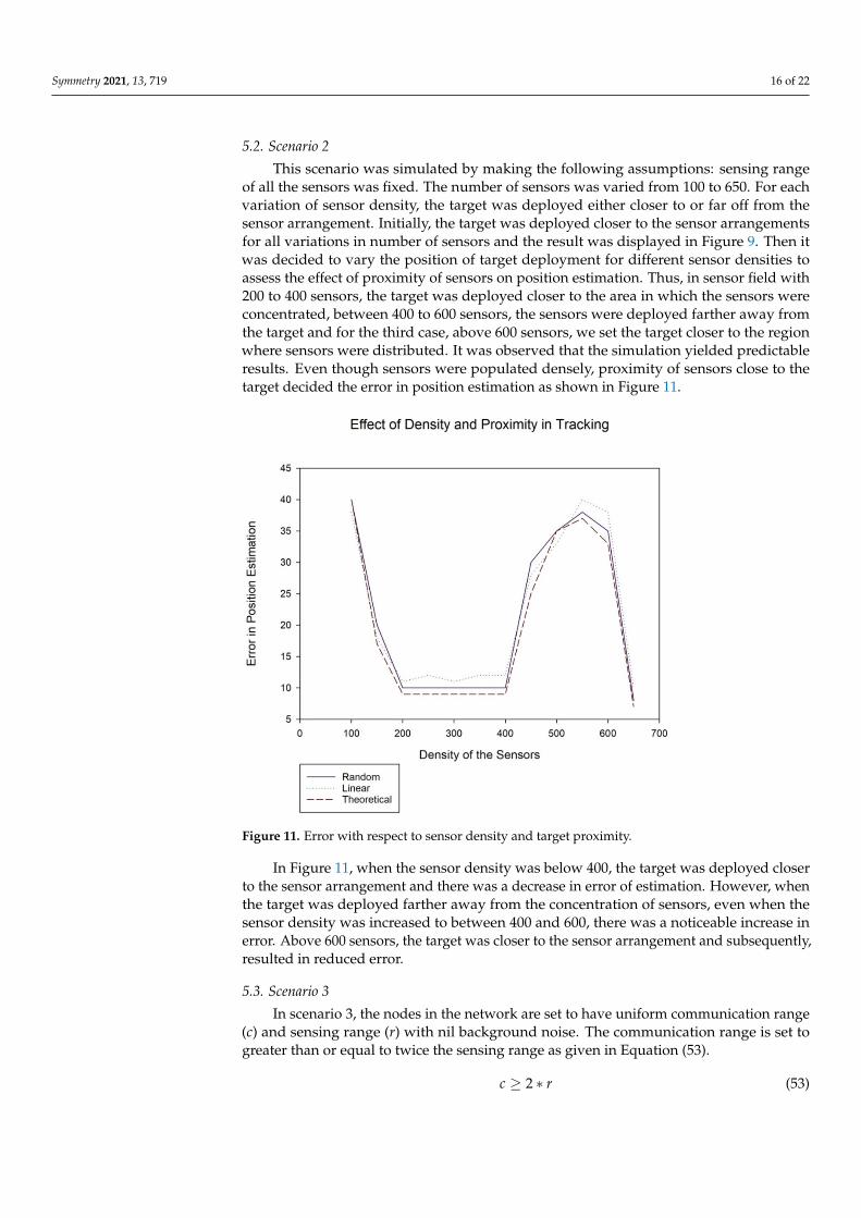
This scenario was simulated by making the following assumptions: sensing rangeof all the sensors was fixed. The number of sensors was varied from 100 to 650. For eachvariation of sensor density, the target was deployed either closer to or far off from thesensor arrangement. Initially, the target was deployed closer to the sensor arrangementsfor all variations in number of sensors and the result was displayed in Figure 9. Then itwas decided to vary the position of target deployment for different sensor densities toassess the effect of proximity of sensors on position estimation. Thus, in sensor field with200 to 400 sensors, the target was deployed closer to the area in which the sensors wereconcentrated, between 400 to 600 sensors, the sensors were deployed farther away fromthe target and for the third case, above 600 sensors, we set the target closer to the regionwhere sensors were distributed. It was observed that the simulation yielded predictableresults. Even though sensors were populated densely, proximity of sensors close to thetarget decided the error in position estimation as shown in Figure 11.

Symmetry 2021, 13, x FOR PEER REVIEW 17 of 23

assess the effect of proximity of sensors on position estimation. Thus, in sensor field with 200 to 400 sensors, the target was deployed closer to the area in which the sensors were concentrated, between 400 to 600 sensors, the sensors were deployed farther away from the target and for the third case, above 600 sensors, we set the target closer to the region where sensors were distributed. It was observed that the simulation yielded predictable results. Even though sensors were populated densely, proximity of sensors close to the target decided the error in position estimation as shown in Figure 11.

In Figure 11, when the sensor density was below 400, the target was deployed closer to the sensor arrangement and there was a decrease in error of estimation. However, when the target was deployed farther away from the concentration of sensors, even when the sensor density was increased to between 400 and 600, there was a noticeable increase in error. Above 600 sensors, the target was closer to the sensor arrangement and subse-quently, resulted in reduced error.

Figure 11. Error with respect to sensor density and target proximity.

5.3. Scenario 3 In scenario 3, the nodes in the network are set to have uniform communication range

(c) and sensing range (r) with nil background noise. The communication range is set to greater than or equal to twice the sensing range as given in Equation (53). 𝑐 ≥ 2 ∗ 𝑟 (53)

The sensing range of nodes is set to 100 m and communication range of nodes is 200 m. Node–sink synchronization happens in the first 1–10 ms of the simulation. The tar-get’s speed is 1 m/s.

Initially, all sensor nodes collect information regarding neighbor nodes. The target is deployed in the simulated network at an arbitrary time and in a random spot. The target moves in random fashion in the sensing area. Target detection is triggered when the target is detected by the sensor nodes in the network and KF is employed to assess the location of the deployed target. Then the clique is constructed as the target moves along a trajectory. Now the sensors are enabled to track the target. Over 150 simulation runs are

Figure 11. Error with respect to sensor density and target proximity.

In Figure 11, when the sensor density was below 400, the target was deployed closerto the sensor arrangement and there was a decrease in error of estimation. However, whenthe target was deployed farther away from the concentration of sensors, even when thesensor density was increased to between 400 and 600, there was a noticeable increase inerror. Above 600 sensors, the target was closer to the sensor arrangement and subsequently,resulted in reduced error.

5.3. Scenario 3

In scenario 3, the nodes in the network are set to have uniform communication range(c) and sensing range (r) with nil background noise. The communication range is set togreater than or equal to twice the sensing range as given in Equation (53).

c ≥ 2 ∗ r (53)

Symmetry 2021, 13, 719 17 of 22

The sensing range of nodes is set to 100 m and communication range of nodes is 200 m.Node–sink synchronization happens in the first 1–10 ms of the simulation. The target’sspeed is 1 m/s.

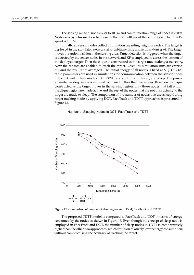
Initially, all sensor nodes collect information regarding neighbor nodes. The target isdeployed in the simulated network at an arbitrary time and in a random spot. The targetmoves in random fashion in the sensing area. Target detection is triggered when the targetis detected by the sensor nodes in the network and KF is employed to assess the location ofthe deployed target. Then the clique is constructed as the target moves along a trajectory.Now the sensors are enabled to track the target. Over 150 simulation runs are carriedout and the results are averaged. The initial energy of all nodes is fixed as 50 J. CC2420radio parameters are used in simulations for communication between the sensor nodesin the network. Three modes of CC2420 radio are transmit, listen, and sleep. The powerexpended in sleep mode is minimal compared to the other two modes. Based on the cliqueconstructed as the target moves in the sensing region, only those nodes that fall withinthe clique region are made active and the rest of the nodes that are not in proximity to thetarget are made to sleep. The comparison of the number of nodes that are asleep duringtarget tracking made by applying DOT, FaceTrack and TDTT approaches is presented inFigure 12.

Symmetry 2021, 13, x FOR PEER REVIEW 18 of 23

carried out and the results are averaged. The initial energy of all nodes is fixed as 50 J. CC2420 radio parameters are used in simulations for communication between the sensor nodes in the network. Three modes of CC2420 radio are transmit, listen, and sleep. The power expended in sleep mode is minimal compared to the other two modes. Based on the clique constructed as the target moves in the sensing region, only those nodes that fall within the clique region are made active and the rest of the nodes that are not in proxim-ity to the target are made to sleep. The comparison of the number of nodes that are asleep during target tracking made by applying DOT, FaceTrack and TDTT approaches is pre-sented in Figure 12.

Figure 12. Comparison of number of sleeping nodes in DOT, FaceTrack and TDTT.

The proposed TDTT model is compared to FaceTrack and DOT in terms of energy consumed by the nodes as shown in Figure 13. Even though the concept of sleep node is employed in FaceTrack and DOT, the number of sleep nodes in TDTT is comparatively higher than the other two approaches, which results in relatively lower energy con-sumption, without compromising the accuracy of tracking the target.

Figure 12. Comparison of number of sleeping nodes in DOT, FaceTrack and TDTT.

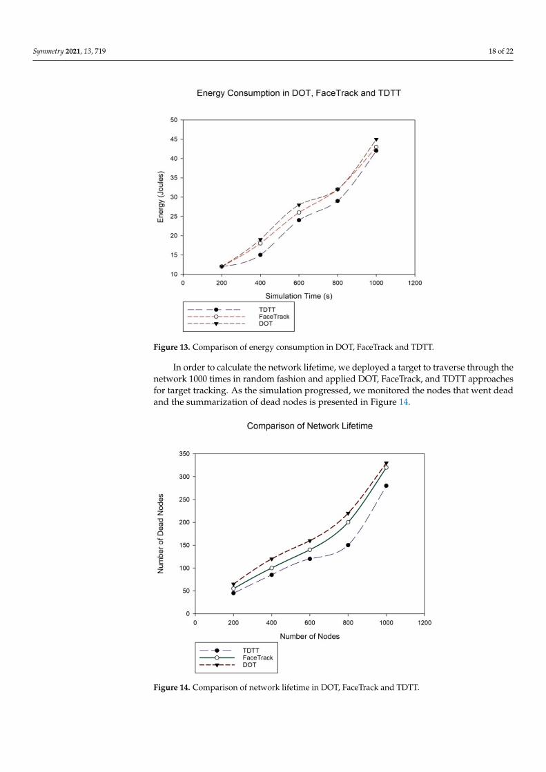
The proposed TDTT model is compared to FaceTrack and DOT in terms of energyconsumed by the nodes as shown in Figure 13. Even though the concept of sleep node isemployed in FaceTrack and DOT, the number of sleep nodes in TDTT is comparativelyhigher than the other two approaches, which results in relatively lower energy consumption,without compromising the accuracy of tracking the target.

Symmetry 2021, 13, 719 18 of 22Symmetry 2021, 13, x FOR PEER REVIEW 19 of 23

Figure 13. Comparison of energy consumption in DOT, FaceTrack and TDTT.

In order to calculate the network lifetime, we deployed a target to traverse through the network 1000 times in random fashion and applied DOT, FaceTrack, and TDTT ap-proaches for target tracking. As the simulation progressed, we monitored the nodes that went dead and the summarization of dead nodes is presented in Figure 14.

Figure 14. Comparison of network lifetime in DOT, FaceTrack and TDTT.

5.4. Comparison of TDTT with Other Existing Approaches in Terms of Accuracy In order to assess the tracking performance of TDTT, we deployed a target to trav-

erse through the network 1000 times in random fashion at random velocity range of (0, 30) m/s. Then we applied KF, EKF, DOT, FaceTrack, and TDTT approaches. The observed

Figure 13. Comparison of energy consumption in DOT, FaceTrack and TDTT.

In order to calculate the network lifetime, we deployed a target to traverse through thenetwork 1000 times in random fashion and applied DOT, FaceTrack, and TDTT approachesfor target tracking. As the simulation progressed, we monitored the nodes that went deadand the summarization of dead nodes is presented in Figure 14.

Symmetry 2021, 13, x FOR PEER REVIEW 19 of 23

Figure 13. Comparison of energy consumption in DOT, FaceTrack and TDTT.

In order to calculate the network lifetime, we deployed a target to traverse through the network 1000 times in random fashion and applied DOT, FaceTrack, and TDTT ap-proaches for target tracking. As the simulation progressed, we monitored the nodes that went dead and the summarization of dead nodes is presented in Figure 14.

Figure 14. Comparison of network lifetime in DOT, FaceTrack and TDTT.

5.4. Comparison of TDTT with Other Existing Approaches in Terms of Accuracy In order to assess the tracking performance of TDTT, we deployed a target to trav-

erse through the network 1000 times in random fashion at random velocity range of (0, 30) m/s. Then we applied KF, EKF, DOT, FaceTrack, and TDTT approaches. The observed

Figure 14. Comparison of network lifetime in DOT, FaceTrack and TDTT.

Symmetry 2021, 13, 719 19 of 22

5.4. Comparison of TDTT with Other Existing Approaches in Terms of Accuracy

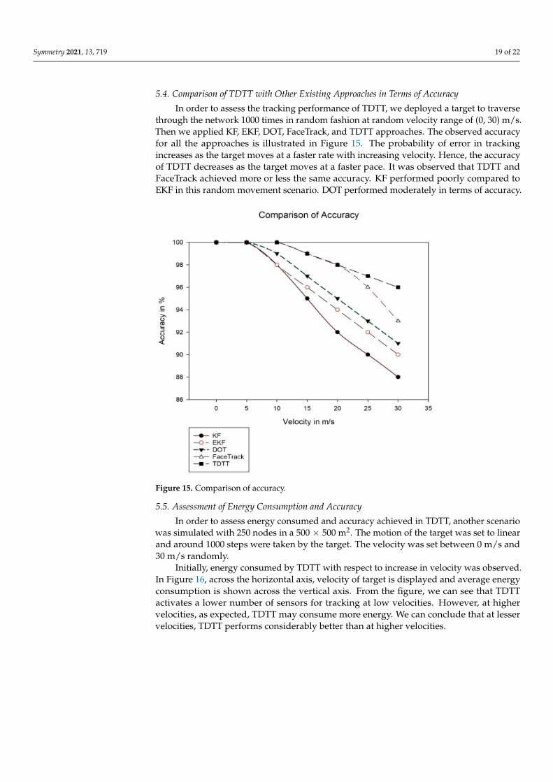
In order to assess the tracking performance of TDTT, we deployed a target to traversethrough the network 1000 times in random fashion at random velocity range of (0, 30) m/s.Then we applied KF, EKF, DOT, FaceTrack, and TDTT approaches. The observed accuracyfor all the approaches is illustrated in Figure 15. The probability of error in trackingincreases as the target moves at a faster rate with increasing velocity. Hence, the accuracyof TDTT decreases as the target moves at a faster pace. It was observed that TDTT andFaceTrack achieved more or less the same accuracy. KF performed poorly compared toEKF in this random movement scenario. DOT performed moderately in terms of accuracy.

Symmetry 2021, 13, x FOR PEER REVIEW 20 of 23

accuracy for all the approaches is illustrated in Figure 15. The probability of error in tracking increases as the target moves at a faster rate with increasing velocity. Hence, the accuracy of TDTT decreases as the target moves at a faster pace. It was observed that TDTT and FaceTrack achieved more or less the same accuracy. KF performed poorly compared to EKF in this random movement scenario. DOT performed moderately in terms of accuracy.

5.5. Assessment of Energy Consumption and Accuracy In order to assess energy consumed and accuracy achieved in TDTT, another sce-

nario was simulated with 250 nodes in a 500 × 500 m2. The motion of the target was set to linear and around 1000 steps were taken by the target. The velocity was set between 0 m/s and 30 m/s randomly.

Initially, energy consumed by TDTT with respect to increase in velocity was ob-served. In Figure 16, across the horizontal axis, velocity of target is displayed and average energy consumption is shown across the vertical axis. From the figure, we can see that TDTT activates a lower number of sensors for tracking at low velocities. However, at higher velocities, as expected, TDTT may consume more energy. We can conclude that at lesser velocities, TDTT performs considerably better than at higher velocities.

The next experiment is in regards to accuracy of TDTT at low and high velocities. Any approach would suffer from loss of accuracy at higher velocities. However, from Figure 17, we can conclude that the accuracy in TDTT at higher velocities is still adequate for the majority of applications. The association between energy saving and accuracy in various scenarios may still pose serious apprehensions. We would like to explore this association in greater depths in future work.

Figure 15. Comparison of accuracy.

Figure 15. Comparison of accuracy.

5.5. Assessment of Energy Consumption and Accuracy

In order to assess energy consumed and accuracy achieved in TDTT, another scenariowas simulated with 250 nodes in a 500 × 500 m2. The motion of the target was set to linearand around 1000 steps were taken by the target. The velocity was set between 0 m/s and30 m/s randomly.

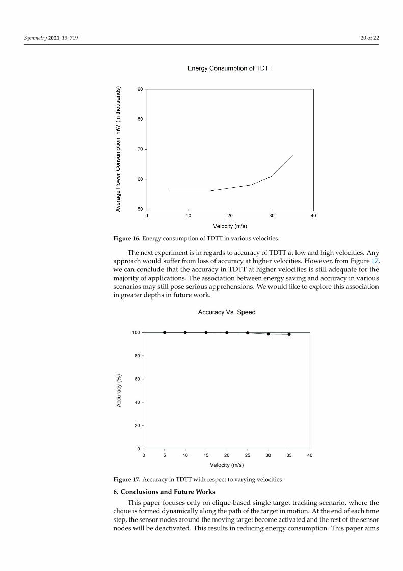
Initially, energy consumed by TDTT with respect to increase in velocity was observed.In Figure 16, across the horizontal axis, velocity of target is displayed and average energyconsumption is shown across the vertical axis. From the figure, we can see that TDTTactivates a lower number of sensors for tracking at low velocities. However, at highervelocities, as expected, TDTT may consume more energy. We can conclude that at lesservelocities, TDTT performs considerably better than at higher velocities.

Symmetry 2021, 13, 719 20 of 22Symmetry 2021, 13, x FOR PEER REVIEW 21 of 23

Figure 16. Energy consumption of TDTT in various velocities.

Figure 17. Accuracy in TDTT with respect to varying velocities.

6. Conclusions and Future Works This paper focuses only on clique-based single target tracking scenario, where the

clique is formed dynamically along the path of the target in motion. At the end of each time step, the sensor nodes around the moving target become activated and the rest of

Figure 16. Energy consumption of TDTT in various velocities.

The next experiment is in regards to accuracy of TDTT at low and high velocities. Anyapproach would suffer from loss of accuracy at higher velocities. However, from Figure 17,we can conclude that the accuracy in TDTT at higher velocities is still adequate for themajority of applications. The association between energy saving and accuracy in variousscenarios may still pose serious apprehensions. We would like to explore this associationin greater depths in future work.

Symmetry 2021, 13, x FOR PEER REVIEW 21 of 23

Figure 16. Energy consumption of TDTT in various velocities.

Figure 17. Accuracy in TDTT with respect to varying velocities.

6. Conclusions and Future Works This paper focuses only on clique-based single target tracking scenario, where the

clique is formed dynamically along the path of the target in motion. At the end of each time step, the sensor nodes around the moving target become activated and the rest of

Figure 17. Accuracy in TDTT with respect to varying velocities.

6. Conclusions and Future Works

This paper focuses only on clique-based single target tracking scenario, where theclique is formed dynamically along the path of the target in motion. At the end of each timestep, the sensor nodes around the moving target become activated and the rest of the sensornodes will be deactivated. This results in reducing energy consumption. This paper aims

Symmetry 2021, 13, 719 21 of 22

to detect and track a target with maximum accuracy and minimum energy consumptionin each sensor node. TDTT uses KF for target detection and clique-based estimation fortracking the target. The results are found to be encouraging. We implemented DOT andface-based tracking approach for comparison with TDTT.

The experimental results prove that employing TDTT improves energy efficiency andextends the lifetime of the network without compromising the accuracy of tracking. Thismodel could be experimented on with multiple targets, as tracking multiple targets posesserious difficulty in associating the trajectory with individual targets in the sensing region.

Author Contributions: Conceptualization, P.L.R. and G.A.S.K.; methodology, P.L.R.; software, P.L.R.;validation, P.L.R. and G.A.S.K.; formal analysis, P.L.R.; investigation, P.L.R.; resources, P.L.R.; datacuration, P.L.R.; writing—original draft preparation, P.L.R.; writing—review and editing, G.A.S.K.;visualization, G.A.S.K.; supervision, G.A.S.K. Both authors have read and agreed to the publishedversion of the manuscript.

Funding: This research received no external funding.

Institutional Review Board Statement: Not applicable.

Conflicts of Interest: The authors declare no conflict of interest.

References1. Barile, G.; Leoni, A.; Pantoli, L.; Stornelli, V. Real-time autonomous system for structural and environmental monitoring of

dynamic events. Electronics 2018, 7, 420. [CrossRef]2. Zhao, F.; Shin, J.; Reich, J. Information-driven dynamic sensor collaboration. IEEE Signal Process. Mag. 2002, 19, 61–72. [CrossRef]3. Lau, E.E.L.; Chung, W.Y. Enhanced RSSI-Based Real-Time User Location Tracking System for Indoor and Outdoor Environments.

In Proceedings of the 2007 International Conference on Convergence Information Technology (ICCIT 2007), Gyeongju-si, Korea,21–23 November 2007.

4. Kumar, S.; Hegde, R.M. A Review of Localization and Tracking Algorithms in Wireless Sensor Networks 2017. Available online:http://arxiv.org/abs/1701.02080 (accessed on 9 January 2017).

5. Viani, F.; Rocca, P.; Oliveri, G.; Trinchero, D.; Massa, A. Localization, tracking, and imaging of targets in wireless sensor networks:An invited review. Radio Sci. 2011, 46, RS5002. [CrossRef]

6. Catovic, A.; Sahinoglu, Z. The Cramer-Rao bounds of hybrid TOA/RSS and TDOA/RSS location estimation schemes. IEEECommun. Lett. 2004, 8, 626–628. [CrossRef]

7. Vasuhi, S.; Vaidehi, V. Target tracking using interactive multiple model for wireless sensor network. Inf. Fusion 2016, 27, 41–53.[CrossRef]

8. Cheng, L.; Wang, Y.; Sun, X.; Hu, N.; Zhang, J. A mobile localization strategy for wireless sensor network in NLOS conditions.China Commun. 2016, 13, 69–78. [CrossRef]

9. Mahfouz, S.; Mourad-Chehade, F.; Honeine, P.; Farah, J.; Snoussi, H. Target tracking using machine learning and kalman filter inwireless sensor networks. IEEE Sens. J. 2014, 14, 3715–3725. [CrossRef]

10. Souza, E.L.; Nakamura, E.F.; Pazzi, R.W. Target tracking for sensor networks: A survey. ACM Comput. Surv. 2016, 49. [CrossRef]11. Pahlavan, K.; Li, X. Indoor geolocation science and technology. IEEE Commun. Mag. 2002, 40, 112–118. [CrossRef]12. Ashraf, I.; Hur, S.; Park, Y. Indoor Positioning on Disparate Commercial Smartphones Using Wi-Fi Access Points Coverage Area.

Sensors 2019, 19, 4351. [CrossRef]13. Ali, M.U.; Hur, S.; Park, S.; Park, Y. Harvesting Indoor Positioning Accuracy by Exploring Multiple Features From Received

Signal Strength Vector. IEEE Access 2019, 7, 52110–52121. [CrossRef]14. Patwari, N.; Wilson, J. RF sensor networks for device-free localization: Measurements, models, and algorithms. Proc. IEEE 2010,

99, 1–13. [CrossRef]15. Wilson, J.; Patwari, N. See through walls: Motion tracking using variance-based radio tomography networks. IEEE Trans. Mobile

Comput. 2011, 10, 612–621. [CrossRef]16. Touvat, F.; Poujaud, J.; Noury, N. Indoor localization with wearable RF devices in 868 MHz and 2.4 GHz bands. In Proceedings of

the IEEE 16th International Conference on e-Health Networking, Applications and Services (Healthcom), Natal, Brazil, 15–18October 2014; pp. 136–139.

17. Bosisio, A.V. Performances of an RSSI-based positioning and tracking algorithm. In Proceedings of the Indoor Positioning andIndoor Navigation (IPIN), 2011 International Conference, Guimarães, Portugal, 21–23 September 2011; pp. 1–8. [CrossRef]

18. Leela Rani, P.; Sathish Kumar, G.A. A survey on algorithms used for tracking targets in WSNs. In Proceedings of the 2017International Conference on Energy, Communication, Data Analytics and Soft Computing (ICECDS), Chennai, India, 1–2 August2017; pp. 1464–1468. [CrossRef]

19. Sadowski, S.; Spachos, P. RSSI-Based Indoor Localization with the Internet of Things. IEEE Access 2018, 6, 30149–30161. [CrossRef]

Symmetry 2021, 13, 719 22 of 22

20. Ceylan, O.; Taraktas, K.F.; Yagci, H.B. Enhancing RSSI Technologies in Wireless Sensor Networks by Using Different Frequencies.In Proceedings of the 2010 International Conference on Broadband, Wireless Computing, Communication and Applications,Fukuoka, Japan, 4–6 November 2010; pp. 369–372. [CrossRef]

21. Ahmadi, H.; Viani, F.; Polo, A.; Bouallegue, R. Improved target tracking using regression tree in wireless sensor networks. InProceedings of the 2016 IEEE/ACS 13th International Conference of Computer Systems and Applications (AICCSA), Agadir,Morocco, 29 November–2 December 2016; pp. 1–6.

22. Jondhale, S.R.; Deshpande, R.S.; Walke, S.M.; Jondhale, A.S. Issues and challenges in RSSI based target localization and tracking inwireless sensor networks. In Proceedings of the 2016 International Conference on Automatic Control and Dynamic OptimizationTechniques (ICACDOT), Pune, India, 9–10 September 2016; pp. 594–598. [CrossRef]

23. Din, S.; Paul, A.; Ahmad, A.; Kimet, J.H. Energy efficient topology management scheme based on clustering technique forsoftware defined wireless sensor network. Peer-to-Peer Netw. Appl. 2019, 12, 348–356. [CrossRef]

24. Sthapit, P.; Gang, H.; Pyun, J. Bluetooth Based Indoor Positioning Using Machine Learning Algorithms. In Proceedings of the 2018IEEE International Conference on Consumer Electronics-Asia (ICCE-Asia), JeJu, Korea, 24–26 June 2018; pp. 206–212. [CrossRef]

25. Banihashemian, S.S.; Adibnia, F.; Sarram, M.A. A New Range-Free and Storage-Efficient Localization Algorithm Using NeuralNetworks in Wireless Sensor Networks. Wireless Pers. Commun. 2018, 98, 1547–1568. [CrossRef]

26. Kalman, R.E.; Bucy, R.S. A new approach to linear filtering and prediction problems. Trans. ASME J. Basic Eng. ASME 1960, 82D,34–45. [CrossRef]

27. Giannitrapani, A.; Ceccatrlli, N.; Scortecci, F.; Garulli, A. Comparison of EKF and UKF for Spacecraft Localization via AngleMeasurements. IEEE Trans. Aerosp. Electron. Syst. 2011, 47, 75–84. [CrossRef]

28. Fayazi Barjini, E.; Gharavian, D.; Shahgholian, M. Target tracking in wireless sensor networks using NGEKF algorithm. J. AmbientIntell. Human Comput. 2020, 11, 3417–3429. [CrossRef]

29. Jondhale, S.R.; Deshpande, R.S. Kalman Filtering Framework-Based Real Time Target Tracking in Wireless Sensor NetworksUsing Generalized Regression Neural Networks. IEEE Sens. J. 2019, 19, 224–233. [CrossRef]

30. Chuang, P.-J.; Jiang, Y. Effective neural network-based node localisation scheme for wireless sensor networks. IET Wirel. Sens.Syst. 2014, 4, 97–103. [CrossRef]

31. Torres-Sospedra, J.; Montoliu, R.; Martínez-Usó, A.; Avariento, J.P.; Arnau, T.J.; Benedito-Bordonau, M.; Huerta, J. Ujiindoorloc: Anew multi-building and multi floor database for WLAN finger print based indoor localization problem. In Proceedings of the 2014International Conference on Indoor Positioning and Indoor Navigation (IPIN), Busan, Korea, 27–30 October 2014; pp. 261–270.

32. Ali, K.; Rasid, M.F.A.; Sali, A. Face-Based Mobile Target Tracking Technique in Wireless Sensor Network. Wirel. Pers. Commun.2020, 111, 1853–1870. [CrossRef]

33. Tsai, H.-W.; Chu, C.-P.; Chen, T.-S. Mobile object tracking in wireless sensor networks. Comput. Commun. 2007, 30, 1811–1825.[CrossRef]

34. Wang, G.; Bhuiyan, M.; Cao, J.; Wu, J. Detecting movements of a target using face tracking in wireless sensor networks. IEEETrans. Parallel Distrib. Syst. 2014, 25, 1–11. [CrossRef]

35. Javed, N.; Wolf, T. Multiple object tracking in sensor networks using distributed clique finding. In Proceedings of the 2013International Conference on Computing, Networking and Communications (ICNC), San Diego, CA, USA, 28–31 January 2013;pp. 1139–1145. [CrossRef]