Design of the Audio Coding Standards for MPEG and AC-3 · Design of the Audio Coding Standards for MPEG and AC-3 ... ISO MPEG 1/2 and Dolby AC-3 are ... adaptive filterbank, and psychoacoustic

1

Design of the Audio Coding Standards for MPEG and AC-3

Student Wen-Chieh Lee Advisor Dr. Chi-Min Liu

Institute of Computer Science and Information Engineering

National Chiao-Tung University

ABSTRACT

ISO MPEG 1/2 and Dolby AC-3 are widely used in the network, wireless,

multimedia system and video industry. This dissertation studies the design of

audio standards: MPEG-1/2 and AC-3.

The perceptual audio coder like MPEG-1/2 and AC-3 can be analyzed

through filterbank, psychoacoustic model, stereo matrix, bit allocation/

quantization, and packing block. This dissertation considers the design for the

filterbank, psychoacoustic model, stereo matrix, and bit allocation/ quantization.

This dissertation summarizes the filterbanks adopted in coding standards and

presents a unified fast algorithm for these filter banks. On the psychoacoustic

models, the hybrid filterbank is proposed to replace to original frequency

analyzer for MPEG audio standards to have efficient computing. On the bit

allocation, we analyze the issues in bit allocation and present the efficient

method. This dissertation also studies the stereo irrelevancy and presents the

new method to achieve good quality.

Keywords: MPEG, AC-3, Audio coding, Filterbank, Bit allocation,

Intensity/coupling coding, Layer 3.

2

Contents

List of Tables........................................................................................................5

List of Figures ......................................................................................................7

Chapter 1 Introduction.................................................................................... 10

Chapter 2 Unified Algorithm for Fast Filterbank Computing.................... 15

2.1 Introduction ................................................................................. 15

2.2 Unified Form for the CMFBS ..................................................... 19

2.2.1 Unified form for the MCT in TDAC filterbank ................... 21

2.2.2 Unified form for the variant of TDAC filterbanks ............... 29

2.2.3 Unified form for the polyphase filterbank............................ 32

2.3 Fast Algorithm for the Discrete Cosine Transform..................... 37

2.3.1 Decomposition for type-II DCT ........................................... 37

2.3.2 Decomposition for type-III DCT.......................................... 39

2.3.3 Decomposition for type-IV DCT.......................................... 41

2.4 Concluding Remarks ................................................................... 44

Chapter 3 Fast Frequency Analysis for the Psychoacoustic Model ............ 47

3.1 Introduction ................................................................................. 47

3.2 Hybrid Filterbank for Psychoacoustic Model in MPEG ............. 48

3.2.1 Filter response in hybrid filterbanks..................................... 50

3.2.2 Phase shifter & alias reduction ............................................. 53

3

3.2.3 Complexity analysis.............................................................. 57

3.2.4 Cooperating with the intensity mode.................................... 58

3.2.5 Tonality measure .................................................................. 59

3.2.6 Effects of the hybrid filterbank and quality measurement ... 61

3.3 Concluding Remarks ................................................................... 64

Chapter 4 Fast Bit Allocation Method ........................................................... 65

4.1 Introduction ................................................................................. 67

4.2 Fast Bit Allocation Method in MPEG Layer 3............................ 68

4.2.1 Noise predictor for non-uniform quantizer........................... 70

4.2.2 Fast bit allocation for non-uniform quantizer....................... 75

4.3 Fast Bit Allocation Method in AC-3 ........................................... 79

4.3.1 Addressed issues................................................................... 79

4.3.2 Exponent coding method ...................................................... 82

4.3.3 Perceptual parameters........................................................... 84

4.3.4 Experiment results ................................................................ 89

4.3.5 Remarks ................................................................................ 90

4.4 Concluding Remarks ................................................................... 92

Chapter 5 KL Transform for Intensity/Coupling Coding ........................... 93

5.1 Introduction ................................................................................. 93

5.2 KL Transform for AC-3 .............................................................. 94

5.2.1 Addressed issues................................................................... 95

5.2.2 Four proposed coupling methods ......................................... 97

5.2.3 Experiments on the coupling methods ............................... 103

4

5.2.4 Dithering on the coupling bands......................................... 105

5.2.5 Remarks .............................................................................. 105

5.3 KL Transform for MPEG Intensity Coding [6]......................... 107

5.4 Concluding Remarks ................................................................. 111

Chapter 6 Conclusions and Future Works .................................................. 112

6.1 Concluding Remarks ................................................................. 112

6.2 Future Works ............................................................................. 113

Bibliography 115

Curriculum Vita ............................................................................................. 120

Publication Lists ............................................................................................. 121

5

List of Tables

Table 1.1 Audio coding standards and applications. ..............................................................12

Table 2.1 The formulae and the classification of the CMFBs in current audio coding standards.

................................................................................................................................45

Table 2.2 Arithmetic operations required in the fast algorithms of DCTs where Op stands for

the arithmetic operations required for the row, where x denotes multiplication

operation while + addition operation. The 2, 4, 8, 16, 32, and 64 in first column

denote the transform length. The entries of the row associating with the transform

length illustrate the operations required for the algorithm labeled in the entry of the

first row of the column. ..........................................................................................45

Table 3.1 Audio standards and frequency analysis in psychoacoustic model........................48

Table 3.2 Eight weighting factors of alias reduction butterfly. ..............................................57

Table 3.3 Complexity comparison between FFT and hybrid filterbank.................................58

Table 4.1 Noise estimation and bit allocation scheme in audio standards .............................70

Table 4.2 Average iteration number for different testing material for the proposed and MPEG

bit allocation algorithm...........................................................................................79

Table 4.3 Average iteration counts per frame. .......................................................................89

Table 4.4 Candidates of exponent coding strategies. .............................................................90

Table 5.1 A summary of stereo matrix mechanism among audio standards. .........................94

Table 5.2 Testing audio segments and their descriptions.......................................................106

6

Table 5.3 NMRseg values for the four proposed coupling methods under high bit rate with D15

mode 6 times per frame. .........................................................................................106

Table 5.4 NMRseg values for the four proposed coupling methods under the bit rate of 128

kbits/sec with D15 mode once per frame. ..............................................................107

Table 5.5 MNR (dB) values in layer 2. In each box, the upper value is for the left channel, the

lower value is for the right channel (adopted from [6]). ........................................110

7

List of Figures

Fig. 1.1 Block diagram for perceptual audio coder. ...............................................................14

Fig. 2.1 The cosine-modulated filterbanks in the audio encoder and the decoder. ................17

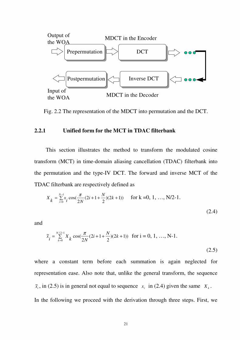
Fig. 2.2 The representation of the MDCT into permutation and the DCT. ............................21

Fig. 2.3 The decomposition of one 8-point type-II DCT into one 4-point type-II DCT and one

4-point type-IV DCT. .............................................................................................39

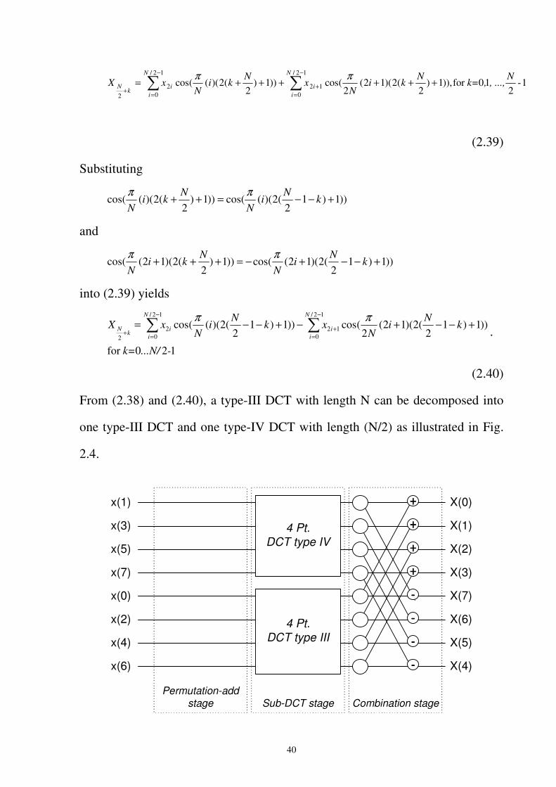
Fig. 2.4 The decomposition of one 8-point type-III DCT into one 4-point type-III DCT and

one 4-point type-IV DCT. ......................................................................................41

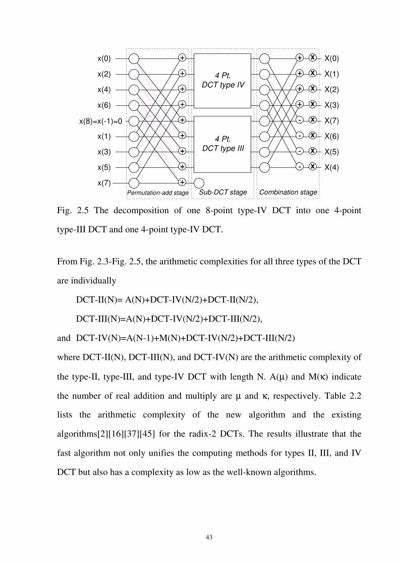
Fig. 2.5 The decomposition of one 8-point type-IV DCT into one 4-point type-III DCT and

one 4-point type-IV DCT. ......................................................................................43

Fig. 3.1 The Structure of the FFT-based MPEG Encoder ......................................................49

Fig. 3.2 Structure of MPEG encoder based on the hybrid filterbanks ...................................51

Fig. 3.3 Detailed structure of the hybrid filterbank ................................................................52

Fig. 3.4 Power spectrum of the 2nd level filterbank................................................................53

Fig. 3.5 Alias in neighboring subbands ..................................................................................55

Fig. 3.6 Structure of alias reduction butterfly.........................................................................56

Fig. 3.7 Hybrid filterbank resolution vs. critical band............................................................58

Fig. 3.8 Conventional intensity stereo coding scheme ...........................................................60

Fig. 3.9 Intensity stereo coding through the hybrid-based psychoacoustic model.................61

8

Fig. 3.10 Signal with frequency located at 400Hz, 800Hz, 1600Hz, 3200Hz and 6400Hz

analyzed by 1024 pt. FT (dotted line), the hybrid filterbank (dashed line) and the

hybrid filterbank with alias reduction butterfly (solid line) ...................................62

Fig. 3.11 Average signal-to-masking ratio of each subband for female vocal sound. ...........63

Fig. 3.12 Average signal-to-masking ratio of each subband for classical symphony orchestra.

................................................................................................................................63

Fig. 3.13 Average signal-to-masking ratio of each subband for high frequency tone at 12 Hz.

................................................................................................................................63

Fig. 4.1 The relation of optimal noise shaping for different bit rate for Noise 1 and Noise 2

with Signalk and Maskingk......................................................................................67

Fig. 4.2 Relation of noise estimator and quantizer in ABS scheme. ......................................69

Fig. 4.3 Relation of noise estimator and quantizer in predictor scheme. ...............................70

Fig. 4.4 Non-uniform quantizer in MPEG layer 3, where step size as (4.3),

)(43

2 sfbgr scalegainsfb

−=∆ ..........................................................................................72

Fig. 4.5 Signal-to-masking ratio (SMR) and signal-to-noise ratio (SNR) curve. Solid line is

the SMR value; long slash line is the SNR value for original bit allocation; short

slash line is the SNR value for new bit allocation algorithm under 128 kbit/s. .....78

Fig. 4.6 Encoding process for AC-3. ......................................................................................81

Fig. 4.7 Block diagram of exponent coding process. .............................................................84

Fig. 4.8 Modeling spreading function. ...................................................................................85

Fig. 4.9 Flowchart of mantissa quantization...........................................................................87

Fig. 4.10 Block diagram of the quantization parameter search. .............................................88

Fig. 4.11 Frequency responses of three typical audio sequences, where the lowest curve is

encoded by D15, the middle curve by D25 and the highest curve by D45. ...........91

9

Fig. 5.1 Block diagram of the coupling process in a coupling band of the Dolby AC-3 codec.

................................................................................................................................96

Fig. 5.2 The SUM algorithm for the coupling process...........................................................102

Fig. 5.3 The NORM_SUM algorithm for the coupling process.............................................102

Fig. 5.4 The KLT_MSE algorithm for the coupling process. ................................................103

Fig. 5.5 The KLT_ENG algorithm for the coupling process. ................................................103

Fig. 5.6 Intensity stereo coding of MPEG-1 (SUM) in a high frequency band (adopted from

[6]). .........................................................................................................................108

Fig. 5.7 KL_MSE intensity coding in a high frequency band (adopted from [6]). ................110

10

Chapter 1 Introduction

During the last decade, analog audio has been wholly replaced by the

CD-quality digital audio. The demand for digital audio compression with

constraint bandwidth, limit storage is rapidly increased for the network, wireless,

multimedia system and video industry. In response to this need, considerable

researches for the perceptually transparent coding of high-fidelity (CD-quality)

digital audio have been developed. Several algorithms have now become

international standards or commercial products. ISO MPEG-1/2 layer 1/2/3 and

Dolby AC-3 are the most widely adopted among the standards such as- HDTV,

DVD, VCD, and Internet audio.

MPEG-1 [24] comprises a flexible hybrid coding technique that

incorporates several methods including subband decomposition, filterbank

analysis, transform coding, entropy coding, dynamic bit allocation, non-uniform

quantization, adaptive filterbank, and psychoacoustic analysis. MPEG coders

accept 16-bit PCM input data at sample rates of 32, 44.1, and 48 kHz. MPEG-1

offers separate modes for mono, stereo, dual independent mono, and joint stereo.

Available bit rates are 32-192 kb/s for mono and 64-384 kb/s for stereo.

The MPEG layer 3 achieves quality improvements by adding several

important mechanisms on the foundation of the layer 1/2. A hybrid filterbank is

11

introduced to increase frequency resolution and thereby better approximate

critical band behavior. The hybrid filterbank includes adaptive filterbank to

improve pre-echo control. Sophisticated bit allocation and quantization

strategies that rely upon non-uniform quantization, analysis–by-synthesis, and

entropy coding are introduced to allow reduced bit rates and improved quality.

First, a hybrid filterbank is constructed by following each subband filter with an

adaptive MDCT. This practice allows for higher frequency resolution and

pre-echo control. Use of an 18- point MDCT, for example, improves frequency

resolution to 41.67 Hz per spectral line. Adaptive MDCT block sizes between 6

and 18 points allow improved pre-echo control. Using shorter blocks during

rapid attacks in the input sequence allows pre-masking to hide pre-echoes, while

using longer blocks during steady-state periods reduces side information and

hence bit rates. Bit allocation and quantization of the spectral lines is realized in

a nested loop procedure that uses both non-uniform quantization and Huffman

coding. The inner loop adjusts the non-uniform quantizer step sizes for each

block until the number of bits required to encode the transform components falls

within the bit budget. The outer loop evaluates the quality of the coded signal

(analysis-by-synthesis) in terms of quantization noise relative to the JND

thresholds.

MPEG-2 [23] extends the capabilities offered by MPEG-1 to support the so

called 3/2 channel format with left, right, center, and left and right surround

channels. The first MPEG-2 standard is backward compatible with MPEG-1 in

the sense that 3/2 channel information transmitted by an MPEG-2 encoder can

be correctly decoded for 2-channel presentation by an MPEG-1 receiver. The

12

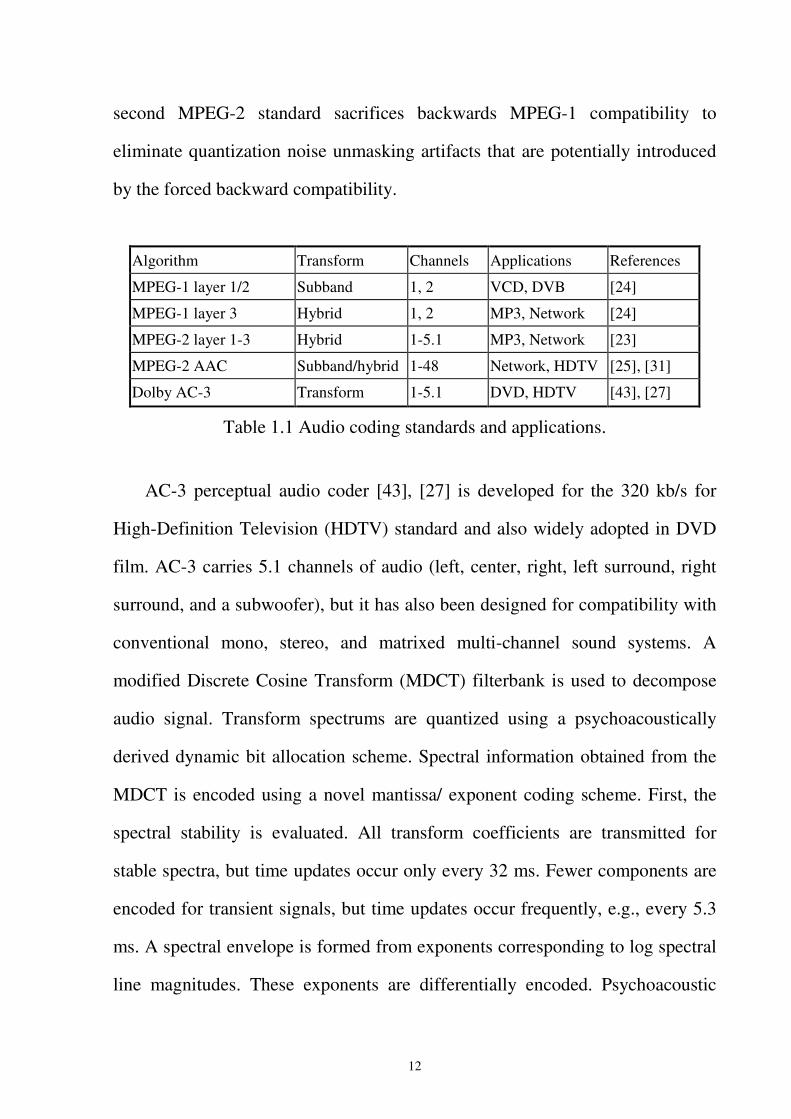
second MPEG-2 standard sacrifices backwards MPEG-1 compatibility to

eliminate quantization noise unmasking artifacts that are potentially introduced

by the forced backward compatibility.

Algorithm Transform Channels Applications References

MPEG-1 layer 1/2 Subband 1, 2 VCD, DVB [24]

MPEG-1 layer 3 Hybrid 1, 2 MP3, Network [24]

MPEG-2 layer 1-3 Hybrid 1-5.1 MP3, Network [23]

MPEG-2 AAC Subband/hybrid 1-48 Network, HDTV [25], [31]

Dolby AC-3 Transform 1-5.1 DVD, HDTV [43], [27]

Table 1.1 Audio coding standards and applications.

AC-3 perceptual audio coder [43], [27] is developed for the 320 kb/s for

High-Definition Television (HDTV) standard and also widely adopted in DVD

film. AC-3 carries 5.1 channels of audio (left, center, right, left surround, right

surround, and a subwoofer), but it has also been designed for compatibility with

conventional mono, stereo, and matrixed multi-channel sound systems. A

modified Discrete Cosine Transform (MDCT) filterbank is used to decompose

audio signal. Transform spectrums are quantized using a psychoacoustically

derived dynamic bit allocation scheme. Spectral information obtained from the

MDCT is encoded using a novel mantissa/ exponent coding scheme. First, the

spectral stability is evaluated. All transform coefficients are transmitted for

stable spectra, but time updates occur only every 32 ms. Fewer components are

encoded for transient signals, but time updates occur frequently, e.g., every 5.3

ms. A spectral envelope is formed from exponents corresponding to log spectral

line magnitudes. These exponents are differentially encoded. Psychoacoustic

13

quantization masking thresholds are derived from the decoded spectral envelope

for 64 non-uniform subbands that increase in size proportional to the ear’s

critical bands. The thresholds are used to select appropriate quantizers for

transform coefficient mantissas in a bit allocation loop. If too few bits are

available, high-frequency coupling (above 2 kHz) between channels may be

used to reduce the amount of transmitted information. Exponents, mantissas,

coupling data, and exponent strategy data are combined and transmitted.

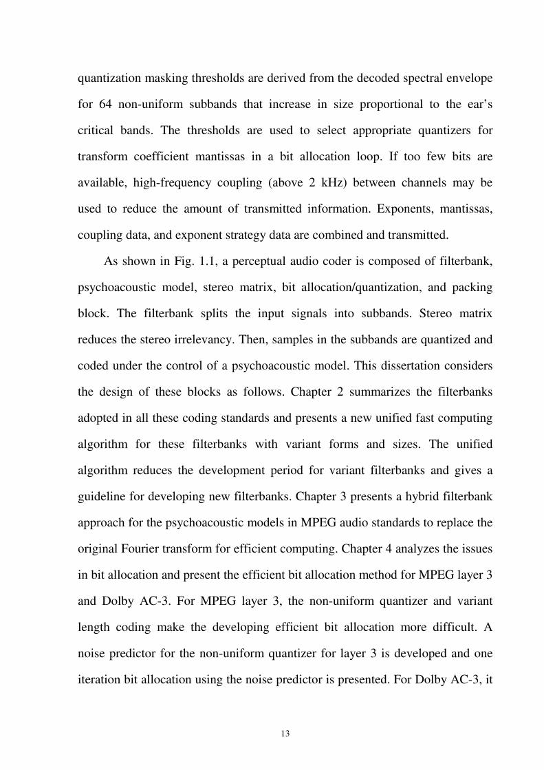
As shown in Fig. 1.1, a perceptual audio coder is composed of filterbank,

psychoacoustic model, stereo matrix, bit allocation/quantization, and packing

block. The filterbank splits the input signals into subbands. Stereo matrix

reduces the stereo irrelevancy. Then, samples in the subbands are quantized and

coded under the control of a psychoacoustic model. This dissertation considers

the design of these blocks as follows. Chapter 2 summarizes the filterbanks

adopted in all these coding standards and presents a new unified fast computing

algorithm for these filterbanks with variant forms and sizes. The unified

algorithm reduces the development period for variant filterbanks and gives a

guideline for developing new filterbanks. Chapter 3 presents a hybrid filterbank

approach for the psychoacoustic models in MPEG audio standards to replace the

original Fourier transform for efficient computing. Chapter 4 analyzes the issues

in bit allocation and present the efficient bit allocation method for MPEG layer 3

and Dolby AC-3. For MPEG layer 3, the non-uniform quantizer and variant

length coding make the developing efficient bit allocation more difficult. A

noise predictor for the non-uniform quantizer for layer 3 is developed and one

iteration bit allocation using the noise predictor is presented. For Dolby AC-3, it

14

adapts its range according to the specified exponent strategy. These strategies

affect the temporal resolution and the spectral resolution of the quantization

ranges. These encoded exponents also affect the analysis result of the

psychoacoustic model. The exponents and the resultant psychoacoustic results

determine the quantization results and thus has led to high complexity. This

dissertation present the criteria to decide the strategies for the exponent coding

and psychoacoustic model parameter and propose a efficient bit allocation

algorithm for AC-3. Chapter 5 studies the stereo irrelevancy and presents the

design method. KL (Karhunen-Loève) transform is introduced to design and

analyze the intensity/coupling schemes to reduce stereo irrelevancy. With

integrating the KL transform into intensity coding/coupling schemes of MPEG

and AC-3, this dissertation presents and compares the algorithms to improve

quality. Chapter 6 concludes the dissertation.

Audio in Filterbank Stereo

matrix

Bit allocation

Psychoacoustic model

Quantization & pack

Fig. 1.1 Block diagram for perceptual audio coder.

15

Chapter 2 Unified Algorithm for Fast Filterbank Computing

Current audio coding standards such as MPEG-1 layers 1-3, MPEG-2

layers 1-4, MPEG-4, and AC-3, have adopted for compression various forms of

the filterbank (CMFBs). This chapter demonstrates that all these MCTs can be

derived into two modules: the permutation and the discrete cosine transform.

The derived DCTs are either type-II, type-III, or type IV. On the three types of

the DCT, this chapter proposes a fast computing algorithm to uniformly

compute all the three types of the DCTs. The new fast algorithm has good

features in regularity, complexity, and general applicability.

2.1 Introduction

In current audio coding standards such as MPEG-1 layers 1-3, MPEG-2

layers 1-4, MPEG-4, and AC-3, the cosine-modulated filterbanks (CMFBs) [41]

have been widely adopted to transform an audio sequence from time-domain to

transform domain or subband domain for compression. However, all the

CMFBs’ formulae vary with not only the standards but also with the standard

layers, block length, encoding, and decoding process. For real-time applications,

16

these various formulae need to be individually designed and tuned for precision,

complexity, and memory movements. This chapter will develop the unified fast

algorithm for these formulae.

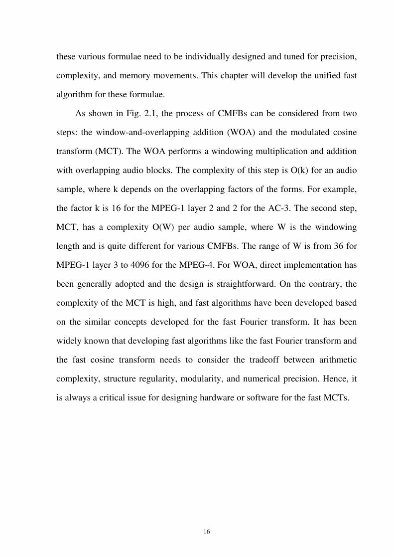
As shown in Fig. 2.1, the process of CMFBs can be considered from two

steps: the window-and-overlapping addition (WOA) and the modulated cosine

transform (MCT). The WOA performs a windowing multiplication and addition

with overlapping audio blocks. The complexity of this step is O(k) for an audio

sample, where k depends on the overlapping factors of the forms. For example,

the factor k is 16 for the MPEG-1 layer 2 and 2 for the AC-3. The second step,

MCT, has a complexity O(W) per audio sample, where W is the windowing

length and is quite different for various CMFBs. The range of W is from 36 for

MPEG-1 layer 3 to 4096 for the MPEG-4. For WOA, direct implementation has

been generally adopted and the design is straightforward. On the contrary, the

complexity of the MCT is high, and fast algorithms have been developed based

on the similar concepts developed for the fast Fourier transform. It has been

widely known that developing fast algorithms like the fast Fourier transform and

the fast cosine transform needs to consider the tradeoff between arithmetic

complexity, structure regularity, modularity, and numerical precision. Hence, it

is always a critical issue for designing hardware or software for the fast MCTs.

17

WOAWOA MCTMCT

WOAWOA Inverse MCTInverse MCT

CMFB process in Encoder

CMFB process in Decoder

AudioInput

AudioOutput

Fig. 2.1 The cosine-modulated filterbanks in the audio encoder and the decoder.

As illustrated in Fig. 2.1, this section demonstrates that all the various

MCTs can be derived into two modules: the pre- (or post-) permutation and the

discrete cosine transform (DCT). The DCT derived from the MCTs can be one

of the three types of DCTs generally referred to as type-II, type-III, and type-IV

[34]. On the results, this chapter further develops a fast algorithm which

recursively decomposes a type of DCT with length N into other types of DCTs

with length N/2. Recursive decomposition is the vehicle adopted in developing

fast algorithms for sinusoidal transforms such as the discrete Fourier transform

and the discrete cosine transforms. However, the main difference of the

recursive decomposition is the decomposition of one type of DCT into type-II,

type-III, or type-IV. The difference leads to two important benefits. First, the

approach has a data regularity that is a property of the fast Fourier transform but

not for the fast cosine transform. The regularity is important for the data path

design in VLSI chip design [5], [22] and the memory addressing in software

programming. The second merit is that the fast algorithm can be optimally

implemented for all the MCTs in audio standards. Since this algorithm

18

recursively and regularly decomposes the long length transforms into short

length ones through three types of the DCTs, the unrolling of the recursive

decomposition from length N into length 2 will be the interleaving of the three

types of the DCTs. In other word, the fast algorithm is applicable to all the three

types of the DCT, and the computing vehicle for the three DCT types is the

same. Hence, this section demonstrates that all the various CMFBs in the audio

coding standards lead to different pre-permutation or post-permutation but will

have the same computing vehicle for the DCTs. Through the same computing

vehicle, the software modules or hardware modules can be generally developed

for all these audio compression standards.

There have been many fast computing algorithms developed for the DCT. These

algorithms are developed for different transform length and different DCT types.

On the audio coding, radix-2 DCT is the main considering length. The

development of the radix-2 fast DCT algorithms can be classified into two

approaches: (1) the indirect computation of the DCT through the fast Fourier

transform or the fast Hartley transform, and (2) the direct computation of the

DCT through matrix factorization or recursive decomposition. The first

approach needs additional complexity in mapping DCTs into another transform

while the second approach in general lacks the modularity and data regularity.

As mentioned by Yun [20], the modularity and the regularity are essential for

designing hardware and generalizing to higher order transforms. Recently, Kok

[16] has developed a fast algorithm for type-II DCT that can recursively

decomposes one type-II DCT with length N into two type-II DCTs with length

(N/2). The decomposition from one DCT into two DCTs leads to the merit in

19

modularity and regularity. This section adopts the direct computation approach

to achieve low complexity. The complexity analysis shows that the new

algorithm can have a complexity matching with the well-known DCT algorithm

[16][2][45][37]. Furthermore, we develop the decomposition through the

interleaving of three types of DCTs instead of the same type of DCT to improve

the regularity and the modularity. Since the decomposition is the interleaving of

the three types of the DCTs, the fast algorithm is applicable to all three types of

the DCTs instead of just the type II in [16]. The general applicability is the key

factor to develop the fast algorithm for the cosine-modulated filterbanks

(CMFBs) in the current audio standards.

The rest of this chapter is organized as follows: Section 2.2 illustrates that

all the CMFBs can be derived into permutation and the discrete cosine transform.

Section 2.3 demonstrates the decomposition of one type of the DCT into the

interleaving of the other three DCT types to achieve fast computing. Section 2.4

gives concluding remarks.

2.2 Unified Form for the CMFBS

The modulated cosine transforms (MCTs) used in current audio standards

can be classified into three types of filterbanks: the time-domain aliasing

cancellation (TDAC) filterbank [30], the variant of the TDAC filterbank [43],

and the polyphase filterbank [24]. Table 2.1 illustrates the formulae of the three

classes of the cosine-modulated filterbanks (CMFBs) and the correspondence

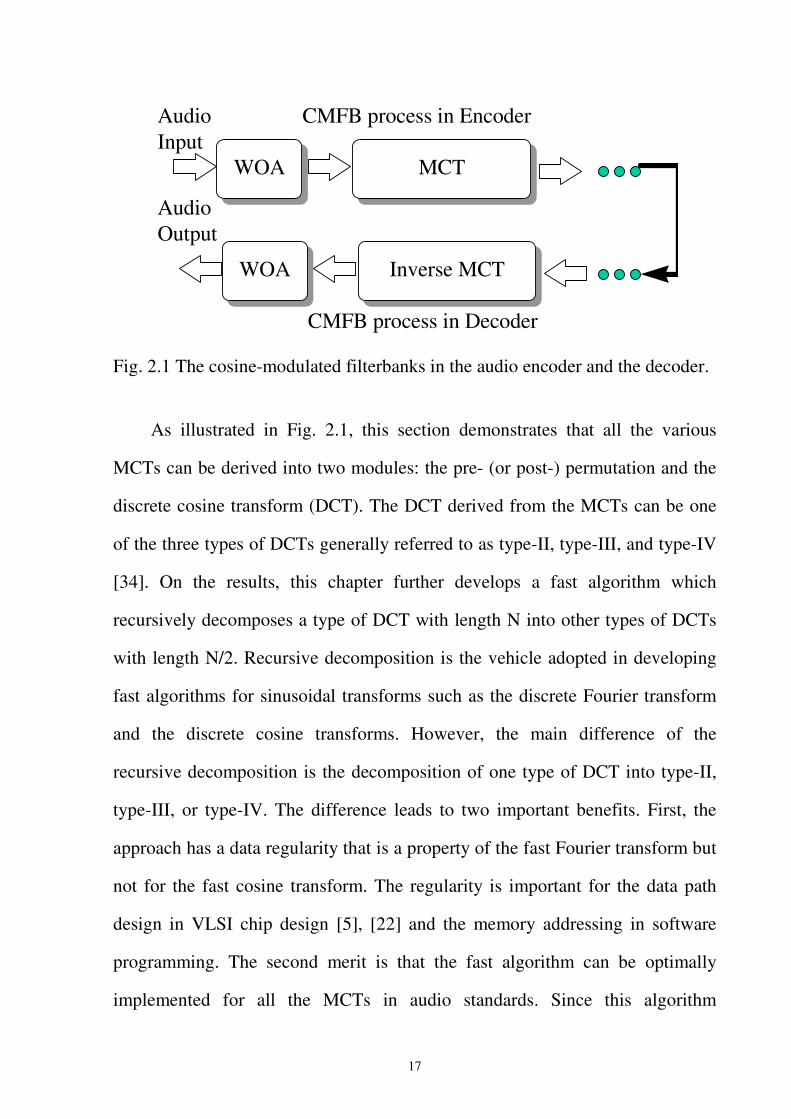
with various audio coding standards. This section demonstrates that all the

20

CMFBs can be represented as the pre- or post-permutation and the discrete

cosine transform (DCT) as shown in Fig. 2.2. The DCT type can be one of the

following three types:

Type-II DCT

1-N ..., 0,1,=kfor 1

0)))(12(

2cos(�

−

=+=

N

iki

NixkXπ .

(2.1)

Type-III DCT

1-N ..., 1, 0,=kfor ))12)((2

cos(1

0� +=

−

=

N

iki

NixkXπ .

(2.2)

Type-IV DCT

1-N ..., 1, 0,=kfor ))12)(12(4

cos(1

0� ++=

−

=

N

iki

NixkXπ .

(2.3)

In equations (2.1)-(2.3), there have been constant terms in front of each formula.

For example the type-IV DCT is

110for ))12)(12(4

cos(2 1

0, ..., N-, k=ki

NixNkX

N

i� ++=

−

=

π .

The constant term N2 is neglected for ease of description.

21

PrepermutationPrepermutation DCTDCT

Inverse DCTInverse DCT

MDCT in the Encoder

MDCT in the Decoder

Output of the WOA

Input of the WOA

PostpermutationPostpermutation

Fig. 2.2 The representation of the MDCT into permutation and the DCT.

2.2.1 Unified form for the MCT in TDAC filterbank

This section illustrates the method to transform the modulated cosine

transform (MCT) in time-domain aliasing cancellation (TDAC) filterbank into

the permutation and the type-IV DCT. The forward and inverse MCT of the

TDAC filterbank are respectively defined as

))12)(2

12(2

cos(1

0� +++=

−

=

N

ik

Ni

NixkXπ for k =0, 1, …, N/2-1.

(2.4)

and

� +++=−

=

12/

0))12)(

212(

2cos(~ N

kk

Ni

NkXixπ for i = 0, 1, …, N-1.

(2.5)

where a constant term before each summation is again neglected for

representation ease. Also note that, unlike the general transform, the sequence

ix~ , in (2.5) is in general not equal to sequence ix in (2.4) given the same kX .

In the following we proceed with the derivation through three steps. First, we

22

extend the transform pair in (2.4) and (2.5) to a form which has length N along

both indices i and k through Theorem 1 and Theorem 2. Second, the extended

transform with length N is represented as a length N transform which is quite

similar to the type-IV DCT as illustrated in Theorem 3 and Theorem 4. Finally,

the DCT-like transform with length N is reduced to type-IV DCT with length

(N/2) with input or output permutation through Theorem 5 and Theorem 6.

Define the following transform pair:

110for ,))12)(2

12(2

cos(1

0, ..., N-, k=k

Ni

NixkXN

i� +++′=′

−

=

π

(2.6)

and

.110for ,))12)(2

12(2

cos(21~ 1

0, ..., N-, i=k

Ni

NkXixN

k� +++′=′

−

=

π

(2.7)

The following two theorems illustrate the relation between the extended

transform and the TDAC transform.

Theorem 1: The sequence kX ′ in (2.6) is anti-symmetric in the sense that

kNk XX −−′−=′ 1 if N is a multiple of 4.

<proof>: Representing kNX −−′ 1 as

10for ))1)1(2)(2

12(2

cos(1

01 ...N- k=kN

Ni

NixXN

ikN � +−−++=′

−

=−−

π

which can be reformulated as

10for ))2

12()21)(2

12(2

cos(1

01 ...N-k=

Nik

Ni

NixXN

ikN � +++−−++=′

−

=−− ππ

Since the transform length N is a multiple of four,

23

))21)(2

12(2

cos(

))21)(2

12(2

cos(

1

0

1

01

kXkN

iNix

kN

iNixX

N

i

N

ikN

′−=� −−++−=

� −−++−=′

−

=

−

=−−

π

π

Theorem 2: Let N be an integer with the multiple of four. Assume that the

sequence kX ′ with length N is obtained by extending the sequence kX with

length (N/2) according to kNk XX −−′−=′ 1 for k=N/2, …, N-1. Given (2.5) and

(2.7) the sequence ix~ computed from (2.5) is equivalent to the sequence ix ′~

computed from (2.7).

<Proof>: From (2.7),

ixkN

iNkXix

N

k′� +++′=′

−

=

~))12)(2

12(2

cos(21~ 1

0

π

Separating the summation into two parts yields

��

��

�

��

��

�� � +++′++++′=′

−

=

−

=

12

0

1

2

))12)(2

12(2

cos())12)(2

12(2

cos(21~

N

k

N

Nk

kN

iNkXk

Ni

NkXixππ

Replacing the index k in the second summation as N-1-k yields

��

��

�

��

��

�

+−−++′++++′=′ � �−

=

−

=−−

12

0

12

01 ))1)1(2)(

212(

2cos())12)(

212(

2cos(

21~

N

k

N

kkNki kN

Ni

NXk

Ni

NXx

ππ

Since kNk XX −−′−=′ 1 and N is a multiple of four, the formula can be further

rewritten as

24

�

� �

−

=

−

=

−

=

=+++′=

��

��

�

��

��

�

+−−++′−+++′=′

12

0

12

0

12

0

~))12)(2

12(2

cos(

))1)1(2)(2

12(2

cos())12)(2

12(2

cos(21~

N

kik

N

k

N

kkki

xkN

iN

X

kNN

iN

XkN

iN

Xx

π

ππ

Through Theorem 1 and Theorem 2, we can compute the MCT transform in

(2.4) and (2.5) through (2.6) and (2.7), respectively. Define the DCT-like

transform as follows

110for ,))12)(12(2

cos(1

0

, ..., N-, k=kiN

uXN

iik �

−

=

++= π

(2.8)

and

110for )),12)(12(2

cos(~1

0

, ..., N-, i=kiN

XuN

kki �

−

=

++= π

(2.9)

The following theorem sets the fundamental to compute TDAC transform

through (2.8) and (2.9).

Theorem 3: Given (2.6) and (2.8), the sequence kX ′ computed through (2.6) is

equivalent to the sequence kX computed through (2.8) if N is a multiple of 4

and the sequence iu in (2.8) is permuted from the sequence ix′ in (2.6)

through the following form

1144

=ifor , ,14

10for ,=u44

3i , ..., N-+N

, N

xuN

, ..., , i=x Ni

iNi −+

=−−

(2.10)

25

<Proof>: Substituting j=i+N/4 into (6) gives

110for ))12)(12(2

cos(14/5

4/

...,N-, k=kjN

xXN

Njik �

−

=

++′=′ π

Representing the summation into two terms yields

1-10for ))12)(12(2

cos(+))12)(12(2

cos(14/51

4/

, ...,N, k=kjN

xkjN

xXN

Njj

N

Njik ��

−

=

−

=

++′++′=′ ππ

(2.11)

Let m=j-N. Since

))12)(12(2

cos())12)(1)(2(2

cos( ++−=+++ kmN

kNmN

ππ ,

(2.11) can be reformulated as

k

N

ii

N

mi

N

Njik

XkjN

u

kmN

xkjN

xX

=++=

++′−++′=′

�

��−

=

−

=

−

=

1

0

14/

0

1

4/

))12)(12(2

cos(

))12)(12(2

cos(+))12)(12(2

cos(

π

ππ

Theorem 4: Given (2.7) and (2.9) with kk XX =′ , the sequence ix ′~ computed

from (2.7) can be obtained from the sequence iu~ computed from (2.9) through

the following permutation:

114

34

3for ,~

21~

14

310for ,~

21

=~

14

7

4

, ..., N-+N

, N

i=ux

N..,, i=ux

iNi

Ni

i

−−

+

=′

−′

(2.12)

<Proof>: From (2.7)

�−

=

+++′=′1

0

))12)(2

12(2

cos(21~

N

kki k

Ni

NXx

π for i=0, 1, ..., N-1.

Consider the summation from two separate parts. For 4

30

Ni <≤ ,

26

��−

=+

−

=

=+++′=+++′=′1

0 4

1

0

~21

))12)(1)4

(2(2

cos(21

))12)(2

12(2

cos(21~

N

kN

ik

N

kki uk

Ni

NXk

Ni

NXx

ππ

For NiN <≤4

3

))12)(1)4

(2(2

cos(21

=x~1

0i �

−

=

+++′′N

kk k

Ni

NX

π

Since )12)(1)12(2(2

cos()12)(12(2

cos( ++−−=++ kiNN

kiN

ππ

�

�−

= −−

−

=

=++−−′

+++−−′′

1

0 14

7

1

0i

~21

))12)(1)14

7(2(

2cos(

21

=

))12)(1))4

(12(2(2

cos(21

=x~

N

k iNk

N

kk

ukiN

NX

kN

iNN

X

π

π

To further derive the relation with type-IV DCT, we consider the following

Lemma:

Lemma 1: The sequence Xk computed through (2.8) is anti-symmetric in the

sense that XN-1-k= -Xk., for k=0, 1, …, N-1.

<Proof> From (2.8),

k

N

ii

N

ii

N

ii

N

ii

N

ii

N

iikN

X

kiN

ukiN

u

kiN

u

iN

NkiN

u

kNiN

u

kNiN

uX

−=

++−=−−+−=

+−−+=

++−−+=

−−+=

+−−+=

��

�

�

�

�

−

=

−

=

−

=

−

=

−

=

−

=−−

1

0

1

0

1

0

1

0

1

0

1

01

))12)(12(2

cos())12)(12(2

cos((

))12)(12(2

cos((

))12(2

2)12)(12(2

cos(

))122)(12(2

cos(

1-N ..., 0,1,=kfor ))1)1(2)(12(2

cos(

ππ

ππ

ππ

π

π

Substituting Lemma 1 into (2.8) yields

27

���

��

�

�++

++=

�

�−

=

−

=

12

for X-

12

10for ))12)(12(2

cos(=

10for ))12)(12(2

cos(

k-1-N

1

0

1

0

...N-N

k=

-N

, ...,, k=kiN

u

...N-k=kiN

uX

N

ii

N

iik

π

π

(2.13)

Representing type-IV DCT with length (N/2) according to (2.3) gives

12

10for ))12)(12(2

cos(

12

0

-N

, ..., , k=kiN

sY

N

iik �

−

=

++= π

(2.14)

The following two theorems set the basis to compute (2.8) and (2.9) through

type-IV DCT in (2.14).

Theorem 5: Given (2.8) and (2.14), the sequence Xk in (2.8) for k=0,

1, …,(N/2)-1 will be equivalent to the sequence Yk in (2.13) if

iNii uus −−−= 1 , for i = 0, 1, ..., (N/2)-1

(2.15)

<Proof> Representing the first term in (2.13) into two summation terms yields

��

��

�

−

= +

−

=

−

= +

−

=

−

=

++−−++=

+++++=

++=

12/

0 2

12/

0

12/

0 2

12/

0

1

0

))12)(1)12

(2(2

cos(- ))12)(12(2

cos(

))12)(1)2

(2(2

cos(+ ))12)(12(2

cos(

1-N/2 ..., 1, 0,=kfor ))12)(12(2

cos(

N

jN

j

N

ii

N

jN

j

N

ii

N

iik

kjN

Nuki

Nu

kN

jN

ukiN

u

kiN

uX

ππ

ππ

π

Let N-1-m=j+(N/2)

28

k

N

iiNi

N

mmN

N

ii

N

mmN

N

iik

YkiN

uu

kmN

ukiN

u

kmNN

Nuki

NuX

=++−=

++++=

++−−−−++=

�

��

��

−

=−−

−

=−−

−

=

−

=−−

−

=

12/

01

12/

01

12/

0

12/

01

12/

0

))12)(12(2

cos()(

))12)(12(2

cos(- ))12)(12(2

cos(

))12)(1))12

(12

(2(2

cos(- ))12)(12(2

cos(

π

ππ

ππ

To proceed with the following derivation, (2.14) is rewritten by interchanging

the indices i and k as follows

12

10for ))12)(12(2

cos(1

2

0

-N

, ..., , i=ikN

sY

N

kki �

−

=

++= π

(2.16)

Theorem 6: Given (2.9) and (2.16) with kk Xs 2= and kX has the

anti-symmetric property described in Lemma 1, the sequence ~iu in (2.9) for

i=0, 1, …,(N/2)-1 is equivalent to the sequence Yi of type-IV DCT in (2.16).

<Proof> From (2.9) 110for )),12)(12(2

cos(~1

0

, ..., N-, i=kiN

XuN

kki �

−

=

++= π

From Lemma 1, XN-1-k= -Xk. Hence

�

�−

=

−

=−−

++=

++−=

12/

0

12/

01

))12)(12(2

cos(2

))12)(12(2

cos()(~

N

kk

N

kkNki

kiN

X

kiN

XXu

π

π

To summarize, the forward MCT in (2.4) can be computed through the

type-IV DCT in (2.14) with the input permutation through (2.10) and (2.15) in

Theorem 3 and Theorem 5. From Theorem 2, Theorem 4, and Theorem 6,

the inverse MCT in (2.5) can be computed through the type-IV DCT in (2.16)

29

with the output permutation in (2.12).

2.2.2 Unified form for the variant of TDAC filterbanks

Two variants of time-domain aliasing cancellation (TDAC) filterbank have

been adopted in the Dolby AC-3 coder to provide the perfect reconstruction

property between different block sizes [43]. The first transform pair is defined as

�−

=

++′=′1

0

))12)(12(2

cos(N

iik ki

NxX

�

�

π , for k=0,1, …, N/2-1

(2.17)

�−

=

++′=′1

2

0

))12)(12(2

cos(~

N

kki ki

NXx

�

�

π , for i=0,1, …, N-1

(2.18)

The second transform pair is

�−

=

+++′′=′′1

0

))12)(12(2

cos(N

iik kNi

NxX

�

�π , for k=0,1, …, N/2-1

(2.19)

�−

=

+++′′=′′1

2

0

))12)(12(2

cos(~N

kki kNi

NXx

�

π , for i=0,1, …, N-1

(2.20)

This section demonstrates that (2.17)-(2.20) can be derived as permutation and

type-IV DCT. First we set the relation between the transform pair in (2.17)-(2.18)

and that in (2.8)-(2.9).

Theorem 7: Let the sequence Xk in (2.9) with length N be obtained by

extending the sequence 1kX with length (N/2) according to Xk = -XN-k-1 for

30

k=N/2, …, N-1. Given (2.9) and (2.18), the sequence iu~ computed from (2.9) is

two times the sequence 1~ix computed from (2.18).

<Proof>: From (2.9),

��

��

�

��

��

�

+++++=

++=

� �

�

−

=

−

=

−

=

12

0

1

2

1

0

))12)(12(2

cos())12)(12(2

cos(

))12)(12(2

cos(~

N

k

N

Nk

kk

N

kki

kiN

XkiN

X

kiN

Xu

ππ

π

Since kNk XX −−−= 1 ,

i

N

kk

N

k

N

kkk

N

k

N

kkNki

xkN

iN

X

kNiN

XkiN

X

kNiN

XkiN

Xu

′=+++=

+−−+−++=

+−−++++=

�

� �

� �

−

=

−

=

−

=

−

=

−

=−−

~2))12)(2

12(2

cos(2

))1)1(2)(12(2

cos())12)(12(2

cos(

))1)1(2)(12(2

cos())12)(12(2

cos(~

12

0

12

0

12

0

12

0

12

01

π

ππ

ππ

Lemma 1 and Theorem 7 set the fundamental to derive the TDAC-variant in

(2.17) and (2.18) through DCT-like transform in (2.8) and (2.9). From Theorem

5 and Theorem 6, the DCT-like transform can be computed through the type-IV

DCT. Hence, the first form of the TDAC-variant transform can be derived into

the permutation and type-IV DCT.

The following two theorems illustrate the relation between the MCT of the

TDAC-variant in (2.17)-(2.18) and that in (2.19)-(2.20).

Theorem 8: Given (2.17) and (2.19), the sequence 2kX in (2.19) is equivalent

to 1kX if

31

1122

;12

10for x22

i −+=′−=′′−′−=′′ −+ ...,��

, �

i xx, N

...,, i=x NN iii

(2.21)

<Proof>: Substituting j=i-N/2 into (2.19) yields

��

�−

=−

−

=−

−

=−

++′′+++′′=

++′′=′′

12/31

2/

12/3

2/

))12)(12(2

cos())12)(12(2

cos(

110for ))12)(12(2

cos(

22

2

N

Njj

N

Njj

N

Njjk

kjN

xkjN

x

, ..., N-, k=kjN

xX

NN

N

��

��

��

ππ

π

Let m=j-N

��−

=+

−

=− +++′′+++′′=′′

12/

0

1

2/

))12)(122(2

cos())12)(12(2

cos(22

N

mm

N

Njjk kNm

Nxkj

NxX NN

��

��

ππ

Since

))12)(12(2

cos())12)(122(2

cos( ++−=+++ kmN

kNmN ��

ππ

k

N

mm

N

Njjk

X

kmN

xkjN

xX NN

′=

++′′−++′′=′′ ��−

=+

−

=−

12/

0

1

2/

))12)(12(2

cos())12)(12(2

cos(22 �

��

�ππ

Theorem 9: Given (2.18) and (2.20), the sequence 2~ix in (2.20) is equivalent to

1~ix if

1122

~~12

10for ~x~22

i −+′=′′−′−=′′ −+ ...,NN

, N

i=xx, N

...,, i=x NN iii

(2.22)

<Proof>: From (2.20),

�−

=

+++′′=′′12

0

))12)(1)2

(2(2

cos(~N

kki k

Ni

NXx

�

π , for i=0,1, …, N-1

For N/2<i0 ≤

2

~))12)(1)2

(2(2

cos(~12

0

Ni

N

kki xk

Ni

NXx +

−

=

′=+++′′=′′ � �

π

32

For N<iN/2 ≤

2

~))12)(1)2

(2(2

cos(

))12)(1)2

(2(2

cos(~

12/

0

12/

0

Ni

N

kk

N

kki

xkNN

iN

X

kN

iN

Xx

−

−

=

−

=

′−=++−+′′−=

+++′′=′′

�

�

�

�

π

π

The computation of the two variants of TDAC filterbank defined in equations

(2.17)-(2.20) can be computed with the following remarks:

Computing Process for (2.17): From Theorem 5, the MCT of the first

TDAC-variant in (2.17) can be computed directly through the type-IV DCT in

(2.14) with the input permutation

iNii xxs −−′−′= 1 , for i = 0, 1, ..., (N/2)-1

(2.23)

Computing Process for (2.18): From Theorem 6 and Theorem 7, the inverse

MCT of the first TDAC-variant in (2.18) can be computed directly through the

type-IV DCT in (2.16).

Computing Process for (2.19): From Theorem 5 and Theorem 8, the MCT of

the second TDAC-variant in (2.19) can be computed directly through the

type-IV DCT in (2.14) with the input permutation in (2.21) and (2.23).

Computing Process for (2.20): From Theorem 6, Theorem 7 and Theorem 9 the

inverse MCT of the second TDAC-variant in (2.20) can be computed directly

through the type-IV DCT in (2.16) through the output permutation in (2.22).

2.2.3 Unified form for the polyphase filterbank

The transform pair for the cosine modulation transform in the polyphase

33

filterbank [43] is

12

10 ))12)(4

(cos(1

0

-N

, ..., , k=kN

iN

xXN

iik �

−

=

+−= π

(2.24)

110 ))12)(4

(cos(~12/

0

..., N-, i=kN

iN

XxN

kki �

−

=

++= π

(2.25)

To proceed with the derivation, we define the following two transform formulae

12

10for ))12)((cos(1

0

-N

..., , k= kiN

uXN

iik �

−

=

+=′ π

(2.26)

110for ))12)((cos(~12/

0

..., N-, i=kiN

XuN

kki �

−

=

+′= π

(2.27)

The derivation proceeds with two steps. First, we show (2.24) and (2.25) can be

computed through (2.26) and (2.27) with permutation through Theorem 10 and

Theorem 11. Second, we show (2.26) and (2.27) can be computed through

type-III DCT through Theorem 12 and Theorem 13.

Theorem 10: Let N be an integer that is a multiple of four. Given (2.24) and

(2.26), the sequence kX ′ computed through (2.26) is equivalent to the sequence

kX computed through (2.24) if

114

34

3 1

43

10 4

34

−+−==−+

, ..., NN

, N

i=xu-N

, ..., , i=xu Ni

iNi

i

(2.28)

<Proof>: Let j=i-N/4. Rewrite (2.24) as

34

1)2/(...,,1,0,))12)((cos())12)((cos(14/3

0 4

1

44

−=+++= ��−

=+

−

−=+

NkforkjN

xkjN

xXN

jN

jNj

Nj

kππ

Let m=j+N. Since

))12)((cos())12)((cos( +−=+− kmN

kNmN

ππ

k

N

jN

j

N

mN

mk Xkj

Nxkm

NxX

N

′=+++−= ��−

=+

−

=−

14/3

0 4

1

43 ))12)((cos())12)((cos(

43

ππ

Theorem 11: Let N is a multiple of four. Given (2.25) and (2.27) and kk XX ′= ,

the sequence ix~ computed through (2.25) can be permuted from the sequence iu~

computed through (2.27) with the following form

1,,14

34

3for ~~ and 1

43

,1,0for ~~4/3i4/ N-...+

N,

Ni=ux-

N ... i=ux NiNii −+ −==

(2.29)

<Proof >: Rewrite (2.25) as

110 ))12)(4

(cos(~12/

0

...,N-, i=kN

iN

XxN

kki �

−

=

++= π

For 3N/4<i0 ≤

4N

+i

12/

0

u~= ))12)(4

(cos(~ �−

=

++=N

kki k

Ni

NXx

π

For N<i3N/4 ≤

4/3

12/

0

12/

0

~))12)(4

(cos(-= ))12)(4

(cos(~Ni

N

kk

N

kki ukN

Ni

NXk

Ni

NXx −

−

=

−

=

−=+−+++= ��ππ

According to(2.1), type-II DCT with length (N/2) is

12

10for )))(12(cos(

12

0

-N

, ..., ,i=ikN

xX

N

kki �

−

=

+= π

35

(2.30)

Theorem 12: Given (2.27) and (2.30), let kk xX =′ . The sequence iu~ computed

through (2.27) can be obtained from sequence iX through

���

�

���

�

�

− 1-22

12

for ~

12

10for =~

2for 0=~

...., N+N

, +N

i==-Xu

-N

, ..., , i=Xu

i=N/u

iNi

ii

i

(2.31)

<Proof>: Rewrite (2.27) as

110for ))12)((cos(~12/

0

..., N-, i=kiN

XuN

kki �

−

=

+′= π

For 2

0N

i<≤

i

N

kki Xki

NXu = ))12)((cos(~

12/

0�

−

=+′= π

For 2N

i= ,

0= ))12(2

cos(~12/

0�

−

=+′=

N

kki kXu

π

For i<NN ≤+12

, since

12

1012

21for ) )12)((cos())12)((cos( -N

..., , , k=-N

..., , i=kiNN

kiN

+−−=+ ππ ,

we have the following relation

��−

=−

−

=−=+−′−=+′=

12/

0

12/

0

))12)((cos())12)((cos(~N

kiNk

N

kki XkiN

NXki

NXu

ππ

According to (2.2), type-III DCT with length (N/2) is

36

12

10for ))12)((cos(

12

0

-N

, ..., , k=kiN

xX

N

iik �

−

=

+= π

(2.32)

Theorem 13: Given (2.26) and (2.32), the sequence kX in (2.32) is equivalent

to the sequence kX ′ in (2.26) if the sequence ix is computed from the sequence

iu through

12

1 for1

00

��

��

�

−=

=

−− -N

, ..., i=uux

ux

iNii

(2.33)

<Proof>: From (2.26)

�

�

�

−

=−

−

=

−

=

+−++

++++=

+=′

12/

12

12/

10

1

0

))12)((cos())12)(4

(cos(

))12)((cos())12)(0(cos(

1-N/21..., 0,=kfor , ))12)((cos(

N

iiNN

N

ii

N

iik

kiNN

ukN

Nu

kiN

ukN

u

kiN

uX

ππ

ππ

π

Since

0))12)(4

(cos( 2

=+kN

NuN

π

and

))12)((cos())12)((4

cos( +−=+− kiN

kiNN

ππ

k

N

iiNik Xki

Nuuk

NuX =+−++=′ �

−

=−−

1

110 ))12)((cos()())12)(0(cos()(

ππ

The MCT in (2.24) can be computed through the type-III DCT in (2.32) with the

input permutation through (2.28) and (2.33) in Theorem 10 and Theorem 13.

37

From Theorem 10 and Theorem 12, the inverse MCT in (2.25) can be

computed through the type-II DCT in (2.30) with the output permutation in

(2.29) and (2.31).

2.3 Fast Algorithm for the Discrete Cosine Transform

Section 2.2 illustrates that the various cosine-modulated transforms used in

TDAC, TDAC-variant, and polyphase filterbanks can be divided into two

modules: permutation and the DCT. Especially, the forward transform can be

represented as the pre-permutation and the DCT while the inverse transform as

the DCT and the post-permutation. The DCT can be type-II, type-III, or type-IV.

This section develops a method to decompose a type of DCT with length N into

two of the three types of the DCT with length N/2. The decomposition method

will be proved to have the regularity and the modularity in additional to the low

complexity. Furthermore, the algorithm is applicable to the cosine-modulated

transforms in audio coding standards.

2.3.1 Decomposition for type-II DCT

From (2.1), the kth coefficient of the type-II DCT for an input sequence xi with

length N is

1-0for )))(12(2

cos(1

0

...Nk=kiN

xXN

iik �

−

=

+= π

We first decompose Xk of the type-II DCT into even-indexed and odd-indexed

forms. The even-indexed output sequence is

38

12

0for , ))2)(12(2

cos(1

02 -

N, ...,k=ki

NxX

N

iik �

−

=

+= π .

(2.34)

Applying the symmetry property ))(12(cos())(1)1(2(cos( kiN

kiNN

+=+−− ππ gives

�−

=−− ++

12/

012 )))(12(cos()(=

N

iiNik ki

NxxX

π

(2.35)

which is a type-II DCT with input permutation.

The odd-indexed output sequence is

12

0for , ))12)(12(2

cos(1

012 -

N, ..., i=ki

NxX

N

iik �

−

=+ ++= π

Applying the anti-symmetry property

)12)(1)1(2(2

cos()12)(12(2

cos( ++−−−=++ kiNN

kiN

ππ

gives

))12)(12(2

cos()(1-N/2

0=i112 � ++−= −−+ ki

NxxX iNik

π

(2.36)

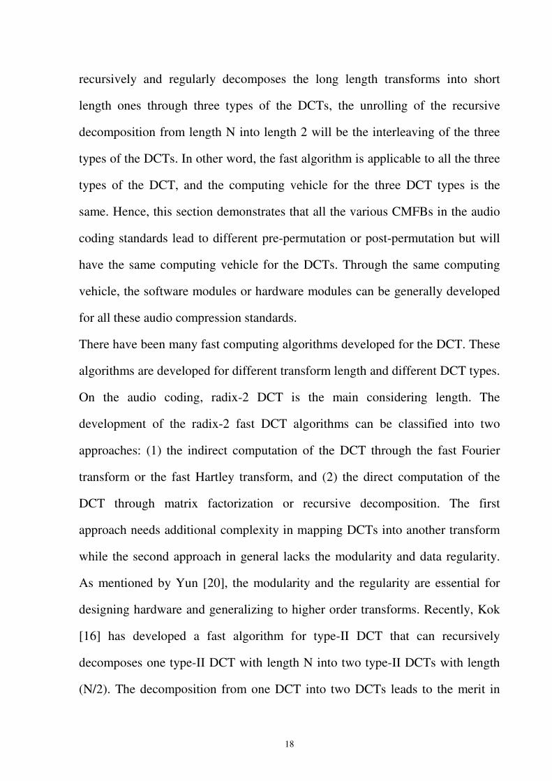
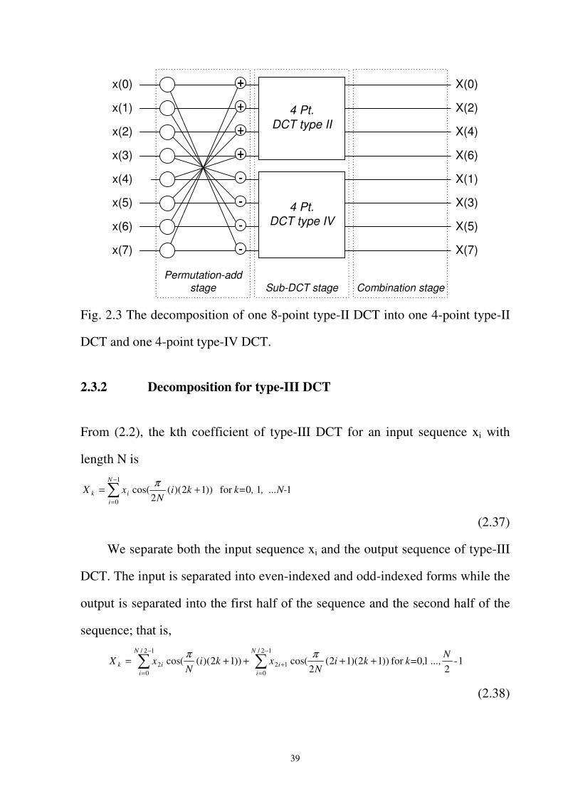
which is a type-IV DCT with input permutation. From (2.35) and (2.36), a

type-II DCT with length N can be decomposed into one type-II DCT and one

type-IV with length (N/2) as illustrated in Fig. 2.3.

39

Combination stagePermutation-add

stage Sub-DCT stage

x(0)

x(1)

x(2)

x(3)

x(5)

x(6)

x(7)

4 Pt.DCT type II

4 Pt.DCT type IV

X(0)

X(2)

X(4)

X(6)

X(1)

X(3)

X(5)

X(7)

x(4)

Fig. 2.3 The decomposition of one 8-point type-II DCT into one 4-point type-II

DCT and one 4-point type-IV DCT.

2.3.2 Decomposition for type-III DCT

From (2.2), the kth coefficient of type-III DCT for an input sequence xi with

length N is

110for ))12)((2

cos(1

0

, ...N-, k=kiN

xXN

iik �

−

=

+= π

(2.37)

We separate both the input sequence xi and the output sequence of type-III

DCT. The input is separated into even-indexed and odd-indexed forms while the

output is separated into the first half of the sequence and the second half of the

sequence; that is,

1-2

10for ))12)(12(2

(cos))12)(((cos12/

012

12/

02

N ...,,k=ki

Nxki

NxX

N

ii

N

iik ++++= ��

−

=+

−

=

ππ

(2.38)

40

1-2

10for )),1)2

(2)(12(2

(cos))1)2

(2)(((cos12/

012

12/

02

2

N, ...,,k=

Nki

Nx

Nki

NxX

N

ii

N

ii

kN ++++++= ��

−

=+

−

=+

ππ

(2.39)

Substituting

))1)12

(2)((cos())1)2

(2)((cos( +−−=++ kN

iN

Nki

Nππ

and

))1)12

(2)(12(cos())1)2

(2)(12(cos( +−−+−=+++ kN

iN

Nki

Nππ

into (2.39) yields

120for

))1)12

(2)(12(2

(cos))1)12

(2)(((cos12/

012

12/

02

2

-...N/k=

kN

iN

xkN

iN

xXN

ii

N

ii

kN +−−+−+−−= ��

−

=+

−

=+

ππ.

(2.40)

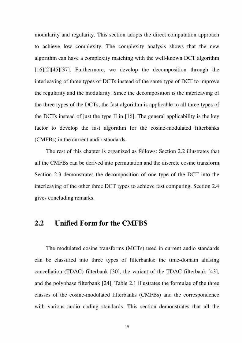
From (2.38) and (2.40), a type-III DCT with length N can be decomposed into

one type-III DCT and one type-IV DCT with length (N/2) as illustrated in Fig.

2.4.

Combination stagePermutation-add

stage Sub-DCT stage

x(1)

x(3)

x(5)

x(7)

x(2)

x(4)

x(6)

4 Pt.DCT type IV

4 Pt.DCT type III

X(0)

X(1)

X(2)

X(3)

X(4)

X(5)

X(6)

X(7)x(0)

41

Fig. 2.4 The decomposition of one 8-point type-III DCT into one 4-point

type-III DCT and one 4-point type-IV DCT.

2.3.3 Decomposition for type-IV DCT

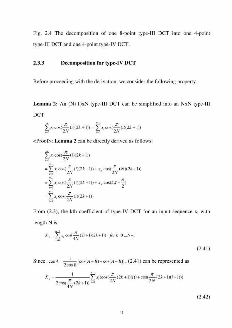
Before proceeding with the derivation, we consider the following property.

Lemma 2: An (N+1)xN type-III DCT can be simplified into an NxN type-III

DCT

))12)((2

(cos))12)((2

(cos1

00

+=+ ��−

==

kiN

xkiN

xN

ii

N

ii

ππ

<Proof>: Lemma 2 can be directly derived as follows:

))12)((2

(cos

)2

cos())12)((2

(cos=

))12)((2

cos())12)((2

(cos=

))12)((2

(cos

1

0

1

0

1

0

0

+=

+++

+++

+

�

�

�

�

−

=

−

=

−

=

=

kiN

x

kxkiN

x

kNN

xkiN

x

kiN

x

N

ii

N

N

ii

N

N

ii

N

ii

π

πππ

ππ

π

From (2.3), the kth coefficient of type-IV DCT for an input sequence xi with

length N is

1-0 ))12)(12(4

cos(1

0

...Nfor k=kiN

xXN

iik �

−

=

++= π

(2.41)

Since ))cos()(cos(cos2

1cos BABA

BA −++= , (2.41) can be represented as

)))1)(12(2

cos()))(12(2

((cos))12(

4cos(2

1=

1

0

+++++

�−

=ik

Nik

Nx

kN

XN

iik

πππ

(2.42)

42

Separating input sequences into even and odd terms yields

})22)(12(2

cos()12)(12(2

cos(

)12)(12((cos)2)(12((cos{))12(

4cos(2

1

12/

012

12/

02

12/

012

12/

02

��

��

−

=+

−

=

−

=+

−

=

++++++

+++++

=

N

ii

N

ii

N

ii

N

iik

ikN

xikN

x

ikN

xikN

xk

N

X

ππ

πππ

(2.43)

Set 01 == N- x x , the four terms in (2.43) can be represented as

}))12)(12(2

cos()())(12((cos)({

))12(4

cos(2

1

12/

0122

2/

0122 ��

−

=+

=− ++++++

+=

N

iii

N

iii

k

ikN

xxikN

xx

kN

X

ππ

π

From Lemma 2,

}))12)(12(2

cos()()))(12((cos)({

))12(4

cos(2

1

12/

0122

12/

0122 ��

−

=+

−

=− ++++++

+=

N

iii

N

iii

k

ikN

xxikN

xx

kN

X

ππ

π

(2.44)

From (2.44), a type-IV DCT with length N can be decomposed into one type-IV

DCT and one type-III DCT with length (N/2) as illustrated in Fig. 2.5.

43

Combination stagePermutation-add stage Sub-DCT stage

x(0)

x(2)

x(4)

x(6)

x(1)

x(3)

x(5)

x(7)

4 Pt.DCT type IV

4 Pt.DCT type III

X(0)

X(1)

X(2)

X(3)

X(7)

X(6)

X(5)

X(4)

x

x

x

x

x

x

x

x

x(8)=x(-1)=0

Fig. 2.5 The decomposition of one 8-point type-IV DCT into one 4-point

type-III DCT and one 4-point type-IV DCT.

From Fig. 2.3-Fig. 2.5, the arithmetic complexities for all three types of the DCT

are individually

DCT-II(N)= A(N)+DCT-IV(N/2)+DCT-II(N/2),

DCT-III(N)=A(N)+DCT-IV(N/2)+DCT-III(N/2),

and DCT-IV(N)=A(N-1)+M(N)+DCT-IV(N/2)+DCT-III(N/2)

where DCT-II(N), DCT-III(N), and DCT-IV(N) are the arithmetic complexity of

the type-II, type-III, and type-IV DCT with length N. A(µ) and M(κ) indicate

the number of real addition and multiply are µ and κ, respectively. Table 2.2

lists the arithmetic complexity of the new algorithm and the existing

algorithms[2][16][37][45] for the radix-2 DCTs. The results illustrate that the

fast algorithm not only unifies the computing methods for types II, III, and IV

DCT but also has a complexity as low as the well-known algorithms.

44

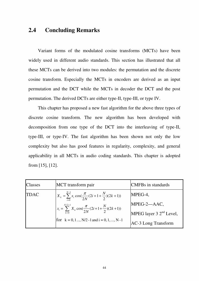
2.4 Concluding Remarks

Variant forms of the modulated cosine transforms (MCTs) have been

widely used in different audio standards. This section has illustrated that all

these MCTs can be derived into two modules: the permutation and the discrete

cosine transform. Especially the MCTs in encoders are derived as an input

permutation and the DCT while the MCTs in decoder the DCT and the post

permutation. The derived DCTs are either type-II, type-III, or type IV.

This chapter has proposed a new fast algorithm for the above three types of

discrete cosine transform. The new algorithm has been developed with

decomposition from one type of the DCT into the interleaving of type-II,

type-III, or type-IV. The fast algorithm has been shown not only the low

complexity but also has good features in regularity, complexity, and general

applicability in all MCTs in audio coding standards. This chapter is adopted

from [15], [12].

Classes MCT transform pair CMFBs in standards

TDAC ))12)(2

12(2

cos(1

0�

−

=

+++=N

iik k

Ni

NxX

π

))12)(2

12(2

cos(12/

0�

−

=

+++=N

kki k

Ni

NXx

π

for 1-N ..., 1, 0,=i and 1-N/2 ..., 1 0,=k

MPEG-4,

MPEG-2—AAC,

MPEG layer 3 2nd Level,

AC-3 Long Transform

45

�−

=

++=1

0

))12)(12(2

cos(N

iik ki

NxX

�

�

π

�−

=

++=12/

0

))12)(12(2

cos(N

kki ki

NXx

�

�

π

for 1-N ..., 1, 0,=i and 1-N/2 ..., 1 0,=k

AC-3 Short Transform 1 TDAC-Variant

�−

=

+++=1

0

))12)(12(2

cos(N

iik kNi

NxX

�

��

�π

�−

=

+++=12/

0

))12)(12(2

cos(N

kki kNi

NXx

�

��

π

for 1-N ..., 1, 0,=i and 1-N/2 ..., 1 0,=k

AC-3 Short Transform 2

Polyphase

Filter Bank

))12)(4

(cos(1

0�

−

=

+−=N

iik k

Ni

NxX

π

))12)(4

(2

cos(12/

0�

−

=

++=N

iki k

Ni

NXx

π

for 1-N ..., 1, 0,=i and 1-N/2 ..., 1 0,=k

MPEG layers 1, 2,

MPEG layer 3 1st Level

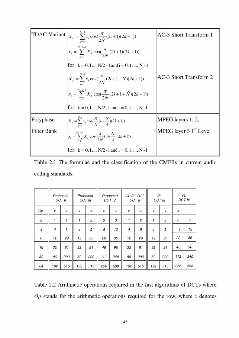
Table 2.1 The formulae and the classification of the CMFBs in current audio

coding standards.

8

Op.

16

32

64

2

4

12 29 20 36

x + x +

[4],[9], [10]DCT II

[4]DCT IV

32 81 48 96

80 209 112 240

192 513 256 588

1 2 3 3

4 9 8 12

20 36

x +

ProposedDCT IV

48 96

112 240

256 588

3 3

8 12

12 29

x +

ProposedDCT III

32 81

80 209

192 513

1 2

4 9

12 29

x +

ProposedDCT II

32 81

80 209

192 513

1 2

4 9

12 29

x +

[8]DCT III

32 81

80 209

192 513

1 2

4 9

Table 2.2 Arithmetic operations required in the fast algorithms of DCTs where

Op stands for the arithmetic operations required for the row, where x denotes

46

multiplication operation while + addition operation. The 2, 4, 8, 16, 32, and 64

in first column denote the transform length. The entries of the row associating

with the transform length illustrate the operations required for the algorithm

labeled in the entry of the first row of the column.

47

Chapter 3 Fast Frequency Analysis for the Psychoacoustic Model

3.1 Introduction

For the perceptual audio coder as illustrated in Fig. 1.1, the frequency

analyzer are required in the psychoacoustic model and the filterbank. In the

psychoacoustic model, frequency information is required to model hearing

model and thus a frequency analysis is required. For filterbank, frequency

analysis is necessary to transform signals from time domain to frequency

domain to remove the redundancy from the psychoacoustic model. A summary

on frequency analysis schemes in filterbanks and psychoacoustic model are

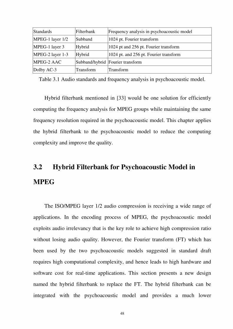
given in Table 3.1. For MPEG group, the frequency analysis on filterbank and

psychoacoustic model is implemented in different approaches: Fourier transform

and subband/hybrid filterbank. AC-3 coder uses the same frequency analyzer in

both filterbank and psychoacoustic model. Obviously, from the viewpoint of the

computation loading, the design of AC-3 coder is more efficient than the one of

MPEG group due to the redundant computation of frequency analysis on

psychoacoustic model and filterbank.

48

Standards Filterbank Frequency analysis in psychoacoustic model

MPEG-1 layer 1/2 Subband 1024 pt. Fourier transform

MPEG-1 layer 3 Hybrid 1024 pt and 256 pt. Fourier transform

MPEG-2 layer 1-3 Hybrid 1024 pt. and 256 pt. Fourier transform

MPEG-2 AAC Subband/hybrid Fourier transform

Dolby AC-3 Transform Transform

Table 3.1 Audio standards and frequency analysis in psychoacoustic model.

Hybrid filterbank mentioned in [33] would be one solution for efficiently

computing the frequency analysis for MPEG groups while maintaining the same

frequency resolution required in the psychoacoustic model. This chapter applies

the hybrid filterbank to the psychoacoustic model to reduce the computing

complexity and improve the quality.

3.2 Hybrid Filterbank for Psychoacoustic Model in

MPEG

The ISO/MPEG layer 1/2 audio compression is receiving a wide range of

applications. In the encoding process of MPEG, the psychoacoustic model

exploits audio irrelevancy that is the key role to achieve high compression ratio

without losing audio quality. However, the Fourier transform (FT) which has

been used by the two psychoacoustic models suggested in standard draft

requires high computational complexity, and hence leads to high hardware and

software cost for real-time applications. This section presents a new design

named the hybrid filterbank to replace the FT. The hybrid filterbank can be

integrated with the psychoacoustic model and provides a much lower

49

complexity than the FT. Also, this section shows that the hybrid filter is more

suitable for the stereo coding and hence can provide a better quality for the

intensity stereo coding, which is the key technology for the MPEG-1 to achieve

near transparent quality lower than 96x2 kbits for two stereo channels.

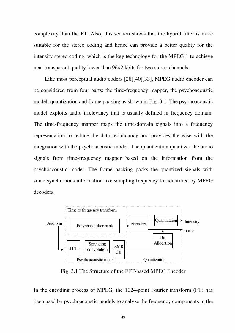
Like most perceptual audio coders [28][40][33], MPEG audio encoder can

be considered from four parts: the time-frequency mapper, the psychoacoustic

model, quantization and frame packing as shown in Fig. 3.1. The psychoacoustic

model exploits audio irrelevancy that is usually defined in frequency domain.

The time-frequency mapper maps the time-domain signals into a frequency

representation to reduce the data redundancy and provides the ease with the

integration with the psychoacoustic model. The quantization quantizes the audio

signals from time-frequency mapper based on the information from the

psychoacoustic model. The frame packing packs the quantized signals with

some synchronous information like sampling frequency for identified by MPEG

decoders.

FFTSpreading

convolutionSMRCal.

Psychoacoustic model

Polyphase filter bank

BitAllocation

Audio in Normalize Intensity

phase

Quantization

Quantization

Time to frequency transform

Fig. 3.1 The Structure of the FFT-based MPEG Encoder

In the encoding process of MPEG, the 1024-point Fourier transform (FT) has

been used by psychoacoustic models to analyze the frequency components in the

50

1152 samples of one frame. If the conventional real-data fast FT (FFT)

[19] has been adopted for implementing the FT, the complexity has an order of

(4*256*log(512)). Such a complexity leads to high implementation cost for

real-time applications.

This section presents a new design named the hybrid filterbank to replace

the FT. The hybrid filterbank can be integrated with the psychoacoustic models

and provides a much lower complexity than the FT. Also, this section shows that

the hybrid filter is more suitable for the stereo coding and hence can provide a

better quality for the intensity stereo coding, which is the key technology for the

MPEG-1 to achieve near transparent quality lower than 96x2 kbits for two stereo

channels.

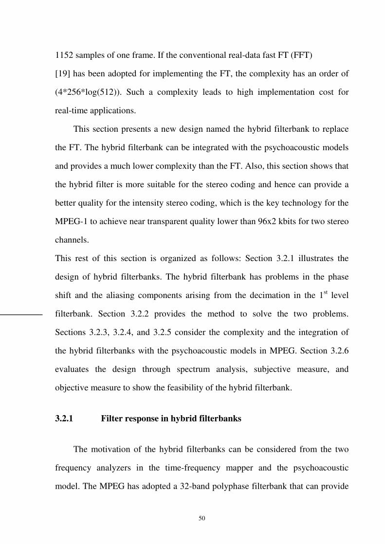
This rest of this section is organized as follows: Section 3.2.1 illustrates the

design of hybrid filterbanks. The hybrid filterbank has problems in the phase

shift and the aliasing components arising from the decimation in the 1st level

filterbank. Section 3.2.2 provides the method to solve the two problems.

Sections 3.2.3, 3.2.4, and 3.2.5 consider the complexity and the integration of

the hybrid filterbanks with the psychoacoustic models in MPEG. Section 3.2.6

evaluates the design through spectrum analysis, subjective measure, and

objective measure to show the feasibility of the hybrid filterbank.

3.2.1 Filter response in hybrid filterbanks

The motivation of the hybrid filterbanks can be considered from the two

frequency analyzers in the time-frequency mapper and the psychoacoustic

model. The MPEG has adopted a 32-band polyphase filterbank that can provide

51

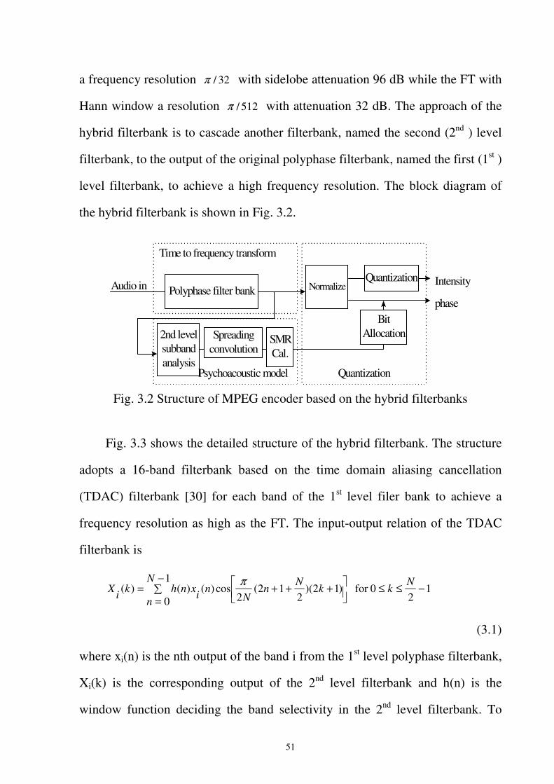
a frequency resolution 32/π with sidelobe attenuation 96 dB while the FT with

Hann window a resolution 512/π with attenuation 32 dB. The approach of the

hybrid filterbank is to cascade another filterbank, named the second (2nd ) level

filterbank, to the output of the original polyphase filterbank, named the first (1st )

level filterbank, to achieve a high frequency resolution. The block diagram of

the hybrid filterbank is shown in Fig. 3.2.

2nd levelsubbandanalysis

Spreadingconvolution

SMRCal.

Psychoacoustic model

Polyphase filter bank

BitAllocation

Audio in Normalize Intensity

phase

Quantization

Quantization

Time to frequency transform

Fig. 3.2 Structure of MPEG encoder based on the hybrid filterbanks

Fig. 3.3 shows the detailed structure of the hybrid filterbank. The structure

adopts a 16-band filterbank based on the time domain aliasing cancellation

(TDAC) filterbank [30] for each band of the 1st level filer bank to achieve a

frequency resolution as high as the FT. The input-output relation of the TDAC

filterbank is

12

0for 1

0)12)(

212(

2cos)()()( −≤≤�

−

=

��

� +++= Nk

N

nk

Nn

NnixnhkiX

π

(3.1)

where xi(n) is the nth output of the band i from the 1st level polyphase filterbank,

Xi(k) is the corresponding output of the 2nd level filterbank and h(n) is the

window function deciding the band selectivity in the 2nd level filterbank. To

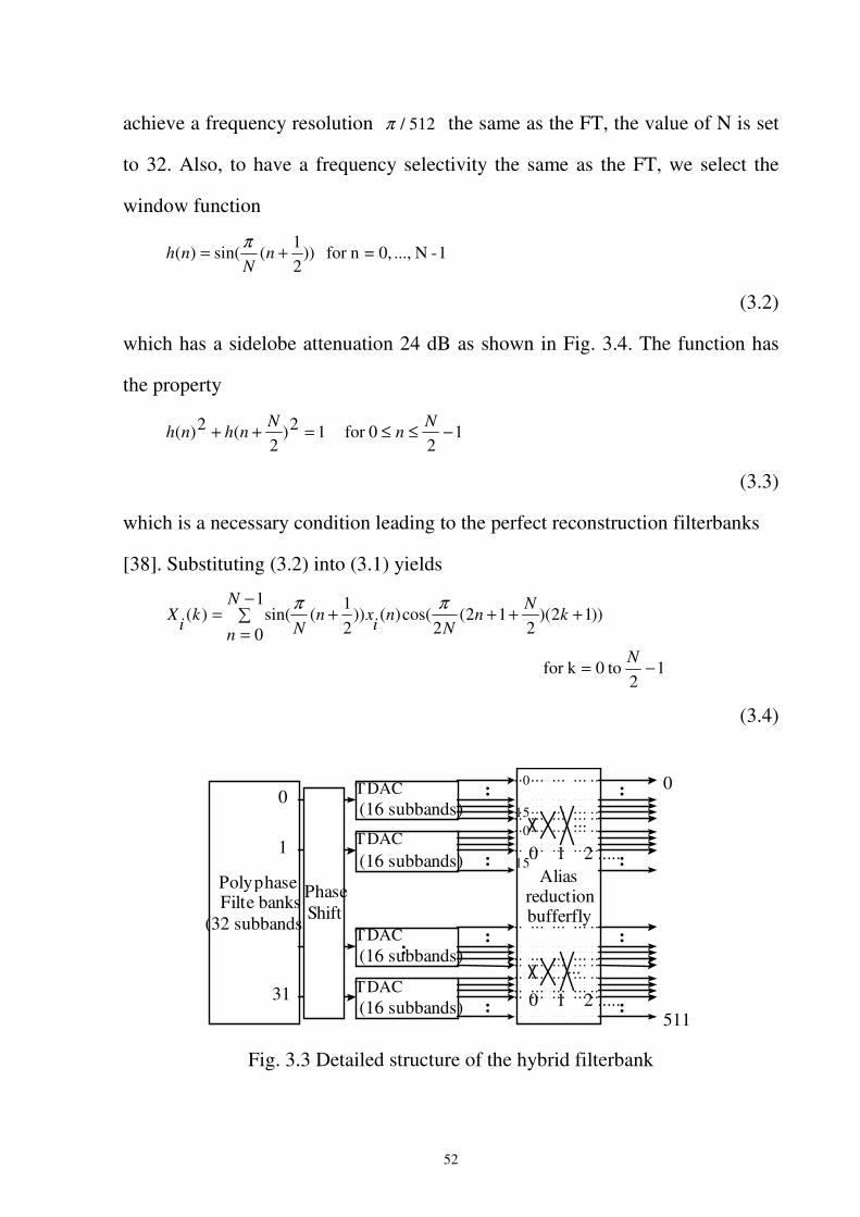
52

achieve a frequency resolution π / 512 the same as the FT, the value of N is set

to 32. Also, to have a frequency selectivity the same as the FT, we select the

window function

1-N ..., 0,=nfor ))21

(sin()( += nN

nhπ

(3.2)

which has a sidelobe attenuation 24 dB as shown in Fig. 3.4. The function has

the property

12

0for 12)2

(2)( −≤≤=++ Nn

Nnhnh

(3.3)

which is a necessary condition leading to the perfect reconstruction filterbanks

[38]. Substituting (3.2) into (3.1) yields

12

to0kfor

1

0 ))12)(

212(

2cos()())

21

(sin()(

−=

�−

=++++=

N

N

nk

Nn

Nnixn

NkiX

ππ

(3.4)

Polyphase Filte banks

(32 subbands)

TDAC (16 subbands)

TDAC (16 subbands)

TDAC (16 subbands)

TDAC (16 subbands)

:

Alias reduction bufferfly

:

:

:

:

:

:

:

0

15 0

15

0

1

31

0

511

Phase Shift

:

...

...

0 1 2 .....

0 1 2 .....

Fig. 3.3 Detailed structure of the hybrid filterbank

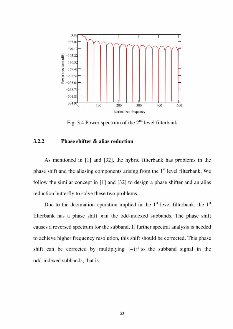
53

0 100 200 300 400 500334.91

301.81

268.71

235.61

202.51

169.41

136.32

103.22

70.12

37.02

3.92

Normalized frequency

Pow

er s

pect

urm

(dB

)

Fig. 3.4 Power spectrum of the 2nd level filterbank

3.2.2 Phase shifter & alias reduction

As mentioned in [1] and [32], the hybrid filterbank has problems in the

phase shift and the aliasing components arising from the 1st level filterbank. We

follow the similar concept in [1] and [32] to design a phase shifter and an alias

reduction butterfly to solve these two problems.

Due to the decimation operation implied in the 1st level filterbank, the 1st

filterbank has a phase shift π in the odd-indexed subbands. The phase shift

causes a reversed spectrum for the subband. If further spectral analysis is needed

to achieve higher frequency resolution, this shift should be corrected. This phase

shift can be corrected by multiplying − to the subband signal in the

odd-indexed subbands; that is

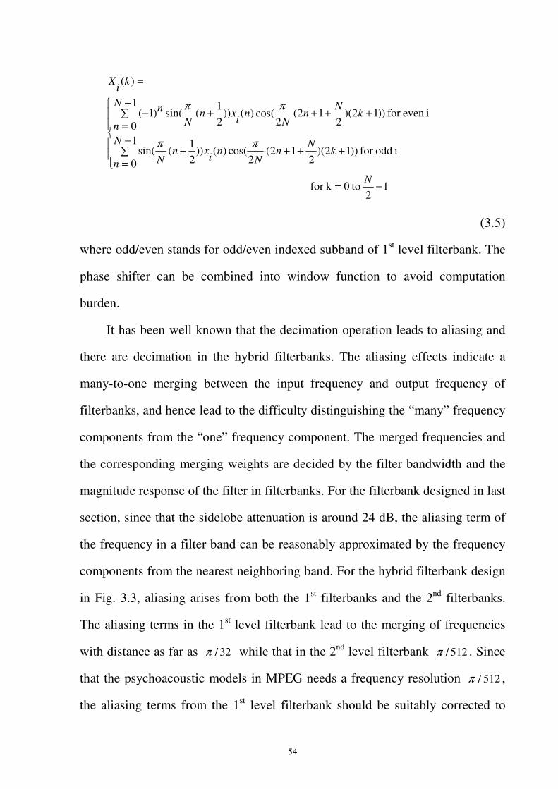
54

12

to0kfor

1

0i oddfor ))12)(

212(

2cos()())

21

(sin(

1

0ieven for ))12)(

212(

2cos()())

21

(sin()1(

)(

−=

��

�

��

�

�

�−

=++++

�−

=++++−

=

N

N

nk

Nn

Nnixn

N

N

nk

Nn

Nnixn

Nn

kiX

ππ

ππ

(3.5)

where odd/even stands for odd/even indexed subband of 1st level filterbank. The

phase shifter can be combined into window function to avoid computation

burden.

It has been well known that the decimation operation leads to aliasing and

there are decimation in the hybrid filterbanks. The aliasing effects indicate a

many-to-one merging between the input frequency and output frequency of

filterbanks, and hence lead to the difficulty distinguishing the “many” frequency

components from the “one” frequency component. The merged frequencies and

the corresponding merging weights are decided by the filter bandwidth and the

magnitude response of the filter in filterbanks. For the filterbank designed in last

section, since that the sidelobe attenuation is around 24 dB, the aliasing term of

the frequency in a filter band can be reasonably approximated by the frequency

components from the nearest neighboring band. For the hybrid filterbank design

in Fig. 3.3, aliasing arises from both the 1st filterbanks and the 2nd filterbanks.

The aliasing terms in the 1st level filterbank lead to the merging of frequencies

with distance as far as 32/π while that in the 2nd level filterbank 512/π . Since

that the psychoacoustic models in MPEG needs a frequency resolution 512/π ,

the aliasing terms from the 1st level filterbank should be suitably corrected to

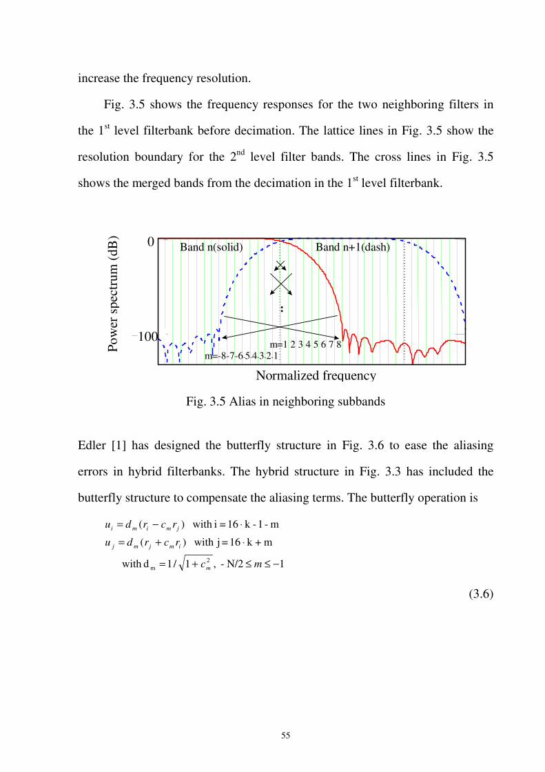
55

increase the frequency resolution.

Fig. 3.5 shows the frequency responses for the two neighboring filters in

the 1st level filterbank before decimation. The lattice lines in Fig. 3.5 show the

resolution boundary for the 2nd level filter bands. The cross lines in Fig. 3.5

shows the merged bands from the decimation in the 1st level filterbank.

100

0

Normalized frequency

Po

wer

spe

ctru

m (d

B)

Band n(solid) Band n+1(dash)

m=1 2 3 4 5 6 7 8 m=-8-7-6-5-4-3-2-1

:

Fig. 3.5 Alias in neighboring subbands

Edler [1] has designed the butterfly structure in Fig. 3.6 to ease the aliasing

errors in hybrid filterbanks. The hybrid structure in Fig. 3.3 has included the

butterfly structure to compensate the aliasing terms. The butterfly operation is

1N/2- ,1/1d with

m+k16=j with)(

m-1-k16=i with)(

2m −≤≤+=

⋅+=

⋅−=

mc

rcrdu

rcrdu

m

imjmj

jmimi

(3.6)

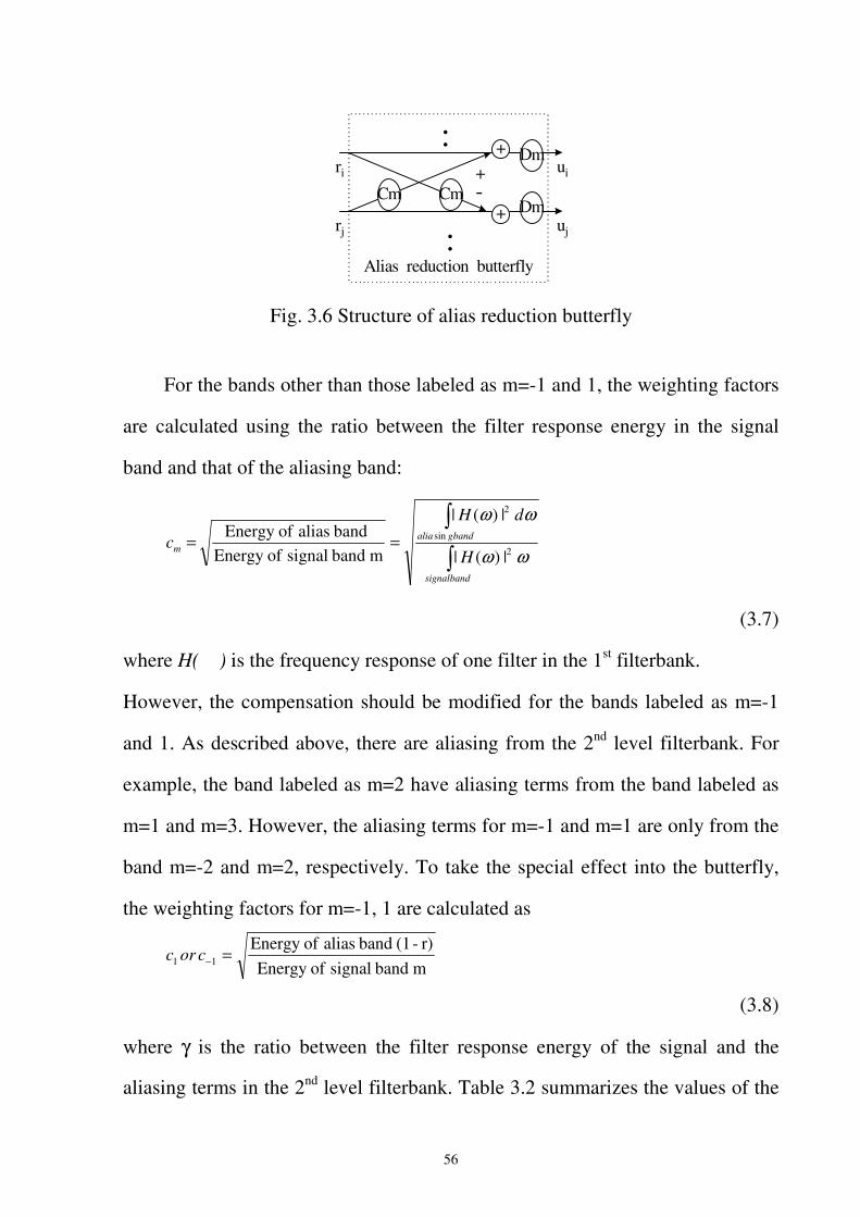
56

Alias reduction butterfly

CmCm

+

+

Dm

Dm

ri

rj

ui

uj

:

:

-+

Fig. 3.6 Structure of alias reduction butterfly

For the bands other than those labeled as m=-1 and 1, the weighting factors

are calculated using the ratio between the filter response energy in the signal

band and that of the aliasing band:

�

�==

bandsignal

bandgaliam

H

dH

cωω

ωω

2

sin

2

|)(|

|)(|

m band signal ofEnergy band alias ofEnergy

(3.7)

where H( ) is the frequency response of one filter in the 1st filterbank.

However, the compensation should be modified for the bands labeled as m=-1

and 1. As described above, there are aliasing from the 2nd level filterbank. For

example, the band labeled as m=2 have aliasing terms from the band labeled as

m=1 and m=3. However, the aliasing terms for m=-1 and m=1 are only from the

band m=-2 and m=2, respectively. To take the special effect into the butterfly,

the weighting factors for m=-1, 1 are calculated as

m band signal ofEnergy r)-(1 band alias ofEnergy

11 =−corc

(3.8)

where γ is the ratio between the filter response energy of the signal and the

aliasing terms in the 2nd level filterbank. Table 3.2 summarizes the values of the

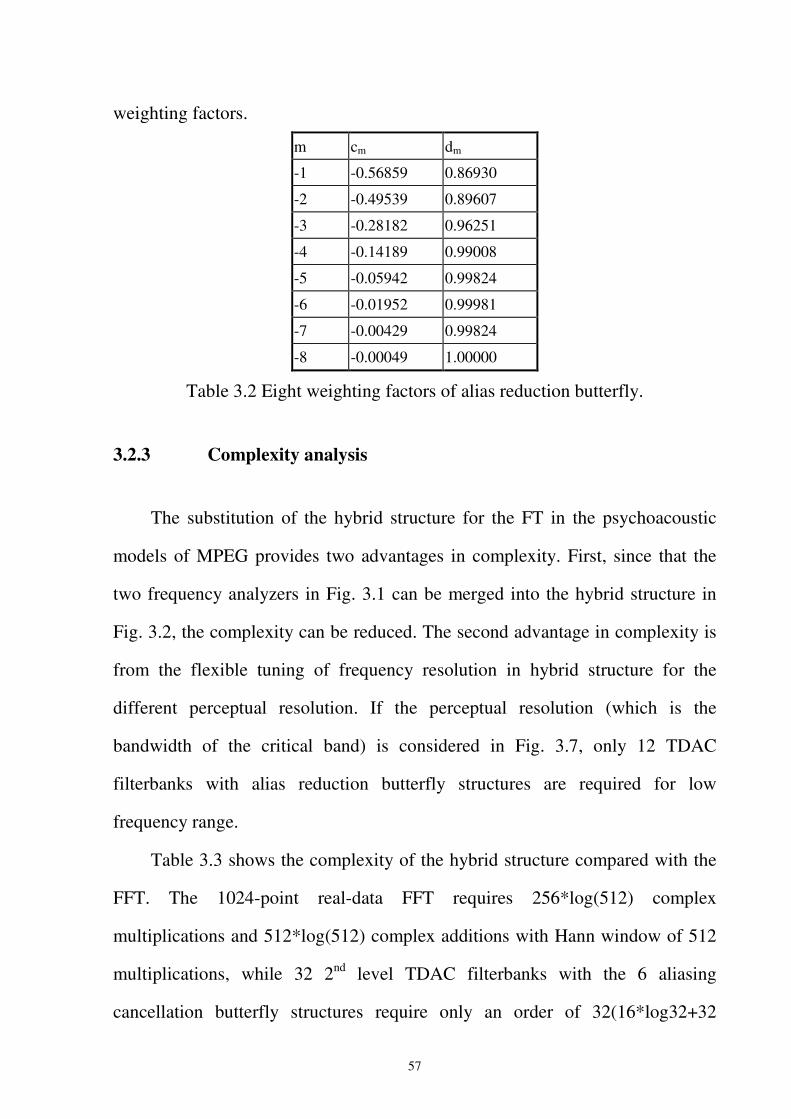
57

weighting factors.

m cm dm

-1 -0.56859 0.86930

-2 -0.49539 0.89607

-3 -0.28182 0.96251

-4 -0.14189 0.99008

-5 -0.05942 0.99824

-6 -0.01952 0.99981

-7 -0.00429 0.99824

-8 -0.00049 1.00000

Table 3.2 Eight weighting factors of alias reduction butterfly.

3.2.3 Complexity analysis

The substitution of the hybrid structure for the FT in the psychoacoustic

models of MPEG provides two advantages in complexity. First, since that the

two frequency analyzers in Fig. 3.1 can be merged into the hybrid structure in

Fig. 3.2, the complexity can be reduced. The second advantage in complexity is

from the flexible tuning of frequency resolution in hybrid structure for the

different perceptual resolution. If the perceptual resolution (which is the

bandwidth of the critical band) is considered in Fig. 3.7, only 12 TDAC

filterbanks with alias reduction butterfly structures are required for low

frequency range.

Table 3.3 shows the complexity of the hybrid structure compared with the

FFT. The 1024-point real-data FFT requires 256*log(512) complex

multiplications and 512*log(512) complex additions with Hann window of 512

multiplications, while 32 2nd level TDAC filterbanks with the 6 aliasing

cancellation butterfly structures require only an order of 32(16*log32+32

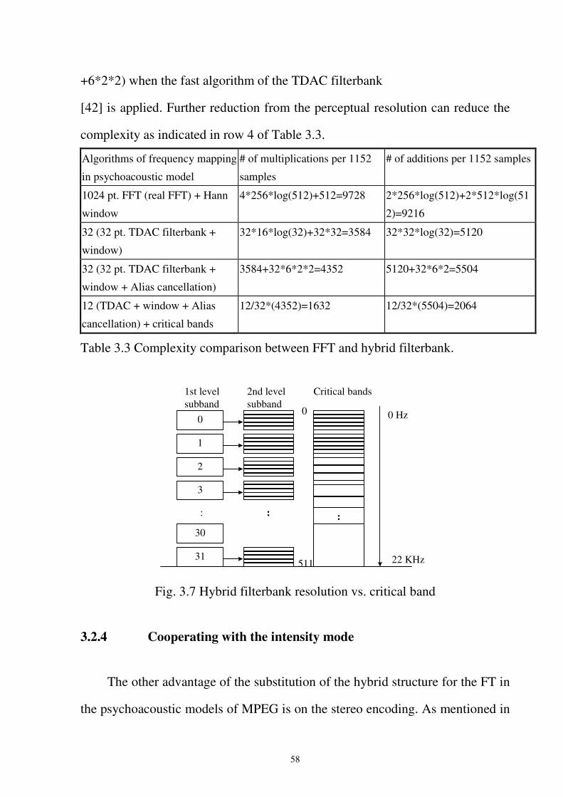
58

+6*2*2) when the fast algorithm of the TDAC filterbank

[42] is applied. Further reduction from the perceptual resolution can reduce the

complexity as indicated in row 4 of Table 3.3.

Algorithms of frequency mapping

in psychoacoustic model

# of multiplications per 1152

samples

# of additions per 1152 samples

1024 pt. FFT (real FFT) + Hann

window

4*256*log(512)+512=9728 2*256*log(512)+2*512*log(51

2)=9216

32 (32 pt. TDAC filterbank +

window)

32*16*log(32)+32*32=3584 32*32*log(32)=5120

32 (32 pt. TDAC filterbank +

window + Alias cancellation)

3584+32*6*2*2=4352 5120+32*6*2=5504

12 (TDAC + window + Alias

cancellation) + critical bands

12/32*(4352)=1632 12/32*(5504)=2064

Table 3.3 Complexity comparison between FFT and hybrid filterbank.

0

1

2

3

30

31

: : :

0 Hz

22 KHz

1st level subband

2nd levelsubband

Critical bands

0

511

Fig. 3.7 Hybrid filterbank resolution vs. critical band

3.2.4 Cooperating with the intensity mode

The other advantage of the substitution of the hybrid structure for the FT in

the psychoacoustic models of MPEG is on the stereo encoding. As mentioned in

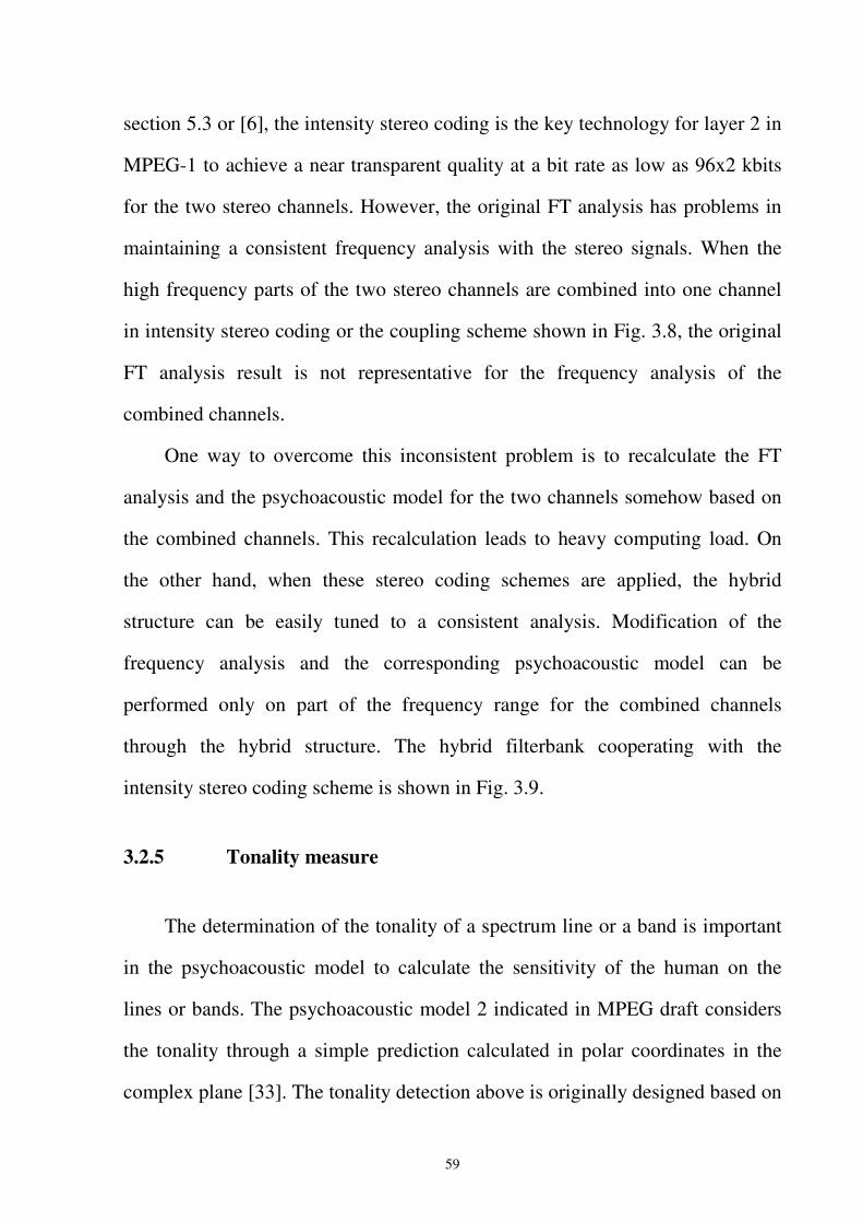
59

section 5.3 or [6], the intensity stereo coding is the key technology for layer 2 in

MPEG-1 to achieve a near transparent quality at a bit rate as low as 96x2 kbits

for the two stereo channels. However, the original FT analysis has problems in

maintaining a consistent frequency analysis with the stereo signals. When the

high frequency parts of the two stereo channels are combined into one channel

in intensity stereo coding or the coupling scheme shown in Fig. 3.8, the original

FT analysis result is not representative for the frequency analysis of the

combined channels.

One way to overcome this inconsistent problem is to recalculate the FT

analysis and the psychoacoustic model for the two channels somehow based on

the combined channels. This recalculation leads to heavy computing load. On

the other hand, when these stereo coding schemes are applied, the hybrid

structure can be easily tuned to a consistent analysis. Modification of the

frequency analysis and the corresponding psychoacoustic model can be

performed only on part of the frequency range for the combined channels

through the hybrid structure. The hybrid filterbank cooperating with the

intensity stereo coding scheme is shown in Fig. 3.9.

3.2.5 Tonality measure

The determination of the tonality of a spectrum line or a band is important

in the psychoacoustic model to calculate the sensitivity of the human on the

lines or bands. The psychoacoustic model 2 indicated in MPEG draft considers

the tonality through a simple prediction calculated in polar coordinates in the

complex plane [33]. The tonality detection above is originally designed based on

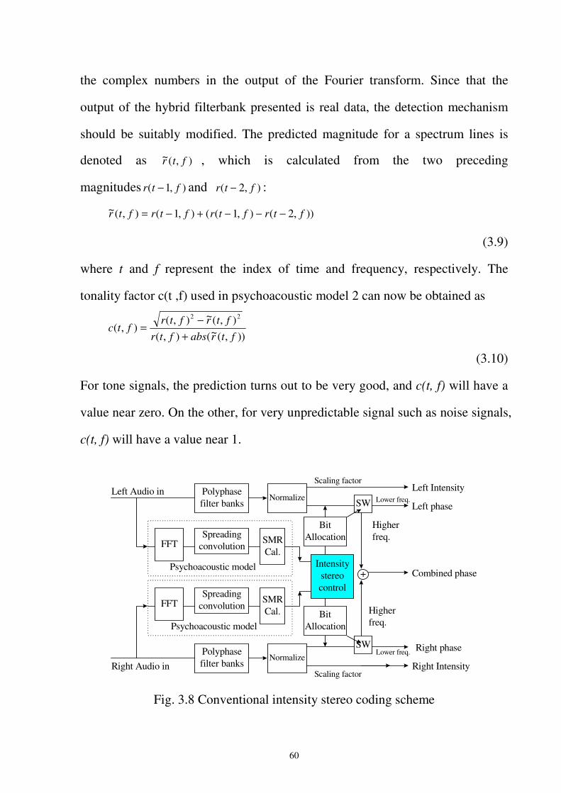
60

the complex numbers in the output of the Fourier transform. Since that the

output of the hybrid filterbank presented is real data, the detection mechanism

should be suitably modified. The predicted magnitude for a spectrum lines is

denoted as ),(~ ftr , which is calculated from the two preceding

magnitudes ),1( ftr − and ),2( ftr − :

)),2(),1((),1(),(~ ftrftrftrftr −−−+−=

(3.9)

where t and f represent the index of time and frequency, respectively. The

tonality factor c(t ,f) used in psychoacoustic model 2 can now be obtained as

)),(~(),(),(~),(

),(22

ftrabsftrftrftr

ftc+

−=

(3.10)

For tone signals, the prediction turns out to be very good, and c(t, f) will have a

value near zero. On the other, for very unpredictable signal such as noise signals,

c(t, f) will have a value near 1.

FFTSpreading

convolutionSMRCal.

Psychoacoustic model

Polyphasefilter banks

BitAllocation

Left Audio in

Polyphasefilter banks

FFTSpreading

convolutionSMRCal.

Psychoacoustic model

Right Audio in

Intensitystereocontrol

Normalize

Scaling factor

Normalize

Scaling factor

BitAllocation

Lower freq.

Higherfreq.

Higherfreq.

Lower freq.

Left Intensity

Right Intensity

Combined phase

Left phase

Right phase

+

SW

SW

Fig. 3.8 Conventional intensity stereo coding scheme

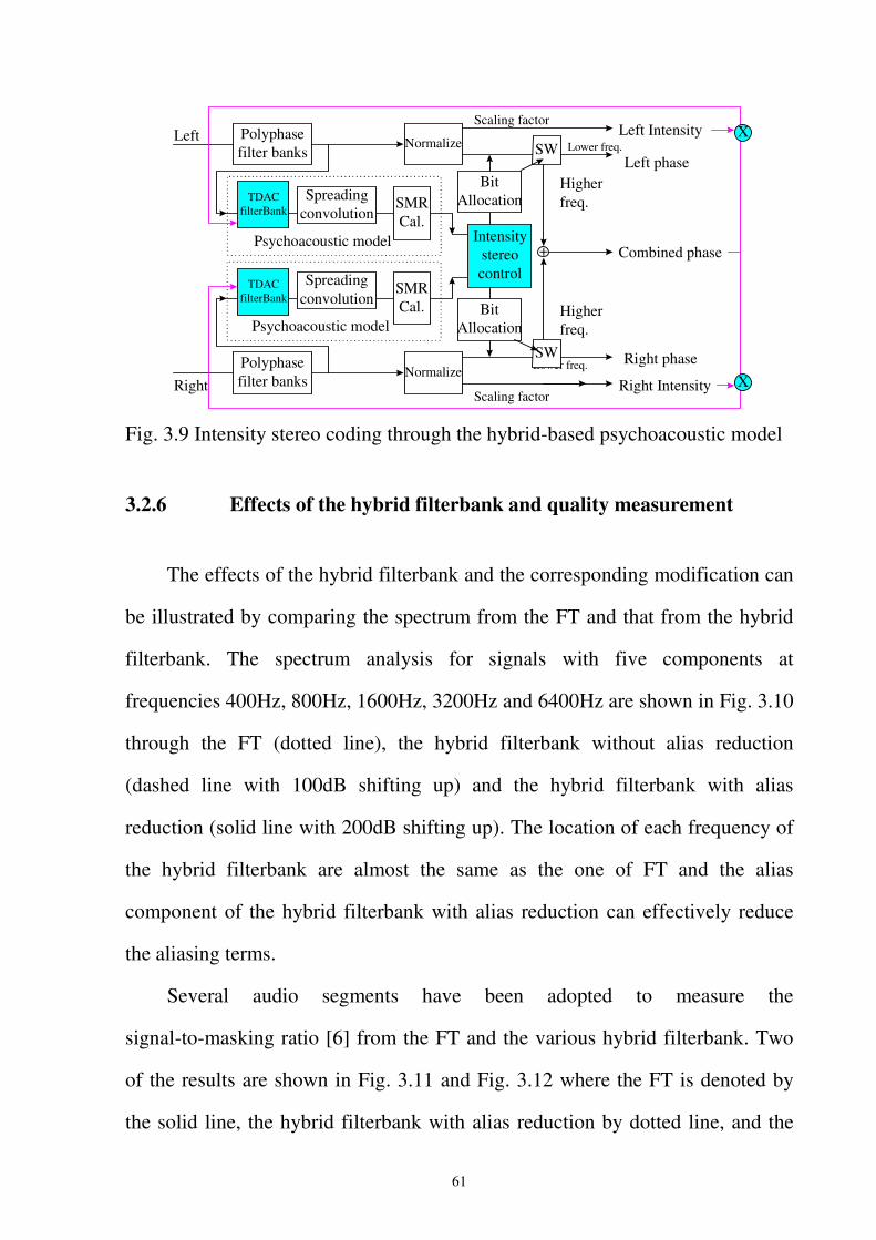
61

TDACfilterBank

Spreadingconvolution

SMRCal.

Psychoacoustic model

Polyphasefilter banks

BitAllocation

Left

Polyphasefilter banks

Spreadingconvolution

SMRCal.

Psychoacoustic model

Right

Intensitystereocontrol

Normalize

Scaling factor

Normalize

Scaling factor

BitAllocation

Lower freq.

Higherfreq.

Higherfreq.

Lower freq.

Left Intensity

Right Intensity

Combined phase

Left phase

Right phase

X

X

+

SW

SW

TDACfilterBank

Fig. 3.9 Intensity stereo coding through the hybrid-based psychoacoustic model

3.2.6 Effects of the hybrid filterbank and quality measurement

The effects of the hybrid filterbank and the corresponding modification can

be illustrated by comparing the spectrum from the FT and that from the hybrid

filterbank. The spectrum analysis for signals with five components at

frequencies 400Hz, 800Hz, 1600Hz, 3200Hz and 6400Hz are shown in Fig. 3.10

through the FT (dotted line), the hybrid filterbank without alias reduction

(dashed line with 100dB shifting up) and the hybrid filterbank with alias

reduction (solid line with 200dB shifting up). The location of each frequency of

the hybrid filterbank are almost the same as the one of FT and the alias

component of the hybrid filterbank with alias reduction can effectively reduce

the aliasing terms.

Several audio segments have been adopted to measure the

signal-to-masking ratio [6] from the FT and the various hybrid filterbank. Two

of the results are shown in Fig. 3.11 and Fig. 3.12 where the FT is denoted by

the solid line, the hybrid filterbank with alias reduction by dotted line, and the

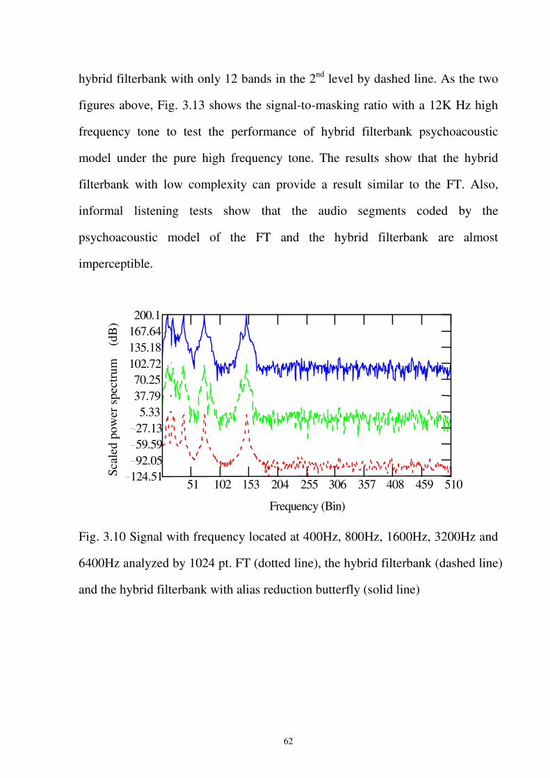
62

hybrid filterbank with only 12 bands in the 2nd level by dashed line. As the two

figures above, Fig. 3.13 shows the signal-to-masking ratio with a 12K Hz high

frequency tone to test the performance of hybrid filterbank psychoacoustic

model under the pure high frequency tone. The results show that the hybrid

filterbank with low complexity can provide a result similar to the FT. Also,

informal listening tests show that the audio segments coded by the

psychoacoustic model of the FT and the hybrid filterbank are almost

imperceptible.

51 102 153 204 255 306 357 408 459 510 124.51 92.05 59.59 27.13 5.33

37.79 70.25

102.72 135.18 167.64 200.1

Frequency (Bin)

Scal

ed p

ower

spe

ctru

m

(dB

)

Fig. 3.10 Signal with frequency located at 400Hz, 800Hz, 1600Hz, 3200Hz and

6400Hz analyzed by 1024 pt. FT (dotted line), the hybrid filterbank (dashed line)

and the hybrid filterbank with alias reduction butterfly (solid line)

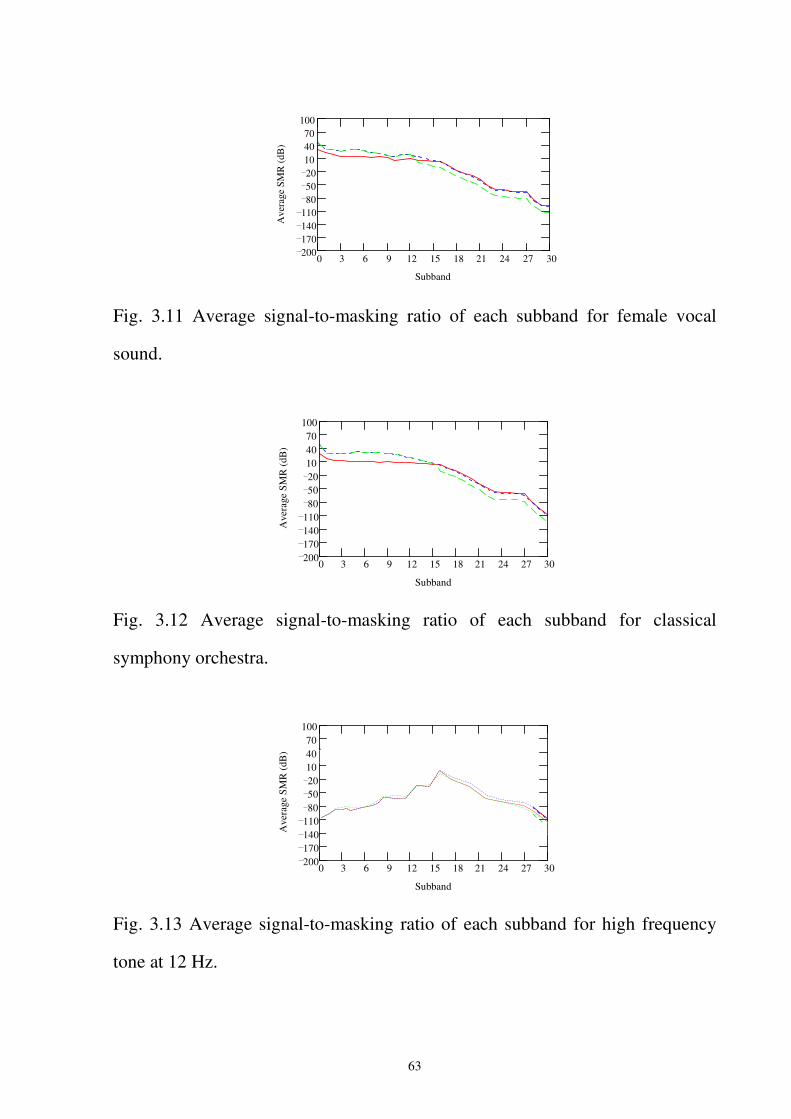
63

0 3 6 9 12 15 18 21 24 27 30200170140110805020104070

100

SubbandA

vera

ge S

MR

(dB

)

Fig. 3.11 Average signal-to-masking ratio of each subband for female vocal

sound.

0 3 6 9 12 15 18 21 24 27 30200170140110805020104070

100

Subband

Ave

rage

SM

R (d

B)

Fig. 3.12 Average signal-to-masking ratio of each subband for classical

symphony orchestra.

0 3 6 9 12 15 18 21 24 27 30200170140110805020104070

100

Subband

Ave

rage

SM

R (d

B)

Fig. 3.13 Average signal-to-masking ratio of each subband for high frequency

tone at 12 Hz.

64

3.3 Concluding Remarks

This section has presented a new design named hybrid filterbanks to

replace the FT adopted in the psychoacoustic model suggested in the draft on the

MPEG layer 1/2 audio coding. This section has given the means to solve the

phase shift and aliasing problems in the hybrid structure. The hybrid filterbank

can be well integrated with the psychoacoustic model and provide a much lower

complexity than the FT. We have also shown that the hybrid filterbank can

cooperate with intensity stereo coding scheme to obtain higher audio quality.

Due to the flexibility of the hybrid filterbank, a consistent psychoacoustic model

with the intensity stereo coding channel can be obtained with little computation

increasing. The hybrid filterbank is tested through spectrum analysis, subjective

measure, and objective measure to show the feasibility.

65

Chapter 4 Fast Bit Allocation Method

Subband and transform coder generate frequency domain decomposition of

audio signals. When considering with the knowledge of human hearing, this

approach offers the possibility to encode the subband components in a way that

minimize the audibility of quantization noise. The quantization noise can be

minimized, when subband components are to quantize in different quantizer

resolution. The quantizer resolution is increase when more bits are assigned to

this transform component. The total bit number for the subband components is

fixed by the design of bit rate of audio coder. A bit allocation algorithm

dynamically distributes the fixed bit pool over the subband component to make

the audible noise minimized.

The bit allocation is aimed to assign suitable parameters to the encoder to

achieve the best audio quality under the restricted bit number. Hence control

over the quality and the bit numbers are two fundamental requirements for the

bit allocation. The complexity of the task depends on the difficulties to have the

quality and bit control. For MPEG Layers 1 and 2, both the quality and the bit

requirement are controlled by a uniform quantizer. Hence the bit allocation is

just to apportion the total number of bits available for the quantization of the

subband signals to minimize the audibility of the quantization noise.

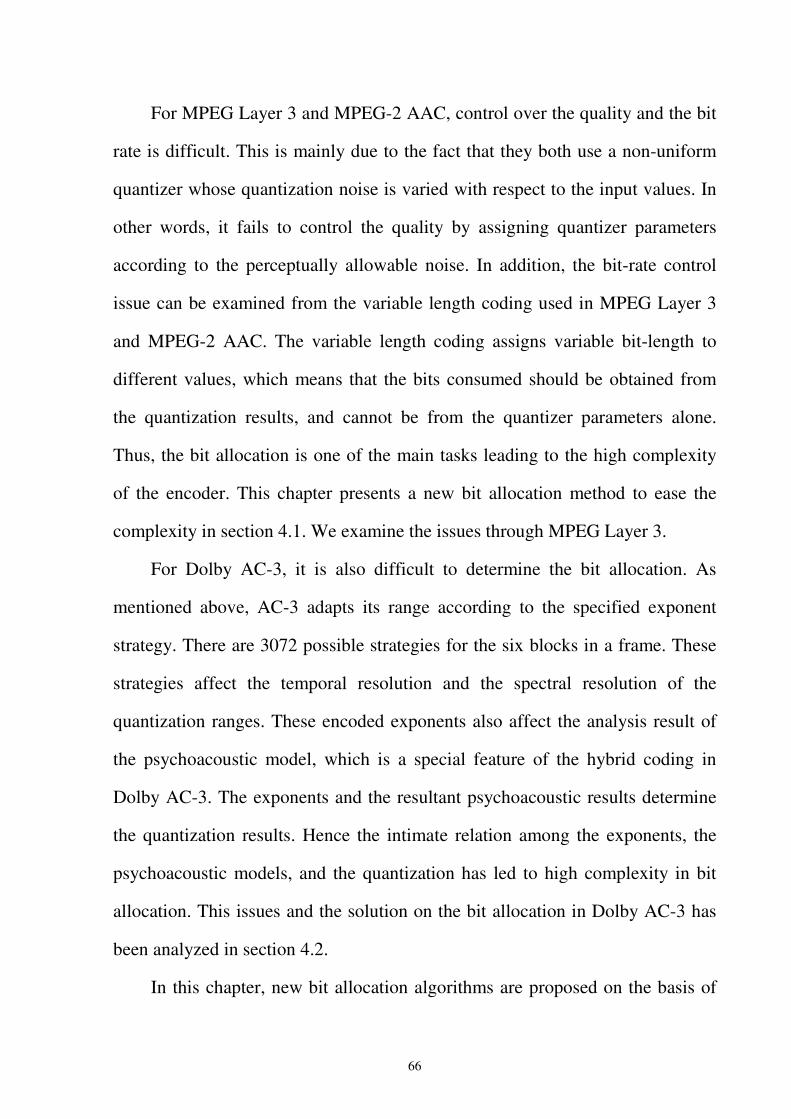
66

For MPEG Layer 3 and MPEG-2 AAC, control over the quality and the bit

rate is difficult. This is mainly due to the fact that they both use a non-uniform

quantizer whose quantization noise is varied with respect to the input values. In

other words, it fails to control the quality by assigning quantizer parameters

according to the perceptually allowable noise. In addition, the bit-rate control

issue can be examined from the variable length coding used in MPEG Layer 3

and MPEG-2 AAC. The variable length coding assigns variable bit-length to

different values, which means that the bits consumed should be obtained from

the quantization results, and cannot be from the quantizer parameters alone.

Thus, the bit allocation is one of the main tasks leading to the high complexity

of the encoder. This chapter presents a new bit allocation method to ease the

complexity in section 4.1. We examine the issues through MPEG Layer 3.

For Dolby AC-3, it is also difficult to determine the bit allocation. As

mentioned above, AC-3 adapts its range according to the specified exponent

strategy. There are 3072 possible strategies for the six blocks in a frame. These

strategies affect the temporal resolution and the spectral resolution of the

quantization ranges. These encoded exponents also affect the analysis result of

the psychoacoustic model, which is a special feature of the hybrid coding in

Dolby AC-3. The exponents and the resultant psychoacoustic results determine

the quantization results. Hence the intimate relation among the exponents, the

psychoacoustic models, and the quantization has led to high complexity in bit

allocation. This issues and the solution on the bit allocation in Dolby AC-3 has

been analyzed in section 4.2.

In this chapter, new bit allocation algorithms are proposed on the basis of

67

MPEG and AC-3 coder standard. The bit allocation algorithms will yield to

close-form bit allocation equations to minimize the audible noise under a fixed

bit rate constraint. The close-form bit allocation equations allow single step bit

allocation. Thus, comparing to the iterative bit allocation design of MPEG and

AC-3, computing complexity is much lower.

4.1 Introduction

From

[44], the perceptual optimal solution for subband bit allocation is the quantized

noise for each subband should be a ratio to masking threshold. That is,

Noise-to-Mask ratio (NMR) in dB will be a constant for each subband. As

shown in Fig. 4.1, the noise energy curve for different bit rate, Noisek#1 and

Noisek#2 are parallel to masking threshold curve Maskingk in dB.

��Signal, masking, noise (Fig.)

Frequency (kHz)

Energy (dB)

Signalk

Maskingk

Noisek #1

Noisek #2

Fig. 4.1 The relation of optimal noise shaping for different bit rate for Noise 1

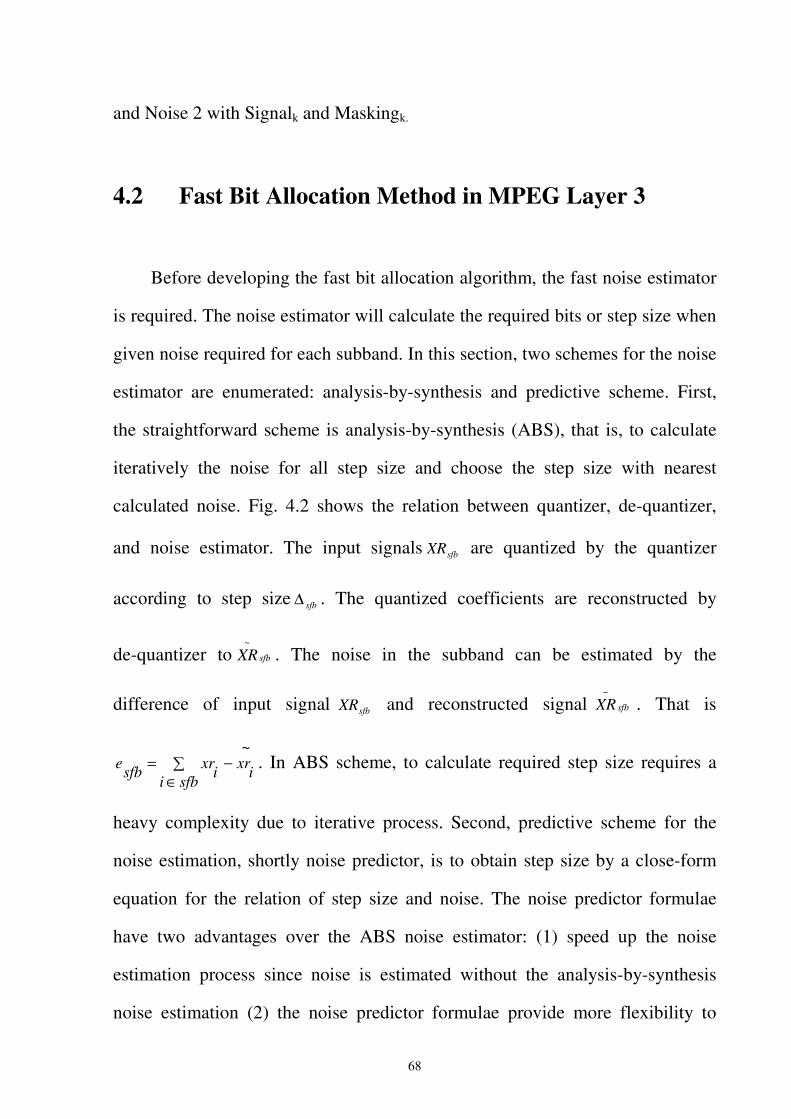
68

and Noise 2 with Signalk and Maskingk.

4.2 Fast Bit Allocation Method in MPEG Layer 3

Before developing the fast bit allocation algorithm, the fast noise estimator

is required. The noise estimator will calculate the required bits or step size when

given noise required for each subband. In this section, two schemes for the noise

estimator are enumerated: analysis-by-synthesis and predictive scheme. First,

the straightforward scheme is analysis-by-synthesis (ABS), that is, to calculate

iteratively the noise for all step size and choose the step size with nearest

calculated noise. Fig. 4.2 shows the relation between quantizer, de-quantizer,

and noise estimator. The input signals sfbXR are quantized by the quantizer

according to step size sfb∆ . The quantized coefficients are reconstructed by

de-quantizer to sfbXR~

. The noise in the subband can be estimated by the

difference of input signal sfbXR and reconstructed signal sfbXR~

. That is

�∈

−=sfbi

ixrixrsfbe~

. In ABS scheme, to calculate required step size requires a

heavy complexity due to iterative process. Second, predictive scheme for the

noise estimation, shortly noise predictor, is to obtain step size by a close-form

equation for the relation of step size and noise. The noise predictor formulae

have two advantages over the ABS noise estimator: (1) speed up the noise

estimation process since noise is estimated without the analysis-by-synthesis

noise estimation (2) the noise predictor formulae provide more flexibility to

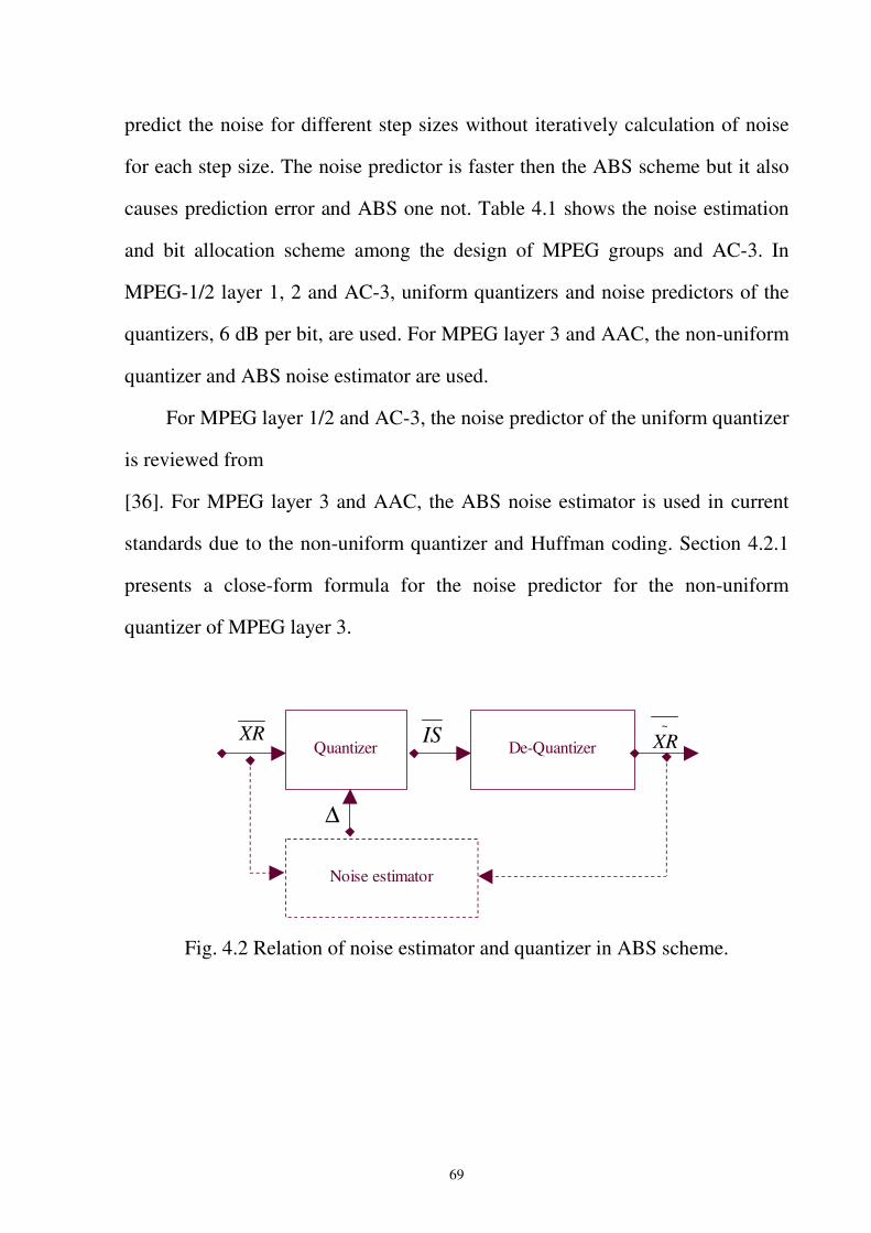
69

predict the noise for different step sizes without iteratively calculation of noise

for each step size. The noise predictor is faster then the ABS scheme but it also

causes prediction error and ABS one not. Table 4.1 shows the noise estimation

and bit allocation scheme among the design of MPEG groups and AC-3. In

MPEG-1/2 layer 1, 2 and AC-3, uniform quantizers and noise predictors of the

quantizers, 6 dB per bit, are used. For MPEG layer 3 and AAC, the non-uniform

quantizer and ABS noise estimator are used.

For MPEG layer 1/2 and AC-3, the noise predictor of the uniform quantizer

is reviewed from

[36]. For MPEG layer 3 and AAC, the ABS noise estimator is used in current

standards due to the non-uniform quantizer and Huffman coding. Section 4.2.1

presents a close-form formula for the noise predictor for the non-uniform

quantizer of MPEG layer 3.

Quantizer

De-Quantizer

XR ~

XRIS

Noise estimator

∆

Fig. 4.2 Relation of noise estimator and quantizer in ABS scheme.

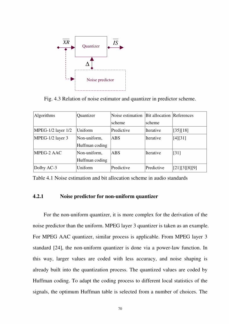
70

Quantizer

XR IS

Noise predictor

∆

Fig. 4.3 Relation of noise estimator and quantizer in predictor scheme.

Algorithms Quantizer Noise estimation

scheme

Bit allocation

scheme

References

MPEG-1/2 layer 1/2 Uniform Predictive Iterative [35][18]

MPEG-1/2 layer 3 Non-uniform,

Huffman coding

ABS Iterative [4][31]

MPEG-2 AAC Non-uniform,

Huffman coding

ABS Iterative [31]

Dolby AC-3 Uniform Predictive Predictive [21][3][8][9]

Table 4.1 Noise estimation and bit allocation scheme in audio standards

4.2.1 Noise predictor for non-uniform quantizer

For the non-uniform quantizer, it is more complex for the derivation of the

noise predictor than the uniform. MPEG layer 3 quantizer is taken as an example.

For MPEG AAC quantizer, similar process is applicable. From MPEG layer 3

standard [24], the non-uniform quantizer is done via a power-law function. In

this way, larger values are coded with less accuracy, and noise shaping is

already built into the quantization process. The quantized values are coded by

Huffman coding. To adapt the coding process to different local statistics of the

signals, the optimum Huffman table is selected from a number of choices. The

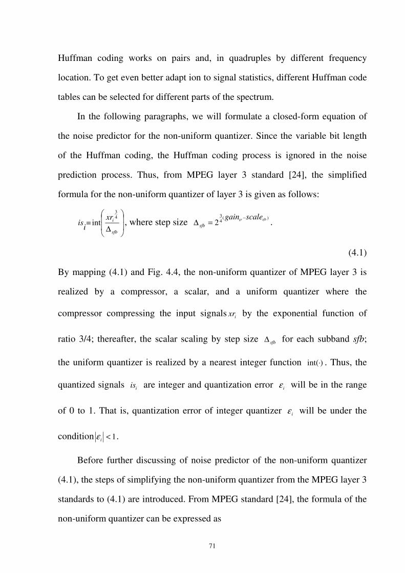
71

Huffman coding works on pairs and, in quadruples by different frequency

location. To get even better adapt ion to signal statistics, different Huffman code

tables can be selected for different parts of the spectrum.

In the following paragraphs, we will formulate a closed-form equation of

the noise predictor for the non-uniform quantizer. Since the variable bit length

of the Huffman coding, the Huffman coding process is ignored in the noise

prediction process. Thus, from MPEG layer 3 standard [24], the simplified

formula for the non-uniform quantizer of layer 3 is given as follows:

��

�

�

��

�

�

∆ sfb

ixr=iis

43

int , where step size )(43

2 sfbgr scalegainsfb

−=∆ .

(4.1)

By mapping (4.1) and Fig. 4.4, the non-uniform quantizer of MPEG layer 3 is

realized by a compressor, a scalar, and a uniform quantizer where the

compressor compressing the input signals ixr by the exponential function of

ratio 3/4; thereafter, the scalar scaling by step size sfb∆ for each subband sfb;

the uniform quantizer is realized by a nearest integer function )int(⋅ . Thus, the

quantized signals iis are integer and quantization error iε will be in the range

of 0 to 1. That is, quantization error of integer quantizer iε will be under the

condition 1<iε .

Before further discussing of noise predictor of the non-uniform quantizer

(4.1), the steps of simplifying the non-uniform quantizer from the MPEG layer 3

standards to (4.1) are introduced. From MPEG standard [24], the formula of the

non-uniform quantizer can be expressed as

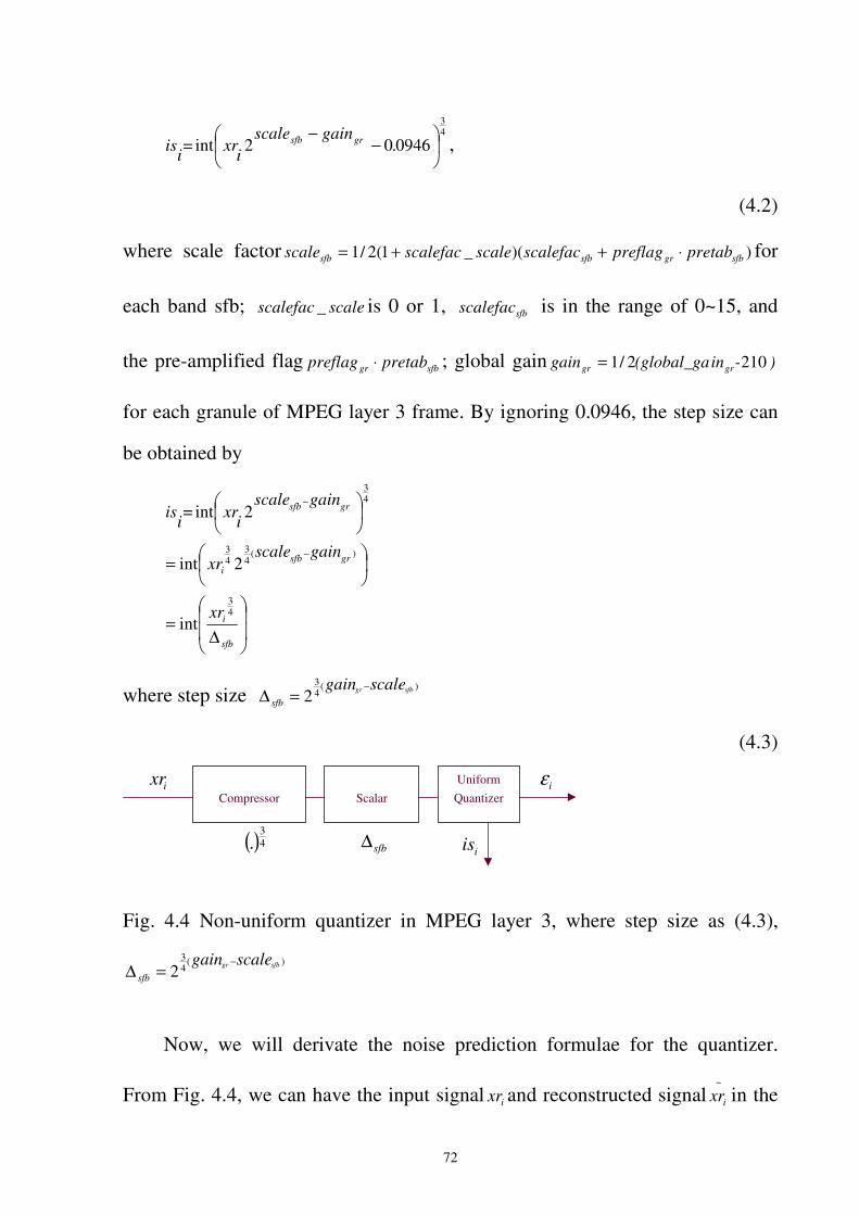
72

43

094602int ��

���

� −−

.gainscale

ixr=iis grsfb ,

(4.2)

where scale factor ))(_1(2/1 sfbgrsfbsfb pretabpreflagscalefacscalescalefacscale ⋅++= for

each band sfb; scalescalefac _ is 0 or 1, sfbscalefac is in the range of 0~15, and

the pre-amplified flag sfbgr pretabpreflag ⋅ ; global gain )-in(global_gagain grgr 2102/1=

for each granule of MPEG layer 3 frame. By ignoring 0.0946, the step size can

be obtained by

��

�

�

��

�

�

∆=

��

���

�=

��

���

�

−

−

sfb

i

grsfbi

grsfb

xr

gainscalexr

gainscaleixr=iis

43

)(43

43

43

int

2int

2int

where step size )(43

2 sfbgr scalegainsfb

−=∆

(4.3)

Uniform Quantizer

iis

iεixr Compressor

Scalar

( )43

. sfb∆

Fig. 4.4 Non-uniform quantizer in MPEG layer 3, where step size as (4.3),

)(43

2 sfbgr scalegainsfb

−=∆

Now, we will derivate the noise prediction formulae for the quantizer.

From Fig. 4.4, we can have the input signal ixr and reconstructed signal~

ixr in the

73

following two formulae.

( )34

sfbiii )�(isxr ε+=

(4.4)

and

( )34

sfbi

~

i �isxr = .

(4.5)

The quantization error of the non-uniform quantizer ie equal to the difference of

input signal ixr and ~

ixr . We will have

( ) ( ) ( )34

34

34

34

34

34 11 sfbisfbiiisfbisfbii

~

iii �is�is)is(�is)�(isxrxre −+=−+=−= − εε

(4.6)

From (4.6), by the definition of the function 3411) )�is(f(� iii

−+= , we can have the

quantization error in the form of

( )34

34

34

) sfbisfbii �is�isf(�e −= .

(4.7)

By Tylor expansion, we can have the first order approximation of ε)1) f'(�f(� +≈ .

13411

34 3

1

1) −−− ≈+= iiiii is)(is)�is(f'(�

(4.8)

We can have

iii �isf'(�f(� 1341)1) −+=+≈ ε

(4.9)

From (4.7), (4.8) and (4.9), the quantization error will be

74

( ) 34

31

34

34

34

34) sfbiisfbisfbiii �is�is�isf(�e ε≈−=

(4.10)

From (4.8) and assume quantized signals iis and quantized error of the uniform

quantizer iε are independent, we can have the expectation of quantization error

of the non-uniform quantizer ie as the follows:

]]E[E[IS�]E[IS�]E[ sfbsfbsfbsfbsfbsfbe 29

1629

162 32

38

32

38 εε ≈≈

(4.11)

According to

[36], the quantization error variance of uniform quantizer can be formulated as

12/22�=δ ; that is

12122 == ]E[ sfb�εδ , so the formula (4.11) becomes

]E[IS�]E[ sfbsfbsfbe 32

38

2742 ≈

(4.12)

By (4.5) and (4.12), the quantization error of the non-uniform quantizer is

]E[XR�]XR

E[�]E[ sfbsfbsfb

sfbsfbsfbe 2

1324

3

38 2

274

2742 )( =

∆≈

(4.13)

From (4.13), the signal-to-noise ratio can be expressed as

])E[XR�/XR(ESNR(dB) sfbsfbsfb212

2742

10 ][log10=

(4.14)

From (4.13), the noise predictor of the non-uniform quantizer depends not

only on the step size sfb∆ but also inputs signals sfbXR .

75

4.2.2 Fast bit allocation for non-uniform quantizer

From section 4.2.2, the noise predictor formulae of uniform and

non-uniform quantizer are given. Fast bit allocation can be developed by the

formulae. The noise predictor formula for uniform quantizer is widely adopted

in current design of audio standard. As shown in Table 4.1, all audio standards

using uniform quantizer, MPEG 1/2 layer 1, 2 and AC-3 use the noise predictor

formula to speed up the noise estimation process. Several papers [8][9][35][18]

propose fast algorithms on the uniform quantizer bit allocation on the basis on

the noise predictor formula.

From MPEG standard [24] and related papers [31], the original design of

the bit allocation is as following. A global gain that determines the quantization

step size and scalefactors that determine the noise-shaping factors for each

scalefactor band are applied before actual quantization. The process to find the

optimum gain and scalefactors for a given block, bit-rate and output from the

perceptual model is usually done by two nested iteration loops in an

analysis-by-synthesis way. (1) Inner iteration loop (rate loop): If the number of

bits resulting from the coding operation exceeds the number of bits available to

code a given block of data, this can be corrected by adjusting the global gain to

result in a larger quantization step size, leading to smaller quantized values. This

operation is repeated with different quantization step sizes until the resulting bit

demand for Huffman coding is small enough. (2) Outer iteration loop (noise

control loop): To shape the quantization noise according to the masking

threshold, scalefactors are applied to each scalefactor band. If the quantization

noise in a given band is found to exceed the masking threshold as supplied by

76

the perceptual model, the scalefactor for this band is adjusted to reduce the

quantization noise. Since achieving a smaller quantization noise requires a larger

number of quantization steps and thus a higher bit-rate, the rate adjustment loop

has to be repeated every time new scalefactors are used. The two nested loops

ensure the demand of bit rate and noise shaping for each subband by iteratively

using analysis-by-synthesis noise estimator. A new fast bit allocation algorithm

based on the noise predictor formula presented in 4.2.1 is proposed. The new bit

allocation also meets the demand of bit rate and noise shaping for each subband

by single step prediction.

From

[44], the perceptual optimal solution for subband bit allocation is the quantized

noise for each subband should be a ratio to masking threshold 2sfbThr . That is the

expected noise will be

22 ][ sfbsfb ThrceE ⋅=

(4.15)

where c is a constant varied with bit rate. According to (4.13), substituting (4.15)

into (4.13), we can obtain

]E[XR�Thrc]E[e sfbsfbsfbsfb2/12

27422 ≈⋅= ,

or in the form of

]E[XRThrc� sfbsfbsfb2/12

4272 /⋅≈

(4.16)

According to (4.1) for the step size, we can have

77

]/2 2/12427)(2 2

3

sfbsfbscalegain

sfb E[XRThrc�sfbgr ⋅≈= −

(4.17)

From (4.17), the difference of global gain and scalefactor is approximate to

]/log 2/124

2723

2sfbsfbsfbgr E[XRThrcscalegain ⋅≈− ,

or in the form of

)(scalegain ]E[XRThrcsfbgr

sfbsfb2/12

427

222232 loglogloglog −++=−

(4.18)

Since scalefactor sfbscale is in the range of 0~31. To obtain scalefactor for each

subband, let { }sfbgrsfb

gr scalegainMaxgain −=' . The scalefactor for each subband will

be

sfbgrsfb scalegainscale −= '' .

(4.19)

Reordering the formula (4.18) and substituting the resulting scalefactor from

(4.19) yields

)log(logloglog'2/12

427

2232

2232 ]E[XRThrc

sfbgrsfbsfb)(scalegain −++=− .

(4.20)

From (4.20), the global gain grgain varies with the bit rate related constant c and

scalefactor sfbscale varies for each subband according to the masking threshold

2sfbThr and input signals ][ 2/1

sfbXRE .

The experiment results are given for the fast allocation. In Fig. 4.5, the

Noise curve for the original MPEG bit allocation and proposed algorithm are

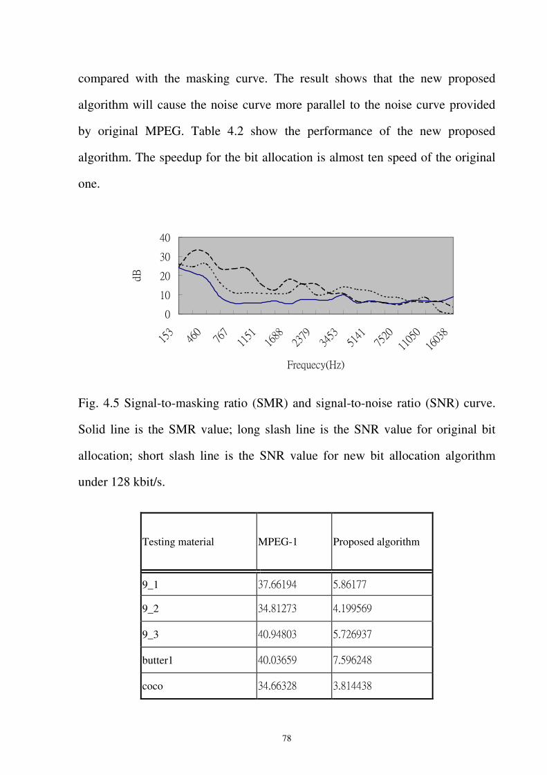
78

compared with the masking curve. The result shows that the new proposed

algorithm will cause the noise curve more parallel to the noise curve provided

by original MPEG. Table 4.2 show the performance of the new proposed

algorithm. The speedup for the bit allocation is almost ten speed of the original

one.

Fig. 4.5 Signal-to-masking ratio (SMR) and signal-to-noise ratio (SNR) curve.

Solid line is the SMR value; long slash line is the SNR value for original bit

allocation; short slash line is the SNR value for new bit allocation algorithm

under 128 kbit/s.

Testing material MPEG-1 Proposed algorithm

9_1

9_2

9_3

butter1

coco

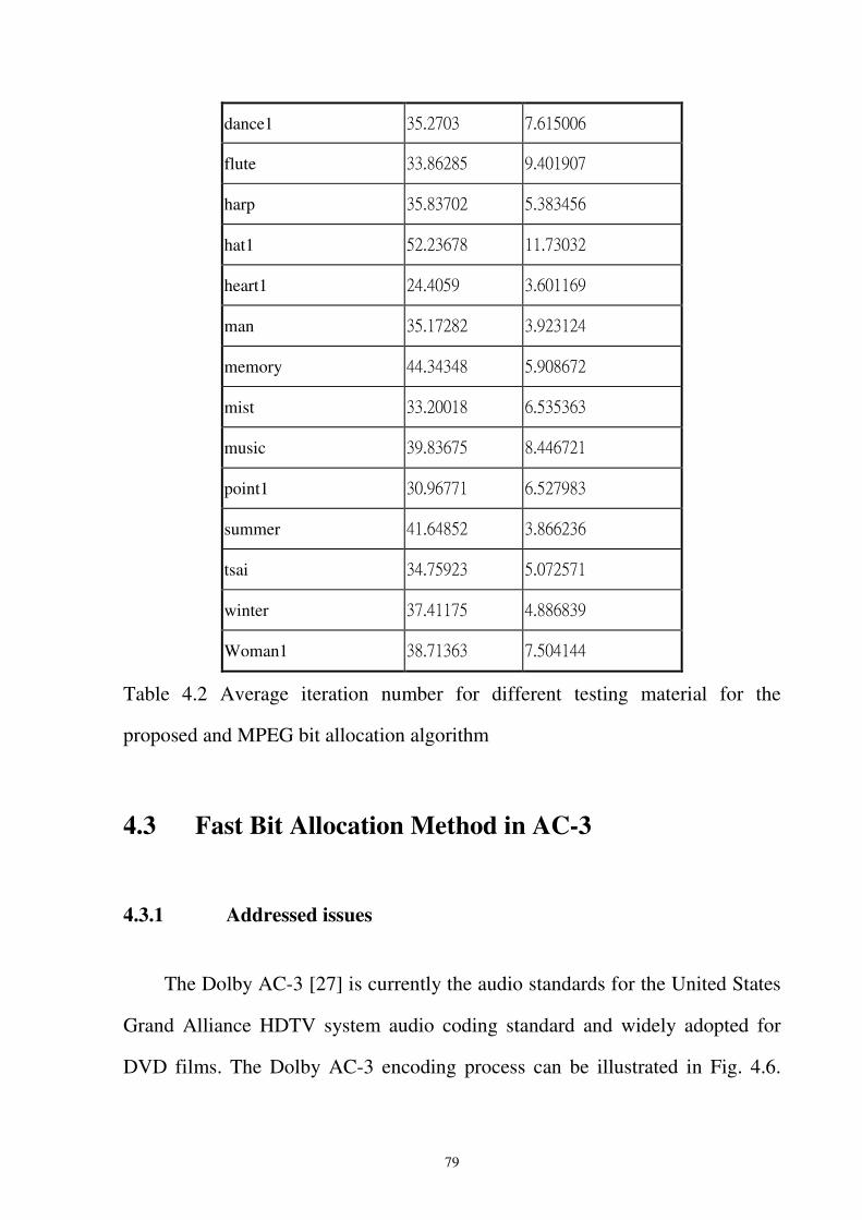
79

dance1

flute

harp

hat1

heart1

man

memory

mist

music

point1

summer

tsai

winter

Woman1

Table 4.2 Average iteration number for different testing material for the

proposed and MPEG bit allocation algorithm

4.3 Fast Bit Allocation Method in AC-3

4.3.1 Addressed issues

The Dolby AC-3 [27] is currently the audio standards for the United States

Grand Alliance HDTV system audio coding standard and widely adopted for

DVD films. The Dolby AC-3 encoding process can be illustrated in Fig. 4.6.

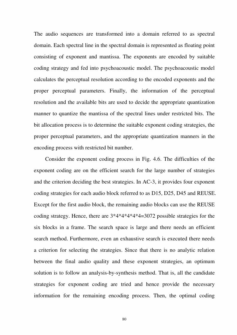
80

The audio sequences are transformed into a domain referred to as spectral

domain. Each spectral line in the spectral domain is represented as floating point

consisting of exponent and mantissa. The exponents are encoded by suitable

coding strategy and fed into psychoacoustic model. The psychoacoustic model

calculates the perceptual resolution according to the encoded exponents and the

proper perceptual parameters. Finally, the information of the perceptual

resolution and the available bits are used to decide the appropriate quantization

manner to quantize the mantissa of the spectral lines under restricted bits. The

bit allocation process is to determine the suitable exponent coding strategies, the

proper perceptual parameters, and the appropriate quantization manners in the

encoding process with restricted bit number.

Consider the exponent coding process in Fig. 4.6. The difficulties of the

exponent coding are on the efficient search for the large number of strategies

and the criterion deciding the best strategies. In AC-3, it provides four exponent

coding strategies for each audio block referred to as D15, D25, D45 and REUSE.

Except for the first audio block, the remaining audio blocks can use the REUSE

coding strategy. Hence, there are 3*4*4*4*4*4=3072 possible strategies for the

six blocks in a frame. The search space is large and there needs an efficient

search method. Furthermore, even an exhaustive search is executed there needs

a criterion for selecting the strategies. Since that there is no analytic relation

between the final audio quality and these exponent strategies, an optimum

solution is to follow an analysis-by-synthesis method. That is, all the candidate

strategies for exponent coding are tried and hence provide the necessary

information for the remaining encoding process. Then, the optimal coding

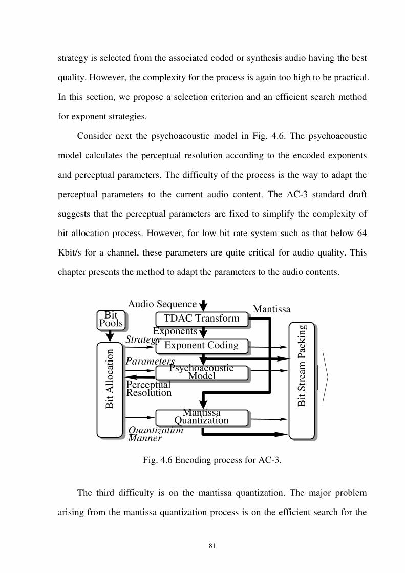
81

strategy is selected from the associated coded or synthesis audio having the best

quality. However, the complexity for the process is again too high to be practical.

In this section, we propose a selection criterion and an efficient search method

for exponent strategies.

Consider next the psychoacoustic model in Fig. 4.6. The psychoacoustic

model calculates the perceptual resolution according to the encoded exponents

and perceptual parameters. The difficulty of the process is the way to adapt the

perceptual parameters to the current audio content. The AC-3 standard draft

suggests that the perceptual parameters are fixed to simplify the complexity of

bit allocation process. However, for low bit rate system such as that below 64

Kbit/s for a channel, these parameters are quite critical for audio quality. This

chapter presents the method to adapt the parameters to the audio contents.

TDAC Transform TDAC Transform

Audio Sequence

Exponent Coding Exponent Coding

Psychoacoustic Model

Mantissa Quantization

Mantissa Quantization

Mantissa

Exponents

Bit

Allo

catio

n B

it A

lloca

tion

Strategy

Parameters

Bit Pools Bit

Pools

Perceptual Resolution

Bit

Stre

am P

acki

ng

Bit

Stre

am P

acki

ng

Quantization Manner

Fig. 4.6 Encoding process for AC-3.

The third difficulty is on the mantissa quantization. The major problem

arising from the mantissa quantization process is on the efficient search for the

82

value of quantization parameter provided by the AC-3 to fit the available bits. In

AC-3, the mantissa quantization process is to quantize the mantissa of each

spectral line according to the perceptual resolution and the values of

quantization parameter. There are 1024 selections for the parameter in AC-3 and

a vehicle searching for the optimal value fitting the restricted bits is needed. The

problem is that there is no direct relation among the values of the parameter, the

perceptual resolution, and the available bits. That is, there is no way finding the

suitable quantization value directly from the perceptual resolution and the

available bits. This section proposes the efficient algorithm for searching the

optimal value of the quantization parameter in AC-3.

The rest of this section is organized as follows: Section 4.3.2 illustrates the

efficient searching algorithm and selection criteria for exponent coding process.

Section 4.3.3 provides the method to adapt the perceptual parameters to current

audio content and also gives the efficient searching algorithm for the

quantization parameter. Section 4.3.4 shows the experiment results. Section

4.3.5 gives a brief conclusion.

4.3.2 Exponent coding method

In AC-3, each spectral line is represented by an exponent and a mantissa.

All the exponents are coded by the exponent coding process. The coding

strategies available in AC-3 are referred to as D15, D25, D45 and REUSE. The

coding strategy D15 provides the finest frequency resolution and hence requires

a large number of bits. On the contrary, the strategy D45 gives the coarsest

frequency resolution and hence consumes a less number of bits. Especially, the

83

strategy REUSE indicates that the exponents of current block are the same as the

previous block and hence there is no bit requirement for the exponent of current

audio block.

As described in last section, two difficulties on the exponent coding are the

large combinational space of the exponent coding strategies and the selection

criterion. This section proposes a selection criterion and the associated efficient

search method for the exponent strategies. The block diagram of the exponent

coding process is illustrated in Fig. 4.7. The process consists of three steps. First,

the available bits of the exponents are determined from the current bit rate. A

ratio of 20% of the overall bit rate has been adopted to select the exponent

strategies. The ratio has been determined through immense experiments. On the

ratio, the second step is to list all the exponent strategies that consume a bit

number less than the available bits. For music sequence adopting a fixed frame

rate, the candidates are fixed and will not vary with frames. Finally, all the

candidates are used to encode the exponents. On all the associated encoded

exponents, the strategy that minimizes the error criterion is selected. The error

criterion is listed as follows:

[ ]��= =

−=5

0

255

0

),exp(),(expk b

o bkbkE

(4.21)

where expo(k,b) is the original exponent of block k and spectral bin b before

encoding, and exp(k,b) is the corresponding exponent encoded by a candidate

strategy. In a frame defined by AC-3, there are six blocks and 256 spectral bins

in a block. The criterion is reasonable in the sense that the formula indicates the

error between the coded and the original exponents. The overall process can find

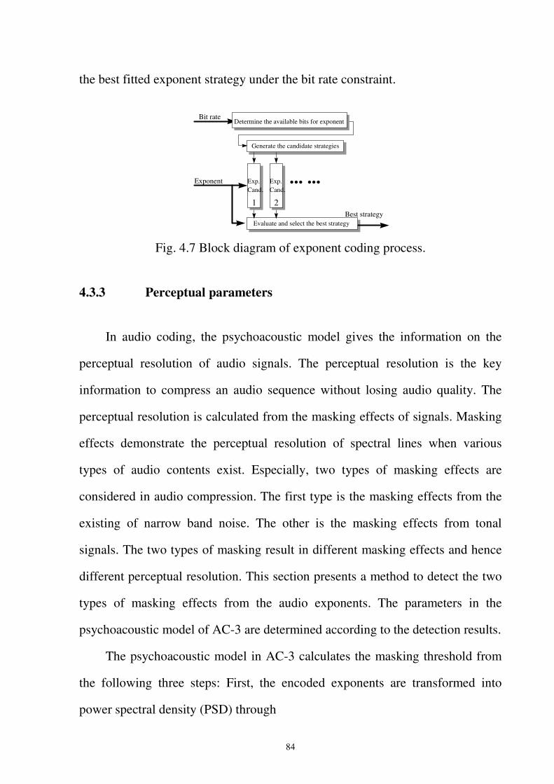
84

the best fitted exponent strategy under the bit rate constraint.

Bit rate

Generate the candidate strategies Generate the candidate strategies

... ...

Evaluate and select the best strategy Evaluate and select the best strategy

Exponent

Best strategy

Determine the available bits for exponent

Exp.Cand.

Exp.Cand.

1 2

Fig. 4.7 Block diagram of exponent coding process.

4.3.3 Perceptual parameters

In audio coding, the psychoacoustic model gives the information on the

perceptual resolution of audio signals. The perceptual resolution is the key

information to compress an audio sequence without losing audio quality. The

perceptual resolution is calculated from the masking effects of signals. Masking

effects demonstrate the perceptual resolution of spectral lines when various

types of audio contents exist. Especially, two types of masking effects are

considered in audio compression. The first type is the masking effects from the

existing of narrow band noise. The other is the masking effects from tonal

signals. The two types of masking result in different masking effects and hence

different perceptual resolution. This section presents a method to detect the two

types of masking effects from the audio exponents. The parameters in the

psychoacoustic model of AC-3 are determined according to the detection results.

The psychoacoustic model in AC-3 calculates the masking threshold from

the following three steps: First, the encoded exponents are transformed into

power spectral density (PSD) through

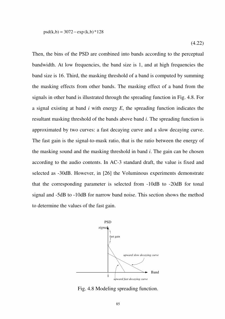
85

128*b)(k, exp3072b)psd(k, −=

(4.22)

Then, the bins of the PSD are combined into bands according to the perceptual

bandwidth. At low frequencies, the band size is 1, and at high frequencies the

band size is 16. Third, the masking threshold of a band is computed by summing

the masking effects from other bands. The masking effect of a band from the

signals in other band is illustrated through the spreading function in Fig. 4.8. For

a signal existing at band i with energy E, the spreading function indicates the

resultant masking threshold of the bands above band i. The spreading function is

approximated by two curves: a fast decaying curve and a slow decaying curve.

The fast gain is the signal-to-mask ratio, that is the ratio between the energy of

the masking sound and the masking threshold in band i. The gain can be chosen

according to the audio contents. In AC-3 standard draft, the value is fixed and

selected as -30dB. However, in [26] the Voluminous experiments demonstrate

that the corresponding parameter is selected from -10dB to -20dB for tonal

signal and -5dB to -10dB for narrow band noise. This section shows the method

to determine the values of the fast gain.

signal

upward slow decaying curve

Band

PSD

fast gain

upward fast decaying curve i

Fig. 4.8 Modeling spreading function.

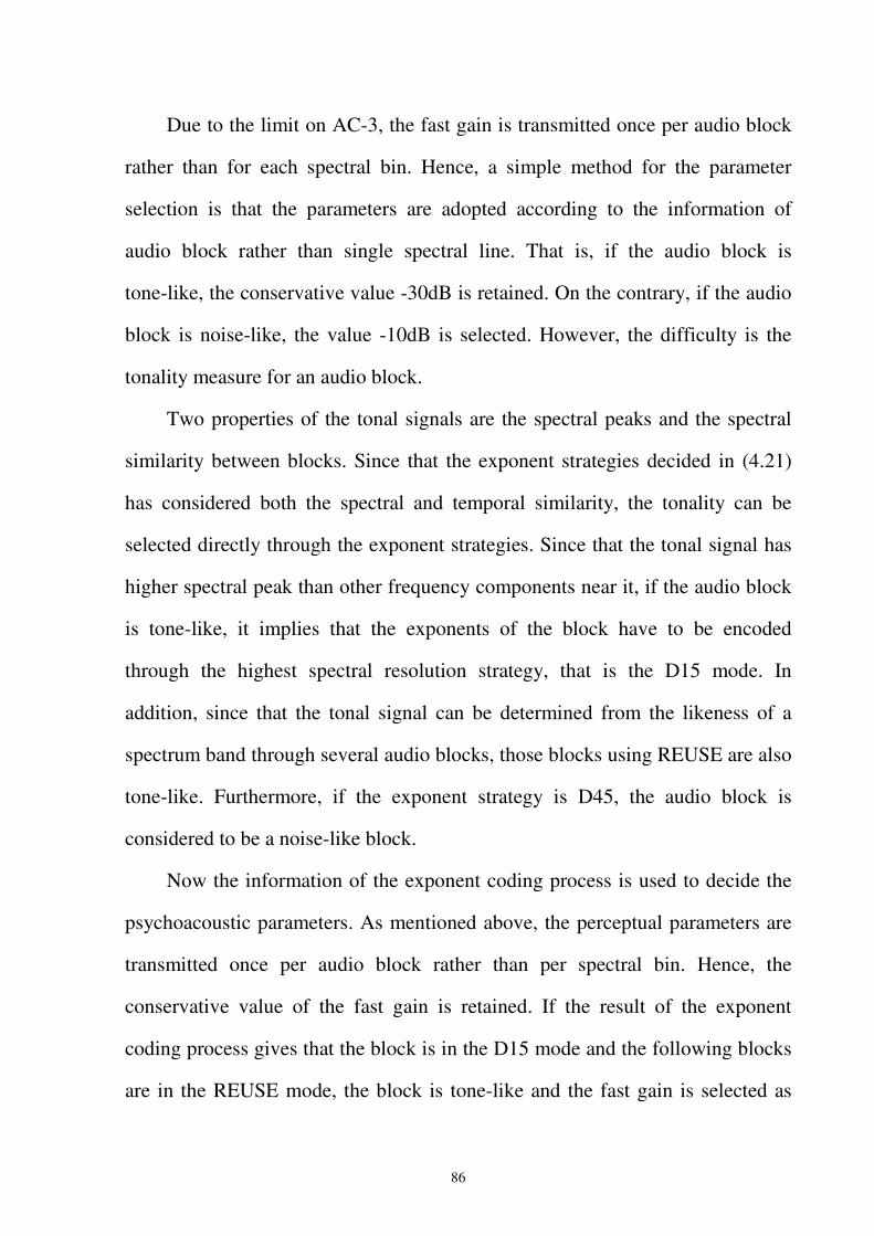
86

Due to the limit on AC-3, the fast gain is transmitted once per audio block

rather than for each spectral bin. Hence, a simple method for the parameter

selection is that the parameters are adopted according to the information of

audio block rather than single spectral line. That is, if the audio block is

tone-like, the conservative value -30dB is retained. On the contrary, if the audio

block is noise-like, the value -10dB is selected. However, the difficulty is the

tonality measure for an audio block.

Two properties of the tonal signals are the spectral peaks and the spectral

similarity between blocks. Since that the exponent strategies decided in (4.21)

has considered both the spectral and temporal similarity, the tonality can be

selected directly through the exponent strategies. Since that the tonal signal has

higher spectral peak than other frequency components near it, if the audio block

is tone-like, it implies that the exponents of the block have to be encoded

through the highest spectral resolution strategy, that is the D15 mode. In

addition, since that the tonal signal can be determined from the likeness of a

spectrum band through several audio blocks, those blocks using REUSE are also

tone-like. Furthermore, if the exponent strategy is D45, the audio block is

considered to be a noise-like block.

Now the information of the exponent coding process is used to decide the

psychoacoustic parameters. As mentioned above, the perceptual parameters are

transmitted once per audio block rather than per spectral bin. Hence, the

conservative value of the fast gain is retained. If the result of the exponent

coding process gives that the block is in the D15 mode and the following blocks

are in the REUSE mode, the block is tone-like and the fast gain is selected as

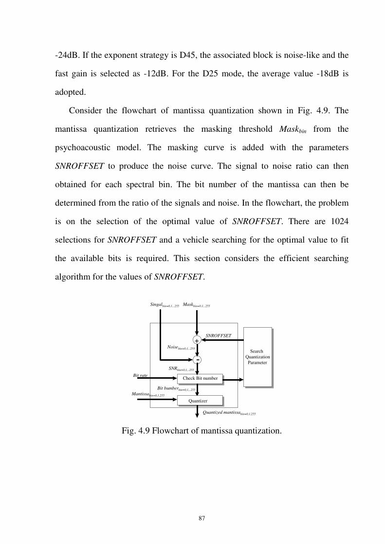
87

-24dB. If the exponent strategy is D45, the associated block is noise-like and the

fast gain is selected as -12dB. For the D25 mode, the average value -18dB is

adopted.

Consider the flowchart of mantissa quantization shown in Fig. 4.9. The

mantissa quantization retrieves the masking threshold Maskbin from the

psychoacoustic model. The masking curve is added with the parameters

SNROFFSET to produce the noise curve. The signal to noise ratio can then

obtained for each spectral bin. The bit number of the mantissa can then be

determined from the ratio of the signals and noise. In the flowchart, the problem

is on the selection of the optimal value of SNROFFSET. There are 1024

selections for SNROFFSET and a vehicle searching for the optimal value to fit

the available bits is required. This section considers the efficient searching

algorithm for the values of SNROFFSET.

Maskbin=0,1,..255

SNROFFSET+

Noisebin=0,1,..255

-

Singalbin=0,1,..255

SNRbin=0,1,..255

Quantizer

Bit bumberbin=0,1,..255

Bit rate

Mantissabin=0,1,255

Quantized mantissabin=0,1,255

SearchQuantization Parameter

Check Bit number

Fig. 4.9 Flowchart of mantissa quantization.

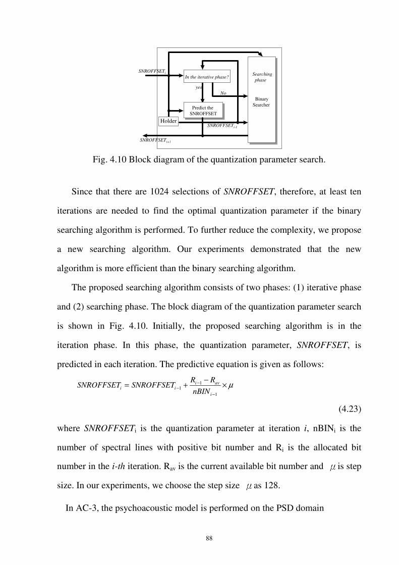
88

No

In the iterative phase?SNROFFSETi

SNROFFSETi-1

yes

Predict the SNROFFSET

SNROFFSETi+1

Holder

Binary Searcher

Searching phase

Fig. 4.10 Block diagram of the quantization parameter search.

Since that there are 1024 selections of SNROFFSET, therefore, at least ten

iterations are needed to find the optimal quantization parameter if the binary

searching algorithm is performed. To further reduce the complexity, we propose

a new searching algorithm. Our experiments demonstrated that the new

algorithm is more efficient than the binary searching algorithm.

The proposed searching algorithm consists of two phases: (1) iterative phase

and (2) searching phase. The block diagram of the quantization parameter search

is shown in Fig. 4.10. Initially, the proposed searching algorithm is in the

iteration phase. In this phase, the quantization parameter, SNROFFSET, is

predicted in each iteration. The predictive equation is given as follows:

µ×−+=−

−−

1

11

i

aviii nBIN

RRSNROFFSETSNROFFSET

(4.23)

where SNROFFSETi is the quantization parameter at iteration i, nBINi is the

number of spectral lines with positive bit number and Ri is the allocated bit

number in the i-th iteration. Rav is the current available bit number and is step

size. In our experiments, we choose the step size as 128.

In AC-3, the psychoacoustic model is performed on the PSD domain

89

[3]. The PSD is derived by the encoded exponent expressed in (4.22). Hence, the

PSD-decibel has the following relation:

dB 6 PSDunits 128 =

(4.24)

From

[36], since that additional one bit resolution increases the signal-to-noise ratio by

6dB for uniform quantizers, the signal-to-noise ratio is increased by 128 units

PSD. Therefore, the step size is chosen as 128. In the low bit rate system, the

symmetric quantizers are often used. In the condition, the step size has to be

decreased to avoid over-prediction.

The iteration terminates when the following two conditions are met: (a) Ri

Rav, Ri-1>Rav or (b) Ri-1 Rav, Ri>Rav. The search phase then searches the

optimal value from the range between SNROFFSETi and SNROFFSETi-1 by the

binary search algorithm. Since that the optimal quantization parameter is

bounded by SNROFFSETi and SNROFFSETi-1 which is the sub-region of 0 to

1024, the binary searching algorithm takes less than ten iterations to find the

optimal value of SNROFFSET.

source butter tsai dance flute heart1 memory second march Russian Chinese

count 5.18 5.81 4.94 4.91 6.02 5.78 6.09 5.40 5.86 4.25

Table 4.3 Average iteration counts per frame.

4.3.4 Experiment results

This section considers the efficiency of the encoding algorithm. In the

90

following experiments, each audio channel is encoded at the bit rate of 64 Kbit/s

with sampling frequency of 44.1 KHz. The bit number of the exponents is 435 in

one frame. The exponents coding strategies that consume less than 20% frame

bit rate are listed in Table 4.4. The three audio sequences illustrated in Fig. 4.11

can provide a typical example for the experiments. The decided exponent coding

strategy also decides the tonality of the block. Fig. 4.11 illustrates three

examples of the tonality decision. The decisions are quite consistent with audio

contents.

For the experiments on searching the values of the SNROFFSET, a total of

ten 20 sec stereo audio songs including vocal, symphony, piano and so on are

taken as the materials. Table 4.3 lists the average iteration numbers per frame of

mantissa quantization for above materials. The iteration numbers demonstrate

that the proposed method provides an iteration number much lower than ten that

is the iteration counts of binary searches for 1024 values.

(1) [D15,REUSE,REUSE,REUSE,REUSE,REUSE]

(2) [D25,REUSE, REUSE,D25,REUSE,REUSE]

(3) [D25,REUSE,REUSE,D45, REUSE,D45]

(4) [D25,REUSE,D45,REUSE,D45, REUSE]

(5) [D45,D45,REUSE,D45, REUSE,D45]

Table 4.4 Candidates of exponent coding strategies.

4.3.5 Remarks

In AC-3 encoder, the bit allocation is quite computation intensive and there

is no article analyzing the problem. This section has analyzed the problem and

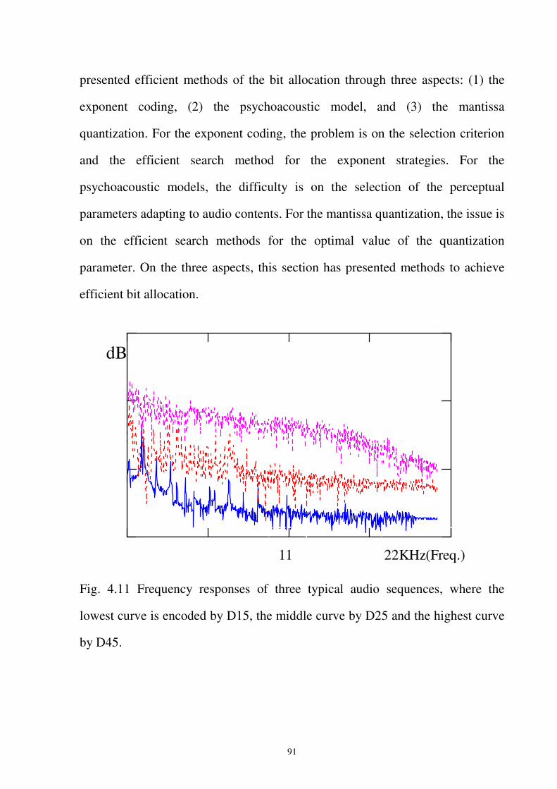
91

presented efficient methods of the bit allocation through three aspects: (1) the

exponent coding, (2) the psychoacoustic model, and (3) the mantissa

quantization. For the exponent coding, the problem is on the selection criterion

and the efficient search method for the exponent strategies. For the

psychoacoustic models, the difficulty is on the selection of the perceptual

parameters adapting to audio contents. For the mantissa quantization, the issue is

on the efficient search methods for the optimal value of the quantization

parameter. On the three aspects, this section has presented methods to achieve

efficient bit allocation.

dB

22KHz(Freq.) 11

Fig. 4.11 Frequency responses of three typical audio sequences, where the

lowest curve is encoded by D15, the middle curve by D25 and the highest curve

by D45.

92

4.4 Concluding Remarks

In this chapter, fast algorithms for bit allocation is addressed. The fast

algorithm for bit allocation is based on the fast noise estimator. The fast noise

estimator, not using the ABS noise estimator to iteratively calculate the noise of

each step sizes, provides a close-form equation for the relation of bits/step size

and quantization noise. With the noise prediction formulae of uniform or

non-uniform quantizer, several speedup algorithms are proposed in different

papers. In this dissertation, the non-uniform quantizer of MPEG layer 3 is taken

as an example. A single step bit allocation ensuring the criteria of maximal

perceptual coding gain for this quantizer is proposed and it is also applicable to

MPEG AAC non-uniform quantizer.

93

Chapter 5 KL Transform for Intensity/Coupling Coding

5.1 Introduction

When the two channels of stereo signals are coded, the stereo irrelevancy

for the two channels expresses that the ability of the human auditory system to

resolve the exact location of audio sources decreases with frequency. As stated

in [17] and [29], the localization of the stereophonic image for the frequencies

above 2 kHz is determined by the signal envelope instead of the signal fine

structures. Following the stereo irrelevancy, the audio standards have developed

the coupling or intensity schemes to efficiently remove the irrelevancy. Table

5.1 gives a summary on the coupling/intensity schemes in these audio coding

standards.

In this chapter, KL (Karhunen-Loève) transform is introduced to design

and analyze the intensity/coupling schemes. When integrating the KL transform

into intensity coding/coupling schemes of MPEG and AC-3, two issues arise.

The first issue lies on KL transform for intensity/coupling scheme might not

perceptually optimal even if it is optimal in numerical sense. Second, due to the

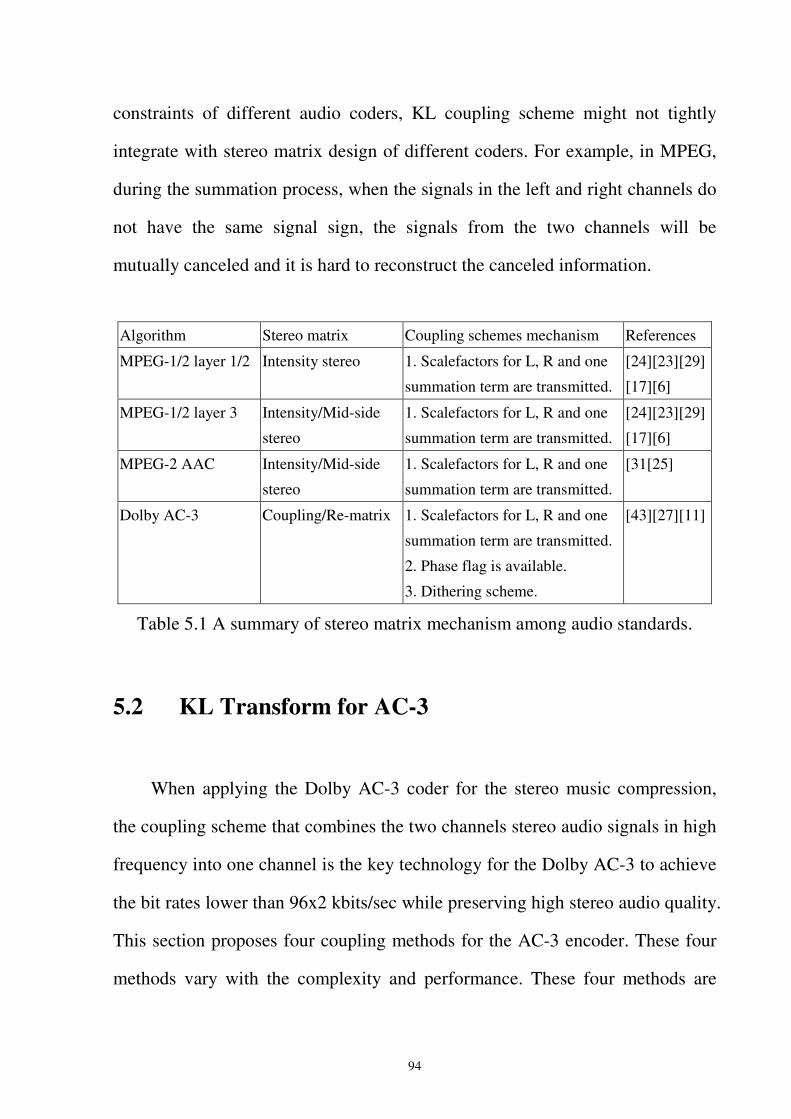
94

constraints of different audio coders, KL coupling scheme might not tightly

integrate with stereo matrix design of different coders. For example, in MPEG,

during the summation process, when the signals in the left and right channels do

not have the same signal sign, the signals from the two channels will be

mutually canceled and it is hard to reconstruct the canceled information.

Algorithm Stereo matrix Coupling schemes mechanism References

MPEG-1/2 layer 1/2 Intensity stereo 1. Scalefactors for L, R and one

summation term are transmitted.

[24][23][29]

[17][6]

MPEG-1/2 layer 3 Intensity/Mid-side

stereo

1. Scalefactors for L, R and one

summation term are transmitted.

[24][23][29]

[17][6]

MPEG-2 AAC Intensity/Mid-side

stereo

1. Scalefactors for L, R and one

summation term are transmitted.

[31[25]

Dolby AC-3 Coupling/Re-matrix 1. Scalefactors for L, R and one

summation term are transmitted.

2. Phase flag is available.

3. Dithering scheme.

[43][27][11]

Table 5.1 A summary of stereo matrix mechanism among audio standards.

5.2 KL Transform for AC-3

When applying the Dolby AC-3 coder for the stereo music compression,

the coupling scheme that combines the two channels stereo audio signals in high

frequency into one channel is the key technology for the Dolby AC-3 to achieve

the bit rates lower than 96x2 kbits/sec while preserving high stereo audio quality.

This section proposes four coupling methods for the AC-3 encoder. These four

methods vary with the complexity and performance. These four methods are

95

compared through both subjective and objective tests. These four coupling

methods are also combined with the dithering scheme and examined through

subjective and objective tests. The result shows that the dithering scheme can

effectively ease the coupling artifacts and enhance the audio quality.

5.2.1 Addressed issues

The coupling scheme, which applies the low perceptual sensitivity of the

stereo signals in high frequency to audio compression, is the key technology to

achieve near transparent quality at the bit rates below 96x2 kbits/sec. The

principle of the coupling scheme is derived from the stereo irrelevancy from the

auditory systems. The stereo irrelevancy expresses that the ability of the human

auditory system to resolve the exact location of audio sources decreases with

frequency. As stated in [17] and [29], the localization of the stereophonic image

for the frequencies above 2 kHz is determined by the signal envelope instead of

the signal fine structures. Following the stereo irrelevancy, the AC-3 coder has

developed the coupling scheme to achieve efficient compression. However, the

standard draft [27] illustrates the decoupling process for the decoder and leaves

unmentioned the coupling process for the encoder. This section proposes and

compares four coupling methods for the coupling process of the AC-3 encoder.

Fig. 5.1 illustrates the block diagram for the coupling process in the Dolby

AC-3. The audio sequences in stereo signal pairs are individually transformed

into spectral lines and grouped into vectors referred to as the coupling bands. Fig.

5.1 shows the coupling process for one band corresponding to the same

frequency range in a stereo signal pair. The bands from the left and the right

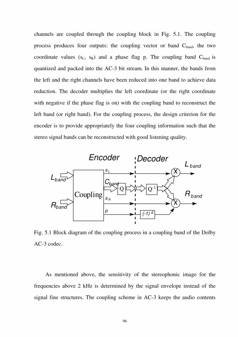
96

channels are coupled through the coupling block in Fig. 5.1. The coupling

process produces four outputs: the coupling vector or band Cband, the two

coordinate values (sL, sR) and a phase flag p. The coupling band Cband is

quantized and packed into the AC-3 bit stream. In this manner, the bands from

the left and the right channels have been reduced into one band to achieve data

reduction. The decoder multiplies the left coordinate (or the right coordinate

with negative if the phase flag is on) with the coupling band to reconstruct the

left band (or right band). For the coupling process, the design criterion for the

encoder is to provide appropriately the four coupling information such that the

stereo signal bands can be reconstructed with good listening quality.

L band

R band

Q

Encoder Decoder

Q -1

s L

s R

C band

x

x Coupling R band

(-1) p

L band

p

Fig. 5.1 Block diagram of the coupling process in a coupling band of the Dolby

AC-3 codec.

As mentioned above, the sensitivity of the stereophonic image for the

frequencies above 2 kHz is determined by the signal envelope instead of the

signal fine structures. The coupling scheme in AC-3 keeps the audio contents

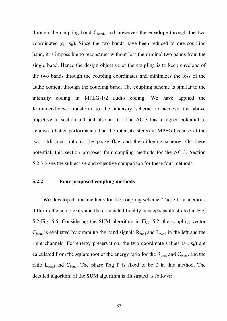
97

through the coupling band Cband, and preserves the envelope through the two

coordinates (sL, sR). Since the two bands have been reduced to one coupling

band, it is impossible to reconstruct without loss the original two bands from the

single band. Hence the design objective of the coupling is to keep envelope of

the two bands through the coupling coordinates and minimizes the loss of the

audio content through the coupling band. The coupling scheme is similar to the

intensity coding in MPEG-1/2 audio coding. We have applied the

Karhuner-Loeve transform to the intensity scheme to achieve the above

objective in section 5.3 and also in [6]. The AC-3 has a higher potential to

achieve a better performance than the intensity stereo in MPEG because of the

two additional options: the phase flag and the dithering scheme. On these

potential, this section proposes four coupling methods for the AC-3. Section

5.2.3 gives the subjective and objective comparison for these four methods.

5.2.2 Four proposed coupling methods

We developed four methods for the coupling scheme. These four methods

differ in the complexity and the associated fidelity concepts as illustrated in Fig.

5.2-Fig. 5.5. Considering the SUM algorithm in Fig. 5.2, the coupling vector

Cband is evaluated by summing the band signals Rband and Lband in the left and the

right channels. For energy preservation, the two coordinate values (sL, sR) are

calculated from the square root of the energy ratio for the Rband and Cband, and the

ratio Lband and Cband. The phase flag P is fixed to be 0 in this method. The

detailed algorithm of the SUM algorithm is illustrated as follows:

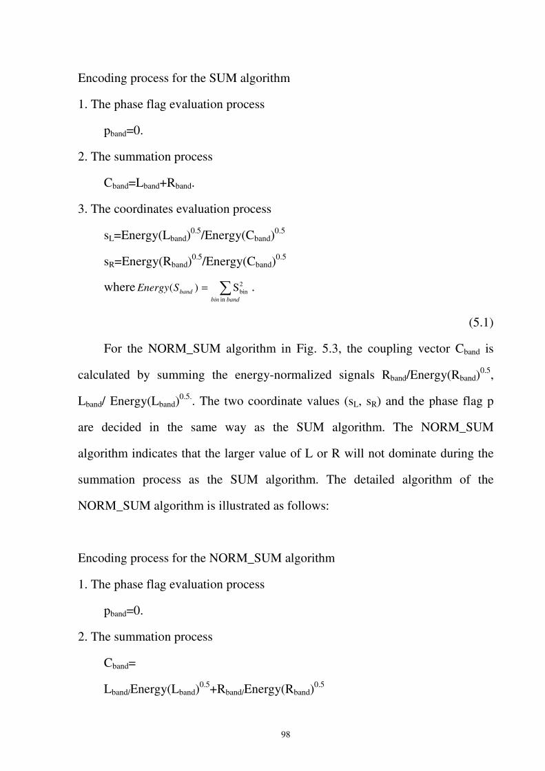
98

Encoding process for the SUM algorithm

1. The phase flag evaluation process

pband=0.

2. The summation process

Cband=Lband+Rband.

3. The coordinates evaluation process

sL=Energy(Lband)0.5/Energy(Cband)

0.5

sR=Energy(Rband)0.5/Energy(Cband)

0.5

where �=bandbin

bandSEnergyin

2binS)( .

(5.1)

For the NORM_SUM algorithm in Fig. 5.3, the coupling vector Cband is

calculated by summing the energy-normalized signals Rband/Energy(Rband)0.5,

Lband/ Energy(Lband)0.5.. The two coordinate values (sL, sR) and the phase flag p

are decided in the same way as the SUM algorithm. The NORM_SUM

algorithm indicates that the larger value of L or R will not dominate during the

summation process as the SUM algorithm. The detailed algorithm of the

NORM_SUM algorithm is illustrated as follows:

Encoding process for the NORM_SUM algorithm

1. The phase flag evaluation process

pband=0.

2. The summation process

Cband=

Lband/Energy(Lband)0.5+Rband/Energy(Rband)

0.5

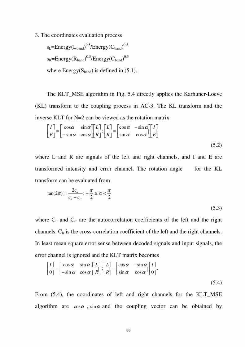
99

3. The coordinates evaluation process

sL=Energy(Lband)0.5/Energy(Cband)

0.5

sR=Energy(Rband)0.5/Energy(Cband)

0.5

where Energy(Sband) is defined in (5.1).

The KLT_MSE algorithm in Fig. 5.4 directly applies the Karhuner-Loeve

(KL) transform to the coupling process in AC-3. The KL transform and the

inverse KLT for N=2 can be viewed as the rotation matrix

��

�

��

�

−=

��

�

R

L

E

I

αααα

cossinsincos

;

��

�

��

� −=

��

�

E

I

R

L

αααα

cossinsincos

(5.2)

where L and R are signals of the left and right channels, and I and E are

transformed intensity and error channel. The rotation angle for the KL

transform can be evaluated from

22;

2)2tan(

παπα <≤−−

=rrll

lr

ccc

(5.3)

where Cll and Crr are the autocorrelation coefficients of the left and the right

channels. Clr is the cross-correlation coefficient of the left and the right channels.

In least mean square error sense between decoded signals and input signals, the

error channel is ignored and the KLT matrix becomes

��

�

��

�

−=

��

�

R

LI

αααα

cossinsincos

0;

��

�

��

� −=

��

�

0cossinsincos I

R

L

αααα

.

(5.4)

From (5.4), the coordinates of left and right channels for the KLT_MSE

algorithm are αcos , αsin and the coupling vector can be obtained by

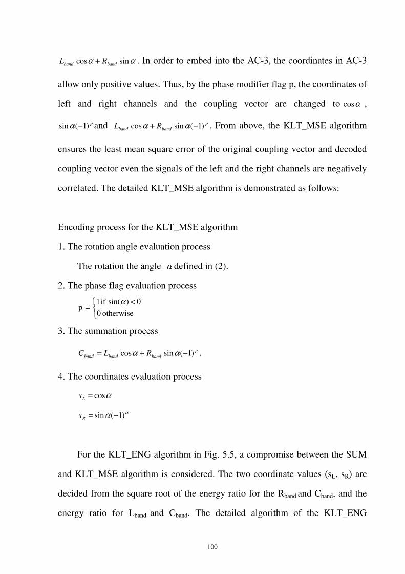
100

αα sincos bandband RL + . In order to embed into the AC-3, the coordinates in AC-3

allow only positive values. Thus, by the phase modifier flag p, the coordinates of

left and right channels and the coupling vector are changed to αcos ,

p)1(sin −α and pbandband RL )1(sincos −+ αα . From above, the KLT_MSE algorithm

ensures the least mean square error of the original coupling vector and decoded

coupling vector even the signals of the left and the right channels are negatively

correlated. The detailed KLT_MSE algorithm is demonstrated as follows:

Encoding process for the KLT_MSE algorithm

1. The rotation angle evaluation process

The rotation the angle α defined in (2).

2. The phase flag evaluation process

���

otherwise 00 < )sin( if 1

=pα

3. The summation process

pbandbandband RLC )1(sincos −+= αα .

4. The coordinates evaluation process

αcos=Ls

αα )1(sin −=Rs .

For the KLT_ENG algorithm in Fig. 5.5, a compromise between the SUM

and KLT_MSE algorithm is considered. The two coordinate values (sL, sR) are

decided from the square root of the energy ratio for the Rband and Cband, and the

energy ratio for Lband and Cband. The detailed algorithm of the KLT_ENG

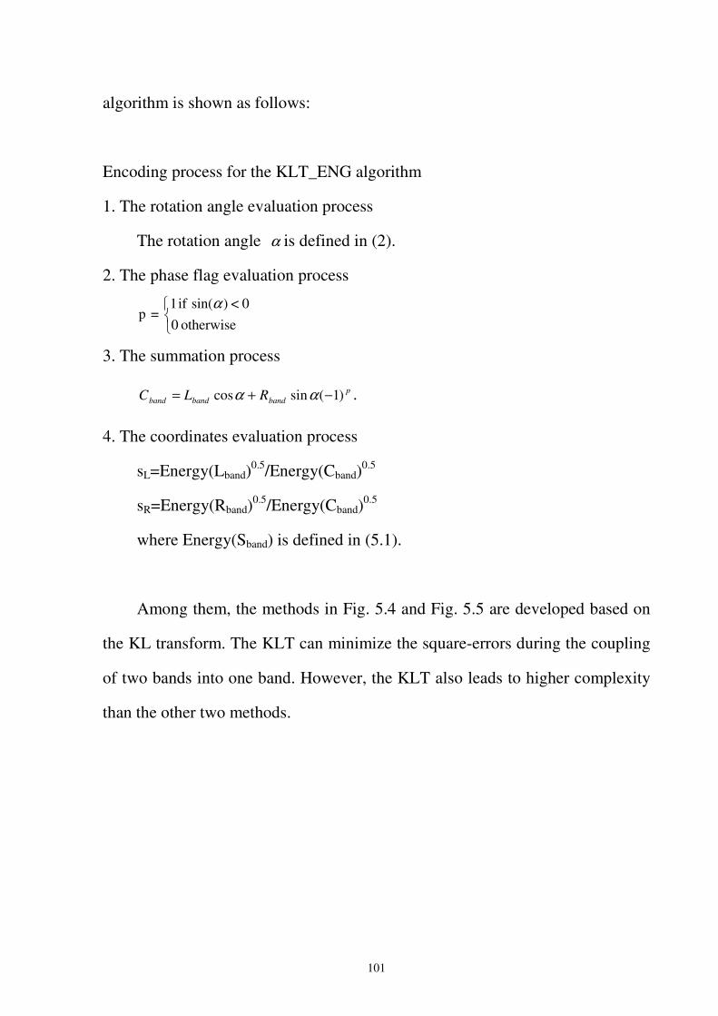
101

algorithm is shown as follows:

Encoding process for the KLT_ENG algorithm

1. The rotation angle evaluation process

The rotation angle α is defined in (2).

2. The phase flag evaluation process

���

otherwise 00 < )sin( if 1

=pα

3. The summation process

pbandbandband RLC )1(sincos −+= αα .

4. The coordinates evaluation process

sL=Energy(Lband)0.5/Energy(Cband)

0.5

sR=Energy(Rband)0.5/Energy(Cband)

0.5

where Energy(Sband) is defined in (5.1).

Among them, the methods in Fig. 5.4 and Fig. 5.5 are developed based on

the KL transform. The KLT can minimize the square-errors during the coupling

of two bands into one band. However, the KLT also leads to higher complexity

than the other two methods.

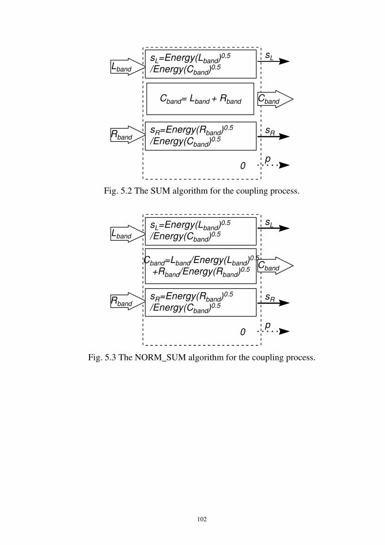
102

Cband= Lband + Rband

Lband

Rband

Cband

sL

sR

p

sL=Power(Lband)/Power(Cband)

sL=Power(Lband)/Power(Cband)

0

sL=Energy(Lband)0.5

/Energy(Cband)0.5

sR=Energy(Rband)0.5

/Energy(Cband)0.5

Fig. 5.2 The SUM algorithm for the coupling process.

Cband= Lband/Power(Lband)+ Rband /Power(Rband)

sL=Power(Lband)/Power(Cband)Lband

RbandsL=Power(Rband)

/Power(Cband)

Cband

0

sL

sR

p

sL=Energy(Lband)0.5

/Energy(Cband)0.5

sR=Energy(Rband)0.5

/Energy(Cband)0.5

Cband=Lband/Energy(Lband)0.5

+Rband/Energy(Rband)0.5

Fig. 5.3 The NORM_SUM algorithm for the coupling process.

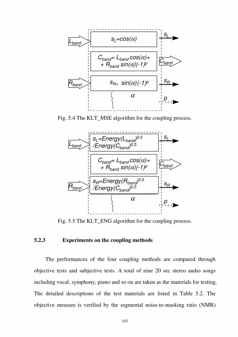
103

Cband= Lband cos(α)++ Rband sin(α)(-1)p

sL=cos(α)Lband

Rband sL= sin(α)

Cband

��

sL

sR

p

sR= (-1)p

Fig. 5.4 The KLT_MSE algorithm for the coupling process.

Cband= Lband cos(α)++ Rband sin(α)(-1)p

Lband

Rband

Cband

sL

sR

p��

sL=Power(Lband)/Power(Cband)

sL=Power(Rband)/Power(Cband)

sL=Energy(Lband)0.5

/Energy(Cband)0.5

sR=Energy(Rband)0.5

/Energy(Cband)0.5

Fig. 5.5 The KLT_ENG algorithm for the coupling process.

5.2.3 Experiments on the coupling methods

The performances of the four coupling methods are compared through

objective tests and subjective tests. A total of nine 20 sec stereo audio songs

including vocal, symphony, piano and so on are taken as the materials for testing.

The detailed descriptions of the test materials are listed in Table 5.2. The

objective measure is verified by the segmental noise-to-masking ratio (NMR)

104

value defined by averaging the NMR values in each coupling band in each

frame as

� � −=f b

bfbfseg SNRSMRBF

NMR )1

(1

,,

where the SMR stands for the signal-to-masking ratio in dB, the SNR for the

signal-to-noise ratio in dB, F for the total audio frames, f for the frame number,

B for the total coupling bands, and b for the coupling band number. Negative

values of the NMRseg indicate that the noise of the coded signal is inaudible, and

larger negative values of NMRseg indicate the noise may be more inaudible. The

coupling scheme is performed in the range of 3.14 KHz to 12.45 KHz. The

coupling methods are performed under high bit rate and the exponents are

transmitted with D15 mode for six times in a frame. Table 5.3 illustrates the

testing results. The results indicate that the KLT_MSE and KLT_ENG

algorithm can have better NMRseg values than the SUM and NORM_SUM

algorithm. The SUM and NORM_SUM algorithms cause coupling artifacts and

poor NMRseg values due to signal cancellation when Lband and Rband are

negatively correlated. We further consider the encoding for the bit rate at 128

kbits/s and the exponents strategy D15 is transmitted once per frame. The test

results are summarized in Table 5.4 that indicates the order of the performance

being the KLT_MSE, KLT_ENG, SUM and NORM_SUM algorithm.

In the subjective test under the critical bit rate at 128 kbits/s, the same test

materials in Table 5.2 are evaluated. The results of the listening test show the

order of the quality performance of the four coupling methods is the KLT_ENG,

SUM, NORM_SUM, and KLT_MSE algorithm. Although the excellent

performance of the objective tests, the KLT_MSE algorithm gives poor

105

subjective performance due to some ringing noise. The noise may be due to the

discontinuous coordinates across different bands in the KLT_MSE algorithm.

To sum up, the KLT_ENG algorithm gives high performances on both objective

and subjective tests because it takes the advantages from the KLT_MSE

algorithm on the signal preservation and the SUM algorithm on the energy

preservation.

5.2.4 Dithering on the coupling bands

In AC-3, dithering scheme is to add white noise to the coded bands in the

decoding process. For low bit rate audio coding, quantization leads to the noises

that are correlated with signals. Such a correlation is very sensitive for the

human hearing systems. Especially, the coupling scheme can also lead to the

artifacts as mentioned in last section. Dithering can reduce the artifacts from

either the quantization or the coupling process. The four coupling methods

presented in last section are examined through subjective tests when the

dithering in AC-3 is applied. In our subjective listening test for the SUM and

NORM_SUM algorithm, the dithering can significantly reduce the coupling

noise. As a result, the quality from the KLT_ENG, SUM, and NORM_SUM

algorithm become indistinguishable when the dithering is applied.

5.2.5 Remarks

In this section, four coupling methods for the AC-3 encoder have been

introduced. These four methods vary with the complexity and performance.

Both subjective and objective tests have been conducted and demonstrated the

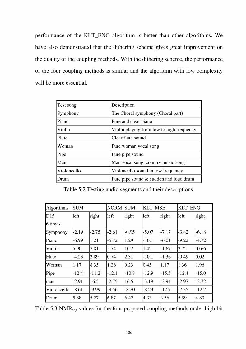
106

performance of the KLT_ENG algorithm is better than other algorithms. We

have also demonstrated that the dithering scheme gives great improvement on

the quality of the coupling methods. With the dithering scheme, the performance

of the four coupling methods is similar and the algorithm with low complexity

will be more essential.

Test song Description

Symphony The Choral symphony (Choral part)

Piano Pure and clear piano

Violin Violin playing from low to high frequency

Flute Clear flute sound

Woman Pure woman vocal song

Pipe Pure pipe sound

Man Man vocal song; country music song

Violoncello Violoncello sound in low frequency

Drum Pure pipe sound & sudden and loud drum

Table 5.2 Testing audio segments and their descriptions.

Algorithms SUM NORM_SUM KLT_MSE KLT_ENG

D15

6 times

left right left right left right left right

Symphony -2.19 -2.75 -2.61 -0.95 -5.07 -7.17 -3.82 -6.18

Piano -6.99 1.21 -5.72 1.29 -10.1 -6.01 -9.22 -4.72

Violin 5.90 7.81 5.74 10.2 1.42 -1.67 2.72 -0.66

Flute -4.23 2.89 0.74 2.31 -10.1 -1.36 -9.49 0.02

Woman 1.17 8.35 1.26 9.23 0.45 1.17 1.36 1.96

Pipe -12.4 -11.2 -12.1 -10.8 -12.9 -15.5 -12.4 -15.0

man -2.91 16.5 -2.75 16.5 -3.19 -3.94 -2.97 -3.72

Violoncello -8.61 -9.99 -9.56 -8.20 -8.23 -12.7 -7.35 -12.2

Drum 5.88 5.27 6.87 6.42 4.33 3.56 5.59 4.80

Table 5.3 NMRseg values for the four proposed coupling methods under high bit

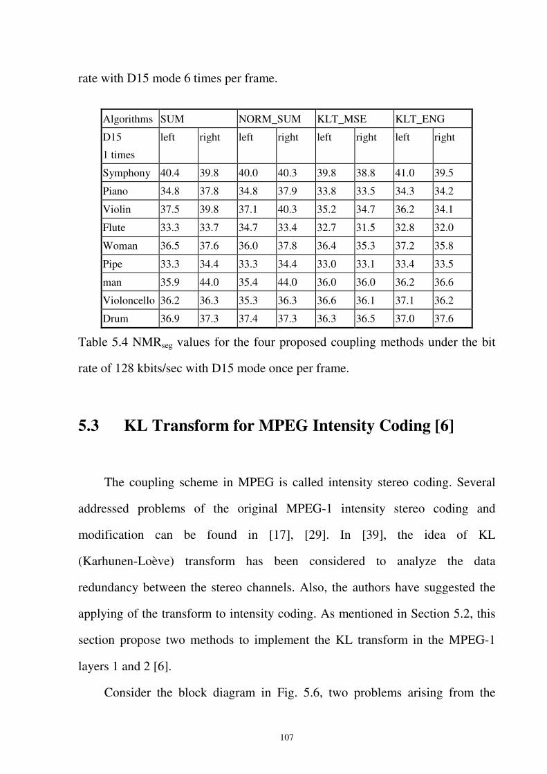
107

rate with D15 mode 6 times per frame.

Algorithms SUM NORM_SUM KLT_MSE KLT_ENG

D15

1 times

left right left right left right left right

Symphony 40.4 39.8 40.0 40.3 39.8 38.8 41.0 39.5

Piano 34.8 37.8 34.8 37.9 33.8 33.5 34.3 34.2

Violin 37.5 39.8 37.1 40.3 35.2 34.7 36.2 34.1

Flute 33.3 33.7 34.7 33.4 32.7 31.5 32.8 32.0

Woman 36.5 37.6 36.0 37.8 36.4 35.3 37.2 35.8

Pipe 33.3 34.4 33.3 34.4 33.0 33.1 33.4 33.5

man 35.9 44.0 35.4 44.0 36.0 36.0 36.2 36.6

Violoncello 36.2 36.3 35.3 36.3 36.6 36.1 37.1 36.2

Drum 36.9 37.3 37.4 37.3 36.3 36.5 37.0 37.6

Table 5.4 NMRseg values for the four proposed coupling methods under the bit

rate of 128 kbits/sec with D15 mode once per frame.

5.3 KL Transform for MPEG Intensity Coding [6]

The coupling scheme in MPEG is called intensity stereo coding. Several

addressed problems of the original MPEG-1 intensity stereo coding and

modification can be found in [17], [29]. In [39], the idea of KL

(Karhunen-Loève) transform has been considered to analyze the data

redundancy between the stereo channels. Also, the authors have suggested the

applying of the transform to intensity coding. As mentioned in Section 5.2, this

section propose two methods to implement the KL transform in the MPEG-1

layers 1 and 2 [6].

Consider the block diagram in Fig. 5.6, two problems arising from the

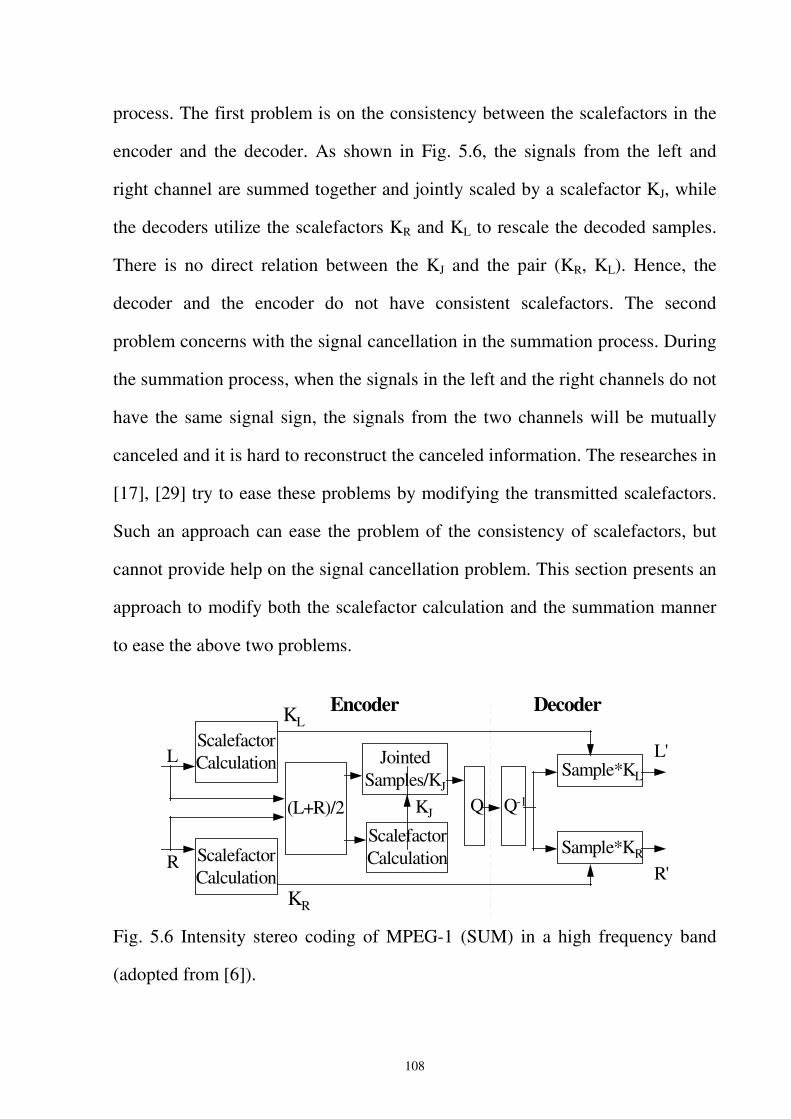
108

process. The first problem is on the consistency between the scalefactors in the

encoder and the decoder. As shown in Fig. 5.6, the signals from the left and

right channel are summed together and jointly scaled by a scalefactor KJ, while

the decoders utilize the scalefactors KR and KL to rescale the decoded samples.

There is no direct relation between the KJ and the pair (KR, KL). Hence, the

decoder and the encoder do not have consistent scalefactors. The second

problem concerns with the signal cancellation in the summation process. During

the summation process, when the signals in the left and the right channels do not

have the same signal sign, the signals from the two channels will be mutually

canceled and it is hard to reconstruct the canceled information. The researches in

[17], [29] try to ease these problems by modifying the transmitted scalefactors.

Such an approach can ease the problem of the consistency of scalefactors, but

cannot provide help on the signal cancellation problem. This section presents an

approach to modify both the scalefactor calculation and the summation manner

to ease the above two problems.

ScalefactorCalculation

ScalefactorCalculation

(L+R)/2

L

R

JointedSamples/KJ

ScalefactorCalculation

KJ Q Q-1

Sample*KL

Sample*KR

L'

R'

KL

KR

Encoder Decoder

Fig. 5.6 Intensity stereo coding of MPEG-1 (SUM) in a high frequency band

(adopted from [6]).

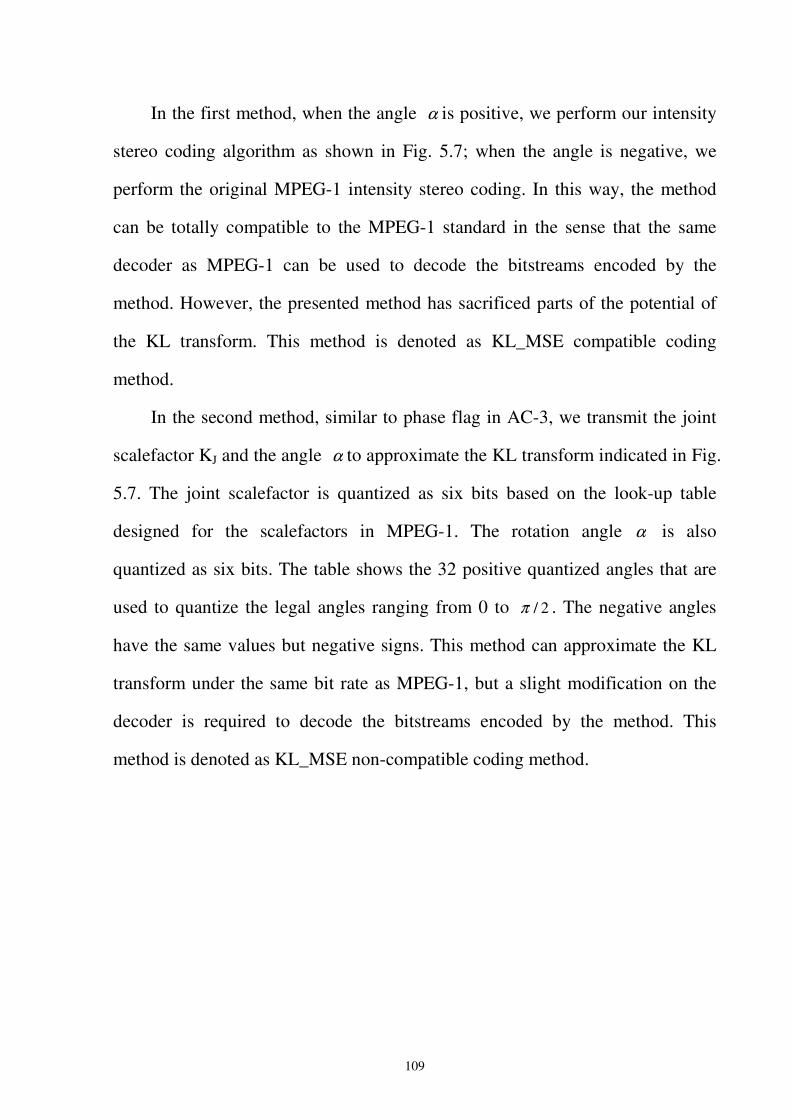
109

In the first method, when the angle α is positive, we perform our intensity

stereo coding algorithm as shown in Fig. 5.7; when the angle is negative, we

perform the original MPEG-1 intensity stereo coding. In this way, the method

can be totally compatible to the MPEG-1 standard in the sense that the same

decoder as MPEG-1 can be used to decode the bitstreams encoded by the

method. However, the presented method has sacrificed parts of the potential of

the KL transform. This method is denoted as KL_MSE compatible coding

method.

In the second method, similar to phase flag in AC-3, we transmit the joint

scalefactor KJ and the angle α to approximate the KL transform indicated in Fig.

5.7. The joint scalefactor is quantized as six bits based on the look-up table

designed for the scalefactors in MPEG-1. The rotation angle α is also

quantized as six bits. The table shows the 32 positive quantized angles that are

used to quantize the legal angles ranging from 0 to 2/π . The negative angles

have the same values but negative signs. This method can approximate the KL

transform under the same bit rate as MPEG-1, but a slight modification on the

decoder is required to decode the bitstreams encoded by the method. This

method is denoted as KL_MSE non-compatible coding method.

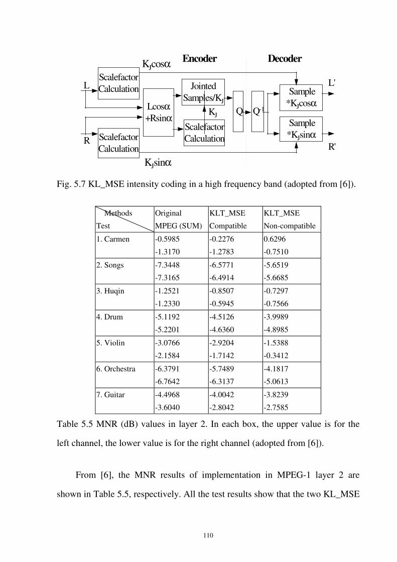
110

ScalefactorCalculation

ScalefactorCalculation

Lcosα+Rsinα

L

R

JointedSamples/KJ

ScalefactorCalculation

KJ Q Q-1

Sample*KJcosα

Sample*KJsinα

L'

R'

KJcosα Encoder Decoder

KJsinα

Fig. 5.7 KL_MSE intensity coding in a high frequency band (adopted from [6]).

Methods

Test

Original

MPEG (SUM)

KLT_MSE

Compatible

KLT_MSE

Non-compatible

1. Carmen -0.5985

-1.3170

-0.2276

-1.2783

0.6296

-0.7510

2. Songs -7.3448

-7.3165

-6.5771

-6.4914

-5.6519

-5.6685

3. Huqin -1.2521

-1.2330

-0.8507

-0.5945

-0.7297

-0.7566

4. Drum -5.1192

-5.2201

-4.5126

-4.6360

-3.9989

-4.8985

5. Violin -3.0766

-2.1584

-2.9204

-1.7142

-1.5388

-0.3412

6. Orchestra -6.3791

-6.7642

-5.7489

-6.3137

-4.1817

-5.0613

7. Guitar -4.4968

-3.6040

-4.0042

-2.8042

-3.8239

-2.7585

Table 5.5 MNR (dB) values in layer 2. In each box, the upper value is for the

left channel, the lower value is for the right channel (adopted from [6]).

From [6], the MNR results of implementation in MPEG-1 layer 2 are

shown in Table 5.5, respectively. All the test results show that the two KL_MSE

111

intensity coding methods can have a lower MNRs than the original MPEG

intensity coding method. Among the two KL intensity coding methods, the

KL_MSE non-compatible coding method can have a better performance than the

compatible one.

5.4 Concluding Remarks

KL transform is introduced to obtained the optimal solution for the

coupling process in numerical sense. When integrating the KL transform into

coupling schemes of MPEG and AC-3, two issues arise. The first issue lies on

KL coupling scheme might not perceptually optimal even if it is optimal in

numerical sense. Second, due to the constraints of different audio coders, KL

coupling scheme might not tightly integrate with stereo matrix design of

different coders. For example, in MPEG, during the summation process, when

the signals in the left and right channels do not have the same signal sign, the

signals from the two channels will be mutually canceled and it is hard to

reconstruct the canceled information.

112

Chapter 6 Conclusions and Future Works

6.1 Concluding Remarks

This dissertation has studied the design of audio standards: MPEG-1/2 and

AC-3. We have proposed the fast algorithms for the filterbank, the

psychoacoustic model, and the bit allocation. Also, this dissertation has designed

the new intensity/coupling schemes.

On the filterbank, a unified fast algorithm of filterbank for variant form and

variant size has been presented. On the psychoacoustic model, a hybrid

filterbank has been proposed to replace to original frequency analyzer, Fourier

transform. On the bit allocation, we first present the efficient bit allocation

method for MPEG layer 3 with non-uniform quantization and variable length

coding and then present criteria for the bit allocation for Dolby AC-3 and

propose efficient bit allocation algorithm according to the criteria. On the

intensity/coupling, this dissertation applied KL transform to design the

parameters for MPEG and AC-3 to have a better encoding quality.

113

6.2 Future Works

This dissertation studies the design issues and experiments based on the

MPEG-1 and AC-3. However, the design concepts are never restricted to the

two standards. The applying of the design concepts under the constraints of the

protocols by new standards such as MPEG AAC and MPEG4 is the direct

extension of the dissertation. In Chapter 2: unified algorithm for fast filterbank

computing, this dissertation proposes fast algorithms that unify the variant form

and variant size of cosine modulated filter banks. The size of the cosine

modulated filter banks is limited to a number of power of 2 due to the recursion

of the fast algorithm. In fact, in MPEG-1 and MPEG-4, there are exceptions for

this constraint. More researches for this issue can be studied. In Chapter 4: fast

bit allocation method, this dissertation proposes an efficient bit allocation

algorithm for mono channel of MPEG layer 3. More researches can be studied

on the efficient bit allocation algorithms of variable bit rate for each frame and

efficient algorithms for stereo channels. MPEG allows variable bit rate for each

frame. This gives more flexibility to ensure perceptual quality according to the

information from psychoacoustic model. When a frame deserves more bits

according to psychoacoustic model, more bit rate will be given iteratively or

predictive until ensuring quality. When a frame deserves fewer bits, fewer bits

will be given iteratively or predictive. For stereo channels, MPEG layer 3 allows

bit numbers can be shared in variant ratio for left/right or middle/side channel by

the mechanism of bit reservoir and joint stereo coding. For the more and more

complexity of the variable bit rate and bit share ratio for stereo channel, the

114

proposed algorithm mentioned in section 4.2 provides more potential for

efficient bit allocation.

New mechanisms such as gain control, temporal noise shaping, prediction,

and transform domain interleaved vector quantization give more potential for

quality improvement, but these modules also lead to new design issues on

combining with the design modules discussed in this dissertation. The combined

consideration with these modules is another issue deserving further study.

115

Bibliography

[1] B. Edler, “Aliasing reduction in sub-bands of cascaded filterbanks with decimation,” Electronic Letters, vol. 28, no. 12, pp. 1104-1106, Jun. 1992.

[2] B. G. Lee, “A new algorithm for computing the discrete cosine transform,” IEEE Transaction Acoustic, Speech, Signal Processing, vol. ASSP-32, pp. 1243-1245, Dec. 1984.

[3] C. C. Todd, G. A. Davidson, M. D. Davis, L. D. Fielder, B. D. Link, S. Vernon, “AC-3: flexible perceptual coding for audio transmission and storage,” AES 96th Conversion, Feb. 1994.

[4] C.M. Liu, C.C. Chen, W. C. Lee, and S.W. Lee, “A fast bit allocation method for MPEG layer III,” Int. Conf. on Consumer Electronics, pp. 22 –23, 1999.

[5] C. M. Liu and C.W. Jen, “On the design of VLSI arrays for discrete Fourier transform,” IEE Proceedings-G, vol. 139, no. 4, pp. 541-552, Aug. 1992.

[6] C. M. Liu and J. C. Liu, “A new intensity stereo coding scheme for MPEG audio encoder- layer I and II,” IEEE Transaction on Consumer Electronics, vol. 42, pp. 535-539, Aug. 1996.

[7] C. M. Liu and J. C. Liu, “A new intensity stereo coding scheme for MPEG1 audio encoder- layer I and II,” IEEE Transactions on Consumer Electronics, vol. 42, pp. 535-539, Aug. 1996.

[8] C. M. Liu, S. W. Lee, and W. C. Lee, “Bit allocation method for AC-3 encoder,” IEEE Transactions on Consumer Electronics, vol. 44 Issue: 3, pp. 883 –887, Aug. 1998

[9] C. M. Liu, S. W. Lee, and W. C. Lee, “Bit allocation method for Dolby AC-3 encoder ,” Int. Conf. on Consumer Electronics, pp. 330 –331, 1998.

116

[10] C. M. Liu, W. C. Lee, “The design of a hybrid filterbank for the psychoacoustic model in ISO/MPEG phases 1, 2 audio encoder ,” IEEE Transactions on Consumer Electronics, vol. 43 issue: 3, pp. 586 –592, Aug. 1997.

[11] C. M. Liu, W. C. Lee, S. Y. Juang, “Design of the coupling schemes for the AC-3 coder in stereo coding,” IEEE Transactions on Consumer Electronics, vol. 44 issue: 3 , pp. 878 –882, Aug. 1998.

[12] C. M. Liu, W. C. Lee, "A unified fast algorithm for cosine-modulated filterbanks in current audio standards," Journal of AES, vol. 47, no. 12, Dec 1999.

[13] C. M. Liu, W. C. Lee, “The design of a hybrid filterbank for the psychoacoustic model in ISO/MPEG phase 1, 2 audio encoder,” Int. Conf. on Consumer Electronics, pp. 208 –209, 1997.

[14] C. M. Liu, W. C. Lee, S. Y. Juang, “Design of the coupling schemes for the Dolby AC-3 coder in stereo coding,” Int. Conf. on Consumer Electronics, pp. 328 –329, 1998.

[15] C. M. Liu, W. C. Lee, "A unified fast algorithm for cosine-modulated filterbanks in current audio standards," 104th AES Convention, 1998.

[16] C. W. Kok, “Fast algorithm for computing discrete cosine transform,” IEEE Transaction on Signal Processing, vol. 45, no. 3, pp. 757-760, Mar. 1997.

[17] D. H. Teh, A. P. Tan, “An improved stereophonic coding scheme compatible to the ISO/MPEG audio coding algorithm,” ICCS, pp. 437-441, 1992.

[18] D. H. Teh, S. N. Koh, and A. P. Tan, “Efficient bit allocation algorithm for ISO/MPEG audio encoder,” IEEE electronics letter, vol. 34, no. 8, Apr 16th, 1988.

[19] E. O. Brigham, “The fast Fourier transform and its application,” Prentice Hall Inc., 1988.

[20] H. D. Yun and S. U. Lee, “On the fixed-point-error analysis of several fast DCT algorithms,” IEEE Transaction Circuits System Video Technology, vol. 3, pp. 27-41, Feb. 1991.

117

[21] G. A. Dividson, L. D. Fielder, B. D. Link, “Parameter bit allocation in a perceptual audio coder,” AES 97th Conversion, Nov. 1994.

[22] H.T. Kung, “Special purpose devices for signal and image processing: an opportunity in very large scale integration (VLSI),” Proceedings of SPIE, (Real Time Signal Processing III), 241, pp. 76-84, 1980.

[23] ISO/IEC 13818-3, “Information technology -generic coding of moving pictures and associated audio: audio,” ISO/IEC JTC1/SC29/WG11 NO803, Nov. 1994.

[24] ISO/IEC JTCI/SC29, “Information technology- coding of moving pictures and associated audio for digital storage media at up to 1.5 mps- CD11172 (part 3, audio),” Doc. ISO/IEC JTCI/SC29 NO71.

[25] ISO/IEC JTC1/SC29/WG11, “Coding of moving pictures and audio- IS 13818-7 (MPEG-2 Advanced Audio Coding, AAC),” Doc. ISO/IEC JTC1/SC29/WG11 n1650, Apr. 1997.

[26] J. B. Allen, “Speech and hearing in communication,” The Acoustical Society of America by the American Institute of Physics.

[27] J. C. McKinney, R. Hopkins, “Digital audio compression standard (AC-3),” Advanced television system committee, Dec. 1995.

[28] J. D. Johnston, “Transform coding of audio signals using perceptual noise criteria,” IEEE Journal on Selected Area in Communications, vol. 6, no. 2, pp. 314-323, Feb. 1988.

[29] J. Herre, K. Brandenburg, D. Lederer, “Intensity stereo coding,” 96th AES Convention, Feb. 1994.

[30] J. P. Prince and A. W. Johnson, A. B. Bradley, “Subband/transform coding using filterbank design based on time domain aliasing cancellation,” Proc. Int. Conf. Acoustic, Speech, Signal Processing, pp. 2161-2164, 1987.

[31] K. Brandenburg, “MP3 and AAC explained,” AES 17th Int. Conf. on High Quality Audio Coding.

[32] K. Brandenburg, E. Eberlein, J. Herre, B. Edler, “Comparison of filterbanks for high quality audio coding,” IEEE Int. Symposium on Circuit and Systems, vol. 3, pp. 1336-1339, 1992.

118

[33] K. Brandenburg, J. D. Johnston, “Second level perceptual audio coding: the hybrid coder,” 88th Convention of AES, March 13-16, 1990.

[34] K. R. Rao and P. Yip, “Discrete cosine transform- algorithm, advantages, application,” Academic press. Inc., 1990.

[35] K. T. Fung, Y. L. Chan and W. C. Siu, “A fast bit allocation algorithm for MPEG audio encoder,” Proc. of 2001 Int. symposium on Intelligent Multimedia, Video and Speech Processing, May 2001.

[36] N. S. Jayant, Peter Noll, “Digital coding of waveforms principles and applications to speech and video,” Prentice-hall Inc.

[37] P. Yip and K. R. Rao, “Fast decimation-in-time algorithms for a family of discrete sin and cosine transforms,” Circuit System, Signal Processing, pp. 387-408, vol. 3, 1984.

[38] P. P. Vaidyanthan, “Multirate digital filters,” Prentice Hall Inc., 1993.

[39] R. G. V. D. Waal and R. N. J. Veldhuis, "Subband coding of stereophonic digital audio signals," ICASSP, pp. 3601-3604, 1991.

[40] R N. J. Veldhuis, "Bit rates in audio source coding," IEEE Journal on Selected Areas in Communications, vol. 10, no. 1, pp. 86-96, Jan. 1992.

[41] S. Shlien, “The modulated lapped transform, its time-varying forms, and its application to audio coding standards,” IEEE Transaction on Speech and Audio Processing, vol. 5, no. 4, pp. 359-366, July 1997.

[42] T. Sporer, K. Brandenburg, B. Edler, “The use of multirate filterbanks for coding of high quality digital audio,” The 6th European Signal Processing Conf., vol. 1, pp. 211-214, Jun. 1992.

[43] “United States advanced television systems committee digital audio compression (AC-3) ATSC standard,” Dolby Labs, A52.doc, 1994.

[44] X. Wei, M. J. Shaw, M. R. Varley, “Optimum bit allocation and decomposition for high quality audio coding,” Proc. Int. Conf. Acoustic, Speech, Signal Processing, vol. 1, pp. 315-318, 1997.

119

[45] Z. Cvetkovic and M. V. Popvic, “New fast recursive algorithms for the computation of discrete cosine transform,” IEEE Transaction on Signal Processing, vol. 40, pp. 2083-2086, Aug. 1992.

120

Curriculum Vita

Wen-Chieh Lee was born in Toayuan, Taiwan in Oct. 1972. He received the B.

S. degree from the Department of Computer Science and Information

Engineering, National Chiao Tung University, Hsinchu, Taiwan in 1995. He is

currently a Ph. D. candidate of the Department of Computer Science and

Information Engineering, National Chiao Tung University, Hsinchu, Taiwan.

His research interests are audio compression and real-time computer

architecture.

121

Publication Lists

Journal Papers:

[1] C. M. Liu, W. C. Lee, “The design of a hybrid filterbank for the psychoacoustic model in ISO/MPEG phases 1, 2 audio encoder,” IEEE Transactions on Consumer Electronics, vol. 43 issue: 3, pp. 586 –592, Aug. 1997.

[2] C. M. Liu, W. C. Lee, S. Y. Juang, “Design of the coupling schemes for the AC-3 coder in stereo coding,” IEEE Transactions on Consumer Electronics, vol. 44 issue: 3, pp. 878 –882, Aug. 1998.

[3] C. M. Liu, S. W. Lee, and W. C. Lee, “Bit allocation method for AC-3 encoder,” IEEE Transactions on Consumer Electronics, vol. 44 issue: 3, pp. 883 –887, Aug. 1998.

[4] C. M. Liu, W. C. Lee, "A unified fast algorithm for cosine modulated filterbanks in current audio standards," Journal of Audio Engineering Society, vol. 47, no. 12, Dec 1999.

US Patents:

[5] C. M. Liu, W. C. Lee, “Unified recursive decomposition architecture for cosine modulated filterbanks,” U.S. Patent US6119080, Sept. 12, 2000 / June 17, 1998.

ROC Patents:

[6] C. M. Liu, W. C. Lee, “ ,”TW patent 087112476.

Conference Papers:

122

[7] C. M. Liu, W. C. Lee, “The design of a hybrid filterbank for the psychoacoustic model in ISO/MPEG phase 1, 2 audio encoder,” Int. Conf. on Consumer Electronics, pp. 208 –209, 1997.

[8] C. M. Liu, W. C. Lee, S. Y. Juang, “Design of the coupling schemes for the Dolby AC-3 coder in stereo coding,” Int. Conf. on Consumer Electronics, pp. 328 –329, 1998.

[9] C. M. Liu, W. C. Lee, “A unified fast algorithm for cosine modulated filterbanks in current audio standards,” 104th AES convention, 1998.

[10] C. M. Liu, S. W. Lee, and W. C. Lee, “Bit allocation method for Dolby AC-3 encoder ,” Int. Conf. on Consumer Electronics, pp. 330 –331, 1998.

[11] C.M. Liu, C.C. Chen, W. C. Lee, and S.W. Lee, “A fast bit allocation method for MPEG layer III,” Int. Conf. on Consumer Electronics, pp. 22 –23, 1999.