Digital Audio Coding – Dr. T. Collins Standard MIDI Files Perceptual Audio Coding MPEG-1 layers 1, 2 & 3 MPEG-4

Digital Audio Coding – Dr. T. Collins Standard MIDI Files Perceptual Audio Coding MPEG-1 layers 1, 2 & 3 MPEG-4.
Dec 16, 2015
Welcome message from author
This document is posted to help you gain knowledge. Please leave a comment to let me know what you think about it! Share it to your friends and learn new things together.
Transcript
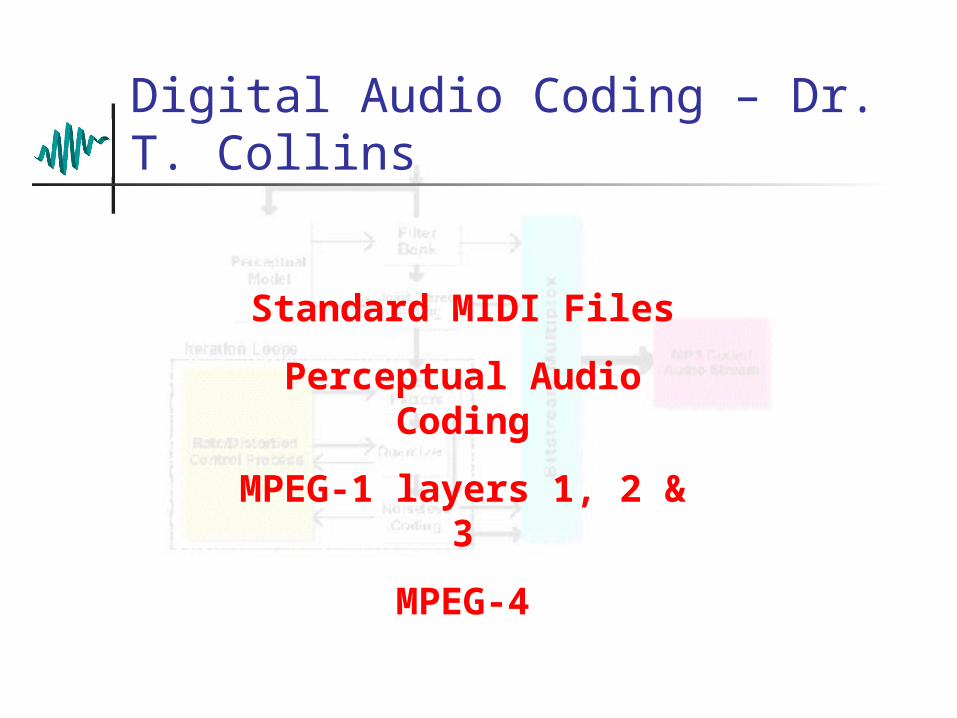
Digital Audio Coding – Dr. T. Collins
Standard MIDI Files
Perceptual Audio Coding
MPEG-1 layers 1, 2 & 3
MPEG-4
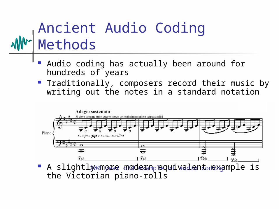
Audio coding has actually been around for hundreds of years
Traditionally, composers record their music by writing out the notes in a standard notation
A slightly more modern equivalent example is the Victorian piano-rolls
Ancient Audio Coding Methods
200 year old example of audio coding
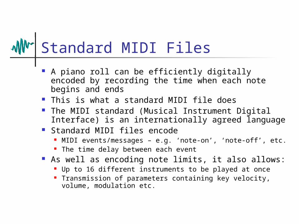
Standard MIDI Files A piano roll can be efficiently digitally encoded by
recording the time when each note begins and ends This is what a standard MIDI file does The MIDI standard (Musical Instrument Digital
Interface) is an internationally agreed language Standard MIDI files encode
MIDI events/messages – e.g. ‘note-on’, ‘note-off’, etc. The time delay between each event
As well as encoding note limits, it also allows: Up to 16 different instruments to be played at once Transmission of parameters containing key velocity,
volume, modulation etc.
Standard MIDI Limitations
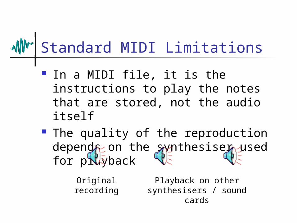
In a MIDI file, it is the instructions to play the notes that are stored, not the audio itself
The quality of the reproduction depends on the synthesiser used for playback
Original recording
Playback on other synthesisers / sound
cards
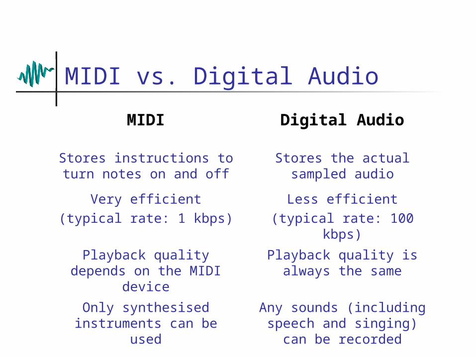
MIDI vs. Digital Audio
MIDI Digital Audio
Stores instructions to turn notes on and off
Stores the actual sampled audio
Very efficient(typical rate: 1 kbps)
Less efficient(typical rate: 100 kbps)
Playback quality depends on the MIDI device
Playback quality is always the same
Only synthesised instruments can be used
Any sounds (including speech and singing) can
be recorded
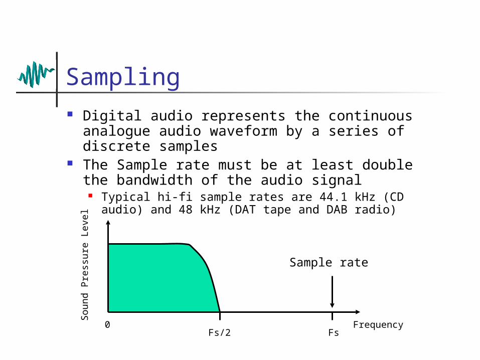
Sampling Digital audio represents the continuous
analogue audio waveform by a series of discrete samples
The Sample rate must be at least double the bandwidth of the audio signal
Typical hi-fi sample rates are 44.1 kHz (CD audio) and 48 kHz (DAT tape and DAB radio)
Soun
d P
ress
ure
Level
0Fs/2 Fs
Sample rate
Frequency
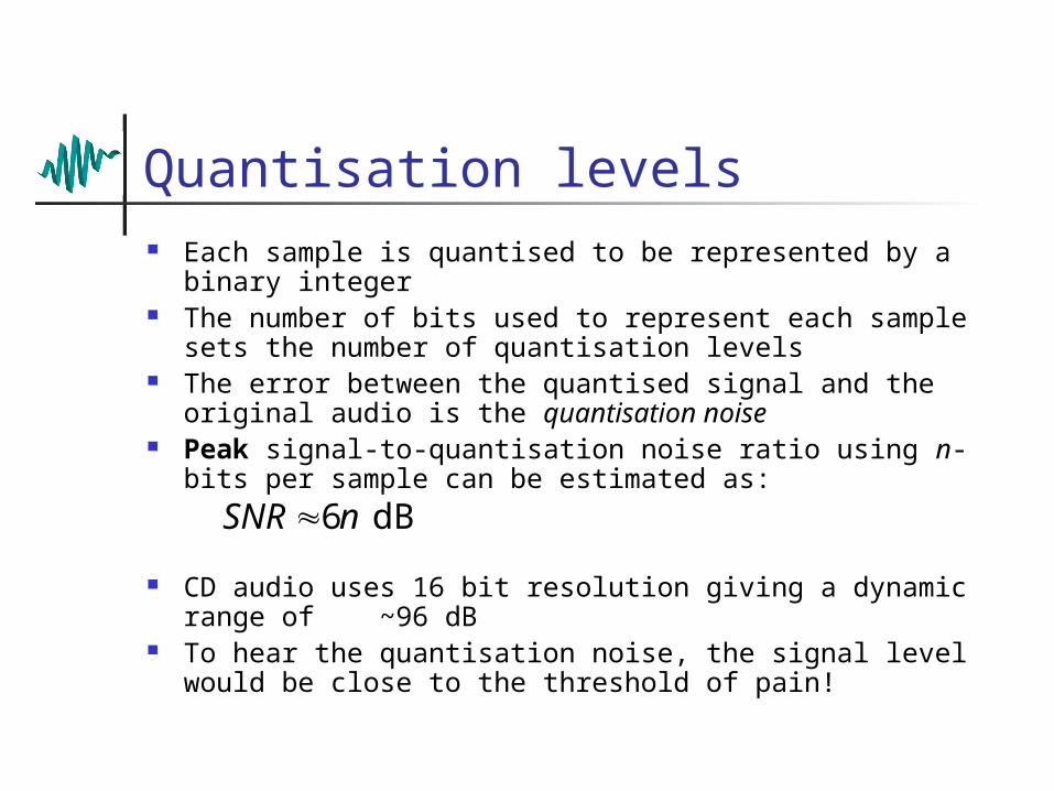
Quantisation levels Each sample is quantised to be represented by a binary
integer The number of bits used to represent each sample sets
the number of quantisation levels The error between the quantised signal and the original
audio is the quantisation noise Peak signal-to-quantisation noise ratio using n-bits per
sample can be estimated as:
CD audio uses 16 bit resolution giving a dynamic range of ~96 dB
To hear the quantisation noise, the signal level would be close to the threshold of pain!
dB 6nSNR
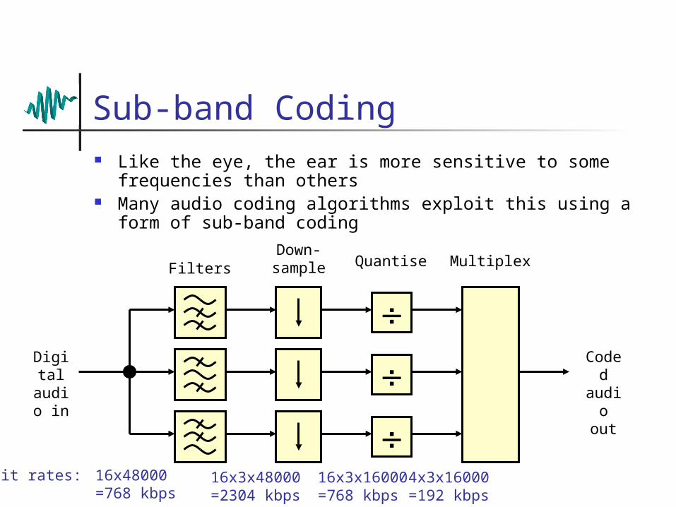
Sub-band Coding Like the eye, the ear is more sensitive to some
frequencies than others Many audio coding algorithms exploit this using a form of
sub-band codingDown-sampl
eFilters
Digital
audio in
Quantise
Coded
audio out
Multiplex
Bit rates: 16x48000=768 kbps
16x3x48000=2304 kbps
16x3x16000=768 kbps
4x3x16000=192 kbps
Perceptual Coding A key question when designing a sub-band coder:
What should the quantisation levels of the sub-bands be? Remember that the quantisation process will
introduce noise and that we want the noise to be imperceptible
We want the noise to be just below the threshold of hearing (also known as the Minimum Audible Field, MAF)
So, the question should be: What is the MAF in each sub-band?
To estimate this, look at Robinson-Dadson curves…
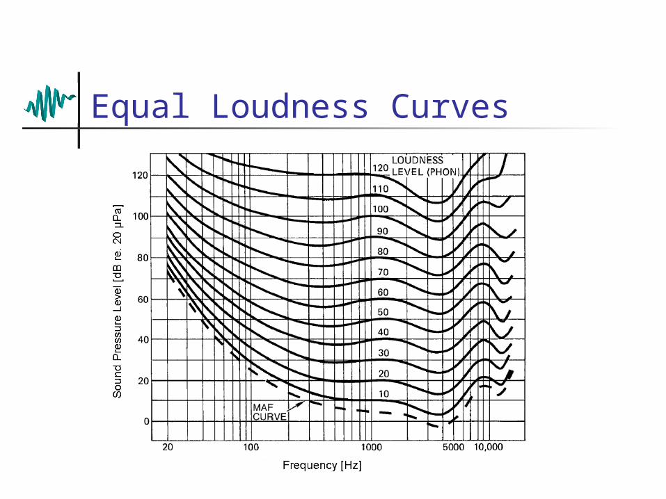
Equal Loudness Curves
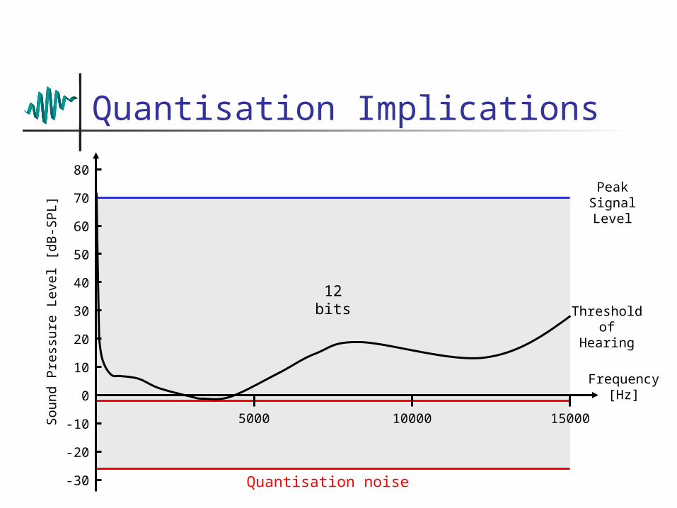
16bits
Quantisation noise
12bits
Quantisation Implications
Soun
d P
ress
ure
Level [d
B-S
PL]
80
70
60
50
40
30
20
10
0
-10
-20
-30
5000 10000 15000
Frequency [Hz]
Peak Signal Level
Threshold of Hearing
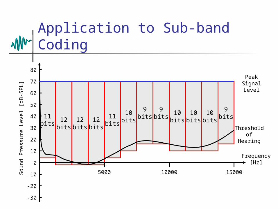
9bits
9bits
10bits
10bits
10bits
9bits
10bits
11bits
12bits
11bits
12bits
12bits
Application to Sub-band Coding
Soun
d P
ress
ure
Level [d
B-S
PL]
80
70
60
50
40
30
20
10
0
-10
-20
-30
5000 10000 15000
Frequency [Hz]
Peak Signal Level
Threshold of Hearing
Psychoacoustics
Substantial improvements to our sub-band coder are possible using psychoacoustics
Psychoacoustics is the study of how sound is perceived by the ear-brain combination
Of interest to us: how the threshold of hearing is not constant
In fact, the threshold of hearing constantly changes due to masking…
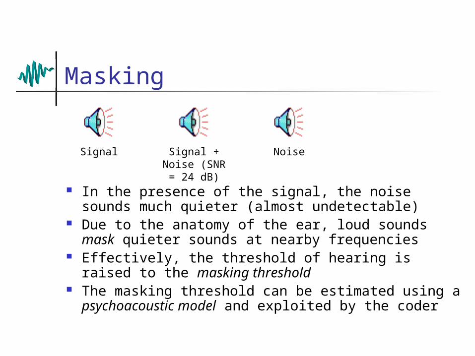
Masking
In the presence of the signal, the noise sounds much quieter (almost undetectable)
Due to the anatomy of the ear, loud sounds mask quieter sounds at nearby frequencies
Effectively, the threshold of hearing is raised to the masking threshold
The masking threshold can be estimated using a psychoacoustic model and exploited by the coder
Signal Signal + Noise (SNR = 24 dB)
Noise
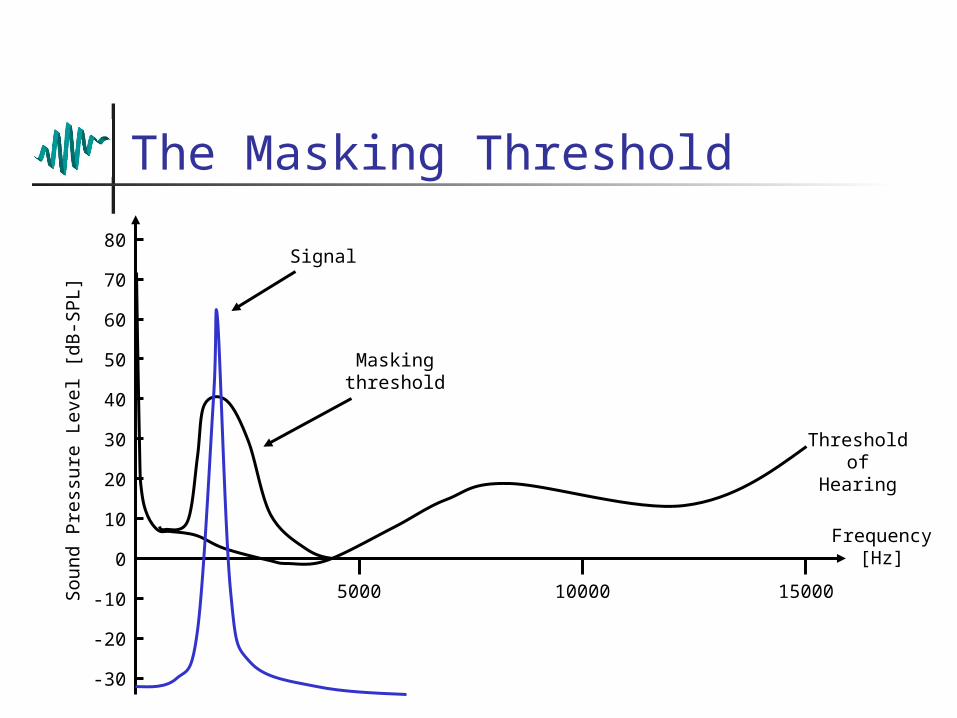
The Masking Threshold
Soun
d P
ress
ure
Level [d
B-S
PL]
80
70
60
50
40
30
20
10
0
-10
-20
-30
5000 10000 15000
Frequency [Hz]
Threshold of Hearing
Masking threshold
Signal
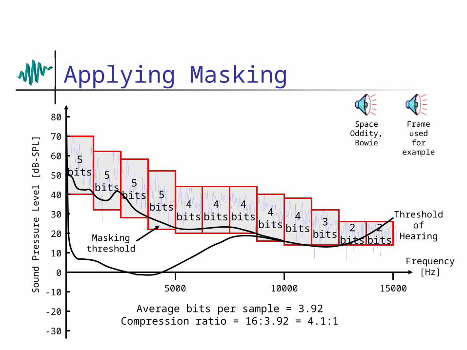
2bits
4bits
4bits 4
bits3
bits2
bits
4bits
4bits
5bits
5bits
5bits 5
bits
Applying Masking
Soun
d P
ress
ure
Level [d
B-S
PL]
80
70
60
50
40
30
20
10
0
-10
-20
-30
5000 10000 15000
Frequency [Hz]
Threshold of Hearing
Average bits per sample = 3.92Compression ratio = 16:3.92 = 4.1:1
Masking threshold
Space Oddity, Bowie
Frame used for exampl
e
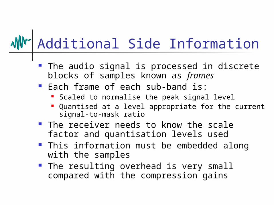
Additional Side Information The audio signal is processed in discrete blocks
of samples known as frames Each frame of each sub-band is:
Scaled to normalise the peak signal level Quantised at a level appropriate for the current signal-
to-mask ratio The receiver needs to know the scale factor and
quantisation levels used This information must be embedded along with
the samples The resulting overhead is very small compared
with the compression gains
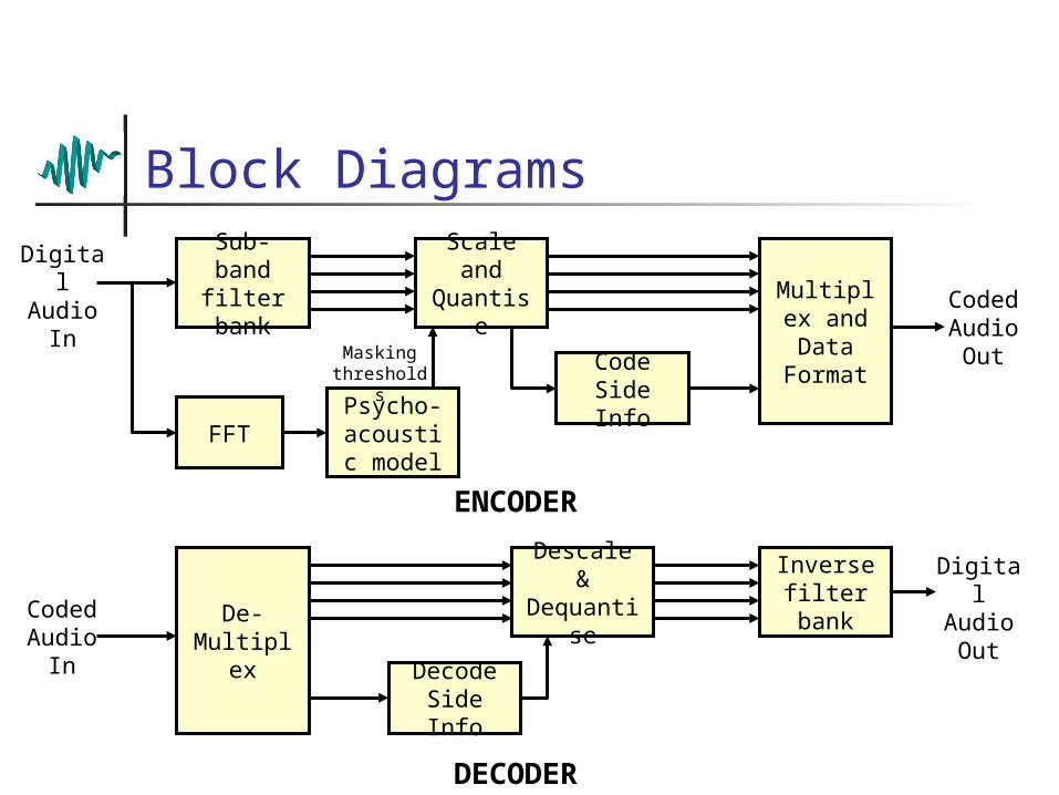
Block DiagramsSub-band filter bank
Scale and
Quantise Multiplex and Data Format
Code Side Info
FFTPsycho-acoustic model
ENCODER
Digital Audio
In
De-Multiplex
Descale & Dequantis
e
Inverse filter bank
Decode Side Info
DECODER
Digital Audio OutCoded
Audio In
Coded Audio OutMasking
thresholds
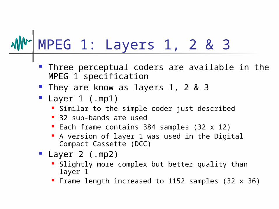
MPEG 1: Layers 1, 2 & 3 Three perceptual coders are available in the
MPEG 1 specification They are know as layers 1, 2 & 3 Layer 1 (.mp1)
Similar to the simple coder just described 32 sub-bands are used Each frame contains 384 samples (32 x 12) A version of layer 1 was used in the Digital Compact
Cassette (DCC) Layer 2 (.mp2)
Slightly more complex but better quality than layer 1 Frame length increased to 1152 samples (32 x 36)
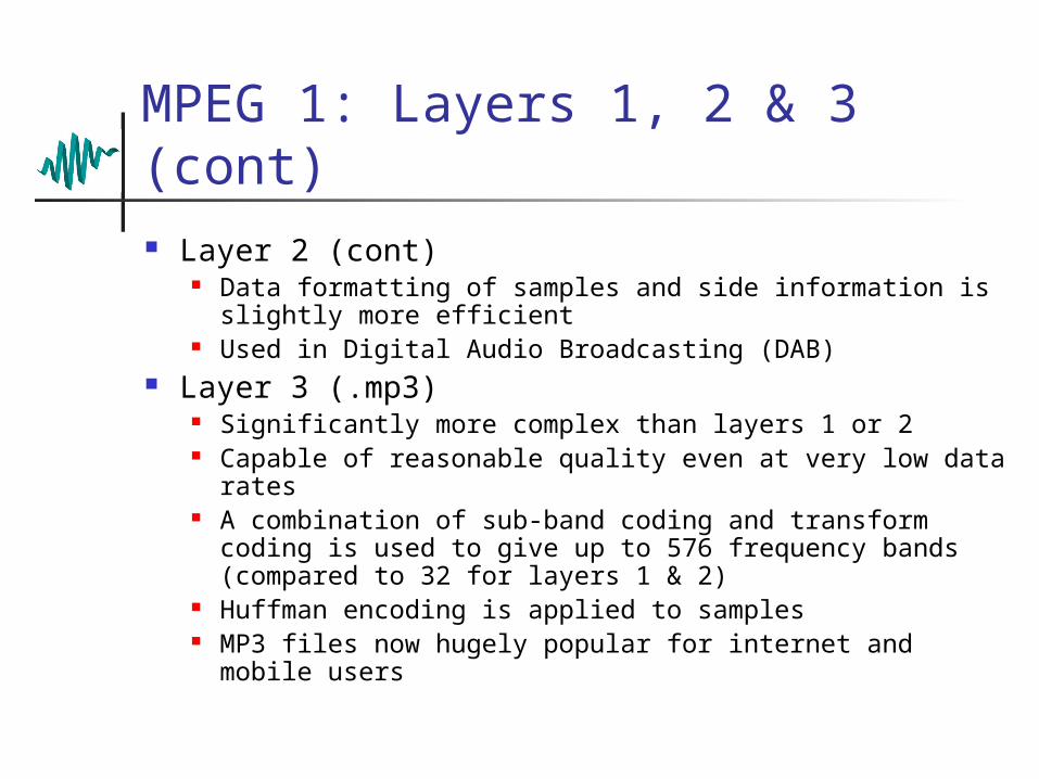
MPEG 1: Layers 1, 2 & 3 (cont) Layer 2 (cont)
Data formatting of samples and side information is slightly more efficient
Used in Digital Audio Broadcasting (DAB) Layer 3 (.mp3)
Significantly more complex than layers 1 or 2 Capable of reasonable quality even at very low data rates A combination of sub-band coding and transform coding is
used to give up to 576 frequency bands (compared to 32 for layers 1 & 2)
Huffman encoding is applied to samples MP3 files now hugely popular for internet and mobile
users
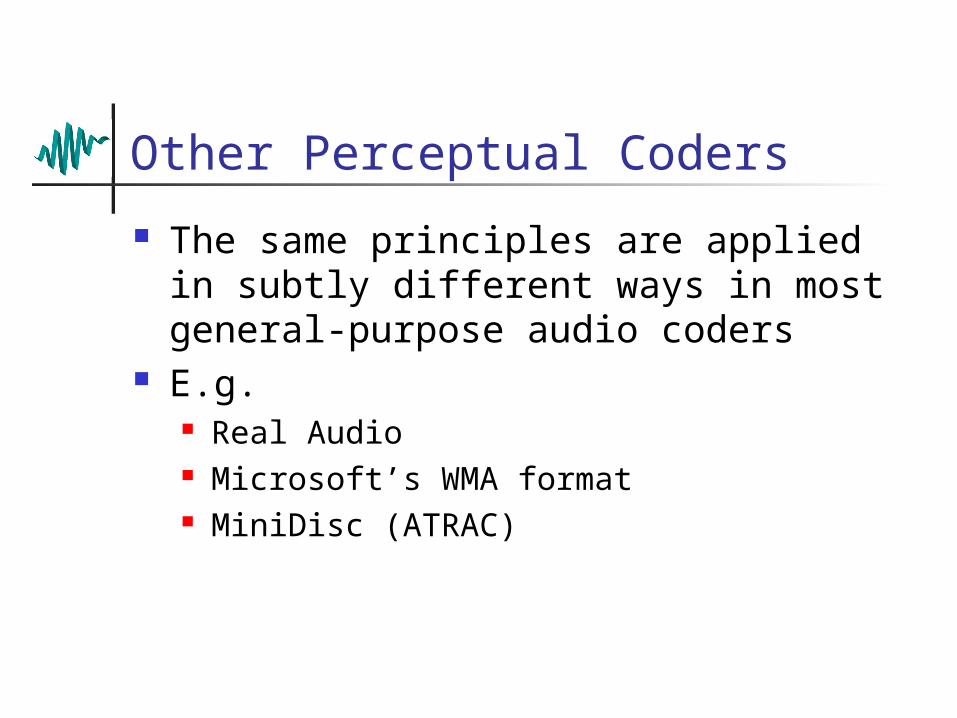
Other Perceptual Coders
The same principles are applied in subtly different ways in most general-purpose audio coders
E.g. Real Audio Microsoft’s WMA format MiniDisc (ATRAC)
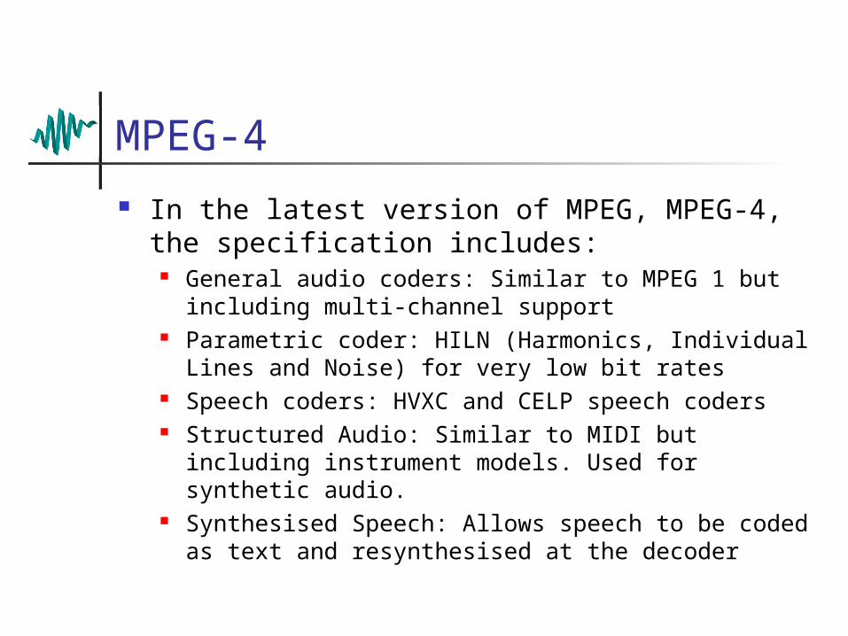
MPEG-4
In the latest version of MPEG, MPEG-4, the specification includes:
General audio coders: Similar to MPEG 1 but including multi-channel support
Parametric coder: HILN (Harmonics, Individual Lines and Noise) for very low bit rates
Speech coders: HVXC and CELP speech coders Structured Audio: Similar to MIDI but including
instrument models. Used for synthetic audio. Synthesised Speech: Allows speech to be coded as
text and resynthesised at the decoder
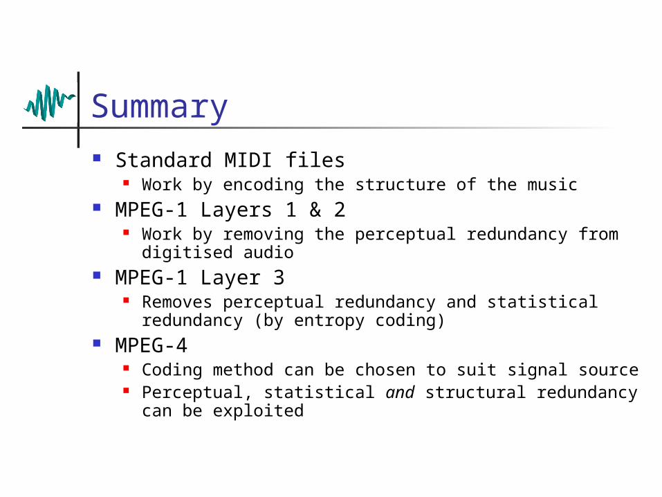
Summary Standard MIDI files
Work by encoding the structure of the music MPEG-1 Layers 1 & 2
Work by removing the perceptual redundancy from digitised audio
MPEG-1 Layer 3 Removes perceptual redundancy and statistical
redundancy (by entropy coding) MPEG-4
Coding method can be chosen to suit signal source Perceptual, statistical and structural redundancy can
be exploited
Related Documents
![EfficientBit AllocationAlgorithmFor MPEG-4 Audio · as MPEG-1/2/4 audio coding standards and Dolby AC-3 [1]. The MPEG-4 Advanced Audio Coding (AAC) is one ofthe mostrecent-generation](https://static.cupdf.com/doc/110x72/5b3b16727f8b9a26728c2604/efficientbit-allocationalgorithmfor-mpeg-4-audio-as-mpeg-124-audio-coding.jpg)