DESIGN AND ANALYSIS OF MEDIUM ACCESS CONTROL PROTOCOLS FOR AD HOC AND COOPERATIVE WIRELESS NETWORKS Ph. D. Dissertation by Jesús Alonso-Zárate Ph. D. Thesis Advisors: Christos Verikoukis, Ph. D. Senior Research Associate Centre Tecnològic de Telecomunicacions de Catalunya (CTTC) Luis Alonso, Ph. D. Associate Professor Department of Signal Theory and Communications (TSC) Escola Politècnica Superior de Castelldefels (EPSC) Universitat Politècnica de Catalunya (UPC) Barcelona, January 2009

Welcome message from author
This document is posted to help you gain knowledge. Please leave a comment to let me know what you think about it! Share it to your friends and learn new things together.
Transcript
DESIGN AND ANALYSIS OF MEDIUM ACCESS CONTROL
PROTOCOLS FOR AD HOC AND COOPERATIVE
WIRELESS NETWORKS
Ph. D. Dissertation by
Jesús Alonso-Zárate
Ph. D. Thesis Advisors:
Christos Verikoukis, Ph. D. Senior Research Associate
Centre Tecnològic de Telecomunicacions de Catalunya (CTTC)
Luis Alonso, Ph. D. Associate Professor
Department of Signal Theory and Communications (TSC) Escola Politècnica Superior de Castelldefels (EPSC)
Universitat Politècnica de Catalunya (UPC)
Barcelona, January 2009


A mi familia.
Para Cris.

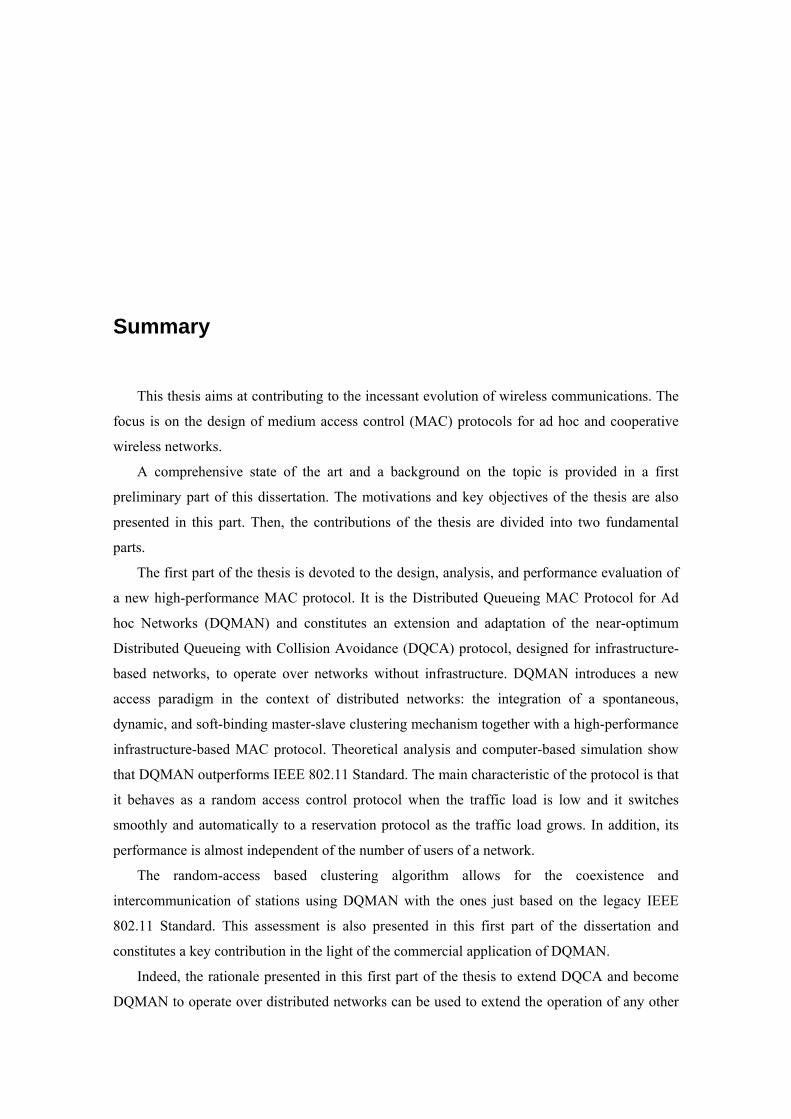
Summary
This thesis aims at contributing to the incessant evolution of wireless communications. The
focus is on the design of medium access control (MAC) protocols for ad hoc and cooperative
wireless networks.
A comprehensive state of the art and a background on the topic is provided in a first
preliminary part of this dissertation. The motivations and key objectives of the thesis are also
presented in this part. Then, the contributions of the thesis are divided into two fundamental
parts.
The first part of the thesis is devoted to the design, analysis, and performance evaluation of
a new high-performance MAC protocol. It is the Distributed Queueing MAC Protocol for Ad
hoc Networks (DQMAN) and constitutes an extension and adaptation of the near-optimum
Distributed Queueing with Collision Avoidance (DQCA) protocol, designed for infrastructure-
based networks, to operate over networks without infrastructure. DQMAN introduces a new
access paradigm in the context of distributed networks: the integration of a spontaneous,
dynamic, and soft-binding master-slave clustering mechanism together with a high-performance
infrastructure-based MAC protocol. Theoretical analysis and computer-based simulation show
that DQMAN outperforms IEEE 802.11 Standard. The main characteristic of the protocol is that
it behaves as a random access control protocol when the traffic load is low and it switches
smoothly and automatically to a reservation protocol as the traffic load grows. In addition, its
performance is almost independent of the number of users of a network.
The random-access based clustering algorithm allows for the coexistence and
intercommunication of stations using DQMAN with the ones just based on the legacy IEEE
802.11 Standard. This assessment is also presented in this first part of the dissertation and
constitutes a key contribution in the light of the commercial application of DQMAN.
Indeed, the rationale presented in this first part of the thesis to extend DQCA and become
DQMAN to operate over distributed networks can be used to extend the operation of any other
infrastructure-based MAC protocol to ad hoc networks. In order to exemplify this, a case study
is presented to conclude the first part of the thesis. The Distributed Point Coordination Function
(DPCF) MAC protocol is presented as the extension of the PCF of the IEEE 802.11 Standard to
be used in ad hoc networks.
The second part of the thesis turns the focus to a specific kind of cooperative
communications: Cooperative Automatic Retransmission Request (C-ARQ) schemes. The main
idea behind C-ARQ is that when a packet is received with errors at a receiver, a retransmission
can be requested not only from the source but also to any of the users which overheard the
original transmission. These users can become spontaneous helpers to assist in the failed
transmission by forming a temporary ad hoc network. Although such a scheme may provide
cooperative diversity gain, involving a number of users in the communication between two
users entails a complicated coordination task that has a certain cost. This cost has been typically
neglected in the literature, assuming that the relays can attain a perfect scheduling and transmit
one after another. In this second part of the thesis, the cost of the MAC layer in C-ARQ
schemes is analyzed and two novel MAC protocols for C-ARQ are designed, analyzed, and
comprehensively evaluated. They are the DQCOOP and the Persistent Relay Carrier Sensing
Multiple Access (PRCSMA) protocols. The former is based on DQMAN and the latter is based
on the IEEE 802.11 Standard. A comparison with non-cooperative ARQ schemes
(retransmissions performed only from the source) and with ideal C-ARQ (with perfect
scheduling among the relays) is included to have actual reference benchmarks of the novel
proposals. The main results show that an efficient design of the MAC protocol is crucial in
order to actually obtain the benefits associated to the C-ARQ schemes.
Resumen
La presente tesis doctoral contribuye a la incesante evolución de las comunicaciones
inalámbricas. Se centra en el diseño de protocolos de acceso al medio (MAC) para redes ad hoc
y redes inalámbricas cooperativas.
En una primera parte introductoria se presenta un minucioso estado del arte y se establecen
las bases teóricas de las contribuciones presentadas en la tesis. En esta primera parte
introductoria se definen las principales motivaciones de la tesis y se plantean los objetivos.
Después, las contribuciones de la tesis se organizan en dos grandes bloques, o partes.
En la primera parte de esta tesis se diseña, analiza y evalúa el rendimiento de un novedoso
protocolo MAC de alta eficiencia llamado DQMAN (Protocolo MAC basado en colas
distribuidas para redes ad hoc). Este protocolo constituye la extensión y adaptación del
protocolo DQCA, diseñado para redes centralizadas, para operar en redes sin infraestructura. En
DQMAN se introduce un nuevo paradigma en el campo del acceso al medio para redes
distribuidas: la integración de un algoritmo de clusterización espontáneo y dinámico basado en
una estructura de master y esclavo junto con un protocolo MAC de alta eficiencia diseñado para
redes centralizadas. Tanto el análisis teórico como las simulaciones por ordenador presentadas
en esta tesis muestran que DQMAN mejora el rendimiento del actual estándar IEEE 802.11. La
principal característica de DQMAN es que se comporta como un protocolo de acceso aleatorio
cuando la carga de tráfico es baja y cambia automática y transparentemente a un protocolo de
reserva a medida que el tráfico de la red aumenta. Además, su rendimiento es prácticamente
independiente del número de usuarios simultáneos de la red, lo cual es algo deseable en redes
que nacen para cubrir una necesidad espontánea y no pueden ser planificadas.
El hecho de que algoritmo de clusterización se base en un acceso aleatorio permite la
coexistencia e intercomunicación de usuarios DQMAN con usuarios basados en el estándar
IEEE 802.11. Este estudio se presenta en esta primera parte de la tesis y es fundamental de cara
a una posible explotación comercial de DQMAN.
La metodología presentada en esta tesis mediante el cual se logra extender la operación de
DQCA a entornos ad hoc sin infraestructura puede ser utilizada para adaptar cualquier otro
protocolo centralizado. Con el objetivo de poner de manifiesto esta realidad, la primera parte de
la tesis concluye con el diseño y evaluación de DPCF como una extensión distribuida del modo
de coordinación centralizado (PCF) del estándar IEEE 802.11 para operar en redes distribuidas.
La segunda parte de la tesis se centra en el estudio de un tipo específico de técnicas
cooperativas: técnicas cooperativas de retransmisión automática (C-ARQ). La idea principal de
las técnicas C-ARQ es que cuando un paquete de datos se recibe con bits erróneos, se solicita
retransmisión, no a la fuente de datos, si no a cualquiera de los usuarios que escuchó la
transmisión original. Estos usuarios se convierten en espontáneos retransmisores que permiten
mejorar la eficiencia de la comunicación. A pesar de que este tipo de esquema puede obtener
diversidad de cooperación, el hecho de implicar a más de un usuario en una comunicación punto
a punto requiere una coordinación que hasta ahora ha sido obviada en la literatura, asumiendo
que los retransmisores pueden coordinarse perfectamente para retransmitir uno detrás de otro.
En esta tesis se analiza y evalúa el coste de coordinación impuesto por la capa MAC y se
identifican los principales retos de diseño que las técnicas C-ARQ imponen al diseño de la capa
MAC. Además, se presenta el diseño y análisis de dos novedosos protocolos MAC para C-
ARQ: DQCOOP y PRCSMA. El primero se basa en DQMAN y constituye una extensión de
este para operar en esquemas C-ARQ, mientras que el segundo constituye la adaptación del
estándar IEEE 802.11 para poder ejecutarse en un esquema C-ARQ. El rendimiento de estos
esquemas se compara en esta tesis tanto con esquemas no cooperativos como con esquemas
ideales cooperativos donde se asume que el MAC es ideal. Los resultados principales muestran
que el diseño eficiente de la capa MAC es esencial para obtener todos los beneficios potenciales
de los esquemas cooperativos.
Acknowledgments
Esta tesis nunca habría podido llegar a ser una realidad sin el soporte del Centre Tecnològic
de Telecomunicacions de Catalunya (CTTC). Quiero agradecer a todo su equipo directivo por
creer en un programa de becas que me ha permitido obtener hoy el grado de doctor.
Quiero agradecer especialmente a mis directores de tesis, Christos Verikoukis y Luis
Alonso, por todo el tiempo que han dedicado durante estos cuatro últimos años para ayudarme a
conseguir acabar una tesis que en algunos momentos daba por perdida. Visto con perspectiva,
cada vez veo más claro que esto es una dura carrera de fondo y es necesario tener a alguien que
te aliente y te guíe para llegar hasta el final.
Por otro lado quiero agradecer a Elli Kartsakli y Alex Cateura por sus valiosas aportaciones
a la tesis. Con el DQ, ¡hasta el infinito y más allá! Del mismo modo, agradecer a Daniel Royo y
a Cristian Crespo por dejarse convencer para acabar sus respectivas carreras echándome una
mano con partes importantes de esta tesis.
Lo que he aprendido durante estos años ha sido una realidad, y lo digo en mayúsculas, en
parte gracias a la inspiración de Jesús Gómez y a la interminable paciencia de David Gregoratti
y al Dr. Nizar Zorba. Gracias por estar siempre con una sonrisa cuando venía a molestaros.
También quiero agradecer a todo el equipo humano del CTTC que ha hecho posible que el
desarrollo de esta tesis sea una agradable experiencia. Y en esto incluyo al CTTC Sports Team
con el que hemos vivido momentos de gloria…pocos, pero muy intensos.
Quiero agradecer a mi familia: mis padres, mis hermanos y mi abuela Tere por estar a mi
lado y permitirme seguir formándome a lo largo de los años. Sin sus esfuerzos y apoyo hoy no
estaría donde estoy.

También quiero agradecer a todos mis amigos más cercanos que han soportado mis quejas y
llantos durante todos estos años sobre lo duro que es ser becario. Sinceramente, espero que las
cosas cambien en el futuro y la elección de dedicarse a la investigación tenga un mejor
reconocimiento social y laboral. A todos los que estáis en esto, ánimo!
Y finalmente, quiero agradecer a Cris por estar siempre ahí y ayudarme en todos los
sentidos a acabar este proyecto. Espero que sigas a mi lado para ayudarme a seguir
conquistando mis metas en el futuro.
Por si me dejo a alguien, quiero agradecer a todo aquél que directa o indirectamente,
consciente o inconscientemente, ha contribuido para que esta tesis sea hoy en día lo que es.
I would like to finish these acknowledgments by expressing my gratitude to Jorge García-
Vidal, Ferran Adelantado, Stavros Toumpis, Marcos Katz, and Periklis Chatzimisios for taking
part of my Ph. D. Defence Committee.
Table of Contents
CHAPTER I..............................................................................................................................................21
1 INTRODUCTION ...........................................................................................................................21
1.1 MOTIVATION .............................................................................................................................21 1.2 BACKGROUND ...........................................................................................................................27
1.2.1 MAC Protocols for Wireless Ad Hoc Networks....................................................................27 1.2.1.1 Evolution of the 802.11 MAC Protocol.................................................................................. 28 1.2.1.2 Hybrid CSMA-TDMA Protocols ............................................................................................. 30 1.2.1.3 MAC Protocols with Busy Tones ........................................................................................... 31 1.2.1.4 Cluster-based MAC Protocols ............................................................................................... 32
1.2.2 Analytical Models for MAC Protocols in Ad hoc Networks .................................................36 1.2.3 Cooperative Communications ..............................................................................................37
1.3 MAIN CONTRIBUTIONS AND STRUCTURE OF THE THESIS ...........................................................39 1.4 DISSEMINATION.........................................................................................................................40 1.5 OTHER RESEARCH CONTRIBUTIONS ..........................................................................................42 1.6 REFERENCES..............................................................................................................................43
CHAPTER II ............................................................................................................................................51
2 FRAMEWORK ...............................................................................................................................51
2.1 INTRODUCTION ..........................................................................................................................51 2.2 MARKOV CHAIN THEORY ..........................................................................................................52
2.2.1 Markov Processes and Markov Chains ................................................................................52 2.2.2 Semi-Markov Processes: Embedded Markov Chains ...........................................................53
2.3 QUEUEING THEORY ...................................................................................................................53 2.3.1 Introduction ..........................................................................................................................53 2.3.2 Kendall’s Notation................................................................................................................54 2.3.3 Stability Condition................................................................................................................54 2.3.4 The M/M/1 Queue.................................................................................................................55 2.3.5 Open Networks of Queues ....................................................................................................56
2.4 COMPUTER SIMULATION ...........................................................................................................57 2.4.1 Motivation.............................................................................................................................57 2.4.2 MACSWIN ............................................................................................................................60
2.4.2.1 Overview ................................................................................................................................... 60 2.4.2.2 The Graphic User Interface (GUI) ......................................................................................... 61 2.4.2.3 The Simulation Engine............................................................................................................ 64
2.5 REFERENCES..............................................................................................................................73
CHAPTER III...........................................................................................................................................75
3 A NOVEL MAC PROTOCOL: DQMAN .....................................................................................75
3.1 INTRODUCTION ..........................................................................................................................75 3.2 CHAPTER STRUCTURE................................................................................................................77 3.3 PREVIOUS CONSIDERATIONS .....................................................................................................77 3.4 CLUSTERING AT THE MAC LAYER ............................................................................................79
3.4.1 Motivation and Overview .....................................................................................................79 3.4.2 Fundamentals and Definitions..............................................................................................79 3.4.3 Cluster Formation and Maintenance....................................................................................80 3.4.4 Setting Up the Value of the MSSI .........................................................................................82 3.4.5 Master Collision Resolution .................................................................................................83 3.4.6 Dynamic Reclustering...........................................................................................................83
3.5 THE MAC PROTOCOL................................................................................................................84 3.5.1 Description ...........................................................................................................................84 3.5.2 The MAC Protocol Rules......................................................................................................86
3.5.2.1 Preliminaries............................................................................................................................. 86 3.5.2.2 QDR (Queueing Discipline Rules)......................................................................................... 89 3.5.2.3 DTR (Data Transmission Rules)............................................................................................ 89 3.5.2.4 RTR (Request Transmission Rules) ..................................................................................... 90
3.6 EXAMPLE OF OPERATION...........................................................................................................90 3.7 GENERAL DISCUSSION...............................................................................................................92
3.7.1 Special Rule: Initialization of a Cluster ...............................................................................92 3.7.2 Avoiding Empty Data Frames ..............................................................................................92 3.7.3 Providing Incentive to Operate in Master Mode ..................................................................94 3.7.4 Implicit Cooperative Operation............................................................................................95 3.7.5 Dual-Distributed ACK Algorithm.........................................................................................95
3.8 PERFORMANCE ANALYSIS IN SINGLE-HOP NETWORKS .............................................................97 3.8.1 Introduction ..........................................................................................................................97 3.8.2 Preliminary Considerations and Definitions ........................................................................97
3.8.2.1 Transmission Rates and Channel Error Model ................................................................... 97 3.8.2.2 Slot and Superslot Time Reference ...................................................................................... 98 3.8.2.3 Throughput Definition.............................................................................................................. 99 3.8.2.4 Average Message Transmission Delay .............................................................................. 100
3.8.3 Analysis in Saturation Conditions ......................................................................................100 3.8.3.1 Overview ................................................................................................................................. 100 3.8.3.2 Clustering Model .................................................................................................................... 101 3.8.3.3 MSSI Counter with Offset: Master Sharing ........................................................................ 103 3.8.3.4 Saturation Throughput Analysis .......................................................................................... 104 3.8.3.5 Model Validation and Performance Evaluation ................................................................. 106 3.8.3.6 Comparison with the IEEE 802.11 MAC Protocol............................................................. 110 3.8.3.7 Conclusions ............................................................................................................................ 112
3.8.4 Analysis in Non-Saturation Conditions ..............................................................................113 3.8.4.1 Overview ................................................................................................................................. 113 3.8.4.2 Clustering Model .................................................................................................................... 114 3.8.4.3 The DQMAN Busy Period .................................................................................................... 117 3.8.4.4 Throughput Analysis ............................................................................................................. 124 3.8.4.5 Clustering Analysis ................................................................................................................ 126 3.8.4.6 Average Message Transmission Delay Analysis .............................................................. 127 3.8.4.7 Model Validation and Performance Evaluation ................................................................. 129 3.8.4.8 Comparison with the IEEE 802.11 MAC Protocol............................................................. 133 3.8.4.9 Conclusions ............................................................................................................................ 135
3.9 PERFORMANCE ENHANCEMENTS .............................................................................................136 3.9.1 Introduction ........................................................................................................................136 3.9.2 Master Cooperation Request (MCR) ..................................................................................136
3.9.2.1 Problem Statement................................................................................................................ 136 3.9.2.2 Proposed Mechanism ........................................................................................................... 137
3.9.3 Advanced MTO Mechanism................................................................................................138 3.9.3.1 Problem Statement................................................................................................................ 138 3.9.3.2 Proposed Mechanism ........................................................................................................... 138
3.9.4 Performance Evaluation.....................................................................................................138 3.9.4.1 Scenario .................................................................................................................................. 139 3.9.4.2 Results .................................................................................................................................... 139
3.9.5 Conclusions ........................................................................................................................142 3.10 PERFORMANCE IN MULTI-HOP NETWORKS .............................................................................143
3.10.1 Introduction....................................................................................................................143 3.10.2 Channel Model ...............................................................................................................144 3.10.3 Performance Discussion ................................................................................................145
3.10.3.1 Blocked Stations ............................................................................................................... 145 3.10.3.2 Exposed Stations .............................................................................................................. 146 3.10.3.3 Hidden and Unreachable Stations.................................................................................. 146
3.10.4 Modifications for Multi-hop Networks ...........................................................................148 3.10.4.1 Tackling with Blocked Stations: Busy Tones and MTO............................................... 148 3.10.4.2 Tackling with Exposed Stations: Active Listening ........................................................ 149 3.10.4.3 Tackling with Hidden and Unreachable Stations: Receiver Initiated Clustering ...... 151
3.10.5 Performance Evaluation ................................................................................................152 3.10.5.1 Network Layout and Scenario Configuration ................................................................ 152
3.10.5.2 Results ............................................................................................................................... 154 3.10.6 Conclusions ....................................................................................................................157
3.11 COEXISTENCE WITH LEGACY IEEE 802.11 NETWORKS...........................................................157 3.11.1 Introduction....................................................................................................................157 3.11.2 Overview ........................................................................................................................158 3.11.3 Scenario .........................................................................................................................158 3.11.4 Coexistence Methodology ..............................................................................................159 3.11.5 Performance Evaluation ................................................................................................162
3.11.5.1 Scenario ............................................................................................................................. 162 3.11.5.2 Results ............................................................................................................................... 163
3.11.6 Conclusions ....................................................................................................................166 3.12 CHAPTER CONCLUSIONS..........................................................................................................166 3.13 REFERENCES............................................................................................................................168
CHAPTER IV.........................................................................................................................................173
4 A NOVEL MAC PROTOCOL: DPCF........................................................................................173
4.1 INTRODUCTION ........................................................................................................................173 4.2 CHAPTER STRUCTURE..............................................................................................................174 4.3 IEEE 802.11 MAC PROTOCOL OVERVIEW..............................................................................174
4.3.1 DCF Overview....................................................................................................................174 4.3.2 PCF Overview ....................................................................................................................176
4.4 A NEW MAC PROTOCOL: DPCF .............................................................................................177 4.4.1 Protocol Description ..........................................................................................................178 4.4.2 Performance Evaluation in Single-Hop Networks..............................................................182
4.4.2.1 Scenario .................................................................................................................................. 182 4.4.2.2 Results .................................................................................................................................... 183
4.4.3 Performance Evaluation in Multi-hop Networks................................................................188 4.4.3.1 Scenario .................................................................................................................................. 188 4.4.3.2 Results .................................................................................................................................... 189
4.5 COEXISTENCE WITH LEGACY IEEE 802.11 NETWORKS...........................................................191 4.5.1.1 Introduction ............................................................................................................................. 191 4.5.1.2 Coexistence Methodology .................................................................................................... 191 4.5.1.3 Performance Evaluation ....................................................................................................... 193
4.6 PERFORMANCE COMPARISON WITH DQMAN .........................................................................196 4.6.1 Scenario..............................................................................................................................196 4.6.2 Results ................................................................................................................................197
4.7 CHAPTER CONCLUSIONS..........................................................................................................199 4.8 REFERENCES............................................................................................................................200
CHAPTER V ..........................................................................................................................................201
5 COOPERATIVE ARQ: DQCOOP AND PRCSMA ..................................................................201
5.1 INTRODUCTION ........................................................................................................................201 5.1.1 Cooperative ARQ (C-ARQ) ................................................................................................203
5.1.1.1 Background and Motivation.................................................................................................. 203 5.1.1.2 Description.............................................................................................................................. 204 5.1.1.3 Discussion .............................................................................................................................. 206
5.1.2 Motivation and Contributions of the Chapter.....................................................................209 5.1.3 Related work: Cooperative MAC Protocols .......................................................................211
5.2 DQMAN FOR C-ARQ: DQCOOP...........................................................................................213 5.2.1 Introduction and Problem Statement..................................................................................213 5.2.2 Protocol Description ..........................................................................................................216
5.2.2.1 Clustering Algorithm .............................................................................................................. 217 5.2.2.2 The MAC Protocol: Frame Structure and Protocol Rules ................................................ 218
5.2.3 Operational Example..........................................................................................................219 5.2.4 Cooperation Delay Analysis ...............................................................................................221 5.2.5 Model Validation and Performance Evaluation .................................................................224
5.2.5.1 Model Validation .................................................................................................................... 225 5.2.5.2 Number of Minislots within the Cooperation Phase (m) ................................................... 226 5.2.5.3 Number of Minislots of the Start-up Phase (m0)................................................................ 228
5.2.6 Conclusions ........................................................................................................................230 5.3 PRCSMA: PERSISTENT RELAY CSMA PROTOCOL .................................................................231
5.3.1 Introduction and Problem Statement..................................................................................231 5.3.2 Protocol Description ..........................................................................................................232 5.3.3 Operational Example..........................................................................................................233 5.3.4 Cooperation Delay Analysis ...............................................................................................234
5.3.4.1 Introduction ............................................................................................................................. 234 5.3.4.2 PRCSMA Model..................................................................................................................... 235 5.3.4.3 Contention Delay Analysis ................................................................................................... 239
5.3.5 Model Validation and Performance Evaluation .................................................................241 5.3.5.1 Scenario .................................................................................................................................. 241 5.3.5.2 Results .................................................................................................................................... 242
5.3.6 Conclusions ........................................................................................................................246 5.4 C-ARQ VS. NON-COOP. ARQ: PERFORMANCE COMPARISON .................................................247
5.4.1 Introduction ........................................................................................................................247 5.4.2 Performance Evaluation.....................................................................................................248 5.4.3 Conclusions ........................................................................................................................250
5.5 CASE STUDY: ROOFTOP AP NETWORK WITH C-ARQ..............................................................251 5.5.1 Introduction ........................................................................................................................251 5.5.2 System Model......................................................................................................................252 5.5.3 Throughput Analysis...........................................................................................................256
5.5.3.1 Throughput with Traditional Non-Cooperative ARQ ......................................................... 256 5.5.3.2 Throughput with C-ARQ ....................................................................................................... 257
5.5.4 Performance Evaluation.....................................................................................................258 5.5.4.1 Introduction ............................................................................................................................. 258 5.5.4.2 Model Validation .................................................................................................................... 259 5.5.4.3 Packet Error Probability in the Channel from Source to Destination.............................. 260 5.5.4.4 Packet Error Probability in the Channel from Relays to Destination .............................. 263 5.5.4.5 The Number of Active Relays .............................................................................................. 266 5.5.4.6 Data Transmission Rates ..................................................................................................... 267
5.5.5 Conclusions ........................................................................................................................269 5.6 CHAPTER CONCLUSIONS..........................................................................................................270 5.7 REFERENCES............................................................................................................................272
CHAPTER VI.........................................................................................................................................277
6 CONCLUSIONS AND FUTURE WORK...................................................................................277
6.1 SUMMARY AND CONCLUSIONS ................................................................................................277 6.2 FUTURE WORK ........................................................................................................................281
List of Figures
Figure 1.1 Example of Ad Hoc Network .................................................................................... 22 Figure 1.2 Example: Cooperative Scenario................................................................................. 25 Figure 1.3 Cooperative Transmissions in Two Time Slots ......................................................... 26 Figure 1.4 Clustering in Ad Hoc Networks................................................................................. 32 Figure 1.5 Cooperative Relay Network....................................................................................... 38 Figure 2.1 Queueing System with One Server ............................................................................ 54 Figure 2.2 M/M/1 Markov Chain................................................................................................ 55 Figure 2.3 Examples of Open and Closed Network of Queues................................................... 56 Figure 2.4 MACSWIN and the OSI Layer Model ...................................................................... 60 Figure 2.5 Configuration of a Simulation in MACSWIN ........................................................... 62 Figure 2.6 Configuration of a Nested Battery of Sequential Simulations in MACSWIN........... 62 Figure 2.7 Screenshot of MACSWIN ......................................................................................... 63 Figure 2.8 Main Loop of the Simulation in MACSWIN ............................................................ 64 Figure 2.9 Relationship between Mobile Classes in MACSWIN ............................................... 66 Figure 2.10 Instances of the Classes in a Basic Simulation ........................................................ 66 Figure 2.11 Wireless Channel Modeling in MACSWIN ............................................................ 67 Figure 2.12 Simplified Multiple State-Machine of an 802.11 Station ....................................... 72 Figure 3.1 Concept Design of DQMAN ..................................................................................... 76 Figure 3.2 Fragmentation at the MAC layer ............................................................................... 78 Figure 3.3 DQMAN Clustering Flowchart of a Single Station ................................................... 81 Figure 3.4 Clustering + MAC Structure...................................................................................... 81 Figure 3.5 DQMAN Frame Structure ......................................................................................... 85 Figure 3.6 Distributed Queueing Operation of DQMAN............................................................ 88 Figure 3.7 FBP Payload Format .................................................................................................. 88 Figure 3.8 DQMAN Example of Operation................................................................................ 93 Figure 3.9 Avoiding the Occurrence of Empty Data Frames...................................................... 94 Figure 3.10 Dual-Distributed ACK Mechanism of DQMAN..................................................... 96 Figure 3.11 Slot and Superslot Definition................................................................................... 99 Figure 3.12 States of a Single-hop DQMAN Network ............................................................... 99 Figure 3.13 Markov Chain for the MSSI Counter of a Station in Saturation Conditions ......... 101 Figure 3.14 Probability that a Master does not Become Master in the Next MSS (PN)............ 105 Figure 3.15 Model Validation (DQMAN Saturation Throughput) ........................................... 107 Figure 3.16 Percentage of Time Devoted to Clustering (Contention)....................................... 108 Figure 3.17 Probability of Collision for F=10 and =32........................................................ 109 Figure 3.18 DQMAN Saturation Throughput with Different Values of .............................. 109 Figure 3.19 IEEE 802.11 vs. DQMAN Saturation Throughput ................................................ 112 Figure 3.20 States of a Single-hop DQMAN Network ............................................................. 114 Figure 3.21 Markov Chain Model under Non-Saturation Conditions (DQMAN) .................... 115 Figure 3.22 DQMAN Queueing Model .................................................................................... 118 Figure 3.23 Probability of Finding at Least One Empty Minislot in a Frame........................... 120 Figure 3.24 Simplified DQMAN Queueing Model for Average Busy Period Duration........... 125 Figure 3.25 Reduction of the Average Contention Delay for Masters...................................... 128 Figure 3.26 Non-Saturated Throughput of DQMAN (Model vs. Simulation).......................... 131 Figure 3.27 Percentage of Time in Master Mode (Model vs. Simulation)................................ 132 Figure 3.28 Percentage of Time in Idle or Slave Mode (Model vs. Simulation) ...................... 132
Figure 3.29 Average Message Transmission Delay (Model vs. Simulation)............................ 132 Figure 3.30 Throughput Comparison DQMAN vs. IEEE 802.11............................................. 134 Figure 3.31 Average Message Transmission Delay DQMAN vs. IEEE 802.11....................... 134 Figure 3.32 Master Cooperation Request Flowchart................................................................. 137 Figure 3.33 Average Time Devoted to Clustering .................................................................... 140 Figure 3.34 Aggregate Network Throughput ............................................................................ 140 Figure 3.35 Average Duration of a Master Busy Period........................................................... 141 Figure 3.36 Averages Message Transmission Delay DQMAN vs. DQMAN+ ........................ 142 Figure 3.37 Jain Index of the Average Message Transmission Delay ...................................... 142 Figure 3.38 Transmission and Interference Ranges .................................................................. 145 Figure 3.39 S1 is a Blocked Station between Masters M1 and M2 .......................................... 146 Figure 3.40 S2 is an Exposed Station........................................................................................ 146 Figure 3.41 Hidden stations ...................................................................................................... 147 Figure 3.42 Unreachable stations .............................................................................................. 147 Figure 3.43 3 hops between Adjacent Masters Reduce the Problem of Blocked Stations........ 149 Figure 3.44 DQMAN Frame Structure with ACK_AL............................................................. 150 Figure 3.45 ACK_AL Mechanism Flowchart (data reception)................................................. 150 Figure 3.46 DQMAN-RI Flowchart.......................................................................................... 151 Figure 3.47 Example of DQMAN-RI Operation....................................................................... 152 Figure 3.48 Multi-hop Network Layout .................................................................................... 153 Figure 3.49 Throughput to Destination ..................................................................................... 155 Figure 3.50 Average Packet Transmission Delay ..................................................................... 155 Figure 3.51 Ratio of Traffic Delivered in Active Listening...................................................... 155 Figure 3.52 Throughput to Destination ..................................................................................... 156 Figure 3.53 Ratio of Traffic Delivered in Active Listening...................................................... 156 Figure 3.54 Average Packet Transmission Delay (ms) ............................................................. 157 Figure 3.55 Format of RTS and CTS packets ........................................................................... 159 Figure 3.56 Receiver Initiated DQMAN for Coexistence with the Standard............................ 160 Figure 3.57 Receiver Flowchart in the Coexistence Scenario (DQMAN-DCF)....................... 160 Figure 3.58 Standard Periods Follow DQMAN Periods in a Coexistence Scenario................. 161 Figure 3.59 Throughput in a Mixed Network ........................................................................... 163 Figure 3.60 Throughput Attained by Each Group of Stations .................................................. 164 Figure 3.61 Average Packet Transmission Delay ..................................................................... 165 Figure 3.62 Jain Index of the Average Packet Transmission Delay in Coexistence Scenarios 165 Figure 4.1 IEEE 802.11 DCF Basic Access.............................................................................. 175 Figure 4.2 IEEE 802.11 DCF Collision Avoidance Access (RTS/CTS) .................................. 175 Figure 4.3 PCF is Comprised of Contention Free Periods and Contention Periods.................. 176 Figure 4.4 IEEE 802.11 PCF Example of Operation ................................................................ 177 Figure 4.5 DPCF Inspired by DQMAN .................................................................................... 178 Figure 4.6 DPCF Example of Operation ................................................................................... 179 Figure 4.7 Beacons, Polls, and MTO in DPCF ......................................................................... 180 Figure 4.8 MIFS Definition in DPCF (Maximum Time between Two Consecutive Polls)...... 181 Figure 4.9 A Backoff is executed after a CFP Period to Avoid Collisions ............................... 181 Figure 4.10 DPCF Flowchart .................................................................................................... 182 Figure 4.11 Throughput Comparison DPCF, PCF, and DCF.................................................... 184 Figure 4.12 Probability of Transmitting when Being Polled .................................................... 184 Figure 4.13 Polls Transmitted per Second by the AP and Average Number of Polls per Seconds Received by Regular Stations in the PCF and the DPCF networks .......................................... 185 Figure 4.14 Average Number of Polls per Second Received per Station ................................. 186 Figure 4.15 Probability of Transmitting when Being Polled .................................................... 186 Figure 4.16 Average Packet Transmission Delay ..................................................................... 187 Figure 4.17 Multi-hop Scenario for DPCF................................................................................ 188 Figure 4.18 Throughput to Destination of DPCF in a Multihop Network ................................ 190 Figure 4.19 Average Packet Transmission Delay of DPCF in Multihop Network ................... 190 Figure 4.20 Reception Flowchart in the Coexistence Scenario (DPCF-DCF) .......................... 192

Figure 4.21 DCF Periods Follow CFPs in a Coexistence Scenario .......................................... 192 Figure 4.22 Throughput in Mixed Scenarios DPCF-DCF ........................................................ 195 Figure 4.23 Throughput DCF-only Stations in the Mixed Scenario ......................................... 195 Figure 4.24 Throughput DPCF Stations in the Mixed Scenario ............................................... 195 Figure 4.25 Average Packet Transmission Delay in Mixed Scenarios DPCF-DCF ................. 196 Figure 4.26 Throughput of DQMAN vs. DPCF........................................................................ 198 Figure 4.27 Average Packet Transmission Delay of DQMAN vs. DPCF ................................ 198 Figure 5.1 C-ARQ Flowchart.................................................................................................... 206 Figure 5.2 C-ARQ Scheme with Time-Orthogonal Relays ...................................................... 206 Figure 5.3 Flowchart of the Cooperation Phase Initialization with Relay Selection Criteria ... 207 Figure 5.4 Master-Slave Architecture of DQCOOP (simplified example) ............................... 214 Figure 5.5 Average Number of Empty Frames (DQMAN) ...................................................... 215 Figure 5.6 Clustering Algorithm DQMAN vs. DQCOOP ........................................................ 217 Figure 5.7 DQCOOP MAC Frame Structure ............................................................................ 218 Figure 5.8 DQCOOP Example of Operation............................................................................. 220 Figure 5.9 Probability of having at Least one Success in the First Frame ................................ 223 Figure 5.10 Validation of the Model (DQCOOP)..................................................................... 225 Figure 5.11 Average Packet Transmission Delays for Different Values of m0=m ................... 226 Figure 5.12 Average Packet Transmission Delay for Different Values of m=m0..................... 227 Figure 5.13 Average Packet Transmission Times for Different Values of K ........................... 227 Figure 5.14 Protocol Relative Overhead (DQCOOP) ............................................................... 229 Figure 5.15 Average Packet Transmission Delay as a Function of m0 ..................................... 229 Figure 5.16 PRCSMA Example of Operation........................................................................... 233 Figure 5.17 Markov Chain of a PRCSMA Station.................................................................... 236 Figure 5.18 PRCSMA Model Validation (Basic and COLAV Access).................................... 243 Figure 5.19 Average Packet Transmission Delay (PRCSMA with basic access) ..................... 245 Figure 5.20 Average Packet Transmission Delay (PRCSMA with COLAV access) ............... 245 Figure 5.21 PRCSMA Average Packet Transmission Delay with Different CWs ................... 245 Figure 5.22 Difference in the Calculation of the Model for COLAV Access with BEB.......... 246 Figure 5.23 Comparison C-ARQ: Average Packet Transmission Delay .................................. 249 Figure 5.24 Comparison DQCOOP vs. PRCSMA (K=1)......................................................... 249 Figure 5.25 Comparison DQCOOP vs. PRCSMA (K=2)......................................................... 249 Figure 5.26 Rooftop AP scenario .............................................................................................. 252 Figure 5.27 Cooperative Scenario ............................................................................................. 253 Figure 5.28 Two-State Markov Model for the Rayleigh Channel............................................. 254 Figure 5.29 Throughput Model Validation Network with C-ARQ (Rooftop AP) .................... 260 Figure 5.30 Throughput Comparison for pRD=0.1 (Rooftop AP).............................................. 261 Figure 5.31 Throughput Comparison for pRD=0.7 (Rooftop AP).............................................. 263 Figure 5.32 Throughput Comparison for pSD=0.1 (Rooftop AP).............................................. 264 Figure 5.33 Throughput Comparison for pSD=0.7 (Rooftop AP) .............................................. 265 Figure 5.34 Throughput Comparison for Different Number of Active Relays (Rooftop AP) .. 266 Figure 5.35 Throughput Comparison for Different Number of Active Relays (Rooftop AP) .. 267 Figure 5.36 Throughput Comparison for Different Data Transmission Rates (Rooftop AP) ... 268 Figure 5.37 Throughput Augmentation for Different Data Transmission Rates (Rooftop AP) 268

List of Acronyms
ACK Acknowledgment ACK_AL Acknowledgment in Active Listening AL Active Listening AP Access Point ARQ Automatic Retransmission/Repeat Request ARS Access Request Sequence BEB Binary Exponential Backoff C-ARQ Cooperative ARQ CCA Clear Channel Assessment CDMA Code Division Multiple Access CFC Call for Cooperation CRC Cyclic Redundancy Code CRQ Collision Resolution Queue CSMA Carrier Sensing Multiple Access CSMA/CA Carrier Sensing Multiple Access with Collision Avoidance CTS Clear to Send DBE Detailed Balance Equations DCF Distributed Coordination Function DIFS DCF Inter Frame Space DPCF Distributed Point Coordination Function DQCA Distributed Queueing with Collision Avoidance DQCOOP DQMAN for Cooperative ARQ DQMAN Distributed Queueing MAC protocol for Ad Hoc Networks DSSS Direct Sequence Spread Spectrum DTQ Data Transmission Queue ED Error Detection FBP FeedBack Packet FEC Forward Error Correction GUI Graphic User Interface IMSI Initial Master Sensing Interval IEEE Institute of Electrical and Electronics Engineers ISM Industrial, Scientific, and Medical free-license band ISO International Standards Organization LAN Local Area Network MAC Medium Access Control MACSWIN The MAC Simulator for Wireless Networks MCR Master Cooperation Request MIFS Maximum Inter Frame Space MIMO Multiple Input Multiple Output MRAC Multiple Relay Access Control MSP Master Selection Phase MSS Master Service Set MSSI Master Sensing Selection Interval MTO Master Time-Out NAV Network Allocation Vector
OSI Open System Interconnection PAN Personal Area Network PCF Point Coordination Function PDA Personal Digital Agenda PHY Physical Layer PIFS PCF Inter Frame Space QoS Quality of Service RTS Request to Send SIFS Short Inter Frame Space SNIR Signal to Noise plus Interference Ratio SNR Signal to Noise Ratio STC Space-Time Codes TDMA Time Division Multiple Access WLAN Wireless LAN WWRF Wireless World Research Forum
21
Chapter I
1 Introduction
1.1 Motivation
The world has witnessed an outstanding growth of wireless communications over the last
recent years. According to the Wireless World Research Forum (WWRF), by the year 2017,
there will be seven trillion short-range wireless devices serving seven billion people [1].
Technologies are evolving to an internet-based orientation and to break with the tether of the
wires. Users want to be connected wherever, whenever, and with any of the devices that they
have at hand such as laptops, Personal Digital Agendas (PDA’s), MP3 players, portable gaming
consoles, mobile phones, etc. One of the main interests of these users is focused on
interconnecting all these devices with each other in order to share information among them and
also to be connected with the rest of the world, typically via the Internet. In addition, the
extensive use of multimedia content (for example, the video streaming popularized by youtube)
leads to more demanding requirements in terms of bandwidth and Quality of Service (QoS) that
should be met to satisfy the end user.
Chapter I 22
In order to catch up with the extremely fast evolution of the wireless market, it is necessary
to further develop technology at a wide range of interesting topics. These include the
development of more efficient long-life batteries, the further miniaturization of the devices, and
the redesign of the whole communications protocol stack.
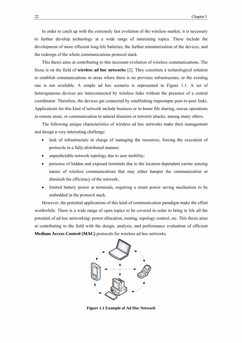
This thesis aims at contributing to this incessant evolution of wireless communications. The
focus is on the field of wireless ad hoc networks [2]. They constitute a technological solution
to establish communications in areas where there is no previous infrastructure, or the existing
one is not available. A simple ad hoc scenario is represented in Figure 1.1. A set of
heterogeneous devices are interconnected by wireless links without the presence of a central
coordinator. Therefore, the devices get connected by establishing impromptu peer-to-peer links.
Applications for this kind of network include business or in-home file sharing, rescue operations
in remote areas, or communication in natural disasters or terrorist attacks, among many others.
The following unique characteristics of wireless ad hoc networks make their management
and design a very interesting challenge:
lack of infrastructure in charge of managing the resources, forcing the execution of
protocols in a fully-distributed manner;
unpredictable network topology due to user mobility;
presence of hidden and exposed terminals due to the location-dependant carrier sensing
nature of wireless communications that may either hamper the communication or
diminish the efficiency of the network;
limited battery power at terminals, requiring a smart power saving mechanism to be
embedded in the protocol stack.
However, the potential applications of this kind of communication paradigm make the effort
worthwhile. There is a wide range of open topics to be covered in order to bring to life all the
potential of ad hoc networking: power allocation, routing, topology control, etc. This thesis aims
at contributing to the field with the design, analysis, and performance evaluation of efficient
Medium Access Control (MAC) protocols for wireless ad hoc networks.
Figure 1.1 Example of Ad Hoc Network
Introduction
23
MAC protocols constitute the set of rules that the users of a network must obey to share a
common communication channel in order to get an efficient use of the available bandwidth,
which is typically scarce [3]. The radio spectrum is not scarce in nature, but the current grid-
lock spectrum assignment allocates different bounded frequency bands for different
applications, limiting the resources available for each one. To make things worse, most of the
wireless communication systems, such as the widely spread IEEE 802.11 Standard for Wireless
Local Area Networks (WLANs), are allocated in the ISM band (Industrial, Scientific, and
Medical), which is shared with many other applications that require or interfere with the use of
the radio spectrum (e.g., microwave ovens operate in this frequency).
Therefore, any MAC protocol should i) avoid or minimize collisions among users, ii)
efficiently handle them in case of occurrence, and iii) avoid a misuse of the resources due to
unnecessary silence periods (deferral periods) in order to obtain the maximum capacity of the
system and to reduce the interference to other systems. In addition, an efficient MAC protocol
should:
1) Ensure a certain degree of fairness among the contending users.
2) Be reliable and stable regardless of the traffic or the number of users of the system.
3) Efficiently manage the power consumption, since typically wireless devices are
equipped with batteries.
4) Be able to provide some degree of QoS to cope with the growing popularity of
multimedia applications, combining video, voice, and data.
The MAC protocol plays a key role in the performance of wireless communications.
Probably for this reason an overwhelming amount of MAC protocols have been proposed in the
literature within the context of wireless ad hoc networks. There are some survey papers which
attempt to summarize the major contributions, such as [4], [5], and [6]. Most of the existing
proposals are based on optimizing a particular set of measures for a particular application, but
none of them have been developed with a general perspective. Therefore, there is still an open
challenge towards the development of totally self-configuring MAC protocols that can meet the
requirements of a wide range of applications. In addition, new technologies and communication
strategies pose new challenges to the design of MAC protocols and thus research at the MAC
layer is one of the most active areas in the communications field.
Having this in mind, this thesis aims at contributing to the field of MAC protocols for
wireless ad hoc networks at two different levels, presented in this thesis as two main connected
parts. The first main part is comprised of Chapters III and IV, and the second main part is
comprised of Chapter V. Chapter II is devoted to providing a background on the topic and the
tools used throughout the development of the thesis.
In Chapter III, the design, analysis, and performance evaluation of a novel MAC protocol
called the Distributed Queueing MAC protocol for Ad hoc Networks (DQMAN) is presented.
Chapter I 24
This protocol constitutes an extension and adaptation of the near-optimum Distributed Queueing
with Collision Avoidance (DQCA) MAC protocol, designed for infrastructure-based WLANs
and presented in [7], for its operation in infrastructureless wireless networks. The key of the
high performance of DQCA is that it behaves as a random access protocol when the traffic load
is low and it switches smoothly and automatically to a reservation protocol as the traffic load
grows. Therefore, it attains the better of the two access methods, i.e., short transmission delays
for low traffic loads, and high throughput under heavy traffic conditions. This hybrid and
dynamic seamless transition turns the protocol into a good candidate for the highly dynamic
environment of ad hoc networks. However, DQCA requires the presence of a central
coordinator. The approach in DQMAN is to integrate DQCA into a passive, spontaneous,
temporary, and soft-binding master-slave clustering algorithm based on Carrier Sensing
Multiple Access (CSMA) [8]. The main idea is that the users of a network get spontaneously
self-organized into impromptu temporary hierarchical clusters only when there is data to
transmit. Within each cluster, one user adopts the role of central indirect coordinator for
bounded periods of time and a modified version of DQCA is executed. Despite the hierarchical
structure, all the communications are performed by establishing peer-to-peer links. A
comprehensive description of DQMAN is presented in this thesis. Two analytical models to
evaluate both the saturation throughput and the performance of DQMAN under arbitrary non-
saturated conditions are also developed. This latter model allows computing the throughput, the
average message transmission delay, and the performance of the clustering mechanism with
different metrics as a function of the offered traffic load. The accuracy of the two models is
assessed by means of comparing the numerical results with the ones obtained from computer
simulations carried out with a custom-made object-oriented C++ software simulator where the
protocol operation is executed (and no formulae are used at the MAC level). The software
simulator is named MACSWIN and its development has been tackled throughout the course of
this thesis. The simulator is described in detail in Chapter II.
Indeed, the rationale behind DQMAN in order to extend and adapt DQCA to
infrastructureless networks can be also applied to any other infrastructure-based MAC protocol.
In order to exemplify this, the first main part of the thesis is completed in Chapter IV with the
design and performance evaluation of the Distributed Point Coordination Function (DPCF)
protocol. DPCF is presented as an extension and adaptation of the Point Coordination Function
(PCF) of the IEEE 802.11 Standard [9] to operate in distributed networks without infrastructure
following the same ideas used to extend DQCA to become DQMAN. In other words, DPCF is
to the PCF of the standard what DQMAN is to DQCA. The performance of DPCF is also
evaluated using MACSWIN.
The second main part of the thesis turns the focus to a specific MAC problem that comes up
within the context of cooperative communications [10]. These techniques are deemed to create
Introduction
25
a revolution in wireless communication networks by exploiting the broadcast nature of the
wireless channel. Since the air interface is a common communication channel that is shared
among all the users in a wireless network, all the transmissions can be potentially overheard by
any user in the system. As a consequence, users can cooperate with each other to provide
independent transmission paths and thus to attain cooperative diversity. A generalized point of
view is that cooperative communications constitute a feasible solution to overcome the practical
implementation problems found when attempting to implement MIMO (Multiple Input Multiple
Output) techniques with relatively small devices, where the maximum distance between
antennas is constrained by the size of the devices.
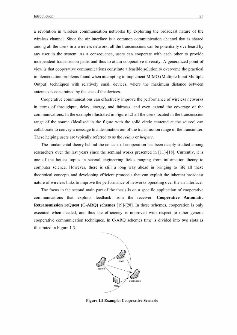
Cooperative communications can effectively improve the performance of wireless networks
in terms of throughput, delay, energy, and fairness, and even extend the coverage of the
communications. In the example illustrated in Figure 1.2 all the users located in the transmission
range of the source (idealized in the figure with the solid circle centered at the source) can
collaborate to convey a message to a destination out of the transmission range of the transmitter.
These helping users are typically referred to as the relays or helpers.
The fundamental theory behind the concept of cooperation has been deeply studied among
researchers over the last years since the seminal works presented in [11]-[18]. Currently, it is
one of the hottest topics in several engineering fields ranging from information theory to
computer science. However, there is still a long way ahead in bringing to life all these
theoretical concepts and developing efficient protocols that can exploit the inherent broadcast
nature of wireless links to improve the performance of networks operating over the air interface.
The focus in the second main part of the thesis is on a specific application of cooperative
communications that exploits feedback from the receiver: Cooperative Automatic
Retransmission reQuest (C-ARQ) schemes [19]-[28]. In these schemes, cooperation is only
executed when needed, and thus the efficiency is improved with respect to other generic
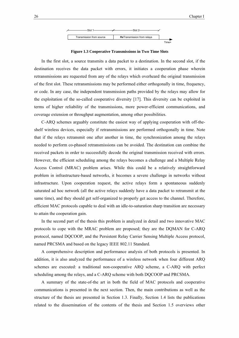
cooperative communication techniques. In C-ARQ schemes time is divided into two slots as
illustrated in Figure 1.3.
relay
destination
relay
source
Figure 1.2 Example: Cooperative Scenario
Chapter I 26
Transmission from source
Time+
ReTransmission from relays
Slot 1 Slot 2
Figure 1.3 Cooperative Transmissions in Two Time Slots
In the first slot, a source transmits a data packet to a destination. In the second slot, if the
destination receives the data packet with errors, it initiates a cooperation phase wherein
retransmissions are requested from any of the relays which overheard the original transmission
of the first slot. These retransmissions may be performed either orthogonally in time, frequency,
or code. In any case, the independent transmission paths provided by the relays may allow for
the exploitation of the so-called cooperative diversity [17]. This diversity can be exploited in
terms of higher reliability of the transmissions, more power-efficient communications, and
coverage extension or throughput augmentation, among other possibilities.
C-ARQ schemes arguably constitute the easiest way of applying cooperation with off-the-
shelf wireless devices, especially if retransmissions are performed orthogonally in time. Note
that if the relays retransmit one after another in time, the synchronization among the relays
needed to perform co-phased retransmissions can be avoided. The destination can combine the
received packets in order to successfully decode the original transmission received with errors.
However, the efficient scheduling among the relays becomes a challenge and a Multiple Relay
Access Control (MRAC) problem arises. While this could be a relatively straightforward
problem in infrastructure-based networks, it becomes a severe challenge in networks without
infrastructure. Upon cooperation request, the active relays form a spontaneous suddenly
saturated ad hoc network (all the active relays suddenly have a data packet to retransmit at the
same time), and they should get self-organized to properly get access to the channel. Therefore,
efficient MAC protocols capable to deal with an idle-to-saturation sharp transition are necessary
to attain the cooperation gain.
In the second part of the thesis this problem is analyzed in detail and two innovative MAC
protocols to cope with the MRAC problem are proposed; they are the DQMAN for C-ARQ
protocol, named DQCOOP, and the Persistent Relay Carrier Sensing Multiple Access protocol,
named PRCSMA and based on the legacy IEEE 802.11 Standard.
A comprehensive description and performance analysis of both protocols is presented. In
addition, it is also analyzed the performance of a wireless network when four different ARQ
schemes are executed: a traditional non-cooperative ARQ scheme, a C-ARQ with perfect
scheduling among the relays, and a C-ARQ scheme with both DQCOOP and PRCSMA.
A summary of the state-of-the art in both the field of MAC protocols and cooperative
communications is presented in the next section. Then, the main contributions as well as the
structure of the thesis are presented in Section 1.3. Finally, Section 1.4 lists the publications
related to the dissemination of the contents of the thesis and Section 1.5 overviews other
Introduction
27
research contributions made along the development of the thesis but which have not been
included in this dissertation.
1.2 Background
This thesis is mainly focused on the design and analysis of novel MAC protocols for
wireless ad hoc networks. Therefore, Section 1.2.1 attempts to summarize the main
contributions in the field of MAC protocols for wireless ad hoc networks, while Section 1.2.2
overviews the existing analytical models for these protocols. As aforementioned, there are a vast
number of MAC protocols available in the literature. Therefore, it is not the aim of this section
to provide an exhaustive state-of-the-art of MAC protocols for wireless ad hoc networks, which
can be found in many books and survey papers, such as in [29]. Instead, the aim of this section
is to overview the most representative works related to the topic of this thesis so that the
contribution herein presented can be properly stated and identified.
On the other hand, since the second part of the thesis is focused on cooperative
communications, the fundamental research in this area is reviewed in Section 1.2.3.
Henceforth, and as reported in the literature, the terms user, station, or node of the network
will be interchangeably used to refer to the same concept of a wireless communication device
forming part of a communications network.
1.2.1 MAC Protocols for Wireless Ad Hoc Networks
In totally distributed networks with a common transmitting medium (the radio channel),
stations must decide by themselves when they are able to transmit. While collisions should be
avoided, the spectral efficiency must be maximized, leading to two conflicting targets. The role
of MAC protocols is to establish the set of rules that stations follow in order to decide when
they can get access to the shared medium and to balance the aforementioned tradeoff.
An overwhelming amount of MAC protocols have been designed within the context of
wireless ad hoc networks. The most representative protocols related to the work presented in
this thesis can be classified into four groups:
1) Protocols that evolve from the Distributed Coordination Function (DCF) defined in the
IEEE 802.11 Standard for WLANs. These protocols use dynamic power control,
dynamic carrier sensing, and modified backoff algorithms to improve the performance
of the legacy standard.
2) Hybrid CSMA-Time Division Multiple Access (TDMA) protocols.
3) MAC protocols based on busy tones.
4) Cluster-based MAC protocols, including multi-channel protocols.
Chapter I 28
MAC protocols exploiting directional and smart antennas are not included in this state-of-
the-art since they fall out of the scope of the topics covered in this thesis. A complete overview
of these protocols can be found in [30] and [31].
The four groups of protocols are overviewed in the following sections.
1.2.1.1 Evolution of the 802.11 MAC Protocol
Besides the very basic ALOHA and Slotted-ALOHA (S-ALOHA) protocols designed for
wireless networks, the first proposed fully distributed MAC protocol was the random access
control protocol CSMA [8]. In CSMA, a node listens to the channel before attempting to
transmit. If the channel is idle, then the transmission starts. Otherwise, different CSMA
protocols can be defined:
1) non-persistent: the transmission is rescheduled at some random time later (backoff). At
this point in time the channel is sensed again and the algorithm is repeated.
2) 1-persistent: the node keeps on listening to the radio channel. Whenever it becomes
idle, the transmission starts with probability 1.
3) p-persistent: the node keeps on listening to the radio channel. Whenever it becomes
idle, the transmission starts with probability p.
CSMA-based MAC protocols are appealing due to their simplicity, flexibility, and
robustness. CSMA does not require infrastructure support, clock synchronization, or global
topology information. This is the reason why a p-persistent CSMA is the approach adopted in
the IEEE 802.11 Standard in combination with a Binary Exponential Backoff (BEB). According
to this protocol, if the channel is sensed idle when attempting to transmit, a random backoff
period is executed. The duration of this deferral period has a random value within the interval
[0, CW]. CW is referred to as the contention window. The value of CW is doubled (up to a
certain maximum) upon each transmission attempt failure, and reset upon a successful
transmission. Indeed, there are several works focused on designing more efficient backoff
mechanisms, as reported by the authors in Chapter 2 of [29]. They are all motivated by the fact
that since the contention window is reset upon successful transmission when executing the BEB,
short-term unfairness in the access to the network arises. Note that those nodes that succeed in a
transmission are more likely to get access to the channel than those failing to transmit which
keep on doubling the size of their contention window.
On the other hand, once the channel is seized by a node, there are different alternatives to
transmit. The simplest solution is to transmit data once the channel is seized. This is referred to
in the standard as the basic access method. However, due to non-zero propagation delays,
collisions can still occur. In addition, due to the fact that not all the nodes might be within the
same transmission range, the hidden and exposed terminal phenomena can occur, compromising
the efficiency of transmitting data packets directly. The hidden terminal problem comes about
Introduction
29
when two nodes not in the transmission range of each other transmit to a receiver that is in the
common transmission range of both transmitters. Nodes are exposed whenever an ongoing
transmission prevents them from transmitting despite the fact that their transmissions would not
collide with the ongoing one. To solve these problems, the Multiple Access with Collision
Avoidance (MACA) protocol [32] adds a handshake between the source and the intended
destination before starting the actual transmission of data. Any node with data to transmit sends
a Request to Send (RTS) packet. The intended destination of the RTS, upon reception, sends
back a Clear to Send (CTS) packet. Whenever the source node receives the CTS, it initiates the
transmission of data. In order to face the unreliability of the radio channel, the MACA Wireless
(MACAW) protocol [33] adds a positive acknowledgement (ACK) upon the reception of a data
packet. Later, the Floor Acquisition Multiple Access (FAMA) protocol [34] was proposed to
enhance the performance of MACAW by adding carrier sensing before sending an RTS. A
specific tuning of FAMA is the one adopted as the collision avoidance access method for the
MAC protocol for the IEEE 802.11 Standard for WLAN, complementing the basic access
method. This access method is referred to as CSMA/CA. The access method used for each
transmission depends on the size of the data packet to be transmitted. For short data packets
over a given threshold (known as the RTS threshold), the basic access mode is used in order to
avoid the larger overhead associated to the collision avoidance mode.
Finally, a virtual carrier sensing mechanism is considered in the standard operation in order
to avoid the situation where stations attempt to access the channel while another transmission is
expected to be being carried out. The mechanism is based on the update of a Network
Allocation Vector (NAV) at each station by means of the duration information attached to the
overheard RTS, CTS, and data packets from ongoing transmissions.
The fact that the 802.11 Standard MAC protocol is based on CSMA/CA with BEB as the
contention resolution algorithm yields some performance misbehaviors that have been deeply
analyzed and improved in the literature over the last years. Some works have been proposed to
improve both fairness and throughput by tuning the backoff algorithm at run-time and adjusting
it to the conditions of the network (i.e., number of active stations and offered data traffic) [35]-
[37]. These works are built on the basis of the demonstrated huge impact that the tuning of the
backoff contention window has on the performance of the protocol; more precisely, the specific
way the contention window is increased upon collision and decreased upon successful
transmission. Other work has focused on adding power control as in [38], where the RTS/CTS
handshake is transmitted at maximum power while data and ACK are transmitted at the
minimum required power, or [39] where, based on the same idea as in [38], data senders
transmit power spikes during data transmission in order to avoid that potential interfering
stations transmit. Slotting time [40], or using multiple minislot pairs for RTS/CTS handshake
Chapter I 30
[41] have also been proposed to improve the performance, among a vast amount of published
proposals.
Due to the fact that the MAC layer fundamentals have survived across new amendments of
the standards for wireless communications (802.11x), it seems reasonable to think that still more
progress in the incremental evolution of the IEEE 802.111 MAC protocol is to come.
However, the simplicity of CSMA-based MAC protocols comes at the cost of a trial-and-
error approach where a transmission attempt can result in a collision if several users contend for
the access to a common medium. For this reason, there are several MAC protocols which
propose different access methods combining random access with reservation mechanisms. In the
next section, a group of protocols which combine CSMA with TDMA are overviewed. They are
referred to as Hybrid CSMA-TDMA MAC protocols.
1.2.1.2 Hybrid CSMA-TDMA Protocols
As aforementioned, the simplicity and distributed operation of CSMA-based protocols have
made them appealing for application in distributed networks without infrastructure. However,
their contention-based transmission of data yields low performance if either the number of users
attempting to transmit or the traffic load of the network is high. In contrast, in TDMA schemes
each user has a slot allocated and contention is totally avoided. These schemes perform well
under heavy traffic conditions, but their application in distributed networks is not simple due to
the lack of a central entity in charge of allocating slots and ensuring slot synchronization. In
addition, their performance drops for low traffic loads as some slots remain idle while some
other users may have data to transmit and have to wait for their slot in order to transmit.
For this reason, some MAC protocols that attempt to combine the strengths of both CSMA
and TDMA in wireless distributed networks without infrastructure can be found in the literature.
This is the example of the protocols presented in [42], [43], [44], [45], and [46], and the
references therein. Arguably, the first combination of both CSMA and TDMA was presented in
[42] by Goodman et al.. The Packet Reservation Multiple Access (PRMA) protocol for local
wireless communications was designed to combine two different types of traffic: periodic (with
the focus set on voice traffic) and random (control or other types of sources of data), in short-
range wireless networks with a star topology. PRMA was designed to manage the contention
access in the uplink of the communications. The main idea is that when a station seizes the
channel to transmit a voice packet, it reserves different slots to transmit a sequence of packets.
The PRMA protocol is organized over time frames which duration matches to the periodic rate
of voice packets. Voice packets reserve a fixed slot within each frame to emulate a TDMA
scheduling. PRMA is closely related to Reservation ALOHA, but in PRMA voice packets are
discarded if they remain in a station beyond a certain time limit. The base station is responsible
for broadcasting the slot allocation for each frame.
Introduction
31
In the field of ad hoc networks, the ADAPT protocol is presented in [43] as a dynamic
combination of both CSMA and TDMA. In ADAPT, for a network formed of N stations, a
TDMA schedule of N slots is constructed. Slot si is assigned to station ni, 1 i N . The sensing
period in slot si is used by all stations j in n to determine whether station ni intends to use its
assigned slot. Stations ni claims its slot by initiating a handshake (RTS/CTS) with its intended
destination in the sensing period of si. If station ni does not claim its slot, then the other stations
can attempt to seize the slot. ADAPT behaves similarly to CSMA/CA when the traffic load is
very low and it switches smoothly and automatically to TDMA as the traffic load grows.
However, its application in spontaneous ad hoc networks is difficult due to the necessity for an
initial slot allocation at the network deployment stage.
In [44], the Z-MAC protocol is also presented as a hybrid MAC protocol that combines both
CSMA and TDMA in the field of wireless sensor networks. Z-MAC adapts to the level of
contention in the network and thus it also adapts to the dynamic changes in the topology. In
other words, it retains the better aspects of TDMA and CSMA, and combines them together.
However, authors assume that a slot is assigned to each station at the deployment of the
network, arguing that the cost of this deployment is compensated if the network life is long. In
[45], authors present a hybrid MAC protocol for clustered sensor networks as an extension of Z-
MAC. In this case, authors consider a clustered wireless sensor network. Intra-cluster
communications are done with a TDMA schedule wherein a slot is used for each sensor and
intra-cluster is based on CSMA. Both TDMA and CSMA are interleaved along time to allow for
both intra and inter-cluster communication. Within each cluster, cluster members communicate
directly with the clusterhead, which acts as the collector of data for routing purposes. These two
protocols require the initial deployment and planning of the network in order to assign a slot to
each sensor. Although feasible in previously designed wireless sensor networks, this is not
feasible for spontaneously established ad hoc networks.
To address the lack of capability for dynamic operation, the GAMA-PS protocol was
presented in [46]. Transmitting groups are dynamically created emulating a dynamic token
schedule. This protocol attains high performance, but it can only work in fully connected
networks or in networks with hidden terminals but with connected base stations. Therefore, its
application in ad hoc networks is not feasible.
A remarkable amount of MAC protocols based on the use of out-of-band busy tones have
been proposed in the literature. They are overviewed in the next section.
1.2.1.3 MAC Protocols with Busy Tones
Considering that not all nodes might be within the same transmission range, some MAC
proposals attempt to improve spatial channel reuse by using busy tones. They are simple radio
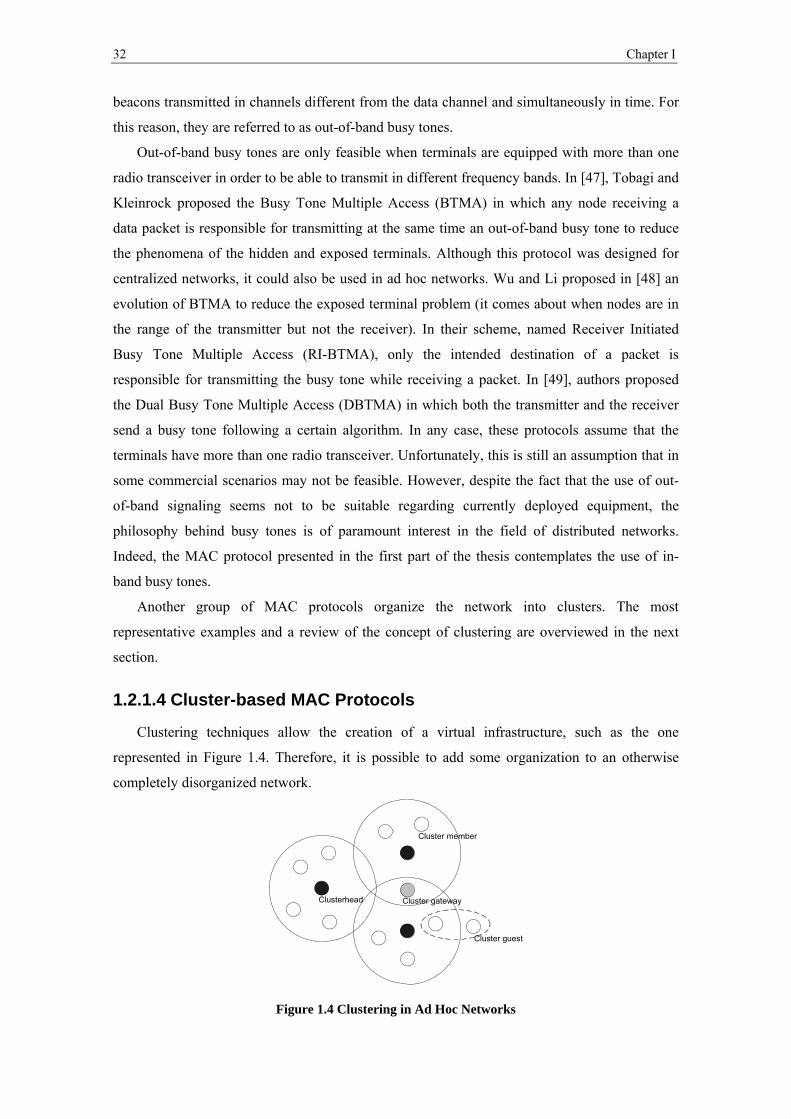
Chapter I 32
beacons transmitted in channels different from the data channel and simultaneously in time. For
this reason, they are referred to as out-of-band busy tones.
Out-of-band busy tones are only feasible when terminals are equipped with more than one
radio transceiver in order to be able to transmit in different frequency bands. In [47], Tobagi and
Kleinrock proposed the Busy Tone Multiple Access (BTMA) in which any node receiving a
data packet is responsible for transmitting at the same time an out-of-band busy tone to reduce
the phenomena of the hidden and exposed terminals. Although this protocol was designed for
centralized networks, it could also be used in ad hoc networks. Wu and Li proposed in [48] an
evolution of BTMA to reduce the exposed terminal problem (it comes about when nodes are in
the range of the transmitter but not the receiver). In their scheme, named Receiver Initiated
Busy Tone Multiple Access (RI-BTMA), only the intended destination of a packet is
responsible for transmitting the busy tone while receiving a packet. In [49], authors proposed
the Dual Busy Tone Multiple Access (DBTMA) in which both the transmitter and the receiver
send a busy tone following a certain algorithm. In any case, these protocols assume that the
terminals have more than one radio transceiver. Unfortunately, this is still an assumption that in
some commercial scenarios may not be feasible. However, despite the fact that the use of out-
of-band signaling seems not to be suitable regarding currently deployed equipment, the
philosophy behind busy tones is of paramount interest in the field of distributed networks.
Indeed, the MAC protocol presented in the first part of the thesis contemplates the use of in-
band busy tones.
Another group of MAC protocols organize the network into clusters. The most
representative examples and a review of the concept of clustering are overviewed in the next
section.
1.2.1.4 Cluster-based MAC Protocols
Clustering techniques allow the creation of a virtual infrastructure, such as the one
represented in Figure 1.4. Therefore, it is possible to add some organization to an otherwise
completely disorganized network.
Clusterhead
Cluster member
Cluster gateway
Cluster guest
Figure 1.4 Clustering in Ad Hoc Networks
Introduction
33
As can be seen in this figure, within every group or cluster, each node can play different
roles depending on either its position or function. A node might be set to clusterhead if it is the
principal node in the cluster and is governing its one-hop neighborhood or to cluster member if
it is connected to a clusterhead. Furthermore, a node may act as a clustergateway, if it is
connected to more than one clusterhead at the same time and therefore it is a potential relay for
the inter-cluster communication, or as a clusterguest, if it is able to connect to a cluster member
but not to a clusterhead.
Among the benefits of clustering, the most important are:
1) Increase of the spatial reuse of the radio resources to enhance the system capacity.
2) Reduction of the routing protocol information. The intra-cluster routing can be managed
by the cluster members, whereas inter-cluster routing is handled only among
clusterheads.
3) Reduction of the topological update information. Since nodes forming a cluster can be
considered as one unit, this cluster-oriented approach minimizes the topological
information exchange throughout the ad hoc network. When a node moves from one
cluster to another, only those nodes included in the involved clusters have to be notified,
instead of the whole network.
4) Applicability of previously designed and optimized radio resource management
algorithms for cellular-oriented wireless networks within each cluster, hence
maximizing the use of the resources and minimizing the occurrence of collisions, in the
case of the MAC protocols.
5) In the case of selecting special nodes with extra tasks, i.e., clusterheads, clustering eases
the provision of QoS, since centralized polling can be applied and synchronization can
be established.
Assuming that all the clusters operate with a single common channel, the spatial reuse of
clustering is strongly determined by the size of the clusters, which is a key design parameter.
Small clusters can lead to a better spatial reuse; however, the end to end delay can be
dramatically increased due to the long paths in terms of number of hops existing between pairs
of nodes. This delay can be reduced with big clusters, however, in this case, the spatial reuse is
diminished, and moreover, the interference range is increased. Therefore, a tradeoff has to be
managed when designing the size of the clusters, and hence the spatial reuse factor of the
clustering scheme. It is important to note that, in general, most nodes forming a mobile ad hoc
network have a finite battery, so the cluster-size design might be constrained by the power
consumption requirements of the nodes. Big clusters imply higher transmission power and,
therefore, higher power consumption. Moreover, as this power consumption does not grow
linearly with the increase of the distance, the total energy cost of the transmission is also
affected by the increase of the cluster size.
Chapter I 34
Unfortunately, the process of clustering has a certain cost. The set up and maintenance of a
clustered architecture could imply a partial loss of the available resources. This may be an
important drawback that has to be kept in mind when considering clustering. The loss of
resources could be caused by three possible reasons:
1) The need for the explicit exchange of clustering information.
2) The time required to execute the clustering mechanisms.
3) The costly process of re-clustering as the mobility of the network may lead to frequent
changes in the topology and connectivity among the terminals.
Another potential drawback of clustering arises when applying some kind of clusterhead
centralization. Some researchers assure that although some nodes should be selected as
clusterheads, they should not take extra tasks assignment in order to avoid becoming the
bottleneck of the network. Besides, such scheme would not be scalable when large-size
networks are considered. On the other hand, other researchers promote assigning extra tasks to
clusterheads in order to create a virtual backbone.
Therefore, some tradeoffs have to be managed between the benefits of clustering and its
associated costs.
So far, lots of clustering algorithms and cluster-based MAC protocols have been proposed
in the literature; the ones in [50]-[63], that we review next, are only a few. A complete survey
and classification of other clustering schemes can be found in [64]. All of these strategies differ
in the dynamic mechanisms used to set up the network clusters and to define the roles of the
stations.
For example, in [50], an out-of-band control channel is devoted to the exchange of “hello”
messages among mobile terminals in order to set the clusterhead and the cluster members of
each cluster. The key of the protocol resides in the specific MAC protocol, called Three Phase
Multiple Access (TPMA), which has been designed to transmit the control messages with which
the cluster algorithm is executed. Also taking advantage of out-of-band signaling, in [51] the
control channel is divided into three time slots reserved for a mechanism based on two busy
tones (primary and secondary) to avoid inter-cell interference, i.e., interference between
neighboring clusters. In [52], the (, t) cluster strategy is presented; in this case the network is
partitioned into clusters of nodes that are mutually reachable along cluster internal paths that are
expected to be available with a probability for a period of time t. In [53] the Multimedia
support for Mobile Wireless Networks (MMWN) is outlined, focusing on a clustering
mechanism which classifies nodes into switches and endpoints while defining a dynamic multi-
level cluster architecture, i.e., lower level clusters group themselves to form higher-level
clusters. The clustering association is based on the link quality between endpoints and switches
and the quality-of-service requirements of the endpoints. This approach could be considered as a
first step into the cross-layer design for clustering. Also focused on multimedia support in ad
Introduction
35
hoc networks, the possibility of making independent the operation of the different clusters is
proposed in [54], where the network is organized into non-overlapping clusters relying on a
code-division access scheme. Although most of the proposals for clustering are based on the
concept of clusterheads that act as local coordinators within each cluster, this proposal
eliminates the requirement for a clusterhead altogether. Adopting a fully distributed approach
for cluster formation, potential bottlenecks are avoided. Combining time division and code
division multiplexing, in [55] a multi-hop architecture is proposed. In this proposal, clusterheads
act as local coordinators to resolve channel scheduling, perform power measurements and
control, maintain time division frame synchronization, and enhance spatial reuse of time slots
and codes. The election of the clusterheads can be based on two different criteria; i) the lowest-
ID node in a neighborhood, or ii) the node with higher degree, that is, with highest connectivity.
In [56], the Mobile Point Coordinator (MPC) protocol is presented in combination with the PCF
of the IEEE 802.11 Standard to provide some degree of QoS over distributed networks. In MPC,
stations maintain a list of potential clusterheads and they exchange “hello” messages to decide,
using an agreed-upon policy, which is the virtual infrastructure. Although the general approach
of MPC is very interesting as a methodology to extend the operation of an infrastructure-based
MAC protocol to distributed networks, authors propose an over-engineered exchange of power-
dynamic mini-pulses in the clustering phases that may compromise its applicability in actual
hardware.
A topic that has given rise to many cluster-based MAC protocols is vehicular
communications, as reported in [57] and [58]. Most of the proposals in this field assume that
different channels can be used to separate data from control, or to avoid inter-cluster
interference. Therefore, they assume that cars are equipped with more than one radio
transceiver, which is a reasonable assumption for that specific application. Unfortunately, this is
not a realistic assumption in many other applications, such as disaster management situations for
example, where mobile users might be equipped with simple and small devices.
Some other cluster-based MAC protocols have been designed based on CDMA techniques
[59]-[61]. In these proposals, nodes are clustered into different groups in which they can
communicate by using a common spreading code. For example, [59] and [60] present MAC
approaches in which clusters exploit the diversity attained by Direct Sequence Spread Spectrum
(DSSS). In the context of Bluetooth systems, for example, dynamic master-slave architecture is
adopted where clusters use different hopping sequences by exploiting a Frequency Hopping
Spread Spectrum (FHSS) access technique [61]. The challenge in these cases is the problem of
assigning a different code to each cluster in order to avoid intercluster interference, as reported
in [62] and [63]. This is related to a classic graph coloring problem.
In this thesis, the aim is to propose a spontaneous and passive cluster-based MAC protocol
which runs with a single transceiver. The main motivation for this last characteristic is that
Chapter I 36
current standards and devices for WLAN do not contemplate the use of several radio
transceivers. In addition, the proposed clustering mechanism does not require any pre-
configuration of the network, nor coding planning or slot pre-allocation, but it is designed on the
same basis as the nature of the ad hoc networks which are established to satisfy a spontaneous
and dynamic need. To the best of our knowledge, this approach is novel in the field.
With this section, the overview of the state of the art regarding MAC protocols is
completed. As aforementioned, several interesting proposals have been not included in this
summary since a complete thesis dissertation could be written on the topic. The most relevant
proposals have been presented and an extensive bibliographic reference list has been provided
so that the interested reader can go into more detail.
In the next section, an overview of the analytical models that can be found in the literature
regarding the theoretical performance analysis of MAC protocols for ad hoc networks is
presented.
1.2.2 Analytical Models for MAC Protocols in Ad hoc Networks
The theoretical understanding of wireless ad hoc networks can help in designing optimal
communication protocols by defining estimates and bounds of the performance. Without this
understanding, designers have no direction to follow and the limits of the network capacity are
unknown. Unfortunately, the complexity and degrees of freedom of ad hoc networks turn the
topic into a great challenge that grows exponentially in complexity with the number of stations
in the network [65]. Despite these difficulties, some efforts have been done to model wireless
networks as described hereafter.
Some work has been focused on finding fundamental upper bounds on the capacity of a
multihop distributed network from an information theoretic point of view. Seminal findings by
Gupta and Kumar in [66] set the relationship between the per-node throughput (T) and the
number of nodes n as 1/T n . Subsequent works have studied the network capacity from
different points of view. For example, the increased capacity attained with user mobility is
assessed in [67]. A framework to derive the capacity of CSMA-based ad hoc networks handling
delay sensitive traffic is presented in [68]. Authors in both [69] and [70] elaborate on the
capacity of ad hoc networks exploiting the capabilities of directional antennas, while Toumpis
and Goldsmith presented in [71] a framework to derive the capacity regions of ad hoc networks.
From the MAC point of view, another line of work has been focused on trying to derive
expressions of throughput and delay for specific MAC protocols for single-hop networks (where
all nodes are in the transmission range of each other) in saturation conditions. This is the
example of the Bianchi’s IEEE 802.11 model presented in [72], based on the seminal approach
of Abramson when modeling the ALOHA MAC protocol in [73] and [74], or of Kleinrock and
Tobagi when modeling CSMA in [8] and [47]. All these models are characterized by some ideal
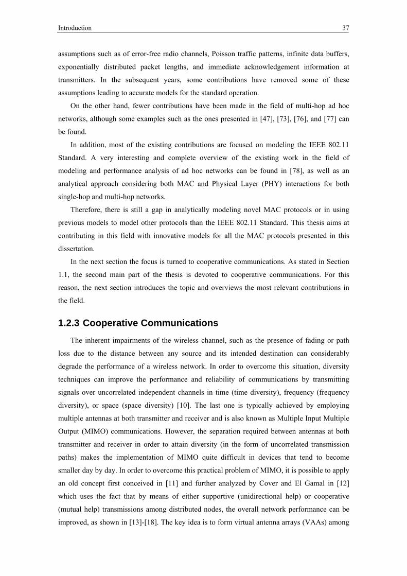
Introduction
37
assumptions such as of error-free radio channels, Poisson traffic patterns, infinite data buffers,
exponentially distributed packet lengths, and immediate acknowledgement information at
transmitters. In the subsequent years, some contributions have removed some of these
assumptions leading to accurate models for the standard operation.
On the other hand, fewer contributions have been made in the field of multi-hop ad hoc
networks, although some examples such as the ones presented in [47], [73], [76], and [77] can
be found.
In addition, most of the existing contributions are focused on modeling the IEEE 802.11
Standard. A very interesting and complete overview of the existing work in the field of
modeling and performance analysis of ad hoc networks can be found in [78], as well as an
analytical approach considering both MAC and Physical Layer (PHY) interactions for both
single-hop and multi-hop networks.
Therefore, there is still a gap in analytically modeling novel MAC protocols or in using
previous models to model other protocols than the IEEE 802.11 Standard. This thesis aims at
contributing in this field with innovative models for all the MAC protocols presented in this
dissertation.
In the next section the focus is turned to cooperative communications. As stated in Section
1.1, the second main part of the thesis is devoted to cooperative communications. For this
reason, the next section introduces the topic and overviews the most relevant contributions in
the field.
1.2.3 Cooperative Communications
The inherent impairments of the wireless channel, such as the presence of fading or path
loss due to the distance between any source and its intended destination can considerably
degrade the performance of a wireless network. In order to overcome this situation, diversity
techniques can improve the performance and reliability of communications by transmitting
signals over uncorrelated independent channels in time (time diversity), frequency (frequency
diversity), or space (space diversity) [10]. The last one is typically achieved by employing
multiple antennas at both transmitter and receiver and is also known as Multiple Input Multiple
Output (MIMO) communications. However, the separation required between antennas at both
transmitter and receiver in order to attain diversity (in the form of uncorrelated transmission
paths) makes the implementation of MIMO quite difficult in devices that tend to become
smaller day by day. In order to overcome this practical problem of MIMO, it is possible to apply
an old concept first conceived in [11] and further analyzed by Cover and El Gamal in [12]
which uses the fact that by means of either supportive (unidirectional help) or cooperative
(mutual help) transmissions among distributed nodes, the overall network performance can be
improved, as shown in [13]-[18]. The key idea is to form virtual antenna arrays (VAAs) among
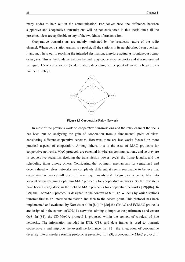
Chapter I 38
many nodes to help out in the communication. For convenience, the difference between
supportive and cooperative transmissions will be not considered in this thesis since all the
presented ideas are applicable to any of the two kinds of transmission.
Cooperative transmissions are mainly motivated by the broadcast nature of the radio
channel. Whenever a station transmits a packet, all the stations in its neighborhood can overhear
it and may help out in reaching the intended destination, therefore acting as spontaneous relays
or helpers. This is the fundamental idea behind relay cooperative networks and it is represented
in Figure 1.5 where a source (or destination, depending on the point of view) is helped by a
number of relays.
Source Dest.
Relay
Relay
Relay
Relay
Figure 1.5 Cooperative Relay Network
In most of the previous work on cooperative transmissions and the relay channel the focus
has been put on analyzing the gain of cooperation from a fundamental point of view,
considering different cooperative schemes. However, there are less works focused on more
practical aspects of cooperation. Among others, this is the case of MAC protocols for
cooperative networks. MAC protocols are essential in wireless communications, and so they are
in cooperative scenarios, deciding the transmission power levels, the frame lengths, and the
scheduling times among others. Considering that optimum mechanisms for centralized and
decentralized wireless networks are completely different, it seems reasonable to believe that
cooperative networks will pose different requirements and design parameters to take into
account when designing optimum MAC protocols for cooperative networks. So far, few steps
have been already done in the field of MAC protocols for cooperative networks [79]-[84]. In
[79] the CoopMAC protocol is designed in the context of 802.11b WLANs by which stations
transmit first to an intermediate station and then to the access point. This protocol has been
implemented and evaluated by Korakis et al. in [84]. In [80] the CMAC and FCMAC protocols
are designed in the context of 802.11e networks, aiming to improve the performance and ensure
QoS. In [81], the CD-MACA protocol is proposed within the context of wireless ad hoc
networks. The information included in RTS, CTS, and data frames is used to transmit
cooperatively and improve the overall performance. In [82], the integration of cooperative
diversity into a wireless routing protocol is presented. In [83], a cooperative MAC protocol is
Introduction
39
presented within the context of a centralized mesh network formed by the access point, regular
stations and fixed wireless routers (relays), in which empty TDMA slots are used for
cooperative relaying performed by the relay infrastructure.
Despite these first steps, there is still a long way ahead in developing novel protocols and
analyzing the feasibility of reutilizing already well known MAC protocols to fulfill the
requirements of cooperative relay networks. This is the main motivation for the contribution
presented in the second part of the thesis.
1.3 Main Contributions and Structure of the Thesis
Taking into account the background presented in the previous section, the main
contributions of the thesis are outlined in this section.
As aforementioned, the thesis is comprised of three parts: a preliminary background part
comprised of this first chapter and Chapter II, and two other interconnected main parts with the
key contributions of the thesis.
The first main part of the thesis is comprised of Chapters III and IV. These chapters are
focused on the design and performance analysis and evaluation of two novel high-performance
MAC protocols for ad hoc networks. More precisely, the main contributions of the first main
part of the thesis are:
1) Design of the Distributed Queueing MAC protocol for Ad Hoc Networks (DQMAN),
which is an extension and adaptation of the near-optimum DQCA protocol in order to
operate in ad hoc networks. The protocol integrates a modified version of DQCA with a
passive-based spontaneous and temporary master-slave clustering algorithm.
2) Analytical modeling of the performance of DQMAN in both saturation and non-
saturation conditions in single-hop networks.
3) Proposal of modifications of the protocol to achieve performance enhancements under
heavy traffic conditions.
4) Performance evaluation of DQMAN in multi-hop environments.
5) Design of the Distributed Point Coordination Function (DPCF), which constitutes an
extension and adaptation of the PCF of the IEEE 802.11 for operation in ad hoc
networks. This protocol exemplifies that the rationale of the extension of DQCA to
DQMAN can be, indeed, applied to any other infrastructure-based MAC protocol.
6) Performance evaluation of DPCF based on computer simulation.
The second main part of the thesis is focused on C-ARQ schemes and is confined to
Chapter V of this dissertation. The main contributions of the second main part of the thesis
are:
1) Design, analysis, and performance evaluation of the DQMAN for C-ARQ protocol,
named DQCOOP.
Chapter I 40
2) Design, analysis, and performance evaluation of PRCSMA, presented as an adaptation
of the IEEE 802.11 Standard to operate with C-ARQ schemes.
3) Comprehensive comparison of the performance of a network using non-traditional ARQ
with respect to three different C-ARQ schemes; one with ideal scheduling among the
relays, and two others with DQCOOP and PRCSMA executed at the MAC layer.
4) Analysis and performance evaluation of a rooftop Access Point (AP) network
considering non-cooperative ARQ and C-ARQ with either DQCOOP or PRCSMA at
the MAC layer.
In the process of preparing this thesis, a custom-made C++ simulator, called MACSWIN
has been developed. This simulator has made possible the validation of the accuracy of the
theoretical models developed within the thesis. In addition, MACSWIN has been also used to
evaluate the performance of the different considered communication networks under some
assumptions that the theoretical models cannot cover. A comprehensive description of
MACSWIN, together with a description of the theoretical framework of the thesis, is presented
in Chapter II.
Finally, Chapter VI concludes the thesis, summarizes the main findings, and outlines future
lines of research.
In the next section, the list of publications in international journals and conferences which
help in the dissemination of the ideas exposed in this thesis is presented.
1.4 Dissemination
The contents of the first part of the thesis have been presented in one journal:
J. Alonso-Zárate, E. Kartsakli, C. Skianis, C. Verikoukis, and L. Alonso, “Saturation
Throughput Analysis of a Cluster-Based Medium Access Control Protocol for Single-
hop Ad Hoc Wireless Networks,” Simulation: Trans. of the Society for Modeling and
Simulation International, vol. 84, no.12, pp. 619-633, Dec. 2008.
and eight international conferences:
C. Crespo, J. Alonso-Zárate, C. Verikoukis, and L. Alonso, “Distributed Point
Coordination Function for Wireless Ad Hoc Networks,” in Proc. of the IEEE Vehicular
Technology Conference (VTC Spring 2009), Barcelona (Spain), 2009.
J. Alonso-Zárate, E. Kartsakli, C. Verikoukis, and L. Alonso, “Saturation Throughput
Analysis of a Passive Cluster-based Medium Access Control Protocol for Ad Hoc
Wireless Networks,” in Proc. of the IEEE International Conference on Communications
(ICC’08), Beijing (China), May 2008.
J. Alonso-Zárate, E. Kartsakli, C. Verikoukis, and L. Alonso, “Performance
Enhancement of DQMAN-based Wireless Ad Hoc Networks in Multi-Hop Scenarios,”
Introduction
41
in Proc. of the IEEE International Symposium on Wireless Pervasive Computing
(ISWPC’08), Santorini (Greece), May 2008.
J. Alonso-Zárate, E. Kartsakli, A. Cateura, C. Verikoukis, and L. Alonso, “Enhanced
Operation of DQMAN based Wireless Ad Hoc Networks,” in Proc. of the IEEE
International Symposium on Wireless Systems (ISWCS’07), Trondheim (Norway), Oct.
2007.
Jesús Alonso, Christos Verikoukis, and Luis Alonso, “Fairness Enhancement in a Self-
Configuring Cluster-Based Wireless Ad Hoc Network,” in Proc. of the International
Conference on Wireless Personal Multimedia Communications (WPMC’05), Aalborg
(Denmark), Sep. 2005.
Jesús Alonso, Christos Verikoukis, and Luis Alonso, “Performance Analysis of a
Distributed Queueing MAC Protocol for Ad Hoc networks With Different Mobility
Conditions,” in Proc. of the International Conference on Mobile and Wireless
Communications Networks (MWCN’05), Marrakech (Morocco), Sep. 2005.
Jesús Alonso and Luis Alonso, “A Novel MAC Protocol For Dynamic AD HOC
Wireless Networks With Dynamic Self-Configurable Master-Slave Architecture,” in
Proc. of the IEEE Symposium on Personal, Indoor, and Mobile Radio Communications
(PIMRC’04), Barcelona (Spain), Sep. 2004.
Jesús Alonso and Luis Alonso, “Dynamic Self-Constructing Master-Slave Architecture
for AD HOC Wireless Networks With a Distributed MAC Scheme,” in Proc. of the
IEEE Vehicular Technology Conference (VTC Fall 2004), Los Angeles (US), Sep.
2004.
The contents of the second part of the thesis have been presented in one journal:
J. Alonso-Zárate, E. Kartsakli, C. Verikoukis, and L. Alonso, “Persistent RCSMA: A
MAC Protocol for a Distributed Cooperative ARQ Scheme in Wireless Networks,”
EURASIP Journal on Advanced Signal Processing, Special Issue on Wireless
Cooperative Networks, vol. 2008, article ID 817401, pp. 13, May 2008.
and five international conferences:
J. Alonso-Zárate, E. Kartsakli, Ch. Verikoukis, and L. Alonso, “Throughput Analysis of
a Medium Access Control Protocol for a Distributed Cooperative ARQ Scheme in
Wireless Networks,” in Proc. of the IEEE GLOBECOM 2008, New Orleans (USA),
Dec. 2008.
J. Alonso-Zárate, E. Kartsakli, Ch. Verikoukis, and L. Alonso, “A Novel Near-
Optimum Medium Access Control Protocol for a Distributed Cooperative ARQ Scheme
in Wireless Networks,” in Proc. of the IEEE Symposium on Personal, Indoor, and
Mobile Radio Communications (PIMRC), Cannes (France), Sep. 2008.
Chapter I 42
J. Alonso-Zárate, P. Giotis, E. Kartsakli, C. Verikoukis, and L. Alonso, “Performance
Evaluation of a Medium Access Control Protocol for Distributed Cooperative ARQ
schemes in Wireless Networks,” in Proc. of the ICT Mobile Summit, Stockholm
(Sweden), Jun. 2008.
J. Gómez, J. Alonso-Zárate, C. Verikoukis, A. Pérez-Neira, and L. Alonso,
“Cooperation On Demand Protocols for Wireless Networks,” in Proc. of the IEEE
Symposium on Personal, Indoor, and Mobile Radio Communications (PIMRC’07),
Athens (Greece), Sep. 2007.
J. Alonso-Zárate, J. Gómez, C. Verikoukis, L. Alonso, and A. Pérez-Neira,
“Performance Evaluation of a Cooperative Scheme for Wireless Networks,” in Proc. of
the IEEE Symposium on Personal, Indoor, and Mobile Radio Communications
(PIMRC’06), Helsinki (Finland), Sep. 2006.
1.5 Other Research Contributions
Besides the main contributions of this thesis outlined in the previous section, a number of
other research works have been carried out while this thesis was being written.
This thesis deals with DQMAN, which constitutes the adaptation and extension of the
infrastructure-based DQCA protocol to operate over distributed ad hoc networks. In the process
of designing DQMAN, some improvements in the performance of the DQCA have been also
conducted. The performance improvement that can be attained by considering cross-layer
design in the MAC protocol operation has been analyzed and studied and the most relevant
results have been published in three journals:
E. Kartsakli, J. Alonso-Zárate, L. Alonso, and C. Verikoukis, “Cross-Layer Scheduling
with QoS Support over a Distributed Queuing MAC for Wireless LANs," accepted for
publication in ACM/Springer Mobile Networks and Applications Special Issue on
"Recent Advances in IEEE 802.11 WLANs: Protocols, Solutions, and Future
Directions”.
E. Kartsakli, A. Cateura, J. Alonso-Zárate, Ch. Verikoukis, and L. Alonso, “Cross-
Layer Enhancement for WLAN Systems with Heterogeneous Traffic based on DQCA,”
IEEE Communications Magazine Radio Communications Series, vol. 46, no. 6, pp. 60-
66, Jun. 2008.
J. Alonso-Zárate, E. Kartsakli, A. Cateura, C. Verikoukis, and L. Alonso, “A Near-
Optimum Cross-Layered Distributed Queueing Protocol for Wireless LAN,” IEEE
Wireless Communication Magazine, Special Issue on MAC protocols for WLAN, vol.
15, no. 1, pp. 48-55, Feb. 2008.
and three international conferences:
Introduction
43
E. Kartsakli, A. Cateura, J. Alonso-Zárate, Ch. V. Verikoukis, and L. Alonso, “Cross-
Layer Enhancement for WLAN Systems with Heterogeneous Traffic Based on DQCA,”
in Proc. of the IEEE International Conference on Communications 2007 (ICC’07),
Glasgow (Scotland), Jun. 2007.
E. Kartsakli, A. Cateura, J. Alonso-Zárate, C. Verikoukis, and L. Alonso,
“Opportunistic Scheduling using an Enhanced Channel State Information Update
Scheme for WLAN Systems with DQCA,” in Proc. of the IEEE Vehicular Technology
Conference Spring (VTC Spring 2007), Dublin (Ireland), 2007.
C. Verikoukis, J. Alonso-Zárate, A. Cateura, E. Kartsakli, and L. Alonso, “Cross-Layer
Enhancement for WLAN Systems based on a Distributed Queueing MAC Protocol,” in
Proc. of the IEEE Vehicular Technology Conference Spring (VTC Spring 2006),
Melbourne (Australia) 2006.
In addition, during the whole development of this thesis, a book chapter devoted to
contention-based collision-resolution MAC protocols has also been published:
E. Kartsakli, J. Alonso-Zárate, A. Cateura, Ch. Verikoukis, and L. Alonso, contribution
to the book “Medium Access Control in Wireless Networks,” published by Nova
Science Publishers Inc, ISBN-1-60021-944-6. with the chapter entitled “Contention-
Based Collision-Resolution Medium Access Control Algorithms,” pp. 15-97, Feb. 2008.
Recently, in January 2009, another book chapter entitled “Cross-Layer Scheduling with
QoS Support over a Near-Optimum Distributed Queueing Protocol for Wireless LAN” has been
accepted to be published within the book “Wireless Network Traffic and Quality of Service
Support: Trends and Standards,” published by IGI Publishing.
Although not directly related with the contents of the thesis, it is also worth mentioning two
other contributions published in two national conferences:
J. Alonso-Zárate, I. Ramos, E. Kartsakli, C. Verikoukis, and L. Alonso, “Evaluación de
algoritmos Cross-Layer para la Optimización de Comunicaciones Inalámbricas en modo
Ad Hoc,” in Proc. of the Jornadas Telecom I+D 2006, Madrid (Spain) Nov. 2006.
J. Alonso-Zárate, A. Cateura, E. Kartsakli, C. Verikoukis, and L. Alonso, “Estudio del
rendimiento de protocolos de acceso para redes inalámbricas con antenas
direccionales,” in Proc. of the XXI Simpósium Nacional de la Unión Científica
Internacional de Radio de 2006, Oviedo (Spain), Sep. 2006.
1.6 References
[1] The 16th WWRF Meeting, 26-28 April, 2006, Shanghai, China, http://www.wireless-
world-research.org/.
[2] C. E. Perkins, “Ad Hoc Networking,” Pearson Professional, 2000.
Chapter I 44
[3] A. Chandra, V. Gummallak, and J. O. Limb, “Wireless Access Control Protocols,”
IEEE Communications Surveys & Tutorials, Second Quarter 2000.
[4] R. Jurdak, C. Videira Lopes, and P. Baldi, “A Survey, Classification and Comparative
Analysis of Medium Access Control Protocols for Ad Hoc Networks,” IEEE
Communications Surveys & Tutorials, First Quarter 2004.
[5] S. Kumar, V. S. Raghavan, and J. Deng, “Medium Access Control protocols for ad hoc
wireless networks: A survey,” Ad Hoc Networks, Elsevier, 2004.
[6] H. Zai, J. Wang, X. Chen, and Y. Fang, “Medium Access Control in mobile ad hoc
networks: challenges and solutions,” Wireless Communications and Mobile Computing,
vol. 6, pp. 151-170, John Wiley & Sons, 2006.
[7] J. Alonso-Zárate, E. Kartsakli, A. Cateura, C. Verikoukis, and L. Alonso, “A Near-
Optimum Cross-Layered Distributed Queueing Protocol for Wireless LAN,” IEEE
Wireless Communication Magazine, Special Issue on MAC protocols for WLAN, vol.
15, no. 1, pp. 48-55, Feb. 2008.
[8] L. Kleinrock and F. A. Tobagi, “Packet Switching in radio channels: Part I – Carrier
Sense Multiple-Access Models and their Throughput-Delay Characteristics,” IEEE
Trans. on Communications, vol. 23, pp. 1400-1416, Dec. 1975.
[9] IEEE, Part 11: Wireless LAN Medium Access Control (MAC) and Physical Layer
(PHY) Specifications, IEEE Std. 802.-11-99, Aug. 1999.
[10] A. Nosratinia, T. E. Hunter, and A. Hedayat, “Cooperative Communications in Wireless
Networks,” IEEE Communications Magazine, vol. 42, no. 10, pp. 74-80, Oct. 2004.
[11] E. Van der Meulen, “Three-terminal communication channels,” Bell. Syst. Tech.
Journal, vol. 27, pp. 379-423, Jul.-Oct. 1971.
[12] T. M. Cover and A. E. Gamal, “Capacity Theorems for the Relay Channel,” IEEE
Trans. on Information Theory, vol. 25, no. 5, p. 572, Sep. 1979.
[13] A. Sendonaris, E. Erkip, and B. Aazhang, “Increasing Uplink Capacity via Station
Cooperation Diversity,” in Proc. of the IEEE International Symposium on Information
Theory (ISIT’98), Cambridge, MA, p.156, Aug. 1998.
[14] A. Sendonaris, E. Erkip, and B. Aazhang, “Station Cooperation Diversity-Part I: System
Description,” IEEE Trans. on Communications, vol. 51, no. 11, pp. 1927-1938, Nov.
2003.
[15] A. Sendonaris, E. Erkip, and B. Aazhang, “Station Cooperation Diversity-Part II:
Implementation Aspects and Performance Analysis,” IEEE Trans. on Communications,
vol. 51, no. 11, pp. 1939-1948, Nov. 2003.
Introduction
45
[16] M. Dohler, Virtual Antenna Arrays, Ph. D. Thesis Dissertation, King’s College London,
2003.
[17] J. N. Laneman, D. N. C. Tse, and G. W. Wornell, “Cooperative Diversity in Wireless
Networks: Efficient Protocols and Outage Behavior,” IEEE Trans. on Information
Theory, vol. 50, no. 12, Dec. 2004.
[18] J. N. Laneman and G. W. Wornell, “Distributed Space-Time-Coded Protocols for
Exploiting Cooperative Diversity in Wireless Networks,” IEEE Trans. on Information
Theory, vol. 49, no. 10, pp. 2415-25, Oct. 2003.
[19] M. Dianati, X. Ling, K. Naik, and X. Shen, “A Node-Cooperative ARQ Scheme for
Wireless Ad Hoc Networks,” IEEE Trans. on Vehicular Technology, vol. 55, no. 3, pp.
1032-1044, May 2006.
[20] M. Zorzi, R. R. Rao, and L. B. Milstein, “ARQ error control for fading mobile radio
channels,” IEEE Trans. on Vehicular Technology, vol. 46, no. 2, pp. 445-455, May
1997.
[21] E. Zimmermann, P. Herhold, and G. Fettweis, “The Impact of Cooperation on
Diversity-Exploting Protocols,” in Proc. of the 59th IEEE Vehicular Technology
Conference 2004.
[22] E. Zimmermann, P. Herhold, and G. Fettweis, “On the Performance of Cooperative
Relaying Protocols in Wireless Networks,” European Trans. on Telecommunications,
vol. 16, no. 1, pp. 5-16, Jan. 2005.
[23] P. Gupta, I. Cerruti, and A. Fumagalli, “Three Transmission Scheduling Policies for a
Cooperative ARQ Protocol in Radio Networks,” in Proc. of the WNCG Conference,
Austin, Oct.2004.
[24] I. Cerruti, A. Fumagalli, and P. Gupta, “Delay Model of Single-Relay Cooperative ARQ
Protocols in Slotted Radio Networks Poisson Frames Arrivals,” IEEE/ACM Trans. on
Networking, vol. 16, no. 2, Apr. 2008.
[25] J. Morillo-Pozo, J. García-Vidal, and A. I. Pérez-Neira, “Collaborative ARQ in
Wireless Energy-Constrained Networks,” in Proc. of the 2005 Joint Workshop on
Foundations of Mobile Computing 2005 (DIAL-POM’05).
[26] S. Biswas and R. Morris, "ExOR: Opportunistic Multi-hop Routing for Wireless
Networks,” in Proc. of the SIGCOMM '05. New York, NY, USA, 2005, pp. 133-144.
[27] P. Larsson and N. Johansson, "Multistation Diversity Forwarding in Multihop Packet
Radio Networks,” in Proc. of the IEEE Wireless Communications and Networking
Conference 2005, pp. 2188-2194.
Chapter I 46
[28] J. García-Vidal, “Addressing and Forwarding in Cooperative Wireless Networks,”
UPC-DAC-RR-XCSD-2005-8, Dec. 2005.
[29] H. Wu and Y. Pan, “Medium Access Control in Wireless Networks,” NOVA Science
Publishers, 2008.
[30] J. A. Stine, “Exploiting Smart Antennas in Wireless Mesh Networks Using Contention
Access,” IEEE Wireless Communications, Apr. 2006.
[31] R. R. Choudhury, X. Yang, R. Ramanathan, and N. H. Vaydia, “On Designing MAC
Protocols for Wireless Networks Using Directional Antennas,” IEEE Trans. on Mobile
Computing, vol. 5, no. 5, May 2006.
[32] P. Karn, “MACA: A New Channel Access Protocol for Packet Radio,” ARRL/CRRL
Amateur Radio 9th Comp. Net. Conf. 1990, pp. 134-40.
[33] V. Bharghavan et al., “MACAW: A Media Access Protocol for Wireless LANs,” in
Proc. of the ACM SIGCOMM ’94, pp. 212-25, 1994.
[34] C. L. Fullmer and J. J. Garcia-Luna-Aceves, “Floor Acquisition Multiple Access
(FAMA) for packet radio networks,” in Proc. of the Conf. Applications, Tech.,
Architectures and Protocols for Comp. Comm. (SIGCOMM), 1995, pp. 262-73.
[35] G. Bianchi, L. Fratta, and M. Oliveri, “Performance Evaluation and Enhancement of the
CSMA/CA MAC protocol for 802.11 Wireless LAN’s,” in Proc. of the IEEE PIMRC
1996, Taipei, Taiwan, pp. 392-296, Oct., 1996.
[36] J. Weinmiller, M. Schläger, A. Festag, and A. Wolisz, “Performance Study of Access
Control in Wireless LANs-IEEE 802.11 DFWMAC and ETSI RES 10 HIPERLAN,”
Mobile Networks Appl., vol. 2, pp. 55-67, 1997.
[37] F. Cali, M. Conti, and E. Gregori, “Dynamic Tuning of the IEEE 802.11 Protocol to
Achieve a Theoretical Throughput Limit,” IEEE/ACM Transaction on Networking, vol.
8, no. 6, pp. 785-799, Dec. 2006.
[38] S. Agarwal, S. Krishnamurthy, R. H. Katz, and S. D. Kao, “Distributed power control in
ad hoc wireless networks,” in Proc. of the IEEE PIMRC, 2001.
[39] E. S. Jung and N. H. Vaydia, “A Power Control MAC protocol for ad hoc networks,” in
Proc. of the ACM Mobicom, Atlanta, GA, pp. 36-47, Sep. 2002.
[40] Z. Tang and J. J. Garcia-Luna-Aceves, “A protocol for topology-dependant
transmission scheduling in wireless networks,” in Proc. of the IEEE WCNC, vol. 3,
New Orleans, LA, pp. 1333-1337, Sep. 1999.
[41] S. Toumpis and A. Goldsmith, “Performance, optimization, and cross-layer design of
media access control protocols for wireless ad hoc networks,” in Proc. of the IEEE ICC,
Anchorage, AK, pp. 2234-2240, May 2003.
Introduction
47
[42] D. J. Goodman, R. A. Valenzuela, K. T. Gayliard, and B. Ramamurthi, “Packet
Reservation Multiple Access for Local Wireless Networks,” IEEE Trans. on
Communications, vol. 37, no. 8, Aug. 1989.
[43] I. Chlamtac, A. Faragó, A. D. Myers, V. R. Syrotiuk, and G. V. Záruba, “ADAPT: A
dynamically self-adjusting media access control protocol for ad hoc networks,” in Proc.
of the GLOBECOM, pp. 11-15, Dec. 1999.
[44] A. Rhee, M. Warrier, and J. Min, “ZMAC: A hybrid MAC for wireless sensor
networks,” in Proc. of Sensys 2005, San Diego, California.
[45] M. Shakir, I. Ahmed, P. Mugen, and W. Wang, “Cluster Organization based Design of
Hybrid MAC Protocol in Wireless Sensor Networks”, in Proc. of the Third International
Conference on Networking and Services, pp. 78-83, Jun. 2007.
[46] A. Muir and J. J. Garcia-Luna-Aceves, “An efficient packet sensing MAC protocol for
wireless networks,” Springer Mobile Networks and Applications, vol.3, no. 2, pp. 221-
234, Aug. 1998.
[47] F. A. Tobagi and L. Kleinrock, “Packet Switching in radio channels: Part II – The
hidden-terminal problem in carrier sense multiple-access and the busy-tone solution,”
IEEE Trans. on Communications, vol. 23, pp.1417-1433, Dec. 1975.
[48] C. Wu and V. O. K. Li, “Receiver-initiated busy-tone multiple access in packet radio
networks,” in Proc. of the ACM SIGCOMM ’87, pp. 336-342, 1987.
[49] Z. J. Haas and J. Deng, “Dual Busy Tone Multiple Access (DBTMA) – A Multiple
Access Control Scheme for Ad Hoc Networks,” IEEE Trans. on Communications, vol.
50, pp. 975-985, Jun. 2002.
[50] T. Chao Hou and T. Tsai, “An Access-Based Clustering Protocol for Multi-hop
Wireless Ad Hoc Networks,” IEEE Journal on Selected Areas in Communications, vol.
19, no. 7, pp. 1201-1210, Jul. 2001.
[51] Z. Cai, M. Lu, and X. Wang, “Channel Access-Based Self-Organized Clustering in Ad
Hoc Networks,” IEEE Trans. on Mobile Computing, vol. 2, no. 2, pp. 102-113, Apr.-
Jun. 2003.
[52] A. Bruce McDonald and T. F. Znati, “A Mobility-Based Framework for Adaptive
Clustering in Wireless Ad Hoc Networks,” IEEE Journal on Selected Areas in
Communications, vol. 17, no. 8, pp. 1466-1487, Aug. 1999.
[53] R. Ramanathan and M. Steenstrup, “Hierarchically-organized, multi-hop mobile
wireless networks for quality-of-service support,” Mobile Networks and Applications,
vol. 3, no. 1, pp. 101-119, 1998.
Chapter I 48
[54] C. R. Lin and M. Gerla, “Adaptive clustering for mobile wireless networks,” IEEE
Journal on Selected Areas in Communications, vol. 15, no. 7, pp. 1265-1275, Sep. 1997.
[55] M. Gerla and J. T. Tsai, “Multicluster, mobile, multimedia radio network,” Wireless
Networks, vol. 1, pp. 255-265, Oct. 1995.
[56] H. Hassanein, T. You, and H. T. Mouftah, “Infrastructure-based MAC in Wireless
Mobile Ad Hoc Networks,” Ad hoc Networks Elsevier, vol. 3, pp. 717-743, 2005.
[57] Z. Zhang, H. Chen, and H. Chen, “Cluster-based Multi-Channel communication
protocols in vehicle ad hoc networks,” IEEE Wireless Communcications Magazine, vol.
13, no. 5, pp. 44-51, Oct. 2006.
[58] H. Su and X. Zhang, “Clustering-Based Multichannel MAC Protocols for QoS
Provisioning Over Vehicular Ad Hoc Networks,” IEEE Trans. on Vehicular
Technology, vol. 56, no. 6, Part 1, pp. 3309-3323, Nov. 2007.
[59] C. R. Lin and M. Gerla, “Adaptive Clustering for Mobile Wireless Networks,” IEEE
Journal on Selected Areas in Communications, vol. 15, n. 7, pp. 1265-1275, Sep. 1997.
[60] M. Gerla and J. Tzu-Chieh Tsai, “Multicluster Mobile Multimedia Radio Network,”
ACM Baltzer Journals Wireless Networks, vol. 1, no. 3, pp. 255-265, Jul. 1995.
[61] http://www.bluetooth.com
[62] L. Hu, “Distributed Code Assignments for CDMA Packet Radio Networks,”
IEEE/ACM Trans. on Networking, vol. 1, no. 6, Dec. 1993.
[63] T. Hou, C. Wu, and M. Chan, “Dynamic Channel Assignment in Clustered Multihop
CDMA/TDMA Ad Hoc Networks,” in Proc. of the 15th IEEE PIMRC, vol. 1, pp. 145-
149, Sep. 2004.
[64] D. Wei and H. A, Chan, “A Survey onf Clustering Schemes for Mobile Ad Hoc
Networks,” IEEE Communication Surveys & Tutorials, vol. 7, no. 1, pp. 32-48, First
Quarter 2005.
[65] F. Tobagi, “Modeling and performance analysis of multihop packet radio networks,” in
Proc. of the IEEE 75, vol. 1, pp. 135-155, 1987.
[66] P. Gupta and P. R. Kumar, “The capacity of wireless networks,” IEEE Trans. on
Information Theory, vol. 46, no. 2, pp. 388-400, Mar. 2000.
[67] M. Grossglauser and D. Tse, “Mobility increases the capacity of ad hoc networks,”
IEEE/ACM Trans. on Networking, vol. 10, no. 4, pp. 477-486, Aug. 2002.
[68] M. Gastpar and M. Vetterli, “On the Capacity of Mobile Ad Hoc network with delay
Constraints,” in Proc. of the IEEE INFOCOM, vol. 3, pp. 1577-1586, Jun. 2002.
Introduction
49
[69] S. Yi, Y. Pei, and S. Kalyanaraman, “On the capacity improvement of ad hoc networks
using directional antennas”, in Proc. of the ACM MobiHoc, Annapolis, USA, pp. 108-
116, Jun. 2003.
[70] C. Peraki and S. Servetto, “On the maximum stable throughput problem in random
networks with directional antennas,” in Proc. of the ACM MobiHoc, Annapolis, USA,
pp. 76-87, Jun. 2003.
[71] S. Toumpis and A. J. Goldsmith, “Capacity regions for wireless ad hoc networks,”
IEEE Trans. on Wireless Communications, vol. 2, no. 4, pp. 736-748, Jul. 2003.
[72] G. Bianchi, “Performance Analysis of the IEEE 802.11 Distributed Coordination
Function,” IEEE Journal on Selected Areas in Communications, vol. 18, no. 3, pp. 535-
547, 2000.
[73] N. Abramson, “The ALOHA System – another alternative for computer
communications,” in FIPS Conf. Proc. FJCC, vol. 37, pp. 281-285, 1970.
[74] N. Abramson, “The throughput of packet broadcast channels,” IEEE Trans. on
Communications, vol. 25, no.1, pp. 117-128, Jan. 1977.
[75] H. Takagi and L. Kleinrock, “Optimal Transmission Range for Randomly Distributed
Packet Radio Terminals,” IEEE Trans. on Communications, vol. 32, no. 3, pp. 246-57,
1984.
[76] F. Alizadeh-Shabdiz and S. Subramaniam, “Analytical Models for Single-Hop and
Multi-Hop Ad Hoc Networks,” Springer Mobile Networks and Applications, vol. 11,
pp.75-90, 2006.
[77] L. Wu and P. Varshney, “Performance Analysis of CSMA and BTMA protocols in
multi-hop networks (I). Single channel case,” Information Sciences, Elsevier Sciences
Inc. 120, pp. 159-177, 1999.
[78] M. M. Carvalho and J. J. Garcia-Luna-Aceves, “A Scalable Model for Channel Access
Protocols in Multihop Ad Hoc Networks,” in Proc. of MobiCom ’04, Philadelphia,
USA, Sep. 2004.
[79] P. Liu, Z. Tao, and S. Panwar, “A Cooperative MAC protocol for Wireless Local Area
Networks,” in Proc. of the ICC 2005, vol. 5, pp. 2962-1968, 2005.
[80] S. Shankar, C. Chou, and M. Ghosh, “Cooperative Communication MAC (CMAC) – A
new MAC protocol for Next Generation Wireless LANs,” in Proc. of the IEEE
International Conference on Wireless Networks, Communications and Mobile
Computing 2005.
[81] X. Wang and C. Yang, “A MAC Protocol Supporting Cooperative Diversity for
Distributed Wireless Ad Hoc Networks,” in Proc. of the IEEE PIMRC 2005.
Chapter I 50
[82] A. Azgin, Y. Altunbasak, and G. AlRebig, “Cooperative MAC and Routing Protocols
for Wireless Ad Hoc Networks,” in Proc. of the IEEE GLOBECOM 2005.
[83] A. Sadek, K. J. Ray Liu, and A. Ephremides, “Collaborative Multiple-Access Protocols
for Wireless Networks,” in Proc. of the IEEE ICC’06.
[84] T. Korakis, S. Natayanan, A. Bagri, and S. Panwar, “Implementing a Cooperative MAC
Protocol for Wireless LAN,” in Proc. of the IEEE ICC’06, vol. 10, pp. 4805-4810, Jun.
2006.
51
Chapter II
2 Framework
2.1 Introduction
The theoretical analysis of wireless mobile ad hoc networks is not a trivial task. In a
scenario where a set of mobile stations use a time and frequency varying radio channel to
communicate with each other, there are plenty of interrelated agents that interact with each other
and make a theoretical analysis a tough challenge. Under some assumptions and reasonable
simplifications, it is possible to evaluate the performance of an ad hoc network with relatively
tractable mathematical models. However, in other cases, the analysis becomes intractable and it
is necessary to resort to computer simulation.
In this thesis, both theoretical analysis and computer simulations have been used to evaluate
the performance and feasibility of the ideas presented. This chapter attempts to summarize the
main analysis tools used for the development of the thesis. They are mainly the following three:
1) Markov chain theory.
2) Queueing theory.
3) A custom-made C++ MAC Simulator for Wireless Networks called MACSWIN.
Chapter II 52
The sections of this chapter are devoted to outlining the main principles of these tools.
2.2 Markov Chain Theory
Rather than presenting a formal and exhaustive description of Markovian stochastic
processes and Markov chain theory, the aim of this section is to give a glance at the theoretical
background required for the easy understanding of the analyzes presented in Chapters III and V.
The interested reader is referred to [1]-[4] for a deeper incursion in the fundamentals of
stochastic processes and Markov chain theory.
2.2.1 Markov Processes and Markov Chains
Many dynamic processes in communication systems can be modeled by means of stochastic
processes. These processes represent random variables which evolve along time and which are
typically driven by other external random variables such as traffic input rates or channel state
variables.
Markov processes are a subset of stochastic processes. A Markov process with a discrete
state space is referred to as a Markov chain. As defined by Kleinrock in [1], a set of discrete
random variables {Xn} forms a Markov chain if the probability that the next value (state) of a
random variable, denoted by xn+1, depends only upon the current state of the random variable,
denoted by xn, and not upon any previous values. P[X(tn)]=xn is defined as the probability that
the stochastic process X takes the value xn at time tn. Therefore, the Markovian property can be
summarized as
1 1 1 1 1 1
1 1
P ( ) | ( ) , ( ) ,..., ( )
P ( ) | ( ) ,
n n n n n n
n n n n
X t x X t x X t x X t x
X t x X t x
(2.1)
where t1<t2<…<tn<tn+1 and xi is included in some discrete state space. Discrete Time Markov
Chains (DTMC) constitute a powerful tool to analyze any Markov process at discrete time
points 0,1,2,…,n. A DTMC is defined by a set of discrete states S and a set of transition
probabilities pij between any pair of states i and j. In order to be analytically tractable and to
have a unique closed form solution in steady-state conditions, a Markov chain should be:
1) Invariant: it does not change along time.
2) Irreducible: all the states of the chain must be reachable from any other state regardless
of the number of transitions required.
3) Aperiodic: there are no deterministic periodic transitions in the evolution of the process.
4) Positive recurrent: there is a finite probability of getting back to a state just left.
Under these conditions, it is possible to find a steady state probability πi of finding the
process in a given state i. These probabilities can be found by means of the Detailed Balance
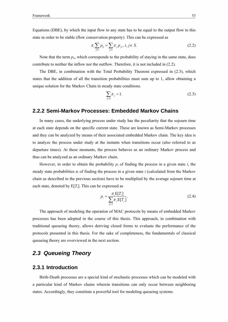
Framework
53
Equations (DBE), by which the input flow to any state has to be equal to the output flow to this
state in order to be stable (flow conservation property). This can be expressed as
, , .i ij j jij i j i
p p i j S
(2.2)
Note that the term pii, which corresponds to the probability of staying in the same state, does
contribute to neither the inflow nor the outflow. Therefore, it is not included in (2.2).
The DBE, in combination with the Total Probability Theorem expressed in (2.3), which
states that the addition of all the transition probabilities must sum up to 1, allow obtaining a
unique solution for the Markov Chain in steady state conditions.
1.jj S
(2.3)
2.2.2 Semi-Markov Processes: Embedded Markov Chains
In many cases, the underlying process under study has the peculiarity that the sojourn time
at each state depends on the specific current state. These are known as Semi-Markov processes
and they can be analyzed by means of their associated embedded Markov chain. The key idea is
to analyze the process under study at the instants when transitions occur (also referred to as
departure times). At these moments, the process behaves as an ordinary Markov process and
thus can be analyzed as an ordinary Markov chain.
However, in order to obtain the probability pi of finding the process in a given state i, the
steady state probabilities πi of finding the process in a given state i (calculated from the Markov
chain as described in the previous section) have to be multiplied by the average sojourn time at
each state, denoted by E[Ti]. This can be expressed as
E[ ]
.E[ ]
i ii
j jj S
Tp
T
(2.4)
The approach of modeling the operation of MAC protocols by means of embedded Markov
processes has been adopted in the course of this thesis. This approach, in combination with
traditional queueing theory, allows deriving closed forms to evaluate the performance of the
protocols presented in this thesis. For the sake of completeness, the fundamentals of classical
queueing theory are overviewed in the next section.
2.3 Queueing Theory
2.3.1 Introduction
Birth-Death processes are a special kind of stochastic processes which can be modeled with
a particular kind of Markov chains wherein transitions can only occur between neighboring
states. Accordingly, they constitute a powerful tool for modeling queueing systems.
Chapter II 54
DeparturesArrivals
Queue Server
Queueing System
Population
Figure 2.1 Queueing System with One Server
An example of generic queueing system is illustrated in Figure 2.1. Imagine, for example, a
toll in a highway as a queueing system. The arrival of a new car (customer) to the toll can be
seen as a birth to the system. The car might wait a certain time in the line of cars until it gets to
the toll booth. Eventually, it gets to the first position of the queue and gets ready to pay. The
payment lasts for a certain time, after which, the car (customer) will leave the toll generating a
departure or a death.
The behavior of this kind of queueing system can be modeled with a birth-death Markov
chain. This modeling allows calculating different performance parameters such as the average
waiting or service times and average number of customers in the system, among many others.
The analysis of queueing systems can be very useful for the dimensioning or performance
analysis of telecommunication systems. There are in the literature several books [1]-[4] and
journals related to the analysis of different types of queueing systems and network of queues,
i.e., networks of interconnected queueing systems. The purpose of this section is to define the
few concepts that will be used for the analysis henceforth.
2.3.2 Kendall’s Notation
Kendall’s notation allows characterizing a queueing system in a very compact manner. Any
queueing server can be basically described with a triplet A/B/m. A denotes the interarrival
distribution, B denotes the service time distribution, and m indicates the number of servers in the
queueing system, i.e., the number of customers that can be served simultaneously. A and B
usually take the following values: M (exponential), D (deterministic) or G (general).
Occasionally, some other values can be also used to define different time distributions. This
nomenclature can be extended to consider storage capacities or finite populations as
comprehensively reported in [1].
2.3.3 Stability Condition
The analysis of queueing systems can only be done in stable conditions, i.e., when the
arrival rate of a system denoted by is at most equal to the mean service rate of the system,
denoted by . Therefore, if is defined as the utilization factor of the system, i.e., the
proportion of time the server is busy, the stability condition can be expressed as
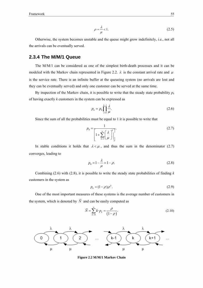
Framework
55
1.
(2.5)
Otherwise, the system becomes unstable and the queue might grow indefinitely, i.e., not all
the arrivals can be eventually served.
2.3.4 The M/M/1 Queue
The M/M/1 can be considered as one of the simplest birth-death processes and it can be
modeled with the Markov chain represented in Figure 2.2. is the constant arrival rate and
is the service rate. There is an infinite buffer at the queueing system (no arrivals are lost and
they can be eventually served) and only one customer can be served at the same time.
By inspection of the Markov chain, it is possible to write that the steady state probability pk
of having exactly k customers in the system can be expressed as
1
00
.k
ki
p p
(2.6)
Since the sum of all the probabilities must be equal to 1 it is possible to write that
0
1
1.
1k
k
p
(2.7)
In stable conditions it holds that , and thus the sum in the denominator (2.7)
converges, leading to
0 1 1 .p
(2.8)
Combining (2.6) with (2.8), it is possible to write the steady state probabilities of finding k
customers in the system as
(1 ) .kkp (2.9)
One of the most important measures of these systems is the average number of customers in
the system, which is denoted by N and can be easily computed as
0
· .1k
k
N k p
(2.10)
Figure 2.2 M/M/1 Markov Chain
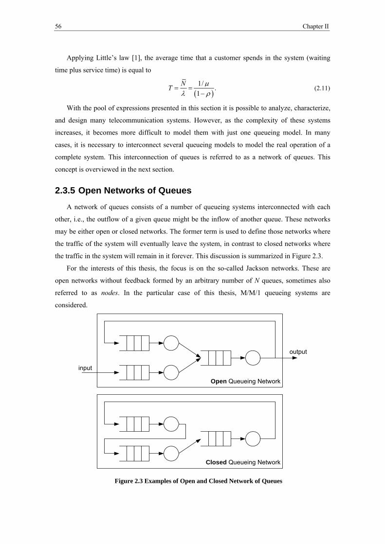
Chapter II 56
Applying Little’s law [1], the average time that a customer spends in the system (waiting
time plus service time) is equal to
1/
.1
NT
(2.11)
With the pool of expressions presented in this section it is possible to analyze, characterize,
and design many telecommunication systems. However, as the complexity of these systems
increases, it becomes more difficult to model them with just one queueing model. In many
cases, it is necessary to interconnect several queueing models to model the real operation of a
complete system. This interconnection of queues is referred to as a network of queues. This
concept is overviewed in the next section.
2.3.5 Open Networks of Queues
A network of queues consists of a number of queueing systems interconnected with each
other, i.e., the outflow of a given queue might be the inflow of another queue. These networks
may be either open or closed networks. The former term is used to define those networks where
the traffic of the system will eventually leave the system, in contrast to closed networks where
the traffic in the system will remain in it forever. This discussion is summarized in Figure 2.3.
For the interests of this thesis, the focus is on the so-called Jackson networks. These are
open networks without feedback formed by an arbitrary number of N queues, sometimes also
referred to as nodes. In the particular case of this thesis, M/M/1 queueing systems are
considered.
Open Queueing Network
Closed Queueing Network
input
output
Figure 2.3 Examples of Open and Closed Network of Queues
Framework
57
The service rate at queue i is i and there is a source which generates Poisson distributed
arrivals to the network with arrival rate . In these networks, it is not possible to ensure that all
the input/output of each of the systems in the network is a Poisson process. However, Jackson’s
theorem states that in stable conditions, i.e., / 1 , each of the 1..N queues forming the
network behave as independent queueing systems and they act as if the input to each of the
queues were Poisson distributed [5]. Consequently, it is possible to write that
1 2 1 1 2 2( , ,... ) ( ) ( )··· ( ).N N Np k k k p k p k p k (2.12)
pi(ki) denotes the equilibrium probability of finding ki users at queue i and p(k1, k2, …kN) is
the joint probability of finding at a given time exactly k1 users at queue 1 and k2 users at queue 2
and so on.
In the specific case of networks of M/M/1 queues and according to the analysis presented in
the previous section, it is possible to write that
11
( ,..., ) (1 ) .i
Nk
N i ii
p k k
(2.13)
where i is the utilization factor of queue i. Finally, the utilization factor of the entire network
can be written as
1 1
1 (0,0,...,0) 1 (0) 1 (1 ).N N
ii i
p p
(2.14)
This last result is very important for the analyses presented in the thesis. It allows
computing in an easy manner the utilization factor of a tandem (or sequence) of queues, which
can be interpreted as the probability that there is at least one user in the system. In other words,
it represents the probability that the system is busy in a given point in time.
2.4 Computer Simulation
2.4.1 Motivation
Due to the limitations of current analytical models for ad hoc networks and the time-costs of
deploying real implementations many researchers decide to study the performance of MAC
protocols by means of computer simulations. In fact, in an ideal world, the development of novel
protocols and schemes would be accompanied by real implementations using either off-the-shelf
products or software defined radios. These implementations would allow evaluating the different
alternatives in order to select the best protocols or algorithms to be deployed in commercial or
real equipment. However, such an approach would be extremely time-consuming and the human-
effort cost would be unacceptable in most cases.
Testbeds constitute an alternative; they emulate a real system by interconnecting different
devices (computers, routers, mobile phones, etc.) which assume different roles and thus emulate
Chapter II 58
the different players involved in a real system. Unfortunately, the costs of the deployment of
testbeds are still considerably high (in terms both of time and money) and their maintenance is in
most cases unaffordable, especially if mobility has to be considered. In addition, there are almost
no open-firmware devices in the market and thus it is sometimes difficult to implement
completely new technologies or communication protocols. For this reason, testbeds usually are
strongly standard-based.
Therefore, computer simulations constitute a useful alternative for overcoming the
difficulties found when deploying either actual prototypes or emulation testbeds. Indeed,
computer simulations are the fastest and most efficient solution. However, if the results obtained
by simulation have to be similar to those that would be obtained in real life, it is necessary to
create as realistic simulation models as possible. As reported in [6], the results presented in
several research works may be questionable due to the simplifications carried out in the
simulations. A different report presented in [7] also shows by comparing simulation results with
real measurements that most of the already existing simulation tools fail in successfully
simulating real networks. The final conclusion of those two works is that the (relatively) small
details omitted in a simulation may have a great impact on the results obtained by simulation and
thus on the conclusions that can be inferred from them. According to that, any simulation tool
should strive to model a network “as real as possible”. However, it is almost impossible to take
into account all the small details of the real world and thus some simplifications have to be done.
The criteria to do so depend on the specific aim of the design; acceptable simplifications for the
simulation of a routing protocol may be completely different to those acceptable to simulate a
coding scheme at the PHY layer. In addition, there is a tradeoff between accuracy and efficiency
of the simulator. The more details considered in the model, the more complex the simulation
becomes, and thus the longer it takes. Therefore, irrelevant details must be omitted.
It must also be mentioned that the mismatch between simulation and real measurements also
stems from the fact that the variability of the radio channel and the amount of interrelated agents
that influence the performance of wireless communications make it very difficult to capture the
exact configuration of a network. In addition, some simplifications are usually assumed in real
measurements so that it is possible to repeat a same experiment many times without depending
on external variable agents.
Therefore, the open question is which the best simulation tool to work with is. In answer to
this, it is also discussed in [7] that the results obtained with different simulators for the same
scenario may vary significantly. This is due to the different criteria used in each simulator to
introduce simplifications. Therefore, it is not clear which is the best simulation tool to be used for
research. As expected, there is no best simulation tool for all cases, but the selection of a tool will
depend on the focus of the research. Although some researchers unconditionally promote the use
Framework
59
of well known simulation tools, there are some issues that might be taken into account and which
are sometimes omitted.
This is the case, for example, of OPNET [8]. OPNET is a relatively expensive commercial
package which works on the basis of time-limited licenses. Funding available today might not be
available tomorrow, and this is a risk that can defer some research groups from choosing it as a
simulation tool. In addition, OPNET is suitable for evaluation of communication systems at the
system-level, but is not as suitable for simulation of the lower layers of the protocol stack.
Another example is the Network Simulator-2 (ns-2) [9], which is arguably the most
extended platform in the networking research field. It is a widely used event-driven simulation
tool that provides substantial support for simulation of MAC protocols over wireless networks.
It is an open-source simulator that runs under Linux. It is also accompanied by the Network
Animator (also known as nam), which is an animation tool for viewing network simulation
traces and real world packet traces with a per-packet granularity. However, it has the following
drawbacks:
1) It is a very difficult tool to master. There is so much source code available that the
knowledge of all the functions and its complete operation implies a long-term learning
process. The perfect knowledge of any simulator is essential in order to be able to
understand the results obtained from any simulation.
2) There are so many people working on ns-2 that there is some degree of inconsistency
among the different versions.
3) It is a good tool to simulate 802.11-based protocols and slight variations of these
protocols, but it might not be suitable to integrate completely new approaches with
innovative mechanisms that affect different layers.
In addition, not only these two but also most of the existing simulators (Glomosim [10] and
OMNet++ [11], among many others) have been developed to cover a wide range of
communication layers, making them flexible and suitable for many researchers all over the
world. Unfortunately, this flexibility also yields suboptimal performance in each of the specific
topics, leading to long simulation periods that may make them not suitable for protocol design,
but for overall system performance evaluation.
In the view of the author, no simulator can mimic the real world with 100% fidelity.
However, this should not be the aim of computer simulation. Assuming that a sufficient degree
of fidelity with the real world is achieved, the real value of computer simulations is the
capability to easily compare the performance of different protocols and, more important, to
evaluate trends in the performance of communication protocols.
Considering these issues, the MACSWIN simulator has been developed within the context of
this thesis as a new simulation tool specifically aimed at the design and performance evaluation
of novel MAC protocols for wireless ad hoc networks. It has the following main features:
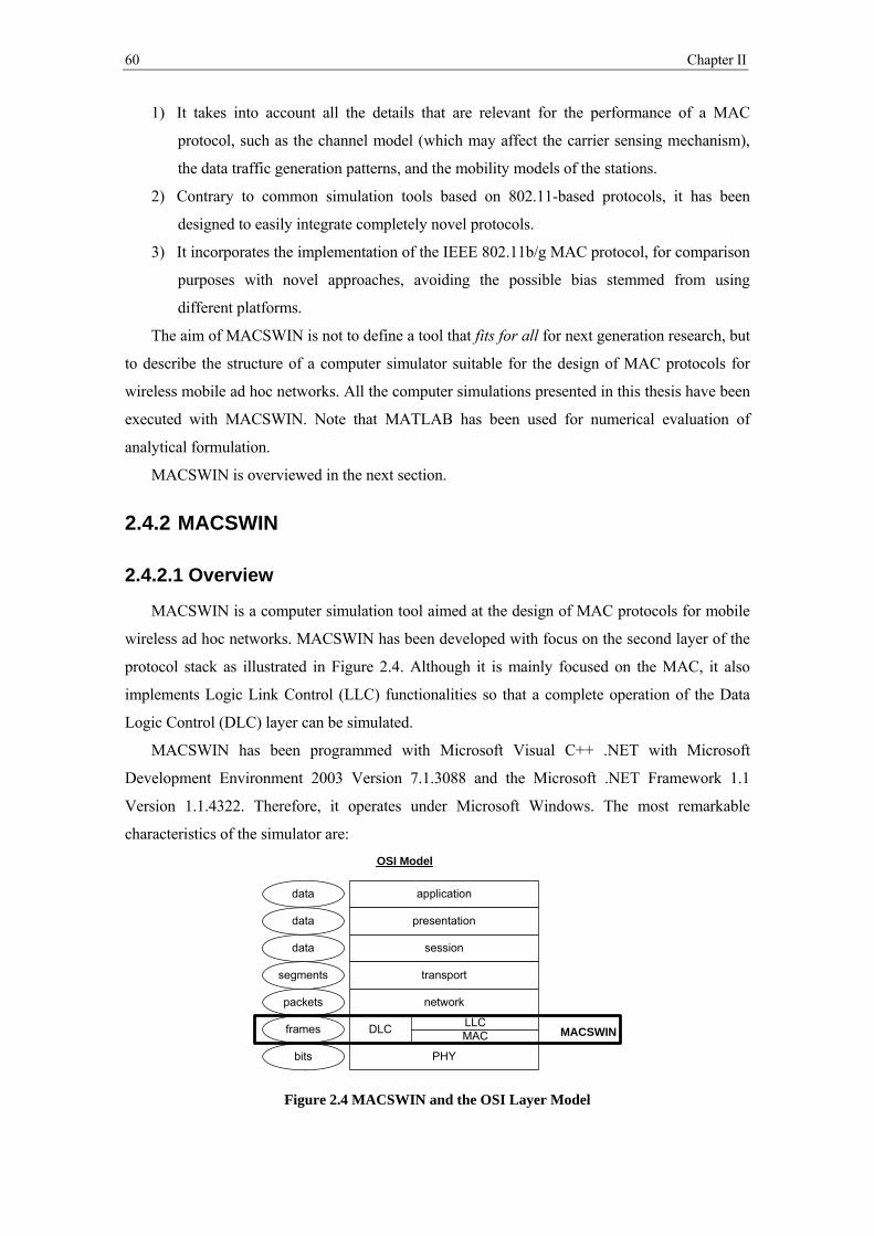
Chapter II 60
1) It takes into account all the details that are relevant for the performance of a MAC
protocol, such as the channel model (which may affect the carrier sensing mechanism),
the data traffic generation patterns, and the mobility models of the stations.
2) Contrary to common simulation tools based on 802.11-based protocols, it has been
designed to easily integrate completely novel protocols.
3) It incorporates the implementation of the IEEE 802.11b/g MAC protocol, for comparison
purposes with novel approaches, avoiding the possible bias stemmed from using
different platforms.
The aim of MACSWIN is not to define a tool that fits for all for next generation research, but
to describe the structure of a computer simulator suitable for the design of MAC protocols for
wireless mobile ad hoc networks. All the computer simulations presented in this thesis have been
executed with MACSWIN. Note that MATLAB has been used for numerical evaluation of
analytical formulation.
MACSWIN is overviewed in the next section.
2.4.2 MACSWIN
2.4.2.1 Overview
MACSWIN is a computer simulation tool aimed at the design of MAC protocols for mobile
wireless ad hoc networks. MACSWIN has been developed with focus on the second layer of the
protocol stack as illustrated in Figure 2.4. Although it is mainly focused on the MAC, it also
implements Logic Link Control (LLC) functionalities so that a complete operation of the Data
Logic Control (DLC) layer can be simulated.
MACSWIN has been programmed with Microsoft Visual C++ .NET with Microsoft
Development Environment 2003 Version 7.1.3088 and the Microsoft .NET Framework 1.1
Version 1.1.4322. Therefore, it operates under Microsoft Windows. The most remarkable
characteristics of the simulator are:
application
presentation
session
transport
network
DLC
PHY
LLCMAC
data
data
data
segments
packets
frames
bits
MACSWIN
OSI Model
Figure 2.4 MACSWIN and the OSI Layer Model
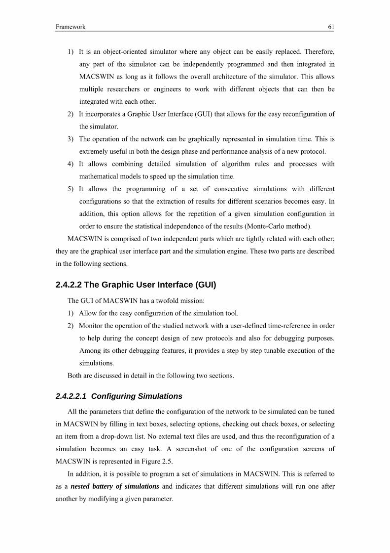
Framework
61
1) It is an object-oriented simulator where any object can be easily replaced. Therefore,
any part of the simulator can be independently programmed and then integrated in
MACSWIN as long as it follows the overall architecture of the simulator. This allows
multiple researchers or engineers to work with different objects that can then be
integrated with each other.
2) It incorporates a Graphic User Interface (GUI) that allows for the easy reconfiguration of
the simulator.
3) The operation of the network can be graphically represented in simulation time. This is
extremely useful in both the design phase and performance analysis of a new protocol.
4) It allows combining detailed simulation of algorithm rules and processes with
mathematical models to speed up the simulation time.
5) It allows the programming of a set of consecutive simulations with different
configurations so that the extraction of results for different scenarios becomes easy. In
addition, this option allows for the repetition of a given simulation configuration in
order to ensure the statistical independence of the results (Monte-Carlo method).
MACSWIN is comprised of two independent parts which are tightly related with each other;
they are the graphical user interface part and the simulation engine. These two parts are described
in the following sections.
2.4.2.2 The Graphic User Interface (GUI)
The GUI of MACSWIN has a twofold mission:
1) Allow for the easy configuration of the simulation tool.
2) Monitor the operation of the studied network with a user-defined time-reference in order
to help during the concept design of new protocols and also for debugging purposes.
Among its other debugging features, it provides a step by step tunable execution of the
simulations.
Both are discussed in detail in the following two sections.
2.4.2.2.1 Configuring Simulations
All the parameters that define the configuration of the network to be simulated can be tuned
in MACSWIN by filling in text boxes, selecting options, checking out check boxes, or selecting
an item from a drop-down list. No external text files are used, and thus the reconfiguration of a
simulation becomes an easy task. A screenshot of one of the configuration screens of
MACSWIN is represented in Figure 2.5.
In addition, it is possible to program a set of simulations in MACSWIN. This is referred to
as a nested battery of simulations and indicates that different simulations will run one after
another by modifying a given parameter.
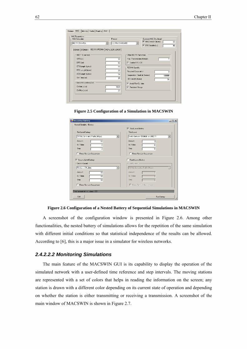
Chapter II 62
Figure 2.5 Configuration of a Simulation in MACSWIN
Figure 2.6 Configuration of a Nested Battery of Sequential Simulations in MACSWIN
A screenshot of the configuration window is presented in Figure 2.6. Among other
functionalities, the nested battery of simulations allows for the repetition of the same simulation
with different initial conditions so that statistical independence of the results can be allowed.
According to [6], this is a major issue in a simulator for wireless networks.
2.4.2.2.2 Monitoring Simulations
The main feature of the MACSWIN GUI is its capability to display the operation of the
simulated network with a user-defined time reference and step intervals. The moving stations
are represented with a set of colors that helps in reading the information on the screen; any
station is drawn with a different color depending on its current state of operation and depending
on whether the station is either transmitting or receiving a transmission. A screenshot of the
main window of MACSWIN is shown in Figure 2.7.
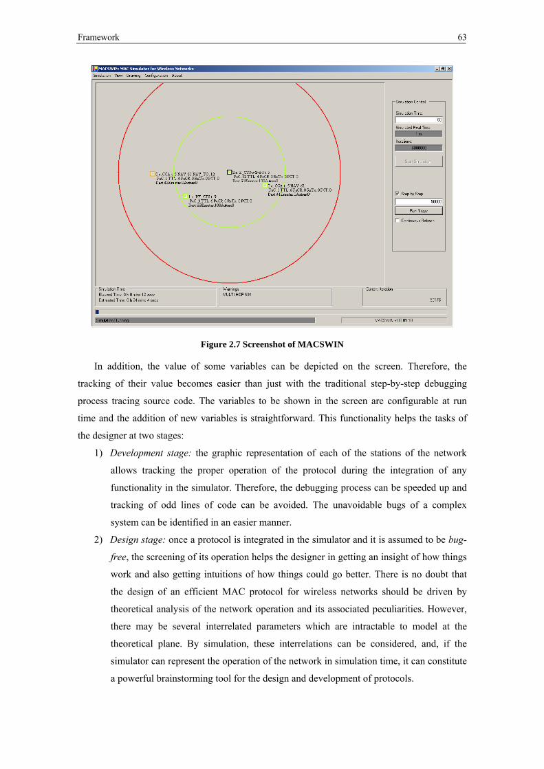
Framework
63
Figure 2.7 Screenshot of MACSWIN
In addition, the value of some variables can be depicted on the screen. Therefore, the
tracking of their value becomes easier than just with the traditional step-by-step debugging
process tracing source code. The variables to be shown in the screen are configurable at run
time and the addition of new variables is straightforward. This functionality helps the tasks of
the designer at two stages:
1) Development stage: the graphic representation of each of the stations of the network
allows tracking the proper operation of the protocol during the integration of any
functionality in the simulator. Therefore, the debugging process can be speeded up and
tracking of odd lines of code can be avoided. The unavoidable bugs of a complex
system can be identified in an easier manner.
2) Design stage: once a protocol is integrated in the simulator and it is assumed to be bug-
free, the screening of its operation helps the designer in getting an insight of how things
work and also getting intuitions of how things could go better. There is no doubt that
the design of an efficient MAC protocol for wireless networks should be driven by
theoretical analysis of the network operation and its associated peculiarities. However,
there may be several interrelated parameters which are intractable to model at the
theoretical plane. By simulation, these interrelations can be considered, and, if the
simulator can represent the operation of the network in simulation time, it can constitute
a powerful brainstorming tool for the design and development of protocols.
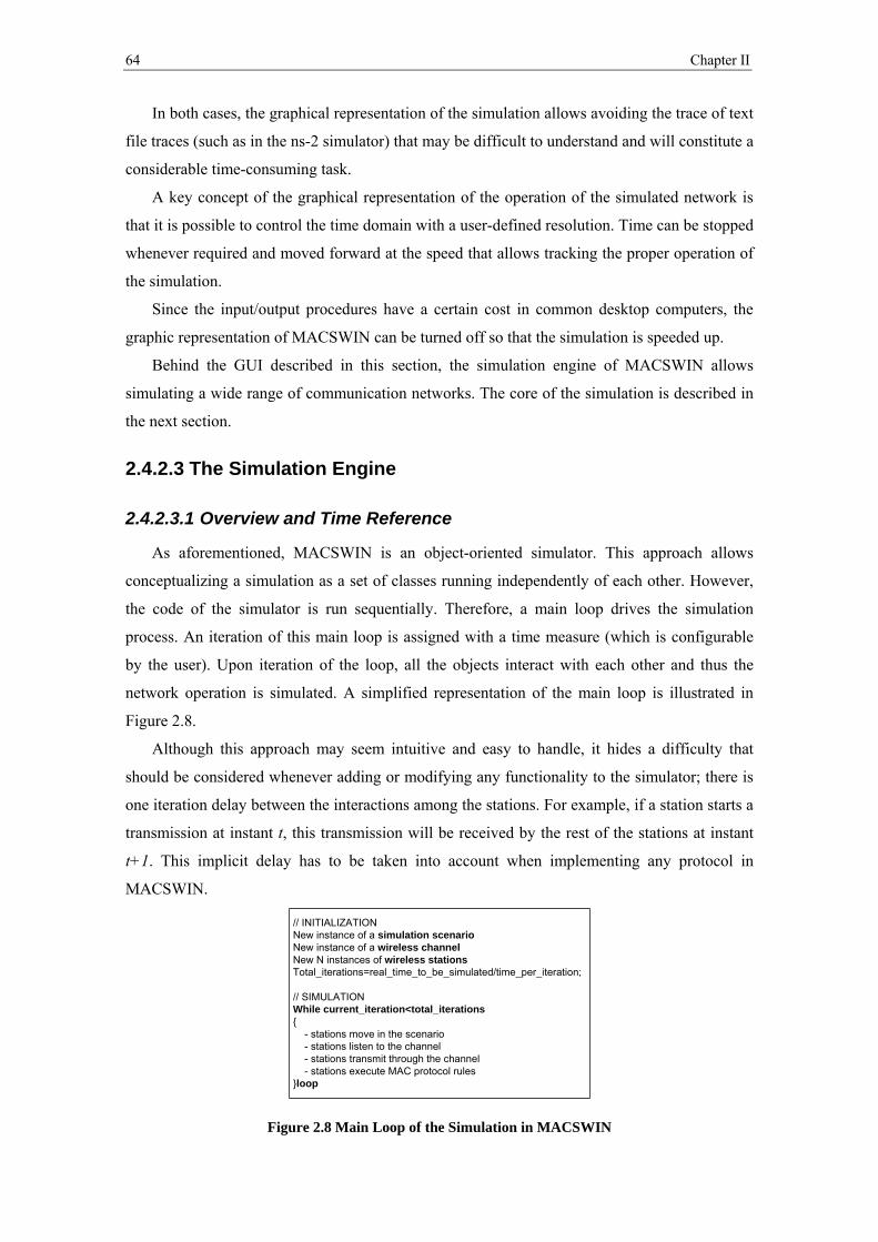
Chapter II 64
In both cases, the graphical representation of the simulation allows avoiding the trace of text
file traces (such as in the ns-2 simulator) that may be difficult to understand and will constitute a
considerable time-consuming task.
A key concept of the graphical representation of the operation of the simulated network is
that it is possible to control the time domain with a user-defined resolution. Time can be stopped
whenever required and moved forward at the speed that allows tracking the proper operation of
the simulation.
Since the input/output procedures have a certain cost in common desktop computers, the
graphic representation of MACSWIN can be turned off so that the simulation is speeded up.
Behind the GUI described in this section, the simulation engine of MACSWIN allows
simulating a wide range of communication networks. The core of the simulation is described in
the next section.
2.4.2.3 The Simulation Engine
2.4.2.3.1 Overview and Time Reference
As aforementioned, MACSWIN is an object-oriented simulator. This approach allows
conceptualizing a simulation as a set of classes running independently of each other. However,
the code of the simulator is run sequentially. Therefore, a main loop drives the simulation
process. An iteration of this main loop is assigned with a time measure (which is configurable
by the user). Upon iteration of the loop, all the objects interact with each other and thus the
network operation is simulated. A simplified representation of the main loop is illustrated in
Figure 2.8.
Although this approach may seem intuitive and easy to handle, it hides a difficulty that
should be considered whenever adding or modifying any functionality to the simulator; there is
one iteration delay between the interactions among the stations. For example, if a station starts a
transmission at instant t, this transmission will be received by the rest of the stations at instant
t+1. This implicit delay has to be taken into account when implementing any protocol in
MACSWIN.
// INITIALIZATIONNew instance of a simulation scenarioNew instance of a wireless channelNew N instances of wireless stationsTotal_iterations=real_time_to_be_simulated/time_per_iteration;
// SIMULATIONWhile current_iteration<total_iterations{ - stations move in the scenario - stations listen to the channel - stations transmit through the channel - stations execute MAC protocol rules}loop
Figure 2.8 Main Loop of the Simulation in MACSWIN
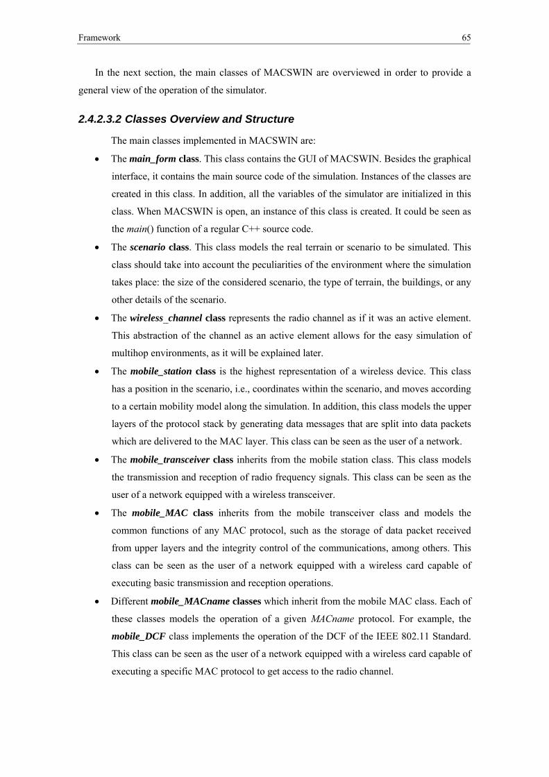
Framework
65
In the next section, the main classes of MACSWIN are overviewed in order to provide a
general view of the operation of the simulator.
2.4.2.3.2 Classes Overview and Structure
The main classes implemented in MACSWIN are:
The main_form class. This class contains the GUI of MACSWIN. Besides the graphical
interface, it contains the main source code of the simulation. Instances of the classes are
created in this class. In addition, all the variables of the simulator are initialized in this
class. When MACSWIN is open, an instance of this class is created. It could be seen as
the main() function of a regular C++ source code.
The scenario class. This class models the real terrain or scenario to be simulated. This
class should take into account the peculiarities of the environment where the simulation
takes place: the size of the considered scenario, the type of terrain, the buildings, or any
other details of the scenario.
The wireless_channel class represents the radio channel as if it was an active element.
This abstraction of the channel as an active element allows for the easy simulation of
multihop environments, as it will be explained later.
The mobile_station class is the highest representation of a wireless device. This class
has a position in the scenario, i.e., coordinates within the scenario, and moves according
to a certain mobility model along the simulation. In addition, this class models the upper
layers of the protocol stack by generating data messages that are split into data packets
which are delivered to the MAC layer. This class can be seen as the user of a network.
The mobile_transceiver class inherits from the mobile station class. This class models
the transmission and reception of radio frequency signals. This class can be seen as the
user of a network equipped with a wireless transceiver.
The mobile_MAC class inherits from the mobile transceiver class and models the
common functions of any MAC protocol, such as the storage of data packet received
from upper layers and the integrity control of the communications, among others. This
class can be seen as the user of a network equipped with a wireless card capable of
executing basic transmission and reception operations.
Different mobile_MACname classes which inherit from the mobile MAC class. Each of
these classes models the operation of a given MACname protocol. For example, the
mobile_DCF class implements the operation of the DCF of the IEEE 802.11 Standard.
This class can be seen as the user of a network equipped with a wireless card capable of
executing a specific MAC protocol to get access to the radio channel.
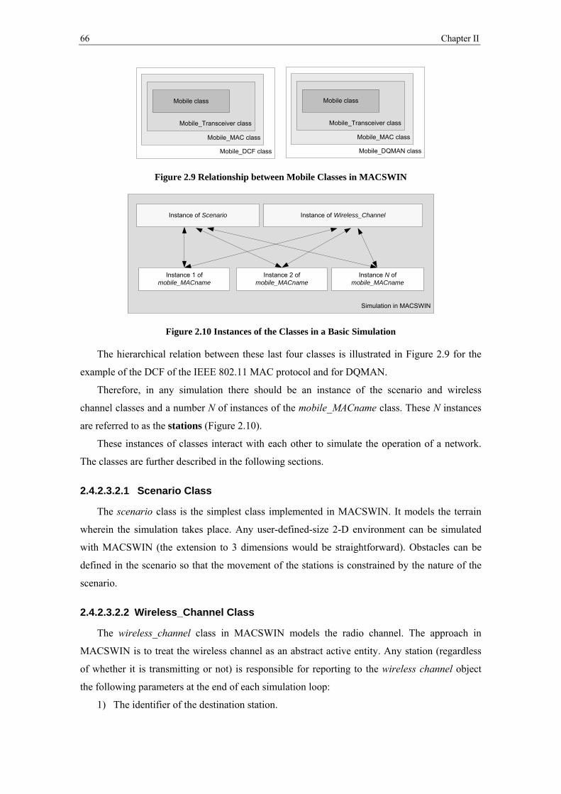
Chapter II 66
Mobile_DCF class
Mobile_MAC class
Mobile_Transceiver class
Mobile class
Mobile_DQMAN class
Mobile_MAC class
Mobile_Transceiver class
Mobile class
Figure 2.9 Relationship between Mobile Classes in MACSWIN
Simulation in MACSWIN
Instance 1 of mobile_MACname
Instance of Scenario Instance of Wireless_Channel
Instance 2 of mobile_MACname
Instance N of mobile_MACname
Figure 2.10 Instances of the Classes in a Basic Simulation
The hierarchical relation between these last four classes is illustrated in Figure 2.9 for the
example of the DCF of the IEEE 802.11 MAC protocol and for DQMAN.
Therefore, in any simulation there should be an instance of the scenario and wireless
channel classes and a number N of instances of the mobile_MACname class. These N instances
are referred to as the stations (Figure 2.10).
These instances of classes interact with each other to simulate the operation of a network.
The classes are further described in the following sections.
2.4.2.3.2.1 Scenario Class
The scenario class is the simplest class implemented in MACSWIN. It models the terrain
wherein the simulation takes place. Any user-defined-size 2-D environment can be simulated
with MACSWIN (the extension to 3 dimensions would be straightforward). Obstacles can be
defined in the scenario so that the movement of the stations is constrained by the nature of the
scenario.
2.4.2.3.2.2 Wireless_Channel Class
The wireless_channel class in MACSWIN models the radio channel. The approach in
MACSWIN is to treat the wireless channel as an abstract active entity. Any station (regardless
of whether it is transmitting or not) is responsible for reporting to the wireless channel object
the following parameters at the end of each simulation loop:
1) The identifier of the destination station.
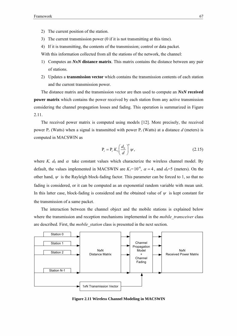
Framework
67
2) The current position of the station.
3) The current transmission power (0 if it is not transmitting at this time).
4) If it is transmitting, the contents of the transmission; control or data packet.
With this information collected from all the stations of the network, the channel:
1) Computes an NxN distance matrix. This matrix contains the distance between any pair
of stations.
2) Updates a transmission vector which contains the transmission contents of each station
and the current transmission power.
The distance matrix and the transmission vector are then used to compute an NxN received
power matrix which contains the power received by each station from any active transmission
considering the channel propagation losses and fading. This operation is summarized in Figure
2.11.
The received power matrix is computed using models [12]. More precisely, the received
power Pr (Watts) when a signal is transmitted with power Pt (Watts) at a distance d (meters) is
computed in MACSWIN as
01P P ,r t
dK
d
(2.15)
where K, d0 and take constant values which characterize the wireless channel model. By
default, the values implemented in MACSWIN are K1=10-6, 4 , and d0=5 (meters). On the
other hand, is the Rayleigh block-fading factor. This parameter can be forced to 1, so that no
fading is considered, or it can be computed as an exponential random variable with mean unit.
In this latter case, block-fading is considered and the obtained value of is kept constant for
the transmission of a same packet.
The interaction between the channel object and the mobile stations is explained below
where the transmission and reception mechanisms implemented in the mobile_transceiver class
are described. First, the mobile_station class is presented in the next section.
Station 0
Station 1
Station 2
Station N-1
NxNDistance Matrix
Channel Propagation
Model +
Channel Fading
NxNReceived Power Matrix
1xN Transmission Vector
Figure 2.11 Wireless Channel Modeling in MACSWIN
Chapter II 68
2.4.2.3.2.3 Mobile_Station Class
As aforementioned, this is the highest representation of a wireless device. This class can be
seen as the user of a network. Three are the main functionalities modeled with this class:
1) Mobility of the stations.
2) Data packet generation at the application layer that are delivered to the MAC layer in
the form of control or data packets.
3) Buffering of data packets until they can be transmitted over the channel.
2.4.2.3.2.3.1 Mobility Model
Every station in the simulation has a current position in the form of Cartesian coordinates
(x,y) and a current speed, expressed in modulus and direction. The position is changed following
one of the mobility models described in [13]. All of them have been integrated in MASCWIN.
These mobility models can be split into two groups, according to whether each station moves
independently of the others, or whether there is some correlation between the movements of
some groups of stations:
1) Individual mobility models: Random walk mobility model, random waypoint mobility
model, random direction mobility model, boundless simulation area mobility model,
Gauss-Markov mobility model, and city section mobility model.
2) Group mobility models: Column mobility model, nomadic mobility model, pursue
mobility model, and reference point mobility model.
The set of mobility models integrated in MACSWIN allows for the realistic simulation of a
wide range of scenarios and network applications.
2.4.2.3.2.3.2 Data Traffic Generation and Buffering
This class implements the generation of data traffic which simulates the arrival of data
packets to the MAC layer from upper layers of the protocol stack.
Three arrival data traffic generation patterns are implemented in MACSWIN:
1) Poisson (exponential) distributed data process with tunable arrival rate expressed in
messages/second.
2) Bernoulli process. A message is generated with probability pg every Tg seconds. These
parameters are automatically adjusted in MACSWIN once the total offered load to the
network is determined in bps. This traffic pattern allows evaluating a network at a given
total offered load.
3) Saturation process that ensures that a station has always at least one message ready to
transmit.
Whenever an arrival is simulated, the length of the message can be:
1) Exponentially distributed length with average M bits.
Framework
69
2) Fixed-length messages.
Whenever a station generates a message, it fragments it into constant-length data packets of
length L bytes. Since the stations do not have immediate access to the radio channel whenever
they have data packets ready to be transmitted, these data packets are stored in buffers.
In MACSWIN, each station is modeled with three First-In First-Out (FIFO) buffers where
data packets can be stored. The three queues allow for buffering user’s data, routing packets,
and forwarding packets (for cooperative simulation).
2.4.2.3.2.4 Mobile_Transceiver Class
In C++ terms, this class inherits from the mobile_station class. This class models the
transmission and reception of radio signals. This class can be seen as the user of a network
equipped with a wireless transceiver.
The functionalities modeled in this class are:
1) The transmission and reception of radio signals (interaction with the channel object).
2) The detection of collisions (interpretation of the channel feedback).
3) The decoding of packets with a certain packet error probability.
4) The power consumption.
The implementation of these functionalities is described in the following sections.
2.4.2.3.2.4.1 Transmission and Reception Model
Whenever a station listens to the channel, it inquires from the channel object to feed back
whether the channel seen by the station is idle or busy. Two signal strength thresholds determine
whether the channel is idle or busy:
1) The Carrier Sensing Threshold (CST) defined as the minimum received signal strength
necessary to determine that the channel is busy.
2) Reception Threshold (RXT) defined as the minimum received signal strength necessary
to attempt to decode an incoming signal.
In the case that the received power of any received signal is over the RXT and no collision
is detected, then the channel provides the station with the received data or control packet. The
collision models included in MACSWIN are described in the next section.
2.4.2.3.2.4.2 Collision Model
One of the major issues when modeling a wireless network is the rule for deciding when a
collision occurs if two or more simultaneous signals are received at any station. Two models are
considered in MACSWIN:
1) Collision model, wherein the reception of two signals over the CST is treated as a
collision.
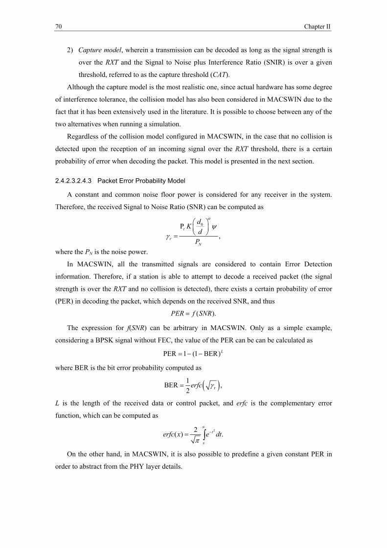
Chapter II 70
2) Capture model, wherein a transmission can be decoded as long as the signal strength is
over the RXT and the Signal to Noise plus Interference Ratio (SNIR) is over a given
threshold, referred to as the capture threshold (CAT).
Although the capture model is the most realistic one, since actual hardware has some degree
of interference tolerance, the collision model has also been considered in MACSWIN due to the
fact that it has been extensively used in the literature. It is possible to choose between any of the
two alternatives when running a simulation.
Regardless of the collision model configured in MACSWIN, in the case that no collision is
detected upon the reception of an incoming signal over the RXT threshold, there is a certain
probability of error when decoding the packet. This model is presented in the next section.
2.4.2.3.2.4.3 Packet Error Probability Model
A constant and common noise floor power is considered for any receiver in the system.
Therefore, the received Signal to Noise Ratio (SNR) can be computed as
0P,
t
rN
dK
dP
where the PN is the noise power.
In MACSWIN, all the transmitted signals are considered to contain Error Detection
information. Therefore, if a station is able to attempt to decode a received packet (the signal
strength is over the RXT and no collision is detected), there exists a certain probability of error
(PER) in decoding the packet, which depends on the received SNR, and thus
( ).PER f SNR
The expression for f(SNR) can be arbitrary in MACSWIN. Only as a simple example,
considering a BPSK signal without FEC, the value of the PER can be can be calculated as
PER 1 (1 BER)L
where BER is the bit error probability computed as
r
1BER ,
2erfc
L is the length of the received data or control packet, and erfc is the complementary error
function, which can be computed as
22
( ) .t
x
erfc x e dt
On the other hand, in MACSWIN, it is also possible to predefine a given constant PER in
order to abstract from the PHY layer details.
Framework
71
2.4.2.3.2.4.4 Power Consumption
The simulator tracks the power consumption associated to each station, both instantaneously
and averaged along the simulation time. The measurements are normalized to the power
consumption associated with the transmit energy consumption and they distinguish between:
1) TRANSMIT consumption, representing the energy consumption of a transmitting station.
2) RECEPTION consumption, representing the energy consumption of a station sensing
the channel busy and attempting to decode an incoming signal.
3) IDLE consumption, representing the energy consumed by a station sensing the channel
idle.
4) SLEEP consumption, representing the energy consumption of a switched-off station.
2.4.2.3.2.5 Mobile_MAC and Mobile_MACname Class
The mobile_MAC class models the most common functions of the MAC protocol, such as
the channel sensing, the ARQ algorithm, and the fetching of data packets from the buffers,
among others.
However, the rules of the MAC protocol are implemented in a specific class that inherits all
the functionalities of the mobile_MAC class, namely the mobile_MACname class. The specific
name of this class depends on the implemented MAC protocol. This class, independently of the
MAC protocol it implements, inherits all the functionalities of the mobile_transceiver class,
which in turn inherits all the functionalities of the mobile_station class. This inheritance
relationship between mobile classes in MACSWIN was depicted in Figure 2.9.
In any simulation, there will be an instance of a mobile_MACname class for each station.
The MAC protocols implemented in MACSWIN, and their respective classes, are:
1) DCF of the IEEE 802.11 Standard mobile_DCF.
2) PCF of the IEEE 802.11 Standard mobile_PCF.
3) DQMAN protocol, presented in Chapter III mobile_DQMAN.
4) DPCF protocol, presented in Chapter IV mobile_DPCF.
5) DQCOOP protocol, presented in Chapter V mobile_DQCOOP.
6) PRCSMA protocol, presented in Chapter V mobile_PRCSMA.
Any MAC protocol in MACSWIN is conceptualized as a multiple state-machine. A station
has a current state and switches to any other state in a loop iteration according to the
interactions with the channel object and with other stations. For example, a simplified state-
machine of a basic IEEE 802.11 station implemented in MACSWIN is illustrated in Figure
2.12, where the circles represent the different states implemented in the mobile_DCF class. An
overview of the DCF is presented in Section 4.3.1 of Chapter IV.
An IEEE 802.11 station remains in the idle state as long as the channel is sensed idle and it
has no data packet to transmit. Whenever it has a data packet ready to be transmitted, it switches
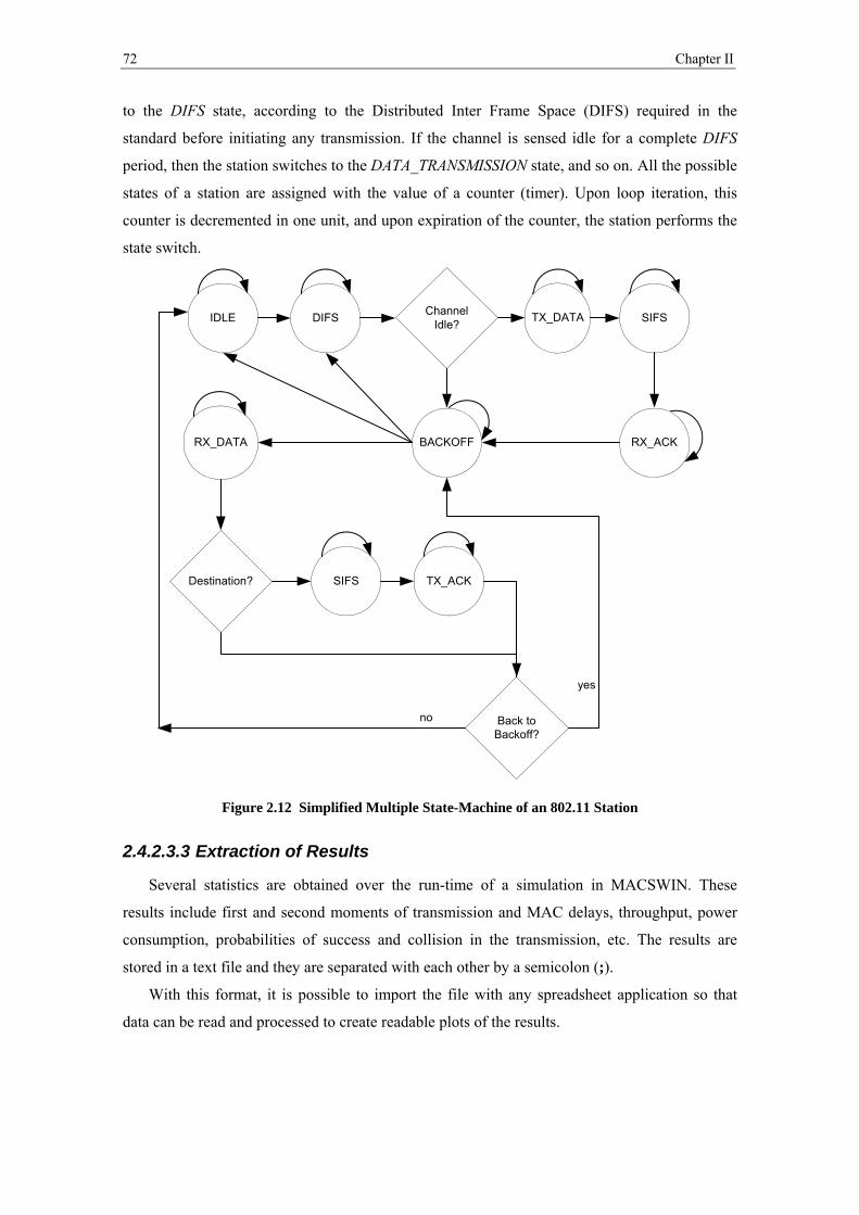
Chapter II 72
to the DIFS state, according to the Distributed Inter Frame Space (DIFS) required in the
standard before initiating any transmission. If the channel is sensed idle for a complete DIFS
period, then the station switches to the DATA_TRANSMISSION state, and so on. All the possible
states of a station are assigned with the value of a counter (timer). Upon loop iteration, this
counter is decremented in one unit, and upon expiration of the counter, the station performs the
state switch.
IDLE DIFS TX_DATA
RX_DATA BACKOFF
Channel Idle?
Back toBackoff?
SIFS
Destination? SIFS
RX_ACK
TX_ACK
yes
no
Figure 2.12 Simplified Multiple State-Machine of an 802.11 Station
2.4.2.3.3 Extraction of Results
Several statistics are obtained over the run-time of a simulation in MACSWIN. These
results include first and second moments of transmission and MAC delays, throughput, power
consumption, probabilities of success and collision in the transmission, etc. The results are
stored in a text file and they are separated with each other by a semicolon (;).
With this format, it is possible to import the file with any spreadsheet application so that
data can be read and processed to create readable plots of the results.
Framework
73
2.5 References
[1] L. Kleinrock, “Queueing Systems, Volume I: Theory,” Wiley Interscience, 1975.
[2] R. W. Wolff, “Stochastic Modeling and the Theory of Queues,” Prentice Hall, 1989.
[3] A. Kumar, D. Manjunath, and J.Kuri, “Communication Networking, an analytical
approach,” Morgan Kauffman, 2004.
[4] R. Nelson, “Probability, Stochastic Processes and Queueing Theory,” Springer-Verlag,
1995.
[5] J. R. Jackson, “Networks of waiting lines,” Operations Research, vol.5, no. 4, 518-521,
1957.
[6] T. R. Andel and A. Yasinac, “On the Credibility of MANET Simulations,” IEEE
Computer, Jun. 2006.
[7] B. Schilling and J. Hahner, “Qualitative Comparison of Network Simulator Tools,”
Institute of Parallel and Distributed Systems, Jan. 2005.
[8] OPNET modeler, http://www.opnet.com/
[9] The Network Simulator (NS-2), http://isi.edo/nsnam/ns
[10] The Global Mobile Information Systems Simulation Library:
http://pcl.cs.ucla.edu/projects/glomosim.
[11] OMNet, Discrete Event Simulation System, http://www.omnetpp.org.
[12] A. J. Goldsmith, Wireless Communications, Cambridge University Press, 2005.
[13] T. Camp, J. Boleng, and V. Davies, “A Survey of Mobility Models for Ad Hoc Network
Research,” Department of Mathematics and Computer Sciences, Colorado School,
2002.

75
Chapter III
3 A Novel MAC Protocol: DQMAN
3.1 Introduction
The Distributed Queueing MAC protocol for Ad hoc Networks (DQMAN) is presented in
this chapter as an innovative step forward towards the optimal operation for ad hoc networks,
such as WLANs without infrastructure.
DQMAN combines a distributed dynamic clustering algorithm based on carrier sensing
(CSMA) [1] with a near-optimum infrastructure-based MAC protocol, namely the Distributed
Queueing with Collision Avoidance (DQCA) protocol [2]. By integrating a spontaneous,
temporary, and dynamic clustering mechanism into the MAC layer, DQMAN extends the
stability and the high-efficiency of DQCA to a completely distributed network without
infrastructure. The concept and motivation are represented in Figure 3.1
DQMAN can run on top of any PHY layer and thus the ideas presented here are applicable
to any network architecture which can operate in an ad hoc fashion, such as IEEE 802.11b/g,
Chapter III
76
WiMAX (IEEE 802.16), Bluetooth, IRA (Infra-Red Access), or Zigbee (IEEE 802.15.4), among
others.
To the best of our knowledge, the approach of integrating a CSMA-based dynamic and
spontaneous clustering mechanism into the MAC layer has never been tackled before in the
literature. Typically clustering has been applied either at higher layers of the protocol stack
(e.g., for routing) or at the MAC layer only within the context of multi-channel protocols,
wherein each cluster works in a different frequency. In addition, it has been traditionally
accepted the idea that the more stable the cluster structure, the better. In DQMAN, a new
clustering paradigm is presented.
The key idea behind DQMAN is that whenever a station seizes the channel to transmit its
data packets by executing a distributed access mechanism similar to that of the Distributed
Coordination Function (DCF) of the IEEE 802.11 Standard [3], it establishes a temporary one-
hop cluster structure. Recall that the DCF of the IEEE 802.11 Standard is based on CSMA with
Collision Avoidance, which is suitable for operation in infrastructureless networks. The station
which successfully seizes the channel becomes a temporary clusterhead and it coordinates the
data transmissions of all the stations within its transmission range for a bounded period of time.
The protocol running within each cluster is a variation of the near-optimum DQCA protocol for
infrastructure-based WLANs presented in [2]. In its turn, DQCA is based on the Distributed
Queueing Random Access Protocol (DQRAP) presented by Xu and Campbell in [4], initially
designed for the distribution of Cable TV. DQRAP exhibits a near-optimum performance
independently of the amount of active terminals and the offered data traffic. It achieves the
throughput performance of an ideal M/M/1 system and is stable for any input rate even
temporarily beyond the channel capacity. Since then, and due to the outstandingly near-
optimum performance of DQRAP, some efforts have been done to adapt this two-distributed
queue concept to different environments. This is the case of the Extended DQRAP (XDQRAP)
[5], the Prioritized DQRAP (PDQRAP) [6] for wired centralized networks, the Interleaved
DQRAP for satellite applications with long propagation delays [7], and the DQRAP for Code
Division Multiple Access (DQRAP/CDMA), conceived for 3G cellular networks [8].
Distributed Operation
High EfficiencyHierarchical Clustering
Centralized Medium Access Control
DQMAN
DQCACSMA based
Figure 3.1 Concept Design of DQMAN
A Novel MAC Protocol: DQMAN
77
DQMAN constitutes an innovative concept design within the context of MAC protocols for
wireless ad hoc networks. It allows extending the ideas of DQCA to infrastructureless networks,
although the approach could be easily generalized to extend any other centralized MAC
protocol to an infrastructureless network. Indeed, an example of this is presented in Chapter IV
of this thesis, where the Point Coordination Function (PCF) of the IEEE 802.11 Standard is
extended to operate over distributed networks without infrastructure.
3.2 Chapter Structure
The DQMAN protocol is comprehensively described and analyzed throughout the
following sections of this chapter. In Section 3.3 some previous considerations and definitions
are presented. The clustering algorithm of DQMAN is presented in Section 3.4, while Section
3.5 is devoted to the description of the MAC protocol executed within each temporary cluster.
Some operational and implementation issues are then discussed in Section 3.7. The performance
of the protocol in single-hop networks is comprehensively analyzed in Section 3.8. First, the
saturation throughput of DQMAN is analyzed by modeling the clustering algorithm with an
embedded Markov chain. Then, the model is extended to arbitrary traffic loads in order to
compute the throughput, average transmission delay, and some clustering metrics of a network
running DQMAN at the MAC layer.
In Section 3.9 two modifications of the basic operation of the protocol are proposed to
enhance its efficiency in single-hop networks and under heavy traffic conditions. Then, the
performance of DQMAN in multi-hop environments is assessed in Section 3.10.
Section 3.11 describes a methodology that makes possible the coexistence and
intercommunication of DQMAN devices with IEEE 802.11 Standard wireless cards. This study
is necessary in the light of the commercial development of the protocol, since it is hardly
realistic to believe that any new protocol will replace existing standards no matter how much
better performance it may attain. Backwards compatibility is a desirable characteristic for the
success of any new technology.
Finally, Section 3.12 concludes the chapter by summarizing the key contents of the chapter
and highlighting the most relevant results.
3.3 Previous Considerations
DQMAN is designed within the context of distributed networks without infrastructure. It is
assumed that the protocol rules are executed independently and asynchronously at each station,
i.e., in a fully distributed manner.
All the transmissions, even the control packets, are performed in a single-channel. This
corresponds to an in-band signaling scheme. Stations are equipped with a single half-duplex
Chapter III
78
radio transceiver. Therefore, a station can transmit and receive radio signals, but it cannot
perform both functions at the same time. The turn-around time to switch from transmission to
reception mode is non-negligible and is taken into account in the design of the protocol.
In this chapter, a discrete and integer slotted time scale where t and t+1 correspond to the
beginning of two consecutive time units (slots) is considered for the operation of DQMAN.
Therefore, the time unit is the time slot. As in the IEEE 802.11 Standard [3], this parameter is
defined at the PHY layer and is usually referred to as the SlotTime and denoted by . For
example, the default value of this slot time in the 802.11b and g Standards is either 10 µs or 16
µs, and its duration is independent of the MAC rules. Without loss of generality and unless
otherwise stated, 10 µs will be the default value considered in this thesis.
Mimicking the IEEE 802.11 Standard, it is considered that MAC Service Data Units
(MSDU) or MAC Management Data Units (MMDU) delivered to the MAC from higher layers,
are fragmented into smaller MAC Protocol Data Units (MPDU). This is known as the
fragmentation of a message into data packets or fragments. Once a station seizes the channel,
it is usually allowed to transmit all the fragments of a complete message, although this is not a
necessary condition. For example, in the DCF of the 802.11 Standard, all the fragments of a
message can be transmitted with a single access invocation (unless interrupted due to medium
occupancy limitations for a given PHY), while in the PCF of the 802.11 Standard each packet is
transmitted as an individual entity. In this chapter it is considered that all the fragments of the
same message can be transmitted with only one channel access invocation.
In addition, and for the sake of simplicity, each fragment must be acknowledged by the
destination so that the next fragment can be transmitted, i.e., Stop&Wait ARQ is considered. A
PHY preamble and a MAC header are attached to each data packet in order to allow for PHY
synchronization and channel estimation as well as for other MAC functions, such as addressing
and error detection/correction. This is illustrated in Figure 3.2.
Although transmission rates can be dynamically adjusted when available, it will be assumed
that control information is always transmitted at the lowest available transmission rate so as to
maximize its reliability, as in the IEEE 802.11 Standard.
MSDU or MMDU (message)
MPDU MPDU MPDU MPDU
A message from upper layers is fragmented at the
MAC layer into smaller data packets or fragments
Data PayloadMAC headerPHY preamble
A PHY preamble and a MAC header is attached to each MPDU when delivered to the PHY layer
An ACK is expected for each MPDU before processing the
next MPDU
Figure 3.2 Fragmentation at the MAC layer
A Novel MAC Protocol: DQMAN
79
This control information accounts for PHY preambles, MAC headers, ACK packets, and
other control packets described later in this chapter. On the other hand, data payload can be
transmitted at the highest available transmission rate by using aggressive coding schemes at the
PHY layer.
3.4 Clustering at the MAC Layer
3.4.1 Motivation and Overview
As discussed in detail in Section 1.2.1.4 of Chapter I, adding some virtual infrastructure to
an otherwise totally distributed network may allow for the use of infrastructure-based MAC
protocols in ad hoc networks, among many other benefits (see Section 1.2.1.4). With this
rationale, a clustering algorithm is proposed in DQMAN to extend the operation of DQCA to
infrastructureless networks.
Traditionally, clustering algorithms have been based on the idea that the more stable the
cluster set, the better the network will perform [9]-[11]. The process of re-clustering a part of
the network may entail a high cost in terms of resources due to the fact that one clusterhead
reassignment could trigger the re-configuration of the entire network. This could happen, for
example, when the topology changes due to the mobility of the stations. This is known as the
ripple effect of re-clustering and it has been traditionally avoided, especially in the case of large
mobile ad hoc networks. However, when mobility is present, cluster stability is difficult to
attain. In addition, if some stations are to be a priori elected as clusterheads, it is difficult to
design efficient criteria for selecting clusterheads in an extremely dynamic and changing
environment as in the case of mobile wireless networks. As demonstrated in [12] the optimal
clusterhead set problem is NP-complete, i.e., it cannot be solved in polynomial time, and,
therefore, suboptimal clustering must be carried out in a dynamic environment.
This is the main motivation for the passive, spontaneous, and dynamic clustering mechanism
considered in DQMAN. Clusters are spontaneously created without explicit control information
exchange whenever a station has data to transmit. The cluster structure is maintained for as long
as there is data traffic pending to be transmitted among all the stations associated to a cluster.
Therefore, the cluster structure is dynamically established and broken up according to the
aggregate traffic load and the mobility of the network.
The clustering mechanism is described throughout the following sections.
3.4.2 Fundamentals and Definitions
Considering the cluster techniques compared and discussed in [10], [11], and particularly
the Passive Clustering (PC) protocol described in [13], the clustering algorithm of DQMAN
works on the basis of:
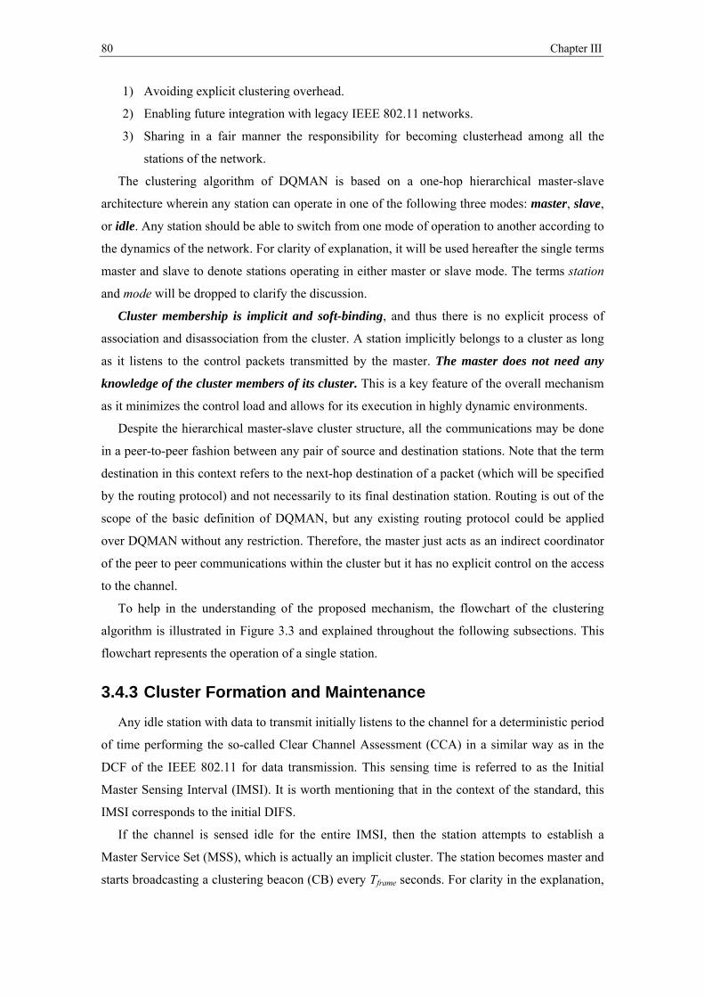
Chapter III
80
1) Avoiding explicit clustering overhead.
2) Enabling future integration with legacy IEEE 802.11 networks.
3) Sharing in a fair manner the responsibility for becoming clusterhead among all the
stations of the network.
The clustering algorithm of DQMAN is based on a one-hop hierarchical master-slave
architecture wherein any station can operate in one of the following three modes: master, slave,
or idle. Any station should be able to switch from one mode of operation to another according to
the dynamics of the network. For clarity of explanation, it will be used hereafter the single terms
master and slave to denote stations operating in either master or slave mode. The terms station
and mode will be dropped to clarify the discussion.
Cluster membership is implicit and soft-binding, and thus there is no explicit process of
association and disassociation from the cluster. A station implicitly belongs to a cluster as long
as it listens to the control packets transmitted by the master. The master does not need any
knowledge of the cluster members of its cluster. This is a key feature of the overall mechanism
as it minimizes the control load and allows for its execution in highly dynamic environments.
Despite the hierarchical master-slave cluster structure, all the communications may be done
in a peer-to-peer fashion between any pair of source and destination stations. Note that the term
destination in this context refers to the next-hop destination of a packet (which will be specified
by the routing protocol) and not necessarily to its final destination station. Routing is out of the
scope of the basic definition of DQMAN, but any existing routing protocol could be applied
over DQMAN without any restriction. Therefore, the master just acts as an indirect coordinator
of the peer to peer communications within the cluster but it has no explicit control on the access
to the channel.
To help in the understanding of the proposed mechanism, the flowchart of the clustering
algorithm is illustrated in Figure 3.3 and explained throughout the following subsections. This
flowchart represents the operation of a single station.
3.4.3 Cluster Formation and Maintenance
Any idle station with data to transmit initially listens to the channel for a deterministic period
of time performing the so-called Clear Channel Assessment (CCA) in a similar way as in the
DCF of the IEEE 802.11 for data transmission. This sensing time is referred to as the Initial
Master Sensing Interval (IMSI). It is worth mentioning that in the context of the standard, this
IMSI corresponds to the initial DIFS.
If the channel is sensed idle for the entire IMSI, then the station attempts to establish a
Master Service Set (MSS), which is actually an implicit cluster. The station becomes master and
starts broadcasting a clustering beacon (CB) every Tframe seconds. For clarity in the explanation,
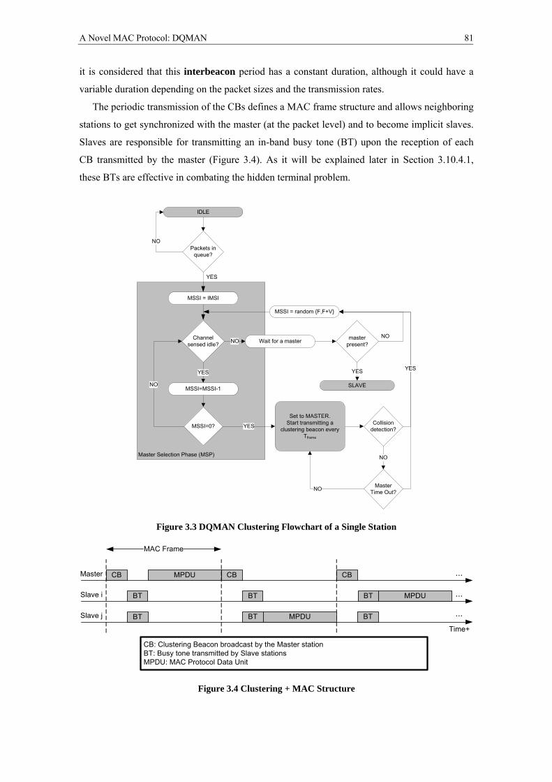
A Novel MAC Protocol: DQMAN
81
it is considered that this interbeacon period has a constant duration, although it could have a
variable duration depending on the packet sizes and the transmission rates.
The periodic transmission of the CBs defines a MAC frame structure and allows neighboring
stations to get synchronized with the master (at the packet level) and to become implicit slaves.
Slaves are responsible for transmitting an in-band busy tone (BT) upon the reception of each
CB transmitted by the master (Figure 3.4). As it will be explained later in Section 3.10.4.1,
these BTs are effective in combating the hidden terminal problem.
Master Selection Phase (MSP)
IDLE
Packets in queue?
NO
MSSI = random {F,F+V}
Channel sensed idle?
Wait for a masterNO
MSSI=MSSI-1
YES
MSSI=0?
NO
Set to MASTER. Start transmitting a
clustering beacon every Tframe
YESCollision
detection?
NO
Master Time Out?
NO
YES
master present?
SLAVE
YES
MSSI = IMSI
YES
NO
Figure 3.3 DQMAN Clustering Flowchart of a Single Station
CB CBMaster
Slave i
MPDU
MAC Frame
Slave j
CB
BT
BT
BT
BT
BT
BT
...
...
...MPDU
MPDU
Time+
CB: Clustering Beacon broadcast by the Master stationBT: Busy tone transmitted by Slave stationsMPDU: MAC Protocol Data Unit
Figure 3.4 Clustering + MAC Structure
Chapter III
82
In the case that all the stations of the network are in the transmission range of each other (no
hidden terminals) the IMSI can take the duration of a DIFS, as in the 802.11 Standard [9].
Otherwise, in general multi-hop settings with the potential presence of hidden terminals, this
IMSI should take the maximum time an active master will remain silent, which corresponds to
the time between consecutive BTs.
The BTs promote a minimum distance of three hops between masters and allow combating
the hidden terminal problem at the cost of increasing the exposed terminal problem. In addition,
the BTs constitute a collision detection mechanism for those stations which attempt to become
master. Note that if a recently set master does not sense any BT after the transmission of the
CB, this is because there are no slaves present in its neighborhood. Two situations may produce
this fact:
1) A collision has occurred with another station attempting to become master
simultaneously, or
2) It constitutes an isolated master with no other station in its vicinity.
In the case of success, the time elapsed between the BTs and the next CB is devoted to the
exchange of data and control packets. Any MAC protocol can be executed to control these
transmissions.
The MAC frame structure is illustrated in Figure 3.4. In this example, a station operating in
master mode transmits a CB every Tframe seconds. Upon the reception of the CB, the two
associated slave stations i and j transmit a BT. Finally, the time between BT and CB is used for
the transmission of data packets.
On the other hand, if an idle station senses the channel busy when attempting to get access to
it for the first time, or it collides when attempting to become master, it initiates a Master
Selection Phase (MSP). This phase consists in setting up a Master Selection Silent Interval
(MSSI) counter to a random value. This value must be within a MSSI window (measured in
time slots) according to the algorithm presented in the next section. This operation is similar to
the Binary Exponential Backoff of the IEEE 802.11 Standard.
Likewise, any station performing a MSP listens to the channel and decrements the MSSI
counter by one unit after each time slot as long as the channel is sensed idle. Upon the
expiration of the MSSI counter, the station attempts to establish its MSS (cluster). The
algorithm to set the initial value of the MSSI counter is presented in the following section.
3.4.4 Setting Up the Value of the MSSI
The MSSI selection algorithm is summarized in (3.1) where 1 and 0 are tunable
parameters and take integer values. Recall that the MSSI value represents the number of time
slots the channel will be sensed before attempting to set a MSS (cluster).
A Novel MAC Protocol: DQMAN
83
,
, where [0, 1].
FMSSI F V
V Uniform
(3.1)
Uniform[·] stands for a uniform integer random variable. As expressed in (3.1), the value of
the MSSI counter is the sum of two terms: F and V. F is a deterministic period of time and V is
a randomized value.
The purpose of the fixed minimum period of time F is to reduce the probability that a station
becomes master twice consecutively in time as it will be explained in Section 3.8.3.3.
On the other hand, the randomized time interval V is required to reduce the probability that
two or more stations try to become master simultaneously in the same area and collide. Since
the parameter defines the size of the uniform random contention window, its value should be
properly selected as a function of the number of active stations. A proper tuning of this
parameter avoids either unnecessary wasted time in deferral periods or a high probability of
collisions.
Despite this algorithm, collisions can still occur. The collision resolution algorithm of
DQMAN is described in the next section.
3.4.5 Master Collision Resolution
A collision occurs when two or more stations in the same transmission range attempt to
become master simultaneously and their CBs collide. Any station which attempts to establish its
MSS interprets that a collision with at least another station has occurred if no busy tones (BTs)
from other slaves are received after the transmission of the CB. Since the corresponding CBs
collide, the possible potential slaves are not able to receive them properly. The stations involved
in the collision reinitiate a new MSP by selecting a new value for their respective MSSI
counters as soon as the collision is detected.
It is worth mentioning that any backoff-based collision resolution algorithm could be used to
optimize the clustering process. However, since contention-based access in DQMAN is
confined to clustering phases, which last for less time than clustered phases, a simple algorithm
as the one described in the previous section is preferred.
3.4.6 Dynamic Reclustering
Any master reverts to idle mode whenever there are no more pending data transmissions
among all the stations associated to its MSS (including its data traffic). As it will be explained
later in Section 3.5, a master can easily learn whether there is no data activity in the network
using the MAC protocol rules and the state of the two distributed logical queues that manage
both the collision resolution and the transmission of data. Therefore, the cluster layout is
Chapter III
84
dynamically changed along time as a function of the aggregated traffic load offered to the
different sets of nodes in the network.
In addition, whenever a slave mishears a number of CBs from the master, it reverts to idle.
Note that this happens if the master has either moved away from the slave (or vice versa) or the
former has been switched off. It is worth mentioning that due to the variable channel fading, a
CB can be lost without implying that the connection with the master is permanently lost. For
these cases, it is convenient to consider that a master is not reachable if more than one CB is
lost. Without loss of generality, and unless otherwise stated, it will be henceforth considered
that a slave disassociates from the master if it mishears two consecutive CBs.
On the other hand, in order to avoid potential static cluster settings under heavy traffic
conditions, any master reverts to idle after a bounded period of time regardless of the waiting
data to be transmitted within its cluster. This is referred to as the Master Time Out (MTO)
mechanism; any master decrements its MTO counter by one unit after the transmission of each
CB, i.e., after each MAC frame. Upon expiration of the counter, the station always reverts to
idle mode regardless of the data activity of the network. The selection of the value of this
maximum time depends on the network application and it is out of the scope of the basic
definition of DQMAN. The MTO mechanism and the improvement attained in terms of fairness
in a single-hop network are presented in [14]. There, it is shown that, within that context, high
values of the MTO (long cluster life times) yield higher steady-state network throughput due to
the fact that more time is devoted to the execution of the high-performance MAC protocol
within each cluster and less time is devoted to contention-based clustering phases. However,
long cluster life times lead to unfairness in the responsibility of being master and promote the
creation of deadlocked stations in multi-hop networks, as will be further discussed in Section
3.10. Therefore, there is a tradeoff between maximum stable throughput (high values of the
MTO) and fairness (low values of the MTO).
3.5 The MAC Protocol
As aforementioned, the passive clustering approach of DQMAN can operate in conjunction
with any infrastructure-based MAC protocol. The particular approach presented in this thesis is
to use the near-optimum DQCA protocol within each cluster. The description and adaptation of
the DQCA protocol to operate together with the clustering of DQMAN is comprehensively
described throughout the following sections.
3.5.1 Description
Within the context of DQMAN, the clustering beacon (CB) described before gets the form
of a control packet, named Feedback Packet (FBP). This FBP can be seen as the CB with
additional control information necessary for the protocol operation. Therefore, the FBP is
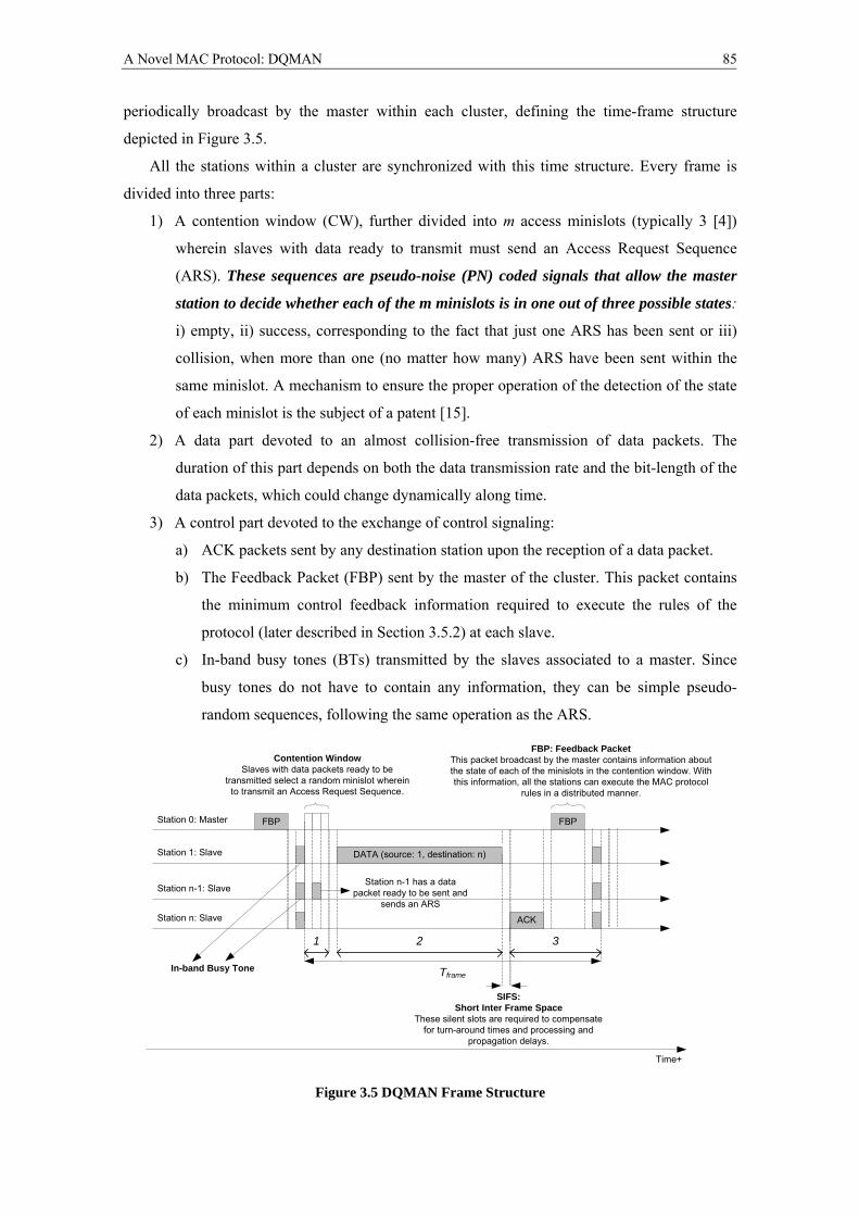
A Novel MAC Protocol: DQMAN
85
periodically broadcast by the master within each cluster, defining the time-frame structure
depicted in Figure 3.5.
All the stations within a cluster are synchronized with this time structure. Every frame is
divided into three parts:
1) A contention window (CW), further divided into m access minislots (typically 3 [4])
wherein slaves with data ready to transmit must send an Access Request Sequence
(ARS). These sequences are pseudo-noise (PN) coded signals that allow the master
station to decide whether each of the m minislots is in one out of three possible states:
i) empty, ii) success, corresponding to the fact that just one ARS has been sent or iii)
collision, when more than one (no matter how many) ARS have been sent within the
same minislot. A mechanism to ensure the proper operation of the detection of the state
of each minislot is the subject of a patent [15].
2) A data part devoted to an almost collision-free transmission of data packets. The
duration of this part depends on both the data transmission rate and the bit-length of the
data packets, which could change dynamically along time.
3) A control part devoted to the exchange of control signaling:
a) ACK packets sent by any destination station upon the reception of a data packet.
b) The Feedback Packet (FBP) sent by the master of the cluster. This packet contains
the minimum control feedback information required to execute the rules of the
protocol (later described in Section 3.5.2) at each slave.
c) In-band busy tones (BTs) transmitted by the slaves associated to a master. Since
busy tones do not have to contain any information, they can be simple pseudo-
random sequences, following the same operation as the ARS.
Tframe
Time+
Contention WindowSlaves with data packets ready to be
transmitted select a random minislot wherein to transmit an Access Request Sequence.
FBP: Feedback PacketThis packet broadcast by the master contains information about the state of each of the minislots in the contention window. With this information, all the stations can execute the MAC protocol
rules in a distributed manner.
In-band Busy Tone
Station 0: Master
Station 1: Slave
Station n: Slave
FBP
ACK
DATA (source: 1, destination: n)
FBP
Station n-1: SlaveStation n-1 has a data
packet ready to be sent and sends an ARS
SIFS: Short Inter Frame Space
These silent slots are required to compensate for turn-around times and processing and
propagation delays.
1 2 3
Figure 3.5 DQMAN Frame Structure
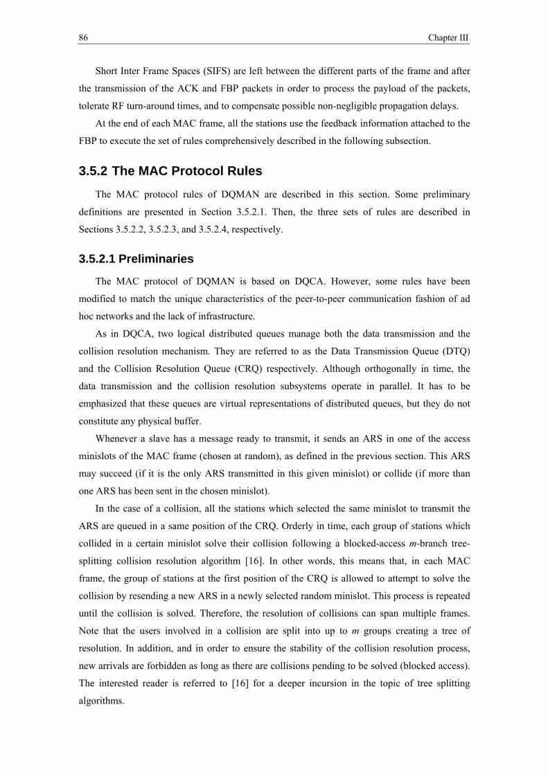
Chapter III
86
Short Inter Frame Spaces (SIFS) are left between the different parts of the frame and after
the transmission of the ACK and FBP packets in order to process the payload of the packets,
tolerate RF turn-around times, and to compensate possible non-negligible propagation delays.
At the end of each MAC frame, all the stations use the feedback information attached to the
FBP to execute the set of rules comprehensively described in the following subsection.
3.5.2 The MAC Protocol Rules
The MAC protocol rules of DQMAN are described in this section. Some preliminary
definitions are presented in Section 3.5.2.1. Then, the three sets of rules are described in
Sections 3.5.2.2, 3.5.2.3, and 3.5.2.4, respectively.
3.5.2.1 Preliminaries
The MAC protocol of DQMAN is based on DQCA. However, some rules have been
modified to match the unique characteristics of the peer-to-peer communication fashion of ad
hoc networks and the lack of infrastructure.
As in DQCA, two logical distributed queues manage both the data transmission and the
collision resolution mechanism. They are referred to as the Data Transmission Queue (DTQ)
and the Collision Resolution Queue (CRQ) respectively. Although orthogonally in time, the
data transmission and the collision resolution subsystems operate in parallel. It has to be
emphasized that these queues are virtual representations of distributed queues, but they do not
constitute any physical buffer.
Whenever a slave has a message ready to transmit, it sends an ARS in one of the access
minislots of the MAC frame (chosen at random), as defined in the previous section. This ARS
may succeed (if it is the only ARS transmitted in this given minislot) or collide (if more than
one ARS has been sent in the chosen minislot).
In the case of a collision, all the stations which selected the same minislot to transmit the
ARS are queued in a same position of the CRQ. Orderly in time, each group of stations which
collided in a certain minislot solve their collision following a blocked-access m-branch tree-
splitting collision resolution algorithm [16]. In other words, this means that, in each MAC
frame, the group of stations at the first position of the CRQ is allowed to attempt to solve the
collision by resending a new ARS in a newly selected random minislot. This process is repeated
until the collision is solved. Therefore, the resolution of collisions can span multiple frames.
Note that the users involved in a collision are split into up to m groups creating a tree of
resolution. In addition, and in order to ensure the stability of the collision resolution process,
new arrivals are forbidden as long as there are collisions pending to be solved (blocked access).
The interested reader is referred to [16] for a deeper incursion in the topic of tree splitting
algorithms.
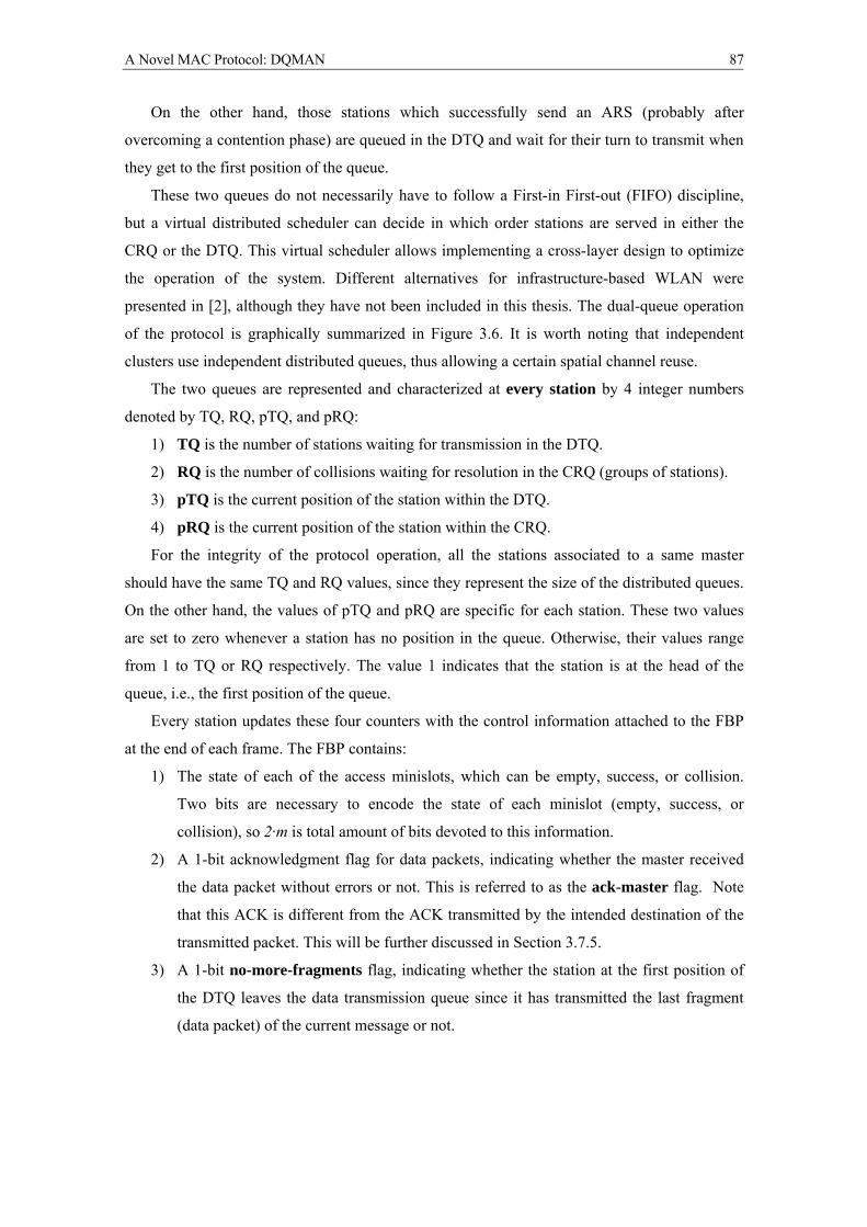
A Novel MAC Protocol: DQMAN
87
On the other hand, those stations which successfully send an ARS (probably after
overcoming a contention phase) are queued in the DTQ and wait for their turn to transmit when
they get to the first position of the queue.
These two queues do not necessarily have to follow a First-in First-out (FIFO) discipline,
but a virtual distributed scheduler can decide in which order stations are served in either the
CRQ or the DTQ. This virtual scheduler allows implementing a cross-layer design to optimize
the operation of the system. Different alternatives for infrastructure-based WLAN were
presented in [2], although they have not been included in this thesis. The dual-queue operation
of the protocol is graphically summarized in Figure 3.6. It is worth noting that independent
clusters use independent distributed queues, thus allowing a certain spatial channel reuse.
The two queues are represented and characterized at every station by 4 integer numbers
denoted by TQ, RQ, pTQ, and pRQ:
1) TQ is the number of stations waiting for transmission in the DTQ.
2) RQ is the number of collisions waiting for resolution in the CRQ (groups of stations).
3) pTQ is the current position of the station within the DTQ.
4) pRQ is the current position of the station within the CRQ.
For the integrity of the protocol operation, all the stations associated to a same master
should have the same TQ and RQ values, since they represent the size of the distributed queues.
On the other hand, the values of pTQ and pRQ are specific for each station. These two values
are set to zero whenever a station has no position in the queue. Otherwise, their values range
from 1 to TQ or RQ respectively. The value 1 indicates that the station is at the head of the
queue, i.e., the first position of the queue.
Every station updates these four counters with the control information attached to the FBP
at the end of each frame. The FBP contains:
1) The state of each of the access minislots, which can be empty, success, or collision.
Two bits are necessary to encode the state of each minislot (empty, success, or
collision), so 2·m is total amount of bits devoted to this information.
2) A 1-bit acknowledgment flag for data packets, indicating whether the master received
the data packet without errors or not. This is referred to as the ack-master flag. Note
that this ACK is different from the ACK transmitted by the intended destination of the
transmitted packet. This will be further discussed in Section 3.7.5.
3) A 1-bit no-more-fragments flag, indicating whether the station at the first position of
the DTQ leaves the data transmission queue since it has transmitted the last fragment
(data packet) of the current message or not.
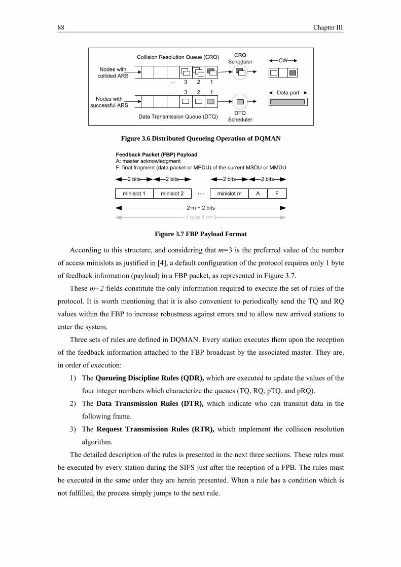
Chapter III
88
Collision Resolution Queue (CRQ)
Data Transmission Queue (DTQ)
Nodes with collided ARS
Nodes with successful ARS
CRQScheduler
DTQ Scheduler
CW
Data part2 13...
2 13...
Figure 3.6 Distributed Queueing Operation of DQMAN
minislot 1 minislot 2 minislot m FA
2 bits 2 bits 2 bits 2 bits
2·m + 2 bits
1 byte if m=3
Feedback Packet (FBP) PayloadA: master acknowledgmentF: final fragment (data packet or MPDU) of the current MSDU or MMDU
...
Figure 3.7 FBP Payload Format
According to this structure, and considering that m=3 is the preferred value of the number
of access minislots as justified in [4], a default configuration of the protocol requires only 1 byte
of feedback information (payload) in a FBP packet, as represented in Figure 3.7.
These m+2 fields constitute the only information required to execute the set of rules of the
protocol. It is worth mentioning that it is also convenient to periodically send the TQ and RQ
values within the FBP to increase robustness against errors and to allow new arrived stations to
enter the system.
Three sets of rules are defined in DQMAN. Every station executes them upon the reception
of the feedback information attached to the FBP broadcast by the associated master. They are,
in order of execution:
1) The Queueing Discipline Rules (QDR), which are executed to update the values of the
four integer numbers which characterize the queues (TQ, RQ, pTQ, and pRQ).
2) The Data Transmission Rules (DTR), which indicate who can transmit data in the
following frame.
3) The Request Transmission Rules (RTR), which implement the collision resolution
algorithm.
The detailed description of the rules is presented in the next three sections. These rules must
be executed by every station during the SIFS just after the reception of a FPB. The rules must
be executed in the same order they are herein presented. When a rule has a condition which is
not fulfilled, the process simply jumps to the next rule.
A Novel MAC Protocol: DQMAN
89
3.5.2.2 QDR (Queueing Discipline Rules)
1) Each station increases the value of TQ by one unit for each control minislot with the
‘successful’ state in the previous frame, indicating that a new station has entered the
DTQ.
2) The value of TQ is reduced by one unit if a data packet has just been successfully
transmitted and there are no more fragments to be transmitted. In this case, the
transmitting station leaves the queue.
3) If there are collisions pending to be resolved, which means that RQ>0, the value of RQ
is reduced by one unit. Those stations at the head of CRQ will try to resolve their
collision within the following frame by resending a new ARS in a newly selected access
minislot.
4) The value of RQ is incremented by one unit for each control minislot where an ARS
collision occurred in the previous frame. No matter the multiplicity of the collision
(which in fact is not necessary to be detected) just one unit per collision will be added
to RQ.
5) Each station calculates its own position in the queues (values for pTQ and pRQ)
depending on whether it has sent or not an ARS:
a) If the station has transmitted an ARS in a minislot and the state of that minislot is
“success” then the station sets its pTQ to the corresponding value at the end of the
DTQ. It should be mentioned that the events of the control minislots are sorted by a
time arrival criterion, meaning that a station with successful request at the first
control slot enters the data queue before a station whose request was sent at the
second control minislot. In the case the ARS has collided, the station calculates its
position among all the present collisions and sets pRQ to the corresponding value at
the end of the CRQ.
b) If the station has not sent any ARS, then pTQ and pRQ follow the same update
rules as TQ and RQ, respectively (rules 1 to 4), as long as their initial values are
non-zero.
c) Those stations which have successfully transmitted the last fragment of a message
to the intended destination and have correctly received the corresponding ACK,
even if they have not received acknowledgement from the master, reduce their pTQ
value in one unit, and thus leave the DTQ.
3.5.2.3 DTR (Data Transmission Rules)
1) If TQ, RQ, pTQ, and pRQ are all equal to 0, every station with a message ready to be
sent transmits the first packet of the message in the data part. This rule is referred to as
Chapter III
90
the immediate access rule, and it constitutes the only possible cause of a collision in
the data part. However, it avoids an unnecessary empty data frame and improves the
packet transmission delay when the traffic load is low and thus the probability of having
a collision is also low.
2) If pTQ=1, the station is allowed to transmit a packet in the following frame. If this
packet is the last fragment of a message, it should indicate it in the header of the data
packet so that the master can set the no-more-fragments flag in the next FBP. This will
let the next station in the DTQ to transmit in the following frame.
3.5.2.4 RTR (Request Transmission Rules)
1) If RQ, pTQ, and pRQ are all equal to 0, every station with a message ready to be
transmitted, randomly selects one out of the m control minislots and transmits an ARS
in the following frame.
2) If a master, according to the prior rule, is about to transmit an ARS in the following
frame, instead of actually transmitting an ARS, it reports a successful minislot in the
first empty minislot of the following frame. Besides saving the energy of transmitting
an ARS, collisions involving the master station are completely avoided. In the case of
sensing all the minislots busy, it postpones the ARS success notification to the first
frame with at least one empty minislot.
3) If pRQ=1, the station randomly selects one out of the m control minislots and transmits
an ARS within it in order to try to resolve the collision in the following frame.
3.6 Example of Operation
In order to clarify how both the clustering and the MAC protocols are smoothly integrated
with each other, an example of operation is illustrated in Figure 3.8, and described in this
section. Although there are many combinations that may occur, the most representative cases
have been exemplified in this section in order to facilitate the understanding of the protocol
operation.
Two stations, namely M1 and M2, have established their independent MSS (clusters). These
stations periodically send the beacons FBP1 and FBP2, respectively, defining a time frame
structure which allows stations S1 to S5 to get synchronized to their closest master station and
to become slave stations. S1, S2 and S3 get synchronized with M2, while S4 and S5 get
synchronized with M1. Accordingly, all these slave stations transmit a BT after the reception of
each FBP. To simplify the example, a configuration with only two access minislots is
considered.
As it can be seen in Figure 3.8, the frames at both MSS run independently of each other.
DTQ-1 and CRQ-1 are the queues at the MSS coordinated by M1, and DTQ-2 and CRQ-2 are
A Novel MAC Protocol: DQMAN
91
the queues at the MSS coordinated by M2. TQ-1, RQ-1, TQ-2 and RQ-2 are the total number of
positions occupied in either the DTQ or the CRQ of MSS of M1 and the MSS of M2,
respectively.
First, the focus is on the MSS of M2, and the sequence of events in chronological order is:
1) Frame i-1 (not shown in the figure): S1 sends an ARS because it has data to transmit.
Upon the reception of the FBP2 at the end of the frame, S1 is aware of the successful
request and gets the first position of DTQ-2, i.e., pTQs1=1. S1 will transmit data in
frame i.
2) Frame i: S1 transmits a data packet to S2. S2 acknowledges the reception of the data
packet by broadcasting an ACK. S1 leaves the DTQ-2. In addition, S2 and S3 have data
packets ready to transmit and they randomly select an access minislot to send an access
request (ARS). In this example, S2 selects minislot 2 and S3 selects minislot 1.
Therefore, there are no collisions and they succeed in their access request. Upon the
reception of the FBP2 at the end of frame i, S2 and S3 get the positions 2 and 1,
respectively, in DTQ-2. Therefore, TQ-2=2, pTQS2=2, and pTQS3=1. Consequently, S3
will transmit data in frame i+1.
3) Frame i+1: S3 transmits data to S2. S2 acknowledges the reception of the data packet
with an ACK. Therefore, S3 leaves the DTQ-2. On the other hand, S1 has data to
transmit and selects a minislot at random to send an ARS. Upon the reception of the
FBP2 at the end of frame i, S1 is aware of the successful request and enters the DTQ-2
at the third position, i.e., pTQS1=3. Why not at the second position if no more ARS have
been sent in this frame? According to the protocol rule RTR-2, master stations avoid
contention and thus although M2 has not sent an actual ARS, it reports in the FBP2 a
successful ARS in the first empty minislot (minislot 1) since it has data to transmit.
Consequently, M2 gets the second position in DTQ-2. Summarizing, at the end of frame
i+1 TQ-2=3, pTQS1=3, pTQM2=2, and pTQS2=1.
4) Frame i+2: S2 transmits data.
As it has been shown in this first example, no collisions have occurred and thus the CRQ-2
has remained empty for the whole operation. However, let us look at the MSS established by
M1. Once again, events are explained in chronological order, but with a different time reference
(recall that clusters are not synchronized with each other, and thus i j ):
1) Frame j-1 (not shown in the figure): The system is empty and thus TQ-1=0 and RQ-
1=0. No ARSs are sent.
2) Frame j: Both stations S4 and S5 have data packets in the buffers. They select an
access minislot at random. The two stations select minislot 2 and thus they collide.
Upon the reception of the FBP1 at the end of the frame, they are aware of the collision
and they both enter the first position of the CRQ-1, i.e., RQ-1=1 and pRQS4=pRQS5=1.
Chapter III
92
Note that both S4 and S5 occupy the same position in the queue. In the case that another
pair of stations had collided in a different minislot they would occupy another position
in CRQ-1. This is the key concept behind tree-splitting algorithms; collisions are
resolved separately, forming a tree of resolutions.
3) Frame j+1: Stations S4 and S5 occupy the first position of the CRQ-1, and thus they
attempt to solve their collision. They leave the CRQ-1 by updating their value of pRQS4
and pRQS5 to 0. Both stations reselect access minislot at random. In this case, S4 selects
minislot 1 and S5 selects minislot 2. Therefore, at the reception of the FBP1 at the end
of the frame, they get to the positions 1 and 2 of DTQ-1, respectively. In addition, M1
reports a successful ARS in minislot 3 to transmit its own data. In summary, at the end
of the frame, TQ-1=3, pTQM1=3, pTQS4=2, and pTQS5=1. On the other hand, RQ-1=0
(there are no collisions pending to be solved).
4) Frame j+2: S5 transmits data.
3.7 General Discussion
In this section, some special features of DQMAN are described. They should be considered
for a proper implementation of the protocol in actual hardware. They have not been included in
the basic definition of the protocol presented in the previous section in order to clarify the basic
operation of the protocol.
3.7.1 Special Rule: Initialization of a Cluster
Considering the rules presented in Section 3.5.2, it has to be mentioned that upon
initialization of a cluster, the master indicates in the very first FBP the values of TQ=1 and
RQ=0.
These values indicate that the master initially has the first position in the data transmission
queue and also that new access requests are allowed for those stations with data to transmit as
well. Accordingly, the master sets its pTQ=1 to transmit in the very next MAC frame.
Note that this operation corresponds to a special kind of immediate access rule for the
master which is free of collisions.
3.7.2 Avoiding Empty Data Frames
The master is aware of the state of the access minislots since it is one hop away from all
slaves. Therefore, it can avoid the occurrence of empty data frames under low data traffic loads
in the following cases:
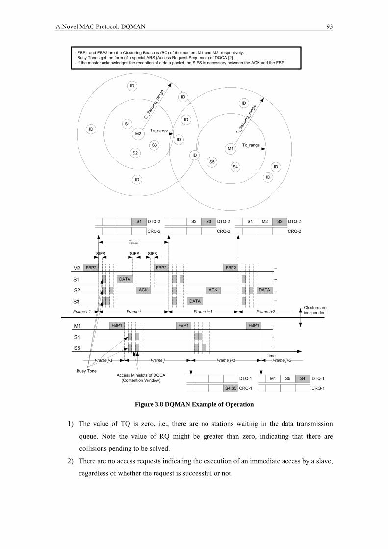
A Novel MAC Protocol: DQMAN
93
DATA
ACKACK
FBP2
FBP1
FBP2
M2Tx_range
C_S
ensi
ng_r
ange
S1
S2
S3
ID
ID
ID
ID
ID
M1Tx_range
C_S
ensi
ng_r
ange
S5S4
ID
ID
ID
ID
ID
DATA
FBP2
FBP1
Busy Tone
Tframe
...
...
...
...
...
...
...
time
Clusters are independent
FBP1M1
S4
S5
M2
S1
S2
S3
Access Minislots of DQCA(Contention Window)
SIFS SIFS
- FBP1 and FBP2 are the Clustering Beacons (BC) of the masters M1 and M2, respectively. - Busy Tones get the form of a special ARS (Access Request Sequence) of DQCA [2]. - If the master acknowledges the reception of a data packet, no SIFS is necessary between the ACK and the FBP
DATA
SIFS
S4,S5
DTQ-1
CRQ-1
M1 S5 S4 DTQ-1
CRQ-1
S2 S3 S1 M2 S2S1 DTQ-2
CRQ-2
Frame i Frame i+1 Frame i+2
Frame j Frame j+1
DTQ-2
CRQ-2
DTQ-2
CRQ-2
Frame i-1
Frame j-1 Frame j+2
Figure 3.8 DQMAN Example of Operation
1) The value of TQ is zero, i.e., there are no stations waiting in the data transmission
queue. Note the value of RQ might be greater than zero, indicating that there are
collisions pending to be solved.
2) There are no access requests indicating the execution of an immediate access by a slave,
regardless of whether the request is successful or not.
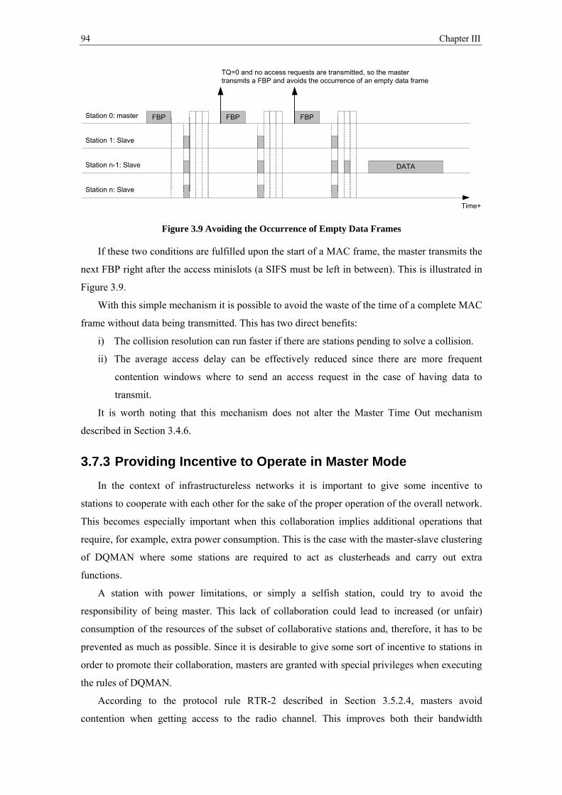
Chapter III
94
Station 0: master
Station 1: Slave
Station n: Slave
FBPFBP
Station n-1: Slave
FBP
DATA
Time+
TQ=0 and no access requests are transmitted, so the master transmits a FBP and avoids the occurrence of an empty data frame
Figure 3.9 Avoiding the Occurrence of Empty Data Frames
If these two conditions are fulfilled upon the start of a MAC frame, the master transmits the
next FBP right after the access minislots (a SIFS must be left in between). This is illustrated in
Figure 3.9.
With this simple mechanism it is possible to avoid the waste of the time of a complete MAC
frame without data being transmitted. This has two direct benefits:
i) The collision resolution can run faster if there are stations pending to solve a collision.
ii) The average access delay can be effectively reduced since there are more frequent
contention windows where to send an access request in the case of having data to
transmit.
It is worth noting that this mechanism does not alter the Master Time Out mechanism
described in Section 3.4.6.
3.7.3 Providing Incentive to Operate in Master Mode
In the context of infrastructureless networks it is important to give some incentive to
stations to cooperate with each other for the sake of the proper operation of the overall network.
This becomes especially important when this collaboration implies additional operations that
require, for example, extra power consumption. This is the case with the master-slave clustering
of DQMAN where some stations are required to act as clusterheads and carry out extra
functions.
A station with power limitations, or simply a selfish station, could try to avoid the
responsibility of being master. This lack of collaboration could lead to increased (or unfair)
consumption of the resources of the subset of collaborative stations and, therefore, it has to be
prevented as much as possible. Since it is desirable to give some sort of incentive to stations in
order to promote their collaboration, masters are granted with special privileges when executing
the rules of DQMAN.
According to the protocol rule RTR-2 described in Section 3.5.2.4, masters avoid
contention when getting access to the radio channel. This improves both their bandwidth
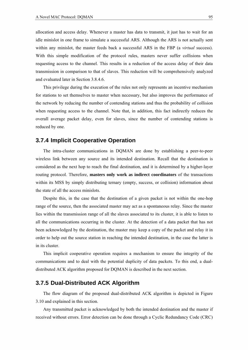
A Novel MAC Protocol: DQMAN
95
allocation and access delay. Whenever a master has data to transmit, it just has to wait for an
idle minislot in one frame to simulate a successful ARS. Although the ARS is not actually sent
within any minislot, the master feeds back a successful ARS in the FBP (a virtual success).
With this simple modification of the protocol rules, masters never suffer collisions when
requesting access to the channel. This results in a reduction of the access delay of their data
transmission in comparison to that of slaves. This reduction will be comprehensively analyzed
and evaluated later in Section 3.8.4.6.
This privilege during the execution of the rules not only represents an incentive mechanism
for stations to set themselves to master when necessary, but also improves the performance of
the network by reducing the number of contending stations and thus the probability of collision
when requesting access to the channel. Note that, in addition, this fact indirectly reduces the
overall average packet delay, even for slaves, since the number of contending stations is
reduced by one.
3.7.4 Implicit Cooperative Operation
The intra-cluster communications in DQMAN are done by establishing a peer-to-peer
wireless link between any source and its intended destination. Recall that the destination is
considered as the next hop to reach the final destination, and it is determined by a higher-layer
routing protocol. Therefore, masters only work as indirect coordinators of the transactions
within its MSS by simply distributing ternary (empty, success, or collision) information about
the state of all the access minislots.
Despite this, in the case that the destination of a given packet is not within the one-hop
range of the source, then the associated master may act as a spontaneous relay. Since the master
lies within the transmission range of all the slaves associated to its cluster, it is able to listen to
all the communications occurring in the cluster. At the detection of a data packet that has not
been acknowledged by the destination, the master may keep a copy of the packet and relay it in
order to help out the source station in reaching the intended destination, in the case the latter is
in its cluster.
This implicit cooperative operation requires a mechanism to ensure the integrity of the
communications and to deal with the potential duplicity of data packets. To this end, a dual-
distributed ACK algorithm proposed for DQMAN is described in the next section.
3.7.5 Dual-Distributed ACK Algorithm
The flow diagram of the proposed dual-distributed ACK algorithm is depicted in Figure
3.10 and explained in this section.
Any transmitted packet is acknowledged by both the intended destination and the master if
received without errors. Error detection can be done through a Cyclic Redundancy Code (CRC)
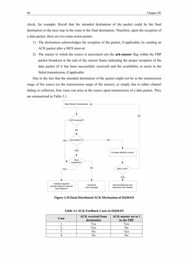
Chapter III
96
check, for example. Recall that the intended destination of the packet could be the final
destination or the next step in the route to the final destination. Therefore, upon the reception of
a data packet, there are two main action points:
1) The destination acknowledges the reception of the packet, if applicable, by sending an
ACK packet after a SIFS interval.
2) The master to which the source is associated sets the ack-master flag within the FBP
packet broadcast at the end of the current frame indicating the proper reception of the
data packet (if it has been successfully received) and the availability to assist in the
failed transmission, if applicable.
Due to the fact that the intended destination of the packet might not be in the transmission
range of the source (or the transmission range of the master), or simply due to either channel
fading or collisions, four cases can arise at the source upon transmission of a data packet. They
are summarized in Table 3.1.
Data Packet Transmission
ACK received?
ack-master=1?YES
NO
YES
More fragments?
Validate fragmentand get ready to transmit
next fragment
YES
Schedule next message
NO
Increase attempt counter
NO
MAX_tries?
Discard fragment and dissociate from Master
YES
NO
Figure 3.10 Dual-Distributed ACK Mechanism of DQMAN
Table 3.1 ACK Feedback Cases in DQMAN
Case ACK received from
destination ACK-master set to 1
in the FBP 1 Yes Yes 2 Yes No 3 No Yes 4 No No
A Novel MAC Protocol: DQMAN
97
In cases 1 and 2, the current packet is acknowledged by the destination indicating the
success in the transmission and, therefore, the next packet can be processed.
In case 3, the data packet will be relayed by the master. If the master is the transmitting
station and no ACK is received from the destination, then the transmission of the packet is
postponed.
In case 4, the source disassociates from the current master and resets to idle. Note that
considering the impairments of the wireless channel, this disassociation should be done only
after the consecutive occurrence of case 4.
3.8 Performance Analysis in Single-Hop Networks
3.8.1 Introduction
The performance of DQMAN in single-hop networks is theoretically analyzed in this
section. An infrastructureless wireless network formed by n stations is considered, all of them
within the transmission range of each other. They are uniformly distributed in the space. The
stations can move with any general unspecified mobility pattern as long as the previous
condition is maintained.
The analysis presented in this section is divided in two parts. First, the saturation throughput
of the protocol is evaluated in Section 3.8.3. Then, the model is generalized to arbitrary non-
saturated traffic loads in Section 3.8.4. This last model allows computing the throughput of
DQMAN, the average message transmission delay, and the average time a station operates in
each of the modes of operation (idle, master, or slave).
Before diving into the details of both models for saturation and non-saturation traffic
conditions, some preliminary definitions are given in the next section.
3.8.2 Preliminary Considerations and Definitions
Some preliminary considerations regarding the transmission rates, the channel error model,
and the time references are provided in Sections 3.8.2.1 and 3.8.2.2, respectively. The
throughput and average transmission delay are defined in Sections 3.8.2.3 and 3.8.2.4,
respectively.
3.8.2.1 Transmission Rates and Channel Error Model
The same model as the one considered in [17]-[22] is used in this analysis. Two common
and constant transmission rates are considered for all the stations depending on the type of
transmissions:
1) Control packets are transmitted at the lowest available transmission rate (most robust
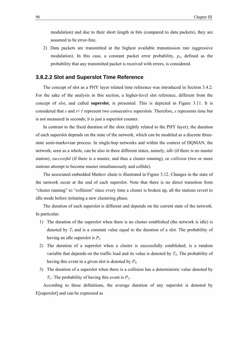
Chapter III
98
modulation) and due to their short length in bits (compared to data packets), they are
assumed to be error-free.
2) Data packets are transmitted at the highest available transmission rate (aggressive
modulation). In this case, a constant packet error probability, pe, defined as the
probability that any transmitted packet is received with errors, is considered.
3.8.2.2 Slot and Superslot Time Reference
The concept of slot as a PHY layer related time reference was introduced in Section 3.4.2.
For the sake of the analysis in this section, a higher-level slot reference, different from the
concept of slot, and called superslot, is presented. This is depicted in Figure 3.11. It is
considered that s and s+1 represent two consecutive superslots. Therefore, s represents time but
is not measured in seconds; it is just a superslot counter.
In contrast to the fixed duration of the slots (tightly related to the PHY layer), the duration
of each superslot depends on the state of the network, which can be modeled as a discrete three-
state semi-markovian process. In single-hop networks and within the context of DQMAN, the
network, seen as a whole, can be also in three different states, namely, idle (if there is no master
station), successful (if there is a master, and thus a cluster running), or collision (two or more
stations attempt to become master simultaneously and collide).
The associated embedded Markov chain is illustrated in Figure 3.12. Changes in the state of
the network occur at the end of each superslot. Note that there is no direct transition from
“cluster running” to “collision” since every time a cluster is broken up, all the stations revert to
idle mode before initiating a new clustering phase.
The duration of each superslot is different and depends on the current state of the network.
In particular:
1) The duration of the superslot when there is no cluster established (the network is idle) is
denoted by TI and is a constant value equal to the duration of a slot. The probability of
having an idle superslot is PI.
2) The duration of a superslot when a cluster is successfully established, is a random
variable that depends on the traffic load and its value is denoted by TS. The probability of
having this event in a given slot is denoted by PS.
3) The duration of a superslot when there is a collision has a deterministic value denoted by
TC. The probability of having this event is PC.
According to these definitions, the average duration of any superslot is denoted by
E[superslot] and can be expressed as
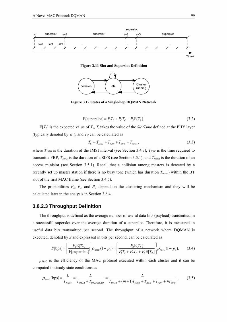
A Novel MAC Protocol: DQMAN
99
Time+
superslot superslot
superslot
superslot
slot slot slot ... ... ...
s s+1 s+2 s+3
Figure 3.11 Slot and Superslot Definition
idlecollisionCluster running
Figure 3.12 States of a Single-hop DQMAN Network
E[superslot] E[ ].I I C C S SPT P T P T (3.2)
E[TS] is the expected value of TS, TI takes the value of the SlotTime defined at the PHY layer
(typically denoted by ), and TC can be calculated as
,C IMSI FBP SIFS mslotT T T T T (3.3)
where TIMSI is the duration of the IMSI interval (see Section 3.4.3), TFBP is the time required to
transmit a FBP, TSIFS is the duration of a SIFS (see Section 3.5.1), and Tmslot is the duration of an
access minislot (see Section 3.5.1). Recall that a collision among masters is detected by a
recently set up master station if there is no busy tone (which has duration Tmslot) within the BT
slot of the first MAC frame (see Section 3.4.5).
The probabilities PS, PI, and PC depend on the clustering mechanism and they will be
calculated later in the analysis in Section 3.8.4.
3.8.2.3 Throughput Definition
The throughput is defined as the average number of useful data bits (payload) transmitted in
a successful superslot over the average duration of a superslot. Therefore, it is measured in
useful data bits transmitted per second. The throughput of a network where DQMAN is
executed, denoted by S and expressed in bits per second, can be calculated as
E[ ] E[ ]
[bps] (1 ) (1 ).E[superslot] E[ ]
S S S SMAC e MAC e
I I C C S S
P T P TS p p
PT P T P T
(3.4)
ρMAC is the efficiency of the MAC protocol executed within each cluster and it can be
computed in steady state conditions as
[bps] .( 1) 4MAC
frame DATA OVERHEAD DATA mslot ACK FBP SIFS
L L L
T T T T m T T T T
(3.5)
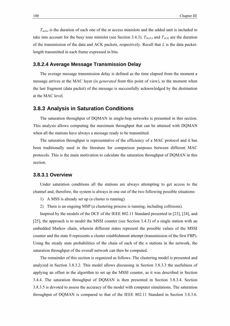
Chapter III
100
Tmslot is the duration of each one of the m access minislots and the added unit is included to
take into account for the busy tone minislot (see Section 3.4.3). TDATA and TACK are the duration
of the transmission of the data and ACK packets, respectively. Recall that L is the data packet-
length transmitted in each frame expressed in bits.
3.8.2.4 Average Message Transmission Delay
The average message transmission delay is defined as the time elapsed from the moment a
message arrives at the MAC layer (is generated from this point of view), to the moment when
the last fragment (data packet) of the message is successfully acknowledged by the destination
at the MAC level.
3.8.3 Analysis in Saturation Conditions
The saturation throughput of DQMAN in single-hop networks is presented in this section.
This analysis allows computing the maximum throughput that can be attained with DQMAN
when all the stations have always a message ready to be transmitted.
The saturation throughput is representative of the efficiency of a MAC protocol and it has
been traditionally used in the literature for comparison purposes between different MAC
protocols. This is the main motivation to calculate the saturation throughput of DQMAN in this
section.
3.8.3.1 Overview
Under saturation conditions all the stations are always attempting to get access to the
channel and, therefore, the system is always in one out of the two following possible situations:
1) A MSS is already set up (a cluster is running).
2) There is an ongoing MSP (a clustering process is running, including collisions).
Inspired by the models of the DCF of the IEEE 802.11 Standard presented in [23], [24], and
[25], the approach is to model the MSSI counter (see Section 3.4.3) of a single station with an
embedded Markov chain, wherein different states represent the possible values of the MSSI
counter and the state 0 represents a cluster establishment attempt (transmission of the first FBP).
Using the steady state probabilities of the chain of each of the n stations in the network, the
saturation throughput of the overall network can then be computed.
The remainder of this section is organized as follows. The clustering model is presented and
analyzed in Section 3.8.3.2. This model allows discussing in Section 3.8.3.3 the usefulness of
applying an offset in the algorithm to set up the MSSI counter, as it was described in Section
3.4.4. The saturation throughput of DQMAN is then presented in Section 3.8.3.4. Section
3.8.3.5 is devoted to assess the accuracy of the model with computer simulations. The saturation
throughput of DQMAN is compared to that of the IEEE 802.11 Standard in Section 3.8.3.6.
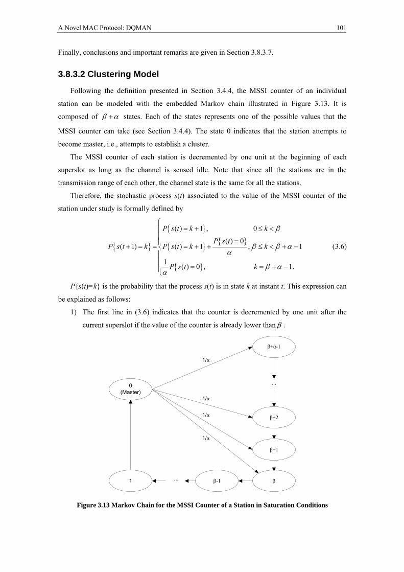
A Novel MAC Protocol: DQMAN
101
Finally, conclusions and important remarks are given in Section 3.8.3.7.
3.8.3.2 Clustering Model
Following the definition presented in Section 3.4.4, the MSSI counter of an individual
station can be modeled with the embedded Markov chain illustrated in Figure 3.13. It is
composed of states. Each of the states represents one of the possible values that the
MSSI counter can take (see Section 3.4.4). The state 0 indicates that the station attempts to
become master, i.e., attempts to establish a cluster.
The MSSI counter of each station is decremented by one unit at the beginning of each
superslot as long as the channel is sensed idle. Note that since all the stations are in the
transmission range of each other, the channel state is the same for all the stations.
Therefore, the stochastic process s(t) associated to the value of the MSSI counter of the
station under study is formally defined by
( ) 1 , 0
( ) 0( 1) ( ) 1 , 1
1( ) 0 , 1.
P s t k k
P s tP s t k P s t k k
P s t k
(3.6)
P{s(t)=k} is the probability that the process s(t) is in state k at instant t. This expression can
be explained as follows:
1) The first line in (3.6) indicates that the counter is decremented by one unit after the
current superslot if the value of the counter is already lower than .
β+1
β+2
β+α-1
...
β-1 β1 ...
0(Master)
1/α
1/α
1/α
1/α
Figure 3.13 Markov Chain for the MSSI Counter of a Station in Saturation Conditions
Chapter III
102
2) The second line in (3.6) indicates that the counter takes a value within [ , 1) if
either the counter is decremented after the current superslot or a clustering attempt has
been done in the previous superslot and the MSSI counter has been reinitiated at this
value with probability 1/ .
3) The third line in (3.6) indicates that the state 1k is only reached if a
clustering attempt has occurred in the previous superslot and the MSSI counter is
reinitialized at this value with probability 1/ .
Therefore, the analysis of the chain in steady state conditions can be done as follows. The
time dependency can be dropped in steady state conditions, and thus it is possible to adopt the
following short notation
lim { ( ) } .kt
P s t k P
(3.7)
Taking into account the MSSI counter operation, it is possible to write that
0 1 2 3 1... .P P P P P P (3.8)
This corresponds to the part of the chain corresponding to the fixed time period of the
MSSI. On the other hand, and according to the balance equations, it is possible to write that for
k ,
0 1
0
/ , 1
/ , 1.k
k
P P kP
P k
(3.9)
Iteratively, it is straightforward to derive that for k ,
0( ) .k
PP k
(3.10)
According to the Total Probability Theorem all probabilities must sum to one,
i.e.,1
0
1kk
P
, and thus it is possible to write that
1
00
1
( 1) ( ) 1.k
PP k
(3.11)
Developing this equation and using j k , it can be written that
10
01
00 0
( 1) ( )
11 1 1 1.
2
j
PP j
PP P
(3.12)
Finally, the probability that a station attempts to become master in a given superslot can be
expressed as
0
2.
2 1P
(3.13)
A Novel MAC Protocol: DQMAN
103
Therefore, the steady state probabilities of the chain are given by
2,
2 1
( ) 2, < 1.
2 1
k
0 k
Pk
k
(3.14)
The knowledge of these probabilities allows computing the saturation throughput of the
network and also justifying the usefulness of using a MSSI counter with an offset F. This
discussion is presented in the next section, while the calculation of the saturation throughput is
presented later in Section 3.8.3.4.
3.8.3.3 MSSI Counter with Offset: Master Sharing
By adding an offset to the MSSI counter (the fixed value F in (3.1) in Section 3.4.4), the
probability that a station is set to master twice consecutively is reduced. Therefore, the
responsibility of becoming master is shared in a fairer manner (in the short-term) among the
stations of the network. It is worth mentioning that the distributed operation of the clustering
algorithm and the fact that all the stations use the same size of the MSSI window ensures long-
term fairness in the access to the channel when attempting to establish a cluster.
After attempting to become master, a station sets up its MSSI counter to a value within the
interval [ , 1] . The probability that this station does not become master again when the
current MSS is broken up is denoted by PN and it can be computed as the sum of the probability
of two complementary events:
1. At least one of the other n–1 stations of the network has its MSSI counter within the
interval (0, ) .
2. The rest of the stations have their MSSI counter within the range [ , 1] and the
MSSI counter of the previous master has not the smallest value among all the MSSI
counters.
Then, considering that all the stations execute the protocol rules independently of each
other, this probability can be expressed as
1 1 11 (1 ) (1 ) ,n n
N
nP P P
n
(3.15)
where P is the probability for a single station to have its MSSI counter within the interval
(0, ) . Assuming that all the states in the MSP have the same steady state probability, it can be
computed as
.P
(3.16)
According to that, expression (3.15) rewrites as
Chapter III
104
1
11 1 .
n
NPn
(3.17)
The value of PN as a function of the number of stations (n) is depicted in Figure 3.14 for
different values of F. The curves have been obtained for different values of F (in particular
0, 10, 20, and 30) and for 64 . It is worth seeing that the bigger the value of F, the higher
the probability of not being in master mode in two consecutive MSS. On the other hand, the
higher the value of F, the more time latency is added to the transmission under low traffic
conditions.
Therefore, the proper selection of the value for F should take into account higher layer
requirements, especially involving fairness and energy consumption balance, and regarding the
packet transmission delay.
The saturation throughput of DQMAN is derived in the next section.
3.8.3.4 Saturation Throughput Analysis
In order to compute the saturation throughput of DQMAN expressed in (3.4) it is necessary
to calculate the expected duration of a superslot, as defined in (3.2). Recall that this expression
depends on:
1) The value of the parameters PS, PI, and PC, i.e., the probabilities that a superslot is
successful (a MSS is running), is idle (including the case when a clustering phase is
running), or a collision occurs (two or more stations attempt to become master
simultaneously), respectively.
2) The value of E[TS], i.e., the average duration of a successful superslot wherein a MSS is
running.
3) The values of TI and TC, which are the duration of idle and collided superslots,
respectively, and which have deterministic values as defined in Section 3.8.2.2.
Under saturation conditions, the duration of a successful slot is not a random variable, but
has a deterministic value, i.e., E[TS]=TS. This value corresponds the maximum time that a
master is allowed to operate as such without interruption, denoted by TMTO, plus the duration of
the initial channel sensing interval, and thus
E[ ] .S S IMSI MTOT T T T (3.18)
On the other hand, the probabilities PS, PI, and PC can be expressed as a function of both the
probability that a single station attempts to set up itself to master mode in a given superslot as
expressed in (3.13) and the total number of stations n.
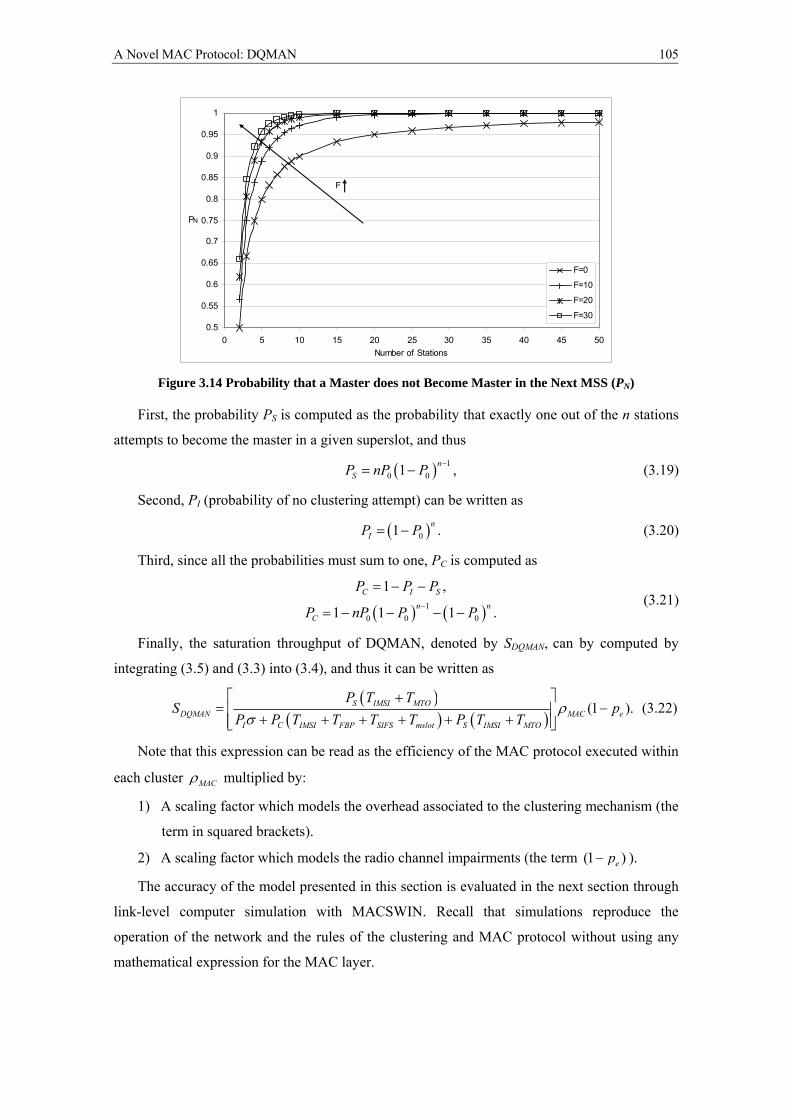
A Novel MAC Protocol: DQMAN
105
0.5
0.55
0.6
0.65
0.7
0.75
0.8
0.85
0.9
0.95
1
0 5 10 15 20 25 30 35 40 45 50
Number of Stations
PN
F=0
F=10
F=20
F=30
F
Figure 3.14 Probability that a Master does not Become Master in the Next MSS (PN)
First, the probability PS is computed as the probability that exactly one out of the n stations
attempts to become the master in a given superslot, and thus
1
0 01 ,n
SP nP P (3.19)
Second, PI (probability of no clustering attempt) can be written as
01 .n
IP P (3.20)
Third, since all the probabilities must sum to one, PC is computed as
1
0 0 0
1 ,
1 1 1 .
C I S
n n
C
P P P
P nP P P
(3.21)
Finally, the saturation throughput of DQMAN, denoted by SDQMAN, can by computed by
integrating (3.5) and (3.3) into (3.4), and thus it can be written as
(1 ).S IMSI MTO
DQMAN MAC eI C IMSI FBP SIFS mslot S IMSI MTO
P T TS p
P P T T T T P T T
(3.22)
Note that this expression can be read as the efficiency of the MAC protocol executed within
each cluster MAC multiplied by:
1) A scaling factor which models the overhead associated to the clustering mechanism (the
term in squared brackets).
2) A scaling factor which models the radio channel impairments (the term (1 )ep ).
The accuracy of the model presented in this section is evaluated in the next section through
link-level computer simulation with MACSWIN. Recall that simulations reproduce the
operation of the network and the rules of the clustering and MAC protocol without using any
mathematical expression for the MAC layer.
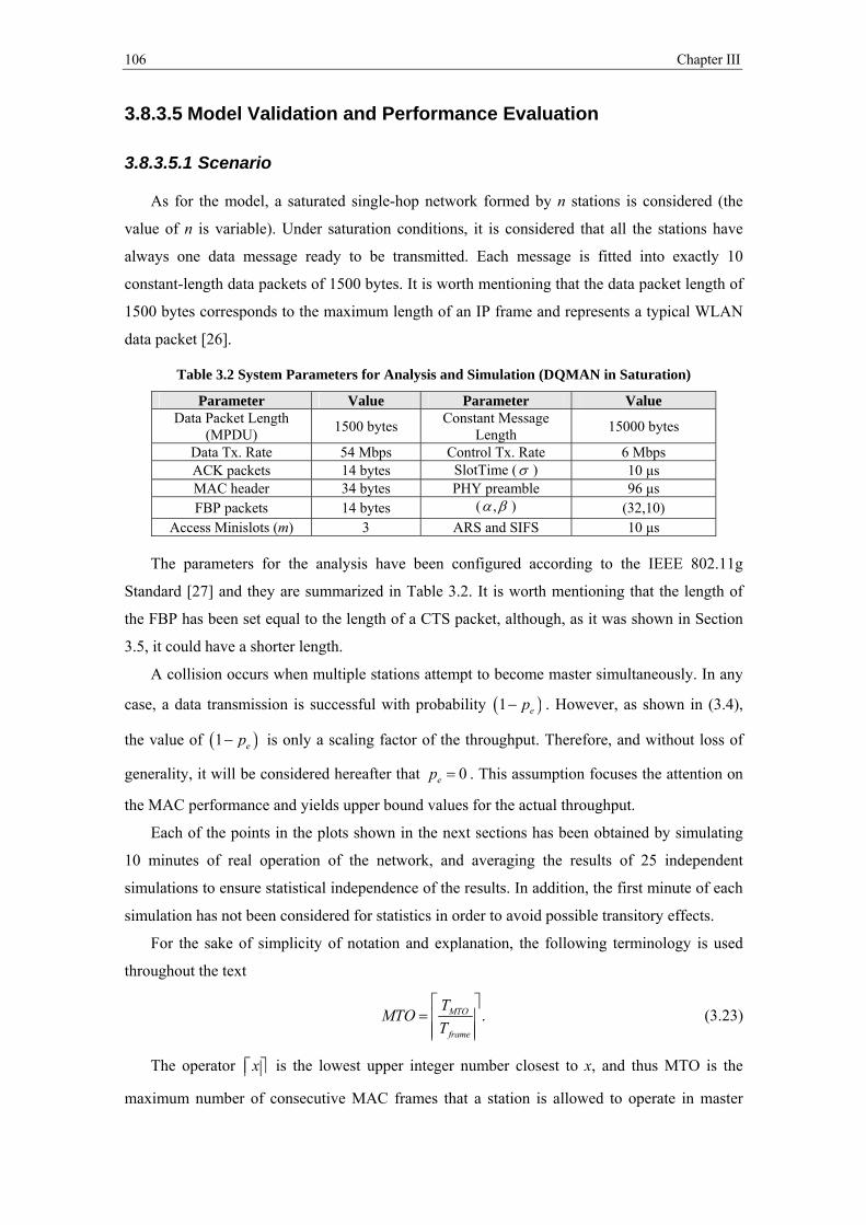
Chapter III
106
3.8.3.5 Model Validation and Performance Evaluation
3.8.3.5.1 Scenario
As for the model, a saturated single-hop network formed by n stations is considered (the
value of n is variable). Under saturation conditions, it is considered that all the stations have
always one data message ready to be transmitted. Each message is fitted into exactly 10
constant-length data packets of 1500 bytes. It is worth mentioning that the data packet length of
1500 bytes corresponds to the maximum length of an IP frame and represents a typical WLAN
data packet [26].
Table 3.2 System Parameters for Analysis and Simulation (DQMAN in Saturation)
Parameter Value Parameter Value Data Packet Length
(MPDU) 1500 bytes
Constant Message Length
15000 bytes
Data Tx. Rate 54 Mbps Control Tx. Rate 6 Mbps ACK packets 14 bytes SlotTime ( ) 10 μs MAC header 34 bytes PHY preamble 96 μs FBP packets 14 bytes ( , ) (32,10)
Access Minislots (m) 3 ARS and SIFS 10 μs
The parameters for the analysis have been configured according to the IEEE 802.11g
Standard [27] and they are summarized in Table 3.2. It is worth mentioning that the length of
the FBP has been set equal to the length of a CTS packet, although, as it was shown in Section
3.5, it could have a shorter length.
A collision occurs when multiple stations attempt to become master simultaneously. In any
case, a data transmission is successful with probability 1 ep . However, as shown in (3.4),
the value of 1 ep is only a scaling factor of the throughput. Therefore, and without loss of
generality, it will be considered hereafter that 0ep . This assumption focuses the attention on
the MAC performance and yields upper bound values for the actual throughput.
Each of the points in the plots shown in the next sections has been obtained by simulating
10 minutes of real operation of the network, and averaging the results of 25 independent
simulations to ensure statistical independence of the results. In addition, the first minute of each
simulation has not been considered for statistics in order to avoid possible transitory effects.
For the sake of simplicity of notation and explanation, the following terminology is used
throughout the text
.MTO
frame
TMTO
T
(3.23)
The operator x is the lowest upper integer number closest to x, and thus MTO is the
maximum number of consecutive MAC frames that a station is allowed to operate in master
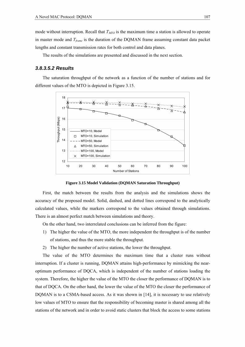
A Novel MAC Protocol: DQMAN
107
mode without interruption. Recall that TMTO is the maximum time a station is allowed to operate
in master mode and Tframe is the duration of the DQMAN frame assuming constant data packet
lengths and constant transmission rates for both control and data planes.
The results of the simulations are presented and discussed in the next section.
3.8.3.5.2 Results
The saturation throughput of the network as a function of the number of stations and for
different values of the MTO is depicted in Figure 3.15.
12
13
14
15
16
17
18
10 20 30 40 50 60 70 80 90 100
Number of Stations
Th
rou
gh
pu
t (M
bp
s)
MTO=10, Model
MTO=10, Simulation
MTO=50, Model
MTO=50, Simulation
MTO=100, Model
MTO=100, Simulation
Figure 3.15 Model Validation (DQMAN Saturation Throughput)
First, the match between the results from the analysis and the simulations shows the
accuracy of the proposed model. Solid, dashed, and dotted lines correspond to the analytically
calculated values, while the markers correspond to the values obtained through simulations.
There is an almost perfect match between simulations and theory.
On the other hand, two interrelated conclusions can be inferred from the figure:
1) The higher the value of the MTO, the more independent the throughput is of the number
of stations, and thus the more stable the throughput.
2) The higher the number of active stations, the lower the throughput.
The value of the MTO determines the maximum time that a cluster runs without
interruption. If a cluster is running, DQMAN attains high-performance by mimicking the near-
optimum performance of DQCA, which is independent of the number of stations loading the
system. Therefore, the higher the value of the MTO the closer the performance of DQMAN is to
that of DQCA. On the other hand, the lower the value of the MTO the closer the performance of
DQMAN is to a CSMA-based access. As it was shown in [14], it is necessary to use relatively
low values of MTO to ensure that the responsibility of becoming master is shared among all the
stations of the network and in order to avoid static clusters that block the access to some stations
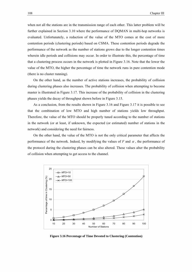
Chapter III
108
when not all the stations are in the transmission range of each other. This latter problem will be
further explained in Section 3.10 where the performance of DQMAN in multi-hop networks is
evaluated. Unfortunately, a reduction of the value of the MTO comes at the cost of more
contention periods (clustering periods) based on CSMA. These contention periods degrade the
performance of the network as the number of stations grows due to the longer contention times
wherein idle periods and collisions may occur. In order to illustrate this, the percentage of time
that a clustering process occurs in the network is plotted in Figure 3.16. Note that the lower the
value of the MTO, the higher the percentage of time the network runs in pure contention mode
(there is no cluster running).
On the other hand, as the number of active stations increases, the probability of collision
during clustering phases also increases. The probability of collision when attempting to become
master is illustrated in Figure 3.17. This increase of the probability of collision in the clustering
phases yields the decay of throughput shown before in Figure 3.15.
As a conclusion, from the results shown in Figure 3.16 and Figure 3.17 it is possible to see
that the combination of low MTO and high number of stations yields low throughput.
Therefore, the value of the MTO should be properly tuned according to the number of stations
in the network (or at least, if unknown, the expected (or estimated) number of stations in the
network) and considering the need for fairness.
On the other hand, the value of the MTO is not the only critical parameter that affects the
performance of the network. Indeed, by modifying the values of F and , the performance of
the protocol during the clustering phases can be also altered. These values alter the probability
of collision when attempting to get access to the channel.
0
5
10
15
20
25
10 20 30 40 50 60 70 80 90 100Number of Stations
Pe
rce
nta
ge
of t
ime
in C
lust
eri
ng
(%
)
MTO=10
MTO=50
MTO=100
Figure 3.16 Percentage of Time Devoted to Clustering (Contention)
A Novel MAC Protocol: DQMAN
109
0
0.1
0.2
0.3
0.4
0.5
0.6
0.7
0.8
0.9
1
10 20 30 40 50 60 70 80 90 100
Number of stations
Pro
ba
bili
ty o
f Co
llisi
on
Figure 3.17 Probability of Collision for F=10 and =32.
16.5
16.7
16.9
17.1
17.3
17.5
17.7
10 20 30 40 50 60 70 80 90 100Number of Stations
Th
rou
gh
pu
t (M
bp
s)
alpha=32 alpha=64 alpha=128 alpha=256
alpha=512 alpha=1024 alpha=2048
Figure 3.18 DQMAN Saturation Throughput with Different Values of
As it was discussed in Section 3.4.4., the value of F has a significant influence on the
probability that a given station operates in master mode during different consecutive (in time)
cluster phases. However, it is shown that its configuration has a minimum influence on the
overall throughput as long as its value is small compared to that of the MTO, which should be a
typical configuration and can be a useful rule of design.
On the other hand, the value of has a direct impact on the probability of collision when
attempting to become master. In order to assess its impact on the performance of the network,
and without loss of generality, the value of the MTO is fixed to 50 and the value of F to 10. The
saturation throughput of the network as a function of the number of stations and for different
values of is illustrated in Figure 3.18. It can be inferred from this figure that if the value of
is small when compared to the number of active stations, the performance of the network is
Chapter III
110
slightly degraded. For example, when 32 and with 100 stations contending in the network,
the probability of collision is such that the saturation throughput of the network drops
remarkably from 17.5 Mbps for 10 stations to 16.6 Mbps for 100 stations (6%).
Therefore, higher values of may improve the performance of DQMAN but can also lead
to a waste of time in deferral periods if the number of stations in the network is small.
Therefore, the value of should be (dynamically) adjusted to the number of active stations in
the network. In any case, and as it was shown in Figure 3.15, the effects of the configuration of
the network (values of F and ) become less significant as the value of the MTO increases.
This is mainly due to the fact that the performance of the MAC protocol executed within each
cluster is independent of the number of active stations and higher values of MTO lead to longer
periods of clustered operation compared to CSMA-based clustering phases.
3.8.3.6 Comparison with the IEEE 802.11 MAC Protocol
A comparison between the saturation throughput of a DQMAN network and that of a legacy
network just using the MAC of the IEEE 802.11 Standard is presented in this section. The
results presented in this section have been obtained through computer simulation with
MACSWIN.
3.8.3.6.1 Scenario
The same scenario as the one described in the previous section is considered for this
evaluation. In this case, three different ad hoc networks are considered:
1) A network where the stations execute DQMAN.
2) A network where the stations execute the basic access mode of IEEE 802.11.
3) A network where the stations execute the collision avoidance access mode of IEEE
802.11 with RTS/CTS handshake between source and destination.
As in the previous section, the value of the MTO in the DQMAN network corresponds to
the maximum number of consecutive MAC frames that a station is allowed to operate in master
mode without interruption and it has been fixed to 50 for this evaluation (note that this yields
low performance of DQMAN). The rest of the parameters, for both the DQMAN and the legacy
standard, are summarized in Table 3.3.
As in the previous section, each of the points in the plots shown in the next sections have
been obtained by simulating 10 minutes of real operation of the network, and averaging the
results of 25 independent simulations to ensure the statistical independence of the results. In
addition, the first minute of each simulation has not been considered for statistics in order to
avoid possible transitory effects.
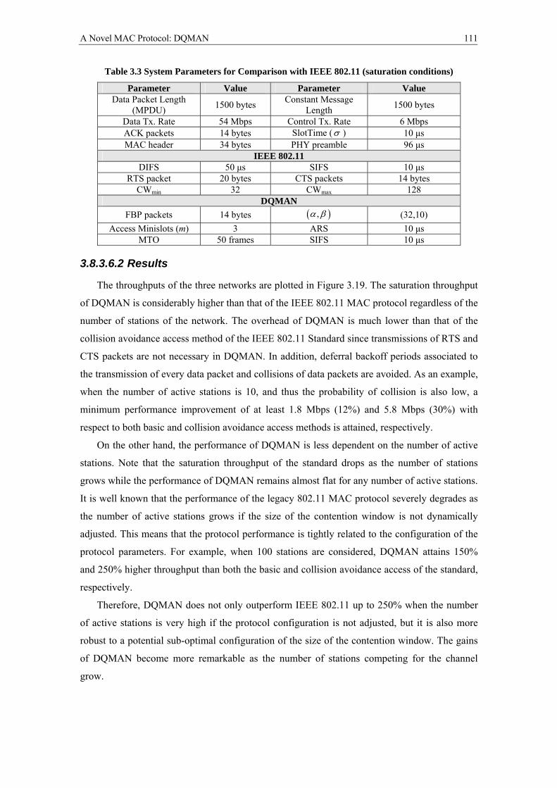
A Novel MAC Protocol: DQMAN
111
Table 3.3 System Parameters for Comparison with IEEE 802.11 (saturation conditions)
Parameter Value Parameter Value Data Packet Length
(MPDU) 1500 bytes
Constant Message Length
1500 bytes
Data Tx. Rate 54 Mbps Control Tx. Rate 6 Mbps ACK packets 14 bytes SlotTime ( ) 10 μs MAC header 34 bytes PHY preamble 96 μs
IEEE 802.11 DIFS 50 μs SIFS 10 μs
RTS packet 20 bytes CTS packets 14 bytes CWmin 32 CWmax 128
DQMAN
FBP packets 14 bytes , (32,10)
Access Minislots (m) 3 ARS 10 μs MTO 50 frames SIFS 10 μs
3.8.3.6.2 Results
The throughputs of the three networks are plotted in Figure 3.19. The saturation throughput
of DQMAN is considerably higher than that of the IEEE 802.11 MAC protocol regardless of the
number of stations of the network. The overhead of DQMAN is much lower than that of the
collision avoidance access method of the IEEE 802.11 Standard since transmissions of RTS and
CTS packets are not necessary in DQMAN. In addition, deferral backoff periods associated to
the transmission of every data packet and collisions of data packets are avoided. As an example,
when the number of active stations is 10, and thus the probability of collision is also low, a
minimum performance improvement of at least 1.8 Mbps (12%) and 5.8 Mbps (30%) with
respect to both basic and collision avoidance access methods is attained, respectively.
On the other hand, the performance of DQMAN is less dependent on the number of active
stations. Note that the saturation throughput of the standard drops as the number of stations
grows while the performance of DQMAN remains almost flat for any number of active stations.
It is well known that the performance of the legacy 802.11 MAC protocol severely degrades as
the number of active stations grows if the size of the contention window is not dynamically
adjusted. This means that the protocol performance is tightly related to the configuration of the
protocol parameters. For example, when 100 stations are considered, DQMAN attains 150%
and 250% higher throughput than both the basic and collision avoidance access of the standard,
respectively.
Therefore, DQMAN does not only outperform IEEE 802.11 up to 250% when the number
of active stations is very high if the protocol configuration is not adjusted, but it is also more
robust to a potential sub-optimal configuration of the size of the contention window. The gains
of DQMAN become more remarkable as the number of stations competing for the channel
grow.
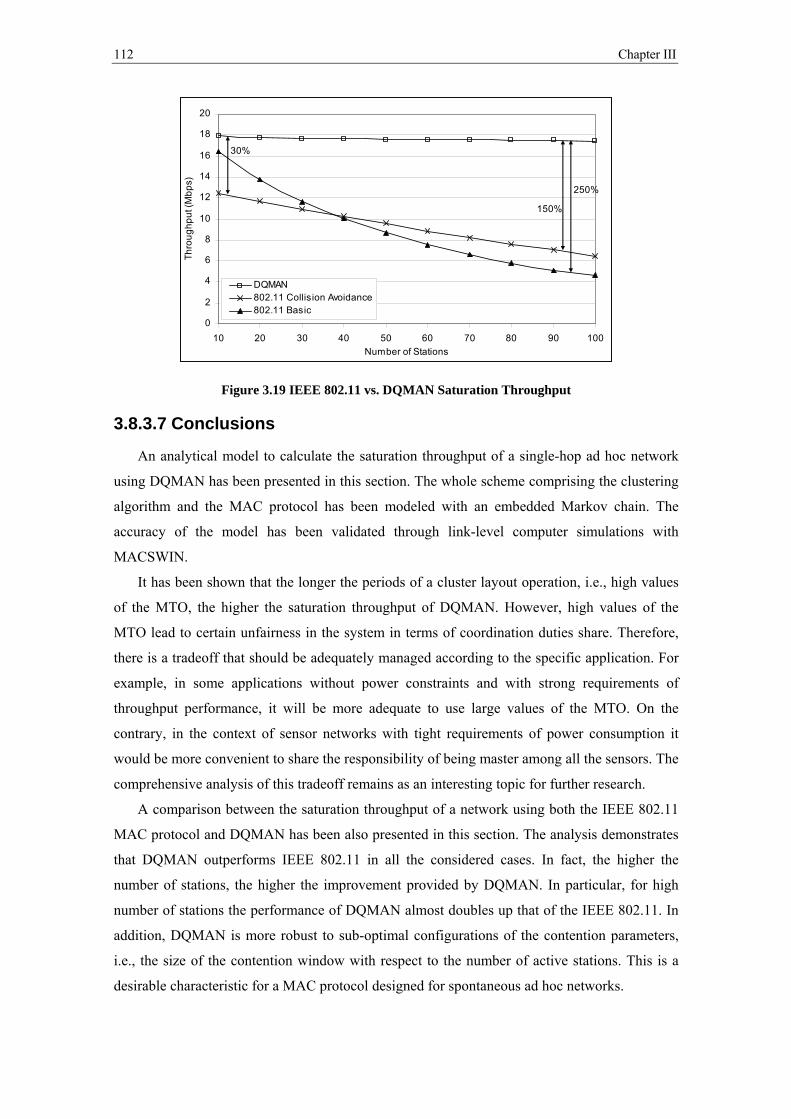
Chapter III
112
0
2
4
6
8
10
12
14
16
18
20
10 20 30 40 50 60 70 80 90 100
Number of Stations
Th
rou
gh
pu
t (M
bp
s)
DQMAN802.11 Collision Avoidance802.11 Basic
30%
150%
250%
Figure 3.19 IEEE 802.11 vs. DQMAN Saturation Throughput
3.8.3.7 Conclusions
An analytical model to calculate the saturation throughput of a single-hop ad hoc network
using DQMAN has been presented in this section. The whole scheme comprising the clustering
algorithm and the MAC protocol has been modeled with an embedded Markov chain. The
accuracy of the model has been validated through link-level computer simulations with
MACSWIN.
It has been shown that the longer the periods of a cluster layout operation, i.e., high values
of the MTO, the higher the saturation throughput of DQMAN. However, high values of the
MTO lead to certain unfairness in the system in terms of coordination duties share. Therefore,
there is a tradeoff that should be adequately managed according to the specific application. For
example, in some applications without power constraints and with strong requirements of
throughput performance, it will be more adequate to use large values of the MTO. On the
contrary, in the context of sensor networks with tight requirements of power consumption it
would be more convenient to share the responsibility of being master among all the sensors. The
comprehensive analysis of this tradeoff remains as an interesting topic for further research.
A comparison between the saturation throughput of a network using both the IEEE 802.11
MAC protocol and DQMAN has been also presented in this section. The analysis demonstrates
that DQMAN outperforms IEEE 802.11 in all the considered cases. In fact, the higher the
number of stations, the higher the improvement provided by DQMAN. In particular, for high
number of stations the performance of DQMAN almost doubles up that of the IEEE 802.11. In
addition, DQMAN is more robust to sub-optimal configurations of the contention parameters,
i.e., the size of the contention window with respect to the number of active stations. This is a
desirable characteristic for a MAC protocol designed for spontaneous ad hoc networks.
A Novel MAC Protocol: DQMAN
113
Finally, it is worth mentioning that the model herein presented could be easily adapted to
any other MAC protocol based on the DQMAN clustering.
In the next section, the model is extended to analyze the performance of DQMAN under
non-saturated conditions. The specific approach is to consider Poisson distributed arrivals rather
than considering that all the stations have always at least one packet ready to be transmitted.
3.8.4 Analysis in Non-Saturation Conditions
The previous analysis is extended in this section to general non-saturation traffic conditions,
i.e., an arbitrary traffic input rate, which constitutes a more challenging problem. In fact, there
are few analytical models in the literature regarding the non-saturation performance of MAC
protocols, as it was discussed in Section 1.2.2 of Chapter I.
Without loss of generality, now it is considered that all the stations generate Poisson
distributed data messages (MSDUs or MMDUs) whose length is an exponential random
variable with average 1/ ·L bits. All the n stations generate the same average traffic load,
and the aggregated message arrival rate is (messages/second). Once a message is generated,
its destination is chosen at random among the n–1 neighbors, all of them with equal probability.
These messages are fragmented into fixed-length data packets of L bits and buffered into
infinite-size buffers before being transmitted through the radio interface. Exactly one data
packet of length L is transmitted within the data part of each single MAC frame (see Figure 3.5
in the description of the protocol). Note that with this definition 1/ μ corresponds to the average
number of fragments of a message.
3.8.4.1 Overview
Recall Section 3.8.2.2 where the superslot structure was introduced as an abstraction tool to
model the network. Superslots allow defining the network (as a whole) as a semi-markovian
process with three different states. The associated embedded Markov chain is again illustrated
in Figure 3.20. Changes in the state of the network occur at the end of each superslot.
Having this model in mind, the proposed analytical model to evaluate the performance of
DQMAN consists of two parts:
1) Transitions between states in the network are modeled with an embedded Markov chain
that extends the chain in Figure 3.20 to consider the operation details of DQMAN.
2) Once a cluster is running, the performance of the network can be modeled with classical
queueing theory, modeling the operation of the modified DQCA protocol used within
DQMAN.
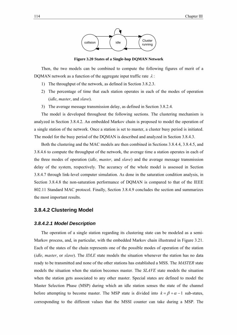
Chapter III
114
idlecollisionCluster running
Figure 3.20 States of a Single-hop DQMAN Network
Then, the two models can be combined to compute the following figures of merit of a
DQMAN network as a function of the aggregate input traffic rate :
1) The throughput of the network, as defined in Section 3.8.2.3.
2) The percentage of time that each station operates in each of the modes of operation
(idle, master, and slave).
3) The average message transmission delay, as defined in Section 3.8.2.4.
The model is developed throughout the following sections. The clustering mechanism is
analyzed in Section 3.8.4.2. An embedded Markov chain is proposed to model the operation of
a single station of the network. Once a station is set to master, a cluster busy period is initiated.
The model for the busy period of the DQMAN is described and analyzed in Section 3.8.4.3.
Both the clustering and the MAC models are then combined in Sections 3.8.4.4, 3.8.4.5, and
3.8.4.6 to compute the throughput of the network, the average time a station operates in each of
the three modes of operation (idle, master, and slave) and the average message transmission
delay of the system, respectively. The accuracy of the whole model is assessed in Section
3.8.4.7 through link-level computer simulation. As done in the saturation condition analysis, in
Section 3.8.4.8 the non-saturation performance of DQMAN is compared to that of the IEEE
802.11 Standard MAC protocol. Finally, Section 3.8.4.9 concludes the section and summarizes
the most important results.
3.8.4.2 Clustering Model
3.8.4.2.1 Model Description
The operation of a single station regarding its clustering state can be modeled as a semi-
Markov process, and, in particular, with the embedded Markov chain illustrated in Figure 3.21.
Each of the states of the chain represents one of the possible modes of operation of the station
(idle, master, or slave). The IDLE state models the situation whenever the station has no data
ready to be transmitted and none of the other stations has established a MSS. The MASTER state
models the situation when the station becomes master. The SLAVE state models the situation
when the station gets associated to any other master. Special states are defined to model the
Master Selection Phase (MSP) during which an idle station senses the state of the channel
before attempting to become master. The MSP state is divided into 1k sub-states,
corresponding to the different values that the MSSI counter can take during a MSP. The
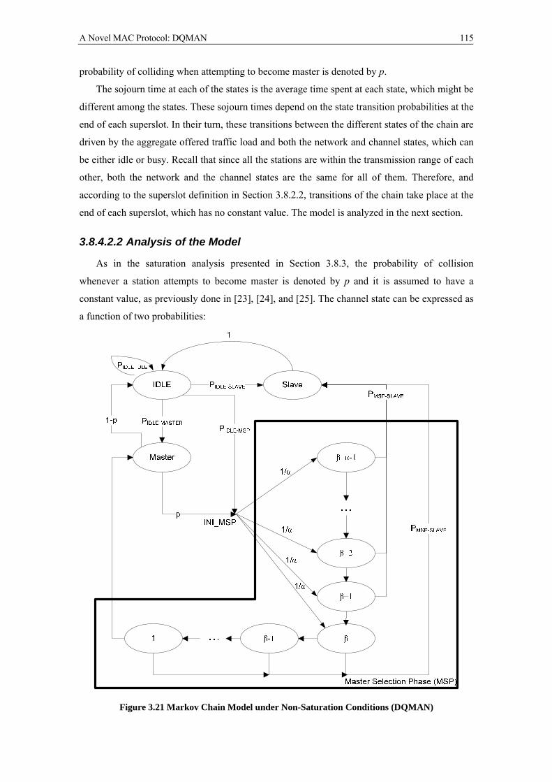
A Novel MAC Protocol: DQMAN
115
probability of colliding when attempting to become master is denoted by p.
The sojourn time at each of the states is the average time spent at each state, which might be
different among the states. These sojourn times depend on the state transition probabilities at the
end of each superslot. In their turn, these transitions between the different states of the chain are
driven by the aggregate offered traffic load and both the network and channel states, which can
be either idle or busy. Recall that since all the stations are within the transmission range of each
other, both the network and the channel states are the same for all of them. Therefore, and
according to the superslot definition in Section 3.8.2.2, transitions of the chain take place at the
end of each superslot, which has no constant value. The model is analyzed in the next section.
3.8.4.2.2 Analysis of the Model
As in the saturation analysis presented in Section 3.8.3, the probability of collision
whenever a station attempts to become master is denoted by p and it is assumed to have a
constant value, as previously done in [23], [24], and [25]. The channel state can be expressed as
a function of two probabilities:
Figure 3.21 Markov Chain Model under Non-Saturation Conditions (DQMAN)
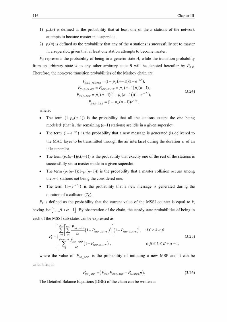
Chapter III
116
1) ptr(n) is defined as the probability that at least one of the n stations of the network
attempts to become master in a superslot.
2) ps(n) is defined as the probability that any of the n stations is successfully set to master
in a superslot, given that at least one station attempts to become master.
PA represents the probability of being in a generic state A, while the transition probability
from an arbitrary state A to any other arbitrary state B will be denoted hereafter by PA-B.
Therefore, the non-zero transition probabilities of the Markov chain are
(1 ( 1))(1 ),
( 1) ( 1),
( 1) 1 ( 1) (1 ),
(1 ( 1)) ,
IDLE MASTER tr
IDLE SLAVE MSP SLAVE tr s
TcIDLE MSP tr s
IDLE IDLE tr
P p n e
P P p n p n
P p n p n e
P p n e
(3.24)
where:
The term (1–ptr(n–1)) is the probability that all the stations except the one being
modeled (that is, the remaining (n–1) stations) are idle in a given superslot.
The term (1 )e is the probability that a new message is generated (is delivered to
the MAC layer to be transmitted through the air interface) during the duration of an
idle superslot.
The term (ptr(n–1)ps(n–1)) is the probability that exactly one of the rest of the stations is
successfully set to master mode in a given superslot.
The term (ptr(n–1)(1–ps(n–1))) is the probability that a master collision occurs among
the n–1 stations not being the considered one.
The term (1 )CTe is the probability that a new message is generated during the
duration of a collision (TC).
Pk is defined as the probability that the current value of the MSSI counter is equal to k,
having 1,.., 1k . By observation of the chain, the steady state probabilities of being in
each of the MSSI sub-states can be expressed as
1_
i=1 j=0
1_
i=0
1 1 , if 0
1 , if 1,
kj iINI MSP
MSP SLAVE MSP SLAVE
kk
iINI MSPMSP SLAVE
PP P k
PP
P k
(3.25)
where the value of _INI MSPP is the probability of initiating a new MSP and it can be
calculated as
_ .INI MSP IDLE IDLE MSP MASTERP P P P p (3.26)
The Detailed Balance Equations (DBE) of the chain can be written as
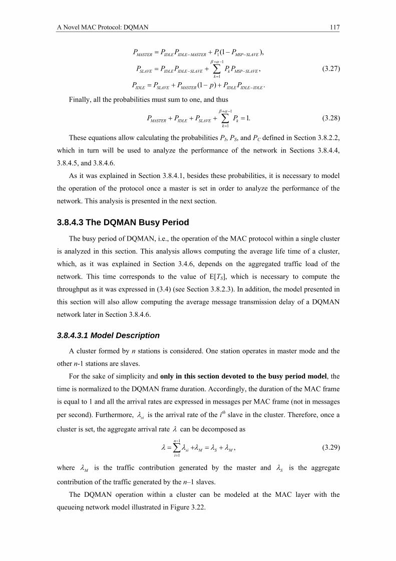
A Novel MAC Protocol: DQMAN
117
1
1
1
(1 ),
,
(1 ) .
MASTER IDLE IDLE MASTER MSP SLAVE
SLAVE IDLE IDLE SLAVE k MSP SLAVEk
IDLE SLAVE MASTER IDLE IDLE IDLE
P P P P P
P P P P P
P P P p P P
(3.27)
Finally, all the probabilities must sum to one, and thus
1
1
1.MASTER IDLE SLAVE kk
P P P P
(3.28)
These equations allow calculating the probabilities PI, PS, and PC defined in Section 3.8.2.2,
which in turn will be used to analyze the performance of the network in Sections 3.8.4.4,
3.8.4.5, and 3.8.4.6.
As it was explained in Section 3.8.4.1, besides these probabilities, it is necessary to model
the operation of the protocol once a master is set in order to analyze the performance of the
network. This analysis is presented in the next section.
3.8.4.3 The DQMAN Busy Period
The busy period of DQMAN, i.e., the operation of the MAC protocol within a single cluster
is analyzed in this section. This analysis allows computing the average life time of a cluster,
which, as it was explained in Section 3.4.6, depends on the aggregated traffic load of the
network. This time corresponds to the value of E[TS], which is necessary to compute the
throughput as it was expressed in (3.4) (see Section 3.8.2.3). In addition, the model presented in
this section will also allow computing the average message transmission delay of a DQMAN
network later in Section 3.8.4.6.
3.8.4.3.1 Model Description
A cluster formed by n stations is considered. One station operates in master mode and the
other n-1 stations are slaves.
For the sake of simplicity and only in this section devoted to the busy period model, the
time is normalized to the DQMAN frame duration. Accordingly, the duration of the MAC frame
is equal to 1 and all the arrival rates are expressed in messages per MAC frame (not in messages
per second). Furthermore, si is the arrival rate of the ith slave in the cluster. Therefore, once a
cluster is set, the aggregate arrival rate can be decomposed as
1
1
,n
si M S Mi
(3.29)
where M is the traffic contribution generated by the master and S is the aggregate
contribution of the traffic generated by the n–1 slaves.
The DQMAN operation within a cluster can be modeled at the MAC layer with the
queueing network model illustrated in Figure 3.22.
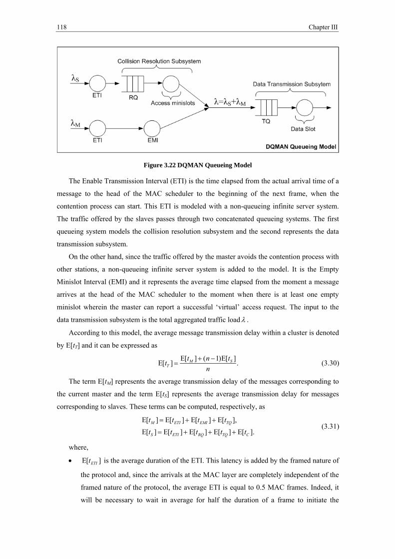
Chapter III
118
Figure 3.22 DQMAN Queueing Model
The Enable Transmission Interval (ETI) is the time elapsed from the actual arrival time of a
message to the head of the MAC scheduler to the beginning of the next frame, when the
contention process can start. This ETI is modeled with a non-queueing infinite server system.
The traffic offered by the slaves passes through two concatenated queueing systems. The first
queueing system models the collision resolution subsystem and the second represents the data
transmission subsystem.
On the other hand, since the traffic offered by the master avoids the contention process with
other stations, a non-queueing infinite server system is added to the model. It is the Empty
Minislot Interval (EMI) and it represents the average time elapsed from the moment a message
arrives at the head of the MAC scheduler to the moment when there is at least one empty
minislot wherein the master can report a successful ‘virtual’ access request. The input to the
data transmission subsystem is the total aggregated traffic load .
According to this model, the average message transmission delay within a cluster is denoted
by E[tT] and it can be expressed as
E[ ] ( 1)E[ ]
E[ ] .M ST
t n tt
n
(3.30)
The term E[tM] represents the average transmission delay of the messages corresponding to
the current master and the term E[tS] represents the average transmission delay for messages
corresponding to slaves. These terms can be computed, respectively, as
E[ ] E[ ] E[ ] E[ ],
E[ ] E[ ] E[ ] E[ ] E[ ].
M ETI EMI TQ
S ETI RQ TQ C
t t t t
t t t t t
(3.31)
where,
E[ ]ETIt is the average duration of the ETI. This latency is added by the framed nature of
the protocol and, since the arrivals at the MAC layer are completely independent of the
framed nature of the protocol, the average ETI is equal to 0.5 MAC frames. Indeed, it
will be necessary to wait in average for half the duration of a frame to initiate the
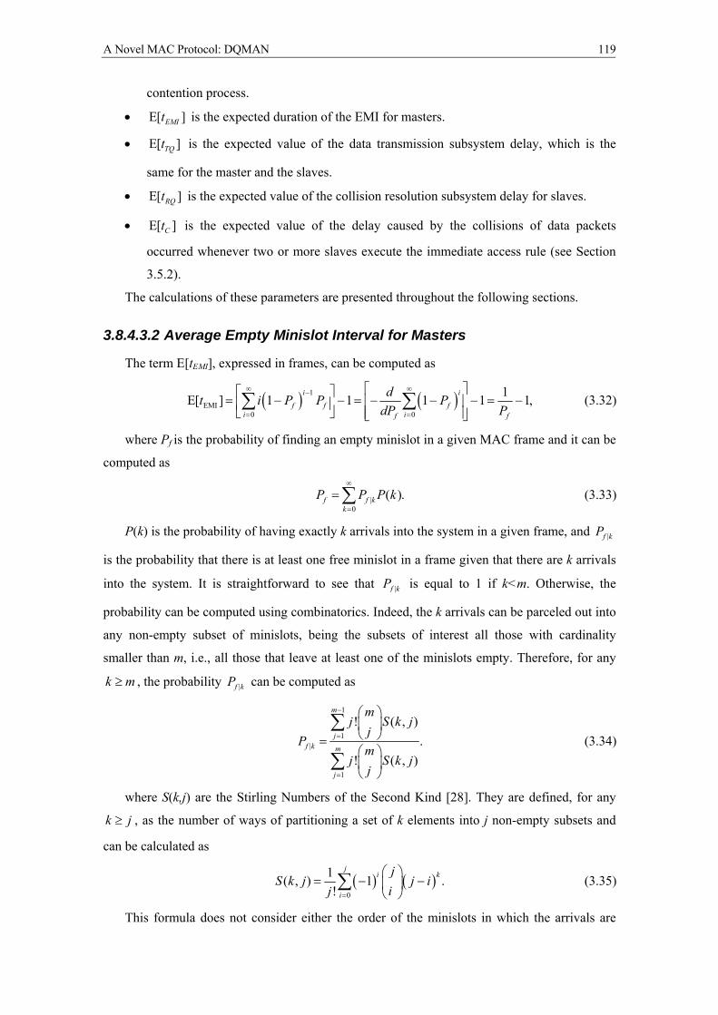
A Novel MAC Protocol: DQMAN
119
contention process.
E[ ]EMIt is the expected duration of the EMI for masters.
E[ ]TQt is the expected value of the data transmission subsystem delay, which is the
same for the master and the slaves.
E[ ]RQt is the expected value of the collision resolution subsystem delay for slaves.
E[ ]Ct is the expected value of the delay caused by the collisions of data packets
occurred whenever two or more slaves execute the immediate access rule (see Section
3.5.2).
The calculations of these parameters are presented throughout the following sections.
3.8.4.3.2 Average Empty Minislot Interval for Masters
The term E[tEMI], expressed in frames, can be computed as
1
EMI0 0
1E[ ] 1 1 1 1 1,
i i
f f fi if f
dt i P P P
dP P
(3.32)
where Pf is the probability of finding an empty minislot in a given MAC frame and it can be
computed as
|0
( ).f f kk
P P P k
(3.33)
P(k) is the probability of having exactly k arrivals into the system in a given frame, and |f kP
is the probability that there is at least one free minislot in a frame given that there are k arrivals
into the system. It is straightforward to see that |f kP is equal to 1 if k<m. Otherwise, the
probability can be computed using combinatorics. Indeed, the k arrivals can be parceled out into
any non-empty subset of minislots, being the subsets of interest all those with cardinality
smaller than m, i.e., all those that leave at least one of the minislots empty. Therefore, for any
k m , the probability |f kP can be computed as
1
1|
1
! ( , )
.
! ( , )
m
jf k m
j
mj S k j
jP
mj S k j
j
(3.34)
where S(k,j) are the Stirling Numbers of the Second Kind [28]. They are defined, for any
k j , as the number of ways of partitioning a set of k elements into j non-empty subsets and
can be calculated as
0
1( , ) 1 .
!
ji k
i
jS k j j i
ij
(3.35)
This formula does not consider either the order of the minislots in which the arrivals are
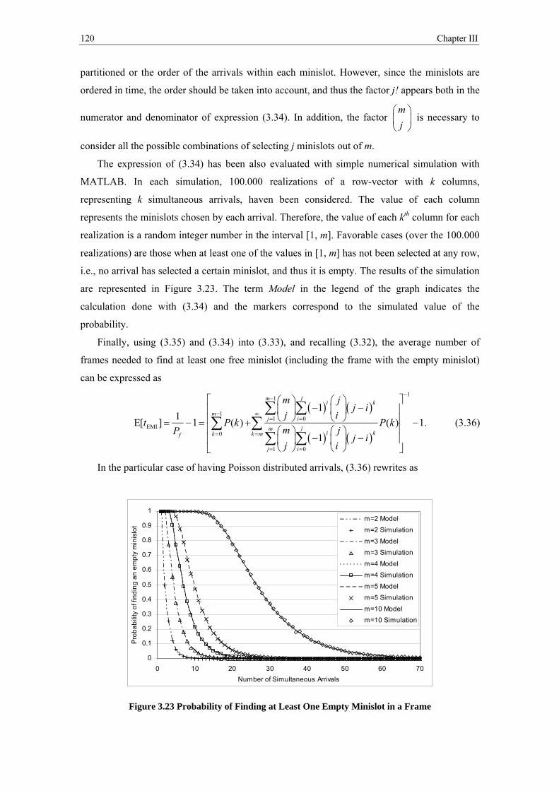
Chapter III
120
partitioned or the order of the arrivals within each minislot. However, since the minislots are
ordered in time, the order should be taken into account, and thus the factor j! appears both in the
numerator and denominator of expression (3.34). In addition, the factor m
j
is necessary to
consider all the possible combinations of selecting j minislots out of m.
The expression of (3.34) has been also evaluated with simple numerical simulation with
MATLAB. In each simulation, 100.000 realizations of a row-vector with k columns,
representing k simultaneous arrivals, haven been considered. The value of each column
represents the minislots chosen by each arrival. Therefore, the value of each kth column for each
realization is a random integer number in the interval [1, m]. Favorable cases (over the 100.000
realizations) are those when at least one of the values in [1, m] has not been selected at any row,
i.e., no arrival has selected a certain minislot, and thus it is empty. The results of the simulation
are represented in Figure 3.23. The term Model in the legend of the graph indicates the
calculation done with (3.34) and the markers correspond to the simulated value of the
probability.
Finally, using (3.35) and (3.34) into (3.33), and recalling (3.32), the average number of
frames needed to find at least one free minislot (including the frame with the empty minislot)
can be expressed as
11
11 0
EMI0
1 0
11
E[ ] 1 ( ) ( ) 1.
1
jmi k
mj i
jmi kk k mf
j i
m jj i
j it P k P k
m jPj i
j i
(3.36)
In the particular case of having Poisson distributed arrivals, (3.36) rewrites as
0
0.1
0.2
0.3
0.4
0.5
0.6
0.7
0.8
0.9
1
0 10 20 30 40 50 60 70
Number of Simultaneous Arrivals
Pro
ba
bili
ty o
f fin
din
g a
n e
mp
ty m
inis
lot
m=2 Model
m=2 Simulation
m=3 Model
m=3 Simulation
m=4 Model
m=4 Simulation
m=5 Model
m=5 Simulation
m=10 Model
m=10 Simulation
Figure 3.23 Probability of Finding at Least One Empty Minislot in a Frame
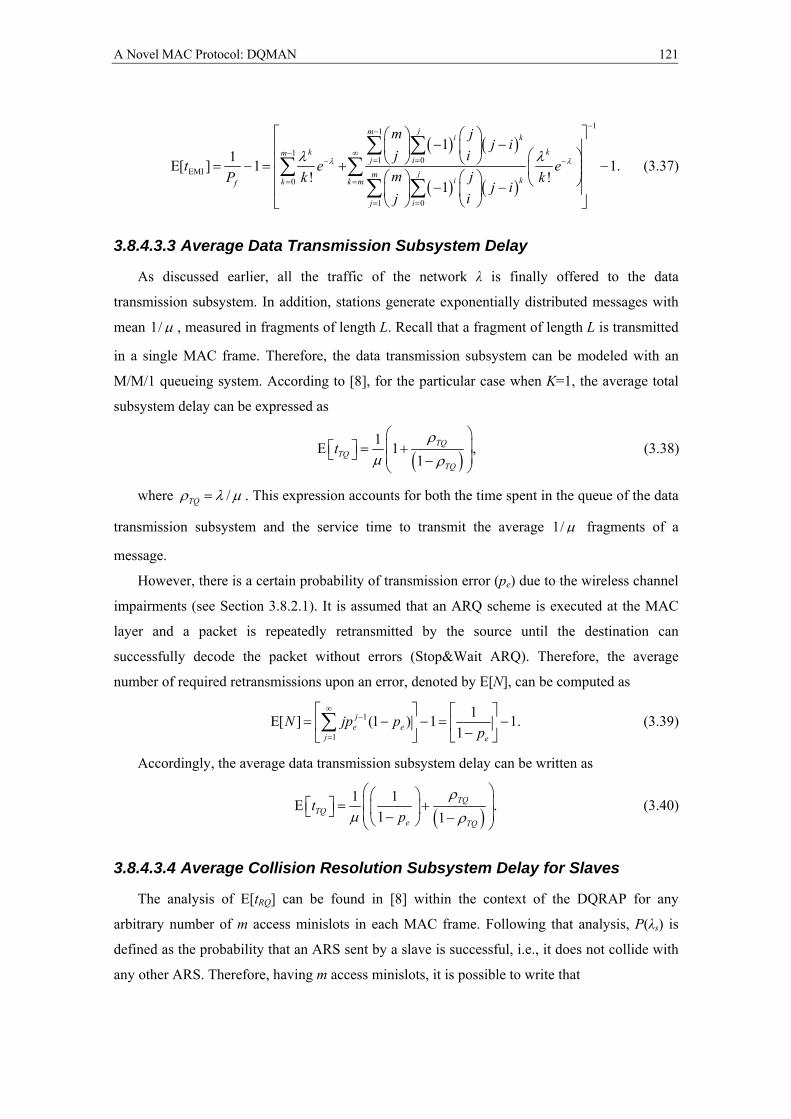
A Novel MAC Protocol: DQMAN
121
11
11 0
EMI0
1 0
11
E[ ] 1 1.! !
1
jmi k
k kmj i
jmi kk k mf
j i
m jj i
j it e e
m jP k kj i
j i
(3.37)
3.8.4.3.3 Average Data Transmission Subsystem Delay
As discussed earlier, all the traffic of the network λ is finally offered to the data
transmission subsystem. In addition, stations generate exponentially distributed messages with
mean 1/ , measured in fragments of length L. Recall that a fragment of length L is transmitted
in a single MAC frame. Therefore, the data transmission subsystem can be modeled with an
M/M/1 queueing system. According to [8], for the particular case when K=1, the average total
subsystem delay can be expressed as
1E 1 ,
1TQ
TQ
TQ
t
(3.38)
where /TQ . This expression accounts for both the time spent in the queue of the data
transmission subsystem and the service time to transmit the average 1/ fragments of a
message.
However, there is a certain probability of transmission error (pe) due to the wireless channel
impairments (see Section 3.8.2.1). It is assumed that an ARQ scheme is executed at the MAC
layer and a packet is repeatedly retransmitted by the source until the destination can
successfully decode the packet without errors (Stop&Wait ARQ). Therefore, the average
number of required retransmissions upon an error, denoted by E[N], can be computed as
1
1
1E[ ] (1 ) 1 1.
1j
e ej e
N jp pp
(3.39)
Accordingly, the average data transmission subsystem delay can be written as
1 1E .
1 1TQ
TQe TQ
tp
(3.40)
3.8.4.3.4 Average Collision Resolution Subsystem Delay for Slaves
The analysis of E[tRQ] can be found in [8] within the context of the DQRAP for any
arbitrary number of m access minislots in each MAC frame. Following that analysis, P(λs) is
defined as the probability that an ARS sent by a slave is successful, i.e., it does not collide with
any other ARS. Therefore, having m access minislots, it is possible to write that
Chapter III
122
0
( ) ( _ | ) ( ).sk
P P free minislot k P k
(3.41)
( _ | )P free minislot k is the probability of choosing a free minislot when k ARS have been
sent in a given frame and ( )P k is the probability that exactly k ARS have been sent in a same
frame. Therefore, it is possible to write that
1 1
11
1
1 1 1( ) (0) ( ) 1 1
!
111 .
!
s s
ss
s s
k kkks
sk k
k
s m m
k
P P P k m e em m k m
me e e e
k m
(3.42)
Note that λs/m is the average traffic offered by the slaves to each of the m access minislots
and that all the messages in the collision resolution subsystem have the same probability P(λs)
of having a successful ARS transmission. Therefore, the service time of the collision resolution
subsystem will be a discrete geometric random variable, with the following Probability
Distribution Function (PDF),
( ) 1 1 ( ) ,t
RQ sF t P (3.43)
where [t] is the closest integer to t.
Using the exact Probability Density Function (pdf), the collision resolution subsystem
would be represented by an M/G/1 queueing model. As demonstrated in [29], this kind of
systems is not tractable analytically. However, since the values of the geometric distribution are
samples of the exponential distribution, it is possible to approximate the geometric distribution
with an exponential distribution in continuous time t. Therefore, the expression of the pdf of the
collision resolution subsystem service is given by
( ) 1
( ) 1 ( ) ln ,1 ( )
tRQRQ s
s
F tf t P
t P
(3.44)
which is equivalent to a Poisson variable with mean
1
1 1ln .
1 ( )RQ sP
(3.45)
Consequently, the collision resolution subsystem can be modeled as an M/M/1 queueing
system. In order to analyze the total service time, the utilization factor RQ is defined as
1.sRQ
RQ
(3.46)
1/ RQ is the average server service time as defined in (3.45). Therefore, the probability of
having j units in the collision resolution subsystem is determined by
0 ,jj RQp p (3.47)
A Novel MAC Protocol: DQMAN
123
where,
1
0 1 .1
RQ
RQ
p
(3.48)
The total average time spent in the collision resolution subsystem can be calculated from
these expressions as the average service time plus the average queueing time, resulting in
1E[ ] ,
1RQ
RQRQ RQ RQ
Pt
(3.49)
where PRQ is the delay probability, i.e., the probability that a message has to wait in the queue
when it arrives at the system. This is equivalent to the probability that the system contains at
least one message either being served or queueing to be served, and it is expressed as
00
1 1
1.
1 11
RQ
j RQRQRQ j RQ
RQj j RQ
RQ
pP p p
(3.50)
Finally, the expectation of the total delay of the collision resolution subsystem can be
written as
/
1E 1 .
1 1ln1 s
RQRQ
RQm
t
e
(3.51)
3.8.4.3.5 Average Data Collision Delay
Only the traffic contribution from slaves is considered for this calculation as the master will
never generate a collision. Then, the considered input rate is now s and according to the
analysis in [8] for the case when K=1, the average waiting time will be less than one and equal
to the probability of data collision, i.e.,
0 02
_ 1
E[ ] 1!
11 1 1 1 1 .
11
s
s s
s s
ks
C sk
slave arrivals
s RQ sRQ
RQ
et p p e e
k
e e
(3.52)
At this point in the analysis, all the delay contributions expressed in (3.31) to compute the
average message transmission delay during a DQMAN busy period have been derived. The
evaluation of this expression considering different network configurations has been
intentionally left for Section 3.8.4.7. Before that, the non-saturation throughput of DQMAN is
analyzed in the next section.
Chapter III
124
3.8.4.4 Throughput Analysis
An embedded Markov chain has been presented and analyzed in Section 3.8.4.2 to model
the clustering algorithm of DQMAN. Then, in Section 3.8.4.3, the performance of the MAC
protocol once a cluster is set has been modeled with a queueing network model. The aim of this
section and the two following sections is to combine both models to compute the throughput,
the average message transmission delay, and the average time spent in each mode of operation,
respectively, within the context of a DQMAN network.
The particular focus in this section is on calculating the non-saturated throughput of
DQMAN as a function of the offered traffic load. The throughput was defined in (3.4) (see
Section 3.8.2.3). In order to compute this expression, it is necessary to obtain the values of PS,
PI, PC, and E[TS]. Recall that the values of TI and TC are deterministic values as defined in
Section 3.8.2.2.
The value of E[TS] corresponds to the average duration of a DQMAN busy period, i.e., the
average time that a station operates in master mode without interruption. Considering the model
presented in Figure 3.22, this calculation is not a trivial task. In order to simplify its calculation,
the following approximation has been adopted: the input data rate of the master also enters the
collision resolution subsystem of the slave stations. Therefore, the complete model illustrated in
Figure 3.22 turns into the simplified model represented in Figure 3.24 that provides a lower
bound of E[TS]. The accuracy of this approximation will be then validated through computer
simulation when the complete model is assessed. It is important to emphasize that this
simplification has only been done for the computation of the average duration of a DQMAN
busy period and not for the rest of the analysis.
According to the definition in Section 2.3.5 of Chapter II, the utilization factor of a tandem
of queues can be computed as
E[ ]
,E[ ] E[ ]
BUSYTANDEM
IDLE BUSY
T
T T
(3.53)
with E[TIDLE] and E[TBUSY] the average duration of the idle and busy periods of the tandem,
respectively. Therefore, it is possible to isolate the average duration of the busy period of a
tandem of queues from (3.53) as
E[ ] E[ ] ,1
TANDEMBUSY IDLE
TANDEM
T T
(3.54)
from which it is straightforward to obtain that the value of E[Ts], measured in MAC frames, can
be calculated as the duration of the initial master sensing interval plus the average busy period
of a tandem of two M/M/1 queueing systems, and thus
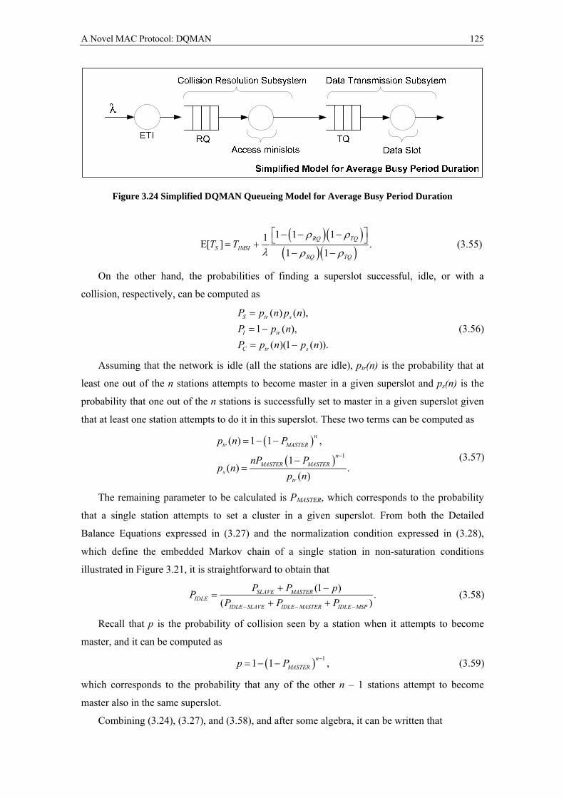
A Novel MAC Protocol: DQMAN
125
Figure 3.24 Simplified DQMAN Queueing Model for Average Busy Period Duration
1 1 11
E[ ] .1 1
RQ TQ
S IMSI
RQ TQ
T T
(3.55)
On the other hand, the probabilities of finding a superslot successful, idle, or with a
collision, respectively, can be computed as
( ) ( ),
1 ( ),
( )(1 ( )).
S tr s
I tr
C tr s
P p n p n
P p n
P p n p n
(3.56)
Assuming that the network is idle (all the stations are idle), ptr(n) is the probability that at
least one out of the n stations attempts to become master in a given superslot and ps(n) is the
probability that one out of the n stations is successfully set to master in a given superslot given
that at least one station attempts to do it in this superslot. These two terms can be computed as
1
( ) 1 1 ,
1( ) .
( )
n
tr MASTER
n
MASTER MASTERs
tr
p n P
nP Pp n
p n
(3.57)
The remaining parameter to be calculated is PMASTER, which corresponds to the probability
that a single station attempts to set a cluster in a given superslot. From both the Detailed
Balance Equations expressed in (3.27) and the normalization condition expressed in (3.28),
which define the embedded Markov chain of a single station in non-saturation conditions
illustrated in Figure 3.21, it is straightforward to obtain that
(1 )
.( )
SLAVE MASTERIDLE
IDLE SLAVE IDLE MASTER IDLE MSP
P P pP
P P P
(3.58)
Recall that p is the probability of collision seen by a station when it attempts to become
master, and it can be computed as
11 1 ,
n
MASTERp P (3.59)
which corresponds to the probability that any of the other n – 1 stations attempt to become
master also in the same superslot.
Combining (3.24), (3.27), and (3.58), and after some algebra, it can be written that
Chapter III
126
2
1(1 ( 1))(1 ) 1 ( 1) 1 ,
( 1) ( 1)(1 ),
(1 ( 1) ( 1))
( 1) ( 1)(1 )(1 )
(1 ( 1) ( 1))
( ( 1)
n
MASTER IDLE tr MASTER MASTER
tr s MASTERSLAVE
tr s
tr s MASTERMASTER
tr sIDLE
tr
P P p n e P n P P
p n p n PP
p n p n
p n p n PP p
p n p nP
p n p
.
( 1) (1 ( 1))(1 ) ( 1) 1 ( 1) (1 ))Tcs tr tr sn p n e p n p n e
(3.60)
The set of expressions (3.57), (3.59), and (3.60) form a non-linear system that can be solved
by means of numerical methods constrained to the condition that all the probabilities are within
the interval [0,1]. Once the parameter PMASTER is obtained, it is easy to calculate the parameters
ptr(n) and ps(n), which are required to compute the total throughput of the network (S) as
expressed in (3.4), in Section 3.8.2.3.
In the next section, the analysis of the average period of time that each station operates in
the different modes of operation is presented.
3.8.4.5 Clustering Analysis
The average time that a station spends in each of the three possible modes of operation of
DQMAN (idle, master, and slave) are found in this section. The knowledge of these average
times is especially useful to compute the average power consumption of a station, which in turn
may help designing smart energy-saving mechanisms for DQMAN. It has to be mentioned
though, that the specific energy analysis of the protocol has not been included in this thesis, but
it remains as an interesting open line for future research.
The average period of time operating in each of the modes can be obtained by multiplying
the steady state probabilities of being in each state of the embedded Markov chain (calculated in
Section 3.8.4.2.2) by the average sojourn time at each state. The average sojourn at each state is
computed as follows.
Firstly, the IDLE mode of operation is represented by different states in the Markov chain:
the IDLE state and the states representing a MSP phase. If they are considered as only
one new state, denoted by IDLE’ state, then the average sojourn time in this IDLE’ state is
computed as
' _E[ ] E[ ]E[ ].IDLE IDLE SUPERSLOTT X T (3.61)
E[X] is the average number of consecutive idle superslots, which has a geometric
distribution, and can thus be calculated as
1
1 1
2
E[ ] 1 ( ) ( ) 1 ( ) 1 ( ) 1( )
1 1 1( ) 1 ( ) 1 1.
( ) ( ) ( ) ( )
k k
s s s sk ks
s ss s s s
X k p n p n p n p np n
p n p np n p n p n p n
(3.62)
A Novel MAC Protocol: DQMAN
127
E[TIDLE_SUPERSLOT] is the average duration of an idle period and can be calculated as
_E[ ] .CIIDLE SUPERSLOT C
I C I C
PPT T
P P P P
(3.63)
Equation (3.63) considers the fact that during a collision, the rest of the stations which are
not involved in the collision remains idle and wait for the channel to become idle.
Secondly, the average sojourn time in the MASTER state is denoted by E[TMASTER] and can
be computed as
E[ ] E[ ](1 ) .MASTER S CT T p T p (3.64)
Note that this expected value depends on the probability of colliding when attempting to
become master: in the case of success, a station which becomes master will operate in this mode
during a complete DQMAN busy period, and in the case of a collision, a master will operate as
such for the time required to detect the collision.
Finally, the average sojourn time in the SLAVE state, denoted by E[TSLAVE], is directly equal
to the average DQMAN busy period, and thus
E[ ] E[ ].SLAVE ST T (3.65)
Finally, the probability of finding a station in a given mode of operation (idle, master, or
slave), and thus the percentage of time that each station operates in each mode of operation,
denoted by PSM, PSS, and PSI, respectively, can be calculated as
'
'
'
E[ ],
E[ ] E[ ] E[ ]
E[ ],
E[ ] E[ ] E[ ]
E[ ]
E[ ] E[ ] E[
MASTER MASTERSM
MASTER MASTER SLAVE SLAVE IDLE IDLE
SLAVE SLAVESS
MASTER MASTER SLAVE SLAVE IDLE IDLE
IDLE IDLESI
MASTER MASTER SLAVE SLAVE IDLE ID
P TP
P T P T P T
P TP
P T P T P T
P TP
P T P T P T
'
.]LE
(3.66)
In the next section, the average message transmission delay of DQMAN is analyzed.
3.8.4.6 Average Message Transmission Delay Analysis
The average message transmission delay in a DQMAN-based network, as defined in
Section 3.8.2.4, is calculated in this section.
The delay perceived by any given station depends on the mode of operation in which the
station is at the moment when a message arrives at the head of the scheduler. Therefore, the
expectation of this delay, denoted by E[TDQMAN], can be expressed as
E[ ] ( )E[ ] E[ ] E[ ] .DQMAN SM SS T SI T cT P P t P t T (3.67)
If the station is operating either in master or slave modes (with probabilities PSM and PSS,
respectively) at the moment of the arrival, then the average delay is equal to E[tT]. This term
corresponds to the average message transmission delay during a busy period (cluster running)
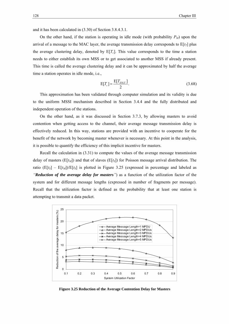
Chapter III
128
and it has been calculated in (3.30) of Section 3.8.4.3.1.
On the other hand, if the station is operating in idle mode (with probability PSI) upon the
arrival of a message to the MAC layer, the average transmission delay corresponds to E[tT] plus
the average clustering delay, denoted by E[Tc]. This value corresponds to the time a station
needs to either establish its own MSS or to get associated to another MSS if already present.
This time is called the average clustering delay and it can be approximated by half the average
time a station operates in idle mode, i.e.,
'E[ ]E[ ] .
2IDLE
c
TT (3.68)
This approximation has been validated through computer simulation and its validity is due
to the uniform MSSI mechanism described in Section 3.4.4 and the fully distributed and
independent operation of the stations.
On the other hand, as it was discussed in Section 3.7.3, by allowing masters to avoid
contention when getting access to the channel, their average message transmission delay is
effectively reduced. In this way, stations are provided with an incentive to cooperate for the
benefit of the network by becoming master whenever is necessary. At this point in the analysis,
it is possible to quantify the efficiency of this implicit incentive for masters.
Recall the calculation in (3.31) to compute the values of the average message transmission
delay of masters (E[tM]) and that of slaves (E[tS]) for Poisson message arrival distribution. The
ratio (E[tS] – E[tM])/E[tS] is plotted in Figure 3.25 (expressed in percentage and labeled as
“Reduction of the average delay for masters”) as a function of the utilization factor of the
system and for different message lengths (expressed in number of fragments per message).
Recall that the utilization factor is defined as the probability that at least one station is
attempting to transmit a data packet.
0
5
10
15
20
25
0.1 0.2 0.3 0.4 0.5 0.6 0.7 0.8 0.9
System Utilization Factor
Re
du
ctio
n o
f th
e a
vera
ge
de
lay
for
ma
ste
rs (
%)
Average Message Length=1 MPDUAverage Message Length=2 MPDUsAverage Message Length=3 MPDUsAverage Message Length=4 MPDUsAverage Message Length=5 MPDUs
Figure 3.25 Reduction of the Average Contention Delay for Masters
A Novel MAC Protocol: DQMAN
129
First, it is worth noting that since the ratio is always positive, the average transmission delay
of messages transmitted by a master is lower than that of slaves in all cases.
Second, the lower transmission delay perceived by masters strongly depends on the average
length of the data messages. The reason for this lies in the fact that the equations in (3.31)
contain the contributions of both the contention and the transmission times. Therefore, for short
message lengths (1 or 2 packets per message), when the contention time is comparable to the
effective data transmission time, DQMAN is very efficient in reducing the average transmission
delay for masters. For example, for an average message length of one packet, a master can
perceive an average transmission delay reduction of up to approximately 22% with respect to
that of slaves when the utilization factor is close to 0.5. On the contrary, as the average message
length grows, the contention time becomes very small compared to the actual data transmission
time, and accordingly, the reduction of the contention time becomes less relevant with respect to
the overall transmission delay.
Finally, it is important to pay attention to the fact that the curves in Figure 3.25 show a local
maximum. The probability that a master finds an empty minislot diminishes as the utilization
factor of the network grows. Note that the higher the utilization factor, the more access requests
will be transmitted per frame (in average).
Over a given threshold (which depends on the average message length), data transmissions
from the masters suffer from the latency required to find an empty minislot where to report a
successful slot. Under these conditions, the benefits obtained from the implicit cooperation
encouraging technique become smaller. However, as already mentioned, in all cases the average
delay of masters is always lower than that of slave stations. It is worth mentioning that the tree-
splitting nature of the collision resolution algorithm ensures access to masters regardless of the
traffic conditions.
3.8.4.7 Model Validation and Performance Evaluation
The accuracy of the proposed model of DQMAN for non-saturation traffic conditions is
assessed in this section. Results obtained with the analysis are compared to the ones obtained
through computer simulations using MACSWIN. Recall that simulations reproduce the
operation of the network and the rules of the clustering and MAC protocol without using any
mathematical expression for the MAC layer. It should be mentioned that the proposed model is
valid in steady state conditions, and thus all the analytical curves presented in this section are
valid as long as 1 . In the limit where 1 , the non-saturation model provides the same
results as the saturation model presented and evaluated in Section 3.8.3.
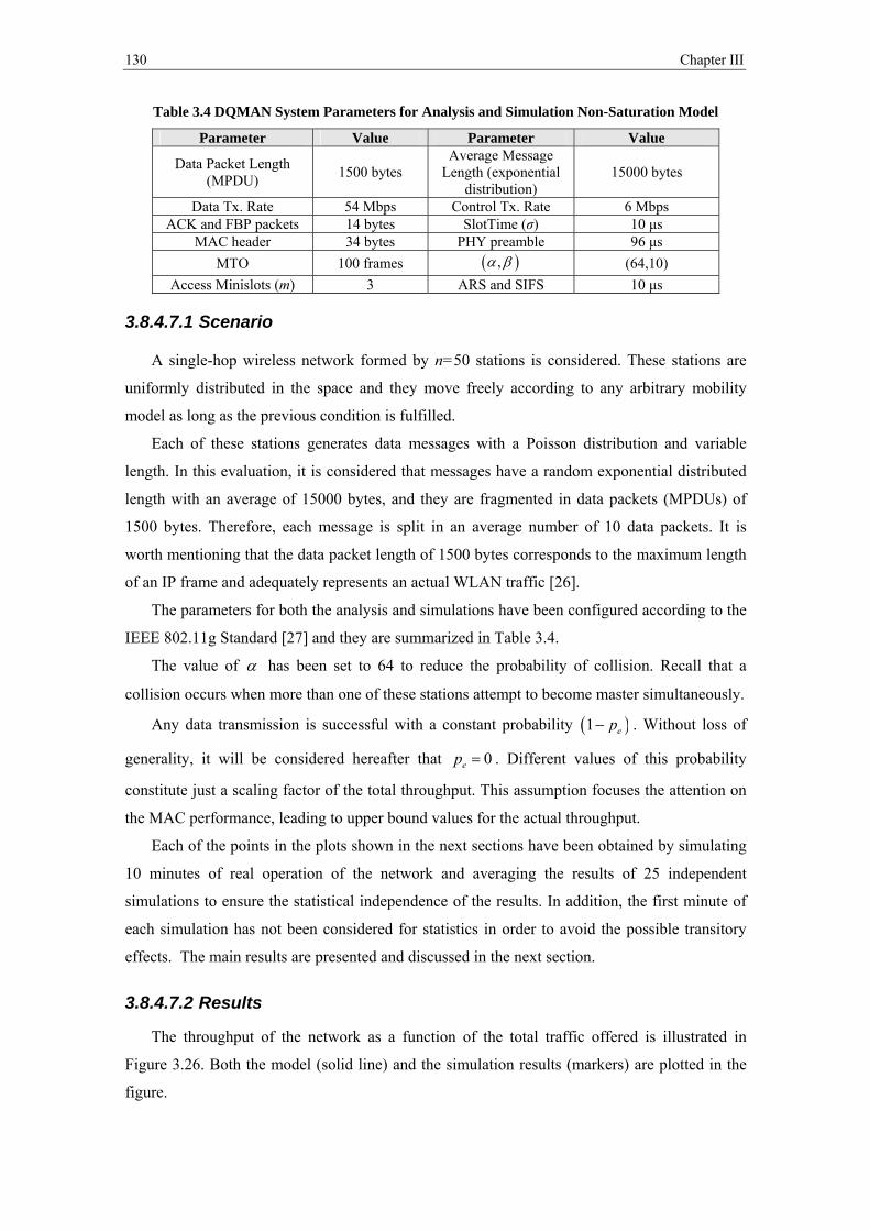
Chapter III
130
Table 3.4 DQMAN System Parameters for Analysis and Simulation Non-Saturation Model
Parameter Value Parameter Value
Data Packet Length (MPDU)
1500 bytes Average Message
Length (exponential distribution)
15000 bytes
Data Tx. Rate 54 Mbps Control Tx. Rate 6 Mbps ACK and FBP packets 14 bytes SlotTime (σ) 10 μs
MAC header 34 bytes PHY preamble 96 μs
MTO 100 frames , (64,10)
Access Minislots (m) 3 ARS and SIFS 10 μs
3.8.4.7.1 Scenario
A single-hop wireless network formed by n=50 stations is considered. These stations are
uniformly distributed in the space and they move freely according to any arbitrary mobility
model as long as the previous condition is fulfilled.
Each of these stations generates data messages with a Poisson distribution and variable
length. In this evaluation, it is considered that messages have a random exponential distributed
length with an average of 15000 bytes, and they are fragmented in data packets (MPDUs) of
1500 bytes. Therefore, each message is split in an average number of 10 data packets. It is
worth mentioning that the data packet length of 1500 bytes corresponds to the maximum length
of an IP frame and adequately represents an actual WLAN traffic [26].
The parameters for both the analysis and simulations have been configured according to the
IEEE 802.11g Standard [27] and they are summarized in Table 3.4.
The value of has been set to 64 to reduce the probability of collision. Recall that a
collision occurs when more than one of these stations attempt to become master simultaneously.
Any data transmission is successful with a constant probability 1 ep . Without loss of
generality, it will be considered hereafter that 0ep . Different values of this probability
constitute just a scaling factor of the total throughput. This assumption focuses the attention on
the MAC performance, leading to upper bound values for the actual throughput.
Each of the points in the plots shown in the next sections have been obtained by simulating
10 minutes of real operation of the network and averaging the results of 25 independent
simulations to ensure the statistical independence of the results. In addition, the first minute of
each simulation has not been considered for statistics in order to avoid the possible transitory
effects. The main results are presented and discussed in the next section.
3.8.4.7.2 Results
The throughput of the network as a function of the total traffic offered is illustrated in
Figure 3.26. Both the model (solid line) and the simulation results (markers) are plotted in the
figure.
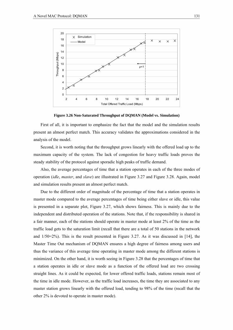
A Novel MAC Protocol: DQMAN
131
0
2
4
6
8
10
12
14
16
18
20
2 4 6 8 10 12 14 16 18 20 22 24
Total Offered Traffic Load (Mbps)
Th
rou
gh
pu
t (M
bp
s)
Simulation
Model
ρ<1
Figure 3.26 Non-Saturated Throughput of DQMAN (Model vs. Simulation)
First of all, it is important to emphasize the fact that the model and the simulation results
present an almost perfect match. This accuracy validates the approximations considered in the
analysis of the model.
Second, it is worth noting that the throughput grows linearly with the offered load up to the
maximum capacity of the system. The lack of congestion for heavy traffic loads proves the
steady stability of the protocol against sporadic high peaks of traffic demand.
Also, the average percentages of time that a station operates in each of the three modes of
operation (idle, master, and slave) are illustrated in Figure 3.27 and Figure 3.28. Again, model
and simulation results present an almost perfect match.
Due to the different order of magnitude of the percentage of time that a station operates in
master mode compared to the average percentages of time being either slave or idle, this value
is presented in a separate plot, Figure 3.27, which shows fairness. This is mainly due to the
independent and distributed operation of the stations. Note that, if the responsibility is shared in
a fair manner, each of the stations should operate in master mode at least 2% of the time as the
traffic load gets to the saturation limit (recall that there are a total of 50 stations in the network
and 1/50=2%). This is the result presented in Figure 3.27. As it was discussed in [14], the
Master Time Out mechanism of DQMAN ensures a high degree of fairness among users and
thus the variance of this average time operating in master mode among the different stations is
minimized. On the other hand, it is worth seeing in Figure 3.28 that the percentages of time that
a station operates in idle or slave mode as a function of the offered load are two crossing
straight lines. As it could be expected, for lower offered traffic loads, stations remain most of
the time in idle mode. However, as the traffic load increases, the time they are associated to any
master station grows linearly with the offered load, tending to 98% of the time (recall that the
other 2% is devoted to operate in master mode).
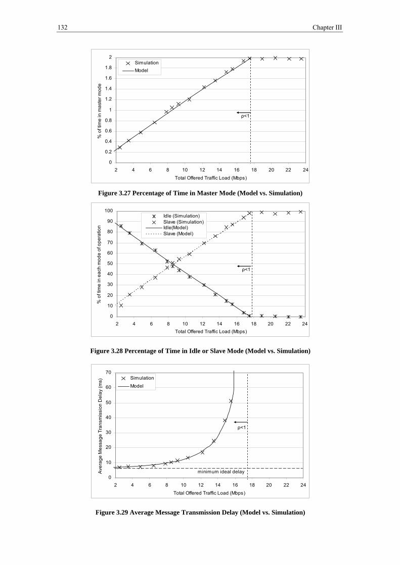
Chapter III
132
0
0.2
0.4
0.6
0.8
1
1.2
1.4
1.6
1.8
2
2 4 6 8 10 12 14 16 18 20 22 24
Total Offered Traffic Load (Mbps)
% o
f tim
e in
ma
ste
r m
od
e
Simulation
Model
ρ<1
Figure 3.27 Percentage of Time in Master Mode (Model vs. Simulation)
0
10
20
30
40
50
60
70
80
90
100
2 4 6 8 10 12 14 16 18 20 22 24
Total Offered Traffic Load (Mbps)
% o
f tim
e in
ea
ch m
od
e o
f op
era
tion
Idle (Simulation)Slave (Simulation)Idle(Model)Slave (Model)
ρ<1
Figure 3.28 Percentage of Time in Idle or Slave Mode (Model vs. Simulation)
0
10
20
30
40
50
60
70
2 4 6 8 10 12 14 16 18 20 22 24
Total Offered Traffic Load (Mbps)
Ave
rag
e M
ess
ag
e T
ran
smis
sio
n D
ela
y (m
s)
Simulation
Model
ρ<1
minimum ideal delay
Figure 3.29 Average Message Transmission Delay (Model vs. Simulation)
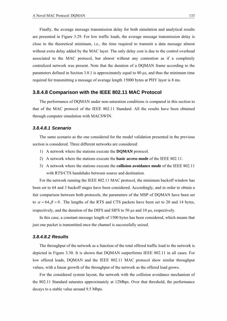
A Novel MAC Protocol: DQMAN
133
Finally, the average message transmission delay for both simulation and analytical results
are presented in Figure 3.29. For low traffic loads, the average message transmission delay is
close to the theoretical minimum, i.e., the time required to transmit a data message almost
without extra delay added by the MAC layer. The only delay cost is due to the control overhead
associated to the MAC protocol, but almost without any contention as if a completely
centralized network was present. Note that the duration of a DQMAN frame according to the
parameters defined in Section 3.8.1 is approximately equal to 80 µs, and thus the minimum time
required for transmitting a message of average length 15000 bytes at PHY layer is 8 ms.
3.8.4.8 Comparison with the IEEE 802.11 MAC Protocol
The performance of DQMAN under non-saturation conditions is compared in this section to
that of the MAC protocol of the IEEE 802.11 Standard. All the results have been obtained
through computer simulation with MACSWIN.
3.8.4.8.1 Scenario
The same scenario as the one considered for the model validation presented in the previous
section is considered. Three different networks are considered:
1) A network where the stations execute the DQMAN protocol.
2) A network where the stations execute the basic access mode of the IEEE 802.11.
3) A network where the stations execute the collision avoidance mode of the IEEE 802.11
with RTS/CTS handshake between source and destination.
For the network running the IEEE 802.11 MAC protocol, the minimum backoff window has
been set to 64 and 3 backoff stages have been considered. Accordingly, and in order to obtain a
fair comparison between both protocols, the parameters of the MSP of DQMAN have been set
to 64, 0 . The lengths of the RTS and CTS packets have been set to 20 and 14 bytes,
respectively, and the duration of the DIFS and SIFS to 50 µs and 10 µs, respectively.
In this case, a constant message length of 1500 bytes has been considered, which means that
just one packet is transmitted once the channel is successfully seized.
3.8.4.8.2 Results
The throughput of the network as a function of the total offered traffic load to the network is
depicted in Figure 3.30. It is shown that DQMAN outperforms IEEE 802.11 in all cases. For
low offered loads, DQMAN and the IEEE 802.11 MAC protocol show similar throughput
values, with a linear growth of the throughput of the network as the offered load grows.
For the considered system layout, the network with the collision avoidance mechanism of
the 802.11 Standard saturates approximately at 12Mbps. Over that threshold, the performance
decays to a stable value around 9.5 Mbps.
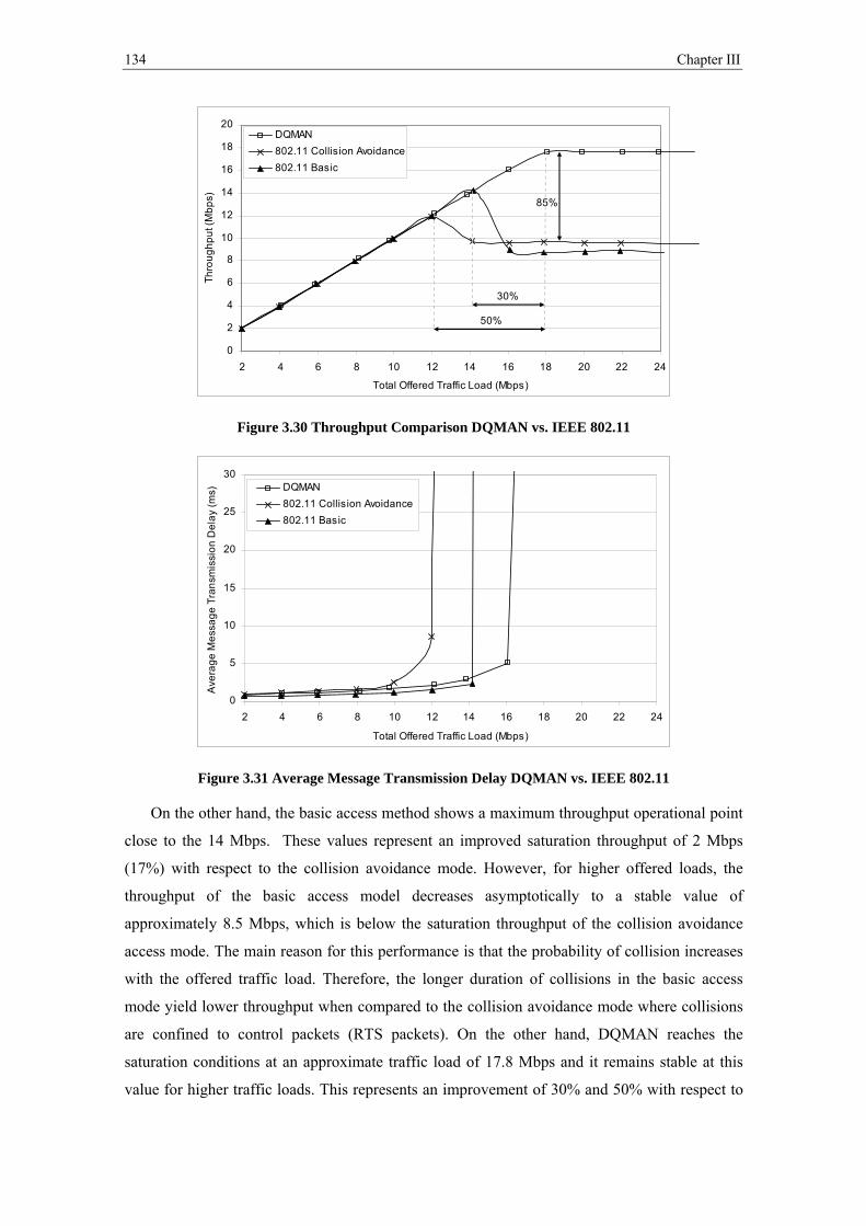
Chapter III
134
0
2
4
6
8
10
12
14
16
18
20
2 4 6 8 10 12 14 16 18 20 22 24
Total Offered Traffic Load (Mbps)
Th
rou
gh
pu
t (M
bp
s)
DQMAN
802.11 Collision Avoidance
802.11 Basic
85%
30%
50%
Figure 3.30 Throughput Comparison DQMAN vs. IEEE 802.11
0
5
10
15
20
25
30
2 4 6 8 10 12 14 16 18 20 22 24
Total Offered Traffic Load (Mbps)
Ave
rag
e M
ess
ag
e T
ran
smis
sio
n D
ela
y (m
s) DQMAN
802.11 Collision Avoidance
802.11 Basic
Figure 3.31 Average Message Transmission Delay DQMAN vs. IEEE 802.11
On the other hand, the basic access method shows a maximum throughput operational point
close to the 14 Mbps. These values represent an improved saturation throughput of 2 Mbps
(17%) with respect to the collision avoidance mode. However, for higher offered loads, the
throughput of the basic access model decreases asymptotically to a stable value of
approximately 8.5 Mbps, which is below the saturation throughput of the collision avoidance
access mode. The main reason for this performance is that the probability of collision increases
with the offered traffic load. Therefore, the longer duration of collisions in the basic access
mode yield lower throughput when compared to the collision avoidance mode where collisions
are confined to control packets (RTS packets). On the other hand, DQMAN reaches the
saturation conditions at an approximate traffic load of 17.8 Mbps and it remains stable at this
value for higher traffic loads. This represents an improvement of 30% and 50% with respect to
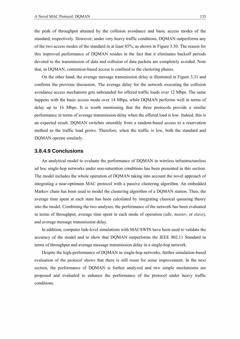
A Novel MAC Protocol: DQMAN
135
the peak of throughput attained by the collision avoidance and basic access modes of the
standard, respectively. However, under very heavy traffic conditions, DQMAN outperforms any
of the two access modes of the standard in at least 85%, as shown in Figure 3.30. The reason for
this improved performance of DQMAN resides in the fact that it eliminates backoff periods
devoted to the transmission of data and collision of data packets are completely avoided. Note
that, in DQMAN, contention-based access is confined to the clustering phases.
On the other hand, the average message transmission delay is illustrated in Figure 3.31 and
confirms the previous discussion. The average delay for the network executing the collision
avoidance access mechanism gets unbounded for offered traffic loads over 12 Mbps. The same
happens with the basic access mode over 14 Mbps, while DQMAN performs well in terms of
delay up to 16 Mbps. It is worth mentioning that the three protocols provide a similar
performance in terms of average transmission delay when the offered load is low. Indeed, this is
an expected result. DQMAN switches smoothly from a random-based access to a reservation
method as the traffic load grows. Therefore, when the traffic is low, both the standard and
DQMAN operate similarly.
3.8.4.9 Conclusions
An analytical model to evaluate the performance of DQMAN in wireless infrastructureless
ad hoc single-hop networks under non-saturation conditions has been presented in this section.
The model includes the whole operation of DQMAN taking into account the novel approach of
integrating a near-optimum MAC protocol with a passive clustering algorithm. An embedded
Markov chain has been used to model the clustering algorithm of a DQMAN station. Then, the
average time spent at each state has been calculated by integrating classical queueing theory
into the model. Combining the two analyses, the performance of the network has been evaluated
in terms of throughput, average time spent in each mode of operation (idle, master, or slave),
and average message transmission delay.
In addition, computer link-level simulations with MACSWIN have been used to validate the
accuracy of the model and to show that DQMAN outperforms the IEEE 802.11 Standard in
terms of throughput and average message transmission delay in a single-hop network.
Despite the high-performance of DQMAN in single-hop networks, further simulation-based
evaluation of the protocol shows that there is still room for some improvement. In the next
section, the performance of DQMAN is further analyzed and two simple mechanisms are
proposed and evaluated to enhance the performance of the protocol under heavy traffic
conditions.
Chapter III
136
3.9 Performance Enhancements
3.9.1 Introduction
As was shown in the previous two sections, the performance of DQMAN in single-hop
networks is stable for any offered traffic load and almost independent of the number of stations
loading the network. The protocol avoids collisions of data packets and confines contention to
only clustering processes and a small part of the MAC frame.
Despite the good performance of the protocol, further analysis shows that there is still room
for improvement under heavy traffic conditions. Two simple mechanisms are presented in this
section to improve the performance of DQMAN under heavy traffic conditions. They are the
Master Cooperation Request (MCR) and the Advanced MTO mechanisms, and they are
described in Sections 3.9.2 and 3.9.3, respectively. The performance of DQMAN with these two
mechanisms is evaluated through computer simulation in Section 3.9.4. Finally, Section 3.9.5
concludes the section and gives some final remarks.
3.9.2 Master Cooperation Request (MCR)
3.9.2.1 Problem Statement
The MTO mechanism described in Section 3.4.6 ensures that the responsibility of becoming
master is shared in a fair manner among the different stations of a network under heavy traffic
conditions (saturation conditions). Without the MTO mechanism and under high traffic loads,
once a station becomes master, it would operate as such indefinitely since there would be
always a packet ready to be transmitted.
However, upon the execution of a MTO, a re-clustering phase is initiated. All the stations of
the network with data to transmit set up their MSSI counter according to the algorithm
presented in Section 3.4.4 and initiate a countdown. As explained in that section, the MSSI is
composed of the sum of two components with fixed and random durations. While the first
component is required to minimize the probability that a station is set to master mode twice
consecutively (see Section 3.8.3.3), the second is required to avoid collisions among stations
attempting to become master simultaneously.
This operation leads to backoff deferral periods necessary for the proper set up of a new
cluster upon the breakage of the current cluster. During these periods, the channel is not used
and the stations with data to transmit contend to become master. Therefore, collisions among
different stations attempting to become master simultaneously may also occur. In addition, there
is a non-zero probability that a given station is set to master mode twice consecutively.
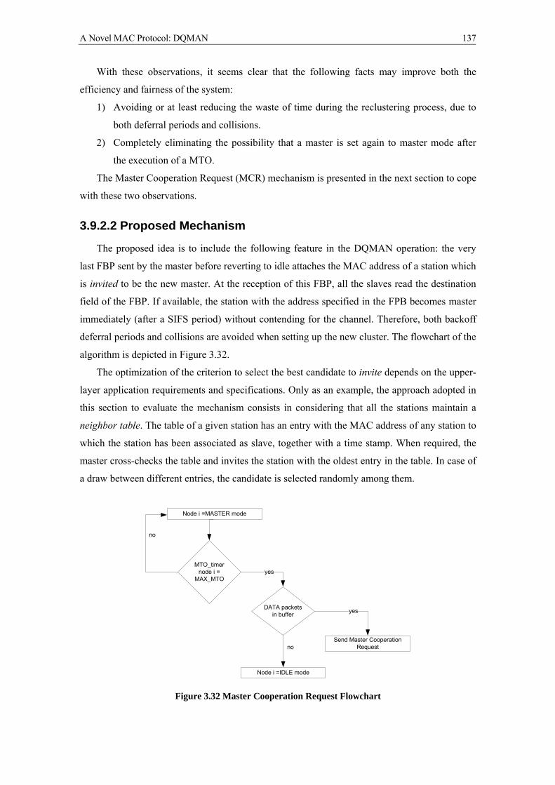
A Novel MAC Protocol: DQMAN
137
With these observations, it seems clear that the following facts may improve both the
efficiency and fairness of the system:
1) Avoiding or at least reducing the waste of time during the reclustering process, due to
both deferral periods and collisions.
2) Completely eliminating the possibility that a master is set again to master mode after
the execution of a MTO.
The Master Cooperation Request (MCR) mechanism is presented in the next section to cope
with these two observations.
3.9.2.2 Proposed Mechanism
The proposed idea is to include the following feature in the DQMAN operation: the very
last FBP sent by the master before reverting to idle attaches the MAC address of a station which
is invited to be the new master. At the reception of this FBP, all the slaves read the destination
field of the FBP. If available, the station with the address specified in the FPB becomes master
immediately (after a SIFS period) without contending for the channel. Therefore, both backoff
deferral periods and collisions are avoided when setting up the new cluster. The flowchart of the
algorithm is depicted in Figure 3.32.
The optimization of the criterion to select the best candidate to invite depends on the upper-
layer application requirements and specifications. Only as an example, the approach adopted in
this section to evaluate the mechanism consists in considering that all the stations maintain a
neighbor table. The table of a given station has an entry with the MAC address of any station to
which the station has been associated as slave, together with a time stamp. When required, the
master cross-checks the table and invites the station with the oldest entry in the table. In case of
a draw between different entries, the candidate is selected randomly among them.
yes
yes
Node i =MASTER mode
MTO_timer node i =
MAX_MTO
DATA packets in buffer
Node i =IDLE mode
noSend Master Cooperation
Request
no
Figure 3.32 Master Cooperation Request Flowchart
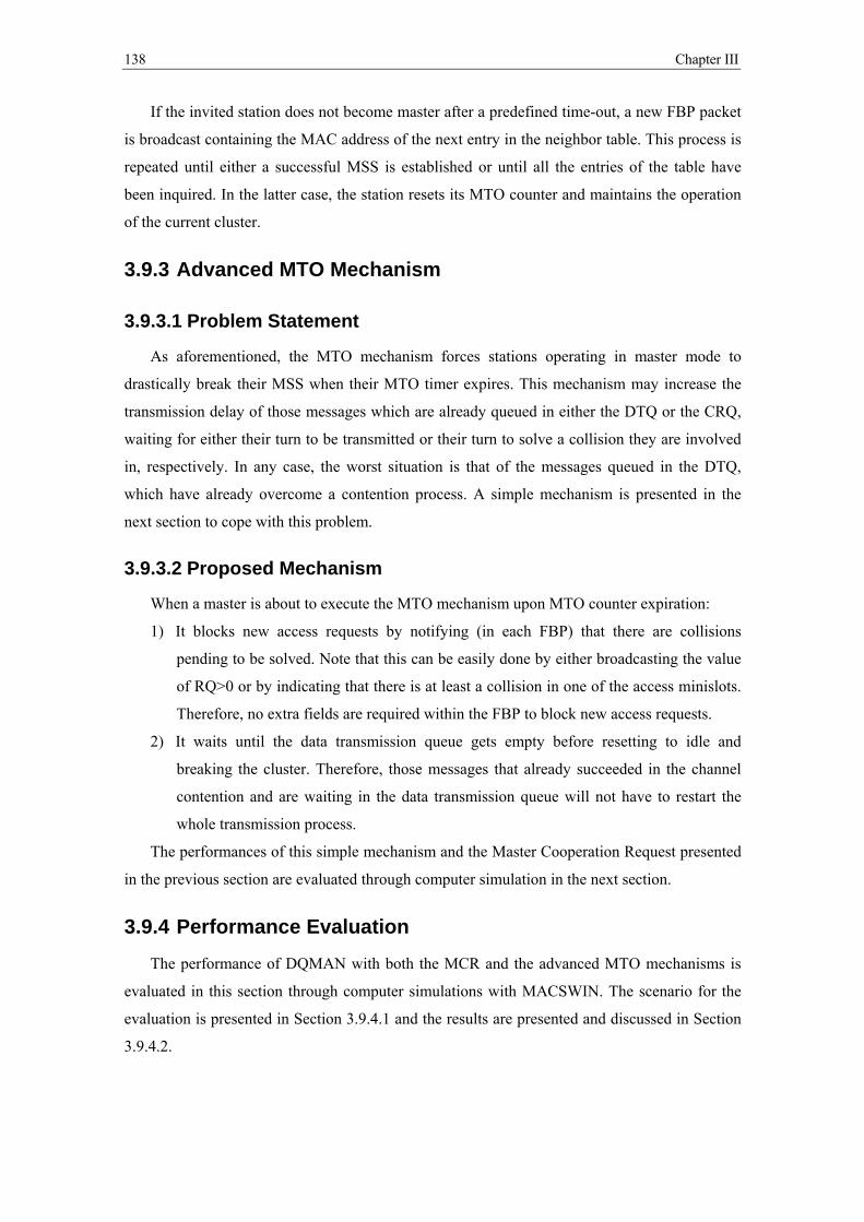
Chapter III
138
If the invited station does not become master after a predefined time-out, a new FBP packet
is broadcast containing the MAC address of the next entry in the neighbor table. This process is
repeated until either a successful MSS is established or until all the entries of the table have
been inquired. In the latter case, the station resets its MTO counter and maintains the operation
of the current cluster.
3.9.3 Advanced MTO Mechanism
3.9.3.1 Problem Statement
As aforementioned, the MTO mechanism forces stations operating in master mode to
drastically break their MSS when their MTO timer expires. This mechanism may increase the
transmission delay of those messages which are already queued in either the DTQ or the CRQ,
waiting for either their turn to be transmitted or their turn to solve a collision they are involved
in, respectively. In any case, the worst situation is that of the messages queued in the DTQ,
which have already overcome a contention process. A simple mechanism is presented in the
next section to cope with this problem.
3.9.3.2 Proposed Mechanism
When a master is about to execute the MTO mechanism upon MTO counter expiration:
1) It blocks new access requests by notifying (in each FBP) that there are collisions
pending to be solved. Note that this can be easily done by either broadcasting the value
of RQ>0 or by indicating that there is at least a collision in one of the access minislots.
Therefore, no extra fields are required within the FBP to block new access requests.
2) It waits until the data transmission queue gets empty before resetting to idle and
breaking the cluster. Therefore, those messages that already succeeded in the channel
contention and are waiting in the data transmission queue will not have to restart the
whole transmission process.
The performances of this simple mechanism and the Master Cooperation Request presented
in the previous section are evaluated through computer simulation in the next section.
3.9.4 Performance Evaluation
The performance of DQMAN with both the MCR and the advanced MTO mechanisms is
evaluated in this section through computer simulations with MACSWIN. The scenario for the
evaluation is presented in Section 3.9.4.1 and the results are presented and discussed in Section
3.9.4.2.
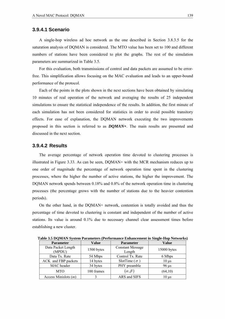
A Novel MAC Protocol: DQMAN
139
3.9.4.1 Scenario
A single-hop wireless ad hoc network as the one described in Section 3.8.3.5 for the
saturation analysis of DQMAN is considered. The MTO value has been set to 100 and different
numbers of stations have been considered to plot the graphs. The rest of the simulation
parameters are summarized in Table 3.5.
For this evaluation, both transmissions of control and data packets are assumed to be error-
free. This simplification allows focusing on the MAC evaluation and leads to an upper-bound
performance of the protocol.
Each of the points in the plots shown in the next sections have been obtained by simulating
10 minutes of real operation of the network and averaging the results of 25 independent
simulations to ensure the statistical independence of the results. In addition, the first minute of
each simulation has not been considered for statistics in order to avoid possible transitory
effects. For ease of explanation, the DQMAN network executing the two improvements
proposed in this section is referred to as DQMAN+. The main results are presented and
discussed in the next section.
3.9.4.2 Results
The average percentage of network operation time devoted to clustering processes is
illustrated in Figure 3.33. As can be seen, DQMAN+ with the MCR mechanism reduces up to
one order of magnitude the percentage of network operation time spent in the clustering
processes, where the higher the number of active stations, the higher the improvement. The
DQMAN network spends between 0.18% and 0.8% of the network operation time in clustering
processes (the percentage grows with the number of stations due to the heavier contention
periods).
On the other hand, in the DQMAN+ network, contention is totally avoided and thus the
percentage of time devoted to clustering is constant and independent of the number of active
stations. Its value is around 0.1% due to necessary channel clear assessment times before
establishing a new cluster.
Table 3.5 DQMAN System Parameters (Performance Enhancement in Single-Hop Networks) Parameter Value Parameter Value
Data Packet Length (MPDU)
1500 bytes Constant Message
Length 15000 bytes
Data Tx. Rate 54 Mbps Control Tx. Rate 6 Mbps ACK and FBP packets 14 bytes SlotTime ( ) 10 μs
MAC header 34 bytes PHY preamble 96 μs
MTO 100 frames , (64,10)
Access Minislots (m) 3 ARS and SIFS 10 μs
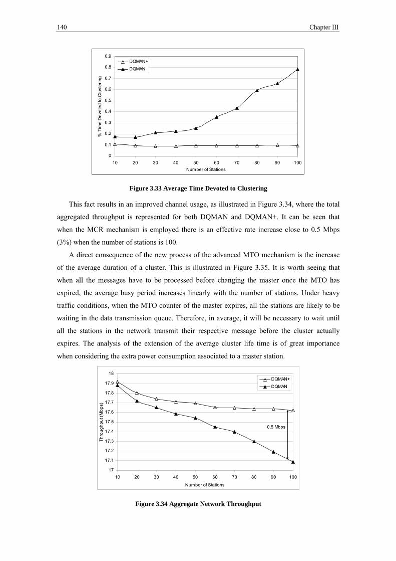
Chapter III
140
0
0.1
0.2
0.3
0.4
0.5
0.6
0.7
0.8
0.9
10 20 30 40 50 60 70 80 90 100
Number of Stations
% T
ime
De
vote
d to
Clu
ste
rin
g
DQMAN+
DQMAN
Figure 3.33 Average Time Devoted to Clustering
This fact results in an improved channel usage, as illustrated in Figure 3.34, where the total
aggregated throughput is represented for both DQMAN and DQMAN+. It can be seen that
when the MCR mechanism is employed there is an effective rate increase close to 0.5 Mbps
(3%) when the number of stations is 100.
A direct consequence of the new process of the advanced MTO mechanism is the increase
of the average duration of a cluster. This is illustrated in Figure 3.35. It is worth seeing that
when all the messages have to be processed before changing the master once the MTO has
expired, the average busy period increases linearly with the number of stations. Under heavy
traffic conditions, when the MTO counter of the master expires, all the stations are likely to be
waiting in the data transmission queue. Therefore, in average, it will be necessary to wait until
all the stations in the network transmit their respective message before the cluster actually
expires. The analysis of the extension of the average cluster life time is of great importance
when considering the extra power consumption associated to a master station.
17
17.1
17.2
17.3
17.4
17.5
17.6
17.7
17.8
17.9
18
10 20 30 40 50 60 70 80 90 100
Number of Stations
Th
rou
gh
pu
t (M
bp
s)
DQMAN+
DQMAN
0.5 Mbps
Figure 3.34 Aggregate Network Throughput
A Novel MAC Protocol: DQMAN
141
0
200
400
600
800
1000
1200
10 20 30 40 50 60 70 80 90 100
Number of Stations
Ave
rag
e C
lust
er
Life
-Tim
e (
DQ
MA
N F
ram
es) DQMAN+
DQMAN
Figure 3.35 Average Duration of a Master Busy Period
On the other hand, DQMAN+ shows in Figure 3.36 just a slightly better performance in
terms of average message transmission delay with respect to DQMAN. This improved
performance is due to the reduction of the time devoted to contention in the network thanks to
the MCR mechanism. Therefore, the relative enhanced performance grows with the number of
active stations in the network as the contention becomes harder.
It is worth mentioning that although one may expect that the advanced MTO mechanism
provides better performance in terms of average message transmission delay, results show that
the improved performance is attained in terms of the variance of the delay, but not in average
terms. In order to illustrate this, the Jain Index (JI) [30] of the average message transmission
delay is plotted in Figure 3.37. Given i=1,..,N samples of a random variable Ti, the JI is
computed as
2
2,
iN
iN
T
JIN T
(3.69)
and it has a value within the interval [0,1]. The less variance between the N samples, the more
close to 1 the JI is. Therefore, the value of the JI provides a very intuitive figure of the fairness
of any random process. As it can be seen in Figure 3.37, DQMAN+ attains a more flat response
of the network to the average message transmission delay. With the advanced MTO mechanism,
all those messages which have already overcome a contention process do not have to restart
from scratch whenever a MTO is executed. However, all those new messages that are blocked
until the entire DTQ is processed suffer latency in the access to the channel. The result is an
improved fairness, but similar results in average terms.
A summary of the contents of this section and the most relevant conclusions are presented
in the next section.
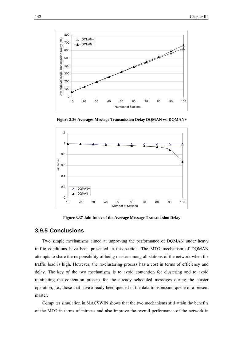
Chapter III
142
0
100
200
300
400
500
600
700
800
10 20 30 40 50 60 70 80 90 100
Number of Stations
Ave
rag
e M
ess
ag
e T
ran
smis
sio
n D
ela
y (m
s) DQMAN+
DQMAN
Figure 3.36 Averages Message Transmission Delay DQMAN vs. DQMAN+
0
0.2
0.4
0.6
0.8
1
1.2
10 20 30 40 50 60 70 80 90 100Number of Stations
Jain
Ind
ex
DQMAN+
DQMAN
Figure 3.37 Jain Index of the Average Message Transmission Delay
3.9.5 Conclusions
Two simple mechanisms aimed at improving the performance of DQMAN under heavy
traffic conditions have been presented in this section. The MTO mechanism of DQMAN
attempts to share the responsibility of being master among all stations of the network when the
traffic load is high. However, the re-clustering process has a cost in terms of efficiency and
delay. The key of the two mechanisms is to avoid contention for clustering and to avoid
reinitiating the contention process for the already scheduled messages during the cluster
operation, i.e., those that have already been queued in the data transmission queue of a present
master.
Computer simulation in MACSWIN shows that the two mechanisms still attain the benefits
of the MTO in terms of fairness and also improve the overall performance of the network in
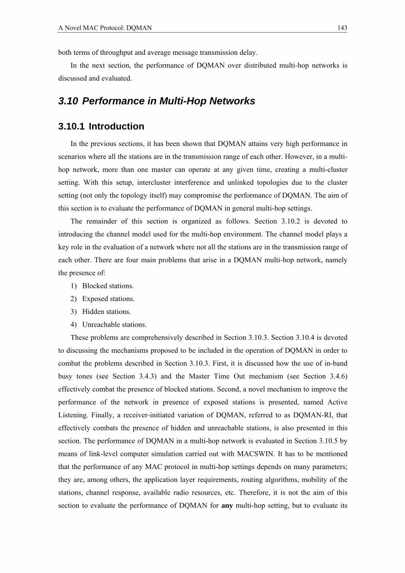
A Novel MAC Protocol: DQMAN
143
both terms of throughput and average message transmission delay.
In the next section, the performance of DQMAN over distributed multi-hop networks is
discussed and evaluated.
3.10 Performance in Multi-Hop Networks
3.10.1 Introduction
In the previous sections, it has been shown that DQMAN attains very high performance in
scenarios where all the stations are in the transmission range of each other. However, in a multi-
hop network, more than one master can operate at any given time, creating a multi-cluster
setting. With this setup, intercluster interference and unlinked topologies due to the cluster
setting (not only the topology itself) may compromise the performance of DQMAN. The aim of
this section is to evaluate the performance of DQMAN in general multi-hop settings.
The remainder of this section is organized as follows. Section 3.10.2 is devoted to
introducing the channel model used for the multi-hop environment. The channel model plays a
key role in the evaluation of a network where not all the stations are in the transmission range of
each other. There are four main problems that arise in a DQMAN multi-hop network, namely
the presence of:
1) Blocked stations.
2) Exposed stations.
3) Hidden stations.
4) Unreachable stations.
These problems are comprehensively described in Section 3.10.3. Section 3.10.4 is devoted
to discussing the mechanisms proposed to be included in the operation of DQMAN in order to
combat the problems described in Section 3.10.3. First, it is discussed how the use of in-band
busy tones (see Section 3.4.3) and the Master Time Out mechanism (see Section 3.4.6)
effectively combat the presence of blocked stations. Second, a novel mechanism to improve the
performance of the network in presence of exposed stations is presented, named Active
Listening. Finally, a receiver-initiated variation of DQMAN, referred to as DQMAN-RI, that
effectively combats the presence of hidden and unreachable stations, is also presented in this
section. The performance of DQMAN in a multi-hop network is evaluated in Section 3.10.5 by
means of link-level computer simulation carried out with MACSWIN. It has to be mentioned
that the performance of any MAC protocol in multi-hop settings depends on many parameters;
they are, among others, the application layer requirements, routing algorithms, mobility of the
stations, channel response, available radio resources, etc. Therefore, it is not the aim of this
section to evaluate the performance of DQMAN for any multi-hop setting, but to evaluate its
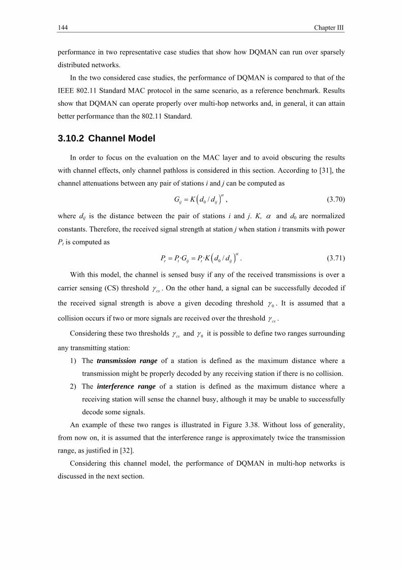
Chapter III
144
performance in two representative case studies that show how DQMAN can run over sparsely
distributed networks.
In the two considered case studies, the performance of DQMAN is compared to that of the
IEEE 802.11 Standard MAC protocol in the same scenario, as a reference benchmark. Results
show that DQMAN can operate properly over multi-hop networks and, in general, it can attain
better performance than the 802.11 Standard.
3.10.2 Channel Model
In order to focus on the evaluation on the MAC layer and to avoid obscuring the results
with channel effects, only channel pathloss is considered in this section. According to [31], the
channel attenuations between any pair of stations i and j can be computed as
0 / ,ij ijG K d d
(3.70)
where dij is the distance between the pair of stations i and j. K, and d0 are normalized
constants. Therefore, the received signal strength at station j when station i transmits with power
Pt is computed as
0· · / .r t ij t ijP P G P K d d
(3.71)
With this model, the channel is sensed busy if any of the received transmissions is over a
carrier sensing (CS) threshold cs . On the other hand, a signal can be successfully decoded if
the received signal strength is above a given decoding threshold 0 . It is assumed that a
collision occurs if two or more signals are received over the threshold cs .
Considering these two thresholds cs and 0 it is possible to define two ranges surrounding
any transmitting station:
1) The transmission range of a station is defined as the maximum distance where a
transmission might be properly decoded by any receiving station if there is no collision.
2) The interference range of a station is defined as the maximum distance where a
receiving station will sense the channel busy, although it may be unable to successfully
decode some signals.
An example of these two ranges is illustrated in Figure 3.38. Without loss of generality,
from now on, it is assumed that the interference range is approximately twice the transmission
range, as justified in [32].
Considering this channel model, the performance of DQMAN in multi-hop networks is
discussed in the next section.
A Novel MAC Protocol: DQMAN
145
Transmission range
Interference range
Figure 3.38 Transmission and Interference Ranges
3.10.3 Performance Discussion
Four problems arise in a multi-hop network where DQMAN is executed at the MAC layer.
They are the presence of:
1) Blocked stations.
2) Exposed stations (from a cluster point of view).
3) Hidden stations (from a cluster point of view).
4) Unreachable stations.
The four problems are comprehensively described in the following sections. It is important
to emphasize that these problems are interrelated with each other and occur simultaneously in a
network. This combination of factors, together with the variability of the radio channel, makes
the theoretical analysis of DQMAN in multi-hop networks an extremely hard task, and
constitutes the main rationale for the computer-based evaluation presented in this section.
3.10.3.1 Blocked Stations
In a DQMAN network, a station which lies in the transmission range of more than one
master simultaneously receives different FBP from different masters. This situation can either
lead to a ping-pong effect between the involved masters or cause the impossibility of the station
to get associated to any of them.
This problem is illustrated in Figure 3.39 where station S1 is able to receive the FBP from
both M1 and M2. As a consequence, it is unable to get associated to any of the MSS.
Normally these stations cannot take part in the communications of any of the involved
clusters and they are called blocked stations. The presence of stations unable to take part in the
communications may reduce the overall channel usage efficiency. For example, since the data
packets transmitted to any of these stations will not be acknowledged, retransmissions will be
scheduled and the overall network traffic load will be increased.
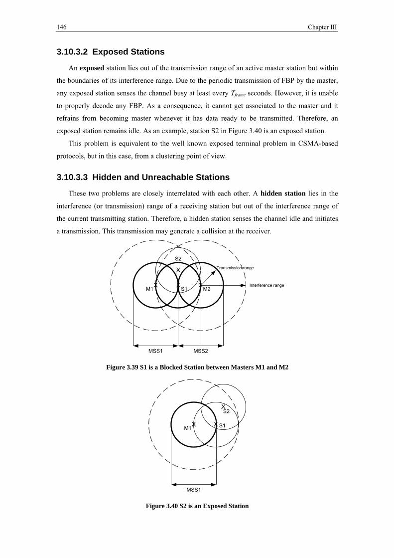
Chapter III
146
3.10.3.2 Exposed Stations
An exposed station lies out of the transmission range of an active master station but within
the boundaries of its interference range. Due to the periodic transmission of FBP by the master,
any exposed station senses the channel busy at least every Tframe seconds. However, it is unable
to properly decode any FBP. As a consequence, it cannot get associated to the master and it
refrains from becoming master whenever it has data ready to be transmitted. Therefore, an
exposed station remains idle. As an example, station S2 in Figure 3.40 is an exposed station.
This problem is equivalent to the well known exposed terminal problem in CSMA-based
protocols, but in this case, from a clustering point of view.
3.10.3.3 Hidden and Unreachable Stations
These two problems are closely interrelated with each other. A hidden station lies in the
interference (or transmission) range of a receiving station but out of the interference range of
the current transmitting station. Therefore, a hidden station senses the channel idle and initiates
a transmission. This transmission may generate a collision at the receiver.
X X
MSS2MSS1
M1 M2S1X
X
S2
Transmission range
Interference range
Figure 3.39 S1 is a Blocked Station between Masters M1 and M2
X
MSS1
M1 S1X
XS2
Figure 3.40 S2 is an Exposed Station
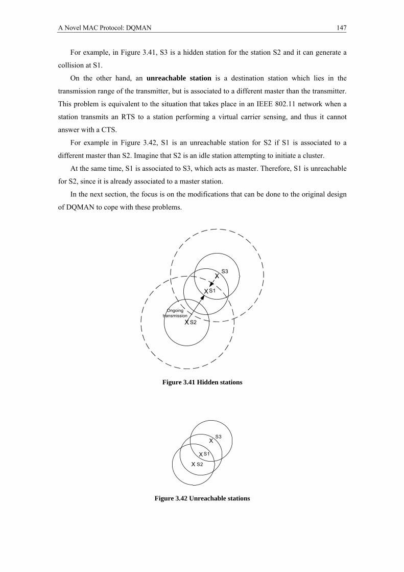
A Novel MAC Protocol: DQMAN
147
For example, in Figure 3.41, S3 is a hidden station for the station S2 and it can generate a
collision at S1.
On the other hand, an unreachable station is a destination station which lies in the
transmission range of the transmitter, but is associated to a different master than the transmitter.
This problem is equivalent to the situation that takes place in an IEEE 802.11 network when a
station transmits an RTS to a station performing a virtual carrier sensing, and thus it cannot
answer with a CTS.
For example in Figure 3.42, S1 is an unreachable station for S2 if S1 is associated to a
different master than S2. Imagine that S2 is an idle station attempting to initiate a cluster.
At the same time, S1 is associated to S3, which acts as master. Therefore, S1 is unreachable
for S2, since it is already associated to a master station.
In the next section, the focus is on the modifications that can be done to the original design
of DQMAN to cope with these problems.
S1
XS3
X S2
X
Ongoing transmission
Figure 3.41 Hidden stations
S1
XS3
X S2
X
Figure 3.42 Unreachable stations
Chapter III
148
3.10.4 Modifications for Multi-hop Networks
Considering the challenges posed by the multi-hop environment described in the previous
section, this section aims at discussing the mechanisms proposed to be included in DQMAN to
combat the presence of blocked, exposed, hidden, and unreachable stations.
In Section 3.10.4.1, it is discussed the role of busy tones and the MTO mechanism in
combating with the presence of blocked stations. Then, the Active Listening mechanism is
presented in Section 0 as a solution to combat the presence of exposed stations. Finally, the
receiver initiated clustering mechanism is presented in Section 3.10.4.3 to combat the presence
of hidden and unreachable stations.
In fact, all these mechanisms work together to enable the operation of DQMAN in multi-
hop settings, as it will be shown in Section 3.10.5, where the results of link-level computer
simulations are presented.
3.10.4.1 Tackling with Blocked Stations: Busy Tones and MTO
The problem of the blocked stations can be eliminated if a minimum distance of three hops
(counted in terms of transmission range units) is left between simultaneous operating masters
[33].
Indeed, the already existing in-band busy tones (BTs) of DQMAN act as an implicit
protection against this problem. They attempt to ensure a minimum distance of three-hops
between masters. As it was explained in Section 3.3, every slave in an MSS is responsible for
transmitting an in-band busy tone (BT) upon the reception of each FBP. Since it should not
contain any explicit information, this busy tone consists of a sequence of chips (similar to an
ARS, as explained in Section 3.5). With these BTs, any idle station attempting to become
master in the interference range of a slave will sense the channel busy at least every Tframe and
thus it will refrain from becoming master. As an example, the network illustrated in Figure 3.39
without BTs turns into the network depicted in Figure 3.43 if BTs are used, and thus the overlap
between clusters is minimized.
However, the problem of the blocked stations is only partially solved with the use of BTs.
Note that BTs cannot ensure a distance of three-hops between adjacent clusters if there is no
slave in the interference range of the idle station attempting to become master, and thus
overlapping between clusters can still occur. For this reason it is important to force some
dynamism in the clustering of the network so that no station falls in deadlock and can never get
access to the channel. This is the responsibility of the MTO mechanism explained in Section
3.4.6, which limits the maximum time that a master is allowed to operate in master mode
without interruption and forces the clustering set to be reconfigured from time to time.
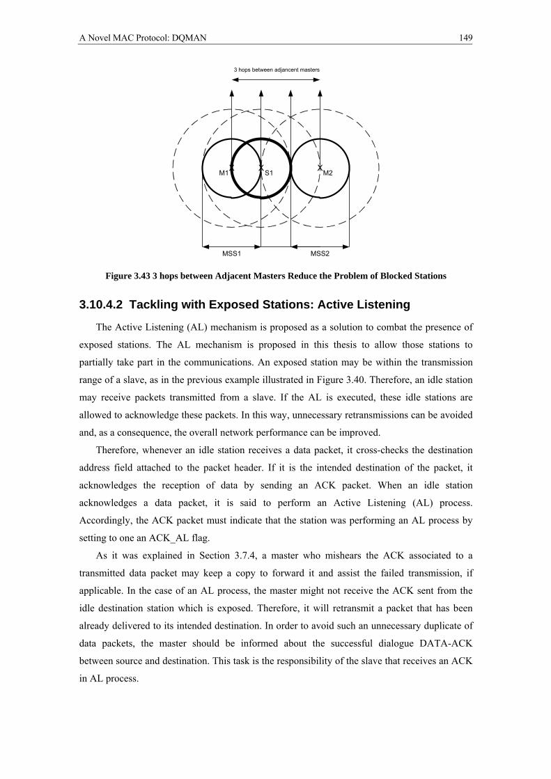
A Novel MAC Protocol: DQMAN
149
X X X
MSS2MSS1
M1 M2S1
3 hops between adjancent masters
Figure 3.43 3 hops between Adjacent Masters Reduce the Problem of Blocked Stations
3.10.4.2 Tackling with Exposed Stations: Active Listening
The Active Listening (AL) mechanism is proposed as a solution to combat the presence of
exposed stations. The AL mechanism is proposed in this thesis to allow those stations to
partially take part in the communications. An exposed station may be within the transmission
range of a slave, as in the previous example illustrated in Figure 3.40. Therefore, an idle station
may receive packets transmitted from a slave. If the AL is executed, these idle stations are
allowed to acknowledge these packets. In this way, unnecessary retransmissions can be avoided
and, as a consequence, the overall network performance can be improved.
Therefore, whenever an idle station receives a data packet, it cross-checks the destination
address field attached to the packet header. If it is the intended destination of the packet, it
acknowledges the reception of data by sending an ACK packet. When an idle station
acknowledges a data packet, it is said to perform an Active Listening (AL) process.
Accordingly, the ACK packet must indicate that the station was performing an AL process by
setting to one an ACK_AL flag.
As it was explained in Section 3.7.4, a master who mishears the ACK associated to a
transmitted data packet may keep a copy to forward it and assist the failed transmission, if
applicable. In the case of an AL process, the master might not receive the ACK sent from the
idle destination station which is exposed. Therefore, it will retransmit a packet that has been
already delivered to its intended destination. In order to avoid such an unnecessary duplicate of
data packets, the master should be informed about the successful dialogue DATA-ACK
between source and destination. This task is the responsibility of the slave that receives an ACK
in AL process.
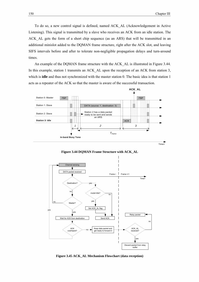
Chapter III
150
To do so, a new control signal is defined, named ACK_AL (Acknowledgement in Active
Listening). This signal is transmitted by a slave who receives an ACK from an idle station. The
ACK_AL gets the form of a short chip sequence (as an ARS) that will be transmitted in an
additional minislot added to the DQMAN frame structure, right after the ACK slot, and leaving
SIFS intervals before and after to tolerate non-negligible propagation delays and turn-around
times.
An example of the DQMAN frame structure with the ACK_AL is illustrated in Figure 3.44.
In this example, station 1 transmits an ACK_AL upon the reception of an ACK from station 3,
which is idle and thus not synchronized with the master station 0. The basic idea is that station 1
acts as a repeater of the ACK so that the master is aware of the successful transaction.
Tframe
Time+
In-band Busy Tone
Station 0: Master
Station 1: Slave
Station 3: Idle
FBP
ACK
DATA (source: 1, destination: 3)
FBP
Station 2: SlaveStation 2 has a data packet ready to be sent and sends
an ARS
1 2 3
ACK_AL
Figure 3.44 DQMAN Frame Structure with ACK_AL
no
yes
no
Frame i Frame i+1
Time+
Wait for ACK from destination
DATA packet received
Destination?
Send ACK
ACK overheard?
Keep data packet and get ready to forward it
Relay packet
ACK_AL received?
Discard packet from relay buffer
no
Master?
yes
Channel sensing
no
mode=Idle?
Set ACK_AL flag
no
yes
yes
yes
Figure 3.45 ACK_AL Mechanism Flowchart (data reception)
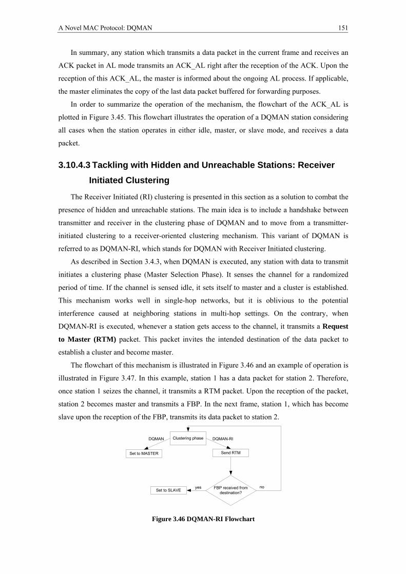
A Novel MAC Protocol: DQMAN
151
In summary, any station which transmits a data packet in the current frame and receives an
ACK packet in AL mode transmits an ACK_AL right after the reception of the ACK. Upon the
reception of this ACK_AL, the master is informed about the ongoing AL process. If applicable,
the master eliminates the copy of the last data packet buffered for forwarding purposes.
In order to summarize the operation of the mechanism, the flowchart of the ACK_AL is
plotted in Figure 3.45. This flowchart illustrates the operation of a DQMAN station considering
all cases when the station operates in either idle, master, or slave mode, and receives a data
packet.
3.10.4.3 Tackling with Hidden and Unreachable Stations: Receiver
Initiated Clustering
The Receiver Initiated (RI) clustering is presented in this section as a solution to combat the
presence of hidden and unreachable stations. The main idea is to include a handshake between
transmitter and receiver in the clustering phase of DQMAN and to move from a transmitter-
initiated clustering to a receiver-oriented clustering mechanism. This variant of DQMAN is
referred to as DQMAN-RI, which stands for DQMAN with Receiver Initiated clustering.
As described in Section 3.4.3, when DQMAN is executed, any station with data to transmit
initiates a clustering phase (Master Selection Phase). It senses the channel for a randomized
period of time. If the channel is sensed idle, it sets itself to master and a cluster is established.
This mechanism works well in single-hop networks, but it is oblivious to the potential
interference caused at neighboring stations in multi-hop settings. On the contrary, when
DQMAN-RI is executed, whenever a station gets access to the channel, it transmits a Request
to Master (RTM) packet. This packet invites the intended destination of the data packet to
establish a cluster and become master.
The flowchart of this mechanism is illustrated in Figure 3.46 and an example of operation is
illustrated in Figure 3.47. In this example, station 1 has a data packet for station 2. Therefore,
once station 1 seizes the channel, it transmits a RTM packet. Upon the reception of the packet,
station 2 becomes master and transmits a FBP. In the next frame, station 1, which has become
slave upon the reception of the FBP, transmits its data packet to station 2.
Send RTM
Clustering phase
Set to MASTER
FBP received from destination?
noSet to SLAVE
yes
DQMAN DQMAN-RI
Figure 3.46 DQMAN-RI Flowchart
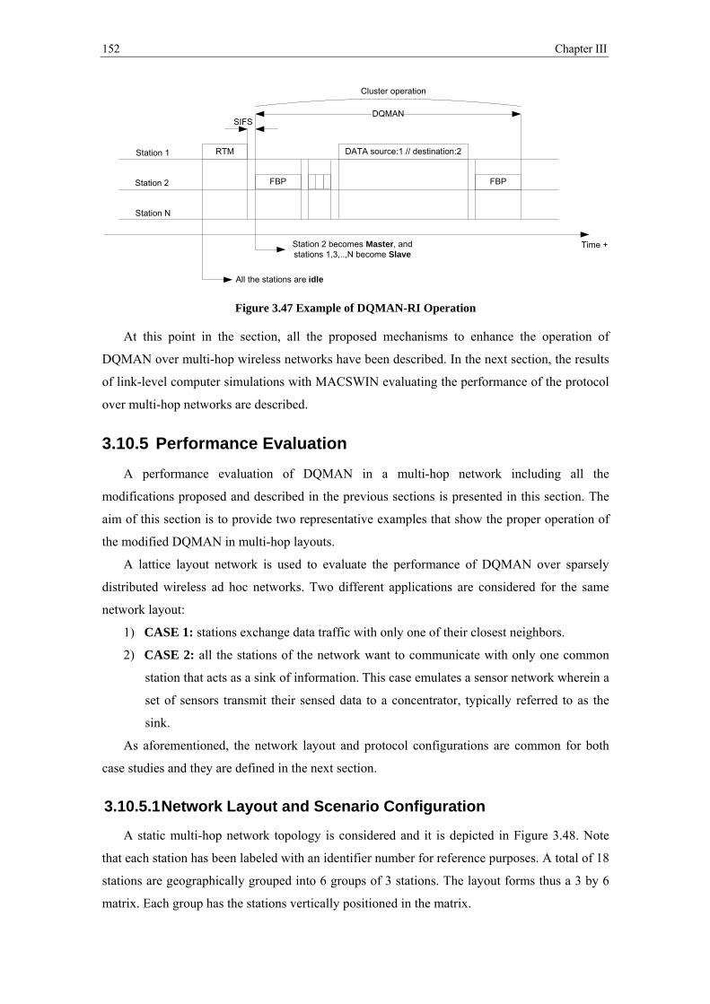
Chapter III
152
RTM
FBP
Station 1
Cluster operation
DQMAN
FBPStation 2
SIFS
DATA source:1 // destination:2
Station N
Time +Station 2 becomes Master, and stations 1,3,..,N become Slave
All the stations are idle
Figure 3.47 Example of DQMAN-RI Operation
At this point in the section, all the proposed mechanisms to enhance the operation of
DQMAN over multi-hop wireless networks have been described. In the next section, the results
of link-level computer simulations with MACSWIN evaluating the performance of the protocol
over multi-hop networks are described.
3.10.5 Performance Evaluation
A performance evaluation of DQMAN in a multi-hop network including all the
modifications proposed and described in the previous sections is presented in this section. The
aim of this section is to provide two representative examples that show the proper operation of
the modified DQMAN in multi-hop layouts.
A lattice layout network is used to evaluate the performance of DQMAN over sparsely
distributed wireless ad hoc networks. Two different applications are considered for the same
network layout:
1) CASE 1: stations exchange data traffic with only one of their closest neighbors.
2) CASE 2: all the stations of the network want to communicate with only one common
station that acts as a sink of information. This case emulates a sensor network wherein a
set of sensors transmit their sensed data to a concentrator, typically referred to as the
sink.
As aforementioned, the network layout and protocol configurations are common for both
case studies and they are defined in the next section.
3.10.5.1 Network Layout and Scenario Configuration
A static multi-hop network topology is considered and it is depicted in Figure 3.48. Note
that each station has been labeled with an identifier number for reference purposes. A total of 18
stations are geographically grouped into 6 groups of 3 stations. The layout forms thus a 3 by 6
matrix. Each group has the stations vertically positioned in the matrix.
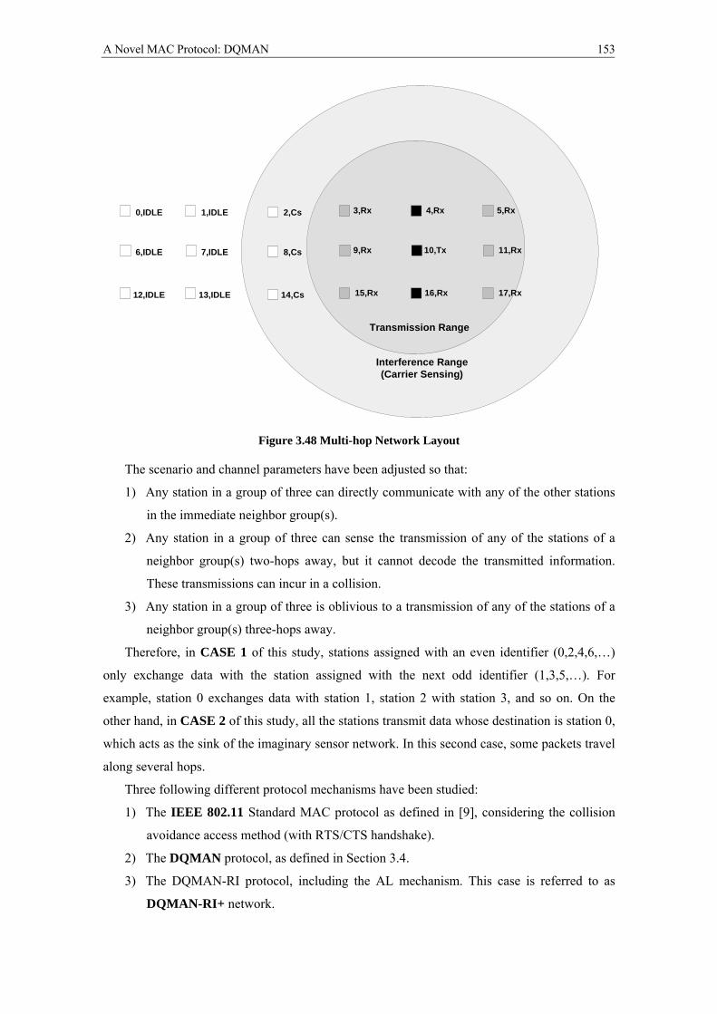
A Novel MAC Protocol: DQMAN
153
7,IDLE
Transmission Range
Interference Range(Carrier Sensing)
9,Rx 10,Tx8,Cs6,IDLE
13,IDLE 15,Rx 16,Rx14,Cs12,IDLE
1,IDLE 3,Rx 4,Rx2,Cs0,IDLE
11,Rx
17,Rx
5,Rx
Figure 3.48 Multi-hop Network Layout
The scenario and channel parameters have been adjusted so that:
1) Any station in a group of three can directly communicate with any of the other stations
in the immediate neighbor group(s).
2) Any station in a group of three can sense the transmission of any of the stations of a
neighbor group(s) two-hops away, but it cannot decode the transmitted information.
These transmissions can incur in a collision.
3) Any station in a group of three is oblivious to a transmission of any of the stations of a
neighbor group(s) three-hops away.
Therefore, in CASE 1 of this study, stations assigned with an even identifier (0,2,4,6,…)
only exchange data with the station assigned with the next odd identifier (1,3,5,…). For
example, station 0 exchanges data with station 1, station 2 with station 3, and so on. On the
other hand, in CASE 2 of this study, all the stations transmit data whose destination is station 0,
which acts as the sink of the imaginary sensor network. In this second case, some packets travel
along several hops.
Three following different protocol mechanisms have been studied:
1) The IEEE 802.11 Standard MAC protocol as defined in [9], considering the collision
avoidance access method (with RTS/CTS handshake).
2) The DQMAN protocol, as defined in Section 3.4.
3) The DQMAN-RI protocol, including the AL mechanism. This case is referred to as
DQMAN-RI+ network.
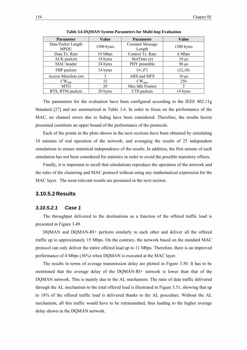
Chapter III
154
Table 3.6 DQMAN System Parameters for Multi-hop Evaluation
Parameter Value Parameter Value Data Packet Length
MPDU 1500 bytes
Constant Message Length
1500 bytes
Data Tx. Rate 54 Mbps Control Tx. Rate 6 Mbps ACK packets 14 bytes SlotTime (σ) 10 μs MAC header 34 bytes PHY preamble 96 μs
FBP packets 14 bytes , (32,10)
Access Minislots (m) 3 ARS and SIFS 10 μs CWmin 32 CWmax 256 MTO 20 Max Idle Frames 2
RTS, RTM packets 20 bytes CTS packets 14 bytes
The parameters for the evaluation have been configured according to the IEEE 802.11g
Standard [27] and are summarized in Table 3.6. In order to focus on the performance of the
MAC, no channel errors due to fading have been considered. Therefore, the results herein
presented constitute an upper bound of the performance of the protocols.
Each of the points in the plots shown in the next sections have been obtained by simulating
10 minutes of real operation of the network, and averaging the results of 25 independent
simulations to ensure statistical independence of the results. In addition, the first minute of each
simulation has not been considered for statistics in order to avoid the possible transitory effects.
Finally, it is important to recall that simulations reproduce the operation of the network and
the rules of the clustering and MAC protocol without using any mathematical expression for the
MAC layer. The most relevant results are presented in the next section.
3.10.5.2 Results
3.10.5.2.1 Case 1
The throughput delivered to the destinations as a function of the offered traffic load is
presented in Figure 3.49.
DQMAN and DQMAN-RI+ perform similarly to each other and deliver all the offered
traffic up to approximately 15 Mbps. On the contrary, the network based on the standard MAC
protocol can only deliver the entire offered load up to 11 Mbps. Therefore, there is an improved
performance of 4 Mbps (36%) when DQMAN is executed at the MAC layer.
The results in terms of average transmission delay are plotted in Figure 3.50. It has to be
mentioned that the average delay of the DQMAN-RI+ network is lower than that of the
DQMAN network. This is mainly due to the AL mechanism. The ratio of data traffic delivered
through the AL mechanism to the total offered load is illustrated in Figure 3.51, showing that up
to 18% of the offered traffic load is delivered thanks to the AL procedure. Without the AL
mechanism, all this traffic would have to be retransmitted, thus leading to the higher average
delay shown in the DQMAN network.
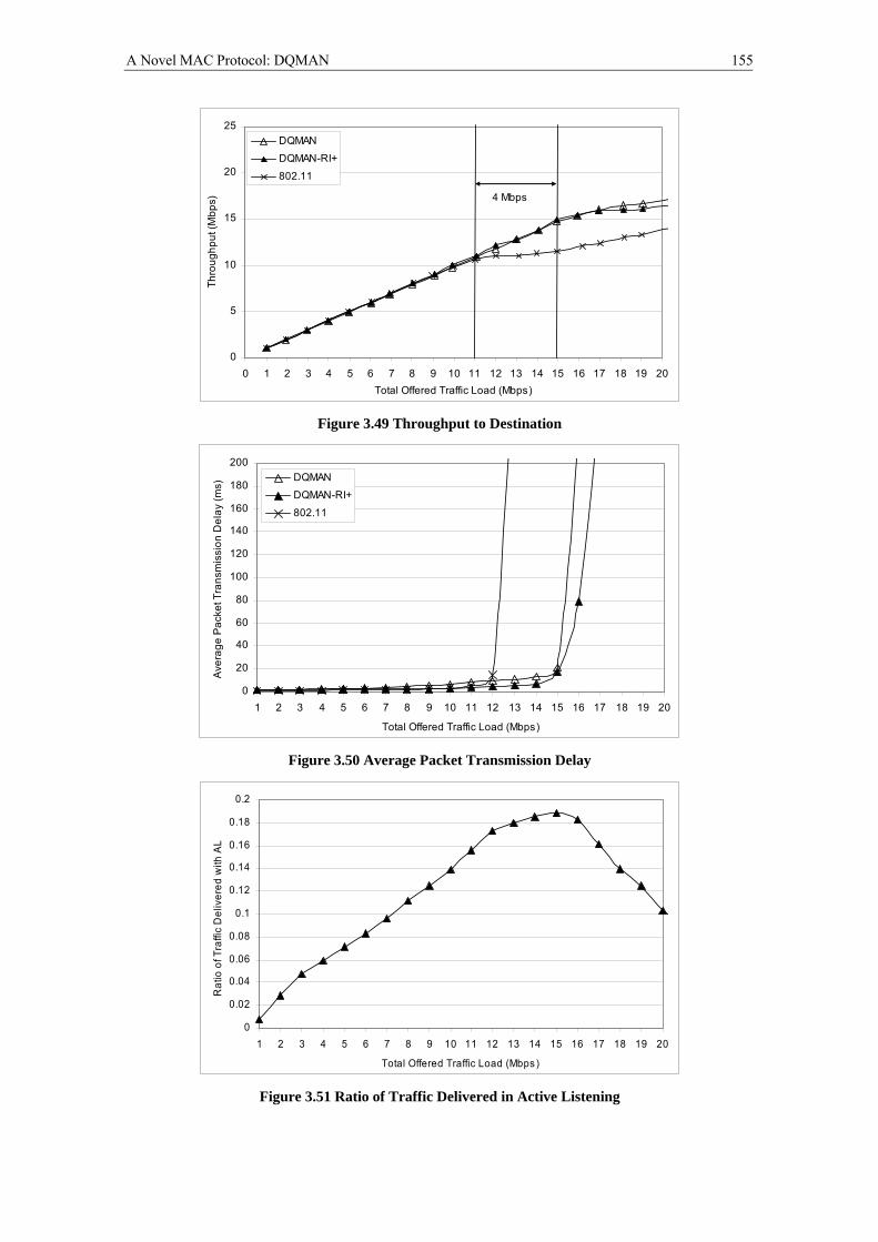
A Novel MAC Protocol: DQMAN
155
0
5
10
15
20
25
0 1 2 3 4 5 6 7 8 9 10 11 12 13 14 15 16 17 18 19 20
Total Offered Traffic Load (Mbps)
Th
rou
gh
pu
t (M
bp
s)
DQMAN
DQMAN-RI+
802.11
4 Mbps
Figure 3.49 Throughput to Destination
0
20
40
60
80
100
120
140
160
180
200
1 2 3 4 5 6 7 8 9 10 11 12 13 14 15 16 17 18 19 20
Total Offered Traffic Load (Mbps)
Ave
rag
e P
ack
et T
ran
smis
sio
n D
ela
y (m
s)
DQMAN
DQMAN-RI+
802.11
Figure 3.50 Average Packet Transmission Delay
0
0.02
0.04
0.06
0.08
0.1
0.12
0.14
0.16
0.18
0.2
1 2 3 4 5 6 7 8 9 10 11 12 13 14 15 16 17 18 19 20
Total Offered Traffic Load (Mbps)
Ra
tio o
f Tra
ffic
De
live
red
with
AL
Figure 3.51 Ratio of Traffic Delivered in Active Listening
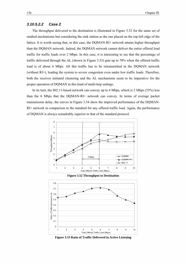
Chapter III
156
3.10.5.2.2 Case 2
The throughput delivered to the destination is illustrated in Figure 3.52 for the same set of
studied mechanisms but considering the sink station as the one placed on the top-left edge of the
lattice. It is worth seeing that, in this case, the DQMAN-RI+ network attains higher throughput
than the DQMAN network. Indeed, the DQMAN network cannot deliver the entire offered load
traffic for traffic loads over 2 Mbps. In this case, it is interesting to see that the percentage of
traffic delivered through the AL (shown in Figure 3.53) gets up to 70% when the offered traffic
load is of about 6 Mbps. All this traffic has to be retransmitted in the DQMAN network
(without RI+), leading the system to severe congestion even under low traffic loads. Therefore,
both the receiver initiated clustering and the AL mechanisms seem to be imperative for the
proper operation of DQMAN in this kind of multi-hop settings.
In its turn, the 802.11-based network can convey up to 4 Mbps, which is 2 Mbps (33%) less
than the 6 Mbps that the DQMAN-RI+ network can convey. In terms of average packet
transmission delay, the curves in Figure 3.54 show the improved performance of the DQMAN-
RI+ network in comparison to the standard for any offered traffic load. Again, the performance
of DQMAN is always remarkably superior to that of the standard protocol.
0
1
2
3
4
5
6
7
8
1 2 3 4 5 6 7 8 9 10
Total Offered Traffic Load (Mbps)
Th
rou
gh
pu
t (M
bp
s)
DQMAN
DQMAN-RI+
802.11
2 Mbps
Figure 3.52 Throughput to Destination
0
0.1
0.2
0.3
0.4
0.5
0.6
0.7
0.8
1 2 3 4 5 6 7 8 9 10
Total Offered Traffic Load (Mbps)
Ra
tio o
f Tra
ffic
De
live
red
in A
L
Figure 3.53 Ratio of Traffic Delivered in Active Listening
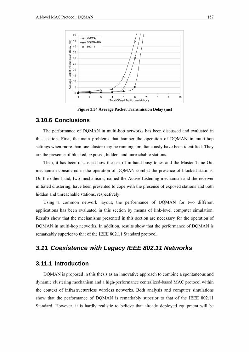
A Novel MAC Protocol: DQMAN
157
0
5
10
15
20
25
30
35
40
45
50
1 2 3 4 5 6 7 8 9 10Total Offered Traffic Load (Mbps)
Ave
rag
e P
ack
et T
ran
smis
sio
n D
ela
y (m
s)
DQMAN
DQMAN-RI+
802.11
Figure 3.54 Average Packet Transmission Delay (ms)
3.10.6 Conclusions
The performance of DQMAN in multi-hop networks has been discussed and evaluated in
this section. First, the main problems that hamper the operation of DQMAN in multi-hop
settings when more than one cluster may be running simultaneously have been identified. They
are the presence of blocked, exposed, hidden, and unreachable stations.
Then, it has been discussed how the use of in-band busy tones and the Master Time Out
mechanism considered in the operation of DQMAN combat the presence of blocked stations.
On the other hand, two mechanisms, named the Active Listening mechanism and the receiver
initiated clustering, have been presented to cope with the presence of exposed stations and both
hidden and unreachable stations, respectively.
Using a common network layout, the performance of DQMAN for two different
applications has been evaluated in this section by means of link-level computer simulation.
Results show that the mechanisms presented in this section are necessary for the operation of
DQMAN in multi-hop networks. In addition, results show that the performance of DQMAN is
remarkably superior to that of the IEEE 802.11 Standard protocol.
3.11 Coexistence with Legacy IEEE 802.11 Networks
3.11.1 Introduction
DQMAN is proposed in this thesis as an innovative approach to combine a spontaneous and
dynamic clustering mechanism and a high-performance centralized-based MAC protocol within
the context of infrastructureless wireless networks. Both analysis and computer simulations
show that the performance of DQMAN is remarkably superior to that of the IEEE 802.11
Standard. However, it is hardly realistic to believe that already deployed equipment will be
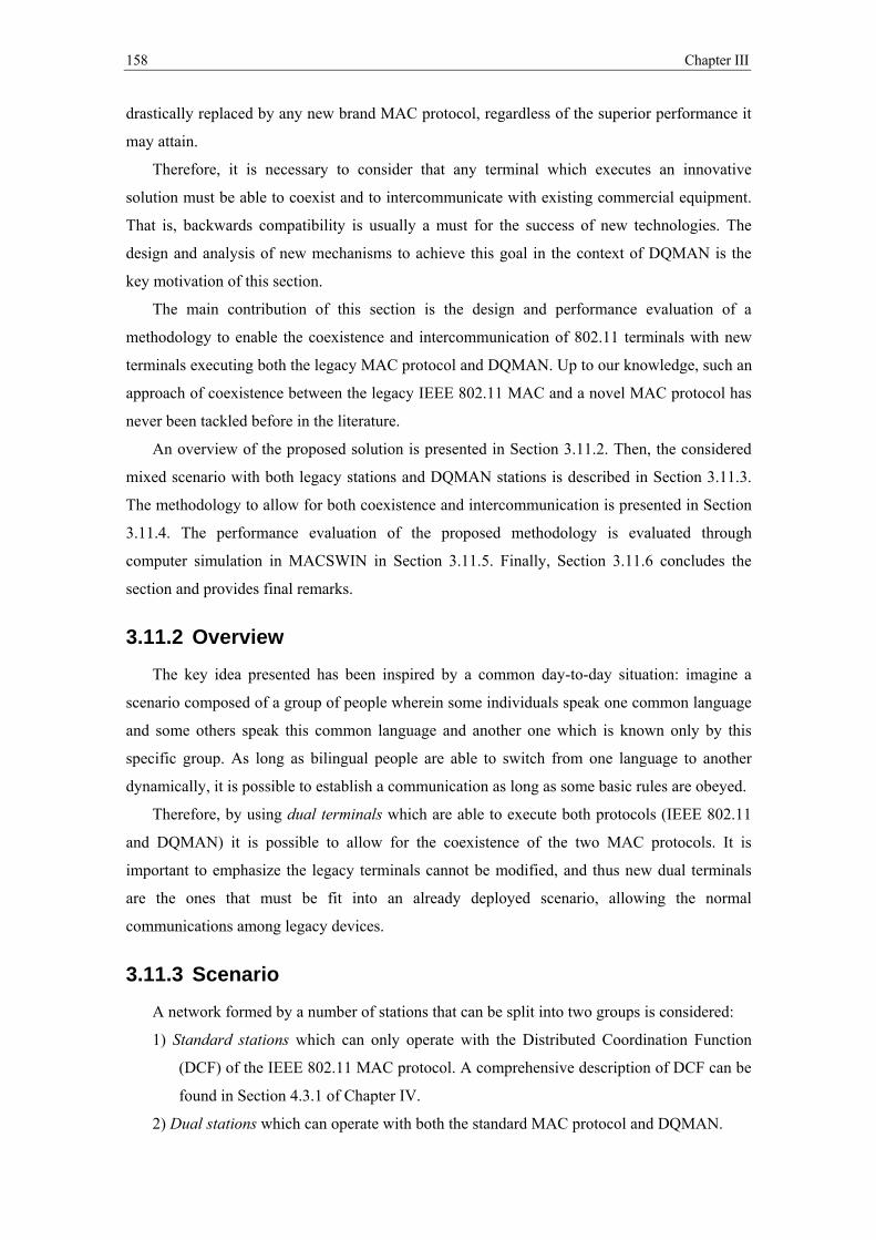
Chapter III
158
drastically replaced by any new brand MAC protocol, regardless of the superior performance it
may attain.
Therefore, it is necessary to consider that any terminal which executes an innovative
solution must be able to coexist and to intercommunicate with existing commercial equipment.
That is, backwards compatibility is usually a must for the success of new technologies. The
design and analysis of new mechanisms to achieve this goal in the context of DQMAN is the
key motivation of this section.
The main contribution of this section is the design and performance evaluation of a
methodology to enable the coexistence and intercommunication of 802.11 terminals with new
terminals executing both the legacy MAC protocol and DQMAN. Up to our knowledge, such an
approach of coexistence between the legacy IEEE 802.11 MAC and a novel MAC protocol has
never been tackled before in the literature.
An overview of the proposed solution is presented in Section 3.11.2. Then, the considered
mixed scenario with both legacy stations and DQMAN stations is described in Section 3.11.3.
The methodology to allow for both coexistence and intercommunication is presented in Section
3.11.4. The performance evaluation of the proposed methodology is evaluated through
computer simulation in MACSWIN in Section 3.11.5. Finally, Section 3.11.6 concludes the
section and provides final remarks.
3.11.2 Overview
The key idea presented has been inspired by a common day-to-day situation: imagine a
scenario composed of a group of people wherein some individuals speak one common language
and some others speak this common language and another one which is known only by this
specific group. As long as bilingual people are able to switch from one language to another
dynamically, it is possible to establish a communication as long as some basic rules are obeyed.
Therefore, by using dual terminals which are able to execute both protocols (IEEE 802.11
and DQMAN) it is possible to allow for the coexistence of the two MAC protocols. It is
important to emphasize the legacy terminals cannot be modified, and thus new dual terminals
are the ones that must be fit into an already deployed scenario, allowing the normal
communications among legacy devices.
3.11.3 Scenario
A network formed by a number of stations that can be split into two groups is considered:
1) Standard stations which can only operate with the Distributed Coordination Function
(DCF) of the IEEE 802.11 MAC protocol. A comprehensive description of DCF can be
found in Section 4.3.1 of Chapter IV.
2) Dual stations which can operate with both the standard MAC protocol and DQMAN.
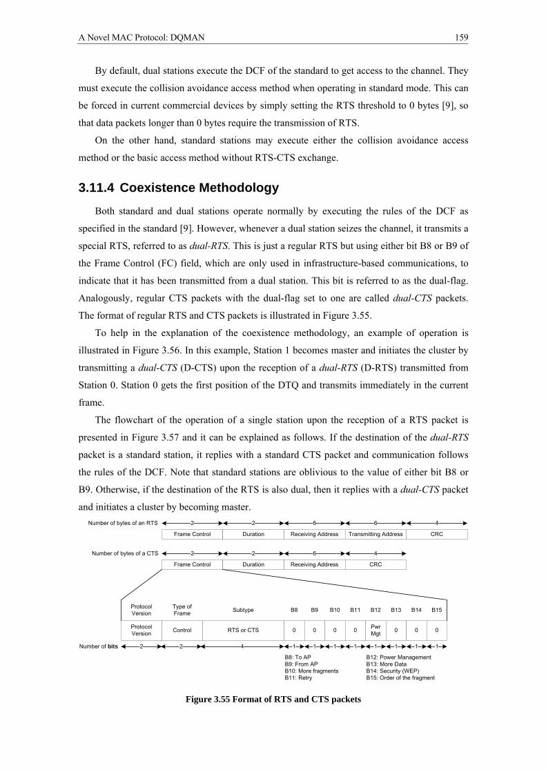
A Novel MAC Protocol: DQMAN
159
By default, dual stations execute the DCF of the standard to get access to the channel. They
must execute the collision avoidance access method when operating in standard mode. This can
be forced in current commercial devices by simply setting the RTS threshold to 0 bytes [9], so
that data packets longer than 0 bytes require the transmission of RTS.
On the other hand, standard stations may execute either the collision avoidance access
method or the basic access method without RTS-CTS exchange.
3.11.4 Coexistence Methodology
Both standard and dual stations operate normally by executing the rules of the DCF as
specified in the standard [9]. However, whenever a dual station seizes the channel, it transmits a
special RTS, referred to as dual-RTS. This is just a regular RTS but using either bit B8 or B9 of
the Frame Control (FC) field, which are only used in infrastructure-based communications, to
indicate that it has been transmitted from a dual station. This bit is referred to as the dual-flag.
Analogously, regular CTS packets with the dual-flag set to one are called dual-CTS packets.
The format of regular RTS and CTS packets is illustrated in Figure 3.55.
To help in the explanation of the coexistence methodology, an example of operation is
illustrated in Figure 3.56. In this example, Station 1 becomes master and initiates the cluster by
transmitting a dual-CTS (D-CTS) upon the reception of a dual-RTS (D-RTS) transmitted from
Station 0. Station 0 gets the first position of the DTQ and transmits immediately in the current
frame.
The flowchart of the operation of a single station upon the reception of a RTS packet is
presented in Figure 3.57 and it can be explained as follows. If the destination of the dual-RTS
packet is a standard station, it replies with a standard CTS packet and communication follows
the rules of the DCF. Note that standard stations are oblivious to the value of either bit B8 or
B9. Otherwise, if the destination of the RTS is also dual, then it replies with a dual-CTS packet
and initiates a cluster by becoming master.
Protocol Version
Control RTS or CTS 0 0 0 0Pwr Mgt
0 0 0
2 2 4 1 1 1 1 1 1 1 1Number of bits
Frame Control Duration Receiving Address CRC
2 2 6 4Number of bytes of a CTS
Protocol Version
Type of Frame
Subtype B8 B9 B10 B11 B12 B13 B14 B15
B8: To APB9: From APB10: More fragmentsB11: Retry
B12: Power ManagementB13: More DataB14: Security (WEP)B15: Order of the fragment
Frame Control Duration Receiving Address CRC
2 2 6 4
Transmitting Address
6Number of bytes of an RTS
Figure 3.55 Format of RTS and CTS packets
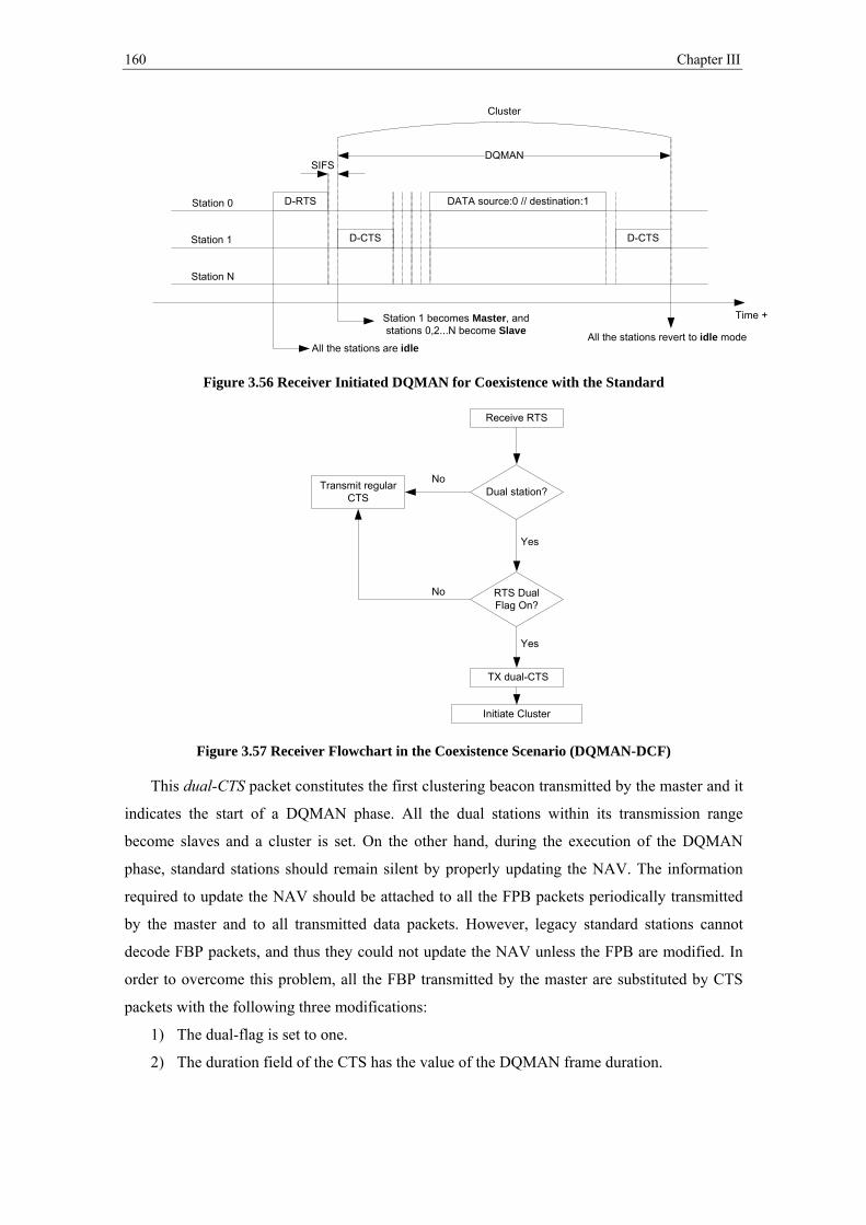
Chapter III
160
D-RTS
D-CTS
Station 0
Cluster
DQMAN
D-CTSStation 1
SIFS
DATA source:0 // destination:1
Station N
Time +Station 1 becomes Master, and stations 0,2...N become Slave
All the stations revert to idle modeAll the stations are idle
Figure 3.56 Receiver Initiated DQMAN for Coexistence with the Standard
Receive RTS
Dual station?
RTS Dual Flag On?
Transmit regular CTS
TX dual-CTS
No
Yes
No
Yes
Initiate Cluster
Figure 3.57 Receiver Flowchart in the Coexistence Scenario (DQMAN-DCF)
This dual-CTS packet constitutes the first clustering beacon transmitted by the master and it
indicates the start of a DQMAN phase. All the dual stations within its transmission range
become slaves and a cluster is set. On the other hand, during the execution of the DQMAN
phase, standard stations should remain silent by properly updating the NAV. The information
required to update the NAV should be attached to all the FPB packets periodically transmitted
by the master and to all transmitted data packets. However, legacy standard stations cannot
decode FBP packets, and thus they could not update the NAV unless the FPB are modified. In
order to overcome this problem, all the FBP transmitted by the master are substituted by CTS
packets with the following three modifications:
1) The dual-flag is set to one.
2) The duration field of the CTS has the value of the DQMAN frame duration.
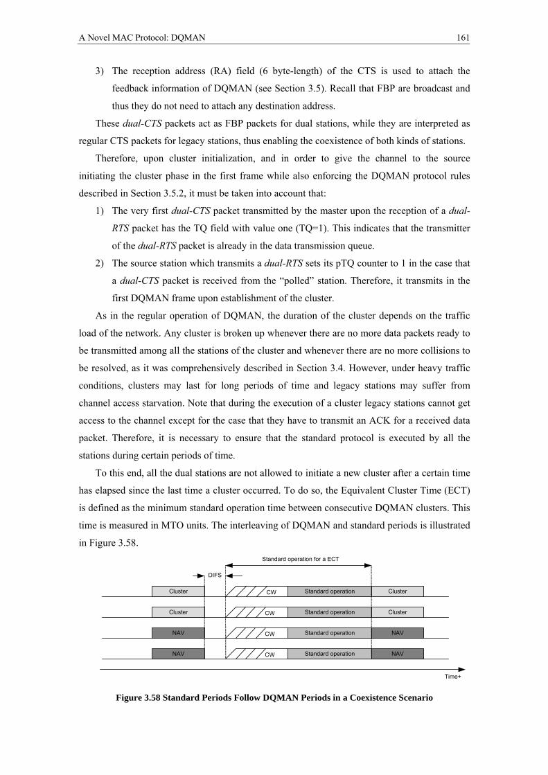
A Novel MAC Protocol: DQMAN
161
3) The reception address (RA) field (6 byte-length) of the CTS is used to attach the
feedback information of DQMAN (see Section 3.5). Recall that FBP are broadcast and
thus they do not need to attach any destination address.
These dual-CTS packets act as FBP packets for dual stations, while they are interpreted as
regular CTS packets for legacy stations, thus enabling the coexistence of both kinds of stations.
Therefore, upon cluster initialization, and in order to give the channel to the source
initiating the cluster phase in the first frame while also enforcing the DQMAN protocol rules
described in Section 3.5.2, it must be taken into account that:
1) The very first dual-CTS packet transmitted by the master upon the reception of a dual-
RTS packet has the TQ field with value one (TQ=1). This indicates that the transmitter
of the dual-RTS packet is already in the data transmission queue.
2) The source station which transmits a dual-RTS sets its pTQ counter to 1 in the case that
a dual-CTS packet is received from the “polled” station. Therefore, it transmits in the
first DQMAN frame upon establishment of the cluster.
As in the regular operation of DQMAN, the duration of the cluster depends on the traffic
load of the network. Any cluster is broken up whenever there are no more data packets ready to
be transmitted among all the stations of the cluster and whenever there are no more collisions to
be resolved, as it was comprehensively described in Section 3.4. However, under heavy traffic
conditions, clusters may last for long periods of time and legacy stations may suffer from
channel access starvation. Note that during the execution of a cluster legacy stations cannot get
access to the channel except for the case that they have to transmit an ACK for a received data
packet. Therefore, it is necessary to ensure that the standard protocol is executed by all the
stations during certain periods of time.
To this end, all the dual stations are not allowed to initiate a new cluster after a certain time
has elapsed since the last time a cluster occurred. To do so, the Equivalent Cluster Time (ECT)
is defined as the minimum standard operation time between consecutive DQMAN clusters. This
time is measured in MTO units. The interleaving of DQMAN and standard periods is illustrated
in Figure 3.58.
Cluster
Cluster
NAV
DIFS
Standard operation for a ECT
CW
CW
CW Standard operation
Standard operation
Standard operation
Cluster
Cluster
NAV
Time+
NAV CW Standard operation NAV
Figure 3.58 Standard Periods Follow DQMAN Periods in a Coexistence Scenario
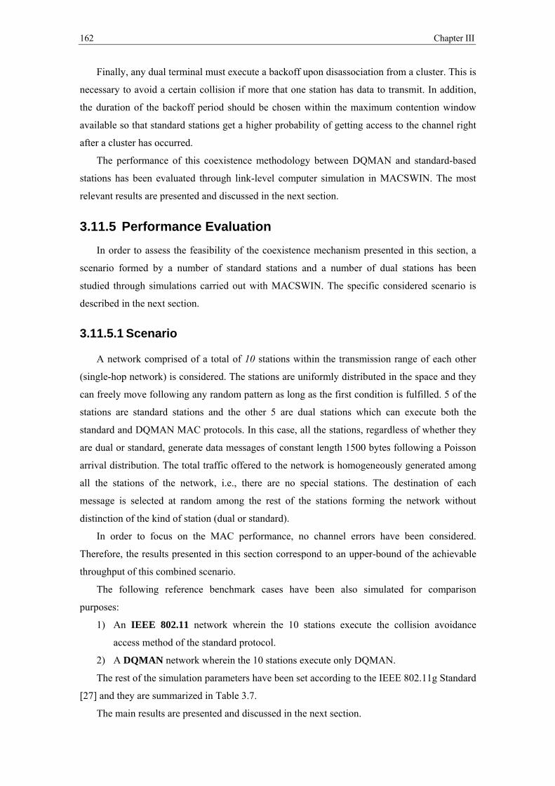
Chapter III
162
Finally, any dual terminal must execute a backoff upon disassociation from a cluster. This is
necessary to avoid a certain collision if more that one station has data to transmit. In addition,
the duration of the backoff period should be chosen within the maximum contention window
available so that standard stations get a higher probability of getting access to the channel right
after a cluster has occurred.
The performance of this coexistence methodology between DQMAN and standard-based
stations has been evaluated through link-level computer simulation in MACSWIN. The most
relevant results are presented and discussed in the next section.
3.11.5 Performance Evaluation
In order to assess the feasibility of the coexistence mechanism presented in this section, a
scenario formed by a number of standard stations and a number of dual stations has been
studied through simulations carried out with MACSWIN. The specific considered scenario is
described in the next section.
3.11.5.1 Scenario
A network comprised of a total of 10 stations within the transmission range of each other
(single-hop network) is considered. The stations are uniformly distributed in the space and they
can freely move following any random pattern as long as the first condition is fulfilled. 5 of the
stations are standard stations and the other 5 are dual stations which can execute both the
standard and DQMAN MAC protocols. In this case, all the stations, regardless of whether they
are dual or standard, generate data messages of constant length 1500 bytes following a Poisson
arrival distribution. The total traffic offered to the network is homogeneously generated among
all the stations of the network, i.e., there are no special stations. The destination of each
message is selected at random among the rest of the stations forming the network without
distinction of the kind of station (dual or standard).
In order to focus on the MAC performance, no channel errors have been considered.
Therefore, the results presented in this section correspond to an upper-bound of the achievable
throughput of this combined scenario.
The following reference benchmark cases have been also simulated for comparison
purposes:
1) An IEEE 802.11 network wherein the 10 stations execute the collision avoidance
access method of the standard protocol.
2) A DQMAN network wherein the 10 stations execute only DQMAN.
The rest of the simulation parameters have been set according to the IEEE 802.11g Standard
[27] and they are summarized in Table 3.7.
The main results are presented and discussed in the next section.
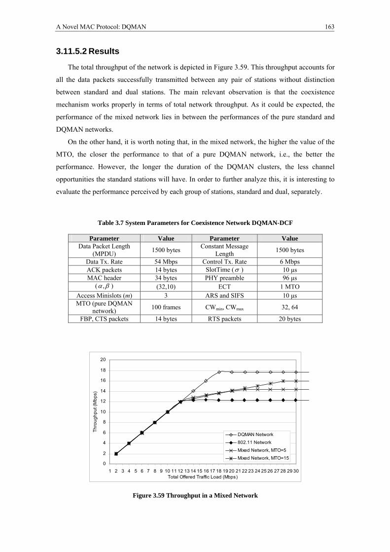
A Novel MAC Protocol: DQMAN
163
3.11.5.2 Results
The total throughput of the network is depicted in Figure 3.59. This throughput accounts for
all the data packets successfully transmitted between any pair of stations without distinction
between standard and dual stations. The main relevant observation is that the coexistence
mechanism works properly in terms of total network throughput. As it could be expected, the
performance of the mixed network lies in between the performances of the pure standard and
DQMAN networks.
On the other hand, it is worth noting that, in the mixed network, the higher the value of the
MTO, the closer the performance to that of a pure DQMAN network, i.e., the better the
performance. However, the longer the duration of the DQMAN clusters, the less channel
opportunities the standard stations will have. In order to further analyze this, it is interesting to
evaluate the performance perceived by each group of stations, standard and dual, separately.
Table 3.7 System Parameters for Coexistence Network DQMAN-DCF
Parameter Value Parameter Value Data Packet Length
(MPDU) 1500 bytes
Constant Message Length
1500 bytes
Data Tx. Rate 54 Mbps Control Tx. Rate 6 Mbps ACK packets 14 bytes SlotTime ( ) 10 μs MAC header 34 bytes PHY preamble 96 μs
( , ) (32,10) ECT 1 MTO Access Minislots (m) 3 ARS and SIFS 10 μs MTO (pure DQMAN
network) 100 frames CWmin, CWmax 32, 64
FBP, CTS packets 14 bytes RTS packets 20 bytes
0
2
4
6
8
10
12
14
16
18
20
1 2 3 4 5 6 7 8 9 10 11 12 13 14 15 16 17 18 19 20 21 22 23 24 25 26 27 28 29 30Total Offered Traffic Load (Mbps)
Th
rou
gh
pu
t (M
bp
s)
DQMAN Network
802.11 Network
Mixed Network, MTO=5
Mixed Network, MTO=15
Figure 3.59 Throughput in a Mixed Network
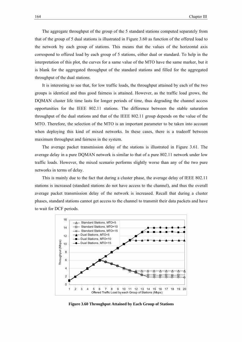
Chapter III
164
The aggregate throughput of the group of the 5 standard stations computed separately from
that of the group of 5 dual stations is illustrated in Figure 3.60 as function of the offered load to
the network by each group of stations. This means that the values of the horizontal axis
correspond to offered load by each group of 5 stations, either dual or standard. To help in the
interpretation of this plot, the curves for a same value of the MTO have the same marker, but it
is blank for the aggregated throughput of the standard stations and filled for the aggregated
throughput of the dual stations.
It is interesting to see that, for low traffic loads, the throughput attained by each of the two
groups is identical and thus good fairness is attained. However, as the traffic load grows, the
DQMAN cluster life time lasts for longer periods of time, thus degrading the channel access
opportunities for the IEEE 802.11 stations. The difference between the stable saturation
throughput of the dual stations and that of the IEEE 802.11 group depends on the value of the
MTO. Therefore, the selection of the MTO is an important parameter to be taken into account
when deploying this kind of mixed networks. In these cases, there is a tradeoff between
maximum throughput and fairness in the system.
The average packet transmission delay of the stations is illustrated in Figure 3.61. The
average delay in a pure DQMAN network is similar to that of a pure 802.11 network under low
traffic loads. However, the mixed scenario performs slightly worse than any of the two pure
networks in terms of delay.
This is mainly due to the fact that during a cluster phase, the average delay of IEEE 802.11
stations is increased (standard stations do not have access to the channel), and thus the overall
average packet transmission delay of the network is increased. Recall that during a cluster
phases, standard stations cannot get access to the channel to transmit their data packets and have
to wait for DCF periods.
0
2
4
6
8
10
12
14
16
1 2 3 4 5 6 7 8 9 10 11 12 13 14 15 16 17 18 19 20Offered Traffic Load by each Group of Stations (Mbps)
Th
rou
gh
pu
t (M
bp
s)
Standard Stations, MTO=5
Standard Stations, MTO=10
Standard Stations, MTO=15Dual Stations, MTO=5
Dual Stations, MTO=10
Dual Stations, MTO=15
Figure 3.60 Throughput Attained by Each Group of Stations
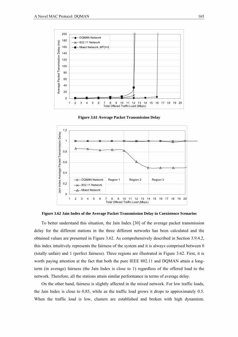
A Novel MAC Protocol: DQMAN
165
0
20
40
60
80
100
120
140
160
180
200
1 2 3 4 5 6 7 8 9 10 11 12 13 14 15 16 17 18 19 20Total Offered Traffic Load (Mbps)
Ave
rag
e P
ack
et T
ran
smis
sio
n D
ela
y (m
s)
DQMAN Network
802.11 Network
Mixed Network, MTO=5
Figure 3.61 Average Packet Transmission Delay
0
0,2
0,4
0,6
0,8
1
1,2
1 2 3 4 5 6 7 8 9 10 11 12 13 14 15 16 17 18 19 20Total Offered Traffic Load (Mbps)
Jain
Ind
ex
Ave
rag
e P
ack
et T
ran
smis
sio
n D
ela
y
DQMAN Network
802.11 Network
Mixed Network
Region 1 Region 2 Region 3
Figure 3.62 Jain Index of the Average Packet Transmission Delay in Coexistence Scenarios
To better understand this situation, the Jain Index [30] of the average packet transmission
delay for the different stations in the three different networks has been calculated and the
obtained values are presented in Figure 3.62. As comprehensively described in Section 3.9.4.2,
this index intuitively represents the fairness of the system and it is always comprised between 0
(totally unfair) and 1 (perfect fairness). Three regions are illustrated in Figure 3.62. First, it is
worth paying attention at the fact that both the pure IEEE 802.11 and DQMAN attain a long-
term (in average) fairness (the Jain Index is close to 1) regardless of the offered load to the
network. Therefore, all the stations attain similar performance in terms of average delay.
On the other hand, fairness is slightly affected in the mixed network. For low traffic loads,
the Jain Index is close to 0.85, while as the traffic load grows it drops to approximately 0.5.
When the traffic load is low, clusters are established and broken with high dynamism.
Chapter III
166
Therefore, all the stations of the network (standard and duals) get similar channel access
opportunities. The fact that the Jain Index is not equal to one is due to the fact that the average
packet transmission delay perceived by dual stations is lower when DQMAN is executed.
However, as the traffic load grows, the cluster life time increases. This has a negative impact on
standard stations, which get less channel access opportunities and thus a lower value of the Jain
Index close to 0.5 is attained. This value clearly represents that there are two separated groups
perceiving different average access delays, but the average access delay within each group is
very homogeneous.
3.11.6 Conclusions
The feasibility of the coexistence and intercommunication of the IEEE 802.11 Standard
MAC protocol with DQMAN has been assessed and evaluated in this section. This analysis is
very important in the light of the potential commercial exploitation of DQMAN. The results are
rather promising. As already discussed in the introduction of this section, it is unrealistic to
believe that any new technology will drastically substitute legacy one no matter the better
performance it can attain, and thus backwards compatibility is a must for the success of any new
technology.
The results presented in this section show that by using dual terminals capable of
interchangeably executing the two protocols it is possible to run a mixed network formed by
standard and dual terminals simultaneously and to attain good performance figures. It is
important to emphasize that communication can be performed between any pair of stations,
regardless of whether they are standard or dual. In this case, dual terminals have to take into
account the set of rules that drive the operation of standard stations in order to avoid severe
unfairness in the channel access. Therefore, standard-based periods must be guaranteed.
However, it has to be taken into account that long periods of DQMAN operation lead to
higher throughput, but also may yield channel access starvation for standard stations. This
tradeoff should be managed considering higher-layer requirements. In some applications it
might be necessary to attain maximum fairness among all the users of a network, while in other
applications it may be interesting to give priority to a set of users regardless of the impact on the
other users.
3.12 Chapter Conclusions
DQMAN has been presented in this chapter as an innovative concept design to extend the
high-performance of infrastructure-based MAC protocols to distributed networks without
infrastructure. The particular focus has been put on extending the near-optimum performance of
DQCA to infrastructureless networks. By embedding a layer-2 dynamic, passive, and
A Novel MAC Protocol: DQMAN
167
spontaneous clustering mechanism with a modified DQCA, it has been possible to extend the
outstanding performance of the latter to infrastructureless networks.
The main idea behind DQMAN is that any idle station gets access to the channel in a
similar way to the distributed channel access method of the IEEE 802.11 Standard (DCF).
However, once a station seizes the channel, it becomes the spontaneous clusterhead of a
temporary cluster. This station acts as an indirect coordinator for the peer-to-peer
communication links that can be established between the stations in the cluster, using the rules
based on DQCA. The duration of the cluster exclusively depends on the load of the network.
Whenever there are no more data packets to transmit, the cluster is broken.
DQMAN attains very high performance in single-hop networks by attaining a high stable
saturation throughput regardless of the number of users of the network. It operates as a random
access protocol for low traffic loads and it switches smoothly and automatically to a reservation
protocol as the traffic load grows. Collisions in the transmission of data packets are completely
avoided and contention is confined to a small portion of the resources and to clustering phases.
The performance of the network in this layout has been analytically modeled. Firstly, a model to
compute the saturation throughput of DQMAN has been presented. The model is based on
Markov chain theory and allows modeling the operation of the network in an accurate manner.
Then, the model has been extended to analyze the protocol under non-saturated conditions by
combining Markov chain modeling with classical queueing theory to model the operation of the
protocol within each cluster. In this latter case, the model also allows computing the average
message transmission delay as well as some other clustering metrics. Link-level computer
simulations with MACSWIN show that the model accurately matches the simulated
performance of the network under different scenarios.
Despite the high-performance of the protocol, further evaluation of the protocol operation
showed that there was yet room for more improvement under heavy traffic conditions. Two
simple mechanisms have been also presented to push the DQMAN performance to the
maximum capacity of the system over single-hop networks.
On the other hand, the performance of the DQMAN in multi-hop environments has been
also evaluated by computer simulation. Rather than presenting a comprehensive evaluation of
the protocol under any multi-hop scenario, two representative cases have been presented to
show that the protocol can run over sparsely distributed networks. Any application would
require a specific evaluation and optimization of the protocol in order to get the best of it. In any
case, it has been shown that the inter-cluster interference may degrade the performance of the
protocol when not all the stations are in the transmission range of each other and more than one
station can operate in master mode simultaneously. In addition, it has been shown that the
CSMA-based clustering of DQMAN leads to some well known effects such as the presence of
hidden or exposed terminals that may hamper the performance of the protocol. To cope with
Chapter III
168
these problems, three mechanisms have been presented in this chapter. It has been shown that
the in-band busy tones of DQMAN effectively combat the presence of blocked stations. In
addition, a new mechanism has been also presented to solve the problem of stations exposed
and to improve the performance of the DQMAN in multi-hop networks. And finally, a new
version of DQMAN based on a receiver-oriented clustering has been presented. It has been
named DQMAN-RI, and, analogously with the two access methods of the IEEE 802.11
Standard, it constitutes the collision avoidance access method of DQMAN, suitable for
execution over multi-hop environments.
Despite the high-performance of DQMAN over both single-hop and multi-hop
environments, it is hardly realistic to believe that any new technology would replace current
equipment no matter the good performance it can attain. Therefore, backwards compatibility is
always a must for the successful penetration of new technology in the market. For this reason,
the last part of this chapter has been devoted to the design and evaluation of a mechanism that
allows the coexistence and intercommunication between DQMAN legacy IEEE 802.11
standard-based equipment. Computer simulations show that DQMAN and the IEEE 802.11
MAC protocol can successfully coexist and intercommunicate.
The ideas presented in this chapter can indeed be used to extend the execution of any other
infrastructure-based MAC protocol to distributed infrastructureless networks. In order to
exemplify this, the next chapter of the thesis is devoted to present, in a brief manner, the design
of the Distributed Point Coordination Function (DPCF). This protocol constitutes the extension
of the Point Coordination Function of the 802.11 Standard, conceived to provide QoS in
centralized networks, to infrastructureless networks. The methodology to design the protocol is
completely based on DQMAN and constitutes an example of how the ideas presented in this
chapter can be applied to any other MAC protocol.
3.13 References
[1] L. Kleinrock and F. A. Tobagi, “Packet Switching in radio channels: Part I – Carrier
Sense Multiple-Access Models and their Throughput-Delay Characteristics,” IEEE
Trans. on Comm., vol. 23, pp. 1400-1416, Dec. 1975.
[2] J. Alonso-Zárate, E. Kartsakli, A. Cateura, C. Verikoukis, and L. Alonso, “A Near-
Optimum Cross-Layered Distributed Queueing Protocol for WLAN,” IEEE Wireless
Communications Magazine Special Issue on Medium Access Control Protocols for
Wireless LANs, vol. 15, no. 1, pp. 48-55, Feb. 2008.
[3] IEEE, Part 11: Wireless LAN Medium Access Control (MAC) and Physical Layer
(PHY) Specifications, IEEE Std. 802.-11-99, Aug. 1999.
[4] W. Xu and G. Campbell, “A Near Perfect Stable Random Access Protocol for a
Broadcast Channel,” in Proc. of the IEEE International Conference on Communications
A Novel MAC Protocol: DQMAN
169
1992 (ICC’92), vol. 1, pp. 370-374, 1992.
[5] C. T. Wu and G. Campbell, “Extended DQRAP (XDQRAP) A Cable TV Protocol
Functioning as a Distributed Switch,” in Proc. of the IEEE 1st International Workshop
on Community Networking Integrated Multimedia Services to The Home, pp. 191-198,
1994.
[6] H. J. Lin and G. Campbell, “PDQRAP – Prioritized Distributed Queueing Random
Access Protocol,” in Proc. of the IEEE Conference on Local Computer Networks,
Minneapolis, MN, USA, pp. 82-91, 1994.
[7] C. T. Wu and G. Campbell, “Interleaved DQRAP with Global TQ,” Internal Report,
Department of Computer Science, Illinois Institute of Technology, 1994.
[8] L. Alonso, R. Agustí, and O. Sallent, “A Near-Optimum MAC Protocol Based on the
Distributed Queueing Random Access Protocol (DQRAP) for a CDMA Mobile
Communication System,” IEEE Journal on Selected Areas in Communications, vol. 18,
no. 9, pp. 1701-1718, Sep. 2000.
[9] C. Prehofer and C. Bettstetter, “Self-Organization in Communication Networks:
Principles and Design Paradigms,” IEEE Communications Magazine, vol. 43, no. 7, pp.
78-85, Jul. 2005.
[10] J. Y. Yu and P. H. J. Chong, “A Survey of Clustering Schemes for Mobile Ad Hoc
Networks,” IEEE Communications Surveys & Tutorials, vol. 7, no. 1, pp. 32-48, First
Quarter 2005.
[11] D. Wei and H. A. Chan, “A Survey on Cluster Schemes in Ad Hoc Wireless Networks,”
IEE Mobility Conference, GuangZhou, 2005.
[12] C. Li, “Clustering in Packet Radio Networks,” in Proc. of the IEEE International
Conference on Communications (ICC’85).
[13] T. Kwon, M. Gerla, V. K. Varma, M. Barton, and T. R. Hsing, “Efficient flooding with
passive clustering – an overhead-free selective forward mechanism for ad hoc/sensor
networks,” in Proc. of the IEEE, vol. 91, no.8, pp. 1210-1220, Aug. 2003.
[14] J. Alonso, C. Verikoukis, and L. Alonso, “Fairness Enhancement in a Self-Configuring
Cluster-Based Wireless Ad Hoc Network,” in Proc. of the WPMC’05, Aalborg,
Denmark, Sep. 2005.
[15] Campbell et al. “Method and apparatus for detecting collisions and controlling access to
a communications channel,” US Patent no. US6408009 B1, Jun. 2002.
[16] E. Kartsakli, J. Alonso-Zárate, A. Cateura, Ch. Verikoukis, and L. Alonso, “Medium
Access Control in Wireless Networks,” published by Nova Science Publishers Inc,
ISBN-1-60021-944-6. Chapter 2, “Contention-Based Collision-Resolution Medium
Access Control Algorithms,” Feb. 2008.
[17] J. Yeo and A. Agrawala, “Packet Error Model for the IEEE 802.11 MAC Protocol,” in
Chapter III
170
Proc. of the IEEE PIMRC 2003, pp. 1722-1726, 2003.
[18] X. Zhou and J. Caffery, “Cross-layer Analysis of IEEE 802.11 DCF in Burst-Error
Fading Channels With Diversity,” in Proc. of the IEEE International Conference on
Wireless Networks, Communications and Mobile Computing 2005, pp. 704-709, 2005.
[19] Z. Hadzi-Velkov and B. Spasenovski, “Saturation Throughput – Delay Analysis of
IEEE 802.11 DCF Fading Channel,” in Proc. of the ICC 2003, pp. 121-126, 2003.
[20] J. Yin, X. Wang, and P. Agrawal, “Optimal Packet Size in Error-prone Channel for
IEEE 802.11 Distributed Coordination Function,” in Proc. of the IEEE Wireless
Communications and Networking Conference ‘04, pp. 1654-1659, 2004.
[21] X. James Dong and P. Varaiya, “Saturation Throughput Analysis of IEEE 802.11
Wireless LANs for a Lossy Channel,” IEEE Comm. Letters, vol. 9, no. 2, Feb. 2005.
[22] P. Chatzimisios, A. Boucouvalas, and V. Vitsas, “Performance Analysis of IEEE
802.11 DCF in Presence of Transmission Errors,” in Proc. of the ICC 2004, pp. 3854-
3858, 2004.
[23] G. Bianchi, L. Fratta, and M. Oliveri, “Performance Evaluation and Enhancement of the
CSMA/CA MAC Protocol for 802.11 Wireless LANs,” in Proc. of the IEEE PIMRC
1996, Taipei, Taiwan, pp. 392-396, Oct. 1996.
[24] H. Wu, Y. Peng, K. Long, S. Cheng, and J. Ma, “Performance of Reliable Transport
Protocol over IEEE 802.11 Wireless LAN: Analysis and Enhancement,” in Proc. of the
INFOCOM 2002, vol. 2, pp. 599-607, Jun. 2002.
[25] F. Alizadeh-Shabdiz and S. Subramaniam, “Analytical Models for Single-Hop and
Multi-Hop Ad Hoc Networks,” Mobile Networks and Applications, vol. 11, pp. 75-90,
2006.
[26] J. Yeo, M. Youssef, and A. Agrawala, “Characterizing the IEEE 802.11 Traffic: The
Wireless Side,” Technical Report, Univ. of Maryland, College Park, Rep. CS-TR-4570,
Mar. 2004, http://www.cs.umd.edu/Library/TRs/CS-TR-4570/CS-TR-4570.pdf.
[27] IEEE Std. 802.11g, Supplement to Part 11: Wireless LAN Medium Access Control
(MAC) and Physical Layer (PHY) Specifications; Further High-Speed Physical Layer
Extension in the 2.4GHz Band, 2003.
[28] M. Abramowitz and I. A. and Stegun (Eds.), “Stirling Numbers of the Second Kind.”
Section 24.1.4 in Handbook of Mathematical Functions with Formulas, Graphs, and
Mathematical Tables, 9th printing. New York: Dover, pp. 824-825, 1972.
[29] L. Kleinrock, “Queueing Systems, Volume I: Theory,” Wiley Interscience, 1975.
[30] R. Jain, D. Chiu, and W. Hawe, “A Quantitative Measure of Fairness and
Discrimination for Resource Allocation in Shared Computer Systems,” DEC Research
Report, TR-301, vol. 2, no. 5, pp. 1017-1028, Sep. 1984.
[31] A. Goldsmith, Wireless Communications, Cambridge University Press, 2005.
A Novel MAC Protocol: DQMAN
171
[32] J. Deng, B. Liang, and P. K. Varshney, “Tuning the Carrier Sensing Range of IEEE
802.11 MAC,” in Proc. of the IEEE GLOBECOM 2004.
[33] J. Y. Yu and P. H. J. Chong, “3hBAC (3-hop Between Adjacent Clusterheads): a Novel
non-Overlapping Clustering Algorithm for Mobile Ad Hoc Networks,” in Proc. of the
IEEE Pacrim’03, vol. 1, pp.318-21, Aug. 2003.

173
Chapter IV
4 A Novel MAC Protocol: DPCF
4.1 Introduction
DQMAN has been presented in Chapter III as an adaptation and extension of DQCA to
operate over infrastructureless networks. As it has been discussed before, indeed, the same
rationale can also be applied to extend any infrastructure-based MAC protocol in order to adapt
it to distributed infrastructureless networks.
A comprehensive case study which exemplifies this idea is described in this chapter. The
Distributed Point Coordination Function (DPCF) is presented as the extension of the PCF of the
IEEE 802.11 Standard to operate in infrastructureless networks. The DCF is the mandatory
access method defined in the standard to operate in both infrastructure and ad hoc mode.
However, the optional PCF feature, which is based on polling from the Access Point (AP), may
actually achieve superior performance and may also provide some degree of QoS. Despite that,
there are few commercial products that implement the PCF. In this chapter, DPCF is presented
as a Distributed variation of PCF following the same rationale presented in Chapter III to extend
DQCA to become DQMAN.
Chapter IV
174
4.2 Chapter Structure
This chapter is organized as follows. The DCF and PCF coordination functions of the IEEE
802.11 Standard are overviewed in Section 4.3. The DPCF protocol, as the extension of the PCF
to operate in ad hoc networks, is described in Section 4.4. Its performance is also evaluated by
means of computer simulation in that section.
Following the structure of Chapter III, the feasibility of integrating DPCF stations in a
legacy DCF network is evaluated in Section 4.5. A mixed scenario is presented wherein DPCF
and DCF stations can successfully coexist and intercommunicate with each other.
For completeness, the performance of DPCF is compared to that of DQMAN in Section 4.6.
Section 4.7 summarizes the chapter and provides final remarks.
4.3 IEEE 802.11 MAC Protocol Overview
An overview of the operation of both the DCF and the PCF coordination functions of the
IEEE 802.11 Standard MAC protocol is included in this section. A comprehensive description
of them can be found in the official standard [1].
4.3.1 DCF Overview
The DCF is the mandatory access method defined in the IEEE 802.11 Standard to operate in
distributed networks without infrastructure. However, it has been also widely implemented in
commercial access points, becoming the main access method used in practice. It is the
mandatory coordination function implemented in all standard-compliant hardware.
Two access modes of operation are defined in the standard:
1) The basic access (BASIC) mode; the station which seizes the channel transmits its data
packets without establishing any previous handshake with the intended destination.
2) The collision avoidance access (COLAV) mode; a handshake (Request-to-Send (RTS)-
Clear-to-Send (CTS)) is established between source and destination before initiating the
actual transmission of data. These RTS and CTS get the form of special control packets.
The COLAV access mode is aimed at combating the presence of hidden terminals. In
addition, this mechanism also reduces the duration of collisions as long as the
transmission time of either RTS or CTS packets is shorter than that of data packets.
Two examples of operation of the DCF are illustrated in Figure 4.1 and Figure 4.2, with the
basic and the collision avoidance access methods, respectively. In both examples, a source
station transmits data to a destination station. The protocol operation and the details of the
examples are explained as follows.
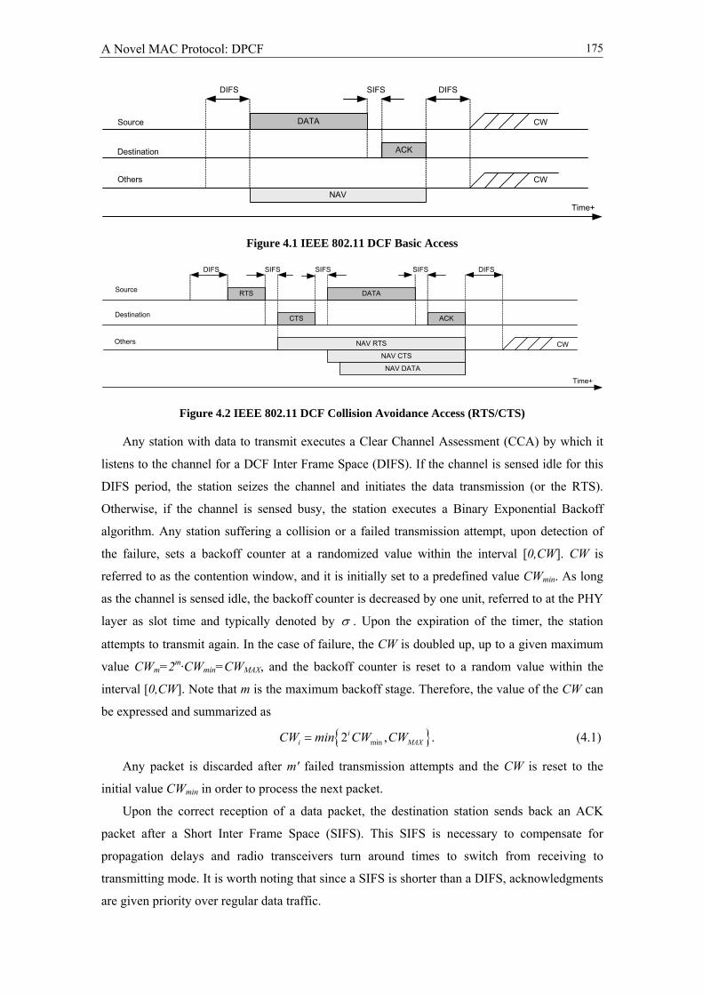
A Novel MAC Protocol: DPCF
175
DATA
ACK
Source
Destination
Others CW
NAV
DIFS SIFS DIFS
Time+
CW
Figure 4.1 IEEE 802.11 DCF Basic Access
DATA
ACK
Source
Destination
Others CW
DIFS
RTS
SIFS
CTS
SIFS
NAV RTS
NAV CTS
NAV DATA
DIFS
Time+
SIFS
Figure 4.2 IEEE 802.11 DCF Collision Avoidance Access (RTS/CTS)
Any station with data to transmit executes a Clear Channel Assessment (CCA) by which it
listens to the channel for a DCF Inter Frame Space (DIFS). If the channel is sensed idle for this
DIFS period, the station seizes the channel and initiates the data transmission (or the RTS).
Otherwise, if the channel is sensed busy, the station executes a Binary Exponential Backoff
algorithm. Any station suffering a collision or a failed transmission attempt, upon detection of
the failure, sets a backoff counter at a randomized value within the interval [0,CW]. CW is
referred to as the contention window, and it is initially set to a predefined value CWmin. As long
as the channel is sensed idle, the backoff counter is decreased by one unit, referred to at the PHY
layer as slot time and typically denoted by . Upon the expiration of the timer, the station
attempts to transmit again. In the case of failure, the CW is doubled up, up to a given maximum
value CWm=2m·CWmin=CWMAX, and the backoff counter is reset to a random value within the
interval [0,CW]. Note that m is the maximum backoff stage. Therefore, the value of the CW can
be expressed and summarized as
min2 , .ii MAXCW min CW CW (4.1)
Any packet is discarded after m' failed transmission attempts and the CW is reset to the
initial value CWmin in order to process the next packet.
Upon the correct reception of a data packet, the destination station sends back an ACK
packet after a Short Inter Frame Space (SIFS). This SIFS is necessary to compensate for
propagation delays and radio transceivers turn around times to switch from receiving to
transmitting mode. It is worth noting that since a SIFS is shorter than a DIFS, acknowledgments
are given priority over regular data traffic.
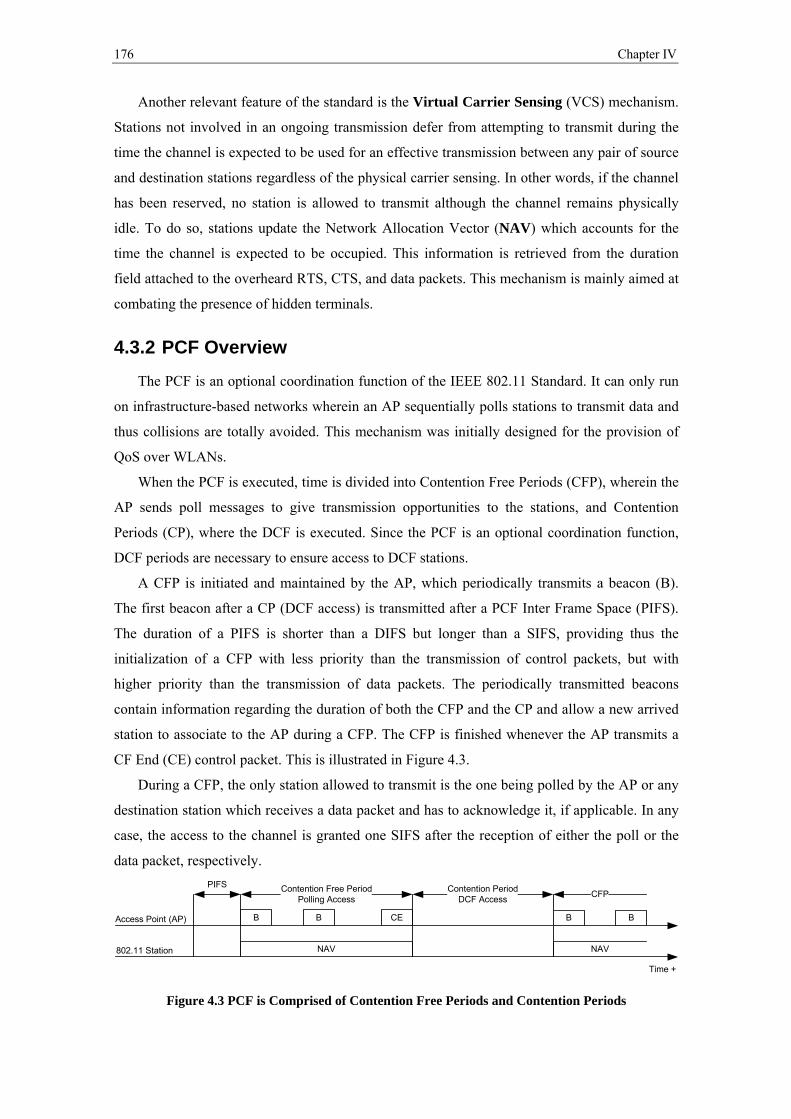
Chapter IV
176
Another relevant feature of the standard is the Virtual Carrier Sensing (VCS) mechanism.
Stations not involved in an ongoing transmission defer from attempting to transmit during the
time the channel is expected to be used for an effective transmission between any pair of source
and destination stations regardless of the physical carrier sensing. In other words, if the channel
has been reserved, no station is allowed to transmit although the channel remains physically
idle. To do so, stations update the Network Allocation Vector (NAV) which accounts for the
time the channel is expected to be occupied. This information is retrieved from the duration
field attached to the overheard RTS, CTS, and data packets. This mechanism is mainly aimed at
combating the presence of hidden terminals.
4.3.2 PCF Overview
The PCF is an optional coordination function of the IEEE 802.11 Standard. It can only run
on infrastructure-based networks wherein an AP sequentially polls stations to transmit data and
thus collisions are totally avoided. This mechanism was initially designed for the provision of
QoS over WLANs.
When the PCF is executed, time is divided into Contention Free Periods (CFP), wherein the
AP sends poll messages to give transmission opportunities to the stations, and Contention
Periods (CP), where the DCF is executed. Since the PCF is an optional coordination function,
DCF periods are necessary to ensure access to DCF stations.
A CFP is initiated and maintained by the AP, which periodically transmits a beacon (B).
The first beacon after a CP (DCF access) is transmitted after a PCF Inter Frame Space (PIFS).
The duration of a PIFS is shorter than a DIFS but longer than a SIFS, providing thus the
initialization of a CFP with less priority than the transmission of control packets, but with
higher priority than the transmission of data packets. The periodically transmitted beacons
contain information regarding the duration of both the CFP and the CP and allow a new arrived
station to associate to the AP during a CFP. The CFP is finished whenever the AP transmits a
CF End (CE) control packet. This is illustrated in Figure 4.3.
During a CFP, the only station allowed to transmit is the one being polled by the AP or any
destination station which receives a data packet and has to acknowledge it, if applicable. In any
case, the access to the channel is granted one SIFS after the reception of either the poll or the
data packet, respectively.
Contention Period DCF Access
Contention Free PeriodPolling Access
NAV
Access Point (AP)
802.11 Station
B CE
CFP
B
NAV
Time +
B B
PIFS
Figure 4.3 PCF is Comprised of Contention Free Periods and Contention Periods
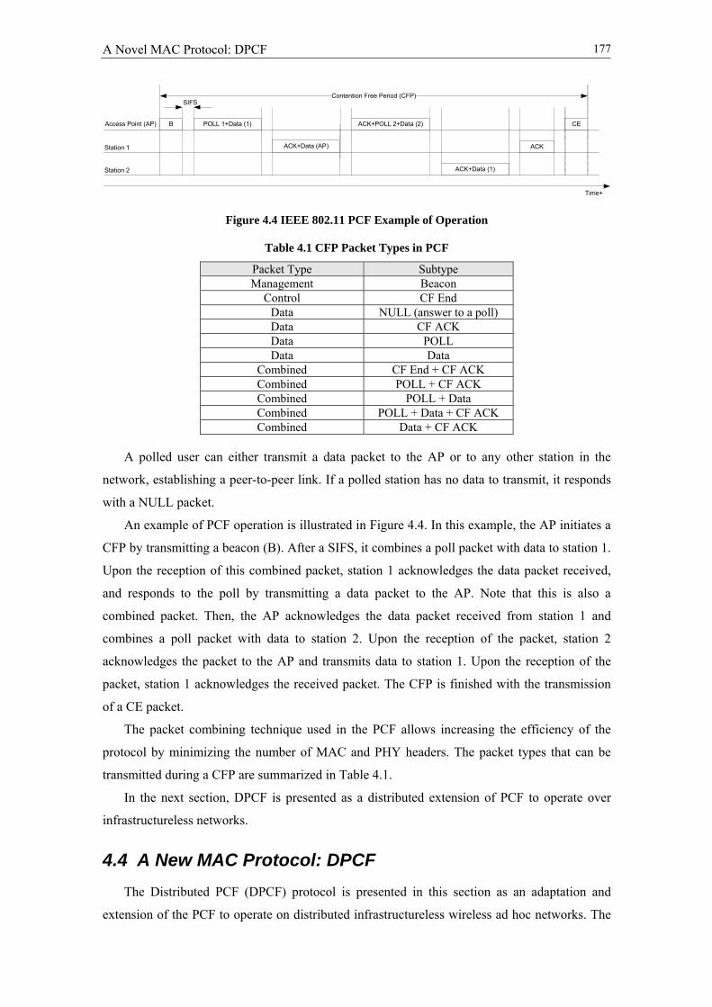
A Novel MAC Protocol: DPCF
177
Access Point (AP)
Station 1
Station 2
B POLL 1+Data (1)
Contention Free Period (CFP)SIFS
ACK+Data (AP)
ACK+POLL 2+Data (2)
ACK+Data (1)
ACK
CE
Time+
Figure 4.4 IEEE 802.11 PCF Example of Operation
Table 4.1 CFP Packet Types in PCF
Packet Type Subtype Management Beacon
Control CF End Data NULL (answer to a poll) Data CF ACK Data POLL Data Data
Combined CF End + CF ACK Combined POLL + CF ACK Combined POLL + Data Combined POLL + Data + CF ACK Combined Data + CF ACK
A polled user can either transmit a data packet to the AP or to any other station in the
network, establishing a peer-to-peer link. If a polled station has no data to transmit, it responds
with a NULL packet.
An example of PCF operation is illustrated in Figure 4.4. In this example, the AP initiates a
CFP by transmitting a beacon (B). After a SIFS, it combines a poll packet with data to station 1.
Upon the reception of this combined packet, station 1 acknowledges the data packet received,
and responds to the poll by transmitting a data packet to the AP. Note that this is also a
combined packet. Then, the AP acknowledges the data packet received from station 1 and
combines a poll packet with data to station 2. Upon the reception of the packet, station 2
acknowledges the packet to the AP and transmits data to station 1. Upon the reception of the
packet, station 1 acknowledges the received packet. The CFP is finished with the transmission
of a CE packet.
The packet combining technique used in the PCF allows increasing the efficiency of the
protocol by minimizing the number of MAC and PHY headers. The packet types that can be
transmitted during a CFP are summarized in Table 4.1.
In the next section, DPCF is presented as a distributed extension of PCF to operate over
infrastructureless networks.
4.4 A New MAC Protocol: DPCF
The Distributed PCF (DPCF) protocol is presented in this section as an adaptation and
extension of the PCF to operate on distributed infrastructureless wireless ad hoc networks. The
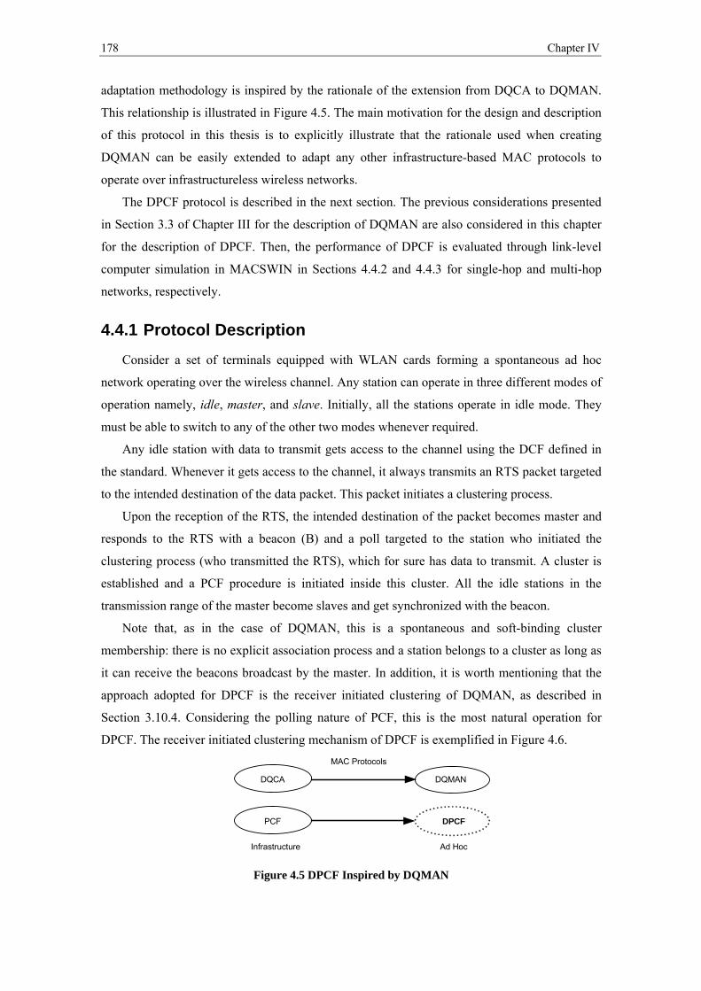
Chapter IV
178
adaptation methodology is inspired by the rationale of the extension from DQCA to DQMAN.
This relationship is illustrated in Figure 4.5. The main motivation for the design and description
of this protocol in this thesis is to explicitly illustrate that the rationale used when creating
DQMAN can be easily extended to adapt any other infrastructure-based MAC protocols to
operate over infrastructureless wireless networks.
The DPCF protocol is described in the next section. The previous considerations presented
in Section 3.3 of Chapter III for the description of DQMAN are also considered in this chapter
for the description of DPCF. Then, the performance of DPCF is evaluated through link-level
computer simulation in MACSWIN in Sections 4.4.2 and 4.4.3 for single-hop and multi-hop
networks, respectively.
4.4.1 Protocol Description
Consider a set of terminals equipped with WLAN cards forming a spontaneous ad hoc
network operating over the wireless channel. Any station can operate in three different modes of
operation namely, idle, master, and slave. Initially, all the stations operate in idle mode. They
must be able to switch to any of the other two modes whenever required.
Any idle station with data to transmit gets access to the channel using the DCF defined in
the standard. Whenever it gets access to the channel, it always transmits an RTS packet targeted
to the intended destination of the data packet. This packet initiates a clustering process.
Upon the reception of the RTS, the intended destination of the packet becomes master and
responds to the RTS with a beacon (B) and a poll targeted to the station who initiated the
clustering process (who transmitted the RTS), which for sure has data to transmit. A cluster is
established and a PCF procedure is initiated inside this cluster. All the idle stations in the
transmission range of the master become slaves and get synchronized with the beacon.
Note that, as in the case of DQMAN, this is a spontaneous and soft-binding cluster
membership: there is no explicit association process and a station belongs to a cluster as long as
it can receive the beacons broadcast by the master. In addition, it is worth mentioning that the
approach adopted for DPCF is the receiver initiated clustering of DQMAN, as described in
Section 3.10.4. Considering the polling nature of PCF, this is the most natural operation for
DPCF. The receiver initiated clustering mechanism of DPCF is exemplified in Figure 4.6.
DQMANDQCA
DPCFPCF
Infrastructure Ad Hoc
MAC Protocols
Figure 4.5 DPCF Inspired by DQMAN
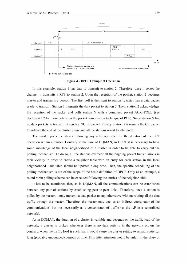
A Novel MAC Protocol: DPCF
179
ACK +POLL N
NULL
CE
RTS
B
Station 1
Cluster
PCF
POLL 1Station 2
SIFS
DATA for station 2
Station N
Time +
Station 2 becomes Master, and stations 1,3,…,N become Slave All the stations revert to idle mode
All the stations are idle
Figure 4.6 DPCF Example of Operation
In this example, station 1 has data to transmit to station 2. Therefore, once it seizes the
channel, it transmits a RTS to station 2. Upon the reception of the packet, station 2 becomes
master and transmits a beacon. The first poll is then sent to station 1, which has a data packet
ready to transmit. Station 1 transmits the data packet to station 2. Then, station 2 acknowledges
the reception of the packet and polls station N with a combined packet ACK+POLL (see
Section 4.3.2 for more details on the packet combination technique of PCF). Since station N has
no data packets to transmit, it sends a NULL packet. Finally, station 2 transmits the CE packet
to indicate the end of the cluster phase and all the stations revert to idle mode.
The master polls the slaves following any arbitrary order for the duration of the PCF
operation within a cluster. Contrary to the case of DQMAN, in DPCF it is necessary to have
some knowledge of the local neighborhood of a master in order to be able to carry out the
polling mechanism. To do so, all the stations overhear all the ongoing packet transmissions in
their vicinity in order to create a neighbor table with an entry for each station in the local
neighborhood. This table should be updated along time. Then, the specific scheduling of the
polling mechanism is out of the scope of the basic definition of DPCF. Only as an example, a
round robin polling scheme can be executed following the entries of the neighbor table.
It has to be mentioned that, as in DQMAN, all the communications can be established
between any pair of stations by establishing peer-to-peer links. Therefore, once a station is
polled by the master, it may transmit a data packet to any other slave without routing all the data
traffic through the master. Therefore, the master only acts as an indirect coordinator of the
communications, but not necessarily as a concentrator of traffic (as the AP in a centralized
network).
As in DQMAN, the duration of a cluster is variable and depends on the traffic load of the
network; a cluster is broken whenever there is no data activity in the network or, on the
contrary, when the traffic load is such that it would cause the cluster setting to remain static for
long (probably unbounded) periods of time. This latter situation would be unfair in the share of
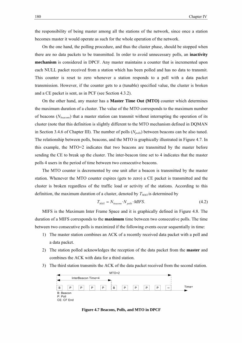
Chapter IV
180
the responsibility of being master among all the stations of the network, since once a station
becomes master it would operate as such for the whole operation of the network.
On the one hand, the polling procedure, and thus the cluster phase, should be stopped when
there are no data packets to be transmitted. In order to avoid unnecessary polls, an inactivity
mechanism is considered in DPCF. Any master maintains a counter that is incremented upon
each NULL packet received from a station which has been polled and has no data to transmit.
This counter is reset to zero whenever a station responds to a poll with a data packet
transmission. However, if the counter gets to a (tunable) specified value, the cluster is broken
and a CE packet is sent, as in PCF (see Section 4.3.2).
On the other hand, any master has a Master Time Out (MTO) counter which determines
the maximum duration of a cluster. The value of the MTO corresponds to the maximum number
of beacons (Nbeacons) that a master station can transmit without interrupting the operation of its
cluster (note that this definition is slightly different to the MTO mechanism defined in DQMAN
in Section 3.4.6 of Chapter III). The number of polls (Npolls) between beacons can be also tuned.
The relationship between polls, beacons, and the MTO is graphically illustrated in Figure 4.7. In
this example, the MTO=2 indicates that two beacons are transmitted by the master before
sending the CE to break up the cluster. The inter-beacon time set to 4 indicates that the master
polls 4 users in the period of time between two consecutive beacons.
The MTO counter is decremented by one unit after a beacon is transmitted by the master
station. Whenever the MTO counter expires (gets to zero) a CE packet is transmitted and the
cluster is broken regardless of the traffic load or activity of the stations. According to this
definition, the maximum duration of a cluster, denoted by TMAX is determined by
· · .MAX beacons pollsT N N MIFS (4.2)
MIFS is the Maximum Inter Frame Space and it is graphically defined in Figure 4.8. The
duration of a MIFS corresponds to the maximum time between two consecutive polls. The time
between two consecutive polls is maximized if the following events occur sequentially in time:
1) The master station combines an ACK of a recently received data packet with a poll and
a data packet.
2) The station polled acknowledges the reception of the data packet from the master and
combines the ACK with data for a third station.
3) The third station transmits the ACK of the data packet received from the second station.
B P P P P B P P P P CE
MTO=2
InterBeacon Time=4
Time+
B: BeaconP: PollCE: CF End
Figure 4.7 Beacons, Polls, and MTO in DPCF
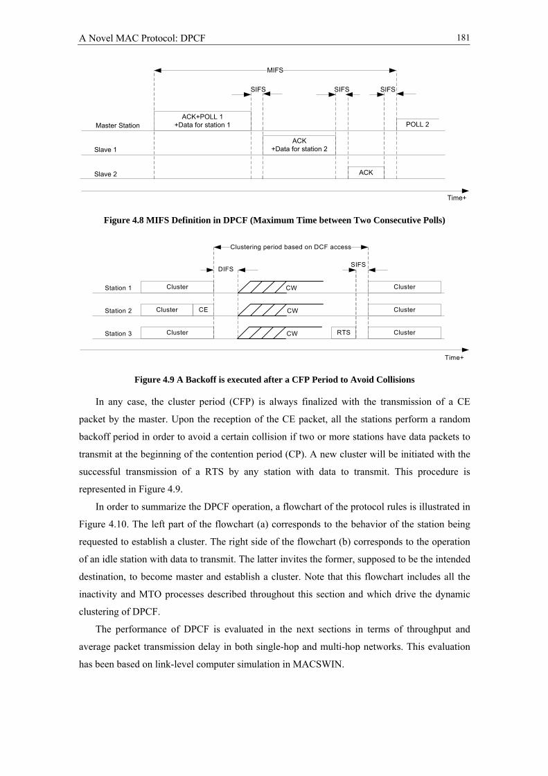
A Novel MAC Protocol: DPCF
181
Master Station
Slave 1
Slave 2
ACK+POLL 1+Data for station 1
SIFS
ACK+Data for station 2
ACK
SIFS SIFS
MIFS
POLL 2
Time+
Figure 4.8 MIFS Definition in DPCF (Maximum Time between Two Consecutive Polls)
ClusterStation 1
ClusterStation 2
ClusterStation 3
DIFS
RTS
Time+
CW
CW
CW Cluster
Cluster
Cluster
SIFS
Clustering period based on DCF access
CE
Figure 4.9 A Backoff is executed after a CFP Period to Avoid Collisions
In any case, the cluster period (CFP) is always finalized with the transmission of a CE
packet by the master. Upon the reception of the CE packet, all the stations perform a random
backoff period in order to avoid a certain collision if two or more stations have data packets to
transmit at the beginning of the contention period (CP). A new cluster will be initiated with the
successful transmission of a RTS by any station with data to transmit. This procedure is
represented in Figure 4.9.
In order to summarize the DPCF operation, a flowchart of the protocol rules is illustrated in
Figure 4.10. The left part of the flowchart (a) corresponds to the behavior of the station being
requested to establish a cluster. The right side of the flowchart (b) corresponds to the operation
of an idle station with data to transmit. The latter invites the former, supposed to be the intended
destination, to become master and establish a cluster. Note that this flowchart includes all the
inactivity and MTO processes described throughout this section and which drive the dynamic
clustering of DPCF.
The performance of DPCF is evaluated in the next sections in terms of throughput and
average packet transmission delay in both single-hop and multi-hop networks. This evaluation
has been based on link-level computer simulation in MACSWIN.
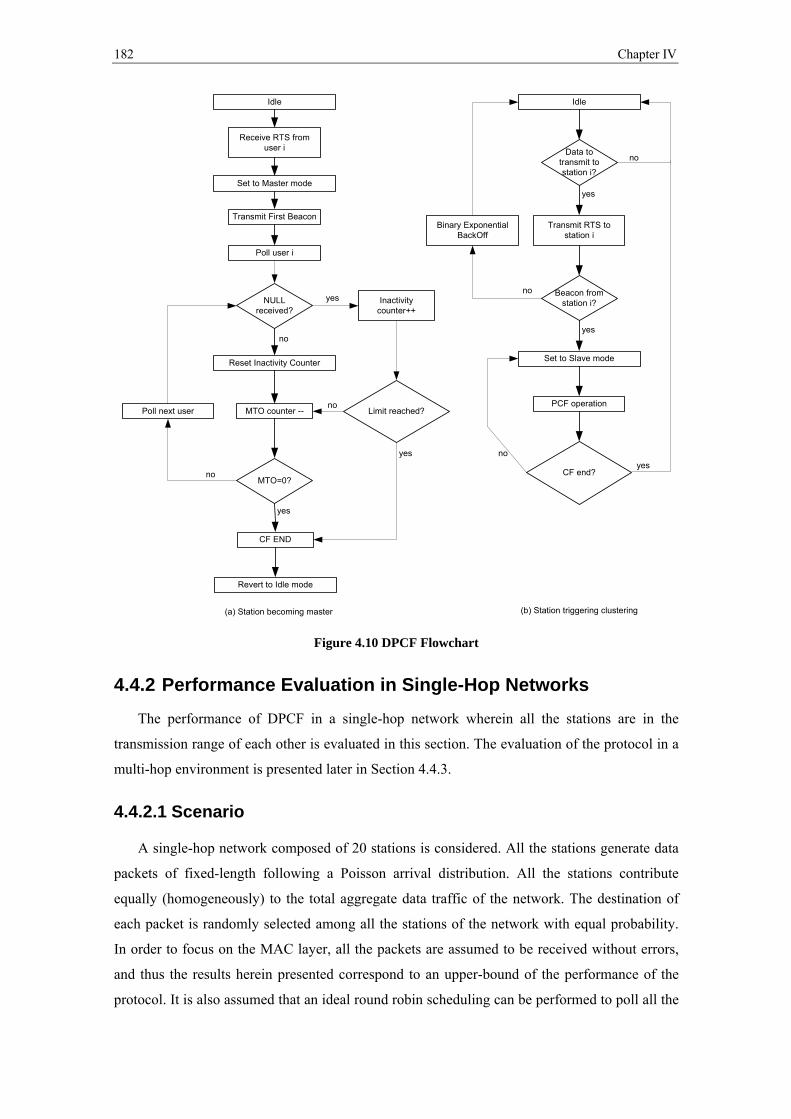
Chapter IV
182
Poll user i
NULL received?
Limit reached?
CF END
Inactivity counter++
MTO=0?
MTO counter --
Receive RTS from user i
Transmit First Beacon
Idle
Revert to Idle mode
Set to Master mode
yes
Poll next user
no
no
no
yes
yes
Idle
Data to transmit to station i?
Transmit RTS to station i
Beacon from station i?
Binary Exponential BackOff
Set to Slave mode
CF end?
PCF operation
yes
yes
yes
no
no
no
(b) Station triggering clustering(a) Station becoming master
Reset Inactivity Counter
Figure 4.10 DPCF Flowchart
4.4.2 Performance Evaluation in Single-Hop Networks
The performance of DPCF in a single-hop network wherein all the stations are in the
transmission range of each other is evaluated in this section. The evaluation of the protocol in a
multi-hop environment is presented later in Section 4.4.3.
4.4.2.1 Scenario
A single-hop network composed of 20 stations is considered. All the stations generate data
packets of fixed-length following a Poisson arrival distribution. All the stations contribute
equally (homogeneously) to the total aggregate data traffic of the network. The destination of
each packet is randomly selected among all the stations of the network with equal probability.
In order to focus on the MAC layer, all the packets are assumed to be received without errors,
and thus the results herein presented correspond to an upper-bound of the performance of the
protocol. It is also assumed that an ideal round robin scheduling can be performed to poll all the
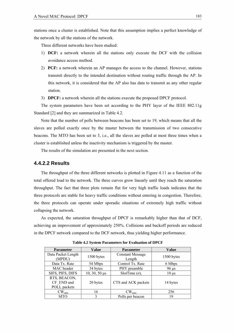
A Novel MAC Protocol: DPCF
183
stations once a cluster is established. Note that this assumption implies a perfect knowledge of
the network by all the stations of the network.
Three different networks have been studied:
1) DCF: a network wherein all the stations only execute the DCF with the collision
avoidance access method.
2) PCF: a network wherein an AP manages the access to the channel. However, stations
transmit directly to the intended destination without routing traffic through the AP. In
this network, it is considered that the AP also has data to transmit as any other regular
station.
3) DPCF: a network wherein all the stations execute the proposed DPCF protocol.
The system parameters have been set according to the PHY layer of the IEEE 802.11g
Standard [2] and they are summarized in Table 4.2.
Note that the number of polls between beacons has been set to 19, which means that all the
slaves are polled exactly once by the master between the transmission of two consecutive
beacons. The MTO has been set to 3, i.e., all the slaves are polled at most three times when a
cluster is established unless the inactivity mechanism is triggered by the master.
The results of the simulation are presented in the next section.
4.4.2.2 Results
The throughput of the three different networks is plotted in Figure 4.11 as a function of the
total offered load to the network. The three curves grow linearly until they reach the saturation
throughput. The fact that three plots remain flat for very high traffic loads indicates that the
three protocols are stable for heavy traffic conditions without entering in congestion. Therefore,
the three protocols can operate under sporadic situations of extremely high traffic without
collapsing the network.
As expected, the saturation throughput of DPCF is remarkably higher than that of DCF,
achieving an improvement of approximately 250%. Collisions and backoff periods are reduced
in the DPCF network compared to the DCF network, thus yielding higher performance.
Table 4.2 System Parameters for Evaluation of DPCF
Parameter Value Parameter Value Data Packet Length
(MPDU) 1500 bytes
Constant Message Length
1500 bytes
Data Tx. Rate 54 Mbps Control Tx. Rate 6 Mbps MAC header 34 bytes PHY preamble 96 μs
SIFS, PIFS, DIFS 10, 30, 50 μs SlotTime (σ), 10 μs RTS, BEACON,
CF_END and POLL packets
20 bytes CTS and ACK packets 14 bytes
CWmin 16 CWmax 256 MTO 3 Polls per beacon 19
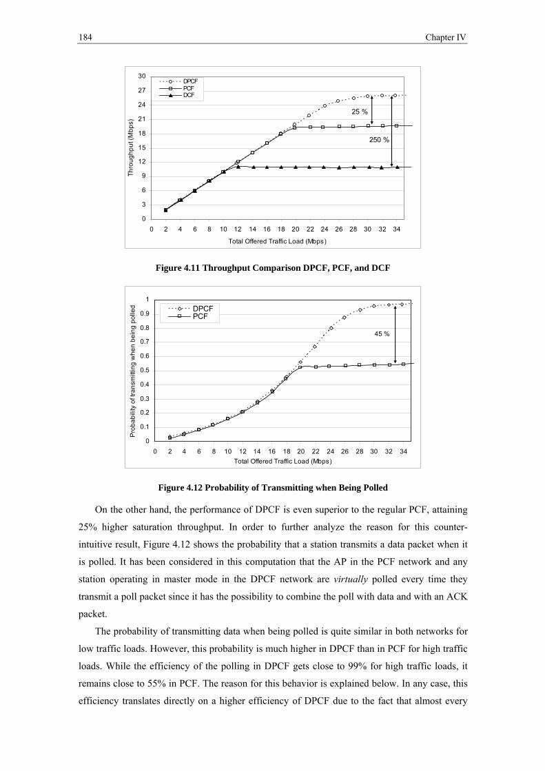
Chapter IV
184
0
3
6
9
12
15
18
21
24
27
30
0 2 4 6 8 10 12 14 16 18 20 22 24 26 28 30 32 34
Total Offered Traffic Load (Mbps)
Th
rou
gh
pu
t (M
bp
s)
DPCFPCFDCF
25 %
250 %
Figure 4.11 Throughput Comparison DPCF, PCF, and DCF
0
0.1
0.2
0.3
0.4
0.5
0.6
0.7
0.8
0.9
1
0 2 4 6 8 10 12 14 16 18 20 22 24 26 28 30 32 34
Total Offered Traffic Load (Mbps)
Pro
ba
bili
ty o
f tra
nsm
ittin
g w
he
n b
ein
g p
olle
d DPCFPCF
45 %
Figure 4.12 Probability of Transmitting when Being Polled
On the other hand, the performance of DPCF is even superior to the regular PCF, attaining
25% higher saturation throughput. In order to further analyze the reason for this counter-
intuitive result, Figure 4.12 shows the probability that a station transmits a data packet when it
is polled. It has been considered in this computation that the AP in the PCF network and any
station operating in master mode in the DPCF network are virtually polled every time they
transmit a poll packet since it has the possibility to combine the poll with data and with an ACK
packet.
The probability of transmitting data when being polled is quite similar in both networks for
low traffic loads. However, this probability is much higher in DPCF than in PCF for high traffic
loads. While the efficiency of the polling in DPCF gets close to 99% for high traffic loads, it
remains close to 55% in PCF. The reason for this behavior is explained below. In any case, this
efficiency translates directly on a higher efficiency of DPCF due to the fact that almost every
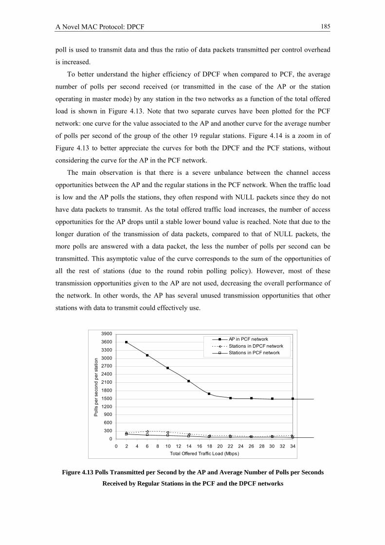
A Novel MAC Protocol: DPCF
185
poll is used to transmit data and thus the ratio of data packets transmitted per control overhead
is increased.
To better understand the higher efficiency of DPCF when compared to PCF, the average
number of polls per second received (or transmitted in the case of the AP or the station
operating in master mode) by any station in the two networks as a function of the total offered
load is shown in Figure 4.13. Note that two separate curves have been plotted for the PCF
network: one curve for the value associated to the AP and another curve for the average number
of polls per second of the group of the other 19 regular stations. Figure 4.14 is a zoom in of
Figure 4.13 to better appreciate the curves for both the DPCF and the PCF stations, without
considering the curve for the AP in the PCF network.
The main observation is that there is a severe unbalance between the channel access
opportunities between the AP and the regular stations in the PCF network. When the traffic load
is low and the AP polls the stations, they often respond with NULL packets since they do not
have data packets to transmit. As the total offered traffic load increases, the number of access
opportunities for the AP drops until a stable lower bound value is reached. Note that due to the
longer duration of the transmission of data packets, compared to that of NULL packets, the
more polls are answered with a data packet, the less the number of polls per second can be
transmitted. This asymptotic value of the curve corresponds to the sum of the opportunities of
all the rest of stations (due to the round robin polling policy). However, most of these
transmission opportunities given to the AP are not used, decreasing the overall performance of
the network. In other words, the AP has several unused transmission opportunities that other
stations with data to transmit could effectively use.
0
300
600
900
1200
1500
1800
2100
2400
2700
3000
3300
3600
3900
0 2 4 6 8 10 12 14 16 18 20 22 24 26 28 30 32 34
Total Offered Traffic Load (Mbps)
Po
lls p
er
seco
nd
pe
r st
atio
n
AP in PCF network
Stations in DPCF network
Stations in PCF network
Figure 4.13 Polls Transmitted per Second by the AP and Average Number of Polls per Seconds
Received by Regular Stations in the PCF and the DPCF networks
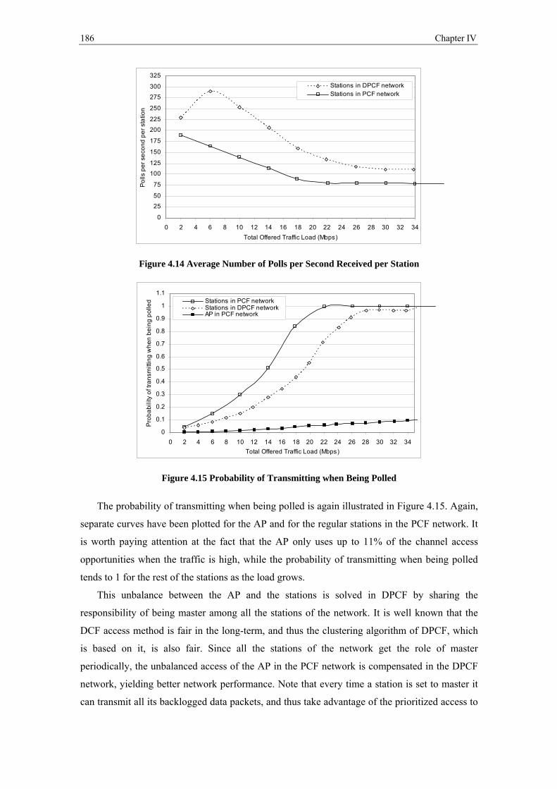
Chapter IV
186
0
25
50
75
100
125
150
175
200
225
250
275
300
325
0 2 4 6 8 10 12 14 16 18 20 22 24 26 28 30 32 34
Total Offered Traffic Load (Mbps)
Po
lls p
er
seco
nd
pe
r st
atio
n
Stations in DPCF networkStations in PCF network
Figure 4.14 Average Number of Polls per Second Received per Station
0
0.1
0.2
0.3
0.4
0.5
0.6
0.7
0.8
0.9
1
1.1
0 2 4 6 8 10 12 14 16 18 20 22 24 26 28 30 32 34
Total Offered Traffic Load (Mbps)
Pro
ba
bili
ty o
f tra
nsm
ittin
g w
he
n b
ein
g p
olle
d Stations in PCF networkStations in DPCF networkAP in PCF network
Figure 4.15 Probability of Transmitting when Being Polled
The probability of transmitting when being polled is again illustrated in Figure 4.15. Again,
separate curves have been plotted for the AP and for the regular stations in the PCF network. It
is worth paying attention at the fact that the AP only uses up to 11% of the channel access
opportunities when the traffic is high, while the probability of transmitting when being polled
tends to 1 for the rest of the stations as the load grows.
This unbalance between the AP and the stations is solved in DPCF by sharing the
responsibility of being master among all the stations of the network. It is well known that the
DCF access method is fair in the long-term, and thus the clustering algorithm of DPCF, which
is based on it, is also fair. Since all the stations of the network get the role of master
periodically, the unbalanced access of the AP in the PCF network is compensated in the DPCF
network, yielding better network performance. Note that every time a station is set to master it
can transmit all its backlogged data packets, and thus take advantage of the prioritized access to
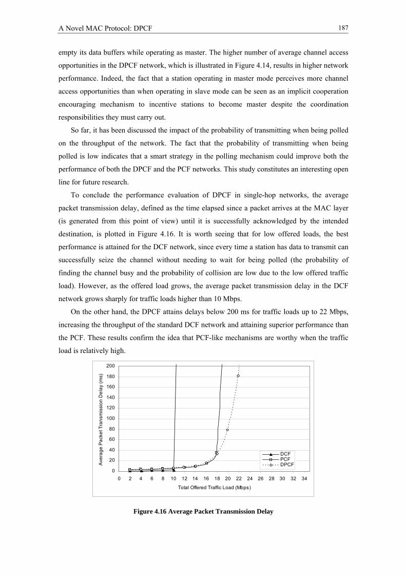
A Novel MAC Protocol: DPCF
187
empty its data buffers while operating as master. The higher number of average channel access
opportunities in the DPCF network, which is illustrated in Figure 4.14, results in higher network
performance. Indeed, the fact that a station operating in master mode perceives more channel
access opportunities than when operating in slave mode can be seen as an implicit cooperation
encouraging mechanism to incentive stations to become master despite the coordination
responsibilities they must carry out.
So far, it has been discussed the impact of the probability of transmitting when being polled
on the throughput of the network. The fact that the probability of transmitting when being
polled is low indicates that a smart strategy in the polling mechanism could improve both the
performance of both the DPCF and the PCF networks. This study constitutes an interesting open
line for future research.
To conclude the performance evaluation of DPCF in single-hop networks, the average
packet transmission delay, defined as the time elapsed since a packet arrives at the MAC layer
(is generated from this point of view) until it is successfully acknowledged by the intended
destination, is plotted in Figure 4.16. It is worth seeing that for low offered loads, the best
performance is attained for the DCF network, since every time a station has data to transmit can
successfully seize the channel without needing to wait for being polled (the probability of
finding the channel busy and the probability of collision are low due to the low offered traffic
load). However, as the offered load grows, the average packet transmission delay in the DCF
network grows sharply for traffic loads higher than 10 Mbps.
On the other hand, the DPCF attains delays below 200 ms for traffic loads up to 22 Mbps,
increasing the throughput of the standard DCF network and attaining superior performance than
the PCF. These results confirm the idea that PCF-like mechanisms are worthy when the traffic
load is relatively high.
0
20
40
60
80
100
120
140
160
180
200
0 2 4 6 8 10 12 14 16 18 20 22 24 26 28 30 32 34
Total Offered Traffic Load (Mbps)
Ave
rag
e P
ack
et T
ran
smis
sio
n D
ela
y (m
s)
DCFPCFDPCF
Figure 4.16 Average Packet Transmission Delay
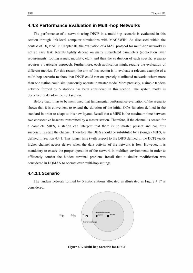
Chapter IV
188
4.4.3 Performance Evaluation in Multi-hop Networks
The performance of a network using DPCF in a multi-hop scenario is evaluated in this
section through link-level computer simulations with MACSWIN. As discussed within the
context of DQMAN in Chapter III, the evaluation of a MAC protocol for multi-hop networks is
not an easy task. Results tightly depend on many interrelated parameters (application layer
requirements, routing issues, mobility, etc.), and thus the evaluation of each specific scenario
requires a particular approach. Furthermore, each application might require the evaluation of
different metrics. For this reason, the aim of this section is to evaluate a relevant example of a
multi-hop scenario to show that DPCF could run on sparsely distributed networks where more
than one station could simultaneously operate in master mode. More precisely, a simple tandem
network formed by 5 stations has been considered in this section. The system model is
described in detail in the next section.
Before that, it has to be mentioned that fundamental performance evaluation of the scenario
shows that it is convenient to extend the duration of the initial CCA function defined in the
standard in order to adapt to this new layout. Recall that a MIFS is the maximum time between
two consecutive beacons transmitted by a master station. Therefore, if the channel is sensed for
a complete MIFS, a station can interpret that there is no master present and can thus
successfully seize the channel. Therefore, the DIFS should be substituted by a (longer) MIFS, as
defined in Section 4.4.1. This longer time (with respect to the DIFS defined in the DCF) yields
higher channel access delays when the data activity of the network is low. However, it is
mandatory to ensure the proper operation of the network in multihop environments in order to
efficiently combat the hidden terminal problem. Recall that a similar modification was
considered in DQMAN to operate over multi-hop settings.
4.4.3.1 Scenario
The tandem network formed by 5 static stations allocated as illustrated in Figure 4.17 is
considered.
IDLE
Transmission Range
Interference Range
SLAVE MASTERIDLEIDLE
Figure 4.17 Multi-hop Scenario for DPCF
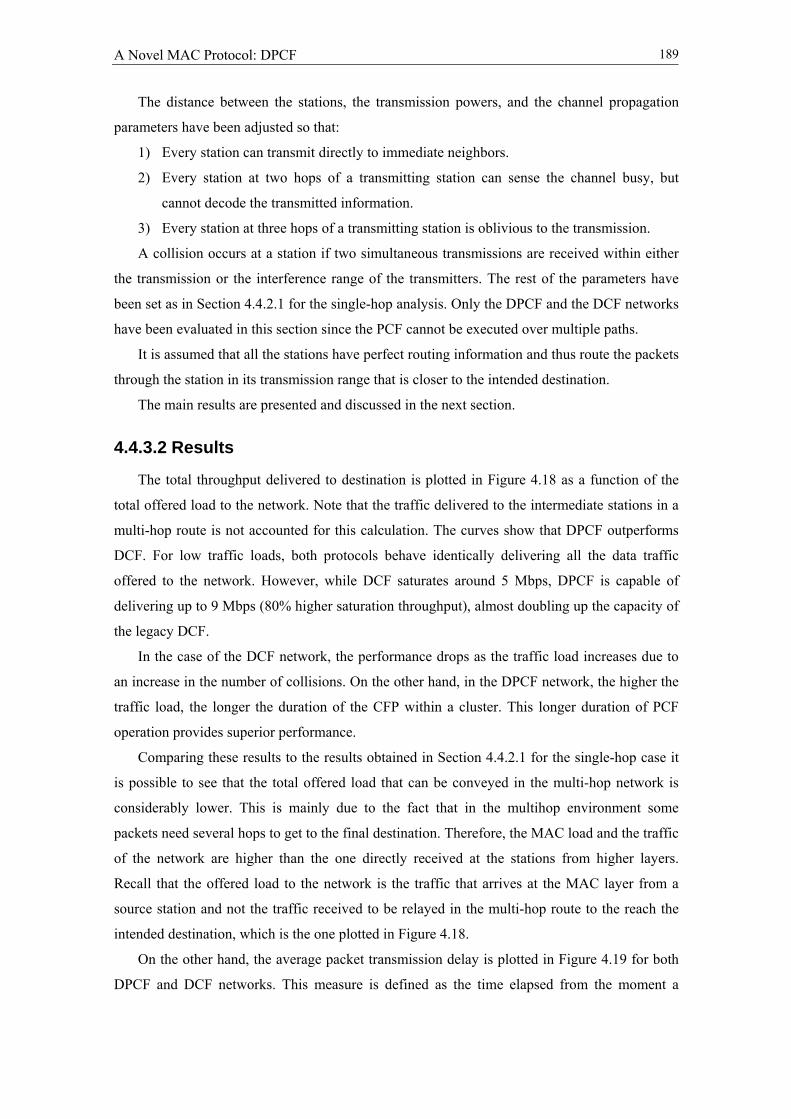
A Novel MAC Protocol: DPCF
189
The distance between the stations, the transmission powers, and the channel propagation
parameters have been adjusted so that:
1) Every station can transmit directly to immediate neighbors.
2) Every station at two hops of a transmitting station can sense the channel busy, but
cannot decode the transmitted information.
3) Every station at three hops of a transmitting station is oblivious to the transmission.
A collision occurs at a station if two simultaneous transmissions are received within either
the transmission or the interference range of the transmitters. The rest of the parameters have
been set as in Section 4.4.2.1 for the single-hop analysis. Only the DPCF and the DCF networks
have been evaluated in this section since the PCF cannot be executed over multiple paths.
It is assumed that all the stations have perfect routing information and thus route the packets
through the station in its transmission range that is closer to the intended destination.
The main results are presented and discussed in the next section.
4.4.3.2 Results
The total throughput delivered to destination is plotted in Figure 4.18 as a function of the
total offered load to the network. Note that the traffic delivered to the intermediate stations in a
multi-hop route is not accounted for this calculation. The curves show that DPCF outperforms
DCF. For low traffic loads, both protocols behave identically delivering all the data traffic
offered to the network. However, while DCF saturates around 5 Mbps, DPCF is capable of
delivering up to 9 Mbps (80% higher saturation throughput), almost doubling up the capacity of
the legacy DCF.
In the case of the DCF network, the performance drops as the traffic load increases due to
an increase in the number of collisions. On the other hand, in the DPCF network, the higher the
traffic load, the longer the duration of the CFP within a cluster. This longer duration of PCF
operation provides superior performance.
Comparing these results to the results obtained in Section 4.4.2.1 for the single-hop case it
is possible to see that the total offered load that can be conveyed in the multi-hop network is
considerably lower. This is mainly due to the fact that in the multihop environment some
packets need several hops to get to the final destination. Therefore, the MAC load and the traffic
of the network are higher than the one directly received at the stations from higher layers.
Recall that the offered load to the network is the traffic that arrives at the MAC layer from a
source station and not the traffic received to be relayed in the multi-hop route to the reach the
intended destination, which is the one plotted in Figure 4.18.
On the other hand, the average packet transmission delay is plotted in Figure 4.19 for both
DPCF and DCF networks. This measure is defined as the time elapsed from the moment a
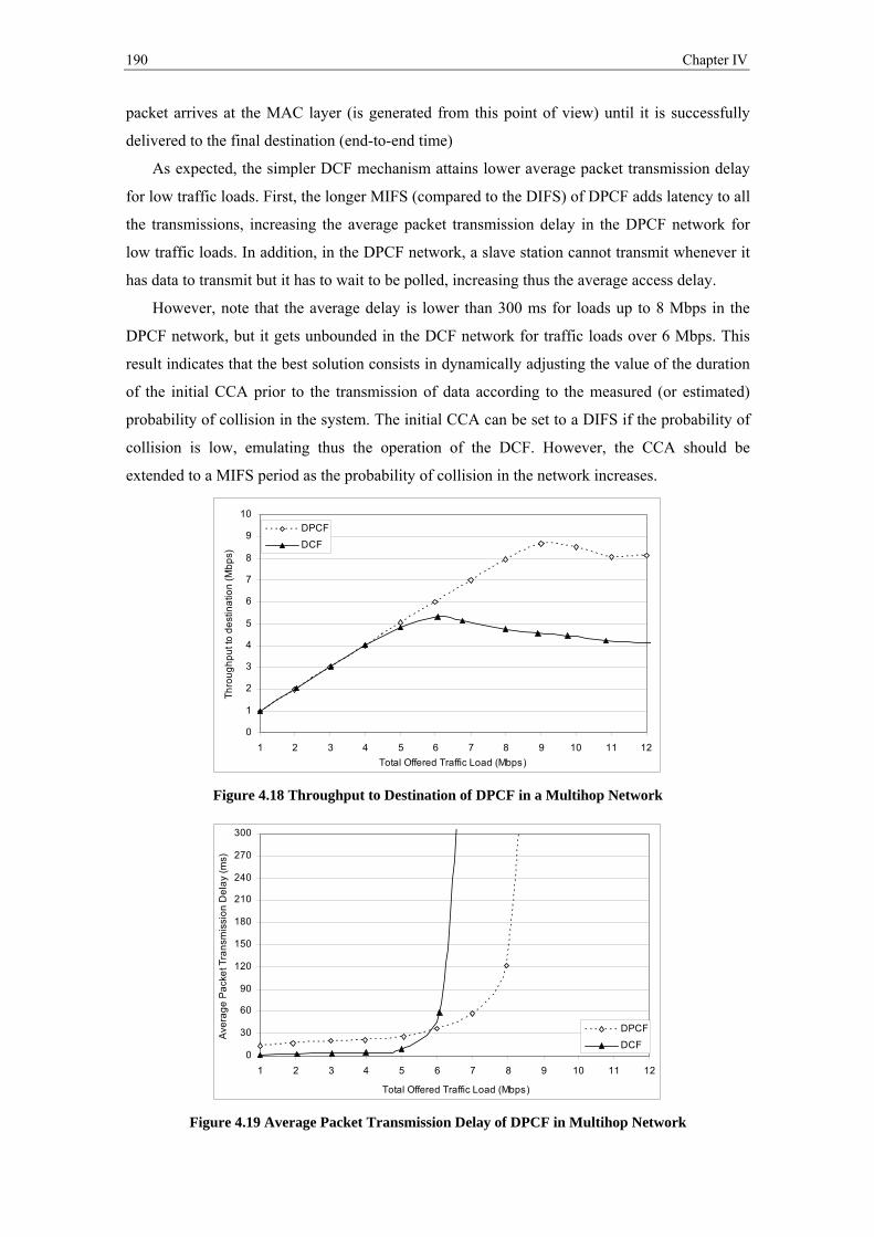
Chapter IV
190
packet arrives at the MAC layer (is generated from this point of view) until it is successfully
delivered to the final destination (end-to-end time)
As expected, the simpler DCF mechanism attains lower average packet transmission delay
for low traffic loads. First, the longer MIFS (compared to the DIFS) of DPCF adds latency to all
the transmissions, increasing the average packet transmission delay in the DPCF network for
low traffic loads. In addition, in the DPCF network, a slave station cannot transmit whenever it
has data to transmit but it has to wait to be polled, increasing thus the average access delay.
However, note that the average delay is lower than 300 ms for loads up to 8 Mbps in the
DPCF network, but it gets unbounded in the DCF network for traffic loads over 6 Mbps. This
result indicates that the best solution consists in dynamically adjusting the value of the duration
of the initial CCA prior to the transmission of data according to the measured (or estimated)
probability of collision in the system. The initial CCA can be set to a DIFS if the probability of
collision is low, emulating thus the operation of the DCF. However, the CCA should be
extended to a MIFS period as the probability of collision in the network increases.
0
1
2
3
4
5
6
7
8
9
10
1 2 3 4 5 6 7 8 9 10 11 12
Total Offered Traffic Load (Mbps)
Th
rou
gh
pu
t to
de
stin
atio
n (
Mb
ps)
DPCF
DCF
Figure 4.18 Throughput to Destination of DPCF in a Multihop Network
0
30
60
90
120
150
180
210
240
270
300
1 2 3 4 5 6 7 8 9 10 11 12
Total Offered Traffic Load (Mbps)
Ave
rag
e P
ack
et T
ran
smis
sio
n D
ela
y (m
s)
DPCF
DCF
Figure 4.19 Average Packet Transmission Delay of DPCF in Multihop Network
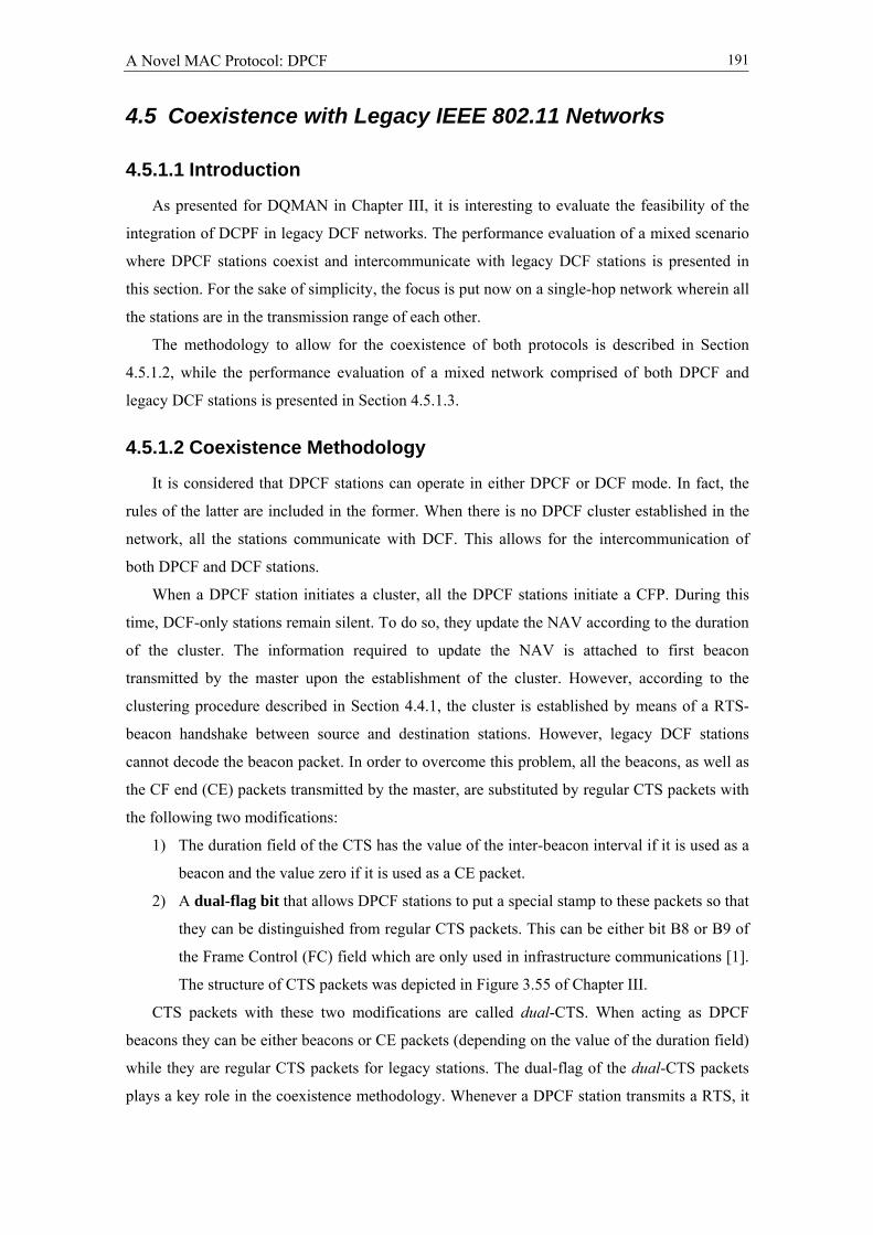
A Novel MAC Protocol: DPCF
191
4.5 Coexistence with Legacy IEEE 802.11 Networks
4.5.1.1 Introduction
As presented for DQMAN in Chapter III, it is interesting to evaluate the feasibility of the
integration of DCPF in legacy DCF networks. The performance evaluation of a mixed scenario
where DPCF stations coexist and intercommunicate with legacy DCF stations is presented in
this section. For the sake of simplicity, the focus is put now on a single-hop network wherein all
the stations are in the transmission range of each other.
The methodology to allow for the coexistence of both protocols is described in Section
4.5.1.2, while the performance evaluation of a mixed network comprised of both DPCF and
legacy DCF stations is presented in Section 4.5.1.3.
4.5.1.2 Coexistence Methodology
It is considered that DPCF stations can operate in either DPCF or DCF mode. In fact, the
rules of the latter are included in the former. When there is no DPCF cluster established in the
network, all the stations communicate with DCF. This allows for the intercommunication of
both DPCF and DCF stations.
When a DPCF station initiates a cluster, all the DPCF stations initiate a CFP. During this
time, DCF-only stations remain silent. To do so, they update the NAV according to the duration
of the cluster. The information required to update the NAV is attached to first beacon
transmitted by the master upon the establishment of the cluster. However, according to the
clustering procedure described in Section 4.4.1, the cluster is established by means of a RTS-
beacon handshake between source and destination stations. However, legacy DCF stations
cannot decode the beacon packet. In order to overcome this problem, all the beacons, as well as
the CF end (CE) packets transmitted by the master, are substituted by regular CTS packets with
the following two modifications:
1) The duration field of the CTS has the value of the inter-beacon interval if it is used as a
beacon and the value zero if it is used as a CE packet.
2) A dual-flag bit that allows DPCF stations to put a special stamp to these packets so that
they can be distinguished from regular CTS packets. This can be either bit B8 or B9 of
the Frame Control (FC) field which are only used in infrastructure communications [1].
The structure of CTS packets was depicted in Figure 3.55 of Chapter III.
CTS packets with these two modifications are called dual-CTS. When acting as DPCF
beacons they can be either beacons or CE packets (depending on the value of the duration field)
while they are regular CTS packets for legacy stations. The dual-flag of the dual-CTS packets
plays a key role in the coexistence methodology. Whenever a DPCF station transmits a RTS, it
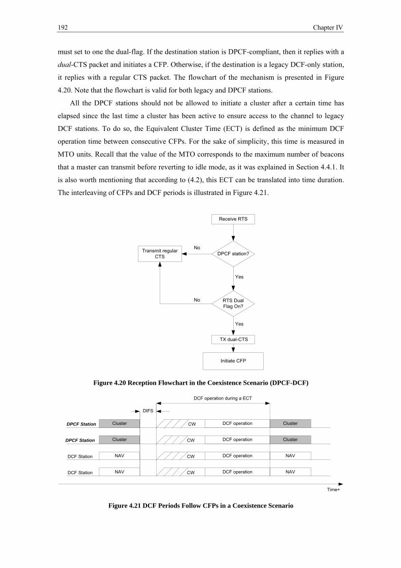
Chapter IV
192
must set to one the dual-flag. If the destination station is DPCF-compliant, then it replies with a
dual-CTS packet and initiates a CFP. Otherwise, if the destination is a legacy DCF-only station,
it replies with a regular CTS packet. The flowchart of the mechanism is presented in Figure
4.20. Note that the flowchart is valid for both legacy and DPCF stations.
All the DPCF stations should not be allowed to initiate a cluster after a certain time has
elapsed since the last time a cluster has been active to ensure access to the channel to legacy
DCF stations. To do so, the Equivalent Cluster Time (ECT) is defined as the minimum DCF
operation time between consecutive CFPs. For the sake of simplicity, this time is measured in
MTO units. Recall that the value of the MTO corresponds to the maximum number of beacons
that a master can transmit before reverting to idle mode, as it was explained in Section 4.4.1. It
is also worth mentioning that according to (4.2), this ECT can be translated into time duration.
The interleaving of CFPs and DCF periods is illustrated in Figure 4.21.
Receive RTS
DPCF station?
RTS Dual Flag On?
Transmit regular CTS
TX dual-CTS
No
Yes
No
Yes
Initiate CFP
Figure 4.20 Reception Flowchart in the Coexistence Scenario (DPCF-DCF)
ClusterDPCF Station
Cluster
NAV
DIFS
DCF operation during a ECT
CW
CW
CW DCF operation
DCF operation
DCF operation
Cluster
Cluster
NAV
Time+
NAV CW DCF operation NAV
DPCF Station
DCF Station
DCF Station
Figure 4.21 DCF Periods Follow CFPs in a Coexistence Scenario
A Novel MAC Protocol: DPCF
193
In this example, the operation of a network with 4 stations is represented. Two of them are
dual DPCF stations, while the other two are DCF stations. At the beginning of the time line
represented in the example, the two DPCF stations run the PCF (one of them must be operating
in master mode), while the other 2 DCF-only stations remain silent and update the NAV
according to the data and control packets transmitted during the cluster phase. Whenever the
cluster is broken up, and after a DIFS, all the stations perform a random backoff deferral period.
Then, and for the duration of the ECT, all the stations, including DPCF stations, get access to
the channel by executing the rules of the DCF of the standard. At the end of the ECT time, once
any of the two DPCF station seizes the channel, it initiates a cluster and the PCF can be
executed again. DCF-only stations update the NAV and refrain from attempting to get access to
the channel for the duration of the cluster.
It should be mentioned that the “forced” DCF periods can be used by DPCF stations to
overhear ongoing transmissions and learn the composition of the network in order to optimize
the polling policy whenever a CFP is initiated. In addition, recall that DPCF stations can access
the channel during these periods executing the rules of the DCF to transmit their data.
4.5.1.3 Performance Evaluation
4.5.1.3.1 Scenario
A network formed by a total of 20 stations in a single-hop scenario wherein all the stations
are in the transmission range of each other has been simulated with MACSWIN. 5 out of these
20 stations are dual DPCF stations and the other 15 stations are legacy DCF-only stations. All
the stations use the collision avoidance access method of the standard (with RTS/CTS
handshake).
The rest of the configuration parameters have been set as in Section 4.4.2.1 for the single-
hop performance evaluation of DPCF but with the following modifications: it has been
considered that DPCF stations transmit 16 poll packets in between two consecutive beacons,
and the MTO has been set to 4, i.e., at most a master sends 4 beacons before breaking the
cluster.
In addition, the results presented in the next section are compared in all cases to those of
two networks wherein all the 20 stations operate with only either the DPCF (without DCF
periods) or the DCF, respectively.
4.5.1.3.2 Results
The throughput as a function of the total offered traffic load is illustrated in Figure 4.22
when the ECT=1, i.e., the duration of the forced DCF operation after a DPCF cluster is equal to
the maximum duration of the cluster time.
Chapter IV
194
As shown in the figure, the performance of the mixed network lies in between the
performance of the DCF and the DPCF networks. Since both protocols are alternately executed
in a mixed network, the result is an intermediate performance. Therefore, the main conclusion is
that the mixed network works properly and thus coexistence, intercommunication, and smooth
migration to the new system is feasible. This result is very important in the light of the potential
commercial success of DPCF.
However, it is interesting to analyze, on the one hand, which performance is perceived by
the group of DPCF and DCF stations separately, as well as to consider the effect of using
different values for the ECT. To do so, the throughput of the group of 15 DCF stations is
illustrated in Figure 4.23, while the performance of the group of 5 DPCF stations is illustrated
in Figure 4.24. As a benchmark performance, the curve labeled with “DCF operation”
corresponds to the situation where only the DCF is executed and there are no CFPs. Note that
the values of the x-axis in these curves correspond to the total offered traffic load considering
the contribution of all the stations regardless of whether they are DCF-only or DPCF stations.
It is worth seeing that the performances perceived by each group of stations are
complementary. As the value of the ECT increases, i.e., longer DCF periods are allowed, the
performance of the DCF-only stations increases, as expected. In the limit, where the DCF tends
to be the only access method used by all the stations (including the dual DPCF stations), the
performance of the DCF-only group of stations is exactly ¾ of the total throughput of the
network (15 out of 20 stations). This is due to the well known long-term fairness of the DCF.
On the other hand, the throughput perceived by the group of DPCF stations is higher as the
value of the ECT becomes smaller. A smaller value of the ECT allows the occurrence of longer
CFPs with shorter DCF periods in between, where the performance is much higher than during
DCF periods. It is worth noting that the performance of the DPCF stations can increase up to
400% when the ECT=3 with respect to the case of only executing the DCF.
On the other hand, the average packet transmission delay of the network as a function of the
total offered load to the network is illustrated in Figure 4.25 (no distinction between DPCF and
DCF stations has been considered in this figure but the overall average has been calculated).
For low traffic loads, the delay of the mixed scenario is similar to that of the DCF network.
However, as the traffic load grows, the delay of the mixed scenario grows sharply. This is due
to the fact that DCF stations suffer long access delays when CFPs occur frequently and they
have to wait for the DCF period to get access to the channel. Recall that DCF stations can only
transmit data during DCF periods.
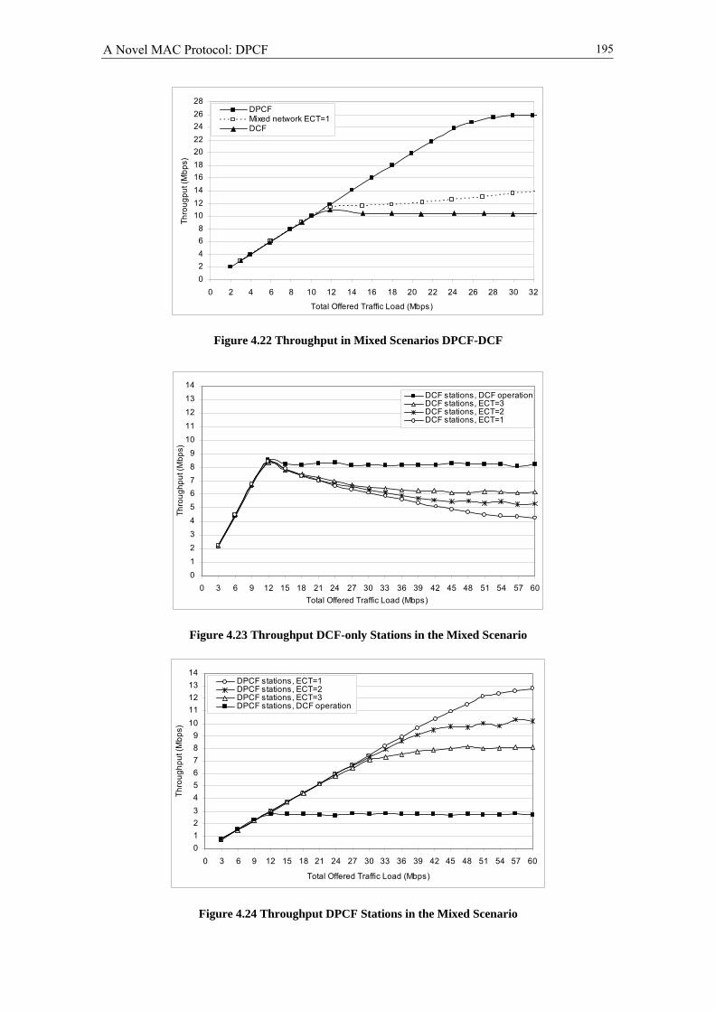
A Novel MAC Protocol: DPCF
195
0
2
4
6
8
10
12
14
16
18
20
22
24
26
28
0 2 4 6 8 10 12 14 16 18 20 22 24 26 28 30 32
Total Offered Traffic Load (Mbps)
Th
rou
gp
ut (
Mb
ps)
DPCFMixed network ECT=1DCF
Figure 4.22 Throughput in Mixed Scenarios DPCF-DCF
0
1
2
3
4
5
6
7
8
9
10
11
12
13
14
0 3 6 9 12 15 18 21 24 27 30 33 36 39 42 45 48 51 54 57 60
Total Offered Traffic Load (Mbps)
Th
rou
gh
pu
t (M
bp
s)
DCF stations, DCF operationDCF stations, ECT=3DCF stations, ECT=2DCF stations, ECT=1
Figure 4.23 Throughput DCF-only Stations in the Mixed Scenario
0
1
2
3
4
5
6
7
8
9
10
11
12
13
14
0 3 6 9 12 15 18 21 24 27 30 33 36 39 42 45 48 51 54 57 60
Total Offered Traffic Load (Mbps)
Th
rou
gh
pu
t (M
bp
s)
DPCF stations, ECT=1DPCF stations, ECT=2DPCF stations, ECT=3DPCF stations, DCF operation
Figure 4.24 Throughput DPCF Stations in the Mixed Scenario
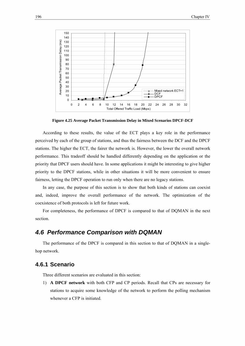
Chapter IV
196
0
10
20
30
40
50
60
70
80
90
100
110
120
130
140
150
0 2 4 6 8 10 12 14 16 18 20 22 24 26 28 30 32
Total Offered Traffic Load (Mbps)
Ave
rag
e P
ack
et T
ran
smis
sio
n D
ela
y (m
s)
Mixed network ECT=1DCFDPCF
Figure 4.25 Average Packet Transmission Delay in Mixed Scenarios DPCF-DCF
According to these results, the value of the ECT plays a key role in the performance
perceived by each of the group of stations, and thus the fairness between the DCF and the DPCF
stations. The higher the ECT, the fairer the network is. However, the lower the overall network
performance. This tradeoff should be handled differently depending on the application or the
priority that DPCF users should have. In some applications it might be interesting to give higher
priority to the DPCF stations, while in other situations it will be more convenient to ensure
fairness, letting the DPCF operation to run only when there are no legacy stations.
In any case, the purpose of this section is to show that both kinds of stations can coexist
and, indeed, improve the overall performance of the network. The optimization of the
coexistence of both protocols is left for future work.
For completeness, the performance of DPCF is compared to that of DQMAN in the next
section.
4.6 Performance Comparison with DQMAN
The performance of the DPCF is compared in this section to that of DQMAN in a single-
hop network.
4.6.1 Scenario
Three different scenarios are evaluated in this section:
1) A DPCF network with both CFP and CP periods. Recall that CPs are necessary for
stations to acquire some knowledge of the network to perform the polling mechanism
whenever a CFP is initiated.
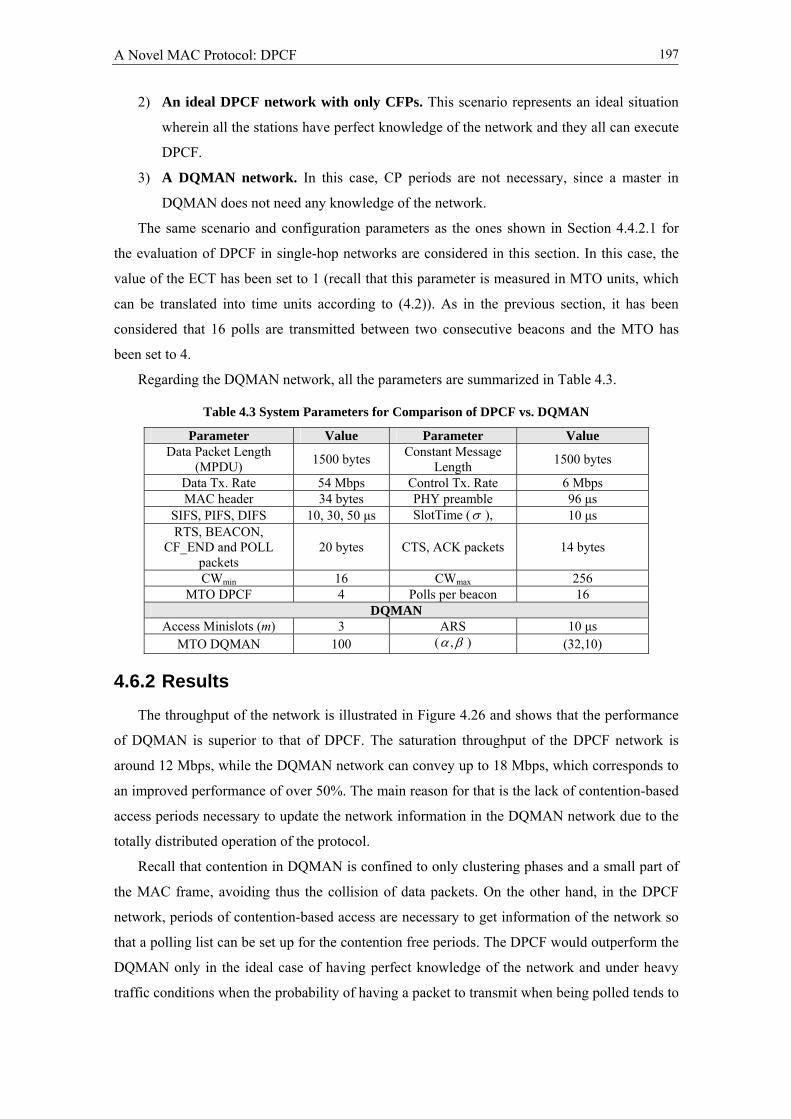
A Novel MAC Protocol: DPCF
197
2) An ideal DPCF network with only CFPs. This scenario represents an ideal situation
wherein all the stations have perfect knowledge of the network and they all can execute
DPCF.
3) A DQMAN network. In this case, CP periods are not necessary, since a master in
DQMAN does not need any knowledge of the network.
The same scenario and configuration parameters as the ones shown in Section 4.4.2.1 for
the evaluation of DPCF in single-hop networks are considered in this section. In this case, the
value of the ECT has been set to 1 (recall that this parameter is measured in MTO units, which
can be translated into time units according to (4.2)). As in the previous section, it has been
considered that 16 polls are transmitted between two consecutive beacons and the MTO has
been set to 4.
Regarding the DQMAN network, all the parameters are summarized in Table 4.3.
Table 4.3 System Parameters for Comparison of DPCF vs. DQMAN
Parameter Value Parameter Value Data Packet Length
(MPDU) 1500 bytes
Constant Message Length
1500 bytes
Data Tx. Rate 54 Mbps Control Tx. Rate 6 Mbps MAC header 34 bytes PHY preamble 96 μs
SIFS, PIFS, DIFS 10, 30, 50 μs SlotTime ( ), 10 μs RTS, BEACON,
CF_END and POLL packets
20 bytes CTS, ACK packets 14 bytes
CWmin 16 CWmax 256 MTO DPCF 4 Polls per beacon 16
DQMAN Access Minislots (m) 3 ARS 10 μs
MTO DQMAN 100 ( , ) (32,10)
4.6.2 Results
The throughput of the network is illustrated in Figure 4.26 and shows that the performance
of DQMAN is superior to that of DPCF. The saturation throughput of the DPCF network is
around 12 Mbps, while the DQMAN network can convey up to 18 Mbps, which corresponds to
an improved performance of over 50%. The main reason for that is the lack of contention-based
access periods necessary to update the network information in the DQMAN network due to the
totally distributed operation of the protocol.
Recall that contention in DQMAN is confined to only clustering phases and a small part of
the MAC frame, avoiding thus the collision of data packets. On the other hand, in the DPCF
network, periods of contention-based access are necessary to get information of the network so
that a polling list can be set up for the contention free periods. The DPCF would outperform the
DQMAN only in the ideal case of having perfect knowledge of the network and under heavy
traffic conditions when the probability of having a packet to transmit when being polled tends to
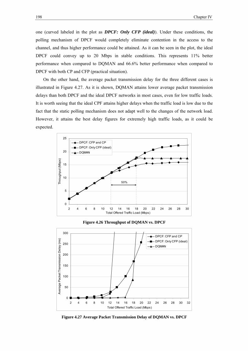
Chapter IV
198
one (curved labeled in the plot as DPCF: Only CFP (ideal)). Under these conditions, the
polling mechanism of DPCF would completely eliminate contention in the access to the
channel, and thus higher performance could be attained. As it can be seen in the plot, the ideal
DPCF could convey up to 20 Mbps in stable conditions. This represents 11% better
performance when compared to DQMAN and 66.6% better performance when compared to
DPCF with both CP and CFP (practical situation).
On the other hand, the average packet transmission delay for the three different cases is
illustrated in Figure 4.27. As it is shown, DQMAN attains lower average packet transmission
delays than both DPCF and the ideal DPCF networks in most cases, even for low traffic loads.
It is worth seeing that the ideal CPF attains higher delays when the traffic load is low due to the
fact that the static polling mechanism does not adapt well to the changes of the network load.
However, it attains the best delay figures for extremely high traffic loads, as it could be
expected.
0
5
10
15
20
25
2 4 6 8 10 12 14 16 18 20 22 24 26 28 30Total Offered Traffic Load (Mbps)
Th
rou
gh
pu
t (M
bp
s)
DPCF: CFP and CP
DPCF: Only CFP (ideal)
DQMAN
50%
Figure 4.26 Throughput of DQMAN vs. DPCF
0
50
100
150
200
250
300
2 4 6 8 10 12 14 16 18 20 22 24 26 28 30 32
Total Offered Traffic Load (Mbps)
Ave
rag
e P
ack
et T
ran
smis
sio
n D
ela
y (m
s)
DPCF: CFP and CP
DPCF: Only CFP (ideal)
DQMAN
Figure 4.27 Average Packet Transmission Delay of DQMAN vs. DPCF
A Novel MAC Protocol: DPCF
199
The main reason for the higher delay in both the DPCF and the ideal DPCF networks for
traffic loads below 18 Mbps is that, for the duration of a contention free period, a station with
data to transmit has to wait until it is polled in order to be able to transmit. On the other hand, in
the DQMAN network the access request can be sent as soon as there is a data packet to transmit
and there are no collisions pending to be solved. For this reason, the average packet
transmission delay in the DQMAN network is considerably reduced compared to that of the
DPCF network.
4.7 Chapter Conclusions
DPCF has been presented in this chapter as the extension of the point coordination function
(PCF) of the IEEE 802.11 Standard, designed for infrastructure-based networks, to operate over
distributed wireless ad hoc networks without infrastructure. The aim of this chapter is to expose
a simple case study that shows that the rationale presented in the context of DQMAN to extend
DQCA to ad hoc networks can be indeed applied to any other infrastructure-based MAC.
Performance evaluation of the protocol through link-level computer simulation shows that
the approach achieves the goal of improving the performance of ad hoc networks when
compared to current standards only based on random access. In addition, the results presented
show that the methodology used in the design of the protocol is very efficient in extending the
operation of PCF to be executed in networks without infrastructure.
As it was done in the previous chapter for DQMAN, a performance evaluation of a mixed
network wherein DPCF stations coexist with legacy DCF stations has been also presented.
Results show that the protocol is fully compatible with already deployed legacy standard-based
networks. Moreover, by properly selecting the value of a parameter named ECT, which
corresponds to the time that the stations are periodically forced to operate in DCF mode, the
performance of the network can be tuned at will. Actually, there is a tradeoff to be managed
between fairness among the different types of stations and the overall network performance.
Finally, and for the sake of completeness, a comparison of the performance of DQMAN and
DPCF has been also presented. Results show that DQMAN outperforms DPCF in all the cases
presented in this chapter. Moreover, DQMAN can be executed without any knowledge of the
network while when executing DPCF it is necessary to have some knowledge of the network in
order to execute the polling mechanism once a station is set to master mode. Note that whenever
a station is set to master mode, it requires a list of neighbors to poll. However, the main strength
of DPCF when compared to DQMAN is that it is strongly based on the IEEE 802.11 Standard,
and this facilitates its implementation in real off-the-shelf hardware.
The results presented in this chapter are rather promising and, in fact, future work will be
aimed at optimizing the design of the DPCF and at implementing the protocol in a real testbed
to evaluate its actual performance in a real environment.
Chapter IV
200
4.8 References
[1] IEEE, Part 11: Wireless LAN Medium Access Control (MAC) and Physical Layer
(PHY) Specifications, IEEE Std. 802.-11-99, Aug. 1999.
[2] IEEE Std. 802.11g, Supplement to Part 11: Wireless LAN Medium Access Control
(MAC) and Physical Layer (PHY) Specifications; Further High-Speed Physical Layer
Extension in the 2.4GHz Band, 2003.
201
Chapter V
5 Cooperative ARQ: DQCOOP and PRCSMA
5.1 Introduction
DQMAN has been presented in the first main part of this thesis as an innovative MAC
protocol for infrastructureless networks. The protocol performs at maximum efficiency when
the users of a network are naturally organized into groups, which inherently become clusters.
Even though DQMAN can be executed over sparsely distributed networks along multiple paths
with simultaneous active clusters, its maximum benefits can be obtained when the users
contending for the channel are somehow grouped. This is the case of most of the proposed
cooperative communication schemes [1].
As stated in the introductory section of Chapter I, according to visions of the Wireless
World Research Forum (WWRF), by the year 2017, “seven trillion wireless devices will be
serving seven billion people” [2]. Clearly, most of these devices will be for short-range
communication. One of the main consequences of these figures is that there will be always a
potential cooperative cluster (also referred to as wireless grid) surrounding any given wireless
device regardless of its specific location. In fact, this is a reasonable assumption even today. It
Chapter V
202
is possible to interconnect a personal laptop, a mobile phone, and a PDA to create a short-range
Personal Area Network (PAN). Therefore, around any wireless device, there might be a
potential group of helpers that can allow for the execution of different cooperative
communication schemes that may improve the efficiency of the communications. However,
involving a number of cooperative users in the communication requires coordination, at least in
order to avoid the waste of transmission resources. This is the main motivation of the last part of
the thesis.
More precisely, the focus in this part of the thesis is on Cooperative ARQ (C-ARQ)
schemes. By the time this thesis was started, the field of C-ARQ was a quite unknown research
topic. However, it is a very active research topic today. C-ARQ schemes constitute a practical
way of executing cooperation in wireless networks with already existing equipment and taking
into account the aforementioned market figures. C-ARQ schemes can be considered as a kind of
cooperative schemes that exploit feedback from the receiver. In C-ARQ, cooperation is only
requested when actually needed, and thus the efficiency of the network can be improved with
respect to other cooperative schemes. C-ARQ schemes can provide spatial diversity and attain
higher transmission rates, lower transmission delays, more efficient energy consumption, or
extended coverage, among other possibilities.
In short, the idea of C-ARQ is to exploit the broadcast nature of the wireless channel in the
following manner: any transmission can be received by not only the intended destination of the
transmission, but also by any of the stations in the transmission range of the transmitter. What
has been traditionally considered as interference, is exploited in C-ARQ schemes to attain
spatial diversity. Upon a transmission error, a retransmission can be requested from any (or
some) of the stations which overheard the original transmission, which can act as spontaneous
helpers (or relays). The result is that the destination of a packet can receive different copies of
the same information arriving via statistically independent transmission paths.
The rest of this section is organized as follows. A deeper incursion into the concept of C-
ARQ is presented in Section 5.1.1. The background of C-ARQ schemes, a formal description of
their operation, and a discussion of their performance in wireless networks is presented in that
section. Both the motivation and main contributions of this thesis regarding C-ARQ schemes
are presented in Section 5.1.2. The structure of the rest of the chapter is also presented in that
section. To conclude this introductory section, and for completeness, some related work is
overviewed in Section 5.1.3.
Cooperative ARQ: DQCOOP and PRCSMA 203
5.1.1 Cooperative ARQ (C-ARQ)
5.1.1.1 Background and Motivation
Traditionally, ARQ schemes have been used in communication networks to guarantee the
reliable delivery of data packets. Upon the reception of a packet with errors, retransmissions are
requested from the source until either the packet can be properly decoded or it is discarded for
the benefit of the backlogged data.
Error Detection (ED) information is usually attached to the data packets so that the intended
destination can learn whether a packet has been received with errors or not. Typically, this ED
information gets the form of a CRC attached to the overhead (either to the header or to the tail)
of data packets. In hybrid ARQ schemes, Forward Error Correction (FEC) information is also
attached to the overhead of the packets in order to reduce the probability of error occurrence.
According to the retransmitted information, ARQ schemes can be classified as:
1) Type I, if retransmissions are exact copies of the failed packet.
2) Type II, if there is incremental redundancy added to the retransmissions.
On the other hand, according to the acknowledgement and retransmission strategy, ARQ
schemes can be further classified into three main groups:
1) Stop and Wait ARQ (S&W), where no new packet can be transmitted until the correct
reception of the current packet is acknowledged by the intended destination.
Considering the relatively fast dynamics and variability of the radio channel, this is the
most practical approach in wireless networks.
2) Go-Back-N ARQ, where the acknowledgement and retransmission procedure is
performed in groups of N packets. In the case of retransmission, all the N packets are
retransmitted.
3) Selective Repeat ARQ, where the acknowledgement is performed in groups of N
packets, but retransmission is only executed for the packets that where received with
errors, instead of retransmitting the N packets as in Go-Back-N.
Several variations of ARQ schemes have been proposed in the past to improve the
performance of communications. These schemes perform well in wired networks where there is
no correlation between consecutive packet error probabilities, i.e., packet errors are random and
sparse. However, their performance in wireless networks is compromised by phenomena such
as the shadowing and fading of the radio channel. In wireless channels, packet errors might
come into bursts, and thus if a packet is received with errors, the immediate retransmissions will
be also received with errors with high probability if they are performed through the same
channel [3], [4].
Only as an example, consider a wireless network operating at 2.4GHz over a Rayleigh
channel. fm is the maximum Doppler frequency which depends on the average speed (v) of the
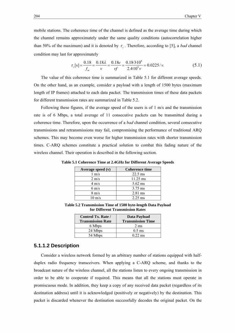
Chapter V
204
mobile stations. The coherence time of the channel is defined as the average time during which
the channel remains approximately under the same quality conditions (autocorrelation higher
than 50% of the maximum) and it is denoted by c . Therefore, according to [5], a bad channel
condition may last for approximately
8
9
0.18 0.18 0.18 0.18·3·10[s] 0.0225/ .
2.4·10cm
cv
f v vf v
(5.1)
The value of this coherence time is summarized in Table 5.1 for different average speeds.
On the other hand, as an example, consider a payload with a length of 1500 bytes (maximum
length of IP frames) attached to each data packet. The transmission times of these data packets
for different transmission rates are summarized in Table 5.2.
Following these figures, if the average speed of the users is of 1 m/s and the transmission
rate is of 6 Mbps, a total average of 11 consecutive packets can be transmitted during a
coherence time. Therefore, upon the occurrence of a bad channel condition, several consecutive
transmissions and retransmissions may fail, compromising the performance of traditional ARQ
schemes. This may become even worse for higher transmission rates with shorter transmission
times. C-ARQ schemes constitute a practical solution to combat this fading nature of the
wireless channel. Their operation is described in the following section.
Table 5.1 Coherence Time at 2.4GHz for Different Average Speeds
Average speed (v) Coherence time 1 m/s 22.5 ms 2 m/s 11.25 ms 4 m/s 5.62 ms 6 m/s 3.75 ms 8 m/s 2.81 ms
10 m/s 2.25 ms
Table 5.2 Transmission Time of 1500 byte-length Data Payload for Different Transmission Rates
Control Tx. Rate / Transmission Rate
Data Payload Transmission Time
6 Mbps 2 ms 24 Mbps 0.5 ms 54 Mbps 0.22 ms
5.1.1.2 Description
Consider a wireless network formed by an arbitrary number of stations equipped with half-
duplex radio frequency transceivers. When applying a C-ARQ scheme, and thanks to the
broadcast nature of the wireless channel, all the stations listen to every ongoing transmission in
order to be able to cooperate if required. This means that all the stations must operate in
promiscuous mode. In addition, they keep a copy of any received data packet (regardless of its
destination address) until it is acknowledged (positively or negatively) by the destination. This
packet is discarded whenever the destination successfully decodes the original packet. On the
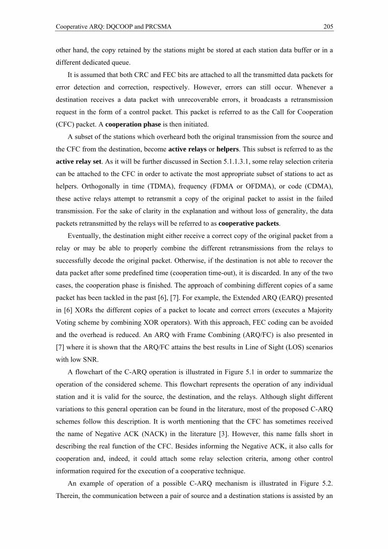
Cooperative ARQ: DQCOOP and PRCSMA 205
other hand, the copy retained by the stations might be stored at each station data buffer or in a
different dedicated queue.
It is assumed that both CRC and FEC bits are attached to all the transmitted data packets for
error detection and correction, respectively. However, errors can still occur. Whenever a
destination receives a data packet with unrecoverable errors, it broadcasts a retransmission
request in the form of a control packet. This packet is referred to as the Call for Cooperation
(CFC) packet. A cooperation phase is then initiated.
A subset of the stations which overheard both the original transmission from the source and
the CFC from the destination, become active relays or helpers. This subset is referred to as the
active relay set. As it will be further discussed in Section 5.1.1.3.1, some relay selection criteria
can be attached to the CFC in order to activate the most appropriate subset of stations to act as
helpers. Orthogonally in time (TDMA), frequency (FDMA or OFDMA), or code (CDMA),
these active relays attempt to retransmit a copy of the original packet to assist in the failed
transmission. For the sake of clarity in the explanation and without loss of generality, the data
packets retransmitted by the relays will be referred to as cooperative packets.
Eventually, the destination might either receive a correct copy of the original packet from a
relay or may be able to properly combine the different retransmissions from the relays to
successfully decode the original packet. Otherwise, if the destination is not able to recover the
data packet after some predefined time (cooperation time-out), it is discarded. In any of the two
cases, the cooperation phase is finished. The approach of combining different copies of a same
packet has been tackled in the past [6], [7]. For example, the Extended ARQ (EARQ) presented
in [6] XORs the different copies of a packet to locate and correct errors (executes a Majority
Voting scheme by combining XOR operators). With this approach, FEC coding can be avoided
and the overhead is reduced. An ARQ with Frame Combining (ARQ/FC) is also presented in
[7] where it is shown that the ARQ/FC attains the best results in Line of Sight (LOS) scenarios
with low SNR.
A flowchart of the C-ARQ operation is illustrated in Figure 5.1 in order to summarize the
operation of the considered scheme. This flowchart represents the operation of any individual
station and it is valid for the source, the destination, and the relays. Although slight different
variations to this general operation can be found in the literature, most of the proposed C-ARQ
schemes follow this description. It is worth mentioning that the CFC has sometimes received
the name of Negative ACK (NACK) in the literature [3]. However, this name falls short in
describing the real function of the CFC. Besides informing the Negative ACK, it also calls for
cooperation and, indeed, it could attach some relay selection criteria, among other control
information required for the execution of a cooperative technique.
An example of operation of a possible C-ARQ mechanism is illustrated in Figure 5.2.
Therein, the communication between a pair of source and a destination stations is assisted by an
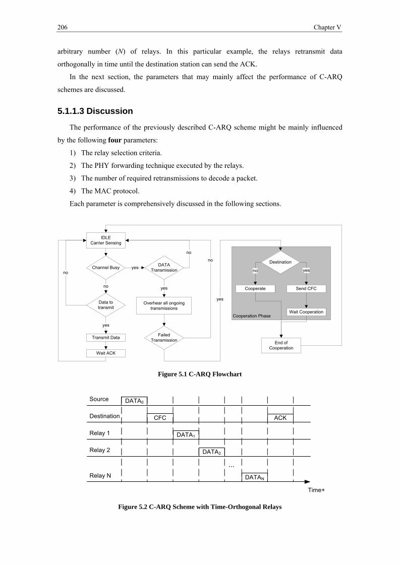
Chapter V
206
arbitrary number (N) of relays. In this particular example, the relays retransmit data
orthogonally in time until the destination station can send the ACK.
In the next section, the parameters that may mainly affect the performance of C-ARQ
schemes are discussed.
5.1.1.3 Discussion
The performance of the previously described C-ARQ scheme might be mainly influenced
by the following four parameters:
1) The relay selection criteria.
2) The PHY forwarding technique executed by the relays.
3) The number of required retransmissions to decode a packet.
4) The MAC protocol.
Each parameter is comprehensively discussed in the following sections.
Cooperation Phase
IDLECarrier Sensing
Data to transmit
Channel Busy
no
DATA Transmission
yes
no
Overhear all ongoing transmissions
yes
no
Transmit Data
yes
Failed Transmission
Wait ACK
no Destination
yes
Send CFCCooperate
yesno
Wait Cooperation
End of Cooperation
Figure 5.1 C-ARQ Flowchart
Source
Destination
Relay 1
Relay 2
DATA0
CFC
DATA1
DATA2
ACK
Relay N DATAN
Time+
...
Figure 5.2 C-ARQ Scheme with Time-Orthogonal Relays
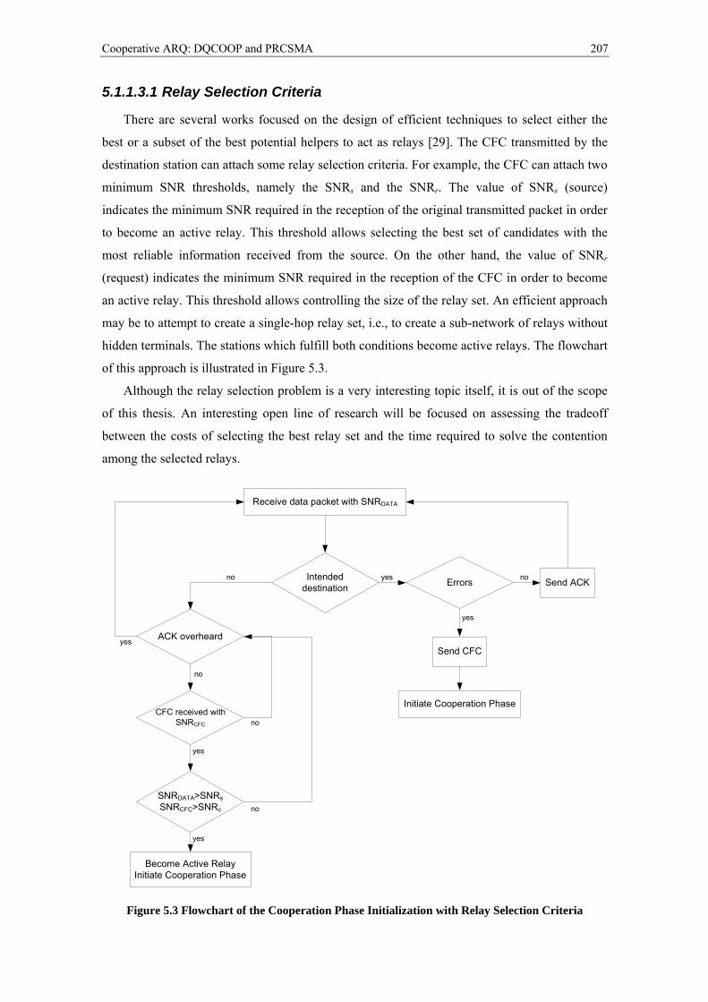
Cooperative ARQ: DQCOOP and PRCSMA 207
5.1.1.3.1 Relay Selection Criteria
There are several works focused on the design of efficient techniques to select either the
best or a subset of the best potential helpers to act as relays [29]. The CFC transmitted by the
destination station can attach some relay selection criteria. For example, the CFC can attach two
minimum SNR thresholds, namely the SNRs and the SNRr. The value of SNRs (source)
indicates the minimum SNR required in the reception of the original transmitted packet in order
to become an active relay. This threshold allows selecting the best set of candidates with the
most reliable information received from the source. On the other hand, the value of SNRr
(request) indicates the minimum SNR required in the reception of the CFC in order to become
an active relay. This threshold allows controlling the size of the relay set. An efficient approach
may be to attempt to create a single-hop relay set, i.e., to create a sub-network of relays without
hidden terminals. The stations which fulfill both conditions become active relays. The flowchart
of this approach is illustrated in Figure 5.3.
Although the relay selection problem is a very interesting topic itself, it is out of the scope
of this thesis. An interesting open line of research will be focused on assessing the tradeoff
between the costs of selecting the best relay set and the time required to solve the contention
among the selected relays.
SNRDATA>SNRs
SNRCFC>SNRc
Receive data packet with SNRDATA
Become Active RelayInitiate Cooperation Phase
Intendeddestination
ACK overheard
Errors Send ACK
Send CFC
CFC received with SNRCFC
Initiate Cooperation Phase
yesno
no
no
no
no
yes
yes
yes
yes
Figure 5.3 Flowchart of the Cooperation Phase Initialization with Relay Selection Criteria
Chapter V
208
5.1.1.3.2 PHY Forwarding Technique
According to the specific strategy applied by the relays it is possible to classify cooperative
(relay) techniques as:
a) Amplify and forward techniques, when the relays transmit an amplified version of the
original received signal, without demodulating or decoding it.
b) Compress and forward techniques, when the relays transmit a compressed version of
the original transmitted signal, without decoding it.
c) Decode and forward techniques, when the relays transmit recoded copies of the original
message. Note that using decode and forward, the recoding process can be done on the
basis of repeating the original codification, recoding the original data (or only a relevant
part of it), or using more sophisticated Space-Time Codes (STC) [13].
The design of cooperative schemes at the PHY layer constitutes an intense area of research.
Nevertheless, the focus of this thesis is on cooperative techniques at the Data Link Control layer
and, as a matter of fact, the ideas presented in this work could work on top of any PHY layer
and cooperative PHY mechanism, and thus on top of any cooperation architecture.
5.1.1.3.3 Number of Retransmissions
The average number of cooperative retransmissions required to successfully decode a
packet initially received with errors depends on many factors. They can be mainly classified
into two groups depending on:
a) The channel conditions between the source and the destination, the source and the
relays, and the relays and the destination.
b) The transmission scheme, which includes the forwarding technique executed by the
relays and the combination technique executed by the destination station to combine the
different retransmissions received from independent paths.
For example, it is shown in [10] that the reception of retransmissions from the relays can be
seen as a virtual increase in the total SNR perceived at destination. In that paper, authors
consider a scenario formed by a source, a destination, and a fixed number of relays. It is
assumed that retransmissions from the relays to the destination are error-free. They focus their
work on the low-SNR regime and they approximate the equivalent data transmission rate from
the source to the destination (RMRC) of a variation of Decode and Forward C-ARQ scheme (the
relays can retransmit regardless of whether they have received the original transmission from
the source with or without errors) with a Maximum Ratio Combiner at destination and
considering a Rayleigh channel by
1
2
1 3log 1 ,
2 2
K
MRC e
KR b p
K
(5.2)
Cooperative ARQ: DQCOOP and PRCSMA 209
where:
K is the number of retransmissions.
b is the number of bits per symbol (modulation).
pe is the target packet error probability.
is the average received SNR from the source.
With (5.2) and given a data transmission rate, it is possible to compute the average number
of retransmissions K needed to decode a packet with probability pe.
Another example can be found in [11] where it is shown that due to impartial channel
knowledge, for example due to high mobility, the number of required retransmissions in an
ARQ scheme can be determined resorting to curves or either analytical approximations.
5.1.1.3.4 MAC Protocol
A MAC protocol is necessary to tackle with the contention among the relays. Just as an
example, the ideal scheduling among the relays represented in Figure 5.2 is impossible to attain
in fully distributed networks without a central coordinator. Therefore, the set of active relays
should contend for the channel in order to retransmit the packets. Efficient MAC protocols are
necessary to execute a C-ARQ scheme in order to exploit the benefits of cooperation in wireless
networks. Indeed, this is the main motivation of the contribution presented in this part of the
thesis.
5.1.2 Motivation and Contributions of the Chapter
C-ARQ schemes have been so far analyzed from a fundamental point of view and mainly
with emphasis on the PHY layer [3], [14]-[18]. Most of these works consider simplified
network topologies and ideal TDMA scheduling among the relays at the MAC level. More
precisely, the gain of a C-ARQ scheme in terms of improved probability of error is discussed in
[3]. In [14], the SNR equivalent gain and the average number of required retransmissions of a
single source cooperative ARQ protocol are studied. In [15] the performance of different
cooperative schemes is derived in terms of outage probability and SNR gain, while in [16] the
saturation throughput of three double-source cooperative ARQ protocols is presented. Cerutti et
al. present in [17] a model to evaluate data delay for single-source and single-relay cooperative
ARQ protocols. In [18], Morillo et al. propose a Collaborative ARQ (also referred to as C-
ARQ) protocol that exploits diversity through collaboration in wireless networks. They
demonstrate that when M neighboring stations collaborate using the proposed algorithm they
can get the same efficiency as an array of M antennas.
Some other works have been focused on the relay selection criteria within the context of C-
ARQ schemes. For example, in the works presented in [19] and [20], an opportunistic
forwarding scheme is presented wherein the best candidate to retransmit is selected whenever a
Chapter V
210
communication has failed. On the other hand, a scenario wherein a set of the best candidates is
selected is discussed in [21], therein referred to as cloud of relays.
Previous work has put in evidence that C-ARQ schemes may yield an improvement in
performance, lower energy consumption, and interference, as well as an extended coverage area
by allowing communication at low SNRs. However, as aforementioned, all of these
contributions assume simplified topologies and perfect scheduling among the relays at the MAC
level. This scheduling might be difficult to attain in the fully decentralized scenario represented
by the cloud or relays, i.e., the active relay set, without infrastructure. Therefore, the design of
efficient MAC protocols is mandatory if C-ARQ schemes are to find real application, as well as
the evaluation of the actual performance of these techniques (considering the MAC overhead).
Indeed, this is the main motivation for the contribution presented in this chapter of the thesis.
In particular, the focus in this thesis is on time-orthogonal C-ARQ schemes, which might
be the most feasible implementation with already existing off-the-shelf equipment. By slightly
modifying the wireless controller (or driver), existing wireless cards could implement a C-ARQ
scheme. The emphasis is on the design and analysis of novel MAC protocols to deal with the
unique characteristics of the contention process that takes place among the active relays within a
cooperation phase. Note that in the considered C-ARQ schemes, upon the initialization of the
cooperation phase, the network has the three following unique characteristics:
1) The spontaneous “sub-network” formed by the active relays is ad hoc and thus there is
no infrastructure responsible for managing the access to the channel.
2) This sub-network formed by the active relays surrounding the node calling for
cooperation is suddenly (sharply) set into saturation conditions whenever the
cooperation phase is initiated. Upon the transmission of a CFC packet, all the active
relays have a data packet ready to transmit in order to assist the failed transmission.
Therefore, heavy contention comes up in a previously idle network.
3) Opposite to general communications systems, now fairness is not a major issue to
achieve. Indeed, the main goal is to attempt to assist the failed transmission as fast and
reliable as possible, minimizing the use of the radio resources.
These three characteristics determine the way MAC protocols should be designed within the
context of C-ARQ schemes in wireless networks. Considering the aforementioned
characteristics, the main contributions of the thesis regarding this issue are:
1) The design and analysis of an adaptation of the DQMAN protocol for C-ARQ schemes,
named DQCOOP, presented in Section 5.2.
2) The design and analysis of the Persistent Relay CSMA (PRCSMA) protocol, presented
in Section 5.3. It is an 802.11-based MAC protocol for the execution of C-ARQ
schemes in general wireless networks. This protocol is backwards compatible and can
be considered as a benchmark reference for comparison purposes.
Cooperative ARQ: DQCOOP and PRCSMA 211
3) The comprehensive comparison between the performances of the two protocols,
presented in Section 5.4. Both protocols are also compared to an ideal perfect
scheduling system. This comparison explicitly evaluates the overhead generated by an
actual MAC protocol, and demonstrates that its effect must not be neglected in order to
evaluate the real performance of any C-ARQ scheme.
4) As a case study, the analysis of the overall performance of a rooftop infrastructure-
based scenario with the execution of a C-ARQ scheme, considering both DQCOOP and
PRCSMA. This analysis is presented in Section 5.5. Rooftop scenarios represent a wide
range of real networks, and this is the main reason to focus our research on this kind of
scenarios.
It is worth mentioning at this point that, in the literature, there exists a family of cooperative
MAC protocols [22]-[28] which have not been designed for the execution of C-ARQ schemes in
wireless networks, but they are aimed at solving other kind of interesting cooperative issues. For
completeness, they are overviewed in the following section.
5.1.3 Related work: Cooperative MAC Protocols
Some MAC protocols for cooperative communications have been proposed in the literature.
Most of them have been designed to achieve a throughput enhancement, but actually none of
them takes into account all of the unique characteristics of the on-demand C-ARQ schemes. It
has to be mentioned that all these MAC protocols have been designed more as routing protocols
with a cross-layer design that takes into account the transmission rates to decide the shortest
route to a destination than as MAC protocols themselves. In what follows, a summary of the
most relevant contributions is summarized.
In [22] two versions of the CoopMAC protocol are designed in the context of 802.11b
WLANs in order to solve the performance anomaly induced by the multi-rate capability of the
DCF of the standard [9]. Users with low transmission rate occupy the channel during longer
periods of time, reducing the overall throughput of the system and reducing the throughput seen
by stations with higher transmission rates. The main idea of CoopMAC protocols is that stations
transmit first to intermediate stations at a higher rate and then those intermediate stations
transmit to the access point, reducing the total transmission delay. In the first version of
CoopMAC, referred to as CoopMAC I, any station keeps updated a table with those stations
that could potentially help in a transmission. Before transmitting any packet, a station calculates
the shorter transmission path, either using direct communication with the intended destination
or through any of the potential helpers with an entry in the table. In the case of using any relay,
a previous handshake is done between the source station and the elected relay in order to ensure
the validity of the route. The main drawback of CoopMAC I is that it requires the addition of
three new fields in the Request To Send (RTS) frame and the addition of a new control frame
Chapter V
212
named Helper ready To Send (HTS). As an alternative, CoopMAC II is proposed to overcome
this problem. This second version of CoopMAC uses available empty fields in regular IEEE
802.11 control frames and eliminates the handshake between destination and helpers. Although
the implementation is simpler, version II is more vulnerable to a change in the availability of a
helping station caused by mobility. Computer simulations in [22] demonstrate the improved
performance achieved with either CoopMAC I or II. Moreover, Korakis et al. implemented the
protocol in actual WLAN cards, as reported in [23]. The main contribution in [23] is the
description of the overall implementation process and the limitations found when attempting to
actually implement the protocol. These limitations were mainly due to the constraints imposed
by the time sensitive tasks performed by the firmware of the wireless cards. In addition, the
CoopMAC has been also adapted to wireless networks using directional antennas in [24].
On the other hand, both the Cooperative-MAC (CMAC) and FEC CMAC (FCMAC)
protocols were presented in [25] within the context of 802.11e networks to improve the overall
performance and to ensure a certain QoS. In CMAC, a station detecting an erroneous packet
transmission between any other pair of source-destination station decides to cooperate by
retransmitting a copy of the overheard transmission as long as the received packet has no errors.
A random backoff mechanism with a constant backoff window is applied to avoid collisions
among different helpers. The size of the contention window of the helpers has to be very small
in comparison to the contention window of the source in order to ensure that helpers retransmit
their copy before the original source retransmits on its own the failed packet. Each helper
transmits at most once the copy of the packet to ensure that all available helpers cooperate and
thus the benefits of diversity are obtained. On the other hand, FCMAC extends the operation of
CMAC by fragmenting data packets into smaller blocks. Each block contains its own inner FEC
field and the whole packet contains an outer FEC. Upon error detection of a whole packet, only
a predefined number of randomly selected blocks among those received without errors are
retransmitted. If the retransmitted blocks are those that were received with errors at destination,
then the performance is improved. Otherwise, the increased overhead becomes useless. A
possible solution consists in adding a negative acknowledgement (NACK) sent out by the
destination upon error detection, indicating which are the blocks received with errors. However,
the use of NACK in CMAC would imply higher overhead and again, it would require hardware
modifications, thus breaking with the claimed backwards compatibility. The main limitation of
CMAC and FCMAC is that they rely on the fact that helpers can learn whether other
transmission between any pair of source and destination are successful or not only by
overhearing the radio channel.
In [26], the Cooperative Diversity Medium Access with Collision Avoidance (CD-MACA)
protocol is proposed within the context of wireless ad hoc networks operating over the
CSMA/CA protocol. Whenever a source terminal fails to receive the CTS packet, all those
Cooperative ARQ: DQCOOP and PRCSMA 213
stations that had properly received it, take the place of the source terminal and retransmit the
data packet. An analytical model based on Markov chain theory is proposed to obtain the
achievable throughput of the system considering cooperation. Although the general idea of CD-
MACA is rather interesting, the definition in [26] is quite general and several implementation
details are not considered.
From an energy-efficient perspective, another cooperative MAC protocol is also presented
within the context of ad hoc networks in [27]. This proposal integrates cooperative diversity
into two different wireless routing protocols by embedding a distributed cooperative MAC. The
initial path establishment performed by the routing protocol can be done either considering
cooperation or not. Cooperation is then achieved by making all stations act as a distributed
virtual antenna, by which simultaneous transmissions are separated through CDMA.
In [28] a cooperative MAC protocol was presented within the context of a mesh network
formed by an access point, a number of regular stations, and one fixed wireless router (relay). A
fixed TDMA scheme is applied and empty slots are used for cooperative relaying. The relay
station keeps a copy of all those packets that are not properly received by the AP. At the
beginning of each time slot, the relay listens to the channel. If the channel is idle, it retransmits
the packet at the head of its queue. Based on this main idea, in [28], two specific algorithms are
proposed to exploit the benefits of cross-layer design between the PHY and MAC layers.
The aforementioned, MAC protocols have been designed to achieve an improvement in the
network performance by transmitting through faster multi-hop routes. However, none of them
takes into account the unique characteristics of the C-ARQ schemes for their implementation in
on-demand cooperative schemes. DQCOOP is presented in the next section as a novel MAC
protocol that has been tailored to meet the requirements of the C-ARQ scenario. It constitutes
the adaptation of DQMAN to this kind of scenarios.
5.2 DQMAN for C-ARQ: DQCOOP
The aim of this section is to extend and adapt DQMAN to match the unique requirements
posed by the C-ARQ schemes. The new resultant protocol is called DQCOOP.
For clarity of explanation, it is assumed hereafter that the reader is already familiar with
both the operation and nomenclature of DQMAN presented in Chapter III of this thesis, and
with the C-ARQ scheme defined in the previous section.
5.2.1 Introduction and Problem Statement
The intuitive idea behind DQCOOP is that the destination asking for cooperation gets the
role of master and coordinates the retransmissions from the relays, which become its slaves.
This is represented in Figure 5.4.
The master, i.e., the destination, initiates the periodic broadcast of FBP and creates a
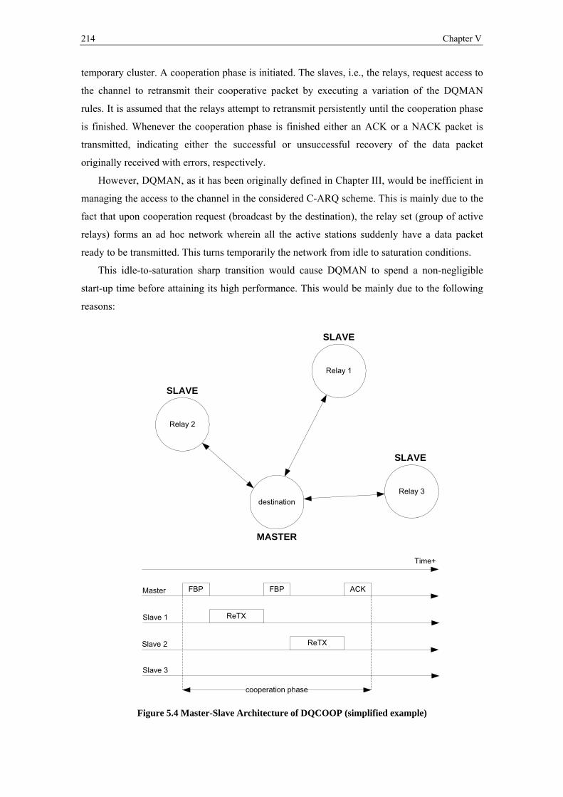
Chapter V
214
temporary cluster. A cooperation phase is initiated. The slaves, i.e., the relays, request access to
the channel to retransmit their cooperative packet by executing a variation of the DQMAN
rules. It is assumed that the relays attempt to retransmit persistently until the cooperation phase
is finished. Whenever the cooperation phase is finished either an ACK or a NACK packet is
transmitted, indicating either the successful or unsuccessful recovery of the data packet
originally received with errors, respectively.
However, DQMAN, as it has been originally defined in Chapter III, would be inefficient in
managing the access to the channel in the considered C-ARQ scheme. This is mainly due to the
fact that upon cooperation request (broadcast by the destination), the relay set (group of active
relays) forms an ad hoc network wherein all the active stations suddenly have a data packet
ready to be transmitted. This turns temporarily the network from idle to saturation conditions.
This idle-to-saturation sharp transition would cause DQMAN to spend a non-negligible
start-up time before attaining its high performance. This would be mainly due to the following
reasons:
destination
Relay 1
Relay 2
Relay 3
SLAVE
SLAVE
SLAVE
MASTER
Time+
Master
Slave 1
Slave 2
Slave 3
FBP
ReTX
FBP
ReTX
ACK
cooperation phase
Figure 5.4 Master-Slave Architecture of DQCOOP (simplified example)
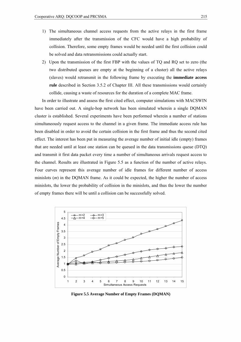
Cooperative ARQ: DQCOOP and PRCSMA 215
1) The simultaneous channel access requests from the active relays in the first frame
immediately after the transmission of the CFC would have a high probability of
collision. Therefore, some empty frames would be needed until the first collision could
be solved and data retransmissions could actually start.
2) Upon the transmission of the first FBP with the values of TQ and RQ set to zero (the
two distributed queues are empty at the beginning of a cluster) all the active relays
(slaves) would retransmit in the following frame by executing the immediate access
rule described in Section 3.5.2 of Chapter III. All these transmissions would certainly
collide, causing a waste of resources for the duration of a complete MAC frame.
In order to illustrate and assess the first cited effect, computer simulations with MACSWIN
have been carried out. A single-hop network has been simulated wherein a single DQMAN
cluster is established. Several experiments have been performed wherein a number of stations
simultaneously request access to the channel in a given frame. The immediate access rule has
been disabled in order to avoid the certain collision in the first frame and thus the second cited
effect. The interest has been put in measuring the average number of initial idle (empty) frames
that are needed until at least one station can be queued in the data transmissions queue (DTQ)
and transmit it first data packet every time a number of simultaneous arrivals request access to
the channel. Results are illustrated in Figure 5.5 as a function of the number of active relays.
Four curves represent this average number of idle frames for different number of access
minislots (m) in the DQMAN frame. As it could be expected, the higher the number of access
minislots, the lower the probability of collision in the minislots, and thus the lower the number
of empty frames there will be until a collision can be successfully solved.
0
0.5
1
1.5
2
2.5
3
3.5
4
4.5
5
1 2 3 4 5 6 7 8 9 10 11 12 13 14 15Simultaneous Access Requests
Ave
rag
e N
um
be
r o
f Em
pty
Fra
me
s
m=2 m=3m=4 m=5
Figure 5.5 Average Number of Empty Frames (DQMAN)
Chapter V
216
In addition to the effects of the idle-to-saturation sharp transition upon cooperation request,
it is shown in Figure 5.5 that there is always at least one frame empty irrespective of the number
of simultaneous arrivals in the first frame, even for only one arrival when the probability of
collision is zero. This is due to the fact that the access minislots are placed at the beginning of
the MAC frame while the FBP is transmitted at the end of the frame. Therefore, by implicit
operation of the protocol, one frame is lost in every cooperation phase as long as the immediate
access rule is disabled or there is more than one active relay. Note that in the case of having a
single relay, by enabling the immediate access rule, no frames would be lost.
In summary, upon a cooperation request, three effects must be taken into consideration in
order to adapt the operation of DQMAN to be executed in a C-ARQ scheme:
1) At least one frame would be lost in a collision if the immediate access rule of DQMAN
is kept active and there is more than one active relay.
2) Even with this rule disabled, an empty frame would be present when the collision
resolution process starts due to the MAC frame structure with the feedback broadcast at
the end of the frame.
3) More than one frame would be empty at the beginning of the cooperation phase,
especially if the number of relays is high, due to the heavy contention period that arises
when all the relays request access to the channel simultaneously.
Therefore, it is necessary to expand and adapt the DQMAN operation to take into
consideration the aforementioned issues that may potentially degrade its performance in C-ARQ
schemes. DQCOOP is presented in the next section with the goal of attaining the near-optimum
performance of DQMAN within the context of the considered C-ARQ scheme.
The rest of this section is organized as follows. DQCOOP is presented in Section 5.2.2.
Rather than presenting a comprehensive description, it is assumed that the reader is already
familiar with DQMAN and the focus is on the modifications on both the clustering and the
MAC protocols. An operational example of DQCOOP is presented in Section 5.2.3 in order to
help in the understanding of the overall protocol operation. The average cooperation delay of
DQCOOP is analyzed in Section 5.2.4. The accuracy of the model is assessed in Section 5.2.5
by means of computer simulations and a performance evaluation of the protocol is also
presented. Section 5.2.6 concludes the section and gives some final remarks.
5.2.2 Protocol Description
The core operation of DQCOOP is highly based on DQMAN. However, the clustering
algorithm and the MAC protocol (frame structure and protocol rules) are modified to meet the
requirements of the C-ARQ scheme. Their descriptions are presented in the next two sections.
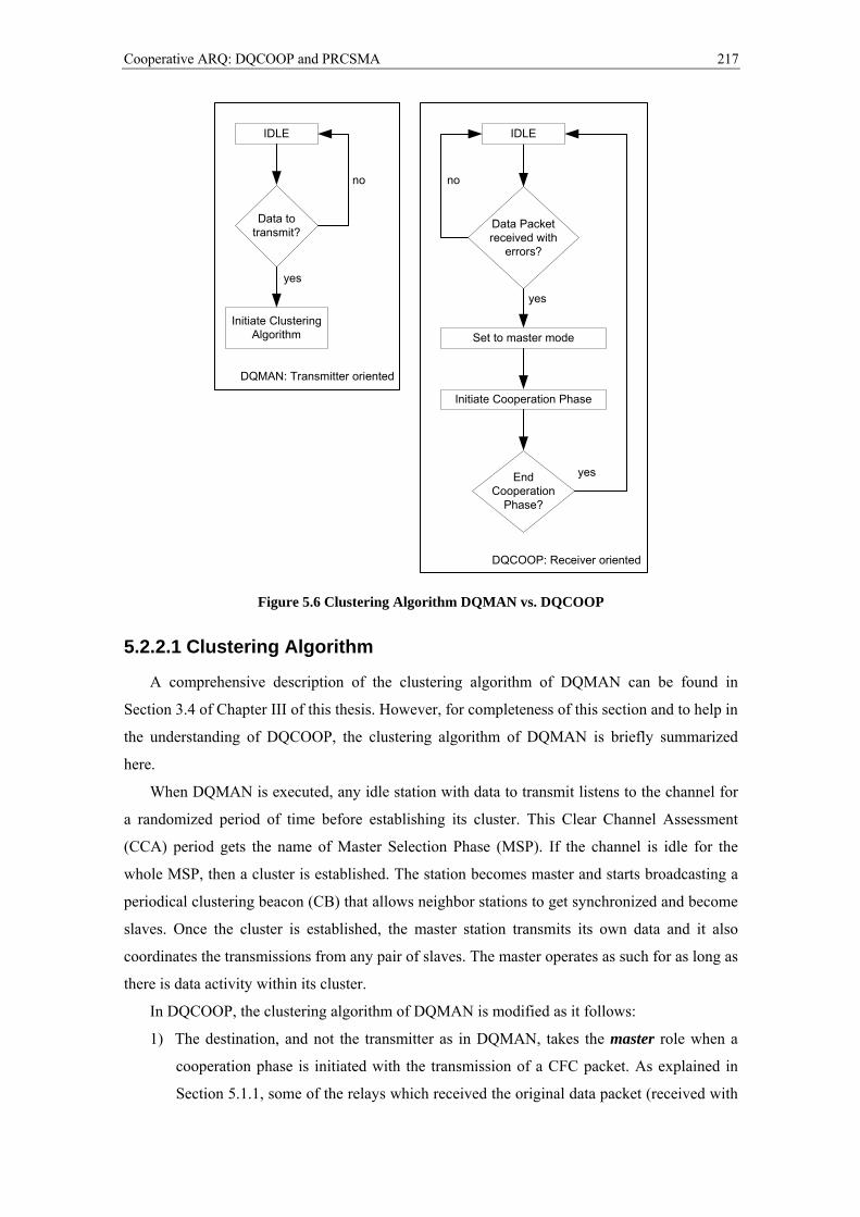
Cooperative ARQ: DQCOOP and PRCSMA 217
IDLE
Data to transmit?
Initiate Cooperation Phase
Data Packet received with
errors?
Initiate Clustering Algorithm Set to master mode
DQMAN: Transmitter oriented
DQCOOP: Receiver oriented
End Cooperation
Phase?
IDLE
no
yes
yes
no
yes
Figure 5.6 Clustering Algorithm DQMAN vs. DQCOOP
5.2.2.1 Clustering Algorithm
A comprehensive description of the clustering algorithm of DQMAN can be found in
Section 3.4 of Chapter III of this thesis. However, for completeness of this section and to help in
the understanding of DQCOOP, the clustering algorithm of DQMAN is briefly summarized
here.
When DQMAN is executed, any idle station with data to transmit listens to the channel for
a randomized period of time before establishing its cluster. This Clear Channel Assessment
(CCA) period gets the name of Master Selection Phase (MSP). If the channel is idle for the
whole MSP, then a cluster is established. The station becomes master and starts broadcasting a
periodical clustering beacon (CB) that allows neighbor stations to get synchronized and become
slaves. Once the cluster is established, the master station transmits its own data and it also
coordinates the transmissions from any pair of slaves. The master operates as such for as long as
there is data activity within its cluster.
In DQCOOP, the clustering algorithm of DQMAN is modified as it follows:
1) The destination, and not the transmitter as in DQMAN, takes the master role when a
cooperation phase is initiated with the transmission of a CFC packet. As explained in
Section 5.1.1, some of the relays which received the original data packet (received with
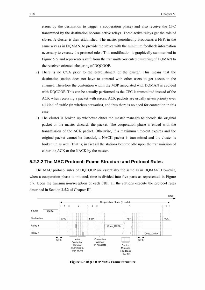
Chapter V
218
errors by the destination to trigger a cooperation phase) and also receive the CFC
transmitted by the destination become active relays. These active relays get the role of
slaves. A cluster is then established. The master periodically broadcasts a FBP, in the
same way as in DQMAN, to provide the slaves with the minimum feedback information
necessary to execute the protocol rules. This modification is graphically summarized in
Figure 5.6, and represents a shift from the transmitter-oriented clustering of DQMAN to
the receiver-oriented clustering of DQCOOP.
2) There is no CCA prior to the establishment of the cluster. This means that the
destination station does not have to contend with other users to get access to the
channel. Therefore the contention within the MSP associated with DQMAN is avoided
with DQCOOP. This can be actually performed as the CFC is transmitted instead of the
ACK when receiving a packet with errors. ACK packets are usually given priority over
all kind of traffic (in wireless networks), and thus there is no need for contention in this
case.
3) The cluster is broken up whenever either the master manages to decode the original
packet or the master discards the packet. The cooperation phase is ended with the
transmission of the ACK packet. Otherwise, if a maximum time-out expires and the
original packet cannot be decoded, a NACK packet is transmitted and the cluster is
broken up as well. That is, in fact all the stations become idle upon the transmission of
either the ACK or the NACK by the master.
5.2.2.2 The MAC Protocol: Frame Structure and Protocol Rules
The MAC protocol rules of DQCOOP are essentially the same as in DQMAN. However,
when a cooperation phase is initiated, time is divided into five parts as represented in Figure
5.7. Upon the transmission/reception of each FBP, all the stations execute the protocol rules
described in Section 3.5.2 of Chapter III.
Coop_DATA
FBP
SIFS
Time+
Contention Window
m minislots Control MinislotsFeedback
(S,C,E)
CFC
Coop_DATA
ACK
Cooperation Phase (5 parts)
FBP
Initial Contention
Windowm0 minislots,with m0>m
Relay 1
Source DATA
Destination
1 2 3 4 5
Relay n
SIFS
Figure 5.7 DQCOOP MAC Frame Structure
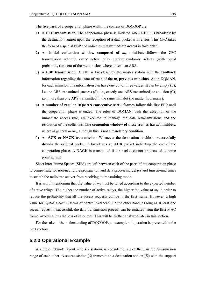
Cooperative ARQ: DQCOOP and PRCSMA 219
The five parts of a cooperation phase within the context of DQCOOP are:
1) A CFC transmission. The cooperation phase is initiated when a CFC is broadcast by
the destination station upon the reception of a data packet with errors. This CFC takes
the form of a special FBP and indicates that immediate access is forbidden.
2) An initial contention window composed of m0 minislots follows the CFC
transmission wherein every active relay station randomly selects (with equal
probability) one out of the m0 minislots where to send an ARS.
3) A FBP transmission. A FBP is broadcast by the master station with the feedback
information regarding the state of each of the m0 previous minislots. As in DQMAN,
for each minislot, this information can have one out of three values. It can be empty (E),
i.e., no ARS transmitted, success (S), i.e., exactly one ARS transmitted, or collision (C),
i.e., more than one ARS transmitted in the same minislot (no matter how many).
4) A number of regular DQMAN consecutive MAC frames follow this first FBP until
the cooperation phase is ended. The rules of DQMAN, with the exception of the
immediate access rule, are executed to manage the data retransmissions and the
resolution of the collisions. The contention window of these frames has m minislots,
where in general m<m0, although this is not a mandatory condition.
5) An ACK or NACK transmission. Whenever the destination is able to successfully
decode the original packet, it broadcasts an ACK packet indicating the end of the
cooperation phase. A NACK is transmitted if the packet cannot be decoded at some
point in time.
Short Inter Frame Spaces (SIFS) are left between each of the parts of the cooperation phase
to compensate for non-negligible propagation and data processing delays and turn around times
to switch the radio transceiver from receiving to transmitting mode.
It is worth mentioning that the value of m0 must be tuned according to the expected number
of active relays. The higher the number of active relays, the higher the value of m0 in order to
reduce the probability that all the access requests collide in the first frame. However, a high
value for m0 has a cost in terms of control overhead. On the other hand, as long as at least one
access request is successful, the data transmission process can be initiated from the first MAC
frame, avoiding thus the loss of resources. This will be further analyzed later in this section.
For the sake of the understanding of DQCOOP, an example of operation is presented in the
next section.
5.2.3 Operational Example
A simple network layout with six stations is considered, all of them in the transmission
range of each other. A source station (S) transmits to a destination station (D) with the support
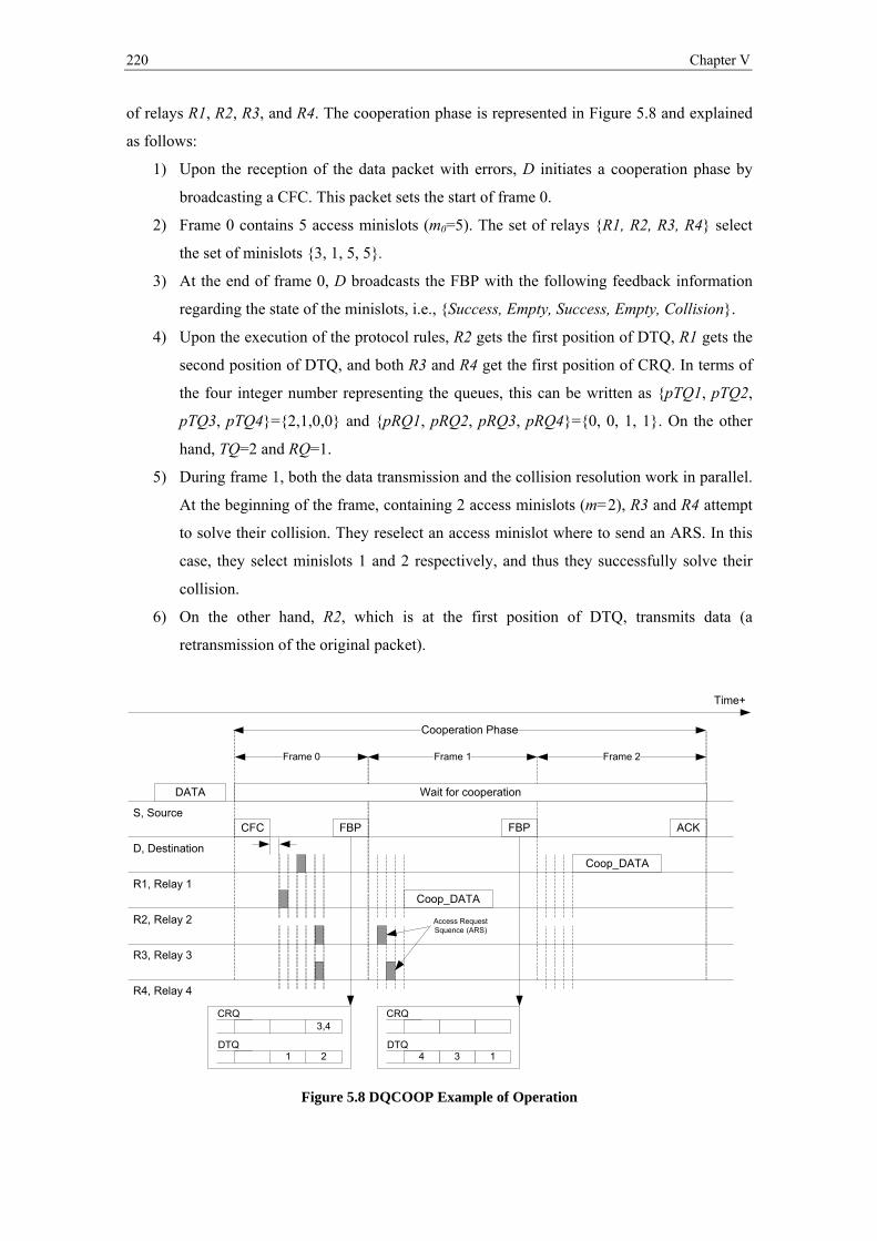
Chapter V
220
of relays R1, R2, R3, and R4. The cooperation phase is represented in Figure 5.8 and explained
as follows:
1) Upon the reception of the data packet with errors, D initiates a cooperation phase by
broadcasting a CFC. This packet sets the start of frame 0.
2) Frame 0 contains 5 access minislots (m0=5). The set of relays {R1, R2, R3, R4} select
the set of minislots {3, 1, 5, 5}.
3) At the end of frame 0, D broadcasts the FBP with the following feedback information
regarding the state of the minislots, i.e., {Success, Empty, Success, Empty, Collision}.
4) Upon the execution of the protocol rules, R2 gets the first position of DTQ, R1 gets the
second position of DTQ, and both R3 and R4 get the first position of CRQ. In terms of
the four integer number representing the queues, this can be written as {pTQ1, pTQ2,
pTQ3, pTQ4}={2,1,0,0} and {pRQ1, pRQ2, pRQ3, pRQ4}={0, 0, 1, 1}. On the other
hand, TQ=2 and RQ=1.
5) During frame 1, both the data transmission and the collision resolution work in parallel.
At the beginning of the frame, containing 2 access minislots (m=2), R3 and R4 attempt
to solve their collision. They reselect an access minislot where to send an ARS. In this
case, they select minislots 1 and 2 respectively, and thus they successfully solve their
collision.
6) On the other hand, R2, which is at the first position of DTQ, transmits data (a
retransmission of the original packet).
Coop_DATA
FBP
Time+
CFC
Coop_DATA
ACK
Cooperation Phase
FBP
R1, Relay 1
S, Source
DATA
D, Destination
R2, Relay 2
R3, Relay 3
R4, Relay 4
21DTQ
3,4CRQ
134DTQ
CRQ
Frame 0 Frame 1 Frame 2
Wait for cooperation
Access Request Squence (ARS)
Figure 5.8 DQCOOP Example of Operation
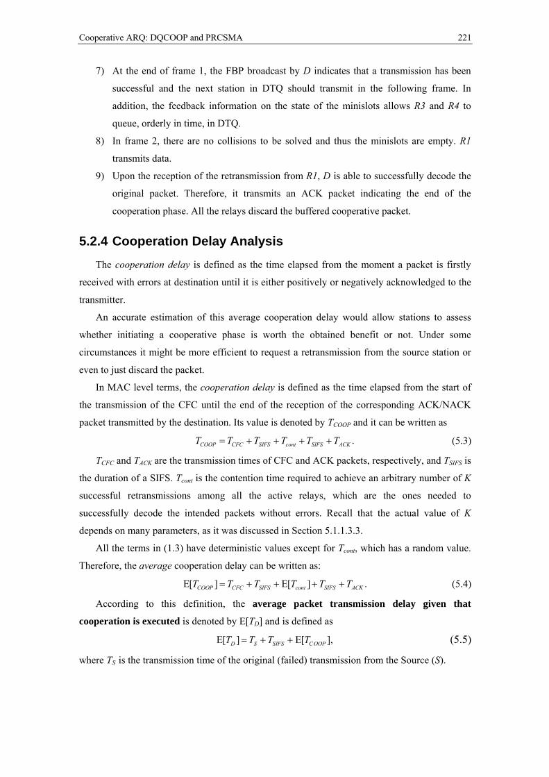
Cooperative ARQ: DQCOOP and PRCSMA 221
7) At the end of frame 1, the FBP broadcast by D indicates that a transmission has been
successful and the next station in DTQ should transmit in the following frame. In
addition, the feedback information on the state of the minislots allows R3 and R4 to
queue, orderly in time, in DTQ.
8) In frame 2, there are no collisions to be solved and thus the minislots are empty. R1
transmits data.
9) Upon the reception of the retransmission from R1, D is able to successfully decode the
original packet. Therefore, it transmits an ACK packet indicating the end of the
cooperation phase. All the relays discard the buffered cooperative packet.
5.2.4 Cooperation Delay Analysis
The cooperation delay is defined as the time elapsed from the moment a packet is firstly
received with errors at destination until it is either positively or negatively acknowledged to the
transmitter.
An accurate estimation of this average cooperation delay would allow stations to assess
whether initiating a cooperative phase is worth the obtained benefit or not. Under some
circumstances it might be more efficient to request a retransmission from the source station or
even to just discard the packet.
In MAC level terms, the cooperation delay is defined as the time elapsed from the start of
the transmission of the CFC until the end of the reception of the corresponding ACK/NACK
packet transmitted by the destination. Its value is denoted by TCOOP and it can be written as
.COOP CFC SIFS cont SIFS ACKT T T T T T (5.3)
TCFC and TACK are the transmission times of CFC and ACK packets, respectively, and TSIFS is
the duration of a SIFS. Tcont is the contention time required to achieve an arbitrary number of K
successful retransmissions among all the active relays, which are the ones needed to
successfully decode the intended packets without errors. Recall that the actual value of K
depends on many parameters, as it was discussed in Section 5.1.1.3.3.
All the terms in (1.3) have deterministic values except for Tcont, which has a random value.
Therefore, the average cooperation delay can be written as:
E[ ] E[ ] .COOP CFC SIFS cont SIFS ACKT T T T T T (5.4)
According to this definition, the average packet transmission delay given that
cooperation is executed is denoted by E[TD] and is defined as
E[ ] E[ ],D S SIFS COOPT T T T (5.5)
where TS is the transmission time of the original (failed) transmission from the Source (S).
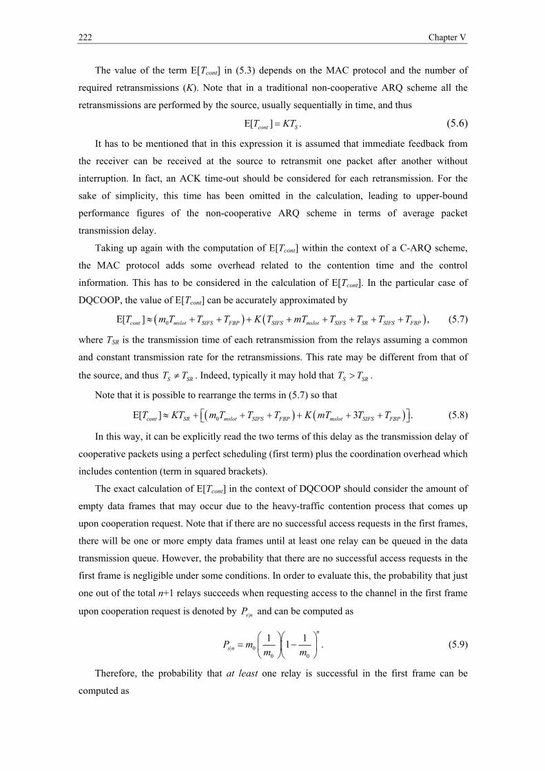
Chapter V
222
The value of the term E[Tcont] in (5.3) depends on the MAC protocol and the number of
required retransmissions (K). Note that in a traditional non-cooperative ARQ scheme all the
retransmissions are performed by the source, usually sequentially in time, and thus
E[ ] .cont ST KT (5.6)
It has to be mentioned that in this expression it is assumed that immediate feedback from
the receiver can be received at the source to retransmit one packet after another without
interruption. In fact, an ACK time-out should be considered for each retransmission. For the
sake of simplicity, this time has been omitted in the calculation, leading to upper-bound
performance figures of the non-cooperative ARQ scheme in terms of average packet
transmission delay.
Taking up again with the computation of E[Tcont] within the context of a C-ARQ scheme,
the MAC protocol adds some overhead related to the contention time and the control
information. This has to be considered in the calculation of E[Tcont]. In the particular case of
DQCOOP, the value of E[Tcont] can be accurately approximated by
0E[ ] ,cont mslot SIFS FBP SIFS mslot SIFS SR SIFS FBPT m T T T K T mT T T T T (5.7)
where TSR is the transmission time of each retransmission from the relays assuming a common
and constant transmission rate for the retransmissions. This rate may be different from that of
the source, and thus S SRT T . Indeed, typically it may hold that S SRT T .
Note that it is possible to rearrange the terms in (5.7) so that
0E[ ] 3 .cont SR mslot SIFS FBP mslot SIFS FBPT KT m T T T K mT T T (5.8)
In this way, it can be explicitly read the two terms of this delay as the transmission delay of
cooperative packets using a perfect scheduling (first term) plus the coordination overhead which
includes contention (term in squared brackets).
The exact calculation of E[Tcont] in the context of DQCOOP should consider the amount of
empty data frames that may occur due to the heavy-traffic contention process that comes up
upon cooperation request. Note that if there are no successful access requests in the first frames,
there will be one or more empty data frames until at least one relay can be queued in the data
transmission queue. However, the probability that there are no successful access requests in the
first frame is negligible under some conditions. In order to evaluate this, the probability that just
one out of the total n+1 relays succeeds when requesting access to the channel in the first frame
upon cooperation request is denoted by |s nP and can be computed as
| 00 0
1 11 .
n
s nP mm m
(5.9)
Therefore, the probability that at least one relay is successful in the first frame can be
computed as
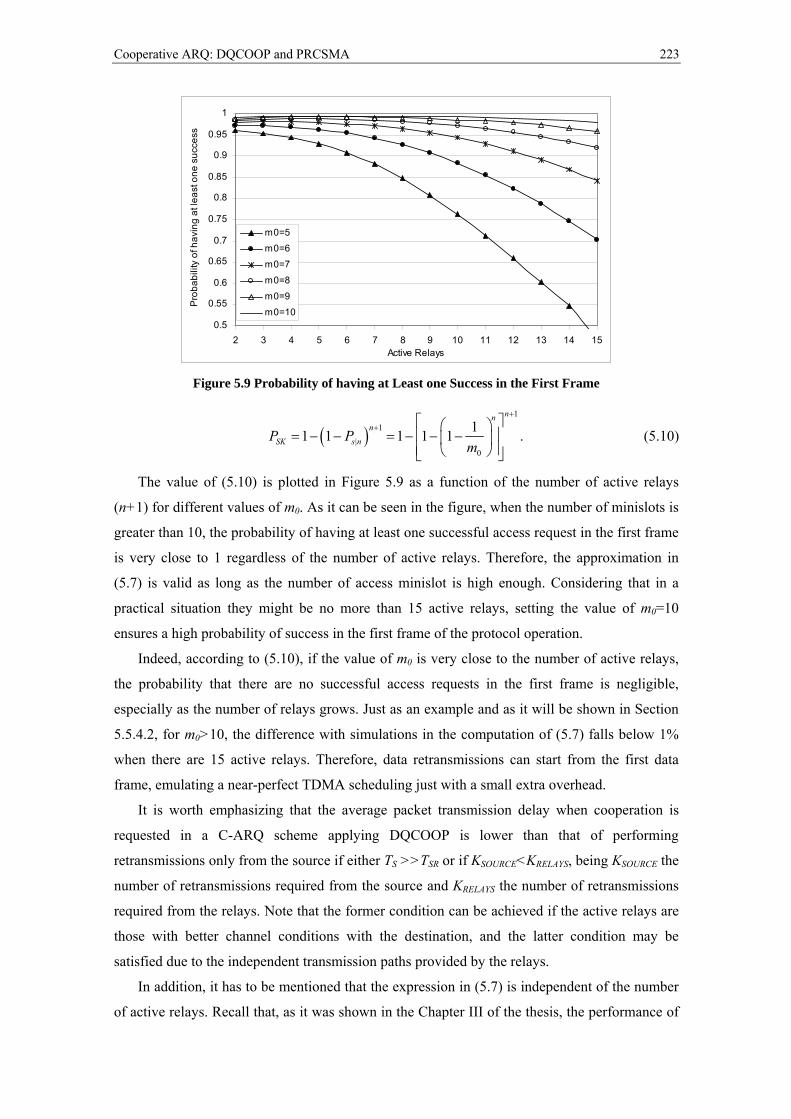
Cooperative ARQ: DQCOOP and PRCSMA 223
0.5
0.55
0.6
0.65
0.7
0.75
0.8
0.85
0.9
0.95
1
2 3 4 5 6 7 8 9 10 11 12 13 14 15Active Relays
Pro
ba
bili
ty o
f ha
vin
g a
t le
ast
on
e s
ucc
ess
m0=5
m0=6
m0=7
m0=8
m0=9
m0=10
Figure 5.9 Probability of having at Least one Success in the First Frame
1
1
|0
11 1 1 1 1 .
nnn
SK s nP Pm
(5.10)
The value of (5.10) is plotted in Figure 5.9 as a function of the number of active relays
(n+1) for different values of m0. As it can be seen in the figure, when the number of minislots is
greater than 10, the probability of having at least one successful access request in the first frame
is very close to 1 regardless of the number of active relays. Therefore, the approximation in
(5.7) is valid as long as the number of access minislot is high enough. Considering that in a
practical situation they might be no more than 15 active relays, setting the value of m0=10
ensures a high probability of success in the first frame of the protocol operation.
Indeed, according to (5.10), if the value of m0 is very close to the number of active relays,
the probability that there are no successful access requests in the first frame is negligible,
especially as the number of relays grows. Just as an example and as it will be shown in Section
5.5.4.2, for m0>10, the difference with simulations in the computation of (5.7) falls below 1%
when there are 15 active relays. Therefore, data retransmissions can start from the first data
frame, emulating a near-perfect TDMA scheduling just with a small extra overhead.
It is worth emphasizing that the average packet transmission delay when cooperation is
requested in a C-ARQ scheme applying DQCOOP is lower than that of performing
retransmissions only from the source if either TS >>TSR or if KSOURCE<KRELAYS, being KSOURCE the
number of retransmissions required from the source and KRELAYS the number of retransmissions
required from the relays. Note that the former condition can be achieved if the active relays are
those with better channel conditions with the destination, and the latter condition may be
satisfied due to the independent transmission paths provided by the relays.
In addition, it has to be mentioned that the expression in (5.7) is independent of the number
of active relays. Recall that, as it was shown in the Chapter III of the thesis, the performance of
Chapter V
224
DQMAN is independent of the number of stations, and DQCOOP keeps this property. This is a
major characteristic of the protocol, especially for its application in C-ARQ schemes, since it
alleviates the requirements of the relay selection algorithm.
The approximation in (5.7) is validated in the next section by comparing its values with the
ones obtained through link-level computer simulation with MACSWIN. In addition, the
performance of DQCOOP under different scenario configurations is also evaluated.
5.2.5 Model Validation and Performance Evaluation
The performance of DQCOOP is evaluated in this section. The average cooperation delay is
calculated both with (5.7) and through computer simulations in MACSWIN where the protocol
rules are actually executed without any approximation. The values of the parameters used both
to compute (5.7) and to configure the simulations are summarized in Table 5.3.
In order to focus on the evaluation of the cooperation phases, a single-hop network wherein
all the data transmissions from a fixed source to a fixed destination are received with errors is
considered. That is, the destination always broadcasts a CFC packet upon the reception of every
original data packet received from the source station. Moreover, the source has always a packet
ready to be transmitted to the destination.
In addition, it is assumed that a constant number of potential relays are activated within
each cooperation phase. Furthermore, and without loss of generality, the destination is
considered to require a constant number of retransmissions from the relay set to decode the
original packet. Recall that the number of retransmissions is denoted by K and that the actual
value of this parameter depends on the channel conditions, the forwarding scheme executed by
the relays, and the combination technique applied at destination to efficiently combine the
different copies received from the relay set.
The accuracy of the computation of the average cooperation delay computed in Section
5.2.4 is assessed in the next section. Then, the performance evaluation is focused on the
evaluation of two configuration parameters of DQCOOP which may have a greater influence on
the performance of the protocol: m and m0. The results are presented in the following
subsections. The comparison of a C-ARQ scheme with DQCOOP and a traditional non-
cooperative ARQ scheme is left for Section 5.4.
Table 5.3 Simulation Parameters (DQCOOP)
Parameter Value Parameter Value Control Rate 6 Mbps MAC header 34 bytes
Data Rate (Source) 24 Mbps PHY preamble 96 μs
Data Rate (Relays) 54 Mbps ACK, CFC, FBP
length 14 bytes
Packet Length 1500 bytes SlotTime 10 μs ARS 10 μs SIFS 10 μs
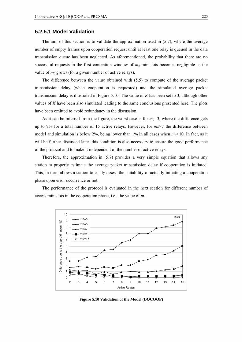
Cooperative ARQ: DQCOOP and PRCSMA 225
5.2.5.1 Model Validation
The aim of this section is to validate the approximation used in (5.7), where the average
number of empty frames upon cooperation request until at least one relay is queued in the data
transmission queue has been neglected. As aforementioned, the probability that there are no
successful requests in the first contention window of m0 minislots becomes negligible as the
value of m0 grows (for a given number of active relays).
The difference between the value obtained with (5.5) to compute of the average packet
transmission delay (when cooperation is requested) and the simulated average packet
transmission delay is illustrated in Figure 5.10. The value of K has been set to 3, although other
values of K have been also simulated leading to the same conclusions presented here. The plots
have been omitted to avoid redundancy in the discussion.
As it can be inferred from the figure, the worst case is for m0=3, where the difference gets
up to 9% for a total number of 15 active relays. However, for m0>7 the difference between
model and simulation is below 2%, being lower than 1% in all cases when m0>10. In fact, as it
will be further discussed later, this condition is also necessary to ensure the good performance
of the protocol and to make it independent of the number of active relays.
Therefore, the approximation in (5.7) provides a very simple equation that allows any
station to properly estimate the average packet transmission delay if cooperation is initiated.
This, in turn, allows a station to easily assess the suitability of actually initiating a cooperation
phase upon error occurrence or not.
The performance of the protocol is evaluated in the next section for different number of
access minislots in the cooperation phase, i.e., the value of m.
0
1
2
3
4
5
6
7
8
9
10
2 3 4 5 6 7 8 9 10 11 12 13 14 15
Active Relays
Diff
ere
nce
du
e to
the
ap
pro
xim
atio
n (
%) m0=3
m0=5
m0=7
m0=10
m0=15
K=3
Figure 5.10 Validation of the Model (DQCOOP)
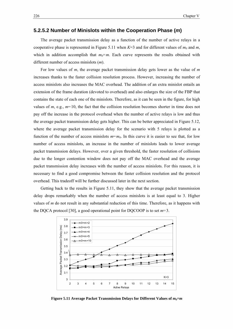
Chapter V
226
5.2.5.2 Number of Minislots within the Cooperation Phase (m)
The average packet transmission delay as a function of the number of active relays in a
cooperative phase is represented in Figure 5.11 when K=3 and for different values of m0 and m,
which in addition accomplish that m0=m. Each curve represents the results obtained with
different number of access minislots (m).
For low values of m, the average packet transmission delay gets lower as the value of m
increases thanks to the faster collision resolution process. However, increasing the number of
access minislots also increases the MAC overhead. The addition of an extra minislot entails an
extension of the frame duration (devoted to overhead) and also enlarges the size of the FBP that
contains the state of each one of the minislots. Therefore, as it can be seen in the figure, for high
values of m, e.g., m=10, the fact that the collision resolution becomes shorter in time does not
pay off the increase in the protocol overhead when the number of active relays is low and thus
the average packet transmission delay gets higher. This can be better appreciated in Figure 5.12,
where the average packet transmission delay for the scenario with 5 relays is plotted as a
function of the number of access minislots m=m0. In this curve it is easier to see that, for low
number of access minislots, an increase in the number of minislots leads to lower average
packet transmission delays. However, over a given threshold, the faster resolution of collisions
due to the longer contention window does not pay off the MAC overhead and the average
packet transmission delay increases with the number of access minislots. For this reason, it is
necessary to find a good compromise between the faster collision resolution and the protocol
overhead. This tradeoff will be further discussed later in the next section.
Getting back to the results in Figure 5.11, they show that the average packet transmission
delay drops remarkably when the number of access minislots is at least equal to 3. Higher
values of m do not result in any substantial reduction of this time. Therefore, as it happens with
the DQCA protocol [30], a good operational point for DQCOOP is to set m=3.
3
3.1
3.2
3.3
3.4
3.5
3.6
3.7
3.8
3.9
2 3 4 5 6 7 8 9 10 11 12 13 14 15
Active Relays
Ave
rag
e P
ack
et T
ran
smis
sio
n D
ela
y (m
s)
m0=m=2
m0=m=3
m0=m=4
m0=m=5
m0=m=10
K=3
Figure 5.11 Average Packet Transmission Delays for Different Values of m0=m
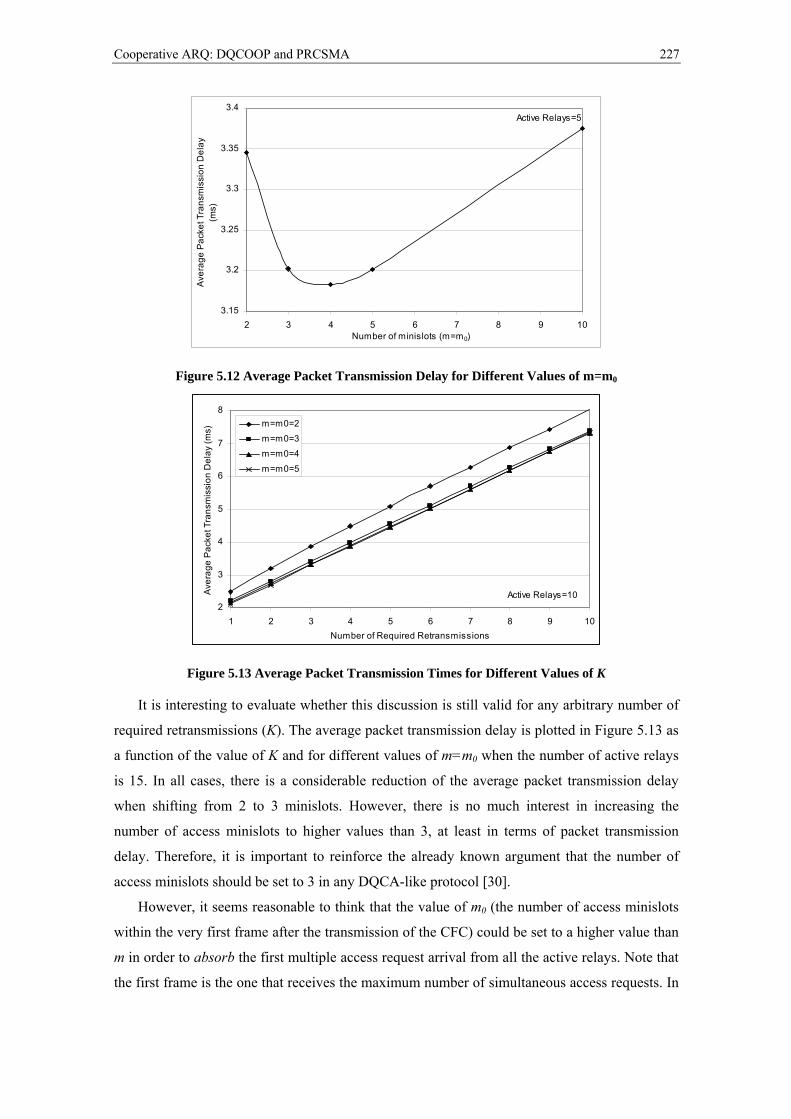
Cooperative ARQ: DQCOOP and PRCSMA 227
Active Relays=5
3.15
3.2
3.25
3.3
3.35
3.4
2 3 4 5 6 7 8 9 10Number of minislots (m=m0)
Ave
rag
e P
ack
et T
ran
smis
sio
n D
ela
y (m
s)
Figure 5.12 Average Packet Transmission Delay for Different Values of m=m0
2
3
4
5
6
7
8
1 2 3 4 5 6 7 8 9 10
Number of Required Retransmissions
Ave
rag
e P
ack
et T
ran
smis
sio
n D
ela
y (m
s)
m=m0=2
m=m0=3
m=m0=4
m=m0=5
Active Relays=10
Figure 5.13 Average Packet Transmission Times for Different Values of K
It is interesting to evaluate whether this discussion is still valid for any arbitrary number of
required retransmissions (K). The average packet transmission delay is plotted in Figure 5.13 as
a function of the value of K and for different values of m=m0 when the number of active relays
is 15. In all cases, there is a considerable reduction of the average packet transmission delay
when shifting from 2 to 3 minislots. However, there is no much interest in increasing the
number of access minislots to higher values than 3, at least in terms of packet transmission
delay. Therefore, it is important to reinforce the already known argument that the number of
access minislots should be set to 3 in any DQCA-like protocol [30].
However, it seems reasonable to think that the value of m0 (the number of access minislots
within the very first frame after the transmission of the CFC) could be set to a higher value than
m in order to absorb the first multiple access request arrival from all the active relays. Note that
the first frame is the one that receives the maximum number of simultaneous access requests. In
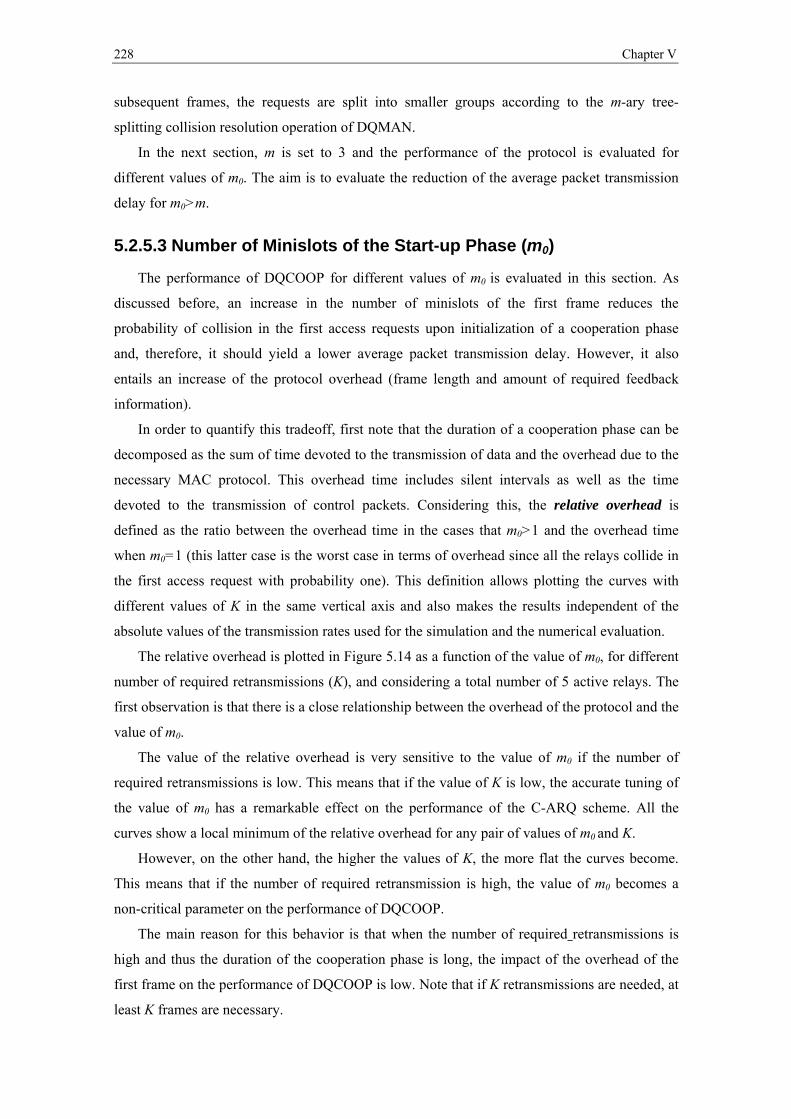
Chapter V
228
subsequent frames, the requests are split into smaller groups according to the m-ary tree-
splitting collision resolution operation of DQMAN.
In the next section, m is set to 3 and the performance of the protocol is evaluated for
different values of m0. The aim is to evaluate the reduction of the average packet transmission
delay for m0>m.
5.2.5.3 Number of Minislots of the Start-up Phase (m0)
The performance of DQCOOP for different values of m0 is evaluated in this section. As
discussed before, an increase in the number of minislots of the first frame reduces the
probability of collision in the first access requests upon initialization of a cooperation phase
and, therefore, it should yield a lower average packet transmission delay. However, it also
entails an increase of the protocol overhead (frame length and amount of required feedback
information).
In order to quantify this tradeoff, first note that the duration of a cooperation phase can be
decomposed as the sum of time devoted to the transmission of data and the overhead due to the
necessary MAC protocol. This overhead time includes silent intervals as well as the time
devoted to the transmission of control packets. Considering this, the relative overhead is
defined as the ratio between the overhead time in the cases that m0>1 and the overhead time
when m0=1 (this latter case is the worst case in terms of overhead since all the relays collide in
the first access request with probability one). This definition allows plotting the curves with
different values of K in the same vertical axis and also makes the results independent of the
absolute values of the transmission rates used for the simulation and the numerical evaluation.
The relative overhead is plotted in Figure 5.14 as a function of the value of m0, for different
number of required retransmissions (K), and considering a total number of 5 active relays. The
first observation is that there is a close relationship between the overhead of the protocol and the
value of m0.
The value of the relative overhead is very sensitive to the value of m0 if the number of
required retransmissions is low. This means that if the value of K is low, the accurate tuning of
the value of m0 has a remarkable effect on the performance of the C-ARQ scheme. All the
curves show a local minimum of the relative overhead for any pair of values of m0 and K.
However, on the other hand, the higher the values of K, the more flat the curves become.
This means that if the number of required retransmission is high, the value of m0 becomes a
non-critical parameter on the performance of DQCOOP.
The main reason for this behavior is that when the number of required retransmissions is
high and thus the duration of the cooperation phase is long, the impact of the overhead of the
first frame on the performance of DQCOOP is low. Note that if K retransmissions are needed, at
least K frames are necessary.
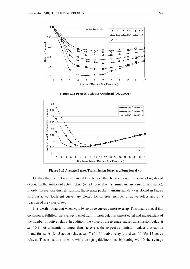
Cooperative ARQ: DQCOOP and PRCSMA 229
0.75
0.8
0.85
0.9
0.95
1
1 2 3 4 5 6 7 8 9 10 11 12
Number of Minislots First Frame (m0)
Re
lativ
e O
verh
ea
d
K=1 K=2 K=3
K=4 K=5 K=6
K=7
Active Relays=5
Figure 5.14 Protocol Relative Overhead (DQCOOP)
3.1
3.15
3.2
3.25
3.3
3.35
3.4
3.45
3.5
2 3 4 5 6 7 8 9 10 11 12 13 14 15 16 17 18 19 20
Number of Access Minislots First Frame (m0)
Ave
rag
e P
ack
et T
ran
smis
sio
n D
ela
y (m
s)
Active Relays=5
Active Relays=10
Active Relays=15
K=3
Figure 5.15 Average Packet Transmission Delay as a Function of m0
On the other hand, it seems reasonable to believe that the selection of the value of m0 should
depend on the number of active relays (which request access simultaneously in the first frame).
In order to evaluate this relationship, the average packet transmission delay is plotted in Figure
5.15 for K =3. Different curves are plotted for different number of active relays and as a
function of the value of m0.
It is worth noting that when 0 10m the three curves almost overlap. This means that, if this
condition is fulfilled, the average packet transmission delay is almost equal and independent of
the number of active relays. In addition, the value of the average packet transmission delay at
m0=10 is not substantially bigger than the one at the respective minimum values that can be
found for m0=6 (for 5 active relays), m0=7 (for 10 active relays), and m0=10 (for 15 active
relays). This constitutes a worthwhile design guideline since by setting m0=10 the average
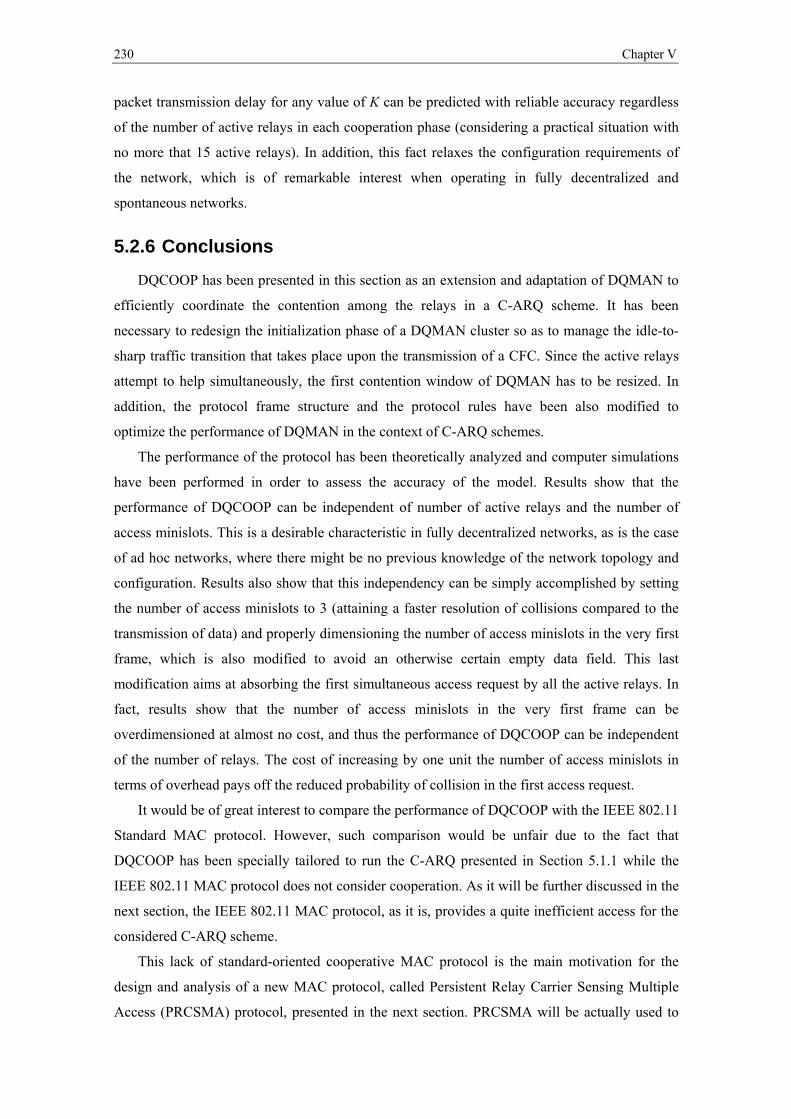
Chapter V
230
packet transmission delay for any value of K can be predicted with reliable accuracy regardless
of the number of active relays in each cooperation phase (considering a practical situation with
no more that 15 active relays). In addition, this fact relaxes the configuration requirements of
the network, which is of remarkable interest when operating in fully decentralized and
spontaneous networks.
5.2.6 Conclusions
DQCOOP has been presented in this section as an extension and adaptation of DQMAN to
efficiently coordinate the contention among the relays in a C-ARQ scheme. It has been
necessary to redesign the initialization phase of a DQMAN cluster so as to manage the idle-to-
sharp traffic transition that takes place upon the transmission of a CFC. Since the active relays
attempt to help simultaneously, the first contention window of DQMAN has to be resized. In
addition, the protocol frame structure and the protocol rules have been also modified to
optimize the performance of DQMAN in the context of C-ARQ schemes.
The performance of the protocol has been theoretically analyzed and computer simulations
have been performed in order to assess the accuracy of the model. Results show that the
performance of DQCOOP can be independent of number of active relays and the number of
access minislots. This is a desirable characteristic in fully decentralized networks, as is the case
of ad hoc networks, where there might be no previous knowledge of the network topology and
configuration. Results also show that this independency can be simply accomplished by setting
the number of access minislots to 3 (attaining a faster resolution of collisions compared to the
transmission of data) and properly dimensioning the number of access minislots in the very first
frame, which is also modified to avoid an otherwise certain empty data field. This last
modification aims at absorbing the first simultaneous access request by all the active relays. In
fact, results show that the number of access minislots in the very first frame can be
overdimensioned at almost no cost, and thus the performance of DQCOOP can be independent
of the number of relays. The cost of increasing by one unit the number of access minislots in
terms of overhead pays off the reduced probability of collision in the first access request.
It would be of great interest to compare the performance of DQCOOP with the IEEE 802.11
Standard MAC protocol. However, such comparison would be unfair due to the fact that
DQCOOP has been specially tailored to run the C-ARQ presented in Section 5.1.1 while the
IEEE 802.11 MAC protocol does not consider cooperation. As it will be further discussed in the
next section, the IEEE 802.11 MAC protocol, as it is, provides a quite inefficient access for the
considered C-ARQ scheme.
This lack of standard-oriented cooperative MAC protocol is the main motivation for the
design and analysis of a new MAC protocol, called Persistent Relay Carrier Sensing Multiple
Access (PRCSMA) protocol, presented in the next section. PRCSMA will be actually used to
Cooperative ARQ: DQCOOP and PRCSMA 231
have a feasible benchmark reference. It is based on the fundamental operation of the IEEE
802.11 Standard protocol and it can be considered as the extension and adaptation of the
protocol to meet the requirements of the C-ARQ scheme.
The comparison between DQCOOP and PRCSMA is left for Section 5.4. In that section, the
performance of the two protocols will be also compared to that of a traditional non-cooperative
ARQ scheme and that of an ideal C-ARQ with perfect TDMA scheduling among the relays.
5.3 PRCSMA: Persistent Relay CSMA Protocol
5.3.1 Introduction and Problem Statement
The IEEE 802.11 MAC protocol has not been specifically designed to be executed in C-
ARQ schemes. It provides fair long-term access and runs in stable conditions over WLANs
(with limited number of active users and under not very heavy traffic conditions). However, if it
was used in the C-ARQ scheme like the one considered in this chapter, it would provide a
highly inefficient access operation. For example, assume that there is no virtual carrier sensing
mechanism. In this situation cooperation would be possible. Otherwise, stations are oblivious to
transmissions not directed to them and thus cooperation cannot be executed. Therefore, upon
the transmission of a CFC, all the active relays would attempt to transmit after a DIFS period.
This would result in an unavoidable collision. All the active relays would then double up their
contention window, which would lead to an unnecessary increase of the transmission delay.
Considering the drawbacks of the standard MAC protocol for its use in the C-ARQ scheme,
the Persistent Relay Carrier Sensing Multiple Access (PRCSMA) is presented in this section as
an extension and adaptation of the IEEE 802.11 MAC protocol to meet the requirements of the
C-ARQ scheme described in Section 5.1.1.
The main objective now is to define a novel MAC protocol that can be implemented in off-
the-shelf 802.11 wireless cards by slightly modifying the wireless controller. The main design
goal of PRCSMA is to enable stations equipped with an IEEE 802.11 interface to ask their
neighbors to cooperate upon the erroneous reception of a data packet. This cooperation will
result in a C-ARQ scheme. Therefore, the key objective is to slightly modify the legacy IEEE
802.11 MAC rules to enable cooperation among the stations in a way that they could be easily
backwards compatible.
The rest of this section is organized as follows. PRCSMA is described in Section 5.3.2.
Rather than presenting a comprehensive description, for the sake of simplicity and brevity, it is
assumed that the reader is already familiar with the IEEE 802.11 MAC protocol which was
summarized in Chapter IV, and the focus is put just on the modifications necessary to meet the
requirements of the C-ARQ scheme. In Section 5.3.3, an operational example of PRCSMA is
presented to help in the understanding of the overall protocol operation. The average
Chapter V
232
cooperation delay of PRCSMA is analyzed in Section 5.3.4. The computation is validated in
Section 5.3.5 by comparing the analytical results with computer simulations. An exhaustive
performance evaluation of the protocol is also presented in that section. Section 5.3.6 concludes
the section and gives some final remarks.
5.3.2 Protocol Description
Whenever a data packet is received with errors at a destination station, a cooperation phase
is initiated by this station by broadcasting a CFC packet. Upon the reception of the CFC, some
stations become active relays. These relays will try to get access to the channel in order to
retransmit the data packet (cooperative packets) until the destination can decode the packet, or it
discards it. The relay selection criterion can be whatever desired and the definition of a specific
one is out of the scope of the description of PRCSMA. Active relays just execute the MAC rules
specified in the IEEE 802.11 Standard [9] to get access to the channel, but considering the two
following modifications:
1) Active relays perform a backoff period before attempting to transmit for the first time
upon the reception of the CFC. This is necessary since the sub-network formed by the
relays works in saturation conditions, i.e., all the active relays always have a data packet
ready to be transmitted during a cooperation phase. Then, it is necessary to execute a
backoff at the beginning of the cooperation phase in order to avoid a certain collision.
The duration of this initial backoff period is selected within the minimum contention
window upon the reception of a CFC packet.
2) There is no expected ACK associated to each transmitted cooperation packet.
A cooperation phase can be finished whenever one out of these two events occurs:
1) The destination station is able to decode the original data packet by properly combining
the different cooperative packets received from the relay set (or because an error-free
copy is received from a relay).
2) A certain maximum cooperation time-out has elapsed and the original packet is
discarded.
In the former case, an ACK packet is transmitted by the destination. In the latter case, a
negative ACK (NACK) is transmitted by the destination. In any case, the cooperation phase is
finished and all the relays pop out the cooperative packet from their queue upon the end of a
cooperation phase.
According to all this operation, three implementation issues should be considered:
1) The CFC can be a regular RTS packet, using the empty field for address 4, as done in
[23], to distinguish the packet from a normal RTS.
2) As long as there is at least one active relay, the persistent behavior of PRCSMA
eliminates the probability that the destination station does not receive the required
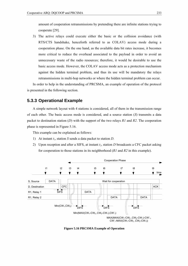
Cooperative ARQ: DQCOOP and PRCSMA 233
amount of cooperation retransmissions by pretending there are infinite stations trying to
cooperate [29].
3) The active relays could execute either the basic or the collision avoidance (with
RTS/CTS handshake, henceforth referred to as COLAV) access mode during a
cooperation phase. On the one hand, as the available data bit rates increase, it becomes
more critical to reduce the overhead associated to the payload in order to avoid an
unnecessary waste of the radio resources; therefore, it would be desirable to use the
basic access mode. However, the COLAV access mode acts as a protection mechanism
against the hidden terminal problem, and thus its use will be mandatory the relays
retransmissions in multi-hop networks or where the hidden terminal problem can occur.
In order to help in the understanding of PRCSMA, an example of operation of the protocol
is presented in the following section.
5.3.3 Operational Example
A simple network layout with 4 stations is considered, all of them in the transmission range
of each other. The basic access mode is considered, and a source station (S) transmits a data
packet to destination station (D) with the support of the two relays R1 and R2. The cooperation
phase is represented in Figure 5.16.
This example can be explained as follows:
1) At instant t1, station S sends a data packet to station D.
2) Upon reception and after a SIFS, at instant t2, station D broadcasts a CFC packet asking
for cooperation to those stations in its neighborhood (R1 and R2 in this example).
DATA
CFC
DATA
D, Destination
R1, Relay 1
R1, Relay 2
Min(CW1,CW2)
DATA
ACK
S, Source Wait for cooperation
DIFS
Min(MAX(CW1-CW2 ,CW2-CW1),CW’1)
SIFS
DIFS
MAX(MAX(CW1-CW2 ,CW2-CW1)-CW’1, CW’1-MAX(CW1-CW2 ,CW2-CW1))
DATA
DIFS
time
t1 t2 t3 t4 t5 t6 t7 t8 t9
Cooperation Phase
Figure 5.16 PRCSMA Example of Operation
Chapter V
234
3) Stations R1 and R2 receive the CFC packet and set up their backoff counters CW1 and
CW2, respectively, at instant t3. S waits for the cooperation phase to finish.
4) At instant t4, the backoff counter of R1 expires (CW1) and R1 attempts to transmit a
copy of the requested packet.
5) At instant t5, R2 resumes the backoff counter while R1 resets a new value for its backoff
counter (CW’1)
6) At instant t6, the backoff counter of R2 expires and R2 attempts to transmit the copy of
the requested packet.
7) At instant t7, R1 resumes the backoff counter and R2 resets a new backoff counter.
8) At instant t8, the backoff counter of R2 expires and R2 attempts to transmit a copy of the
requested packet.
9) At instant t9, station D is able to properly decode the original data packet and sends
back an ACK packet, indicating the end of the cooperation phase. All the stations then
know that the cooperation phase has ended.
5.3.4 Cooperation Delay Analysis
5.3.4.1 Introduction
The average cooperation delay, as defined in Section 5.2.4, is analytically evaluated in this
section. Recall that it was defined as the time elapsed from the moment a packet is received
with errors, until it is acknowledged to the transmitter right after it has been properly decoded
by combining the different retransmissions received from the relays at destination.
Therefore, in MAC protocol terms, the average cooperation delay is defined as the
average time elapsed from the start of the transmission of a CFC until the end of the
transmission of the ACK packet by the destination station. This average delay is denoted by
E[TCOOP] and it can be computed as
E[ ] E[ ] .COOP CFC SIFS cont SIFS ACKT T T T T T (5.11)
Recall that TCFC and TACK are the transmission times of CFC and ACK packets, respectively,
and TSIFS is the duration of a SIFS. E[Tcont] is the average contention time required to achieve an
arbitrary number of K successful retransmissions among the relays. According to this definition,
the average packet transmission delay given that cooperation is executed is denoted by
E[TD] and defined as
E[ ] E[ ],D S SIFS COOPT T T T (5.12)
where TS is the transmission time of the original failed transmission from the Source (S). The
value of the term E[Tcont] in (5.11) depends on the MAC protocol and the number of required
retransmissions, K. Recall that in a traditional non-cooperative ARQ scheme all the
retransmissions are performed by the source and, typically sequentially in time, and thus
Cooperative ARQ: DQCOOP and PRCSMA 235
E[ ] .cont ST KT (5.13)
Also recall that in this expression it is assumed that immediate feedback from the receiver
can be received at the source to retransmit one packet after another without interruption. In fact,
an ACK time-out should be considered for each retransmission. For the sake of simplicity, this
time has been omitted in the calculation, leading to upper-bound performance figures of the
non-cooperative ARQ scheme in terms of average packet transmission delay.
Taking up again with the computation of E[Tcont] within the context of a C-ARQ scheme,
the MAC protocol adds some overhead related to the contention time and the control
information. This overhead has to be considered in the calculation of E[Tcont]. The expectation
of the duration of the contention phase is computed in this section in the context of PRCSMA.
To do so, it has to be considered that, upon the reception of a CFC packet, some of the
stations which received the original transmission from the source without errors become active
relays and they attempt to transmit a copy of the original packet as many times as necessary
until the cooperation phase is over. It is considered that the CFC packet must be received over a
certain SNR threshold so that a potential relay decides to become active in a given cooperation
phase. Henceforth, it is assumed that this threshold is such that all the active relays are within
the transmission range of each other, avoiding thus the presence of hidden terminals.
The sub-network formed by the active relays works in saturation conditions for the whole
cooperative phase until the destination station is able to decode the packet. Although there are in
the literature several models that allow computing the saturation performance of an IEEE
802.11 ad hoc network [32]-[36], none of them is suitable to model PRCSMA. Indeed, all these
models compute the saturation throughput of a network in steady state conditions. However, the
fact that when using PRCSMA all the active stations reset their contention window upon the
end of any cooperation phase requires the analysis of the start-up transient period of the
network. This analysis, which has not been yet tackled in the literature, is presented in the next
section within the context of PRCSMA.
5.3.4.2 PRCSMA Model
Consider the sub-network formed by a relay set of n stations, all of them in the transmission
range of each other. In order to focus on the analysis of this sub-network, it is considered that
cooperation phases are executed one after another, i.e., all the initial transmissions from the
source station (none of the relays) are always received with errors at the intended destination.
This approach allows isolating the cooperative phases, which is the focus of the analysis herein
presented. In addition, it is assumed that all the relays transmit at a common constant
transmission rate for both data and control.
During each cooperation phase all the relays persistently attempt to transmit a packet and,
therefore, every station is either transmitting or in backoff. The main assumption of the
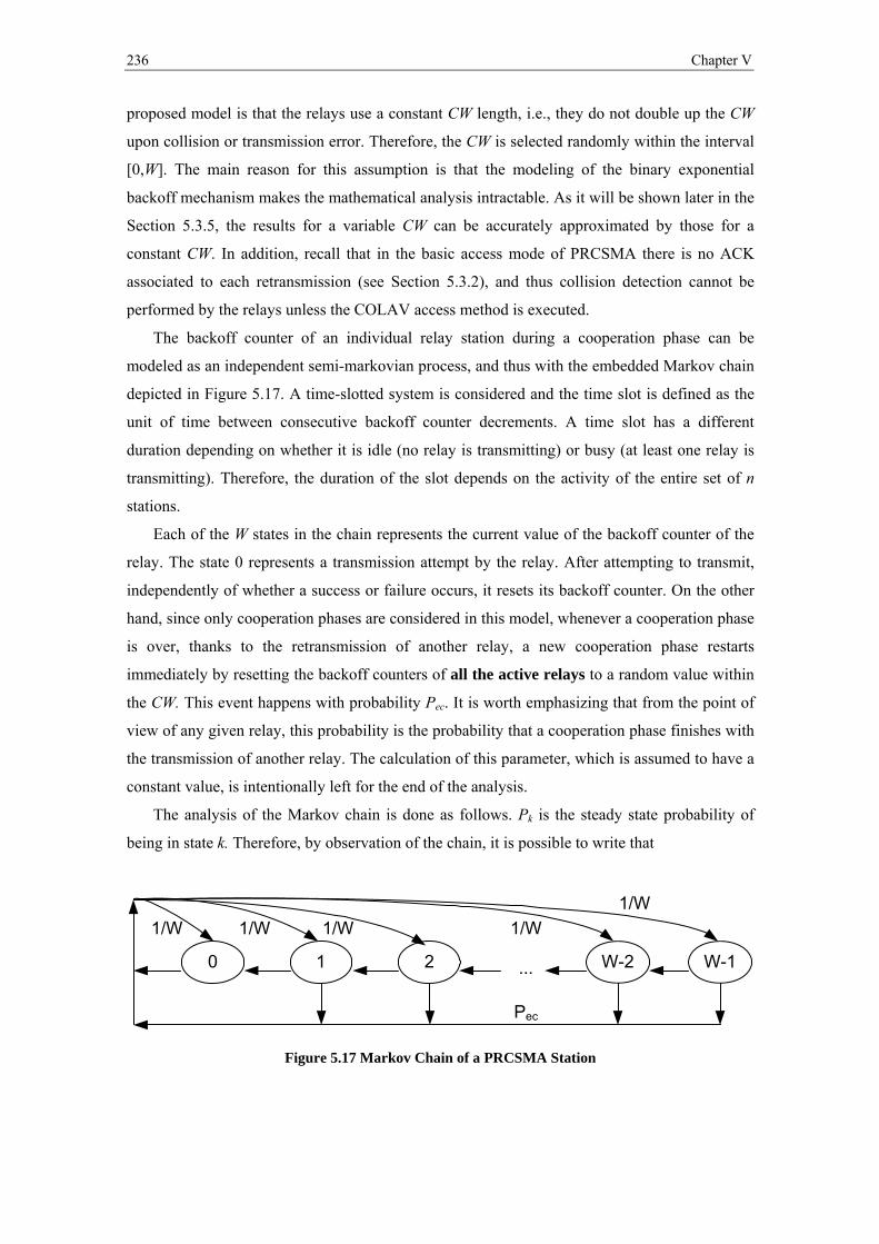
Chapter V
236
proposed model is that the relays use a constant CW length, i.e., they do not double up the CW
upon collision or transmission error. Therefore, the CW is selected randomly within the interval
[0,W]. The main reason for this assumption is that the modeling of the binary exponential
backoff mechanism makes the mathematical analysis intractable. As it will be shown later in the
Section 5.3.5, the results for a variable CW can be accurately approximated by those for a
constant CW. In addition, recall that in the basic access mode of PRCSMA there is no ACK
associated to each retransmission (see Section 5.3.2), and thus collision detection cannot be
performed by the relays unless the COLAV access method is executed.
The backoff counter of an individual relay station during a cooperation phase can be
modeled as an independent semi-markovian process, and thus with the embedded Markov chain
depicted in Figure 5.17. A time-slotted system is considered and the time slot is defined as the
unit of time between consecutive backoff counter decrements. A time slot has a different
duration depending on whether it is idle (no relay is transmitting) or busy (at least one relay is
transmitting). Therefore, the duration of the slot depends on the activity of the entire set of n
stations.
Each of the W states in the chain represents the current value of the backoff counter of the
relay. The state 0 represents a transmission attempt by the relay. After attempting to transmit,
independently of whether a success or failure occurs, it resets its backoff counter. On the other
hand, since only cooperation phases are considered in this model, whenever a cooperation phase
is over, thanks to the retransmission of another relay, a new cooperation phase restarts
immediately by resetting the backoff counters of all the active relays to a random value within
the CW. This event happens with probability Pec. It is worth emphasizing that from the point of
view of any given relay, this probability is the probability that a cooperation phase finishes with
the transmission of another relay. The calculation of this parameter, which is assumed to have a
constant value, is intentionally left for the end of the analysis.
The analysis of the Markov chain is done as follows. Pk is the steady state probability of
being in state k. Therefore, by observation of the chain, it is possible to write that
0 1 2 W-2 W-1
1/W 1/W
1/W
1/W1/W
Pec
...
Figure 5.17 Markov Chain of a PRCSMA Station
Cooperative ARQ: DQCOOP and PRCSMA 237
1
1 01
1
2 0 11
1 1 12
3 0 0 01 1 1
4
1,
11 ,
1 1 11 1 ,
...
W
W k eck
W
W k ec W eck
W W W
W k ec k ec ec k ec eck k k
W
P P P PW
P P P P P PW
P P P P P P P P P P P PW W W
P
(5.14)
Note that the probability that a station attempts to transmit in a given slot is P0 (when the
backoff counter expires). Therefore, it is possible to iteratively obtain the steady state
probability of any state k of the chain as
( 1) 1
00 1
11 .
W k Wj
k i ec ecj i
P P PP PW
(5.15)
According to the Total Probability Theorem, the sum of all the probabilities of the states
must sum to one:
1
01
1.W
kk
P P
(5.16)
Therefore, it is possible to write
( 1)
0 00
( 1)
0 00
11 1
11 1 .
W kj
k ec ecj
W kj
ec ecj
P P P P PW
P P P PW
(5.17)
Using (5.17) in (5.16), it holds that
( 1)1
0 00 0
11 1 1.
W kWj
ec eck j
P P P PW
(5.18)
The interest is on computing the value of P0, i.e., the probability of a transmission attempt,
which can be isolated from
( 1) ( 1)1 1
0 00 0 0 0
1 11 1 1.
W k W kW Wj j
ec ec ec eck j k j
P P P P P PW W
(5.19)
After some algebra, the value of P0 can be expressed as
( 1)1
0 00 ( 1)1
0 0
11
.(1 )
1
W kWj
ec eck j
W kWjec
eck j
W P P
PP
P
(5.20)
In the case that Pec=0, i.e., there is only one active relay, P0 can be written as
Chapter V
238
0 ( 1) 112
00 0
22
11 1
2
2.
211
2
W k WWj
kk j
W W WP
W WW k W
W W
W WW WW
(5.21)
In order to compute this expression, it has been used the fact that
1
( 1).
2
N
n
N Nn
(5.22)
On the other hand, for any Pec>0, i.e., there is more than one active relay and this
probability is not zero, the value of P0 expressed in (5.20) can be simplified as follows. First,
note that for any 0<a<1, it is possible to write that
1
0
1.
1
NNn
n
aa
a
(5.23)
Therefore, the sum terms in (5.20) can be simplified as
( 1)1 1
0 0 0
1 1
0 0
1 (1 )1
1 11 (1 ) (1 ) .
W kW kW Wj ec
eck j k ec
W WW k W k
ec eck kec ec
PP
P
P W PP P
(5.24)
It is possible to make the change of variable j W k and thus
1
0 1
1 1
2
1 1(1 ) (1 )
1 1 1 111 .
W WW k j
ec eck jec ec
W W
ec ec ec ec
ec ec ec
W P W PP P
P WP P PW
P P P
(5.25)
Finally, the value of P0 can be computed as
1
2
0 1
2
1
1
1 1
1
(1 ) 1 1
1 11.
(1 ) 1 1 1
W
ec ec ecec
ecW
ec ec ec ec
ec
W
ec ec ec
Wec ec ec
WP P PW P
PP
P WP P P
P
P P P
P W P P
(5.26)
It is worth noting that this probability depends on the size of the contention window (W)
and also on the probability that a cooperation phase finishes thanks to the successful
transmission from another relay in a given slot (Pec). This last term is still unknown and its
calculation is intentionally left for later in the analysis.
The value of P0 allows for the calculation of the probabilities that a given slot is idle,
Cooperative ARQ: DQCOOP and PRCSMA 239
successful, or collided, in the following manner. Since the operation of each station is
independent of the others, it is possible to compute the probability that a time slot is idle,
successful, or it contains a collision in the following manner. First, p is defined as the
probability of collision seen by any of the n relays in the network when attempting to transmit
in a given slot. As in [32]-[36], it is assumed to have a constant value along time and it is equal
to
101 (1 ) .np P (5.27)
On the other hand, the probability that at least one relay attempts to transmit in a given slot
is given by Ptr and can be expressed as
01 (1 ) ,ntrP P (5.28)
and the probability of having a single transmission in a slot given that a station transmits is
given by ps as
1
0 0(1 ).
n
str
nP Pp
P
(5.29)
Finally, the probabilities that a slot is idle (Pi), that a packet is successfully (no collision)
transmitted in a slot (Ps), and that a collision occurs in a given slot (Pc) can be written as
1 ,
,
1 .
i tr
s tr s
c tr s
P P
P P p
P P p
(5.30)
It is worth mentioning at this point in the analysis that the channel errors can be easily
integrated into the model. Assuming a constant packet error probability denoted by pe, as
previously done in [37]-[42], a non-collided transmission (successful) is received with error
with probability pe, and is successful with probability 1-pe.
The expressions obtained in this section are used in the next section to develop analysis of
the average contention delay, necessary to compute the average cooperation delay expressed in
(5.3).
5.3.4.3 Contention Delay Analysis
Due to the fact that the contention algorithm of PRCSMA is fully distributed, the contention
time of any packet is independent of the contention time of any other packet (from the network
perspective). Therefore, the value of E[Tcont] can be calculated as
E[ ] E[ ] ,cont SR cT K T T (5.31)
where TSR is the duration of a successful transmission from the relays to the destination.
E[Tc] is the average contention time required to transmit a single packet among all the relays,
and K is the number of required retransmissions to recover the failed packet.
Chapter V
240
Recall that the value of K is independent of the MAC layer. It depends on the cooperation
scheme applied at the PHY layer (see Section 5.1.1.3.2), on the type of ARQ scheme applied
(type I or type II, with incremental redundancy), and on the channel conditions between the
source and destination, the source and the relays, and the relays and the destination. On the
other hand, TSR has a constant value that depends on the access method of PRCSMA used by the
relays. It can be computed as
, if basic access
, if COLAV access.DIFS DATA SIFS
SRDIFS RTS SIFS CTS SIFS DATA SIFS
T T TT
T T T T T T T
(5.32)
TDATA is the transmission time of data packet from the relays to the destination. TSIFS and
TDIFS are the duration of a SIFS and DIFS, respectively. TRTS is the transmission time of a RTS
packet and TCTS is the transmission time of a CTS packet.
The focus now is on the computation of the value of E[Tc]. The contention between
successive successful transmissions is composed of a number of idle and collided slots of
different durations. A successful transmission (without collision) is carried out in a given slot
with a probability Ps. Otherwise, with probability (1–Ps) there is no successful transmission.
With this notation, the average number of slots required to achieve a successful transmission
(including the successful one) is denoted by E[X] and it can be calculated as
1
0 0
1E[ ] 1 1 1 .
k k
s s s sk ks s
X k P P P PP P
(5.33)
Then, the total contention time is equal to
| _E[ ] E[ ] 1 ·E[ ],c slot no successT X T (5.34)
where (E[X]–1) is the average number of non-successful slots before having a successful
transmission and | _E[ ]slot no successT is the average duration of a slot given that the slot is not
successful. A slot is not successful if it either idle or collided. Applying Bayes’ theorem, the
average duration of any unsuccessful slot can be expressed as
| _E[ ]1 1
i cslot no success C
s s
P PT T
P P
(5.35)
As previously discussed, a given slot is idle with probability Pi, and its duration is equal to
the basic slot time, denoted by . On the other hand, a given slot suffers a collision among
different stations with probability Pc, and the duration of a collision TC depends on the access
method and it can be written as
_
, if basic access.
, if COLAV accessDIFS DATA SIFS
CDIFS RTS SIFS CTS TIMEOUT
T T TT
T T T T
(5.36)
Cooperative ARQ: DQCOOP and PRCSMA 241
The term TCTS_TIME-OUT is the duration of the CTS time-out period after which a collision is
considered to have occurred if no CTS packet is received by the station transmitting the
corresponding RTS [9].
Therefore, the average total contention time can be rewritten as
1
E[ ] 1 .1 1
i ccont C
s s s
P PT K T
P P P
(5.37)
It is worth recalling that probabilities Ps, Pc, and Pi calculated with (5.30) depend on the
number of active relays n and the size of the backoff window W.
Finally, the last parameter that remains to be computed is Pec. With the observation that a
cooperation phase finishes after K successful transmissions and a successful transmission
occurs, in average, every E[X] slots, it is straightforward to compute Pec as
1
.·E[ ]
sec
PP
K X K (5.38)
At this point, it is possible to compute the average packet transmission delay when
cooperation is requested and PRCSMA is used at the MAC layer. The validation of the model
and the performance evaluation of PRCSMA are presented in the next section.
5.3.5 Model Validation and Performance Evaluation
Computer simulations with MACSWIN have been carried out in order to evaluate the
performance of the protocol. The obtained values also aim to validate the accuracy of the
analytical calculations presented in the previous section and, in turn, of the assumptions
adopted. It has to be mentioned that computer simulations do not use any of the analytical
expressions presented in the previous section but they reproduce the behavior of the protocol
operation. The scenario is described in the next section and the results are presented and
discussed in Section 5.3.5.2.
5.3.5.1 Scenario
The same scenario used for the evaluation of DQCOOP in Section 5.2 has been considered
to evaluate the performance of PRCSMA. It is summarized as follows. In order to focus on the
evaluation of the cooperation phases, a network where all the data transmissions from the
source are received with errors at destination is considered. Therefore, a CFC packet is always
broadcast upon the reception of every original data packet (not if received from the relays). In
addition, it is assumed that a constant number of active relays are activated within each
cooperation phase. The relay criteria are such that the relay set forms a single-hop sub-network
(no-hidden terminals). It is also assumed that any destination station requires a constant number
of retransmissions K to successfully decode the original packet. Recall that the actual value of
Chapter V
242
this parameter depends on the channel conditions, the forwarding scheme executed by the
relays, and the combination technique applied at destination to efficiently combine the different
copies received from the relay set.
The values of the parameters for the evaluation have been set based on the PHY
specifications defined in the IEEE 802.11g standard for WLANs [43], and they are summarized
in Table 5.4.
Table 5.4 System Parameters (PRCSMA)
Parameter Value Parameter Value Control Rate 6 Mbps MAC header 34 bytes
Data Rate (Source) 24 Mbps PHY preamble 96 µs Data Rate (Relays) 54 Mbps ACK length 14 bytes
Packet Length 1500 bytes SIFS, SlotTime 10 µs CW 16 DIFS 50 µs
RTS length 20 bytes CTS, CFC length 14 bytes
The accuracy of the computation of the average contention time evaluated with (5.37) is
implicitly assessed throughout the performance evaluation presented in this section. The results
obtained from both analytical expressions and computer simulations show that, in all the studied
cases, the difference between the results falls below 1%, validating thus the results and the
model developed for PRCSMA.
The focus of the evaluation presented in this section is set on the parameters that may have
a greater impact on the performance of PRCSMA; they are:
1) The access method; basic or collision avoidance (COLAV).
2) The number of active relays (n).
3) The number of required retransmissions (K).
4) The size of the contention window (CW).
All these parameters are strongly related with each other. Therefore, since it is not possible
to isolate the evaluation of each one of them separately, the discussion of each parameter has
been connected with the others so that a global perception of the performance of the protocol
can be provided in this section. The discussion of the results is presented in the next section.
5.3.5.2 Results
The average packet transmission delay as defined in Section 5.3.4.1 is illustrated in Figure
5.18 as a function of the number of required retransmissions (K=1,..,5), for a constant number
of active relays equal to 10 (n=10), and considering both the basic and the COLAV access
methods of PRCSMA. Firstly, it is worth mentioning that the model and the simulations show
an almost perfect match, validating the theoretical modeling.
The COLAV access mode yields higher average packet transmission delay than the basic
access. The main reason for this is the extra overhead added by the transmission of RTS and
CTS packets. Recall that it is assumed that the relays transmit at the highest possible
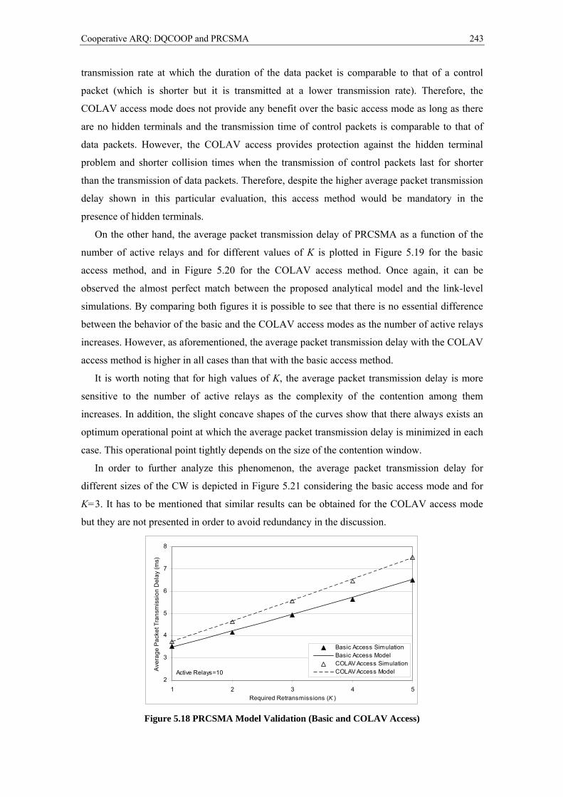
Cooperative ARQ: DQCOOP and PRCSMA 243
transmission rate at which the duration of the data packet is comparable to that of a control
packet (which is shorter but it is transmitted at a lower transmission rate). Therefore, the
COLAV access mode does not provide any benefit over the basic access mode as long as there
are no hidden terminals and the transmission time of control packets is comparable to that of
data packets. However, the COLAV access provides protection against the hidden terminal
problem and shorter collision times when the transmission of control packets last for shorter
than the transmission of data packets. Therefore, despite the higher average packet transmission
delay shown in this particular evaluation, this access method would be mandatory in the
presence of hidden terminals.
On the other hand, the average packet transmission delay of PRCSMA as a function of the
number of active relays and for different values of K is plotted in Figure 5.19 for the basic
access method, and in Figure 5.20 for the COLAV access method. Once again, it can be
observed the almost perfect match between the proposed analytical model and the link-level
simulations. By comparing both figures it is possible to see that there is no essential difference
between the behavior of the basic and the COLAV access modes as the number of active relays
increases. However, as aforementioned, the average packet transmission delay with the COLAV
access method is higher in all cases than that with the basic access method.
It is worth noting that for high values of K, the average packet transmission delay is more
sensitive to the number of active relays as the complexity of the contention among them
increases. In addition, the slight concave shapes of the curves show that there always exists an
optimum operational point at which the average packet transmission delay is minimized in each
case. This operational point tightly depends on the size of the contention window.
In order to further analyze this phenomenon, the average packet transmission delay for
different sizes of the CW is depicted in Figure 5.21 considering the basic access mode and for
K=3. It has to be mentioned that similar results can be obtained for the COLAV access mode
but they are not presented in order to avoid redundancy in the discussion.
2
3
4
5
6
7
8
1 2 3 4 5
Required Retransmissions (K )
Ave
rag
e P
ack
et T
ran
smis
sio
n D
ela
y (m
s)
Basic Access SimulationBasic Access ModelCOLAV Access SimulationCOLAV Access ModelActive Relays=10
Figure 5.18 PRCSMA Model Validation (Basic and COLAV Access)
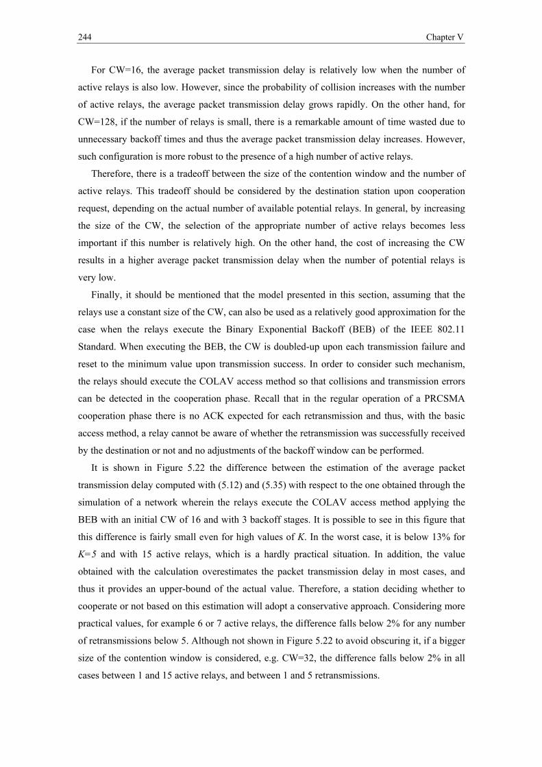
Chapter V
244
For CW=16, the average packet transmission delay is relatively low when the number of
active relays is also low. However, since the probability of collision increases with the number
of active relays, the average packet transmission delay grows rapidly. On the other hand, for
CW=128, if the number of relays is small, there is a remarkable amount of time wasted due to
unnecessary backoff times and thus the average packet transmission delay increases. However,
such configuration is more robust to the presence of a high number of active relays.
Therefore, there is a tradeoff between the size of the contention window and the number of
active relays. This tradeoff should be considered by the destination station upon cooperation
request, depending on the actual number of available potential relays. In general, by increasing
the size of the CW, the selection of the appropriate number of active relays becomes less
important if this number is relatively high. On the other hand, the cost of increasing the CW
results in a higher average packet transmission delay when the number of potential relays is
very low.
Finally, it should be mentioned that the model presented in this section, assuming that the
relays use a constant size of the CW, can also be used as a relatively good approximation for the
case when the relays execute the Binary Exponential Backoff (BEB) of the IEEE 802.11
Standard. When executing the BEB, the CW is doubled-up upon each transmission failure and
reset to the minimum value upon transmission success. In order to consider such mechanism,
the relays should execute the COLAV access method so that collisions and transmission errors
can be detected in the cooperation phase. Recall that in the regular operation of a PRCSMA
cooperation phase there is no ACK expected for each retransmission and thus, with the basic
access method, a relay cannot be aware of whether the retransmission was successfully received
by the destination or not and no adjustments of the backoff window can be performed.
It is shown in Figure 5.22 the difference between the estimation of the average packet
transmission delay computed with (5.12) and (5.35) with respect to the one obtained through the
simulation of a network wherein the relays execute the COLAV access method applying the
BEB with an initial CW of 16 and with 3 backoff stages. It is possible to see in this figure that
this difference is fairly small even for high values of K. In the worst case, it is below 13% for
K=5 and with 15 active relays, which is a hardly practical situation. In addition, the value
obtained with the calculation overestimates the packet transmission delay in most cases, and
thus it provides an upper-bound of the actual value. Therefore, a station deciding whether to
cooperate or not based on this estimation will adopt a conservative approach. Considering more
practical values, for example 6 or 7 active relays, the difference falls below 2% for any number
of retransmissions below 5. Although not shown in Figure 5.22 to avoid obscuring it, if a bigger
size of the contention window is considered, e.g. CW=32, the difference falls below 2% in all
cases between 1 and 15 active relays, and between 1 and 5 retransmissions.
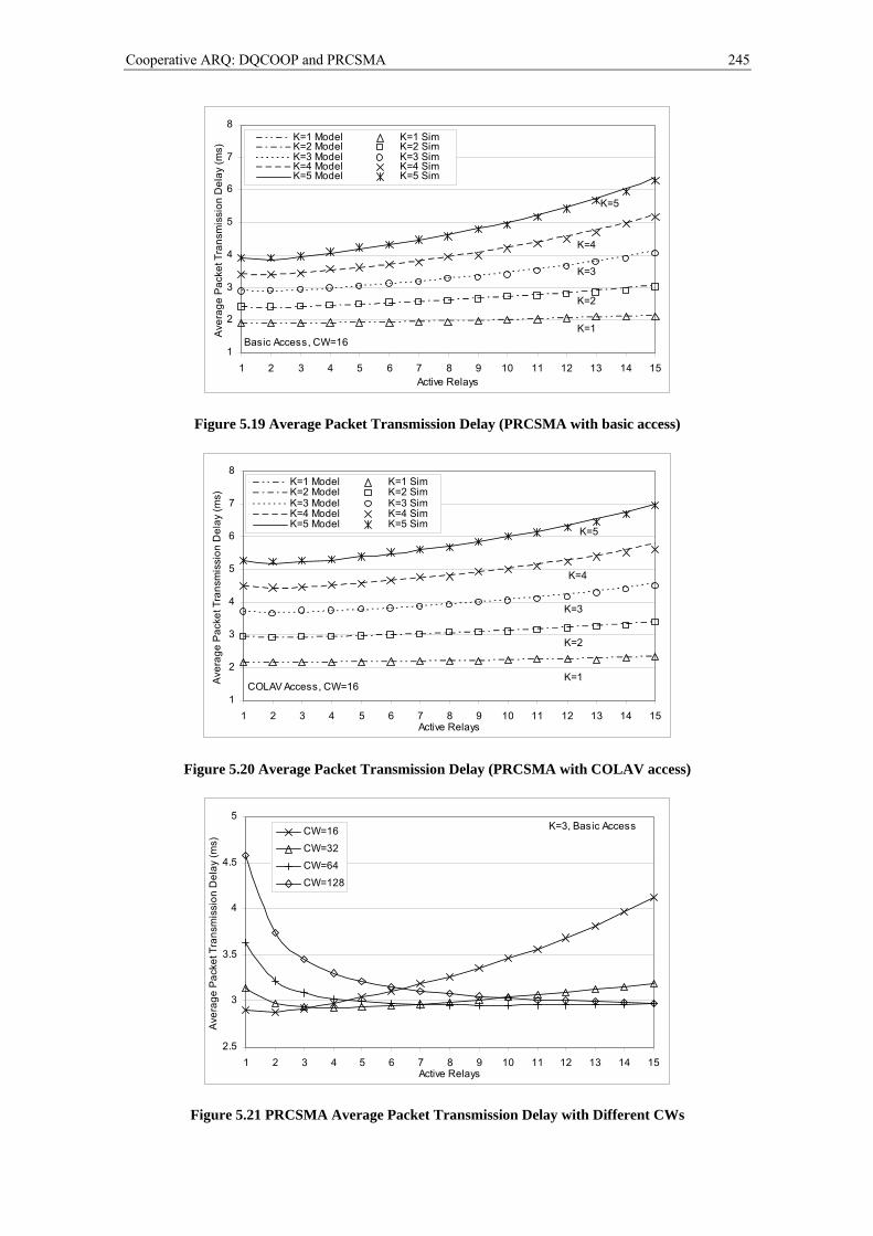
Cooperative ARQ: DQCOOP and PRCSMA 245
1
2
3
4
5
6
7
8
1 2 3 4 5 6 7 8 9 10 11 12 13 14 15Active Relays
Ave
rag
e P
ack
et T
ran
smis
sio
n D
ela
y (m
s)
K=1 Model K=1 SimK=2 Model K=2 SimK=3 Model K=3 SimK=4 Model K=4 SimK=5 Model K=5 Sim
K=1
K=2
K=3
K=4
K=5
Basic Access, CW=16
Figure 5.19 Average Packet Transmission Delay (PRCSMA with basic access)
1
2
3
4
5
6
7
8
1 2 3 4 5 6 7 8 9 10 11 12 13 14 15Active Relays
Ave
rag
e P
ack
et T
ran
smis
sio
n D
ela
y (m
s)
K=1 Model K=1 SimK=2 Model K=2 SimK=3 Model K=3 SimK=4 Model K=4 SimK=5 Model K=5 Sim
COLAV Access, CW=16K=1
K=2
K=3
K=4
K=5
Figure 5.20 Average Packet Transmission Delay (PRCSMA with COLAV access)
2.5
3
3.5
4
4.5
5
1 2 3 4 5 6 7 8 9 10 11 12 13 14 15Active Relays
Ave
rag
e P
ack
et T
ran
smis
sio
n D
ela
y (m
s)
CW=16
CW=32
CW=64
CW=128
K=3, Basic Access
Figure 5.21 PRCSMA Average Packet Transmission Delay with Different CWs
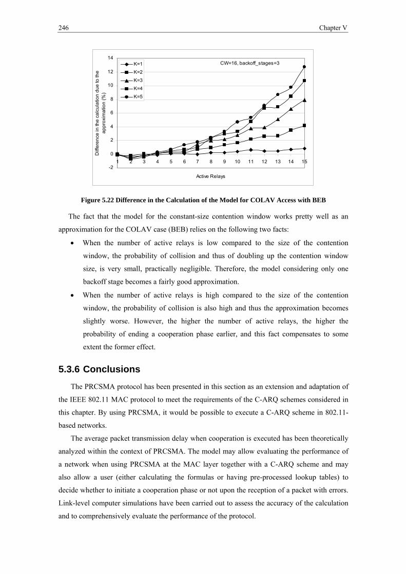
Chapter V
246
-2
0
2
4
6
8
10
12
14
1 2 3 4 5 6 7 8 9 10 11 12 13 14 15
Active Relays
Diff
ere
nce
in th
e c
alc
ula
tion
du
e to
the
a
pp
roxi
ma
tion
(%
)
K=1
K=2
K=3
K=4
K=5
CW=16, backoff_stages=3
Figure 5.22 Difference in the Calculation of the Model for COLAV Access with BEB
The fact that the model for the constant-size contention window works pretty well as an
approximation for the COLAV case (BEB) relies on the following two facts:
When the number of active relays is low compared to the size of the contention
window, the probability of collision and thus of doubling up the contention window
size, is very small, practically negligible. Therefore, the model considering only one
backoff stage becomes a fairly good approximation.
When the number of active relays is high compared to the size of the contention
window, the probability of collision is also high and thus the approximation becomes
slightly worse. However, the higher the number of active relays, the higher the
probability of ending a cooperation phase earlier, and this fact compensates to some
extent the former effect.
5.3.6 Conclusions
The PRCSMA protocol has been presented in this section as an extension and adaptation of
the IEEE 802.11 MAC protocol to meet the requirements of the C-ARQ schemes considered in
this chapter. By using PRCSMA, it would be possible to execute a C-ARQ scheme in 802.11-
based networks.
The average packet transmission delay when cooperation is executed has been theoretically
analyzed within the context of PRCSMA. The model may allow evaluating the performance of
a network when using PRCSMA at the MAC layer together with a C-ARQ scheme and may
also allow a user (either calculating the formulas or having pre-processed lookup tables) to
decide whether to initiate a cooperation phase or not upon the reception of a packet with errors.
Link-level computer simulations have been carried out to assess the accuracy of the calculation
and to comprehensively evaluate the performance of the protocol.
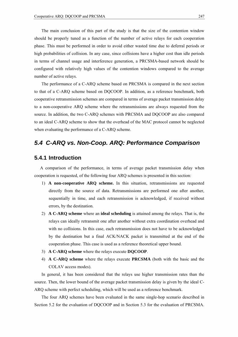
Cooperative ARQ: DQCOOP and PRCSMA 247
The main conclusion of this part of the study is that the size of the contention window
should be properly tuned as a function of the number of active relays for each cooperation
phase. This must be performed in order to avoid either wasted time due to deferral periods or
high probabilities of collision. In any case, since collisions have a higher cost than idle periods
in terms of channel usage and interference generation, a PRCSMA-based network should be
configured with relatively high values of the contention windows compared to the average
number of active relays.
The performance of a C-ARQ scheme based on PRCSMA is compared in the next section
to that of a C-ARQ scheme based on DQCOOP. In addition, as a reference benchmark, both
cooperative retransmission schemes are compared in terms of average packet transmission delay
to a non-cooperative ARQ scheme where the retransmissions are always requested from the
source. In addition, the two C-ARQ schemes with PRCSMA and DQCOOP are also compared
to an ideal C-ARQ scheme to show that the overhead of the MAC protocol cannot be neglected
when evaluating the performance of a C-ARQ scheme.
5.4 C-ARQ vs. Non-Coop. ARQ: Performance Comparison
5.4.1 Introduction
A comparison of the performance, in terms of average packet transmission delay when
cooperation is requested, of the following four ARQ schemes is presented in this section:
1) A non-cooperative ARQ scheme. In this situation, retransmissions are requested
directly from the source of data. Retransmissions are performed one after another,
sequentially in time, and each retransmission is acknowledged, if received without
errors, by the destination.
2) A C-ARQ scheme where an ideal scheduling is attained among the relays. That is, the
relays can ideally retransmit one after another without extra coordination overhead and
with no collisions. In this case, each retransmission does not have to be acknowledged
by the destination but a final ACK/NACK packet is transmitted at the end of the
cooperation phase. This case is used as a reference theoretical upper bound.
3) A C-ARQ scheme where the relays execute DQCOOP.
4) A C-ARQ scheme where the relays execute PRCSMA (both with the basic and the
COLAV access modes).
In general, it has been considered that the relays use higher transmission rates than the
source. Then, the lower bound of the average packet transmission delay is given by the ideal C-
ARQ scheme with perfect scheduling, which will be used as a reference benchmark.
The four ARQ schemes have been evaluated in the same single-hop scenario described in
Section 5.2 for the evaluation of DQCOOP and in Section 5.3 for the evaluation of PRCSMA.

Chapter V
248
In summary, all the data transmissions from source to destination are assumed to have errors,
and thus cooperation is requested by the destination station upon the reception of any packet
received from the source. In addition, and in order to focus on the MAC layer performance, the
channel between the relays and the destination is considered to be error-free. In order to abstract
the results from the specific PHY layer cooperative scheme and the channel conditions, a
constant number of active relays and of required retransmissions (K) has been also considered.
It is worth mentioning that different values of K and the number of active relays have been
simulated to consider different network scenarios. It has to be stressed the fact that it is assumed
in all cases that the relays transmit data at 54 Mbps while the source transmits data at 24 Mbps.
Transmission at the control plane are performed in all cases at 6 Mbps (source and relays).
Finally, and regarding the size of the contention window of PRCSMA, recall that CWmin=16 and
CWmax=128.
The main results of the comparison are presented and discussed in the following section.
5.4.2 Performance Evaluation
The average packet transmission delay when cooperation is requested as a function of the
number of required retransmissions is plotted in Figure 5.23, considering a scenario with 10
active relays.
The curve associated to the performance of DQCOOP is the closest to the theoretical lower-
bound represented by the ideal scheduling in a C-ARQ scheme. In fact, DQCOOP nearly
approaches a perfect TDMA scheduling among the relays, just paying a little price of a certain
constant overhead. This can be seen in the figure, where the curves for DQCOOP and the ideal
scheduling are almost parallel to each other. Therefore a C-ARQ scheme with DQCOOP
outperforms the non-cooperative ARQ in all the considered cases.
On the other hand, it can be observed that when K=1, PRCSMA slightly outperforms
DQCOOP. This is due to that fact that although DQCOOP attains a near-optimum performance,
it requires some start-up time and overhead that may not pay off if the number of required
retransmissions is very low.
When K>1, the performance of the C-ARQ with the basic access model of PRCSMA is
slightly better than that of the non-cooperative ARQ scheme, attaining a lower average packet
transmission delay. However, the C-ARQ scheme with PRCSMA performs worse than the non-
cooperative ARQ when the COLAV access method is executed by the relays and K>1. These
results show that despite the higher transmission rate of the relays, the overhead of the
contention among the relays when executing PRCSMA may compromise the benefits of
cooperation.
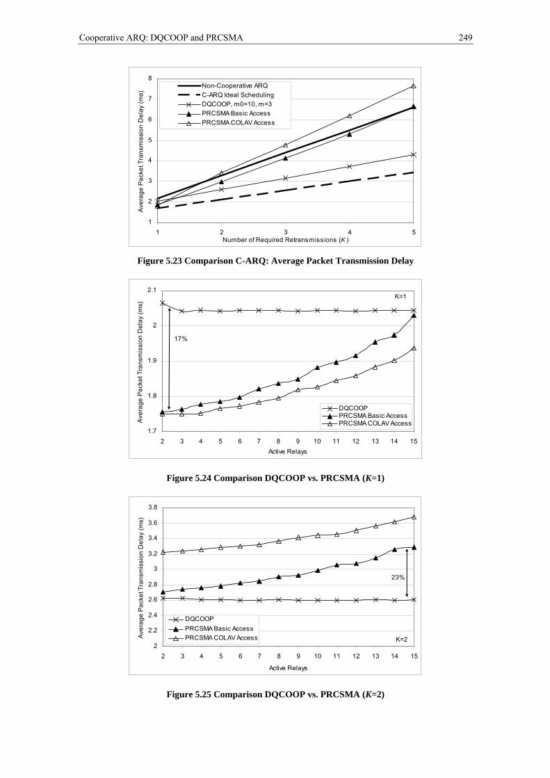
Cooperative ARQ: DQCOOP and PRCSMA 249
1
2
3
4
5
6
7
8
1 2 3 4 5Number of Required Retransmissions (K )
Ave
rag
e P
ack
et T
ran
smis
sio
n D
ela
y (m
s)
Non-Cooperative ARQ
C-ARQ Ideal Scheduling
DQCOOP, m0=10, m=3
PRCSMA Basic Access
PRCSMA COLAV Access
Figure 5.23 Comparison C-ARQ: Average Packet Transmission Delay
1.7
1.8
1.9
2
2.1
2 3 4 5 6 7 8 9 10 11 12 13 14 15
Active Relays
Ave
rag
e P
ack
et T
ran
smis
sio
n D
ela
y (m
s)
DQCOOPPRCSMA Basic AccessPRCSMA COLAV Access
K=1
17%
Figure 5.24 Comparison DQCOOP vs. PRCSMA (K=1)
2
2.2
2.4
2.6
2.8
3
3.2
3.4
3.6
3.8
2 3 4 5 6 7 8 9 10 11 12 13 14 15
Active Relays
Ave
rag
e P
ack
et T
ran
smis
sio
n D
ela
y (m
s)
DQCOOP
PRCSMA Basic Access
PRCSMA COLAV Access K=2
23%
Figure 5.25 Comparison DQCOOP vs. PRCSMA (K=2)
Chapter V
250
This is an extremely important conclusion; ignoring or idealizing the contention
(coordination) among the relays can lead to wrong conclusions regarding the efficiency of
cooperative schemes.
PRCSMA is a completely random access protocol and thus it outperforms DQCOOP when
either the number of active relays is very low or when the value of K is very low. That is,
whenever the (cooperative) traffic is low, in fact, any random access MAC protocol may
operate quite well. In order to evaluate the impact of the number of active relays on the
performance of both protocols, the average packet transmission delay when cooperation is
required is plotted in Figure 5.24 and Figure 5.25 for K=1 and K=2, respectively. It is
interesting to infer from these plots that the performance of PRCSMA is strongly dependent on
the number of active relays. On the other hand, DQCOOP performs almost constantly and
independently of the number of active relays. This is a key feature of DQCOOP, since it loosens
the requirement of selecting the optimum number of active relays to help in a cooperation
phase.
As it was mentioned before, the plots show that, for a low number of active relays and for a
low number of required retransmissions, PRCSMA outperforms DQCOOP. However, the
performance of DQCOOP is less dependent on the configuration of the cooperative scheme and
then it can be said that it outperforms PRCSMA in general cases.
5.4.3 Conclusions
The main conclusions of the comparison between non-cooperative ARQ and C-ARQ
schemes with DQCOOP and PRCSMA can be briefly summarized in two key points:
1) The actual contention among the relays in C-ARQ schemes cannot be idealized when
evaluating their performance. As either the number of potential helpers for a failed
communication or the number of required retransmissions grows, the cost of coordination
among the relays also increases. Therefore, although from a PHY point of view a greater
number of relays and retransmissions may lead to higher diversity gain, the contention at
the MAC layer can compromise the benefits of cooperation. Obviously, the use of
frequency or code division in the transmissions of the relays can solve this problem.
However, the complexity associated to these solutions may make them unfeasible for
current wireless devices.
2) PRCSMA is a contention-based MAC protocol. Therefore, although its performance is high
for low number of active relays, it is also strongly dependent on the number of active relays,
the size of the contention window, and the total amount of required retransmissions upon
error. DQCOOP, on the other hand, is quite efficient when either the number of active
relays or the number of required retransmissions is high, since it has a small overhead to set
Cooperative ARQ: DQCOOP and PRCSMA 251
a virtual perfect TDMA scheduling among the relays. In addition, its performance is less
sensitive to the network configuration and size.
To conclude the chapter, in the next section, the performance of a case study network where
a C-ARQ scheme is executed using either DQCOOP or PRCSMA is analyzed. The impairments
of the radio channel are analytically modeled and a closed expression to compute the throughput
of a network is obtained when any of the four considered ARQ schemes is used.
5.5 Case Study: Rooftop AP Network with C-ARQ
5.5.1 Introduction
In the previous sections, the operation of different C-ARQ schemes in wireless networks
have been described, arguing that they can effectively improve the performance of the
communications. Two novel MAC protocols to coordinate the retransmissions from the time-
orthogonal relays in a fully distributed manner, namely DQCOOP and PRCSMA, have been
designed, analyzed, and evaluated through analytical models and computer simulations. The
first protocol, DQCOOP, is an extension of DQMAN to work in a C-ARQ scheme, and the
latter, PRCSMA, is an extension of the IEEE 802.11 Standard to meet the requirements of the
C-ARQ mechanism. The performances of these two protocols have been analyzed for any
arbitrary number of active relays or number of required retransmissions to decode a failed
packet. In this section, and for the sake of completeness and clarity, the previous analyzes are
applied to a practical scenario, i.e., a case study, giving actual numbers to all the arbitrary
parameters that remained open in the previous sections, namely the number of active relays and
the number of required retransmissions (K).
To do so, the focus is on the performance analysis of the downlink of a rooftop AP network
where a distant source transmits data to a destination which is surrounded by a group of
stations. These stations then can overhear the transmissions from the source to the destination.
Due to the propagation losses and the channel fading, the average SNR in the link from source
to destination is assumed to be low. Therefore, the available effective transmission rate between
source and destination is also low, at least compared to the ones available between the stations
close to the destination and the destination itself. For this reason, retransmissions from the
source are costly in terms of channel usage and a C-ARQ scheme, as the one defined in Section
5.1.1, can help in improving the performance of the network and extending the coverage of the
source to be able to intercommunicate with distant stations.
It is considered that the relays execute a “Decode and Forward” scheme to retransmit when
required. A No Line-Of-Sight (NLOS) block-fading Rayleigh channel is considered. In
particular, block-fading means that the channel quality is assumed to remain constant at least for
the transmission of a whole single data packet.
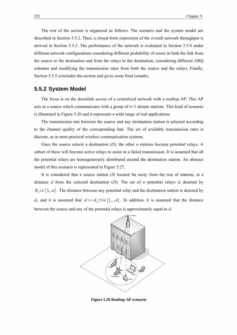
Chapter V
252
The rest of the section is organized as follows. The scenario and the system model are
described in Section 5.5.2. Then, a closed-form expression of the overall network throughput is
derived in Section 5.5.3. The performance of the network is evaluated in Section 5.5.4 under
different network configurations considering different probability of errors in both the link from
the source to the destination and from the relays to the destination, considering different ARQ
schemes and modifying the transmission rates from both the source and the relays. Finally,
Section 5.5.5 concludes the section and gives some final remarks.
5.5.2 System Model
The focus is on the downlink access of a centralized network with a rooftop AP. This AP
acts as a source which communicates with a group of n+1 distant stations. This kind of scenario
is illustrated in Figure 5.26 and it represents a wide range of real applications.
The transmission rate between the source and any destination station is selected according
to the channel quality of the corresponding link. The set of available transmission rates is
discrete, as in most practical wireless communication systems.
Once the source selects a destination (D), the other n stations become potential relays. A
subset of these will become active relays to assist in a failed transmission. It is assumed that all
the potential relays are homogeneously distributed around the destination station. An abstract
model of this scenario is represented in Figure 5.27.
It is considered that a source station (S) located far away from the rest of stations, at a
distance d from the selected destination (D). The set of n potential relays is denoted by
, 1,..iR i n . The distance between any potential relay and the destination station is denoted by
di, and it is assumed that , 1,..,id d i n . In addition, it is assumed that the distance
between the source and any of the potential relays is approximately equal to d. Source
DestinationRelay
Relay
Relay
Figure 5.26 Rooftop AP scenario
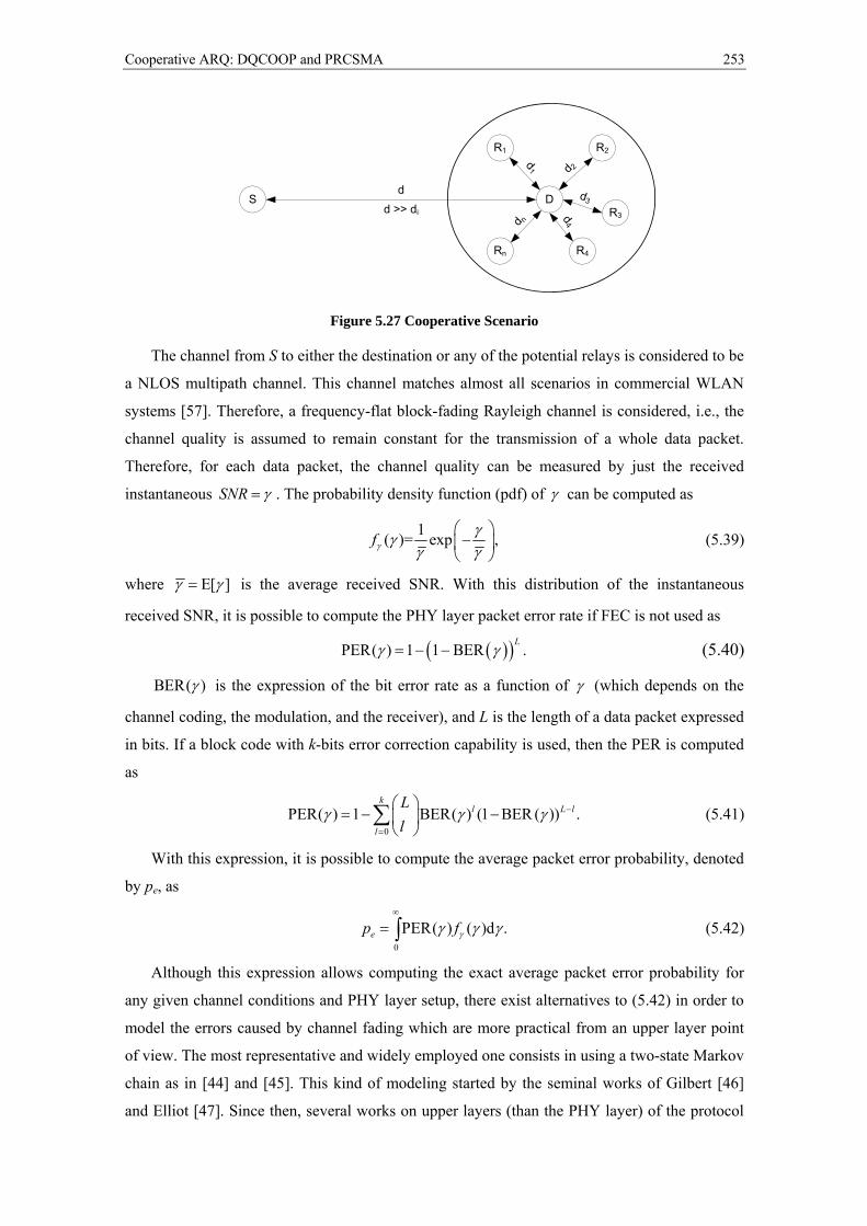
Cooperative ARQ: DQCOOP and PRCSMA 253
S Dd
R1 R2
R3
R4Rn
d2d1
d3
d4d n
d >> di
Figure 5.27 Cooperative Scenario
The channel from S to either the destination or any of the potential relays is considered to be
a NLOS multipath channel. This channel matches almost all scenarios in commercial WLAN
systems [57]. Therefore, a frequency-flat block-fading Rayleigh channel is considered, i.e., the
channel quality is assumed to remain constant for the transmission of a whole data packet.
Therefore, for each data packet, the channel quality can be measured by just the received
instantaneous SNR . The probability density function (pdf) of can be computed as
1
( )= exp ,f
(5.39)
where E[ ] is the average received SNR. With this distribution of the instantaneous
received SNR, it is possible to compute the PHY layer packet error rate if FEC is not used as
PER( ) 1 1 BER .L
(5.40)
BER( ) is the expression of the bit error rate as a function of (which depends on the
channel coding, the modulation, and the receiver), and L is the length of a data packet expressed
in bits. If a block code with k-bits error correction capability is used, then the PER is computed
as
0
PER( ) 1 BER( ) (1 BER ( )) .k
l L l
l
L
l
(5.41)
With this expression, it is possible to compute the average packet error probability, denoted
by pe, as
0
PER( ) ( )d .ep f
(5.42)
Although this expression allows computing the exact average packet error probability for
any given channel conditions and PHY layer setup, there exist alternatives to (5.42) in order to
model the errors caused by channel fading which are more practical from an upper layer point
of view. The most representative and widely employed one consists in using a two-state Markov
chain as in [44] and [45]. This kind of modeling started by the seminal works of Gilbert [46]
and Elliot [47]. Since then, several works on upper layers (than the PHY layer) of the protocol
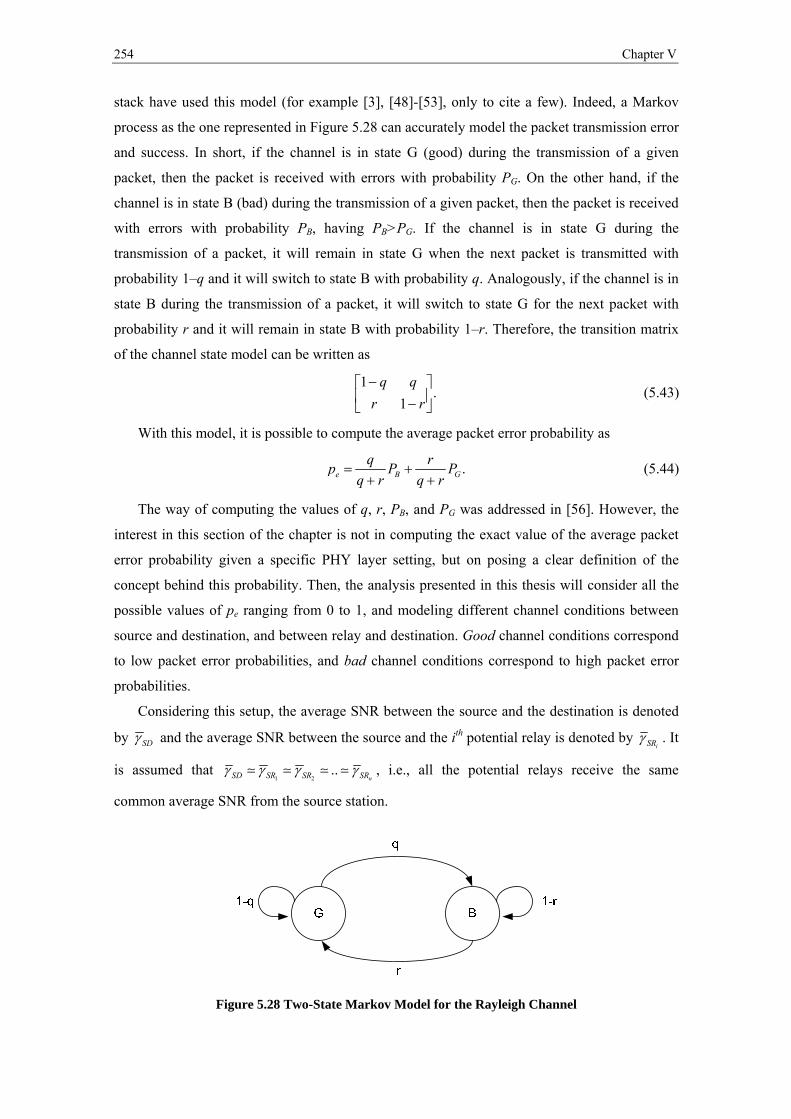
Chapter V
254
stack have used this model (for example [3], [48]-[53], only to cite a few). Indeed, a Markov
process as the one represented in Figure 5.28 can accurately model the packet transmission error
and success. In short, if the channel is in state G (good) during the transmission of a given
packet, then the packet is received with errors with probability PG. On the other hand, if the
channel is in state B (bad) during the transmission of a given packet, then the packet is received
with errors with probability PB, having PB>PG. If the channel is in state G during the
transmission of a packet, it will remain in state G when the next packet is transmitted with
probability 1–q and it will switch to state B with probability q. Analogously, if the channel is in
state B during the transmission of a packet, it will switch to state G for the next packet with
probability r and it will remain in state B with probability 1–r. Therefore, the transition matrix
of the channel state model can be written as
1
.1
q q
r r
(5.43)
With this model, it is possible to compute the average packet error probability as
.e B G
q rp P P
q r q r
(5.44)
The way of computing the values of q, r, PB, and PG was addressed in [56]. However, the
interest in this section of the chapter is not in computing the exact value of the average packet
error probability given a specific PHY layer setting, but on posing a clear definition of the
concept behind this probability. Then, the analysis presented in this thesis will consider all the
possible values of pe ranging from 0 to 1, and modeling different channel conditions between
source and destination, and between relay and destination. Good channel conditions correspond
to low packet error probabilities, and bad channel conditions correspond to high packet error
probabilities.
Considering this setup, the average SNR between the source and the destination is denoted
by SD and the average SNR between the source and the ith potential relay is denoted by iSR . It
is assumed that 1 2
..nSD SR SR SR , i.e., all the potential relays receive the same
common average SNR from the source station.
Figure 5.28 Two-State Markov Model for the Rayleigh Channel
Cooperative ARQ: DQCOOP and PRCSMA 255
All the relays have a separation with each other such that statistically identical and
independent realizations of the channel can be considered upon transmission from the source.
Note that, for example, in the band of 2.4GHz, the distance between two points where the
autocorrelation of the channel is lower than 10% of the maximum is of 12 cm [5].
Similarly, it is considered that all the channel qualities between the relays and the
destination station are random variables with identically distributed and independent
realizations. The average SNR perceived at the destination for the signal transmitted by the
relay i is denoted by iR D . It is assumed that these values have the same average for all the
relays and this value is denoted by R , and thus 1 2
..D nR R R D R D .
These two average SNRs ( SD and R ) are mapped into two independent average values of
pe, denoted by pSD (from the source to the destination) and pRD (from any relay to the
destination), respectively. In general, pSD>pRD, and thus communication among the destination
stations can be performed at a higher transmission rates compared to these with the source
station. However, in fact this condition is not mandatory, and all possible values of both pSD and
pRD may be considered.
As aforementioned, once the source selects one specific destination station (D), the other n
stations close to D become spontaneous potential relays. The destination station transmits a
CFC packet only when a data packet from the destination is received with errors. The particular
case wherein those stations which successfully (without errors) receive both the original data
packet from the source and the CFC from the destination station become active relays is
considered in this section. It is assumed that the channel quality between the relays and the
destination station is such that transmissions in the control plane are error-free, and thus the
CFC is received without errors by all the potential relays (recall that control packets are
transmitted at the most robust coding scheme and are very short in length compared to data
packets). Therefore, the interest is on computing the average number of relays that are actually
activated, denoted by E[R], which can be computed, within the context of the considered setup
as
1
r r0 0 0
1 1
0 00 0
1 1
0 0
E[ ] P P
(1 ) (1 )
.
ei
ei ei
ei ei
n n
p ei eieir r
n nr n r r n r
ei ei p ei ei ei ei p ei eir r
ei p ei ei ei p ei ei e
R r R r r R r p f p dp
n nr p p f p dp r p p f p dp
r r
np f p dp n p f p dp np
(5.45)
where pei is the instantaneous value of the packet error probability, fpei(pei) is the pdf of pei. As
the value of SDp becomes higher, there is a non-negligible probability that none of the n
potential relays receive the original packet, and thus no relays are available to cooperate upon
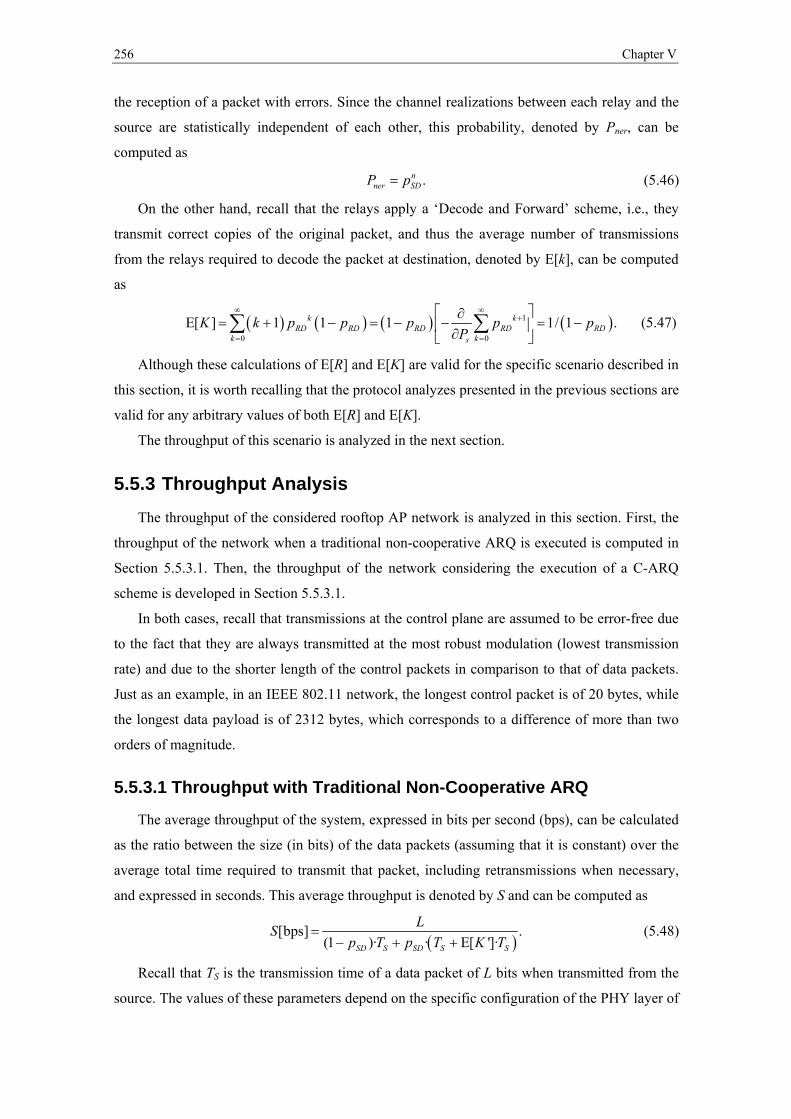
Chapter V
256
the reception of a packet with errors. Since the channel realizations between each relay and the
source are statistically independent of each other, this probability, denoted by Pner, can be
computed as
.nner SDP p (5.46)
On the other hand, recall that the relays apply a ‘Decode and Forward’ scheme, i.e., they
transmit correct copies of the original packet, and thus the average number of transmissions
from the relays required to decode the packet at destination, denoted by E[k], can be computed
as
1
0 0
E[ ] 1 1 1 1/ 1 .k kRD RD RD RD RD
k ks
K k p p p p pP
(5.47)
Although these calculations of E[R] and E[K] are valid for the specific scenario described in
this section, it is worth recalling that the protocol analyzes presented in the previous sections are
valid for any arbitrary values of both E[R] and E[K].
The throughput of this scenario is analyzed in the next section.
5.5.3 Throughput Analysis
The throughput of the considered rooftop AP network is analyzed in this section. First, the
throughput of the network when a traditional non-cooperative ARQ is executed is computed in
Section 5.5.3.1. Then, the throughput of the network considering the execution of a C-ARQ
scheme is developed in Section 5.5.3.1.
In both cases, recall that transmissions at the control plane are assumed to be error-free due
to the fact that they are always transmitted at the most robust modulation (lowest transmission
rate) and due to the shorter length of the control packets in comparison to that of data packets.
Just as an example, in an IEEE 802.11 network, the longest control packet is of 20 bytes, while
the longest data payload is of 2312 bytes, which corresponds to a difference of more than two
orders of magnitude.
5.5.3.1 Throughput with Traditional Non-Cooperative ARQ
The average throughput of the system, expressed in bits per second (bps), can be calculated
as the ratio between the size (in bits) of the data packets (assuming that it is constant) over the
average total time required to transmit that packet, including retransmissions when necessary,
and expressed in seconds. This average throughput is denoted by S and can be computed as
[bps] .(1 )· · E[ ']·SD S SD S S
LS
p T p T K T
(5.48)
Recall that TS is the transmission time of a data packet of L bits when transmitted from the
source. The values of these parameters depend on the specific configuration of the PHY layer of
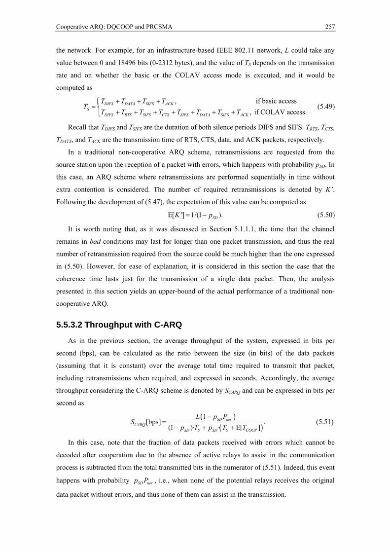
Cooperative ARQ: DQCOOP and PRCSMA 257
the network. For example, for an infrastructure-based IEEE 802.11 network, L could take any
value between 0 and 18496 bits (0-2312 bytes), and the value of TS depends on the transmission
rate and on whether the basic or the COLAV access mode is executed, and it would be
computed as
, if basic access
, if COLAV access.DIFS DATA SIFS ACK
SDIFS RTS SIFS CTS SIFS DATA SIFS ACK
T T T TT
T T T T T T T T
(5.49)
Recall that TDIFS and TSIFS are the duration of both silence periods DIFS and SIFS. TRTS, TCTS,
TDATA, and TACK are the transmission time of RTS, CTS, data, and ACK packets, respectively.
In a traditional non-cooperative ARQ scheme, retransmissions are requested from the
source station upon the reception of a packet with errors, which happens with probability pSD. In
this case, an ARQ scheme where retransmissions are performed sequentially in time without
extra contention is considered. The number of required retransmissions is denoted by K’.
Following the development of (5.47), the expectation of this value can be computed as
E[ '] 1/(1 ).SDK p (5.50)
It is worth noting that, as it was discussed in Section 5.1.1.1, the time that the channel
remains in bad conditions may last for longer than one packet transmission, and thus the real
number of retransmission required from the source could be much higher than the one expressed
in (5.50). However, for ease of explanation, it is considered in this section the case that the
coherence time lasts just for the transmission of a single data packet. Then, the analysis
presented in this section yields an upper-bound of the actual performance of a traditional non-
cooperative ARQ.
5.5.3.2 Throughput with C-ARQ
As in the previous section, the average throughput of the system, expressed in bits per
second (bps), can be calculated as the ratio between the size (in bits) of the data packets
(assuming that it is constant) over the average total time required to transmit that packet,
including retransmissions when required, and expressed in seconds. Accordingly, the average
throughput considering the C-ARQ scheme is denoted by SCARQ and can be expressed in bits per
second as
1
[bps] .(1 )· · E[ ]
SD nerCARQ
SD S SD S COOP
L p PS
p T p T T
(5.51)
In this case, note that the fraction of data packets received with errors which cannot be
decoded after cooperation due to the absence of active relays to assist in the communication
process is subtracted from the total transmitted bits in the numerator of (5.51). Indeed, this event
happens with probability SD nerp P , i.e., when none of the potential relays receives the original
data packet without errors, and thus none of them can assist in the transmission.
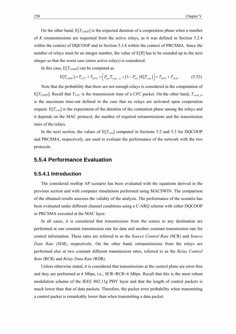
Chapter V
258
On the other hand, E[TCOOP] is the expected duration of a cooperation phase when a number
of K retransmissions are requested from the active relays, as it was defined in Section 5.2.4
within the context of DQCOOP and in Section 5.3.4 within the context of PRCSMA. Since the
number of relays must be an integer number, the value of E[R] has to be rounded up to the next
integer so that the worst case (more active relays) is considered.
In this case, E[TCOOP] can be computed as
_E[ ] 1 E[ ] .COOP CFC SIFS ner coop to ner cont SIFS ACKT T T P T P T T T (5.52)
Note that the probability that there are not enough relays is considered in the computation of
E[TCOOP]. Recall that TCFC is the transmission time of a CFC packet. On the other hand, Tcoop_to
is the maximum time-out defined in the case that no relays are activated upon cooperation
request. E[Tcont] is the expectation of the duration of the contention phase among the relays and
it depends on the MAC protocol, the number of required retransmissions and the transmission
rates of the relays.
In the next section, the values of E[Tcont] computed in Sections 5.2 and 5.3 for DQCOOP
and PRCSMA, respectively, are used to evaluate the performance of the network with the two
protocols.
5.5.4 Performance Evaluation
5.5.4.1 Introduction
The considered rooftop AP scenario has been evaluated with the equations derived in the
previous section and with computer simulations performed using MACSWIN. The comparison
of the obtained results assesses the validity of the analysis. The performance of the scenario has
been evaluated under different channel conditions using a C-ARQ scheme with either DQCOOP
or PRCSMA executed at the MAC layer.
In all cases, it is considered that transmissions from the source to any destination are
performed at one constant transmission rate for data and another constant transmission rate for
control information. These rates are referred to as the Source Control Rate (SCR) and Source
Data Rate (SDR), respectively. On the other hand, retransmissions from the relays are
performed also at two constant different transmission rates, referred to as the Relay Control
Rate (RCR) and Relay Data Rate (RDR).
Unless otherwise stated, it is considered that transmissions at the control plane are error-free
and they are performed at 6 Mbps, i.e., SCR=RCR=6 Mbps. Recall that this is the most robust
modulation scheme of the IEEE 802.11g PHY layer and that the length of control packets is
much lower than that of data packets. Therefore, the packet error probability when transmitting
a control packet is remarkably lower than when transmitting a data packet.
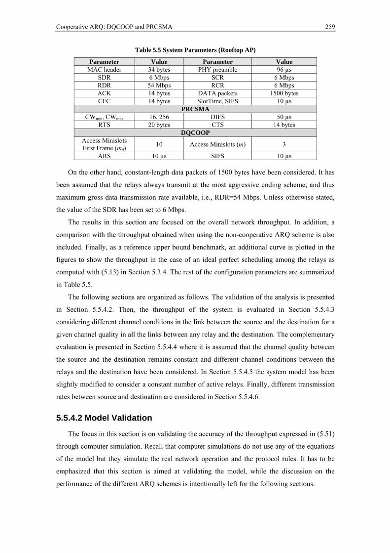
Cooperative ARQ: DQCOOP and PRCSMA 259
Table 5.5 System Parameters (Rooftop AP)
Parameter Value Parameter Value MAC header 34 bytes PHY preamble 96 µs
SDR 6 Mbps SCR 6 Mbps RDR 54 Mbps RCR 6 Mbps ACK 14 bytes DATA packets 1500 bytes CFC 14 bytes SlotTime, SIFS 10 µs
PRCSMA CWmin, CWmax 16, 256 DIFS 50 µs
RTS 20 bytes CTS 14 bytes DQCOOP
Access Minislots First Frame (m0)
10 Access Minislots (m) 3
ARS 10 µs SIFS 10 µs
On the other hand, constant-length data packets of 1500 bytes have been considered. It has
been assumed that the relays always transmit at the most aggressive coding scheme, and thus
maximum gross data transmission rate available, i.e., RDR=54 Mbps. Unless otherwise stated,
the value of the SDR has been set to 6 Mbps.
The results in this section are focused on the overall network throughput. In addition, a
comparison with the throughput obtained when using the non-cooperative ARQ scheme is also
included. Finally, as a reference upper bound benchmark, an additional curve is plotted in the
figures to show the throughput in the case of an ideal perfect scheduling among the relays as
computed with (5.13) in Section 5.3.4. The rest of the configuration parameters are summarized
in Table 5.5.
The following sections are organized as follows. The validation of the analysis is presented
in Section 5.5.4.2. Then, the throughput of the system is evaluated in Section 5.5.4.3
considering different channel conditions in the link between the source and the destination for a
given channel quality in all the links between any relay and the destination. The complementary
evaluation is presented in Section 5.5.4.4 where it is assumed that the channel quality between
the source and the destination remains constant and different channel conditions between the
relays and the destination have been considered. In Section 5.5.4.5 the system model has been
slightly modified to consider a constant number of active relays. Finally, different transmission
rates between source and destination are considered in Section 5.5.4.6.
5.5.4.2 Model Validation
The focus in this section is on validating the accuracy of the throughput expressed in (5.51)
through computer simulation. Recall that computer simulations do not use any of the equations
of the model but they simulate the real network operation and the protocol rules. It has to be
emphasized that this section is aimed at validating the model, while the discussion on the
performance of the different ARQ schemes is intentionally left for the following sections.
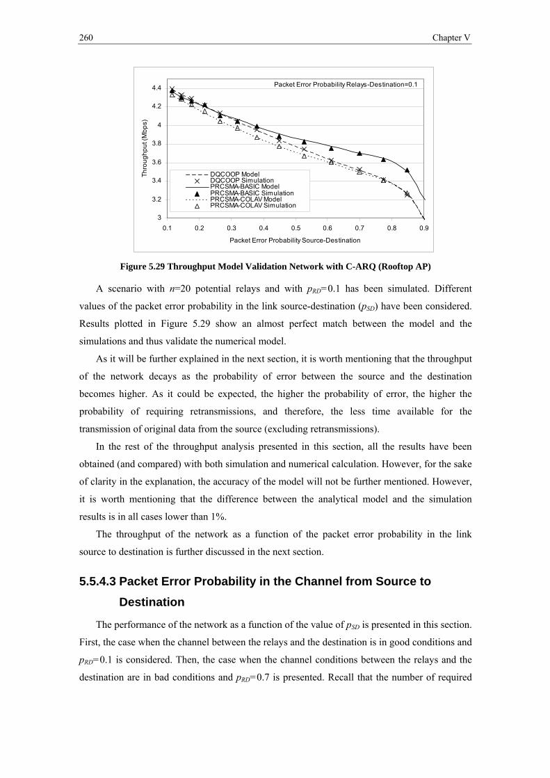
Chapter V
260
3
3.2
3.4
3.6
3.8
4
4.2
4.4
0.1 0.2 0.3 0.4 0.5 0.6 0.7 0.8 0.9
Packet Error Probability Source-Destination
Th
rou
gh
pu
t (M
bp
s)
DQCOOP ModelDQCOOP SimulationPRCSMA-BASIC ModelPRCSMA-BASIC SimulationPRCSMA-COLAV ModelPRCSMA-COLAV Simulation
Packet Error Probability Relays-Destination=0.1
Figure 5.29 Throughput Model Validation Network with C-ARQ (Rooftop AP)
A scenario with n=20 potential relays and with pRD=0.1 has been simulated. Different
values of the packet error probability in the link source-destination (pSD) have been considered.
Results plotted in Figure 5.29 show an almost perfect match between the model and the
simulations and thus validate the numerical model.
As it will be further explained in the next section, it is worth mentioning that the throughput
of the network decays as the probability of error between the source and the destination
becomes higher. As it could be expected, the higher the probability of error, the higher the
probability of requiring retransmissions, and therefore, the less time available for the
transmission of original data from the source (excluding retransmissions).
In the rest of the throughput analysis presented in this section, all the results have been
obtained (and compared) with both simulation and numerical calculation. However, for the sake
of clarity in the explanation, the accuracy of the model will not be further mentioned. However,
it is worth mentioning that the difference between the analytical model and the simulation
results is in all cases lower than 1%.
The throughput of the network as a function of the packet error probability in the link
source to destination is further discussed in the next section.
5.5.4.3 Packet Error Probability in the Channel from Source to
Destination
The performance of the network as a function of the value of pSD is presented in this section.
First, the case when the channel between the relays and the destination is in good conditions and
pRD=0.1 is considered. Then, the case when the channel conditions between the relays and the
destination are in bad conditions and pRD=0.7 is presented. Recall that the number of required
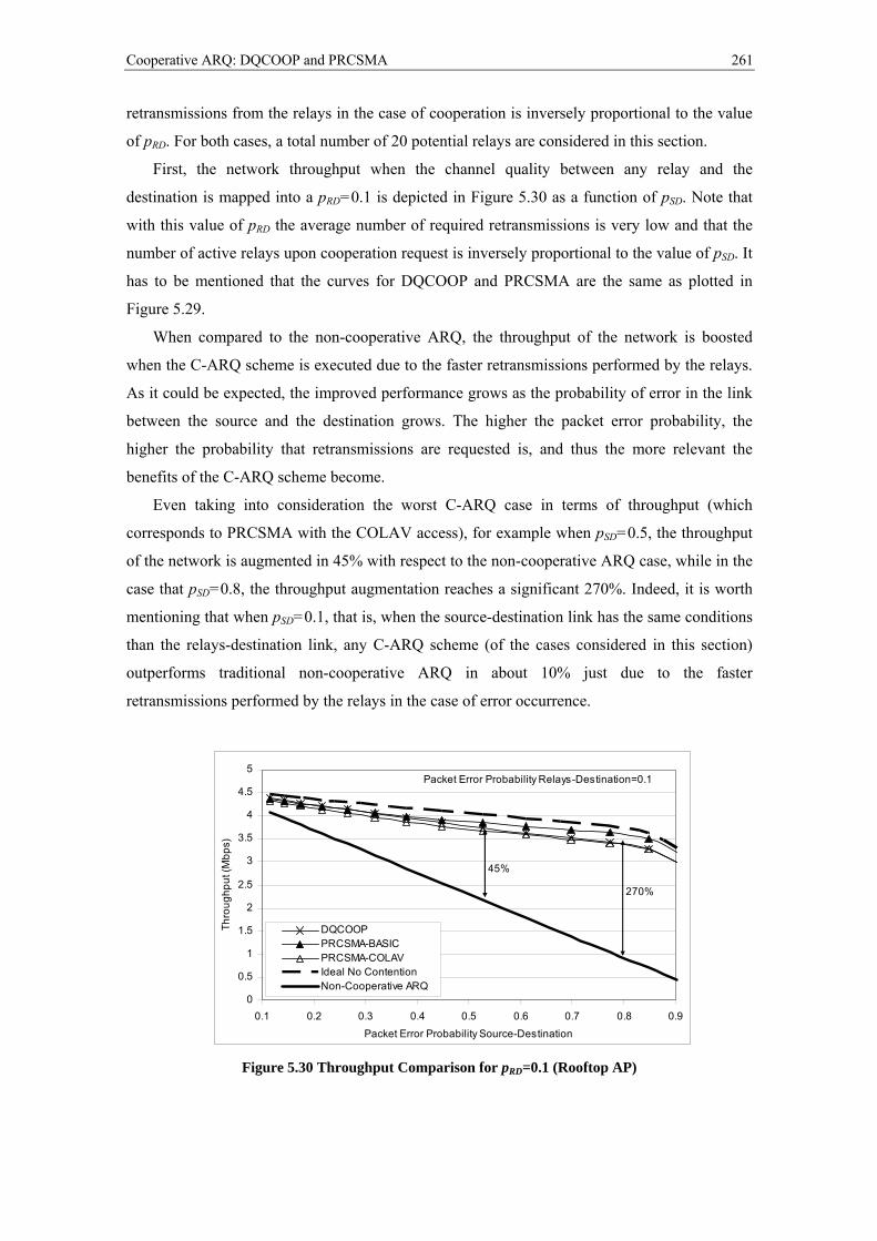
Cooperative ARQ: DQCOOP and PRCSMA 261
retransmissions from the relays in the case of cooperation is inversely proportional to the value
of pRD. For both cases, a total number of 20 potential relays are considered in this section.
First, the network throughput when the channel quality between any relay and the
destination is mapped into a pRD=0.1 is depicted in Figure 5.30 as a function of pSD. Note that
with this value of pRD the average number of required retransmissions is very low and that the
number of active relays upon cooperation request is inversely proportional to the value of pSD. It
has to be mentioned that the curves for DQCOOP and PRCSMA are the same as plotted in
Figure 5.29.
When compared to the non-cooperative ARQ, the throughput of the network is boosted
when the C-ARQ scheme is executed due to the faster retransmissions performed by the relays.
As it could be expected, the improved performance grows as the probability of error in the link
between the source and the destination grows. The higher the packet error probability, the
higher the probability that retransmissions are requested is, and thus the more relevant the
benefits of the C-ARQ scheme become.
Even taking into consideration the worst C-ARQ case in terms of throughput (which
corresponds to PRCSMA with the COLAV access), for example when pSD=0.5, the throughput
of the network is augmented in 45% with respect to the non-cooperative ARQ case, while in the
case that pSD=0.8, the throughput augmentation reaches a significant 270%. Indeed, it is worth
mentioning that when pSD=0.1, that is, when the source-destination link has the same conditions
than the relays-destination link, any C-ARQ scheme (of the cases considered in this section)
outperforms traditional non-cooperative ARQ in about 10% just due to the faster
retransmissions performed by the relays in the case of error occurrence.
0
0.5
1
1.5
2
2.5
3
3.5
4
4.5
5
0.1 0.2 0.3 0.4 0.5 0.6 0.7 0.8 0.9
Packet Error Probability Source-Destination
Th
rou
gh
pu
t (M
bp
s)
DQCOOPPRCSMA-BASICPRCSMA-COLAVIdeal No ContentionNon-Cooperative ARQ
Packet Error Probability Relays-Destination=0.1
45%
270%
Figure 5.30 Throughput Comparison for pRD=0.1 (Rooftop AP)
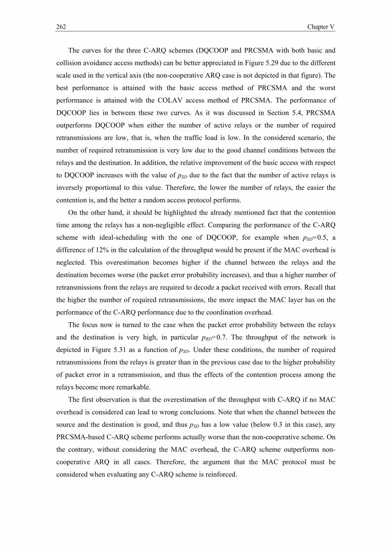
Chapter V
262
The curves for the three C-ARQ schemes (DQCOOP and PRCSMA with both basic and
collision avoidance access methods) can be better appreciated in Figure 5.29 due to the different
scale used in the vertical axis (the non-cooperative ARQ case is not depicted in that figure). The
best performance is attained with the basic access method of PRCSMA and the worst
performance is attained with the COLAV access method of PRCSMA. The performance of
DQCOOP lies in between these two curves. As it was discussed in Section 5.4, PRCSMA
outperforms DQCOOP when either the number of active relays or the number of required
retransmissions are low, that is, when the traffic load is low. In the considered scenario, the
number of required retransmission is very low due to the good channel conditions between the
relays and the destination. In addition, the relative improvement of the basic access with respect
to DQCOOP increases with the value of pSD due to the fact that the number of active relays is
inversely proportional to this value. Therefore, the lower the number of relays, the easier the
contention is, and the better a random access protocol performs.
On the other hand, it should be highlighted the already mentioned fact that the contention
time among the relays has a non-negligible effect. Comparing the performance of the C-ARQ
scheme with ideal-scheduling with the one of DQCOOP, for example when pSD=0.5, a
difference of 12% in the calculation of the throughput would be present if the MAC overhead is
neglected. This overestimation becomes higher if the channel between the relays and the
destination becomes worse (the packet error probability increases), and thus a higher number of
retransmissions from the relays are required to decode a packet received with errors. Recall that
the higher the number of required retransmissions, the more impact the MAC layer has on the
performance of the C-ARQ performance due to the coordination overhead.
The focus now is turned to the case when the packet error probability between the relays
and the destination is very high, in particular pRD=0.7. The throughput of the network is
depicted in Figure 5.31 as a function of pSD. Under these conditions, the number of required
retransmissions from the relays is greater than in the previous case due to the higher probability
of packet error in a retransmission, and thus the effects of the contention process among the
relays become more remarkable.
The first observation is that the overestimation of the throughput with C-ARQ if no MAC
overhead is considered can lead to wrong conclusions. Note that when the channel between the
source and the destination is good, and thus pSD has a low value (below 0.3 in this case), any
PRCSMA-based C-ARQ scheme performs actually worse than the non-cooperative scheme. On
the contrary, without considering the MAC overhead, the C-ARQ scheme outperforms non-
cooperative ARQ in all cases. Therefore, the argument that the MAC protocol must be
considered when evaluating any C-ARQ scheme is reinforced.
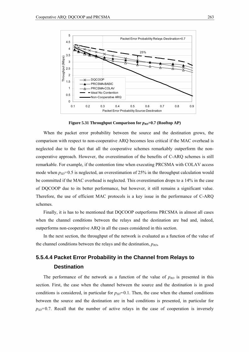
Cooperative ARQ: DQCOOP and PRCSMA 263
0
0.5
1
1.5
2
2.5
3
3.5
4
4.5
5
0.1 0.2 0.3 0.4 0.5 0.6 0.7 0.8 0.9
Packet Error Probability Source-Destination
Th
rou
gh
pu
t (M
bp
s)
DQCOOP
PRCSMA-BASIC
PRCSMA-COLAV
Ideal No Contention
Non-Cooperative ARQ
Packet Error Probability Relays-Destination=0.7
25%
Figure 5.31 Throughput Comparison for pRD=0.7 (Rooftop AP)
When the packet error probability between the source and the destination grows, the
comparison with respect to non-cooperative ARQ becomes less critical if the MAC overhead is
neglected due to the fact that all the cooperative schemes remarkably outperform the non-
cooperative approach. However, the overestimation of the benefits of C-ARQ schemes is still
remarkable. For example, if the contention time when executing PRCSMA with COLAV access
mode when pSD=0.5 is neglected, an overestimation of 25% in the throughput calculation would
be committed if the MAC overhead is neglected. This overestimation drops to a 14% in the case
of DQCOOP due to its better performance, but however, it still remains a significant value.
Therefore, the use of efficient MAC protocols is a key issue in the performance of C-ARQ
schemes.
Finally, it is has to be mentioned that DQCOOP outperforms PRCSMA in almost all cases
when the channel conditions between the relays and the destination are bad and, indeed,
outperforms non-cooperative ARQ in all the cases considered in this section.
In the next section, the throughput of the network is evaluated as a function of the value of
the channel conditions between the relays and the destination, pRD,
5.5.4.4 Packet Error Probability in the Channel from Relays to
Destination
The performance of the network as a function of the value of pRD is presented in this
section. First, the case when the channel between the source and the destination is in good
conditions is considered, in particular for pSD=0.1. Then, the case when the channel conditions
between the source and the destination are in bad conditions is presented, in particular for
pSD=0.7. Recall that the number of active relays in the case of cooperation is inversely
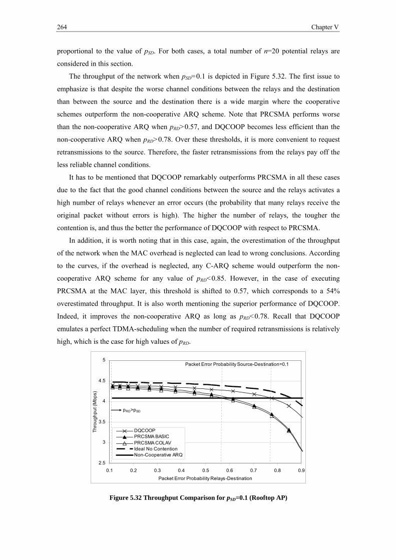
Chapter V
264
proportional to the value of pSD. For both cases, a total number of n=20 potential relays are
considered in this section.
The throughput of the network when pSD=0.1 is depicted in Figure 5.32. The first issue to
emphasize is that despite the worse channel conditions between the relays and the destination
than between the source and the destination there is a wide margin where the cooperative
schemes outperform the non-cooperative ARQ scheme. Note that PRCSMA performs worse
than the non-cooperative ARQ when pRD>0.57, and DQCOOP becomes less efficient than the
non-cooperative ARQ when pRD>0.78. Over these thresholds, it is more convenient to request
retransmissions to the source. Therefore, the faster retransmissions from the relays pay off the
less reliable channel conditions.
It has to be mentioned that DQCOOP remarkably outperforms PRCSMA in all these cases
due to the fact that the good channel conditions between the source and the relays activates a
high number of relays whenever an error occurs (the probability that many relays receive the
original packet without errors is high). The higher the number of relays, the tougher the
contention is, and thus the better the performance of DQCOOP with respect to PRCSMA.
In addition, it is worth noting that in this case, again, the overestimation of the throughput
of the network when the MAC overhead is neglected can lead to wrong conclusions. According
to the curves, if the overhead is neglected, any C-ARQ scheme would outperform the non-
cooperative ARQ scheme for any value of pRD<0.85. However, in the case of executing
PRCSMA at the MAC layer, this threshold is shifted to 0.57, which corresponds to a 54%
overestimated throughput. It is also worth mentioning the superior performance of DQCOOP.
Indeed, it improves the non-cooperative ARQ as long as pRD<0.78. Recall that DQCOOP
emulates a perfect TDMA-scheduling when the number of required retransmissions is relatively
high, which is the case for high values of pRD.
2.5
3
3.5
4
4.5
5
0.1 0.2 0.3 0.4 0.5 0.6 0.7 0.8 0.9
Packet Error Probability Relays-Destination
Th
rou
gh
pu
t (M
bp
s)
DQCOOPPRCSMA BASICPRCSMA COLAVIdeal No ContentionNon-Cooperative ARQ
pRD>pSD
Packet Error Probability Source-Destination=0.1
Figure 5.32 Throughput Comparison for pSD=0.1 (Rooftop AP)
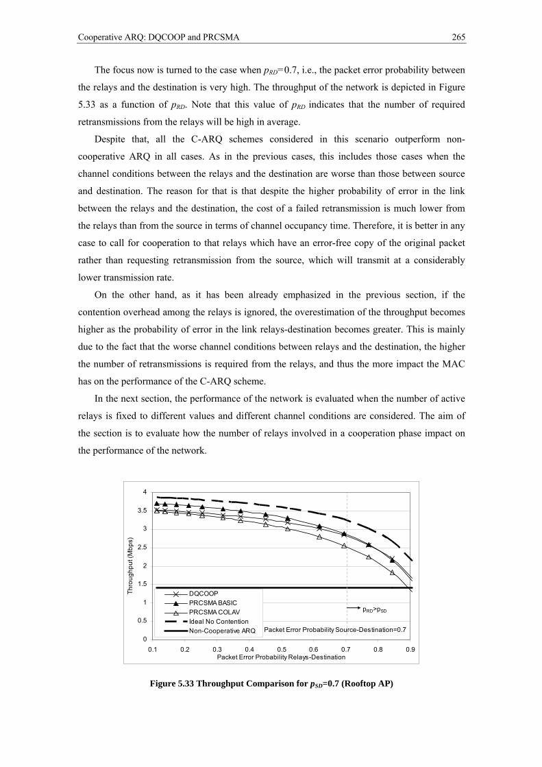
Cooperative ARQ: DQCOOP and PRCSMA 265
The focus now is turned to the case when pRD=0.7, i.e., the packet error probability between
the relays and the destination is very high. The throughput of the network is depicted in Figure
5.33 as a function of pRD. Note that this value of pRD indicates that the number of required
retransmissions from the relays will be high in average.
Despite that, all the C-ARQ schemes considered in this scenario outperform non-
cooperative ARQ in all cases. As in the previous cases, this includes those cases when the
channel conditions between the relays and the destination are worse than those between source
and destination. The reason for that is that despite the higher probability of error in the link
between the relays and the destination, the cost of a failed retransmission is much lower from
the relays than from the source in terms of channel occupancy time. Therefore, it is better in any
case to call for cooperation to that relays which have an error-free copy of the original packet
rather than requesting retransmission from the source, which will transmit at a considerably
lower transmission rate.
On the other hand, as it has been already emphasized in the previous section, if the
contention overhead among the relays is ignored, the overestimation of the throughput becomes
higher as the probability of error in the link relays-destination becomes greater. This is mainly
due to the fact that the worse channel conditions between relays and the destination, the higher
the number of retransmissions is required from the relays, and thus the more impact the MAC
has on the performance of the C-ARQ scheme.
In the next section, the performance of the network is evaluated when the number of active
relays is fixed to different values and different channel conditions are considered. The aim of
the section is to evaluate how the number of relays involved in a cooperation phase impact on
the performance of the network.
0
0.5
1
1.5
2
2.5
3
3.5
4
0.1 0.2 0.3 0.4 0.5 0.6 0.7 0.8 0.9Packet Error Probability Relays-Destination
Th
rou
gh
pu
t (M
bp
s)
DQCOOP
PRCSMA BASIC
PRCSMA COLAV
Ideal No Contention
Non-Cooperative ARQ Packet Error Probability Source-Destination=0.7
pRD>pSD
Figure 5.33 Throughput Comparison for pSD=0.7 (Rooftop AP)
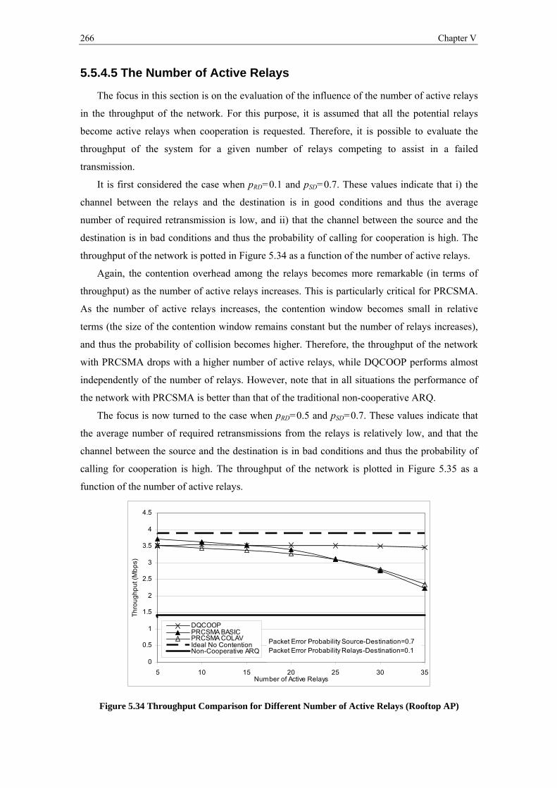
Chapter V
266
5.5.4.5 The Number of Active Relays
The focus in this section is on the evaluation of the influence of the number of active relays
in the throughput of the network. For this purpose, it is assumed that all the potential relays
become active relays when cooperation is requested. Therefore, it is possible to evaluate the
throughput of the system for a given number of relays competing to assist in a failed
transmission.
It is first considered the case when pRD=0.1 and pSD=0.7. These values indicate that i) the
channel between the relays and the destination is in good conditions and thus the average
number of required retransmission is low, and ii) that the channel between the source and the
destination is in bad conditions and thus the probability of calling for cooperation is high. The
throughput of the network is potted in Figure 5.34 as a function of the number of active relays.
Again, the contention overhead among the relays becomes more remarkable (in terms of
throughput) as the number of active relays increases. This is particularly critical for PRCSMA.
As the number of active relays increases, the contention window becomes small in relative
terms (the size of the contention window remains constant but the number of relays increases),
and thus the probability of collision becomes higher. Therefore, the throughput of the network
with PRCSMA drops with a higher number of active relays, while DQCOOP performs almost
independently of the number of relays. However, note that in all situations the performance of
the network with PRCSMA is better than that of the traditional non-cooperative ARQ.
The focus is now turned to the case when pRD=0.5 and pSD=0.7. These values indicate that
the average number of required retransmissions from the relays is relatively low, and that the
channel between the source and the destination is in bad conditions and thus the probability of
calling for cooperation is high. The throughput of the network is plotted in Figure 5.35 as a
function of the number of active relays.
0
0.5
1
1.5
2
2.5
3
3.5
4
4.5
5 10 15 20 25 30 35Number of Active Relays
Th
rou
gh
pu
t (M
bp
s)
DQCOOPPRCSMA BASICPRCSMA COLAVIdeal No ContentionNon-Cooperative ARQ
Packet Error Probability Source-Destination=0.7 Packet Error Probability Relays-Destination=0.1
Figure 5.34 Throughput Comparison for Different Number of Active Relays (Rooftop AP)
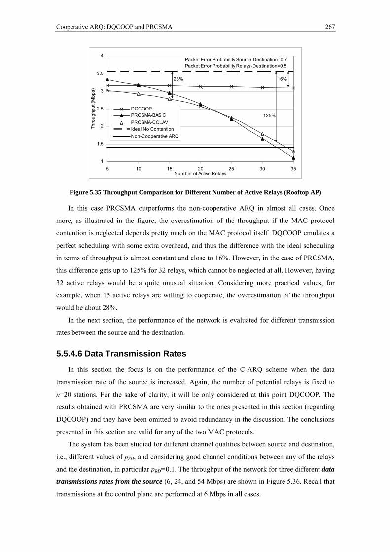
Cooperative ARQ: DQCOOP and PRCSMA 267
1
1.5
2
2.5
3
3.5
4
5 10 15 20 25 30 35Number of Active Relays
Th
rou
gh
pu
t (M
bp
s)
DQCOOP
PRCSMA-BASIC
PRCSMA-COLAV
Ideal No Contention
Non-Cooperative ARQ
Packet Error Probability Source-Destination=0.7 Packet Error Probability Relays-Destination=0.5
16%
125%
28%
Figure 5.35 Throughput Comparison for Different Number of Active Relays (Rooftop AP)
In this case PRCSMA outperforms the non-cooperative ARQ in almost all cases. Once
more, as illustrated in the figure, the overestimation of the throughput if the MAC protocol
contention is neglected depends pretty much on the MAC protocol itself. DQCOOP emulates a
perfect scheduling with some extra overhead, and thus the difference with the ideal scheduling
in terms of throughput is almost constant and close to 16%. However, in the case of PRCSMA,
this difference gets up to 125% for 32 relays, which cannot be neglected at all. However, having
32 active relays would be a quite unusual situation. Considering more practical values, for
example, when 15 active relays are willing to cooperate, the overestimation of the throughput
would be about 28%.
In the next section, the performance of the network is evaluated for different transmission
rates between the source and the destination.
5.5.4.6 Data Transmission Rates
In this section the focus is on the performance of the C-ARQ scheme when the data
transmission rate of the source is increased. Again, the number of potential relays is fixed to
n=20 stations. For the sake of clarity, it will be only considered at this point DQCOOP. The
results obtained with PRCSMA are very similar to the ones presented in this section (regarding
DQCOOP) and they have been omitted to avoid redundancy in the discussion. The conclusions
presented in this section are valid for any of the two MAC protocols.
The system has been studied for different channel qualities between source and destination,
i.e., different values of pSD, and considering good channel conditions between any of the relays
and the destination, in particular pRD=0.1. The throughput of the network for three different data
transmissions rates from the source (6, 24, and 54 Mbps) are shown in Figure 5.36. Recall that
transmissions at the control plane are performed at 6 Mbps in all cases.
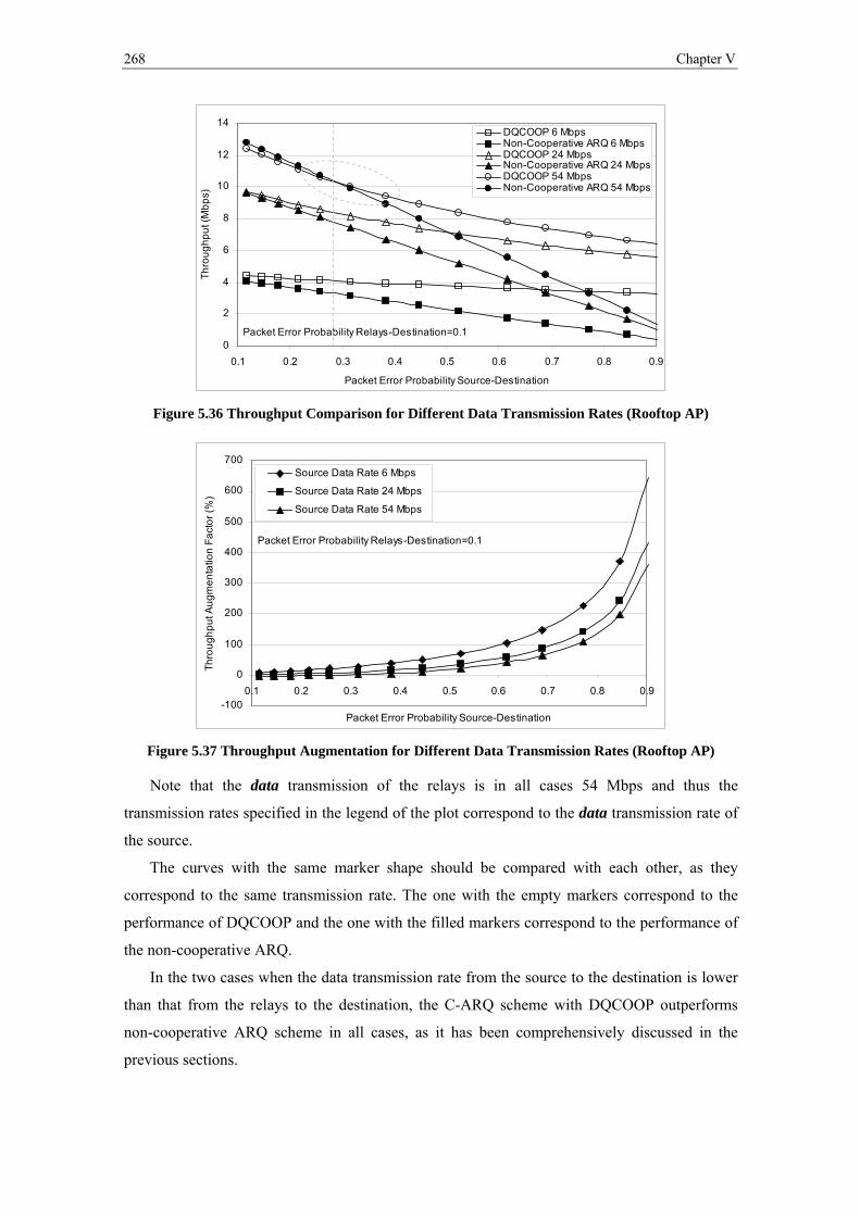
Chapter V
268
0
2
4
6
8
10
12
14
0.1 0.2 0.3 0.4 0.5 0.6 0.7 0.8 0.9
Packet Error Probability Source-Destination
Th
rou
gh
pu
t (M
bp
s)
DQCOOP 6 MbpsNon-Cooperative ARQ 6 MbpsDQCOOP 24 MbpsNon-Cooperative ARQ 24 MbpsDQCOOP 54 MbpsNon-Cooperative ARQ 54 Mbps
Packet Error Probability Relays-Destination=0.1
Figure 5.36 Throughput Comparison for Different Data Transmission Rates (Rooftop AP)
-100
0
100
200
300
400
500
600
700
0.1 0.2 0.3 0.4 0.5 0.6 0.7 0.8 0.9
Packet Error Probability Source-Destination
Th
rou
gh
pu
t Au
gm
en
tatio
n F
act
or
(%)
Source Data Rate 6 Mbps
Source Data Rate 24 Mbps
Source Data Rate 54 Mbps
Packet Error Probability Relays-Destination=0.1
Figure 5.37 Throughput Augmentation for Different Data Transmission Rates (Rooftop AP)
Note that the data transmission of the relays is in all cases 54 Mbps and thus the
transmission rates specified in the legend of the plot correspond to the data transmission rate of
the source.
The curves with the same marker shape should be compared with each other, as they
correspond to the same transmission rate. The one with the empty markers correspond to the
performance of DQCOOP and the one with the filled markers correspond to the performance of
the non-cooperative ARQ.
In the two cases when the data transmission rate from the source to the destination is lower
than that from the relays to the destination, the C-ARQ scheme with DQCOOP outperforms
non-cooperative ARQ scheme in all cases, as it has been comprehensively discussed in the
previous sections.
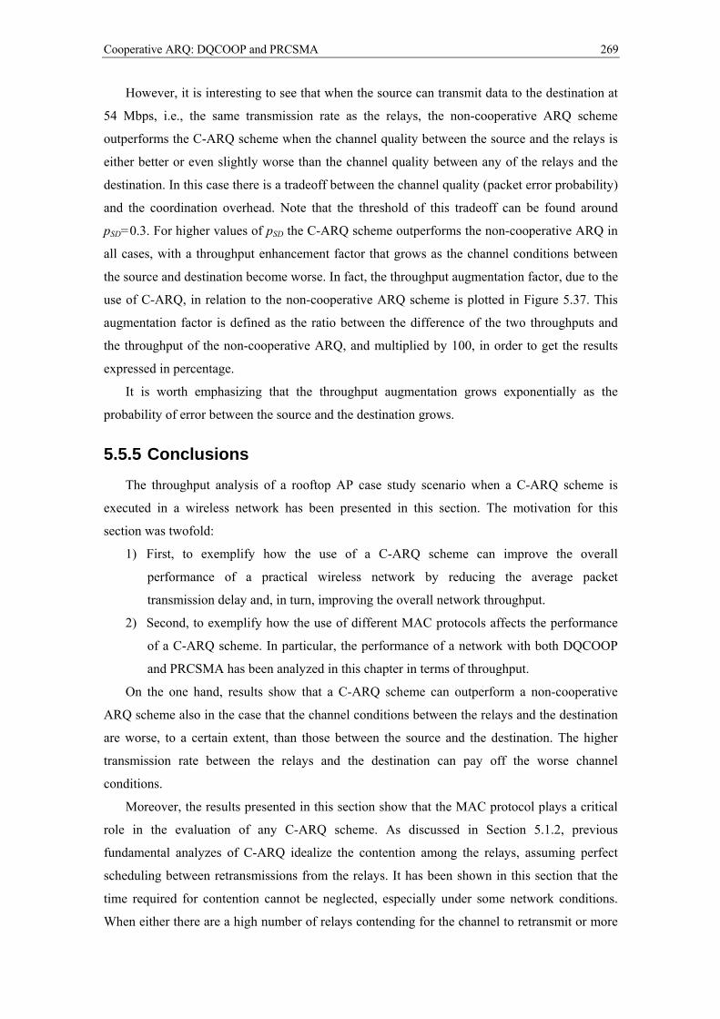
Cooperative ARQ: DQCOOP and PRCSMA 269
However, it is interesting to see that when the source can transmit data to the destination at
54 Mbps, i.e., the same transmission rate as the relays, the non-cooperative ARQ scheme
outperforms the C-ARQ scheme when the channel quality between the source and the relays is
either better or even slightly worse than the channel quality between any of the relays and the
destination. In this case there is a tradeoff between the channel quality (packet error probability)
and the coordination overhead. Note that the threshold of this tradeoff can be found around
pSD=0.3. For higher values of pSD the C-ARQ scheme outperforms the non-cooperative ARQ in
all cases, with a throughput enhancement factor that grows as the channel conditions between
the source and destination become worse. In fact, the throughput augmentation factor, due to the
use of C-ARQ, in relation to the non-cooperative ARQ scheme is plotted in Figure 5.37. This
augmentation factor is defined as the ratio between the difference of the two throughputs and
the throughput of the non-cooperative ARQ, and multiplied by 100, in order to get the results
expressed in percentage.
It is worth emphasizing that the throughput augmentation grows exponentially as the
probability of error between the source and the destination grows.
5.5.5 Conclusions
The throughput analysis of a rooftop AP case study scenario when a C-ARQ scheme is
executed in a wireless network has been presented in this section. The motivation for this
section was twofold:
1) First, to exemplify how the use of a C-ARQ scheme can improve the overall
performance of a practical wireless network by reducing the average packet
transmission delay and, in turn, improving the overall network throughput.
2) Second, to exemplify how the use of different MAC protocols affects the performance
of a C-ARQ scheme. In particular, the performance of a network with both DQCOOP
and PRCSMA has been analyzed in this chapter in terms of throughput.
On the one hand, results show that a C-ARQ scheme can outperform a non-cooperative
ARQ scheme also in the case that the channel conditions between the relays and the destination
are worse, to a certain extent, than those between the source and the destination. The higher
transmission rate between the relays and the destination can pay off the worse channel
conditions.
Moreover, the results presented in this section show that the MAC protocol plays a critical
role in the evaluation of any C-ARQ scheme. As discussed in Section 5.1.2, previous
fundamental analyzes of C-ARQ idealize the contention among the relays, assuming perfect
scheduling between retransmissions from the relays. It has been shown in this section that the
time required for contention cannot be neglected, especially under some network conditions.
When either there are a high number of relays contending for the channel to retransmit or more
Chapter V
270
than one retransmission is needed from the relays (high traffic load), the idealization of the
contention time due to the MAC problem can lead to wrong conclusions regarding the
performance of C-ARQ.
Therefore, an efficient MAC protocol is necessary to efficiently coordinate the relay
retransmissions in a C-ARQ scheme so that a performance close to the ideal perfect scheduling
can be attained. The results presented in this section have shown that, in most scenarios,
DQCOOP attains a superior performance with respect to the legacy-based PRCSMA. And what
is more important, the performance of the DQOCOP is more independent of the number of
retransmissions and the number of active relays, loosening thus the design requirements of both
the retransmission scheme and the relay selection criteria. PRCSMA, in its turn, attains good
performance in very simple scenarios with low number of required retransmissions and with a
low number of active relays. In these scenarios, even a simple ALOHA would probably do the
job.
5.6 Chapter Conclusions
This second main part of the thesis has been focused on the design and analysis of two
MAC protocols for the execution of C-ARQ schemes in wireless networks. C-ARQ schemes
have been proposed in the literature as an alternative to overcome the difficulties to deploy
MIMO systems in small mobile devices where the distance between antennas is constrained by
the size of the device itself. By allowing users to cooperate with each other, cooperative
diversity can be attained emulating a system equipped with multiple antennas. Users can
collaborate with each other to provide uncorrelated transmission paths in order to improve the
reliability or efficiency of the communications. The main idea behind C-ARQ schemes is to
exploit the broadcast nature of the wireless channel in the following manner; once a packet is
received with errors, a retransmission can be requested from any of the potential helpers which
overheard the original transmission. In this case, space diversity can be exploited. However,
involving a number of users in the communication entails a needed coordination. Previous
works in the literature (see Section 5.1.1) have shown that C-ARQ schemes can improve the
performance of wireless networks. However, these works assume simplified topologies (one
single fixed relay) and perfect scheduling among relays, when more than one is considered.
Unfortunately, this perfect scheduling is hardly possible to attain in distributed wireless
networks and thus an efficient and feasible MAC protocol is necessary. The main contributions
of this part of the thesis have been:
1) Identification of the MAC problem that comes up whenever more than one relay are
involved in a cooperation scheme.
2) Design, analysis, and performance evaluation of DQCOOP, as an innovative MAC
protocol for C-ARQ schemes.
Cooperative ARQ: DQCOOP and PRCSMA 271
3) Design, analysis, and performance evaluation of PRCSMA, as another innovative MAC
protocol for C-ARQ schemes based on the IEEE 802.11 Standard.
4) Comparison of four different ARQ schemes, considering a non-cooperative one, ideal
C-ARQ, C-ARQ with DQCOOP, and C-ARQ with PRCSMA.
5) Analysis of a case study consisting on a rooftop AP network with the execution of a C-
ARQ scheme at the MAC layer, in order to evaluate the benefits of a C-ARQ scheme
and to compare the performances of both DQCOOP and PRCSMA.
DQCOOP has been designed as a MAC protocol that can approach a perfect TDMA-
scheduling when either the number of relays or the number required retransmissions are high.
However, its overhead may reduce the enhanced performance when the number of relays is low.
In these cases, PRCSMA performs pretty well as it is a completely random access protocol.
The performances of four different ARQ schemes have been compared: a traditional non-
cooperative ARQ scheme wherein retransmissions are requested from the source, and three C-
ARQ schemes with ideal scheduling, DQCOOP, and PRCSMA.
The main conclusion of this comparison is that the overhead of the MAC protocol may
compromise the benefits of C-ARQ scheme and must be carefully considered. Previous works
in the literature idealize the problem of the contention among the relays. As it has been shown
here, this idealization can lead to wrong conclusions. It is clear that having more relays involved
in a communication can yield higher cooperative diversity gain. However, the cost of
coordinating a number of independent stations in a communication process may compromise
the benefits of C-ARQ scheme.
In the last part of this chapter, a case study consisting of the downlink of a rooftop AP and a
number of distant stations has been analyzed. Whenever a packet is received with errors at
destination, retransmissions can be requested from any of the overhearing stations as long as
they were able to decode the original packet without errors. The presented analysis and
evaluation (also supported with computer simulations) shows that the performance of this
network composition can benefit from C-ARQ schemes in almost all cases. Different channel
conditions have been considered between source and destination and between relays and
destination, showing that the C-ARQ scheme can outperform non-cooperative ARQ in most of
the channel conditions scenarios. This case study has made possible to further compare the
performances of DQCOOP and PRCSMA in a specific scenario, showing that DQCOOP
outperforms PRCSMA when the number of relays is high or when the number of required
retransmissions is bigger than one, while PRCSMA outperforms DQCOOP for simple scenarios
with a small number of relays, where indeed, any random access protocol may perform well. In
any case, the most remarkable strength of PRCSMA relies on the fact that it is strongly based on
the IEEE 802.11 Standard, facilitating thus its commercial success.
Chapter V
272
5.7 References
[1] A. Nosratinia, T. E. Hunter, and A. Hedayat, “Cooperative Communications in Wireless
Networks,” IEEE Communications Magazine, vol. 42, no. 10, pp. 74-80, Oct. 2004.
[2] The 16th WWRF Meeting, 26-28 April, 2006, Shanghai, China, http://www.wireless-
world-research.org/.
[3] M. Dianati, X. Ling, K. Naik, and X. Shen, “A Node-Cooperative ARQ Scheme for
Wireless Ad Hoc Networks,” IEEE Trans. on Vehicular Technology, vol. 55, no. 3, pp.
1032-1044, May 2006.
[4] M. Zorzi, R. R. Rao, and L.B. Milstein, “ARQ error control for fading mobile radio
channels,” IEEE Trans. on Vehicular Technology, vol. 46, no. 2, pp. 445-455, May
1997.
[5] A. Goldsmith, Wireless Communications, Cambridge University Press, 2005.
[6] S. S. Chakraborty, M. Liinaharja, and K. Ruttik, “Diversity and packet combining in
Rayleigh fading channels,” IEE Proceedings-Communications, vol. 152, no. 3, pp. 353
– 356, Jun. 2005.
[7] J. D. Morillo-Pozo and J. García-Vidal, “A Low Coordination Overhead C-ARQ
Protocol with Frame Combining,” in Proc. of the IEEE PIMRC 2007, Athens, Greece.
[8] P. Liu, Z. Tao, Z. Lin, E. Erkip, and S. Panwar, “Cooperative Wireless
Communications: A Cross-Layer Approach,” IEEE Wireless Communications
Magazine, Special Issue on Advances in Smart Antennas, pp. 84-92, Aug. 2006.
[9] IEEE, Part 11: Wireless LAN Medium Access Control (MAC) and Physical Layer
(PHY) Specifications, IEEE Std. 802.-11-99, Aug. 1999.
[10] J. Gómez and A. Pérez-Neira, “Average Rate Behavior for Cooperative Diversity in
Wireless Networks,” in Proc. of the IEEE International Symposium on Circuits and
Systems (ISCAS’06), Kos (Greece), May 21-24, 2006.
[11] S. Pfletschinger and M. Navarro, “Link Adaptation with Retransmissions for Partial
Channel State Information,” in Proc. of the IEEE GLOBECOM 2008, New Orleans,
Louisiana, USA, Nov. 2008.
[12] J. Alonso-Zárate, J. Gómez, C. Verikoukis, L. Alonso, and A. Pérez-Neira,
“Performance Evaluation of a Cooperative Scheme for Wireless Networks,” in Proc. of
the IEEE PIMRC, Helsinki, Finland, Sep. 2006.
[13] F. H. P. Fitzek and M. D. Katz, “Cooperation in Wireless Networks: Principles and
Applications,” Ed. Springer, 2006.
Cooperative ARQ: DQCOOP and PRCSMA 273
[14] E. Zimmermann, P. Herhold, and G. Fettweis, “The Impact of Cooperation on
Diversity-Exploting Protocols,” in Proc. of the 59th IEEE Vehicular Technology
Conference, 2004.
[15] E. Zimmermann, P. Herhold, and G. Fettweis, “On the Performance of Cooperative
Relaying Protocols in Wireless Networks,” European Trans. On Telecommunications,
vol. 16, no. 1, pp. 5-16, Jan. 2005.
[16] P. Gupta, I. Cerruti, and A. Fumagalli, “Three Transmission Scheduling Policies for a
Cooperative ARQ Protocol in Radio Networks,” in Proc. of the WNCG Conference,
Austin, Oct. 2004.
[17] I. Cerruti, A. Fumagalli, and P.Gupta, “Delay Model of Single-Relay Cooperative ARQ
Protocols in Slotted Radio Networks Poisson Frames Arrivals,” IEEE/ACM Trans. on
Networking, vol. 16, no. 2, Apr. 2008.
[18] J. Morillo-Pozo, J. García-Vidal, and A. I. Pérez-Neira, “Collaborative ARQ in
Wireless Energy-Constrained Networks,” in Proc. of the 2005 Joint Workshop on
Foundations of Mobile Computing 2005 (DIAL-POM’05).
[19] S. Biswas and R. Morris, "ExOR: Opportunistic Multi-hop Routing for Wireless
Networks,” in Proc. of the SIGCOMM '05, pp. 133-144, New York, NY, USA, 2005.
[20] P. Larsson and N. Johansson, "Multistation Diversity Forwarding in Multihop Packet
Radio Networks,” in Proc. of the IEEE Wireless Communications and Networking
Conference 2005, pp. 2188-2194.
[21] J. García-Vidal, M. Guerrero-Zapata, J. Morillo, and D. Fusté, “A Protocol Stack for
Cooperative Wireless Networks,” Wireless Systems and Mobility in Next Generation
Internet, in Lecture Notes in Computer Science (LNCS), vol. 4396, pp 62-73, 2007.
[22] P. Liu, Z. Tao, and S. Panwar, “CoopMAC: A Cooperative MAC for Wireless LANs,”
IEEE Journal on Selected Areas on Communications, vol. 25, no.2, Feb. 2007.
[23] T. Korakis, S. Natayanan, A. Bagri, and S. Panwar, “Implementing a Cooperative MAC
Protocol for Wireless LAN,” in Proc. of the IEEE International Conference on
Communications (ICC’06), vol. 10, pp. 4805-4810, Jun. 2006.
[24] Z. Tao, T. Korakis, Y. Slutskiy, S. Panwar, and L. Tassiulas, “Cooperation and
Directionality: A Co-opdirectional MAC for Wireless Ad Hoc Networks,” in Proc. of
the WiOpt 2007.
[25] S. Shankar, C. Chou, and M. Ghosh, “Cooperative Communication MAC (CMAC) – A
new MAC protocol for Next Generation Wireless LANs,” in Proc. of the IEEE
International Conference on Wireless Networks, Communications, and Mobile
Computing 2005.
Chapter V
274
[26] X. Wang and C. Yang, “A MAC Protocol Supporting Cooperative Diversity for
Distributed Wireless Ad Hoc Networks,” in Proc. of the IEEE PIMRC, Berlin,
Germany, Sep. 2005.
[27] A. Azgin, Y. Altunbasak, and G. AlRebig, “Cooperative MAC and Routing Protocols
for Wireless Ad Hoc Networks,” in Proc. of the IEEE GLOBECOM 2005.
[28] B. Sadek, K. J. Ray Liu, and A. Ephremides, “Collaborative Multiple-Access Protocols
for Wireless Networks,” in Proc. of the IEEE International Conference on
Communications (ICC’06), Jun. 2006.
[29] J. Gómez, J. Alonso-Zárate, C. Verikoukis, A. Pérez-Neira, and L. Alonso,
“Cooperation On Demand Protocols for Wireless Networks,” in Proc. of the IEEE
PIMRC, Athens, Greece, Sep. 2007.
[30] J. Alonso-Zárate, E. Kartsakli, A. Cateura, C. Verikoukis, and L. Alonso, “A Near-
Optimum Cross-Layered Distributed Queueing Protocol for Wireless LAN”, IEEE
Wireless Communications Magazine, Special Issue on MAC protocols for WLAN, vol.
15, no. 2, pp. 48-55, Feb. 2008.
[31] Campbell et al. “Method and apparatus for detecting collisions and controlling access to
a communications channel”, US Patent no. US6408009 B1, Jun. 2002.
[32] G. Bianchi, “Performance Analysis of the IEEE 802.11 Distributed Coordination
Function,” IEEE Journal on Selected Areas in Communications, vol. 18, no. 3, Mar.
2000.
[33] H. Wu, Y. Peng, K. Long, S. Cheng, and J. Ma, “Performance of Reliable Transport
Protocol over IEEE 802.11 Wireless LAN: Analysis and Enhancement,” in Proc. of the
INFOCOM 2002, vol. 2, pp. 559-608, Jun. 2002.
[34] J. Choi, J. Yoo, and C. Kim, “A Novel Performance Analysis Model for an IEEE
802.111 Wireless LAN,” IEEE Communications Letters, vol. 10, no. 5, May 2006.
[35] F. Alizadeh-Shabdiz and S. Subramaniam, “Analytical Models for Single-Hop and
Multi-Hop Ad Hoc Networks,” Mobile Networks and Applications 11, 75-90, 2006.
[36] P. Chatzimisios, A. C. Boucouvalas, and V. Vitsas, “IEEE 802.11 Packet Delay – A
Finite Retry Limit Analysis,” in Proc. of the IEEE GLOBECOM 2003.
[37] J. Yeo and A. Agrawala, “Packet Error Model for the IEEE 802.11 MAC Protocol,” in
Proc. of the IEEE PIMRC 2003, pp. 1722-1726, 2003.
[38] X. Zhou and J. Caffery, “Cross-layer Analysis of IEEE 802.11 DCF in Burst-Error
Fading Channels With Diversity,” in Proc. of the IEEE International Conference on
Wireless Networks, Communications and Mobile Computing, 2005, pp. 704-709, 2005.
Cooperative ARQ: DQCOOP and PRCSMA 275
[39] Z. Hadzi-Velkov and B. Spasenovski, “Saturation Throughput – Delay Analysis of
IEEE 802.11 DCF Fading Channel,” in Proc. of the ICC 2003, pp. 121-126, 2003.
[40] J. Yin, X. Wang, and P. Agrawal, “Optimal Packet Size in Error-prone Channel for
IEEE 802.11 Distributed Coordination Function,” in Proc. of the IEEE Wireless
Communications and Networking Conference ‘04, pp. 1654-1659, 2004.
[41] X. James Dong and P. Varaiya, “Saturation Throughput Analysis of IEEE 802.11
Wireless LANs for a Lossy Channel,” IEEE Comm. Letters, vol. 9, no. 2, Feb. 2005.
[42] P. Chatzimisios, A. Boucouvalas, and V. Vitsas, “Performance Analysis of IEEE
802.11 DCF in Presence of Transmission Errors,” in Proc. of the ICC,’2004, pp. 3854-
3858, 2004.
[43] IEEE Std. 802.11g, Supplement to Part 11: Wireless LAN Medium Access Control
(MAC) and Physical Layer (PHY) Specifications; Further High-Speed Physical Layer
Extension in the 2.4GHz Band.
[44] H. Bai and M. Atuiquzzaman, “Error Modeling Schemes for Fading Channels in
Wireless Communications: A Survey,” IEEE Commuinications Surveys & Tutorials,
Fourth Quarter 2003, vol. 5, no.2, pp. 2-9, 2003.
[45] H. S. Wang, “On verifying the first-order Markovian assumption for a Rayleigh fading
channel model,” IEEE Trans. on Vehicular Technology, vol. 45, no. 2, pp. 353-357,
May 1996.
[46] E. N. Gillbert, “Capacity of a Bursty-Noise Channel,” Bell System Tech. J. vol. 39, no.
9, pp. 1253-65, Sep. 1960.
[47] E. O. Elliott, “Estimates of Error Rates for Codes on Bursty-noise Channels,” Bell
System Tech, J. vol. 42, no. 9, pp. 1977-97, Sep. 1963.
[48] T. Numanoglu, B. Tavli, and W. Heinzeman, “The Effects of Channel Errors on
Coordinated and Non-Coordinated Medium Access Control Protocols,” in Proc. of the
IEEE Conference on Wireless and Mobile Computing, Networking and
Communications, vol. 1, pp. 58-65, Aug. 2005.
[49] J. R. Yee and E. J. Weldon, “Evaluation of the performance of error correcting codes on
a ilbert channel,” IEEE Trans. on Communications, vol. 43, no. 8, pp. 2316-23, Aug.
2005.
[50] J. L. Lemmon, “Wireless link statistical bit error model,” Technical Report NTIA
Report 02-394, U.S. Department of Commerce, Jun. 2002.
[51] M. Zorzi and R. R. Rao, “Lateness of probability of retransmission scheme for error
control on a two-stateMarkov channel,” IEEE Trans. on Communications, vol. 47, no.
10, pp. 1537-48, Oct. 1999.
Chapter V
276
[52] J. McDougall and S. Miller, “Sensitivity of wireless network simulations to a two-state
Markov model channel approximation,” in Proc. of the GLOBECOM 2003.
[53] A. Konrad, B. Zhao, A. Joseph, and R. Ludwig, “A Markov-based channel model
algorithm for wireless networks,” Wireless Networks, vol. 9, no. 3, pp. 189-199, May
2003.
[54] B. Gurtov and S. Floyd, “Modelling wireless links for transport protocols,” ACM
Computer Communications Review, vol. 34, no. 2, pp. 85-96, 2004.
[55] E. Modiano, “An adaptive algorithm for optimizing the packet size used in wireless
ARQ protocols,” Wireless Networks, vol. 5, no. 4, pp. 279-286, 1999.
[56] M. Zorzi, R. R. Rao, and L. B. Milstein, “ARQ Error Control for Fading Mobile Radio
Channels,” IEEE Trans. on Vehicular Technology, vol. 46, no. 2, , pp. 445-455, May
1997.
[57] D. Shiu, G. J. Foschini, M. J. Gans, and J. M. Khan, “Fading Correlation and its Effect
on the Capacity of Multi-Element Antenna Systems,” IEEE Trans. on Communications,
vol. 48, no. 3, pp. 502-513, Mar. 2000.
277
Chapter VI
6 Conclusions and Future Work
A summary of the main contributions and findings of the thesis is presented in this chapter.
The main conclusions are presented and discussed in Section 6.1, while open lines of research
are outlined in Section 6.2. Indeed, the work presented in this thesis leaves many open
challenges to be solved and this dissertation does not conclude our work in the field of MAC
protocols for wireless ad hoc networks, but it is just one main milestone in our way.
6.1 Summary and Conclusions
The thesis aims at contributing to the incessant growth of wireless communications. The
focus has been set on the design, analysis, and performance evaluation of novel MAC protocols
for wireless ad hoc networks. The thesis has been divided into one preliminary part and two
other main big parts:
1) A preliminary part comprised of Chapters I and II.
2) A first main part comprised of Chapters III and IV.
3) A second main part confined to Chapter V.
Chapter VI
278
Chapter I has been devoted to introduce the related topics, to review the state-of-the-art,
and to expose the motivations and main objectives of the thesis. Chapter II has been devoted to
define the framework of the thesis. In the second chapter, an overview of the fundamentals of
Markov chain theory and queueing theory has been presented in order to help the reader in the
understanding of the analyses developed throughout the thesis. Also in this chapter, the
MACSWIN computer simulator has been presented. All the protocols and ideas presented in
this thesis have been evaluated through a custom-made link-level simulator programmed in C++
that has been developed throughout the course of the thesis.
In Chapter III, DQMAN has been presented as a novel MAC protocol that adapts and
extends the operation of the infrastructure-based near-optimum DQCA protocol to the
distributed environment of ad hoc networks without infrastructure. A passive, spontaneous, and
dynamic master-slave clustering algorithm has been smoothly integrated with the distributed-
queueing operation of DQCA. The main idea is that any idle station that has data to transmit
seizes the channel following a CSMA-based mechanism. Once it successfully seizes the
channel, it transmits its data and it also establishes a temporary one-hop cluster wherein a
variation of the DQCA protocol is executed. Despite the cluster structure, communications may
be done by establishing peer-to-peer links between source and destination within the cluster,
i.e., there is no uplink and downlink channel separation. The cluster life time is dynamically
adjusted according to the traffic load of the network. Once an idle station gets access to the
channel and establishes a cluster, it acts as master for as long as there is data activity within the
cluster.
The performance of DQMAN for networks wherein no hidden terminals are present has
been modeled in both saturation and non-saturation conditions. By combining Markov chain
theory with classical queueing theory, an accurate model of the protocol has been developed.
This model allows for the optimization of the protocol under different metrics such as
throughput, delay, or average time in each mode of operation. The presented model, combining
spontaneous contention-based clustering and high-efficient MAC operation, constitutes one of
the main contributions of the thesis.
In addition to this model, the performance of DQMAN has been comprehensively evaluated
by means of computer simulations. Results show that, stemming from the basic definition of
DQMAN, there is room for improvement under heavy traffic conditions. Therefore, two
mechanisms have been designed to improve the performance of DQMAN in saturation
conditions.
On the other hand, the performance of DQMAN in general multi-hop networks where
hidden and exposed terminals are present has been also evaluated by means of computer
simulations. Results show that DQMAN can also run over sparsely distributed networks
Conclusions and Future Work 279
attaining good performance figures as long as some minimum, but necessary, modifications are
done the basic definition of the protocol.
A simulation-based comparison of the performances of DQMAN and the IEEE 802.11
Standard MAC protocol shows that DQMAN outperforms 802.11 in most kinds of networks in
a number of representative scenarios. The performance of the standard protocol is reasonably
good when either the number of stations or the data traffic load of the network is low. However,
its performance is severely degraded as the number of stations or the traffic load grows,
especially if the protocol parameters are not dynamically adjusted. On the contrary, DQMAN
attains a stable performance for any traffic load and its performance is almost independent of
the number of active users requesting access to the channel. DQMAN switches smoothly from a
random access control protocol to a reservation-based access protocol as the offered traffic load
of the network grows. Therefore, it attains the better of the two access methods.
Despite the high-performance of DQMAN, the IEEE 802.11 Standard has shown such a
market penetration that it is hardly realistic to believe that already deployed wireless equipment
can be drastically replaced by a new technology, no matter the higher performance it can attain.
Therefore, the last section of Chapter III has been devoted to assess the feasibility of the
compatibility and coexistence of DQMAN with legacy users. A mixed scenario composed of
both legacy 802.11 users and dual users which can execute both the rules of the standard and
DQMAN has been evaluated through computer simulation. Results show that both coexistence
and intercommunication between DQMAN and 802.11-based users is possible. The
performance of a mixed network lies in between the performance of a pure 802.11 network and
a pure DQMAN network. However, there is a tradeoff between maximum performance of the
network and fairness in the use of resources among different kinds of stations. In fact, the
maximum time a station is allowed to operate as master corresponds to the maximum duration
of a DQMAN cluster. For the duration of a cluster, legacy users cannot get access to the
channel, and thus they may suffer from channel access starvation. Therefore, it is necessary to
force DCF access periods after a DQMAN clustered operation in order to ensure access to all
the users of the network, regardless of the MAC protocol they execute. However, DCF periods
lead to lower throughput as the number of users or the traffic load grows, due to its contention-
based access. Therefore, the tradeoff between global performance and fairness has to be
efficiently managed by defining the maximum life time of DQMAN clusters.
Indeed, the rationale behind DQMAN can be applied to extend and adapt almost any other
infrastructure-based MAC protocol to operate over ad hoc networks. In order to exemplify this,
a case study has been presented in Chapter IV. DPCF has been presented as a novel MAC
protocol that adapts and extends the operation of the PCF coordination function of the IEEE
802.11 standard, designed to provide QoS in infrastructure-based networks, to ad hoc networks
without infrastructure. Link-level computer simulation with MACSWIN shows that DPCF
Chapter VI
280
outperforms DCF, validating thus the benefits obtained from the integration of spontaneous and
dynamic clustering and infrastructure-based MAC protocols together. As with DQMAN, the
coexistence and intercommunication of DPCF with legacy networks has been also evaluated
attaining very promising results.
Therefore, the main conclusion of the first main part of the thesis is that the integration of a
spontaneous, dynamic, soft-binding, and passive master-slave clustering algorithm allows
extending any high-performance infrastructure-based MAC protocol to distributed scenarios
without infrastructure, and attaining high and stable performance figures in distributed,
spontaneous, and dynamic environments.
The second main part of the thesis has turned the focus to a specific kind of cooperative
communications. The high-performance of DQMAN in networks where the users tend to get
naturally organized into clusters motivated this change of direction in the thesis. C-ARQ
schemes were identified as the perfect environment to exploit the innovative concepts of
DQMAN. Therefore, C-ARQ schemes have been introduced in Chapter V as a way of
exploiting the broadcast nature of the wireless channel to attain cooperative diversity. In short,
the idea is that in the wireless channel any transmission is not only received by the intended
destination of a message, but also by all the stations at earshot of the transmitter. What has been
typically treated as interference is used in C-ARQ schemes to provide cooperative diversity.
Whenever a destination receives a data packet with errors, it can request retransmission from
any of the stations which overheard the original transmission and can become spontaneous
relays or helpers. These helpers provide independent transmission paths and can also improve
the efficiency of the communications in terms of higher throughput, smart energy-consumption,
or even extended coverage of the communications. Several research works have analyzed the
benefits of such distributed ARQ algorithm. However, they usually idealize the required
coordination when cooperation involves a number of independent users, assuming perfect
scheduling among the relays. The fact is that when more than one spontaneous relay can assist
in one failed transmission, a Multi Relay Multiple Access (MRAC) problem arises. This MRAC
problem has been introduced in this thesis and some peculiarities that make inefficient the use
of existing MAC protocols have been identified. Accordingly, two novel MAC protocols have
been proposed to tackle with the MRAC problem of C-ARQ schemes. First, the DQCOOP has
been presented as an extension of DQMAN to efficiently operate in C-ARQ schemes.
Analogously, PRCSMA has been presented as an extension of the IEEE 802.11 Standard to
operate in C-ARQ schemes. The performances of the two protocols have been theoretically
analyzed and also evaluated through computer simulations with MACSWIN. In addition, the
performances of the two protocols have been compared to each other and also to the case when
the contention among the relays is idealized by assuming perfect scheduling among the relays
(which is the widely used approach in the literature). The main results show that DQCOOP
Conclusions and Future Work 281
outperforms PRCSMA when the number of required retransmissions or the number of active
relays (helpers) is high. On the contrary, when either the number of required retransmission or
the number of active relays is low, the random-based access of PRCSMA attains better
performance. Indeed, under these conditions, probably any random-access protocol would do
the job.
On the other hand, the most remarkable results show that idealizing the MRAC problem
may yield misleading conclusions regarding the performance of C-ARQ schemes. Indeed, the
contention among the relays cannot be idealized due to the fact that an inefficient MAC
protocol could spoil the benefits of the C-ARQ scheme. Therefore, the design of efficient MAC
protocols for C-ARQ should be further analyzed. This thesis can be considered as a first
contribution in the field.
The last section of Chapter V has been devoted to analyze a case study of the execution of a
C-ARQ scheme in a practical scenario. The performance of a representative rooftop AP network
has been evaluated taking into account the channel impairments. The performance of the
network has been evaluated with a traditional non-cooperative ARQ protocol wherein
retransmissions are only requested from the source, and with a C-ARQ scheme executing both
the DQCOOP and the PRCSMA protocols. Results demonstrate that, when the channel quality
between the source and a distant group of stations is in bad conditions, C-ARQ schemes
remarkably outperform traditional non-cooperative ARQ in terms of throughput. The results
presented in this last section of the chapter reinforce the conclusions obtained when comparing
the performances of both DQCOOP and PRCSMA.
As aforementioned, the wide range of topics covered in this thesis leaves many interesting
open challenges. The most remarkable future lines of research are outlined in the next section.
6.2 Future Work
This thesis aims at contributing to the evolution of wireless ad hoc networks not only with
the main contributions summarized in the previous section, but also by giving the floor to many
open topics that have not been covered in this thesis but they have been identified through the
course of the thesis.
Regarding the first part of the thesis, there are seven main open lines of research:
1) Once the analytical model of DQMAN has been developed and validated, a further
protocol optimization could be carried out based on this model. The maximum time a
station is allowed to operate in master mode plays a key role in the performance of the
protocol in terms of throughput. Longer cluster life times yield higher throughput, but
however, they also lead to more static cluster settings which may yield severe
unfairness in the share of the responsibility of being master. In energy-constrained
networks, long cluster life times may drain the batteries of stations operating in master
Chapter VI
282
mode. Therefore, the tradeoff between throughput and fairness constitutes an interesting
line of research.
2) The development of an analytical model for the operation of DQMAN in general multi-
hop networks constitutes one of the main lines of future research. The number of
interrelated actors in the performance of a DQMAN-based network makes its
theoretical analysis a very tough challenge.
3) Related with the previous ideas, a power consumption model of DQMAN would allow
for the assessment of the suitability of the application of DQMAN for sensor networks.
These range from large industrial sensor networks, which may be deployed over long
multi-hop paths, to intelligent ambient body sensor networks, where the sensors may
tend to be clustered and where the amount of information to transmit may be gone up.
4) The DQMAN protocol has been presented as a high-performance protocol for
infrastructureless networks. Therefore, the identification and performance evaluation of
real applications for DQMAN constitutes an important line for future research. Among
many other examples, disaster rescue operations or inter-vehicular communications can
be identified as innovative topics that are getting more relevance in the scientific
community and which match with the characteristics of DQMAN: they are
infrastructureless networks established in an ad hoc fashion to satisfy a spontaneous
need and where a high number of users, which tend to be clustered, compose a highly
loaded network.
5) The actual implementation of the protocol in real hardware is a very interesting work
ahead. Most of our efforts will be focused on developing a real testbed wherein
DQMAN can be implemented and thus the ideas presented in this thesis can be finally
validated in a real environment. The American company Ether2 (www.ether2.com) is
already implementing and commercializing DQCA for wireless centralized networks.
Our aim is to establish close collaboration with them in order to implement DQMAN in
real equipment and strive for its commercial application.
6) All the open lines for research regarding DQMAN can be extended to DPCF. In this
case, the standard-like operation of DPCF makes its implementation in real hardware
easier than in the case of DQMAN, and thus it will constitute a major part of our near
future research.
7) Finally, regarding the DPCF protocol, the study of efficient polling policies for those
stations operating in master mode constitutes an interesting topic for future research. In
addition, this is also tightly coupled with the design of efficient techniques to get some
knowledge of the local neighborhood by just overhearing ongoing transmissions.
Regarding the second part of the thesis, the analysis of the C-ARQ presented in this thesis
has been focused mainly on the design and performance of MAC protocols from the throughput
Conclusions and Future Work 283
and delay points of view. However, at least five open topics in the filed of C-ARQ have been
identified:
1) Analysis of the performance of C-ARQ schemes in terms of coverage extension and
improved energy consumption. Recall, as discussed in the introductory chapter of this
thesis, that most of the already published works are based on fundamental analyzes of
the cooperative diversity gain attained with cooperation, but, although increasing over
the last years, very few works are focused on more practical aspects of cooperation.
2) Design of efficient relay selection algorithms that select the most suitable subset of
stations to become active relays. The decision of the relay selection may be driven by
energy consumption requirements, application layer requirements, or the channel
conditions, among many other alternatives.
3) Design of efficient criteria to decide on-the-fly when cooperation should be triggered
and when an erroneous packet should be discarded for the benefit of the entire network.
4) Security issues regarding cooperation. C-ARQ schemes are built on the basis that all the
stations can overhear other transmissions to help out a failed communication. The
execution of this kind of systems may be hampered when security requirements are
introduced in the scenario. A comprehensive analysis of these issues constitutes a very
interesting line for future research.
5) As in the case of DQMAN, the implementation of both DQCOOP and PRCSMA in real
hardware constitutes one of the most interesting lines for future work. Theoretical
analysis and computer-based evaluation provide reliable performance figures with a
certain number of limitations. Therefore, the real evaluation of a C-ARQ scheme with
the two protocols would make the results more realistic and a good value for the final
assessment of the efficiency of C-ARQ schemes.
As it has been summarized in this last section, this thesis aims at contributing to the
incessant evolution of wireless networking technologies. Many contributions have been
presented, ranging from the design and modeling of innovative backwards-compatible MAC
solutions for infrastructures WLANs to efficient MAC protocols for the execution of new
cooperative communication schemes. However, it has also been identified throughout the
course of the thesis that there are still many open challenges that must be studied in order to
keep on pushing forward wireless communications, and, finally, contributing to a more
advanced wireless information society.
Related Documents