DECOHERENCE, SUPERCONDUCTING QUBITS, AND THE POSSIBILITY OF QUANTUM COMPUTING - DRAFT Jacob Portes November 2015

Welcome message from author
This document is posted to help you gain knowledge. Please leave a comment to let me know what you think about it! Share it to your friends and learn new things together.
Transcript
DECOHERENCE, SUPERCONDUCTING QUBITS, AND THE POSSIBILITYOF QUANTUM COMPUTING - DRAFT
Jacob PortesNovember 2015
I certify that I have read this dissertation and that, in my opinion, it is fully adequatein scope and quality as a dissertation for the degree of Master of Arts.
(Allan Blaer) Principal Adviser
I certify that I have read this dissertation and that, in my opinion, it is fully adequatein scope and quality as a dissertation for the degree of Master of Arts.
(Anargyros Papageorgiou) Reader
Approved for the Columbia University Graduate School of Arts and Sciences
ii
Abstract
Is it possible to implement a fully controllable, unambiguously quantum computer? While mostin the field believe that the answer is in the affirmative, uncertainty and skepticism still existamong academics and industry professionals. In particular, decoherence is often spoken of as aninsurmountable challenge. This thesis argues that there are no fundamental mathematical or physicalproperties that would preclude the possibility of implementing a fully controllable quantum computerusing superconducting qubits. The proof is in key results from the past 30 years in math, physics andcomputer science; this thesis is a sketch of these results. It begins with the well known theoreticalresults that have motivated the field - namely quantum algorithmic speed up and efficient errorcorrection - and continues with an overview of the well developed theory of decoherence, arguingthat decoherence has been and can still be significantly reduced. These theoretical results are relatedto superconducting qubits throughout. The thesis concludes with a summary of recent experimentalprogress with superconducting qubit circuits.
iii
Preface
This work is a synthesis of well established material from various subfields of quantum computing.Equations, mathematical derivations, and experimental results from published papers and booksare carefully referenced. This work was submitted in partial fulfillment of the requirements for thedegree of Master of Arts in Philosophical Foundations of Physics at Columbia University.
iv
Contents
Abstract iii
Preface iv
1 Introduction 11.1 Feynman’s Speech . . . . . . . . . . . . . . . . . . . . . . . . . . . . . . . . . . . . . 11.2 The Golden Age? . . . . . . . . . . . . . . . . . . . . . . . . . . . . . . . . . . . . . . 21.3 The Possibility of Quantum Computing . . . . . . . . . . . . . . . . . . . . . . . . . 3
1.3.1 General Skepticism . . . . . . . . . . . . . . . . . . . . . . . . . . . . . . . . . 51.3.2 Contemporary Skepticism . . . . . . . . . . . . . . . . . . . . . . . . . . . . . 6
2 Foundations of Quantum Computing 82.1 Principles of Quantum Mechanics . . . . . . . . . . . . . . . . . . . . . . . . . . . . . 8
2.1.1 The Schrodinger Equation . . . . . . . . . . . . . . . . . . . . . . . . . . . . . 92.1.2 “Coherent” Superposition . . . . . . . . . . . . . . . . . . . . . . . . . . . . . 92.1.3 Measurement and the Quantum-to-Classical Transition . . . . . . . . . . . . 102.1.4 Decoherence . . . . . . . . . . . . . . . . . . . . . . . . . . . . . . . . . . . . . 112.1.5 Spin . . . . . . . . . . . . . . . . . . . . . . . . . . . . . . . . . . . . . . . . . 122.1.6 Entanglement . . . . . . . . . . . . . . . . . . . . . . . . . . . . . . . . . . . . 13
2.2 Quantum Computing Basics: The Quantum Circuit Model . . . . . . . . . . . . . . 142.2.1 Qubit Manipulations and Gates . . . . . . . . . . . . . . . . . . . . . . . . . . 152.2.2 No Cloning Theorem . . . . . . . . . . . . . . . . . . . . . . . . . . . . . . . . 18
2.3 Early Quantum Algorithms . . . . . . . . . . . . . . . . . . . . . . . . . . . . . . . . 192.4 The Quantum Fourier Transform (QFT) . . . . . . . . . . . . . . . . . . . . . . . . . 212.5 Quantum Phase Estimation . . . . . . . . . . . . . . . . . . . . . . . . . . . . . . . . 232.6 Shor’s Algorithm . . . . . . . . . . . . . . . . . . . . . . . . . . . . . . . . . . . . . . 232.7 Grover’s Algorithm . . . . . . . . . . . . . . . . . . . . . . . . . . . . . . . . . . . . . 24
3 Quantum Error 253.1 Quantum Error Formalism . . . . . . . . . . . . . . . . . . . . . . . . . . . . . . . . . 26
3.1.1 A Simple Understanding . . . . . . . . . . . . . . . . . . . . . . . . . . . . . . 263.2 Quantum Error Correction (QEC) . . . . . . . . . . . . . . . . . . . . . . . . . . . . 27
3.2.1 Simple Error Correction: the Shor Code . . . . . . . . . . . . . . . . . . . . . 273.2.2 Stabilizer Codes . . . . . . . . . . . . . . . . . . . . . . . . . . . . . . . . . . 283.2.3 Fault Tolerance . . . . . . . . . . . . . . . . . . . . . . . . . . . . . . . . . . . 283.2.4 Threshold Theorems . . . . . . . . . . . . . . . . . . . . . . . . . . . . . . . . 283.2.5 Surface Codes . . . . . . . . . . . . . . . . . . . . . . . . . . . . . . . . . . . . 29
v
4 Superconducting Qubits 314.1 Macroscopic Quantum Behavior and Josephson Junctions . . . . . . . . . . . . . . . 324.2 Circuit Equations . . . . . . . . . . . . . . . . . . . . . . . . . . . . . . . . . . . . . . 334.3 The Charge Qubit (Cooper pair Box) . . . . . . . . . . . . . . . . . . . . . . . . . . 35
4.3.1 Tuning Junction . . . . . . . . . . . . . . . . . . . . . . . . . . . . . . . . . . 364.3.2 Manipulation . . . . . . . . . . . . . . . . . . . . . . . . . . . . . . . . . . . . 364.3.3 Qubit-Qubit Coupling and Quantum Non-Demolition (QND) Readout . . . . 37
5 The Physics of Decoherence 385.1 Density Matrices . . . . . . . . . . . . . . . . . . . . . . . . . . . . . . . . . . . . . . 385.2 Simple Model for Decoherence . . . . . . . . . . . . . . . . . . . . . . . . . . . . . . 415.3 Scattering Models . . . . . . . . . . . . . . . . . . . . . . . . . . . . . . . . . . . . . 445.4 Canonical Decoherence Models . . . . . . . . . . . . . . . . . . . . . . . . . . . . . . 445.5 Spin-Boson Model . . . . . . . . . . . . . . . . . . . . . . . . . . . . . . . . . . . . . 45
5.5.1 Set up . . . . . . . . . . . . . . . . . . . . . . . . . . . . . . . . . . . . . . . . 455.5.2 Solution . . . . . . . . . . . . . . . . . . . . . . . . . . . . . . . . . . . . . . . 465.5.3 Full Spin-Boson Model . . . . . . . . . . . . . . . . . . . . . . . . . . . . . . . 48
5.6 Spin-Bath Model . . . . . . . . . . . . . . . . . . . . . . . . . . . . . . . . . . . . . . 485.7 Decoherence in Superconducting Qubits . . . . . . . . . . . . . . . . . . . . . . . . . 49
6 Recent Progress 526.1 The Xmon Qubit (UCSB 2013) . . . . . . . . . . . . . . . . . . . . . . . . . . . . . . 526.2 5-qubit Linear Array (UCSB 2014) . . . . . . . . . . . . . . . . . . . . . . . . . . . . 536.3 9-qubit Linear Array (UCSB 2015) . . . . . . . . . . . . . . . . . . . . . . . . . . . . 546.4 4-qubit 2D Array (IBM 2015) . . . . . . . . . . . . . . . . . . . . . . . . . . . . . . . 556.5 Conclusion . . . . . . . . . . . . . . . . . . . . . . . . . . . . . . . . . . . . . . . . . 57
Bibliography 58
A Recent UCSB Publications 61
B Recent Yale Publications 63
vi
List of Figures
2.1 Bloch Sphere . . . . . . . . . . . . . . . . . . . . . . . . . . . . . . . . . . . . . . . . 132.2 Classical Computing Logic Gates (Irreversible) . . . . . . . . . . . . . . . . . . . . . 152.3 Quantum Gates . . . . . . . . . . . . . . . . . . . . . . . . . . . . . . . . . . . . . . . 172.4 The General Deutsch-Josza Algorithm . . . . . . . . . . . . . . . . . . . . . . . . . . 222.5 Quantum Fourier Transform Circuit for N = 3 . . . . . . . . . . . . . . . . . . . . . 22
3.1 Surface Code 2D Array . . . . . . . . . . . . . . . . . . . . . . . . . . . . . . . . . . 30
4.1 Cooper pair Box . . . . . . . . . . . . . . . . . . . . . . . . . . . . . . . . . . . . . . 35
5.1 “Moore’s Law” for Qubits (T2) . . . . . . . . . . . . . . . . . . . . . . . . . . . . . . 495.2 Sources of Decoherence in Superconducting Qubits . . . . . . . . . . . . . . . . . . . 506.1 Xmon Qubit . . . . . . . . . . . . . . . . . . . . . . . . . . . . . . . . . . . . . . . . . 52
6.2 5-Qubit Xmon Array . . . . . . . . . . . . . . . . . . . . . . . . . . . . . . . . . . . . 546.3 9-Qubit Linear Array . . . . . . . . . . . . . . . . . . . . . . . . . . . . . . . . . . . . 556.4 Device and circuit schematic and qubit geometry (IBM) . . . . . . . . . . . . . . . . 56
vii
Chapter 1
Introduction
The spirit of quantum computing - the motivating questions, fundamental issues, and suggestionsfor future goals - is contained in Feynman’s keynote speech and subsequent paper from the 1981Conference on Physics and Computation at MIT (Simulating Physics with computers [19]). Thefollowing is a redaction of this speech.
1.1 Feynman’s Speech
What kind of computer can be used to simulate physics? There are the approximate kinds ofsimulations, which use numerical algorithms based on simplifying assumptions in order to roughlycompute the energy of the physical system, or characterize the system dynamics. But what aboutthe exact simulation of a physical system? Is there a possibility that a computer will simulate exactlywhat nature does?
There is a worry that not all of the laws of physics can be discretized and encoded for simulation.For example, the laws of physics allow space go down to infinitesimal distances, wavelengths toincrease to infinite length, sum terms in infinite order - it would be difficult, if not impossible tosimulate these laws on a real, physical computer. However, it is not inconceivable that physicistscould discretize space and time (although we are still ways away from this).
Another worry is that the natural laws of physics are reversible, while computer logic is not.In order to simulate a reversible system exactly, wouldn’t computer logic need to be reformulatedin terms of reversible logic gates? This worry is not of much concern, as it was shown by CharlesBennett, Edward Fredkin and Tommaso Toffoli that computer logic can be formulated in terms ofreversible logic gates.1
A more serious problem is posed by quantum mechanics. Quantum mechanics involves probability- and simulating probability is computationally problematic. If a description of a physical system innature with N variables requires a general function of N variables, and if a computer simulates thisby actually computing or storing this function, then doubling the size of nature (N → 2N) wouldrequire an exponentially explosive growth in the size of the simulating computer. It is thereforeimpractical (or impossible) to simulate by calculating all the probabilities exactly.
Another approach would be to simulate the probabilities of nature with a computer which isitself probabilistic. It might not give the exact result that nature gives - but it will give results with
1Edward Fredkin and Tommaso Toffoli actually attended the conference; some of the work Feynman is referringto can be found in Toffoli’s 1980 book Reversible Computing [40]. A more recent book authored by both EdwardFredkin and Toffoli is Conservative Logic (2002) [22].
1
CHAPTER 1. INTRODUCTION 2
the same probability of nature. And by repeating the probabilistic simulation many times, it willgive the frequency of a given final state proportional to the number of times with approximately thesame rate. Is this actually possible?
The more interesting question is: why not let the computer itself be built of quantum mechanicalelements which obey quantum mechanical laws? What kind of computation could be possible withthis “quantum computer?” The implication is that a quantum computer would be able to simulatea quantum system. But the more general implication is that the capabilities of such a computerwould be far greater than any“classical” computer.
There is a worry that a computer made of quantum components might not be able to simulateall the classes of quantum problems. However, there are many phenomena in field theory that areimitated by phenomena in solid state theory - so maybe there is a set of classes of quantum mechan-ical systems that are “intersimulatable.” For example, maybe maybe finite and discrete quantummechanical systems could be simulated by a Hamiltonian involving only spin-one-half lattice an-nihilation, creation, number and identity operators locally coupled to corresponding operators onother space-time points. And finally, maybe there is even a “universal” class that can simulate everypossible quantum system - a sort of “universal quantum simulator?” Unsurprisingly, these questionsstill drive the field today.2
1.2 The Golden Age?
On September 2, 2014, Google Research Director of Engineering Hartmut Neven unceremoniouslyposted the following announcement on the Google Research Blog [2]:
The Quantum Artificial Intelligence team at Google is launching a hardware initiative todesign and build new quantum information processors based on superconducting electron-ics. We are pleased to announce that John Martinis and his team at UC Santa Barbarawill join Google in this initiative. John and his group have made great strides in build-ing superconducting quantum electronic components of very high fidelity. He recently wasawarded the London Prize recognizing him for his pioneering advances in quantum controland quantum information processing. With an integrated hardware group the QuantumAI team will now be able to implement and test new designs for quantum optimizationand inference processors based on recent theoretical insights as well as our learnings fromthe D-Wave quantum annealing architecture. We will continue to collaborate with D-Wave scientists and to experiment with the Vesuvius machine at NASA Ames which willbe upgraded to a 1000 qubit Washington processor.
The announcement was quickly picked up and shared within the academia and industry basedquantum computing communities (see the Tech Crunch and Wired articles, [1] and [3]). Thereare many research groups attempting to build quantum computers using gate model architecturewith qubit hardware ranging from photons to ion traps to NMR; Martinis’s group (along with asmattering of other research groups at Yale and elsewhere), is well known in the field for making
2He concluded the speech: “The program that Fredkin is always pushing, about trying to find a computer simulationof physics, seems to me to be an excellent program to follow out. He and I have had wonderful, intense, andinterminable arguments, and my argument is always that the real use of it would be with quantum mechanics...AndI’m not happy with all the analyses that go with just the classical theory, because nature isn’t classical, dammit, andif you want to make a simulation of nature, you’d better make it quantum mechanical, and by golly it’s a wonderfulproblem, because it doesn’t look so easy.” [19]
CHAPTER 1. INTRODUCTION 3
phenomenal progress in the past fifteen years on superconducting qubit systems. And Google isn’tthe only computer company placing its bets on superconducting qubit hardware - the IBM quantumcomputing group at IBM research has also focused recent efforts on superconducting qubits as well[13].
The fact that large tech corporations are investing in quantum computing research means thatthe field has matured significantly. Are real, physical quantum computers possible? Martinis andothers, including Google and IBM, clearly believe that the answer is yes. If so, how so?
1.3 The Possibility of Quantum Computing
Feynman essentially posed the following three questions (we will tackle the first two):
1. Is it possible to build a computer with quantum components?
2. Many problems in physics and computer science are computationally inefficient. Can quantummodels of computing tackle these problems more efficiently?
3. Would such a computer be able to simulate all quantum systems?
Without getting into too much detail, some of the important (and weird) properties of quan-tum mechanics are “coherent superposition” and “measurement ” (we’ll ignore “entanglement,” orquantum correlation, for now). If we let |0〉 represent one possible state of a quantum system, and|1〉 another possible state of a system, the “superposition” of these two states |0〉 and |1〉 is also apossible state of the quantum system:
α |0〉+ β |1〉 (1.1)
where α and β are real or imaginary numbers that satisfy the simple property |α|2 + |β|2 = 1.Quantum measurement occurs when a superposition is irreversibly “collapsed” to a single componentof superposition components:
α |0〉+ β |1〉 −→ |0〉 or |1〉 (1.2)
The probability of either outcome is given by |α|2 for |0〉 and |β|2 for |1〉. Thus if |α|2 = 1/4 and|β|2 = 3/4, then the probability of measuring |1〉 on the superposition state α |0〉+ β |1〉 is 75%. Aqubit is a quantum system that can be described by the states |0〉, |1〉 or any superposition of |0〉and |1〉 as defined by (1.1). If we treat a qubit as a single unit of information, a qubit could encodea value of |0〉, |1〉 or any superposition α |0〉 + β |1〉 of these. Often times, a qubit is described asa unit of information that can magically store both a “0 and 1 simultaneously.” While this is oneway to describe the mathematical property of “superposition,” it is important to remember thatmeasuring the qubit, however, would collapse any superposition and give a probabilistic outcome of|0〉 or |1〉.
The combination of two quantum systems, say |1〉 and |1〉, is described by the (tensor) product|1〉 ⊗ |1〉, which is often abbreviated to |1〉|1〉 or |11〉. If each of the two quantum systems is insuperposition, say the superposition (1.1), the entire two-system ensemble can be described by:
(α |0〉+ β |1〉)⊗ (α |0〉+ β |1〉) (1.3)
This could represent a two qubit ensemble. If we multiply this out, we get:
CHAPTER 1. INTRODUCTION 4
= α |0〉 ⊗ (α |0〉+ β |1〉) + β |1〉 ⊗ (α |0〉+ β |1〉) (1.4)
= α2 |0〉 |0〉+ αβ |0〉 |1〉+ βα |1〉 |0〉+ β2 |1〉 |1〉 (1.5)
The first thing to note is that two qubits in superposition can encode four possible units ofinformation - 00, 01, 10 and 11. Three qubits in superposition can encode 23 = 8 possible bits ofinformation - 000, 001, 010, 100, 011, 101, 110 and 111. It follows that N qubits can encode 2N bitsof information, which is a big deal. 500 qubits can encode 2500 bits of information (which is roughlyon the order of 10150 bits). This is enormous compared to a Terabyte -which is a measly 8 × 10¹²
bits. Given this property of quantum bits, one might expect stellar computational parallelism!Before getting too excited about this, however, it is important to remember the next rule of
quantum mechanics - Born’s rule of probabilistic outcomes. That is, when we measure a quantumcomputer, the result we get is probabilistic - and the probabilities depend on how we prepare andmanipulate the qubits. In the above equation, the outcomes are: |0〉 |0〉 with probability |α2|2, |0〉 |1〉and |1〉 |0〉 with probabilities |αβ|2 each, and |1〉 |1〉 with probability |β2|2. For α β, the mostlikely outcome of measurement is |0〉 |0〉. If α and β are equal and normalized to α, β = 1/
√2 , then
each of the four outcomes have equal measurement probability of 1/4. The outcome, of course, is a2-bit number.
The unfortunate reality is that even if we could prepare and manipulate 500 qubits (2500 bits),we would only be able to read one of those 500-qubit vectors after measurement, in the form of a500-bit number. If all the qubits were prepared in an equal superposition of 1/
√2(|0〉+ |1〉), then the
probability of measuring any one of the unique 2500 bit combinations would be 1/2500, a minisculenumber indeed. And so if we cared about the outcome of one of those, but not the rest, we wouldhave to somehow skew the probabilities of the measurement outcome such that we would get thedesired value with a sufficiently high probability (1/2500 is not particularly good - a probability of1/2 would be much better). This was and still is one of the main challenges of quantum computing.
The early goals of quantum computing were to map the language of quantum mechanics to thelanguage of computing, and then to tease out the special properties of this new kind of computing.This would take advantage of some of the unique properties of quantum mechanics such as quantumsuperposition, entanglement and coherence to perform certain algorithms more efficiently - or more“interestingly,” at the least. Deutsch’s various problems were stabs at this - they were a series of short“proof of principle” algorithms that inspired the field. Then came along two important algorithms in1994 and 1996 called Shor’s algorithm for number factorization, and Grover’s algorithm for “unsorteddatabase search.” These two algorithms have many practical applications, and have been the mainmotivation for building quantum computers [39], [25].
When Shor’s algorithm and Grover’s algorithm were first created, they did not take into ac-count the serious problems posed by quantum error. The worry was that the unique computationalspeed-up provided by these algorithms would be lost with the necessary incorporation of error cor-rection schemes. In the years that followed, a handful of quantum error correction schemes as wellas threshold theorems were proposed, and the general consensus among physicists and computerscientists alike was that provided the physical error rates of individual qubits and gates were be-low a certain threshold, Shor’s and Grover’s algorithms could be implemented with quantum errorcorrection schemes and still maintain algorithmic speed-up.
A growing group of physicists believe that it is indeed possible to physically build a quantumcomputer using superconducting Josephson junctions, or “superconducting qubits.” How wouldthis be possible? Unlike quantum algorithms, there wasn’t much progress in quantum computingexperiments until the past two decades. Superconducting qubits, for example, weren’t even seriously
CHAPTER 1. INTRODUCTION 5
considered viable qubit-like systems until the early 2000s. The idea of a superconducting qubit is tocreate a quantum system that behaved mathematically, like a 2-state quantum system. The energyground state of the system could represent |0〉 and the excited state could represent |1〉 . If it behavedquantum mechanically, it could be in a superposition as well.
In addition to having these properties, the superconducting system would have to be addressable -that is, we would have to be able to control it, initialize it, manipulate it with logic gates, and measureit - while it maintained its quantum properties of entanglement and superposition. This was in factpossible with superconducting qubits; at their core, they consist of a Josephson junction (a thinbarrier between two superconductors) that at low temperatures allows for tunneling. Interestingly,the current (or the flux) can behave like a quantum variable and form coherent superpositions. Thesuperconducting Josephson junctions could be cleverly arranged to become two level systems, andthese two level systems could in turn be tuned and controlled simply changing the current frequencyand phase.
There was a looming problem, however, and this was the issue of decoherence. In the early2000s, these superconducting qubits had very fast decoherence times - that is, they did not maintaintheir quantum behavior for more than a few nanoseconds - not much time to perform algorithms.The real success of these qubits was the dramatic increase in coherence time during the past 15years - the coherence times have increased by at least five orders of magnitude. This was in nosmall part due to a good understanding of decoherence theory as well as improvements in materialsand fabrication techniques. Today, superconducting qubits are seen as similar or even better thanthe best qubit technologies (such as trapped ions). Superconducting qubits are also fabricated likeclassical computer chips - on silicon wafer - and are thus not difficult design and manufacture.
While they claim to be close as of September 2015, Martinis’s group has not yet been able toimplement the 2D surface code - although he has succeeded in improving coherence times past thesurface code threshold [29]. Reaching these thresholds - and maintaining them as the architecturesscale - requires understanding the underlying physics in order to improve qubit coherence. But heand most of the scientists in his subfield believe that there are no fundamental limits in sight -and that quantum computers built from superconducting circuits are unambiguously within reach.The skepticism surrounding quantum computing ranges from ignorant to extremely nuanced. Thisnext section discusses some of this skepticism topically - the more rigorous discussion, of course,ensues in the subsequent chapters.
1.3.1 General Skepticism
Those with a rudimentary understanding of quantum mechanics might worry that quantum com-puters are not feasible simply because the quantum and classical worlds don’t mix. Versions of thetraditionalist Copenhagen interpretation of quantum mechanics are often taught in undergraduatephysics courses; according to these accounts, the “microscopic” world obeys quantum mechanics,and the “macroscopic” world obeys classical mechanics, and never the twain shall meet (this dualityis often referred to as Heisenberg’s cut). In addition, any sort of human manipulation or interventionis equivalent to a measurement (in the sense described above) and hence collapse. Therefore, it isnot possible to “harness” the quantum world - or so the thinking goes.
There is an easy answer to this basic skepticism - a rich, developed theory exists that doesa far better job at explaining the quantum-to-classical transition than the early interpretations ofquantum mechanics. This is the theory of decoherence developed by H. Dieter Zeh, Anthony Leggett,WojciechZureck and others in the 1970s and 1980s, that explains how quantum particles and systemscan effectively lose their quantum coherence simply by being entangled with an “environment” withmany degrees of freedom. Although they are not new fundamental axioms of quantum mechanics,the insights of decoherence have been applied to countless theoretical systems and experimental set
CHAPTER 1. INTRODUCTION 6
ups with great success. In this context, measurement can be understood as a “decoherence inducingprocess,” and manipulations can be decoherence inducing or coherence preserving, depending onhow they are implemented. We can interact with and take advantage of the quantum world in noveland exciting ways.
The real proof that we can harness the quantum world, however, is with the plethora of physicalprototypical systems of qubits, such as photons, ion traps, NMR, and of course superconductingqubits. These systems essentially are qubit systems that can be initialized, logically manipulated,entangled, and measured in most of the ways necessary to implement quantum circuits. Some ofthese technologies are further ahead than others - superconducting qubits are currently consideredone of the most viable technologies, for reasons that will become clear in Chapter 5 (for a generalcomparison of the pros and cons of the various technologies, see the review article by Ladd et al.Quantum Computers (2010) [30]).
Another basic worry, which was an entirely open question at first (but has now been quiteelegantly addressed although not completely resolved) has to do with the limitations of computing.As Feynman hinted at in his speech, how can we be sure that a quantum computer - assuming sucha contraption could be built - wouldn’t just be a souped up machine with the same fundamentallimitations as a classical computer? After all, there are a myriad of ways to implement computation;most of them, however, can be fundamentally described by the classical theory of computation.Although we might have reason to believe that a quantum computer would be different, how canthis be shown rigorously?
As mentioned above, a quantum computer could theoretically manipulate many more bits ofinformation than a classical computer - that N qubits could encode 2N bits of information, and thata single quantum timestep could operate on all superpositions/combinations simultaneously. Eventoday, this “quantum parallelism” is often touted in the media as the panacea to all computingand memory problems. The catch of course - and this was also recognized early on - was thatmeasurement that did not favor any particular outcome can render quantum parallelism useless.Early skeptics did not believe that algorithms could be designed that could overcome this problemin a way that would be as efficient or more efficient as classical computers.
While it was shown in the mid-late 1980s that any classical algorithm could be mapped onto aquantum computer, it was not until the discovery of Shor’s algorithm in 1994 and Grover’s algorithmin 1996 that it became clear that quantum computers could actually execute particular algorithmssignificantly faster than the most powerful classical computers. While some lament that there hasnot been much progress in algorithms in the past decade, there is no doubt that quantum computersare in a significant category of their own.
1.3.2 Contemporary Skepticism
A more nuanced - and legitimate - worry, is that error correction is insurmountable. What doesthis mean exactly? It is conceivable that in order to account for quantum error, elaborate errorcorrection schemes would have to be incorporated such that logical qubits were comprised of manyindividual qubits, and logical gate operations on these logical qubits were comprised of many individ-ual operations on the individual qubits. One legitimate worry is that the increased cost in numberof qubits and the timesteps of operation could be so great that it cancels any efficiency gained fromthe quantum aspect of the computation. The second, more serious worry is that necessary errorcorrection might render quantum algorithms significantly worse than classical algorithms in termsof computation efficiency. In the mid to late 1990s, a few threshold theorems were formulated thatallayed these fears, first for uncorrelated (Markovian) errors, and then for various forms of correlatederrors. While there are still a few skeptics (usually mathematicians) who argue that correlated errorsfundamentally preclude the possibility of efficient quantum computing with error correction, their
CHAPTER 1. INTRODUCTION 7
tone has softened in recent years due to the success of recent experiments.The final worry has to do with physics. We understand decoherence to a large extent, but how
can we be sure that a particular physical implementation of a qubit - whether a trapped ion or asuperconducting qubit - does not have some fundamental physical “decoherence limit.” Sure it mightbe possible to improve coherence times - but they cannot improve indefinitely. Where is the limit?And if there is a limit, then how do we know that is is above the error correction threshold?
The answer to this question is not so clear. On the one hand, a fully “error corrected” circuit(let alone computer) has not been successfully built yet. On the other hand, coherence times areimproving at a dizzying pace, with no real end in site.
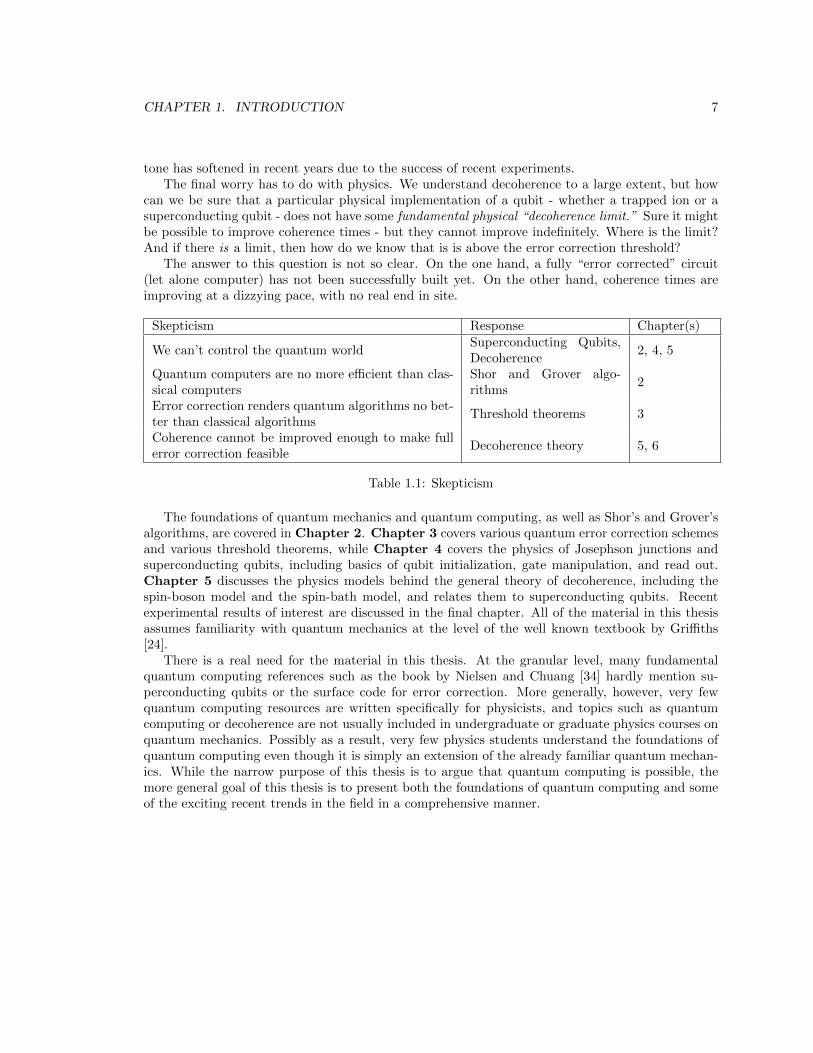
Skepticism Response Chapter(s)
We can’t control the quantum worldSuperconducting Qubits,Decoherence
2, 4, 5
Quantum computers are no more efficient than clas-sical computers
Shor and Grover algo-rithms
2
Error correction renders quantum algorithms no bet-ter than classical algorithms
Threshold theorems 3
Coherence cannot be improved enough to make fullerror correction feasible
Decoherence theory 5, 6
Table 1.1: Skepticism
The foundations of quantum mechanics and quantum computing, as well as Shor’s and Grover’salgorithms, are covered in Chapter 2. Chapter 3 covers various quantum error correction schemesand various threshold theorems, while Chapter 4 covers the physics of Josephson junctions andsuperconducting qubits, including basics of qubit initialization, gate manipulation, and read out.Chapter 5 discusses the physics models behind the general theory of decoherence, including thespin-boson model and the spin-bath model, and relates them to superconducting qubits. Recentexperimental results of interest are discussed in the final chapter. All of the material in this thesisassumes familiarity with quantum mechanics at the level of the well known textbook by Griffiths[24].
There is a real need for the material in this thesis. At the granular level, many fundamentalquantum computing references such as the book by Nielsen and Chuang [34] hardly mention su-perconducting qubits or the surface code for error correction. More generally, however, very fewquantum computing resources are written specifically for physicists, and topics such as quantumcomputing or decoherence are not usually included in undergraduate or graduate physics courses onquantum mechanics. Possibly as a result, very few physics students understand the foundations ofquantum computing even though it is simply an extension of the already familiar quantum mechan-ics. While the narrow purpose of this thesis is to argue that quantum computing is possible, themore general goal of this thesis is to present both the foundations of quantum computing and someof the exciting recent trends in the field in a comprehensive manner.
Chapter 2
Foundations of QuantumComputing
Quantum computing is built on the hallowed principles of quantum mechanics. This chapter beginswith a quick, dense review of the mathematical framework of quantum mechanics, motivated bythe important question: What exactly are the non-classical features of quantum mechanics? “Su-perposition,” “measurement” and “entanglement” are common parlance in the world of quantumcomputing, but how exactly are they defined? The next part of the chapter systematically explainshow can we use the mathematical framework of quantum mechanics for computation: how to encodeinformation in qubits, what logical manipulations are allowed, and how they fit together to formquantum circuits. Finally, the chapter concludes a brief overview of the great promises of quantumcomputing - algorithmic speed up. This includes early “proof of principle” algorithms such as thevarious Deutsch problems, as well as Shor’s algorithm and Grover’s algorithm.
2.1 Principles of Quantum Mechanics
What is it about quantum systems - and the theory of quantum mechanics - that is so unique? Let’sbegin with the basic mathematical postulates:
1. State Vector: The properties of a quantum system are completely defined by specificationof its state vector |Ψ〉. The state vector is an element of a complex Hilbert space H called thespace of states.1
2. Observables: With every physical property O (energy, position, momentum, angular mo-mentum, etc.) there exists an associated linear, Hermitian2 operator O (usually called anobservable), which acts in the space of states. The eigenvalues of the operator are the possiblevalues of the physical properties.
3. Born rule: If |ψ〉 is the vector representing the state of a system and if |φ〉 represents anotherphysical state, there exists a probability of finding |ψ〉 in state |φ〉, which is given by the squared
1Remember that the mathematical concept of a Hilbert space generalizes the notion of Euclidean space by extendingthe methods of vector algebra and calculus from the two-dimensional Euclidean plane and three-dimensional space tospaces with any finite or infinite number of dimensions. It is an abstract vector space with the structure of an innerproduct that allows length and angle to be measured
2A Hermitian matrix is a square matrix with complex entries that is equal to its own conjugate transpose. If theconjugate transpose of a matrix A is denoted by A†, then the Hermitian property can be expressed as A = A†.
8
CHAPTER 2. FOUNDATIONS OF QUANTUM COMPUTING 9
modulus of the scalar product on H: | 〈ψ|φ〉 |2. If O is an observable with eigenvalues λk andeigenvectors |k〉 such that O |k〉 = λk |k〉, the probability of obtaining λk as the outcome of themeasurement O is | 〈k|ψ〉 |2. After the measurement the state is left in the state projected onthe subspace of the eigenvalue.
4. Unitary Evolution: The evolution of a closed system is unitary.3 The state vector |ψ(t)〉 attime t is derived from the state vector |ψ(t0)〉 at time t0 by applying unitary operator U(t, t0)called the evolution operator.
How are superposition, entanglement, measurement and decoherence embedded in these postu-lates?
2.1.1 The Schrodinger Equation
The Schrodinger equation is a partial differential equation that describes how a quantum state of aphysical system changes with time
HΨ(r, t) = ihd
dtΨ(r, t) (2.1)
H is the Hamiltonian, which in most cases characterizes the total energy of the any given wavefunc-tion. If H is time independent, then the solution has the following form
Ψ(r, t) = e−iHt/hΨ(r, t), U(t) = e−iHt (2.2)
where U(t) is the evolution operator. This simple evolution operator will come up again and againboth in the context of applying gates to qubits and the various decoherence models). The familiartime independent formulation has the following structure for a single, non-relativistic particle:
EΨ = HΨ, and EΨ(r) =[− h
2µ∇2 + V (r)
]Ψ(r) (2.3)
(although this will not come up much in the context of quantum computing). While the overallform of the Schrodinger equation was not particularly surprising when it was first formulated -as it was originally motivated by the classical wave equation - it does lead to some unusual andexperimentally verified predictions such as the quantization of energy levels and the quantization ofangular momentum (position, time and momentum are not quantized, however).
2.1.2 “Coherent” Superposition
Superposition lies at the heart of quantum mechanics. Superposition is the property linear combi-nations of quantum states, represented by vectors in Hilbert space, are also quantum states. Forexample, if |ψ1〉 is a quantum state, and |ψ2〉 is a quantum state, then
|Ψ〉 =∑n
cn |ψn〉 (2.4)
is also a quantum state. Similarly, if we start off with a spin-1/2 “spin up” state |↑〉 in the |↑〉 , |↓〉basis, according to the superposition principle the state |Ξ〉 = (|↑〉+ |↓〉)/
√2 is also a quantum state.
3A matrix U is unitary if U†U = UU† = I. The importance of this to quantum logic is discussed in the followingsection.
CHAPTER 2. FOUNDATIONS OF QUANTUM COMPUTING 10
The double slit experiment is a well known experimental verification of superposition. Electronsare directed towards two slits, and produce an interference pattern on a distant screen, which isreally just a measure of spatial variation of density pattern with distribution %(x) of particles. Ifeach electron that passed through either one of the slits was simply either in the |ψ1(x)〉 state orthe |ψ2(x)〉 state, then the distribution of electron buildup on the screen over time would be
%(x) ∝ |ψ1(x)|2 + |ψ2(x)|2 (2.5)
However, the classic result is
%(x) =1
2|ψ1(x) + ψ2(x)|2 =
1
2|ψ1(x)|2 +
1
2|ψ2(x)|2 + Reψ1(x)ψ∗2(x) (2.6)
where the last term is responsible for the characteristic interference pattern on the screen. This showsthat the particles cannot be described as one and only one of the wavefunctions |ψ1(x)〉 or |ψ2(x)〉, butmust be described instead as a superposition of these wave functions |Ψ(x)〉 = (|ψ1(x)〉+|ψ2(x)〉)/
√2.
The poing its that we must be careful to emphasize a state that is a superposition of other statesdoes not simply represent a classical probabilistic ensemble of components where the system really“is” just one of the components, but we do not know which one. It is a new physical state of anindividual system and not just a statistical distribution of component states.
Unitarity is an important element of quantum mechanics - as we stated above, the operatorwhich describes the progress of a physical system in time must be a unitary operator. Why is thisso? Unitarity is essentially a restriction on the allowed evolution of quantum systems that ensuresthat the sum of all possible outcomes is 1 (the Born rule). Unitarity is defined as
U†U = UU† = I (2.7)
We can show how unitarity maintains the Born rule with the following sketch: since the prob-ability is the square of the amplitude, it can be obtained as the inner products of vectors. Theprobability amplitude of |X〉 , |Y 〉 at initial time t, is 〈X|Y 〉, and the probability amplitude of|X ′〉 , |Y ′〉 at time time t′ is 〈X ′|Y ′〉. In order for these probability amplitudes to remain the same(assuming measurement has not occurred), the time evolution operator must have the property that
U |X〉 = |X ′〉 , U |Y 〉 = |Y ′〉 −→ 〈X|Y 〉 = 〈X ′|Y ′〉 = 〈X| U†U |Y 〉 (2.8)
and hence, any evolution of a quantum system must be unitary. The importance of this for quantumcomputing cannot be understated: if we wish to implement algorithms that maintain the quantumproperties of qubits such as superposition, the operations we apply must be unitary.
2.1.3 Measurement and the Quantum-to-Classical Transition
The Measurement Problem is the problem of how or whether the wavefunction collapses during anobservation. The wavefunction evolves deterministically according to the Schrodinger equation asa linear superposition of orthogonal states, but actual measurements always find that the physicalsystem is in one of the states. It is a very strange thing, really.
How does measurement occur? One early way of understanding measurement is by postulatinga duality between quantum and classical worlds, famously known as Heisenberg’s cut. Belowthe cut everything is governed by quantum mechanics of the wave function, and above the cuteverything can be described classically. Since observation and measurement are in the classicalregime (i.e. they require macroscopic observers with macroscopic forces), any interaction with themicroscopic, quantum world would immediately induce collapse of the wavefunction . This is part of
CHAPTER 2. FOUNDATIONS OF QUANTUM COMPUTING 11
the Orthodox, or Copenhagen interpretation, and is problematic for multiple reasons (both physicaland philosophical - see Chapter 8 of Schlosshauer [37] for a more extensive discussion).
The process of measurement is better described in terms of von Neumann collapse (which isthe ancestor to decoherence theory). Von Neumann attempted to describe quantum measuremententirely in quantum terms as an interaction between a measured system and a measuring apparatus(which could be large or small, conscious or unconscious). The basic schematic is as follows. If themeasurement apparatus starts out in the “ready” state |ar〉 and the system to be measured is in the|a1〉 state, after the measurement interaction the combined system is described as
|si〉 |ar〉 → |si〉 |ai〉 (2.9)
where the measurement has established a one-to-one correspondence between the state of the systemand the state of the apparatus. In this scheme, the measurement has not altered the state of thesystem, and no entanglement has occurred thus far.
However, if the initial system-to-be-measured is in a superposition, then the linearity of theSchrodinger equation implies that the system apparatus combined will evolve according to:
|ψ〉 |ar〉 =
(∑i
ci |si〉)|ar〉 → |Ψ〉 =
∑i
ci |si〉 |ai〉 (2.10)
This of course leaves the apparatus in an entangled, superimposed state. As Schlosshauer writes, “wecan no longer attribute an individual state vector to the system or the apparatus.”4 Entanglementhas occurred, and it has occurred at the macroscopic level if the apparatus is macroscopic. Thisunitary evolution is referred to as premeasurement. So what happens next? According to vonNeumann, there are two possibilities: (1) the system can either remain entangled, or (2) collapse ofthe wavefunction can occur. This second option is referred to as strong measurement.
The measurement problem still holds, however. How does “strong measurement” actually oc-cur? In this vein, Schrodinger’s cat was a thought experiment devised by Schrodinger in 1936 inorder to highlight the weirdness of quantum mechanics at the macroscopic level - and the prob-lem of how probabilities are converted to well-defined outcomes. Various interpretative frameworkswere developed, such as Hugh Everett’s many-worlds interpretation, De Broglie-Bohm theoryof Bohmian mechanics, objective collapse models such as GRW collapse, and others to resolvethis issue. The literature on these interpretations is vast; see David Albert’s Quantum Mechanicsand Experience [5] for a simple introduction to the measurement problem, David Wallace’s bookThe Emergent Multiverse [41] for a rigorous explanation of the many-worlds interpretation, RolandOmnes’s Interpretation of Quantum Mechanics [36] and Maximillian Schlosshauer’s Decoherence andthe Quantum-to-Classical Transition [37] for rigorous explanations of the measurement problem andhow it relates to decoherence theory.
2.1.4 Decoherence
Our view of entanglement and collapse of the wave function has changed slightly since the 1930s and1940s. Quantum effects have been observed in the lab in the mesoscopic (i.e. decidedly larger thanmicroscopic) domain. In addition, it was realized that discussing and modeling quantum systemsas isolated systems was not valid in many instances. The implicit assumption that we could alwaysshield our systems from unwanted environmental disturbances was simply obscuring certain aspectsof quantum theory. In the 1970s and 1980s, new research efforts began treating quantum systemsas open systems - with a lot of success in the area of quantum optics. It was also realized that the
4The von Neumann scheme for ideal quantum measurement is described extensively in Schlosshauer pp. 50-53 [37].
CHAPTER 2. FOUNDATIONS OF QUANTUM COMPUTING 12
“isolated system” assumption had in fact been a crucial obstacle to understanding the quantum-to-classical transition. Theorists such as H. Dieter Zeh and E. Joos were able to show that the opennessof quantum systems could actually explain how quantum systems lose some of their superpositioncomponents (more on this in subsequent chapters).
It is worth mentioning in the context of decoherence and measurement that most devices capableof detecting a single particle and measuring its position strongly modify the particle’s state in themeasurement process (e.g. photons are destroyed when striking a screen). Less dramatically, themeasurement may simply perturb the particle in an unpredictable way; a second measurement, nomatter how quickly after the first, is then not guaranteed to find the particle in the same location.
However it is possible to measure a system (and collapse it if it is in a superposition) twice(or more) without changing the value of the measured system. This is a Quantum Nondemoli-tion (QND) measurement, and it is used frequently in physical qubit systems. Note that theterm“nondemolition” does not imply that the wave function fails to collapse.
2.1.5 Spin
For completeness, we state here that a “spin” S is a discrete degree of freedom that transforms likeangular momentum under rotations and corresponds to an observable describing the spin of a spin1/2 particle, in each of the three spatial directions. It is a uniquely quantum object with a finitestate space. The Pauli spin matrices are set of three 2 × 2 complex matrices that are unitary, andthey feature significantly in the quantum computing formalism.
σx =
(0 11 0
), σy =
(0 −ii 0
), σz =
(1 00 −1
)(2.11)
For a spin 1/2 particle, the spin operator is given by Si = h2 σi. A spin Hamiltonian (almost
always) consists of a sum of one-spin and two-spin terms. This is very analogous to the Hamiltonianof a particle system, where one has one-body terms (an external potential) plus two-body terms(particle-particle interactions). For example, a general spin Hamiltonian can be be composed of amagnetic field coupling HB = −HB
∑giµBSi where HB is the magnetic field, and an exchange
interaction (sometimes called Heisenberg Exchange Hamiltonian) Hex = −∑i,j JijSi · Sj . In a
crystal, generalization of the Heisenberg Hamiltonian in which the sum is taken over the exchangeHamiltonians for all the (i, j) pairs of atoms of the many-electron system gives:
HHeis =1
2
−2J∑i,j
Si · Sj
= −∑i,j
JSi · Sj (2.12)
We will see a similar Hamiltonian used for spin-bath coupling decoherence models in Chapters 5 and6. Unsurprisingly, two level quantum systems can be described using the spin operator formalism.Since information is traditionally encoded in 0s and 1s, it makes sense to describe the quantum bitas a binary system as well i.e. a two dimensional complex Hilbert space with orthonormal bases|0〉 , |1〉.
For completeness, we mention here that the Bloch sphere is a useful visualization of pure stateof a two level quantum system.
|Ψ〉 = eiγ(
cos(θ
2) |0〉+ eiφ sin(
θ
2) |1〉
)(2.13)
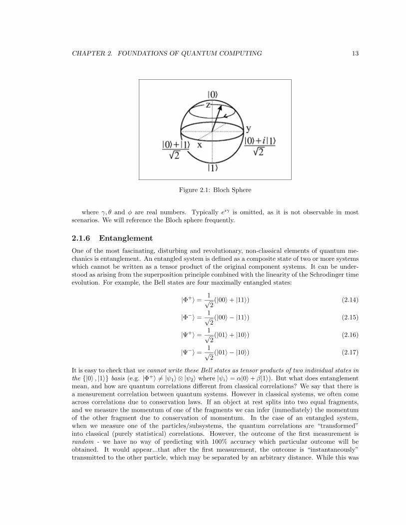
CHAPTER 2. FOUNDATIONS OF QUANTUM COMPUTING 13
Figure 2.1: Bloch Sphere
where γ, θ and φ are real numbers. Typically eiγ is omitted, as it is not observable in mostscenarios. We will reference the Bloch sphere frequently.
2.1.6 Entanglement
One of the most fascinating, disturbing and revolutionary, non-classical elements of quantum me-chanics is entanglement. An entangled system is defined as a composite state of two or more systemswhich cannot be written as a tensor product of the original component systems. It can be under-stood as arising from the superposition principle combined with the linearity of the Schrodinger timeevolution. For example, the Bell states are four maximally entangled states:
|Φ+〉 =1√2
(|00〉+ |11〉) (2.14)
|Φ−〉 =1√2
(|00〉 − |11〉) (2.15)
|Ψ+〉 =1√2
(|01〉+ |10〉) (2.16)
|Ψ−〉 =1√2
(|01〉 − |10〉) (2.17)
It is easy to check that we cannot write these Bell states as tensor products of two individual states inthe |0〉 , |1〉 basis (e.g. |Φ+〉 6= |ψ1〉 ⊗ |ψ2〉 where |ψi〉 = α|0〉+ β|1〉). But what does entanglementmean, and how are quantum correlations different from classical correlations? We say that there isa measurement correlation between quantum systems. However in classical systems, we often comeacross correlations due to conservation laws. If an object at rest splits into two equal fragments,and we measure the momentum of one of the fragments we can infer (immediately) the momentumof the other fragment due to conservation of momentum. In the case of an entangled system,when we measure one of the particles/subsystems, the quantum correlations are “transformed”into classical (purely statistical) correlations. However, the outcome of the first measurement israndom - we have no way of predicting with 100% accuracy which particular outcome will beobtained. It would appear...that after the first measurement, the outcome is “instantaneously”transmitted to the other particle, which may be separated by an arbitrary distance. While this was
CHAPTER 2. FOUNDATIONS OF QUANTUM COMPUTING 14
originally considered a troubling aspect of the theory of quantum mechanics (see the famous 1935“EPR” paper Can quantum mechanical description of physical reality be considered complete? byEinstein, Podolsky and Rosen [18]), entanglement is now considered an indisputable part of quantummechanics. John Bell’s book Speakable and Unspeakable in Quantum Mechanics [9] contains a moreextensive discussion on entanglement and the role it plays in our current understanding of quantummechanics.
The maximally entangled Greenberger-Horne-Zeilinger (GHZ) state is simply an extension of theBell |Ψ+〉 state for N > 2 qubits:
|GHZ〉 =|0〉⊗N + |1〉⊗N√
2(2.18)
where |0〉⊗N is the N -tensor product. For example, the simplest entangled state N = 3 is:
|GHZ〉 =|000〉+ |111〉√
2
As we shall see later, many experiments (e.g. [8] and [29]) create and maintain GHZ states asa measure of how well their hardwares can entangle their qubits. This is particularly importantbecause by various measures of entanglement (there is no standard measure), the GHZ is consideredmaximally entangled.5 If one of the qubits is measured (as either 0 or 1), however, the states are nolonger entangled. In contrast, the W state is defined as:
|W 〉 =1√N
(|100..0〉+ |010...0〉+ ...+ |00...01〉) (2.19)
and has multiparticle entanglement such that when one qubit is measured, the remaining qubits arestill entangled.
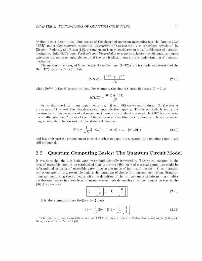
2.2 Quantum Computing Basics: The Quantum Circuit Model
It was once thought that logic gates were fundamentally irreversible. Theoretical research in thearea of reversible computing established that the irreversible logic of classical computers could bereformulated in terms of reversible gates (one-to-one maps of input and output). Since quantumevolutions are unitary, reversible logic is the paradigm of choice for quantum computing. Standardquantum computing theory begins with the definition of the primary units of information - qubits- orthogonal states in a two level quantum system. We define these two component vectors in the|0〉 , |1〉 basis as
|0〉 =
[10
], |1〉 =
[01
](2.20)
It is also common to use the|+〉 , |−〉 basis
|+〉 =1√2
(|0〉+ |1〉) =1√2
[11
](2.21)
5Interestingly, it wasn’t explicitly studied until 1989 by Daniel Greenberg, Michael Horne and Aaron Zeilinger inGoing Beyond Bell’s Theorem [23].
CHAPTER 2. FOUNDATIONS OF QUANTUM COMPUTING 15
Figure 2.2: Classical Computing Logic Gates (Irreversible)
|−〉 =1√2
(|0〉 − |1〉) =1√2
[1−1
](2.22)
We define the tensor product of two qubits as:
|0〉 ⊗ |0〉 = |00〉 =
[10
]⊗[
10
]=
1×[
10
]0×
[10
] =
1000
|01〉 =
0100
, |10〉 =
0010
, |11〉 =
0001
The tensor product of 3 qubits gives vectors of length 23 = 8, and so on (we can see that the
Dirac bra-ket notation makes dealing with the tensor product of many qubits less cumbersome thanvector notation).
2.2.1 Qubit Manipulations and Gates
The natural choice of unitary transformations to use for two level quantum systems are:
X =
[0 11 0
], Y =
[0 −ii 0
], Z =
[1 00 −1
](2.23)
which are the same matrices as the Pauli σ matrices mentioned above. Interpreted in the contextof logic operations, the Pauli-X is simply a NOT gate
X |0〉 =
[0 11 0
] [10
]→[
01
]= |1〉 , X |1〉 → |0〉
CHAPTER 2. FOUNDATIONS OF QUANTUM COMPUTING 16
as it flips the state |0〉 to |1〉 and the state |1〉 to |0〉. The Z-gate has no classical analogy, as itrotates |1〉 to −|1〉 but does nothing to |0〉:
Z |1〉 =
[1 00 −1
] [01
]→ −
[01
]= − |1〉
Gates can also be applied one after another.6
While the above gates are the most obvious operators to introduce into the quantum circuitmodel, there are three more important single qubit gates that play a role in the quantum algorithmsto come. These gates are the Hadamard gate H, the phase gate S, and the shift gate T (also calledthe π/8-gate).
H =1√2
[1 11 −1
](2.24)
S =
[1 00 i
](2.25)
T = eiπ/8[e−iπ/8 0
0 eiπ/8
]=
[1 00 eiπ/4
](2.26)
The Hadamard gate has the important property of putting the |0〉 and |1〉 states in superpositions.This is equivalent to switching from the |0〉 , |1〉 basis to the |+〉 , |−〉 basis:
H |0〉 =1√2
[1 11 −1
] [10
]=
1√2
[11
]=
1√2
(|0〉+ |1〉) = |+〉 , H |1〉 = |−〉
H |−〉 =1√2
[1 11 −1
]1√2
[1−1
]=
1
2
[02
]= |1〉 , H |+〉 = |0〉
Pauli spin matrices exponentiated7 give rise to three useful classes of unitary matrices called rotation
6These matrices are operators, and order matters. Conventionally, the rightmost operator is applied first, suchthat:
XZ |0〉 =
[0 11 0
] [1 00 −1
] [10
]=
[0 11 0
] [10
]= |1〉
ZX |0〉 =
[1 00 −1
] [0 11 0
] [10
]=
[1 00 −1
] [01
]= − |1〉
Both of these are distinct from X⊗ Z |0〉 ⊗ |1〉 = X |0〉Z |1〉, where X⊗ Z is a 2-qubit operator, or a 4× 4 matrix.7Note that the function of an operator can be expressed as f(A) =
∑i f(λi) |ai〉 〈ai|, where λi is an eigenvalue
and |ai〉 is an eigenvector. Since the eigenvectors of Z are |0〉 and |1〉 with eigenvalues 1 and −1, we can write
e−iθZ/2 = e−iθ(1)/2 |0〉 〈0|+ e−iθ(−1)/2 |1〉 〈1| =[e−iθ/2 0
0 eiθ/2
]
CHAPTER 2. FOUNDATIONS OF QUANTUM COMPUTING 17
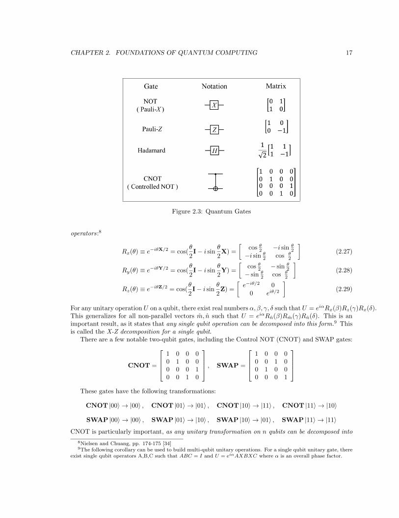
Figure 2.3: Quantum Gates
operators:8
Rx(θ) ≡ e−iθX/2 = cos(θ
2I− i sin
θ
2X) =
[cos θ2 −i sin θ
2
−i sin θ2 cos θ
2
](2.27)
Ry(θ) ≡ e−iθY/2 = cos(θ
2I− i sin
θ
2Y) =
[cos θ2 − sin θ
2
− sin θ2 cos θ
2
](2.28)
Rz(θ) ≡ e−iθZ/2 = cos(θ
2I− i sin
θ
2Z) =
[e−iθ/2 0
0 eiθ/2
](2.29)
For any unitary operation U on a qubit, there exist real numbers α, β, γ, δ such that U = eiαRx(β)Rz(γ)Rx(δ).This generalizes for all non-parallel vectors m, n such that U = eiαRn(β)Rm(γ)Rn(δ). This is animportant result, as it states that any single qubit operation can be decomposed into this form.9 Thisis called the X-Z decomposition for a single qubit.
There are a few notable two-qubit gates, including the Control NOT (CNOT) and SWAP gates:
CNOT =
1 0 0 00 1 0 00 0 0 10 0 1 0
, SWAP =
1 0 0 00 0 1 00 1 0 00 0 0 1
These gates have the following transformations:
CNOT |00〉 → |00〉 , CNOT |01〉 → |01〉 , CNOT |10〉 → |11〉 , CNOT |11〉 → |10〉
SWAP |00〉 → |00〉 , SWAP |01〉 → |10〉 , SWAP |10〉 → |01〉 , SWAP |11〉 → |11〉
CNOT is particularly important, as any unitary transformation on n qubits can be decomposed into
8Nielsen and Chuang, pp. 174-175 [34]9The following corollary can be used to build multi-qubit unitary operations. For a single qubit unitary gate, there
exist single qubit operators A,B,C such that ABC = I and U = eiαAXBXC where α is an overall phase factor.
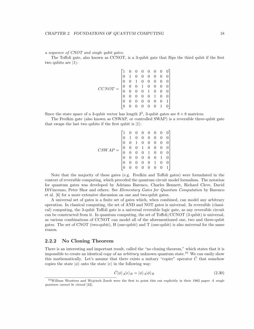
CHAPTER 2. FOUNDATIONS OF QUANTUM COMPUTING 18
a sequence of CNOT and single qubit gates.The Toffoli gate, also known as CCNOT, is a 3-qubit gate that flips the third qubit if the first
two qubits are |1〉:
CCNOT =
1 0 0 0 0 0 0 00 1 0 0 0 0 0 00 0 1 0 0 0 0 00 0 0 1 0 0 0 00 0 0 0 1 0 0 00 0 0 0 0 1 0 00 0 0 0 0 0 0 10 0 0 0 0 0 1 0
Since the state space of a 3-qubit vector has length 23, 3-qubit gates are 8× 8 matrices.
The Fredkin gate (also known as CSWAP, or controlled SWAP) is a reversible three-qubit gatethat swaps the last two qubits if the first qubit is |1〉:
CSWAP =
1 0 0 0 0 0 0 00 1 0 0 0 0 0 00 0 1 0 0 0 0 00 0 0 1 0 0 0 00 0 0 0 1 0 0 00 0 0 0 0 0 1 00 0 0 0 0 1 0 00 0 0 0 0 0 0 1
Note that the majority of these gates (e.g. Fredkin and Toffoli gates) were formulated in the
context of reversible computing, which preceded the quantum circuit model formalism. The notationfor quantum gates was developed by Adriano Barenco, Charles Bennett, Richard Cleve, DavidDiVincenzo, Peter Shor and others. See Elementary Gates for Quantum Computation by Barencoet al. [6] for a more extensive discussion on one and two-qubit gates.
A universal set of gates is a finite set of gates which, when combined, can model any arbitraryoperation. In classical computing, the set of AND and NOT gates is universal. In reversible (classi-cal) computing, the 3-qubit Toffoli gate is a universal reversible logic gate, as any reversible circuitcan be constructed from it. In quantum computing, the set of Toffoli/CCNOT (3 qubit) is universal,as various combinations of CCNOT can model all of the aforementioned one, two and three-qubitgates. The set of CNOT (two-qubit), H (one-qubit) and T (one-qubit) is also universal for the samereason.
2.2.2 No Cloning Theorem
There is an interesting and important result, called the “no cloning theorem,” which states that it isimpossible to create an identical copy of an arbitrary unknown quantum state.10 We can easily showthis mathematically. Let’s assume that there exists a unitary “copier” operator C that somehowcopies the state |φ〉 onto the state |e〉 in the following way:
C|φ〉A|e〉B = |φ〉A|φ〉B (2.30)
10William Wootters and Wojciech Zurek were the first to point this out explicitly in their 1982 paper A singlequantum cannot be cloned [42].
CHAPTER 2. FOUNDATIONS OF QUANTUM COMPUTING 19
for all possible states |φ〉 in the state space. It must be unitary if it is a non-measurement, timeevolution on the state. This seems fine; however, if we select an arbitrary pair of states |φ〉A and|ψ〉A and try to copy them we run into trouble. Because C is unitary, it preserves the inner product,so the inner product after the copier is applied must remain the same:
〈e|B〈φ|A|ψ〉A|e〉B = 〈e|B〈φ|AC†C|ψ〉A|e〉B = 〈φ|B〈φ|A|ψ〉A|ψ〉B , (2.31)
Equating the left hand side and right hand sides
〈φ|ψ〉A〈e|e〉B = 〈φ|ψ〉A = 〈φ|ψ〉2AB
This implies that either 〈φ|ψ〉 = 1 or 〈φ|ψ〉 = 0, so we obtain either φ = ψ or φ and ψ are
orthogonal. However, this cannot be the case for two arbitrary states (e.g. φ = 12 |0〉 +
√3
2 |1〉 and
φ = 1√2|0〉 + 1√
2|1〉 whose inner product is equal to 1+
√3
2√
2) . Therefore a single universal gate C
cannot clone a general quantum state. However, a copier could clone equal or orthogonal states.The implications of the no cloning theorem for quantum algorithms and quantum error correction
are important. Let’s say we manipulate some qubits as part of a routine (i.e. as part of a generalquantum algorithm or as part of a an error correction protocol), and want to duplicate the resultsof this routine without measurement in order to proceed to the next part of the algorithm. The nocloning theorem states that this is simply not possible.
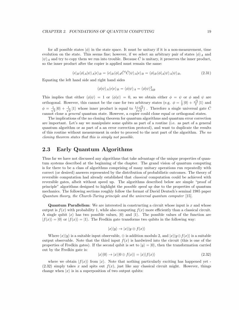
2.3 Early Quantum Algorithms
Thus far we have not discussed any algorithms that take advantage of the unique properties of quan-tum systems described at the beginning of the chapter. The grand vision of quantum computingis for there to be a class of algorithms comprising of many unitary operations run repeatedly withcorrect (or desired) answers represented by the distribution of probabilistic outcomes. The theory ofreversible computation had already established that classical computation could be achieved withreversible gates, albeit without speed up. The algorithms described below are simple “proof ofprinciple” algorithms designed to highlight the possible speed up due to the properties of quantummechanics. The following sections roughly follow the format of David Deutsch’s seminal 1985 paperQuantum theory, the Church-Turing principle and the universal quantum computer [15].
Quantum Parallelism: We are interested in constructing a circuit whose input is x and whoseoutput is f(x) with probability 1, while also computing f(x) more efficiently than a classical circuit.A single qubit |x〉 has two possible values, |0〉 and |1〉. The possible values of the function are|f(x)〉 = |0〉 or |f(x)〉 = |1〉. The Fredkin gate transforms two qubits in the following way:
|x〉|y〉 → |x〉|y ⊕ f(x)〉
Where |x〉|y〉 is a suitable input observable, ⊕ is addition modulo 2, and |x〉|y⊕f(x)〉 is a suitableoutput observable. Note that the third input f(x) is hardwired into the circuit (this is one of theproperties of Fredkin gates). If the second qubit is set to |y〉 = |0〉, then the transformation carriedout by the Fredkin gate is:
|x〉|0〉 → |x〉|0⊕ f(x)〉 = |x〉|f(x)〉 (2.32)
where we obtain |f(x)〉 from |x〉. Note that nothing particularly exciting has happened yet -(2.32) simply takes x and spits out f(x), just like any classical circuit might. However, thingschange when |x〉 is in a superposition of two output qubits:
CHAPTER 2. FOUNDATIONS OF QUANTUM COMPUTING 20
|x〉 =1√2
(|0〉+ |1〉) −→ f
(1√2
(|0〉+ |1〉))
=1√2
(|f(0)〉+ |f(1)〉)
Already we can see that the Fredkin gate will process information about both |f(0)〉 and |f(1)〉.Mathematically this turns into:
|x〉|0〉 → |x〉|f(x)〉 (2.33)
1√2
(|0〉+ |1〉
)|0〉 → 1
2
(|0〉+ |1〉
)(|f(0)〉+ |f(1)〉
)(2.34)
=1
2
(|0〉|f(0)〉+ |1〉|f(0)〉+ |0〉|f(1)〉+ |1〉|f(1)〉
)(2.35)
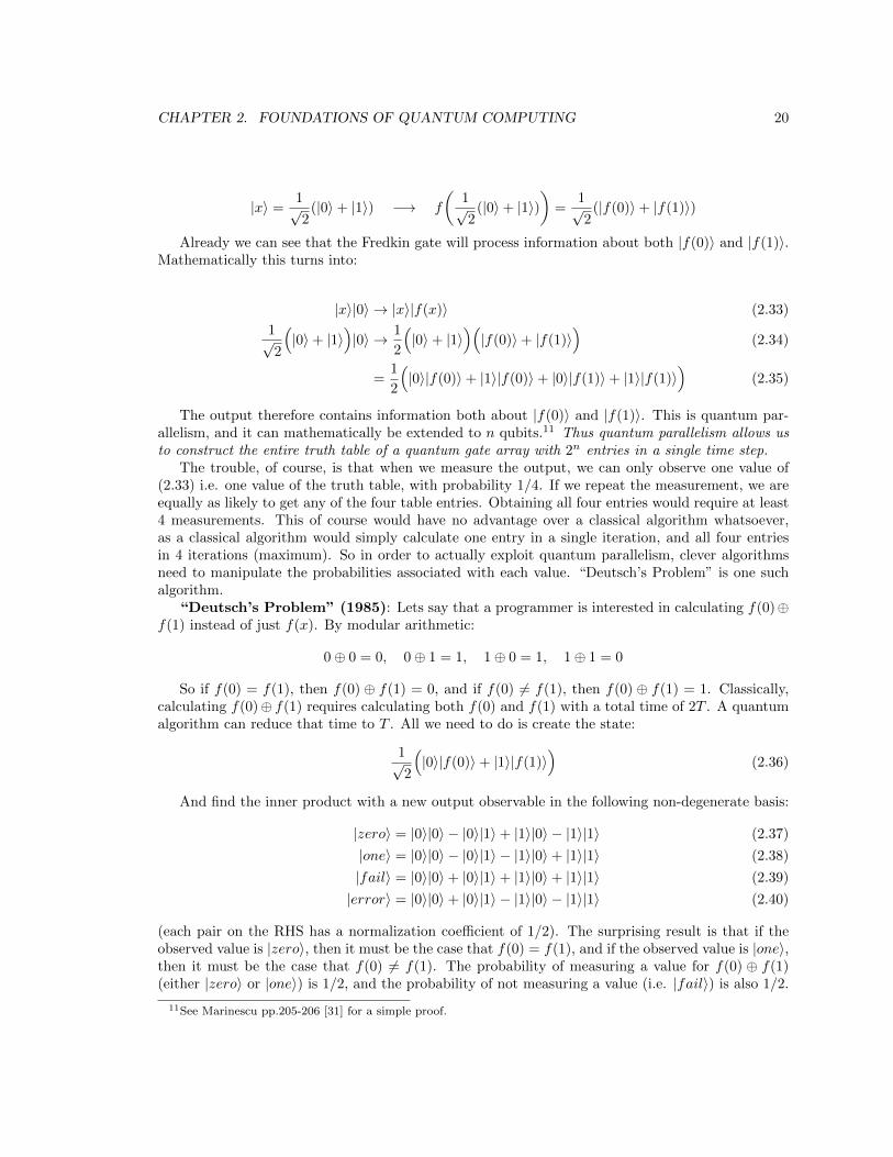
The output therefore contains information both about |f(0)〉 and |f(1)〉. This is quantum par-allelism, and it can mathematically be extended to n qubits.11 Thus quantum parallelism allows usto construct the entire truth table of a quantum gate array with 2n entries in a single time step.
The trouble, of course, is that when we measure the output, we can only observe one value of(2.33) i.e. one value of the truth table, with probability 1/4. If we repeat the measurement, we areequally as likely to get any of the four table entries. Obtaining all four entries would require at least4 measurements. This of course would have no advantage over a classical algorithm whatsoever,as a classical algorithm would simply calculate one entry in a single iteration, and all four entriesin 4 iterations (maximum). So in order to actually exploit quantum parallelism, clever algorithmsneed to manipulate the probabilities associated with each value. “Deutsch’s Problem” is one suchalgorithm.
“Deutsch’s Problem” (1985): Lets say that a programmer is interested in calculating f(0)⊕f(1) instead of just f(x). By modular arithmetic:
0⊕ 0 = 0, 0⊕ 1 = 1, 1⊕ 0 = 1, 1⊕ 1 = 0
So if f(0) = f(1), then f(0) ⊕ f(1) = 0, and if f(0) 6= f(1), then f(0) ⊕ f(1) = 1. Classically,calculating f(0)⊕ f(1) requires calculating both f(0) and f(1) with a total time of 2T . A quantumalgorithm can reduce that time to T . All we need to do is create the state:
1√2
(|0〉|f(0)〉+ |1〉|f(1)〉
)(2.36)
And find the inner product with a new output observable in the following non-degenerate basis:
|zero〉 = |0〉|0〉 − |0〉|1〉+ |1〉|0〉 − |1〉|1〉 (2.37)
|one〉 = |0〉|0〉 − |0〉|1〉 − |1〉|0〉+ |1〉|1〉 (2.38)
|fail〉 = |0〉|0〉+ |0〉|1〉+ |1〉|0〉+ |1〉|1〉 (2.39)
|error〉 = |0〉|0〉+ |0〉|1〉 − |1〉|0〉 − |1〉|1〉 (2.40)
(each pair on the RHS has a normalization coefficient of 1/2). The surprising result is that if theobserved value is |zero〉, then it must be the case that f(0) = f(1), and if the observed value is |one〉,then it must be the case that f(0) 6= f(1). The probability of measuring a value for f(0) ⊕ f(1)(either |zero〉 or |one〉) is 1/2, and the probability of not measuring a value (i.e. |fail〉) is also 1/2.
11See Marinescu pp.205-206 [31] for a simple proof.
CHAPTER 2. FOUNDATIONS OF QUANTUM COMPUTING 21
Thus the quantum algorithm computes f(0)⊕ f(1) in a single step with a probabilistic success rateof 1/2.
In 1992, David Deutsch and Richard Jozsa improved this idea with a deterministic algorithm(generalized to a function which takes n bits input). Unlike Deutsch’s Problem, this algorithmrequired two function evaluations instead of only one. Further improvements to the Deutsch-Jozsaalgorithm were made by Richard Cleve and others in Quantum algorithms revisited [12] resulting inthe Deutsch-Josza Algorithm that is both deterministic and requires only a single query of f(x). TheDeutsch-Jozsa algorithm provided inspiration for Shor’s algorithm and Grover’s algorithm, whichwe shall cover later in this chapter. The next algorithm below is is a special case of the generalDeutsch-Josza algorithm.
“Deutsch’s Algorithm” (1998): Similar to above, we want to check whether a function iseither balanced or constant; i.e. if f(0) = f(1) or f(0) 6= f(1). If f(0) ⊕ f(1) = 0, then functionsare balanced, and if f(0) ⊕ f(1) = 1, then the functions are constant. We are given a quantumimplementation of the function f(x) that maps |x〉 |y〉 to |x〉 |f(x)⊕ y〉. First apply the Hadamardgate to each qubit
HH |0〉 |1〉 = H |0〉H |1〉 −→ 1
2(|0〉+ |1〉)(|0〉 − |1〉) (2.41)
=1
2|0〉 (|0〉 − |1〉) +
1
2|1〉 (|0〉 − |1〉) (2.42)
apply function f(x) via the unitary gate Uf(x)
=1
2|0〉 (|f(0)⊕ 0〉 − |f(0)⊕ 1〉) +
1
2|1〉 (|f(1)⊕ 0〉 − |f(1)⊕ 1〉) (2.43)
=1
2(−1)f(0) |0〉 (|0〉 − |1〉) +
1
2(−1)f(1) |1〉 (|0〉 − |1〉) (2.44)
= (−1)f(0) 1
2
(|0〉+ (−1)f(0)⊕f(1) |1〉
)(|0〉 − |1〉
)(2.45)
(this requires some algebra). We ignore the global phase, and apply the Hadamard gate to eachqubit:
= (−1)f(0)H1√2
(|0〉+ (−1)f(0)⊕f(1) |1〉
)H
1√2
(|0〉 − |1〉
)(2.46)
=1
2
(|0〉+ (−1)f(0)⊕f(1) |0〉
)|1〉+
1
2
(|1〉 − (−1)f(0)⊕f(1) |1〉
)|1〉 (2.47)
=1
2
(1 + (−1)f(0)⊕f(1)
)|0〉 |1〉+
1
2
(1− (−1)f(0)⊕f(1)
)|1〉 |1〉 (2.48)
When the first qubit is measured, if the function is balanced the outcome will be |0〉 with probability1, and if the function is constant the outcome will be |1〉 with probability 1. This deterministicallyreturns an answer in a single algorithmic iteration. While this algorithm doesn’t have many prac-tical purposes, it undoubtedly proves the possibility of algorithmic speedup with quantum computers.
2.4 The Quantum Fourier Transform (QFT)
The Quantum Fourier Transform (QFT) is the quantum analogue of the discrete fourier transform,and is an important part of many quantum algorithms including Shor’s algorithm. The QFT gate
CHAPTER 2. FOUNDATIONS OF QUANTUM COMPUTING 22
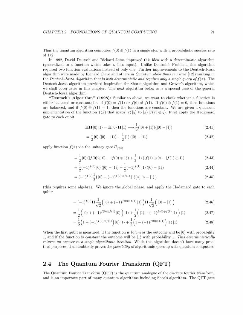
Figure 2.4: The general Deutsch-Josza algorithm begins with the n + 1 bit state |0〉⊗n|1〉 and
examines the probability of measuring |0〉⊗n, | 12n
∑2n−1x=0 (−1)f(x)|2 which evaluates to 1 if f(x) is
constant and 0 if f(x) is balanced.
acts on quantum state∑N−1i=0 xi |i〉 and maps it to a quantum state
∑N−1i=0 yi |i〉 according to the
formula
yk =1√N
N−1∑j=0
xje2πijk/N (2.49)
where ω is often substituted for e2πi/N . This is possible because the fourier transform is unitary andcan be expressed as a unitary matrix FN
FN =
1 1 1 1 . . . 11 ω ω2 ω3 . . . ωN−1
1 ω2 ω4 ω6 . . . ω2(N−1)
1 ω3 ω6 ω9 . . . ω3(N−1)
......
......
...1 ωN−1 ω2(N−1) ω3(N−1) . . . ω(N−1)(N−1)
For example, for N = 4, w = i and
F4 =1
2
1 1 1 11 i −1 −i1 −1 1 −11 −i −1 i
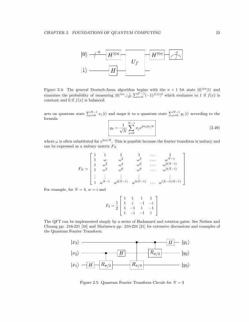
The QFT can be implemented simply by a series of Hadamard and rotation gates. See Nielsen andChuang pp. 216-221 [34] and Marinescu pp. 210-224 [31] for extensive discussions and examples ofthe Quantum Fourier Transform.
Figure 2.5: Quantum Fourier Transform Circuit for N = 3
CHAPTER 2. FOUNDATIONS OF QUANTUM COMPUTING 23
2.5 Quantum Phase Estimation
The quantum phase estimation algorithm is a quantum algorithm that finds many applicationsas a subroutine in other algorithms. The algorithm allows us to estimate the eigenphase θ ofan eigenvector |ψ〉 of a unitary gate U (where U |ψ〉 = eiθ |ψ〉), given access to a quantum stateproportional to the eigenvector and a procedure to implement the unitary gate conditionally. Notethat the Quantum Fourier Transform is part of the phase estimation algorithm. See Nielsen andChuang pp. 221-247 [34] for a rigorous treatment of quantum phase estimation and its role in Shor’salgorithm.
2.6 Shor’s Algorithm
Shor’s algorithm is quantum algorithm for integer factorization, formulated in 1994 by Peter Shor[39]. The problem posed is: given a composite integer N , find a factor (any nontrivial factor willdo). It is substantially faster than the fastest known classical number factorization algorithm, calledthe general number field sieve (although it is possible that an unknown faster classical algorithmmight exist).12 Much of the excitement surrounding Shor’s algorithm has to do with the possibilitythat it could be used to break public-key encryption schemes such as RSA, which is based on theassumption that factoring large numbers is computationally intractable.
Shor’s algorithm consists of two parts: (1) reducing the factoring problem to the problem of order-finding (2) solving the order finding problem with a quantum algorithm, which can be thought ofas the quantum phase estimation algorithm in disguise. Scott Aaronson explains the algorithm wellwithout much mathematical formalism; the following sketch is based off his explanation [4]. A morerigorous explanation of Shor’s algorithm and the derivation of its computational complexity can befound in Nielsen and Chuang pp. 226-247 [34] and Marinescu pp. 224-247 [31].
As we hinted at previously, an efficient quantum algorithm needs to exploit some structure ofthe problem in order to “skew” the measurement outcome such that the outcome is probabilisticallycorrect. The integer factorization problem does have some structure - in fact, it can be reduced toperiod finding. What exactly is period finding, then?
We start off by noticing that we can express the powers of 2 as powers of 2 mod 15:
2, 4, 8, 16, 32, 64, 128, 256, 512, 1024, . . . −→ 2, 4, 8, 1, 2, 4, 8, 1, 2, 4, . . .
It is clear from this that the powers of 2 mod 15 are periodic. The powers of 2 mod 21 are also periodic:2, 4, 8, 16, 32, 64, 128, 256, 512, 1024, . . . −→ 2, 4, 8, 16, 11, 1, 2, 4, 8, 16, etc. The generalization of thisby Euler states that if N is product of two prime number p and q, then the sequence:
x mod N, x2 mod N, x3 mod N, x4 mod N, . . . (2.50)
will repeat with some period that evenly divides (p−1)(q−1), provided x is not divisible by p or q. Itfollows that if N = 15, then the prime factors of N are p = 3 and q = 5, so (p− 1)(q − 1) = 8. Andthe period of 2 mod 15 is 4, which evenly divides 8. Similarly, for N = 21, then p = 3 and q = 7, so(p−1)(q−1) = 12. And the period of 2 mod 21 is 6, which evenly divides 12. This means that, if wecan find the period of a sequence that van be expressed in the form of (2.50), then we can uncovera “hidden” structure of the prime factors of N (namely, a divisor of (p− 1)(q− 1)). And in order tofind the period, we simply need to apply the (quantum) Fourier transform over the superposition of
12Specifically, the cost of Shor’s algorithm is O((logN)3) using fast multiplication, which is polynomial in thenumber of bits needed to represent N , or “polylogN .” It is substantially faster than the general number field sieve,
which works in “sub-exponential time” about O(e1.9(logN)1/3(log logN)2/3 ) [39]
CHAPTER 2. FOUNDATIONS OF QUANTUM COMPUTING 24
xmod N, x2mod N, x3mod N etc. (luckily it is possible to generate this superposition). The reasonthis is not efficient on a classical computer is that the period of the sequence might be extremelylarge, i.e. it could have N might have hundreds or thousands of digits, and it is therefore impracticalto store or manipulate on a classical computer. This of course is not an issue for a quantum computerwith an N -qubit register that encodes 2N bits of information. So if we apply the Quantum FourierTransform to this particular superposition of states, the outcome will be a new superposition of stateswhich is probabilistically weighted towards the vector/state representing the period. This is repeated,and the outcomes are used to reconstruct the original prime factors.
Until now the Quantum Fourier Transform was simply a unitary operation - a tool and notan algorithm. When included in Shor’s algorithm, however, it is the key to quantum algorithmicefficiency. This is because the outcome of the QFT depends on the input i.e. the superposition ofstates. So when a problem can be reduced to a question of finding the period, the Quantum FourierTransform can be used to skew the measurement statitistics.
2.7 Grover’s Algorithm
Grover’s algorithm finds unique input to a black box function that produces a particular outputvalue using just O(N1/2) evaluations of the function, where N is the size of the function’s domain.This only produces quadratic speed up as opposed to the exponential speed up of Shor’s algorithm.While it was originally described as a database search algorithm, it is better described as an invertingfunction, i.e. for a function y = f(ω), calculate ω given y.
f is the function which maps database entries to 0 or 1 where f(ω) = 1 if and only if ω satisfiesthe search criterion. The algorithm relies on the existence of “quantum black box” access to asubroutine Uω which is a unitary operator with the following properties:
Uω |ω〉 = − |ω〉Uω |x〉 = |x〉 for all x 6= ω
Assuming such a subroutine exists and is efficient, the goal is to identify index |ω〉.The algorithm is simply:
1. Initialize the system to a superposition over all states
|s〉 =1√N
N−1∑x=0
|x〉
2. Perform the Grover iteration r(N) times: this is defined as applying operator Uω, then applyingthe Grover diffusion operator Us = 2 |s〉 〈s| − I.
3. Measure: the result will be eigenvalue λω with probability approaching 1 for N 1. Fromλω, ω may be obtained
Note that if we are dealing with a database, it is not represented explicitly but rather by index-reading a full database item by item could take a much longer time than Grover’s search algorithm.Nielsen and Chuang pp. 248 - 261 [34] and Marinescu pp. 246-261 [31] discuss Grover’s algorithmin more detail.
Chapter 3
Quantum Error
“The marvel of the present result [re the threshold theorem] is that it proves that, tothe best of our current knowledge, no principle in physics will limit quantum computersfrom being realized someday” Nielsen and Chuang, p.494
It was understood early on that quantum systems are inherently noisy. How difficult it wouldbe to manage this quantum noise was studied in the mid-90s by Landauer, Unruh, and others. Theworry, of course, was that implementing error correction on quantum circuits would render any“quantum algorithmic efficiency” (such as that achieved by Shor’s algorithm) useless. It would beeven worse if quantum error correction required such an overhead of resources that it made quantumcomputers significantly worse than classical computers.
Luckily, these fears never materialized, and in the ensuing years various efficient error correctionschemes were designed (such as Shor’s code, CSS, the surface code and others) that cleverly tackledthe issue of error correction. Of particular importance were the various threshold theorems, whichshowed that a quantum computer could simulate an ideal quantum computer, provided the levelof noise is below a certain threshold. These threshold theorems imply that the error in quantumcomputers can be controlled as the number of qubits scales up. They also imply that algorithmslike Shor’s algorithm and Grover’s algorithm would still be more efficient than classical algorithmseven with error correction. Of all the error correction schemes, the surface code takes advantageof particular properties of qubits such as parity to reduce the threshold necessary to implementefficient computation (this is why it is favored among suqperconducting qubit research groups).The stabilizer code, for example, has a threshold around pth ≈ 10−4 while the surface code has athreshold around pth ≈ 10−2. Depending how much better coherence is than the minimum thresholdfor a particular implementation, it is estimated that error correction will account for the majorityof quantum information processing (which is not the most exciting prospect).
The main sources for this section are Nielson and Chuang [34], Schlosshauer [37] and Martinis’sextensive surface code paper [21]. Unfortunately this chapter is somewhat topical and covers justenough material to understand error correction in the context of quantum computing. Where thenoise comes from, and how exactly it affects these systems, is discussed in subsequent chapters.
25
CHAPTER 3. QUANTUM ERROR 26
3.1 Quantum Error Formalism
3.1.1 A Simple Understanding
How do we model noise in a classical system? Let’s start with a simple example of bit 0 that hasprobability p of flipping to 1 through some noisy process, and similarly for bit 1→ 0. If X is initialstate of the bit, and Y is the final state of the bit, probability dictates:
p(Y = y) =∑x
p(Y = y|X = x)p(X = x)
where conditional probabilities p(Y = y|X = x) are called transition probabilities. Rewriting inmatrix form with p0, p1 as initial probabilities that the bits are in the states 0 and 1, and q0, q1 ascorresponding probabilities after noise has occurred[
q0
q1
]=
[1− p pp 1− p
] [p0
p1
]where the center matrix is evolution matrix E. This assumes that consecutive noise processesare independent, is physically reasonable in many situations. More generally, it treats results asstochastic Markov processes. Although quantum errors are quite different from classical errors, wecan generalize this probabilistic paradigm to the class of quantum errors by simply assuming thatat every time step of a quantum manipulation, there is an associated probability of error p.
There are five general kinds of quantum errors:
amplitude damping - If a qubit is in excited state |1〉, amplitude damping causes qubit to“relax” to the ground state |0〉 by losing energy to the environment (for example, in the form of aphoton when a single atom coupled to a single mode of electromagnetic radiation undergoes spon-taneous emission). However, if a qubit is in the ground state, no change occurs.
phase damping - Phase damping (also called the phase flip) is a noise process that describesa change in phase of the quantum state. For example, a 1√
2(|0〉 + |1〉) state might transform to a
1√2(|0〉 − |1〉) state. Phase damping is uniquely quantum mechanical, and can even describe loss of
quantum information without loss of energy. As Nielsen and Chuang write that “phase damping isone of the most subtle and important processes in the study of quantum computation and quantuminformation.”1 As an aside, T2 is often referred to as the “Transverse coherence time” or “phasedamping time” and it essentially describes how long the phase term of the qubit can be controlled.This will be discussed further in the discussion of decoherence.
bit flip - This noise simply flips the qubit from |0〉 to |1〉 (and vice versa).
bit-phase flip - The bit-phase flip is a combination of the bit flip and the phase flip (notingthat Y = iXZ). Thus, 1√
2(|0〉+ |1〉) −→ − 1√
2(|1〉+ |1〉) is an example of a bit-phase flip.
depolarizing channel - This is a channel where the amplitude of the state uniformly contracts,regardless of value or phase.
1Nielsen and Chuang, p. 385 [34]

CHAPTER 3. QUANTUM ERROR 27
3.2 Quantum Error Correction (QEC)
3.2.1 Simple Error Correction: the Shor Code
In order to protect against the effects of these possible errors, we can encode information by includingredundant information. One simple example is to replace a single qubit with three qubits |0〉 →|000〉 = |0L〉 , |1〉 → |111〉 = |1L〉 which we call a logical qubit. Suppose initial state a |0〉+ b |1〉 waslogically encoded such that |0L〉 + b |1L〉 = a |000〉 + b |111〉 , and that a bit flip occurred on one ofthe qubits. A simple error correction procedure to recover the original state would be:
1. Error Detection (syndrome diagnosis): perform an operation that indicates which qubitflipped, if any. There are four projection operators:
P0 ≡ |000〉 〈000|+ |111〉 〈111| no error
P1 ≡ |100〉 〈100|+ |011〉 〈011| bit flip qubit 1
P2 ≡ |010〉 〈010|+ |101〉 〈101| bit flip qubit 2
P3 ≡ |001〉 〈001|+ |110〉 〈110| bit flip qubit 3
Note that the syndrome only contains information about which error has occured, but noinformation about the value of a or b (i.e. no information about the state being protected).
2. Recovery Use value of error syndrome to decide which procedure to use to recover initialstate. If P0 do nothing, if P1 then flip first qubit, etc.
This correction scheme works well provided bit flips occur on no more than one of the three qubits.This occurs with probability (1− p)3 + 3(1− p)2 = 1− 3p2 + 2p3 and the probability of the error notbeing corrected is therefore 3p2−2p3. If p < 1/2, then the probability of the error being corrected is> 1/2. However, if the probability of error is > 1/2, then the probability of the error being correctedis < 1/2.
This only applies to bit flip errors - however as we saw above, there are other kinds of errors.Interestingly, there is a simple way to convert the phase flip channel into a bit flip channel. Thephase flip operator Z is applied to state a |0〉+ b |1〉 such that it becomes a |0〉 − b |1〉. In |+〉 , |−〉basis the Z operator acts as a bit flip: Z |+〉 = |−〉. Hence for phase-flip correction, we can simplyencode logical qubits as |0L〉 = |+ + +〉 , |1L〉 = |− − −〉. All operations needed for error correctionare performed in a similar manner to the bit flip channel but in the |+〉 , |1〉 by including theHadamard transform H where necessary. The Shor code is a simple quantum code which can protectagainst the effects of arbitrary error on single qubit. It takes advantage of the three qubit bit flipand phase flip codes. First encode using the phase flip code |0〉 → |+ + +〉 , |1〉 → |− −−〉 and thenencode each of the three qubits using the bit flip code, such that each |+〉 → 1
2√
2(|000〉+ |111〉) and
|−〉 → 12√
2(|000〉 − |111〉) . The result is a nine qubit code:
|0〉 → |0L〉 ≡1
2√
2
(|000〉+ |111〉
)(|000〉+ |111〉
)(|000〉+ |111〉
)|1〉 → |1L〉 ≡
1
2√
2
(|000〉 − |111〉
)(|000〉 − |111〉
)(|000〉 − |111〉
)The Shor code was one of the first error correction schemes.
CHAPTER 3. QUANTUM ERROR 28
3.2.2 Stabilizer Codes
Stabilizer codes (or additive quantum codes) are an important class - many states can be moreeasily described by working with the operators that stabilize them than by working explicitly withthe state itself. And many error correction schemes (including Shor’s code and CSS) can be morecompactly described using stabilizer formalism than state vector formalism. Stabilizer formalismalso allows for systematic construction procedures for encoding, decoding and error-correction.
3.2.3 Fault Tolerance
The basic idea of fault-tolerance is to compute directly on encoded states without decoding them. Ifwe assume noise can affect every element of computation (state preparation, quantum gates, mea-surement procedure, transmission of quantum information along wires, etc.), we must replace eachqubit in the original circuit with an encoded block of qubits and replace each gate with a procedurefor performing encoded gate acting on the encoded state. Applying error correction periodically isnot sufficient to prevent the build up of errors
1. Encoded gates can cause errors to propagate. Therefore encoded gates must be designedcarefully such that failure during procedure can only propagate to a small number of qubitsin each block (called fault tolerant procedures).
2. Error correction itself can introduce errors on encoded qubits, so this must be accounted foras well
The fault tolerance of a procedure is defined as the property that if only one component o the pro-cedure fails, then the failure causes at most one error in each encoded block of qubits output fromthe procedure.2
3.2.4 Threshold Theorems
There is a remarkable result - the threshold theorem - that arbitrarily good quantum computationcan be achieved even with faulty logic gates provided only that error probability per gate is belowa constant threshold. The result is based on concatenated codes which can be used to reduce theeffective error rate achieved by computation even further. We can recursively apply a particularscheme for simulating a circuit using an encoded circuit by constructing a hierarchy of circuits. Iffailure of physical qubit is p, then failure at one level of encoding is cp2, at two levels of encoding is
c(cp2)2. Concatenating k times, probability of failure at highest level is (cp)2k
/c, while the size ofthe simulating circuit goes as dk times the size of the original circuit (d is a constant representingmaximum number of operations used in fault tolerant procedure to do encoded gate and error-correction).
One of the earlier threshold theorems stated the following:Threshold Theorem A quantum circuit containing p(n) gates may be simulated with probabilityof error at most ε using
O(poly(log p(n)/ε)p(n))
gates on hardware whose components fail with probability at most p provided p is below someconstant threshold p < pth and given reasonable assumptions about the noise in the underlyinghardware.
2Nielsen Chuang p. 476 [34]
CHAPTER 3. QUANTUM ERROR 29
For the Steane code, pth ≈ 10−4. The most important result of error correction codes is theresult that provided noise in individual quantum gates is below a certain constant threshold, it ispossible to efficiently perform an arbitrarily large quantum computation . The conclusion, then, isthat quantum error does not pose an existential threat for quantum computation.
It is important to note the assumptions made for the early threshold theorems. It is certainlyreasonable that physical implementations of qubits might experience more varied forms of noise thatdon’t fit into the above formulation, such as
1. Correlated error in time (i.e. the noise is non-Markovian)
2. Correlated error due to spatial considerations
Finally, it is important to realize that threshold result requires parallelism, and doesn’t take intoaccount classical communication elements, inclusion of ancilla qubit generation etc. However, manymore sophisticated models have been developed since the first threshold theorems, and the generalidea of a threshold still holds for these as well.
3.2.5 Surface Codes
Surface codes are a particular class of code that take advantage of symmetrical properties of groupsof qubits (such as parity) to correct quantum errors. They were somewhat obscure until recently,and are not mentioned in Nielsen and Chuang. Some consider it an even more robust type of errorcorrection that only needs nearest neighbor correlation and has lower threshold values than thetraditional codes mentioned above. Surface codes: Towards practical large-scale quantum computa-tion by Fowler, Mariantoni, Martinis and Cleland 2012 [21] is a fantastic resource with a wealth ofinformation about surface codes. Below is one figure from this paper.
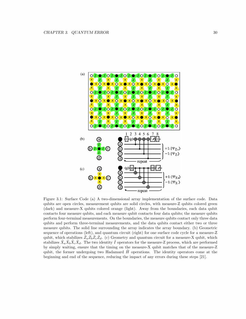
CHAPTER 3. QUANTUM ERROR 30
Figure 3.1: Surface Code (a) A two-dimensional array implementation of the surface code. Dataqubits are open circles, measurement qubits are solid circles, with measure-Z qubits colored green(dark) and measure-X qubits colored orange (light). Away from the boundaries, each data qubitcontacts four measure qubits, and each measure qubit contacts four data qubits; the measure qubitsperform four-terminal measurements. On the boundaries, the measure qubits contact only three dataqubits and perform three-terminal measurements, and the data qubits contact either two or threemeasure qubits. The solid line surrounding the array indicates the array boundary. (b) Geometricsequence of operations (left), and quantum circuit (right) for one surface code cycle for a measure-Zqubit, which stabilizes ZaZbZcZd. (c) Geometry and quantum circuit for a measure-X qubit, whichstabilizes XaXbXcXd. The two identity I operators for the measure-Z process, which are performedby simply waiting, ensure that the timing on the measure-X qubit matches that of the measure-Zqubit, the former undergoing two Hadamard H operations. The identity operators come at thebeginning and end of the sequence, reducing the impact of any errors during these steps [21].
Chapter 4
Superconducting Qubits
While we have reviewed much of the theoretical foundation of quantum computing, from the circuitmodel to quantum error correction, the question still remains: how is it possible to physically imple-ment a qubit -and for that matter, a quantum computer? While there are many possible physicalimplementations of qubits, including photons, ion traps and NMR, superconducting qubits are cur-rently considered one of the most successful and feasible technologies. This has to due with the factthat, over the past decade, the quantum coherence of superconducting qubits has increased morethan five orders of magnitude (more on this in subsequent chapters).
Superconducting qubits are essentially variations of Josephson junction circuits with inductors,capacitors and resonators in addition to Josephson junctions. The circuits are very similar to dissi-pationless LC circuits (i.e. simple harmonic oscillators) at extremely low temperatures, except thatthe Josephson junctions behave like nonlinear inductive elements and affect the oscillator potentialsuch that it becomes anharmonic. The anharmonicity, of course, is key as it means that the differentenergy levels may be addressed at different frequencies. When tuned appropriately, higher energylevels can be ignored and the circuit becomes a two level system (with a ground state and an excitedstate) which is a robust representation of a qubit.
The qubit can be controlled by applying a sinusoidal driving force (similar to a classical circuit).The frequency of the driving wave causes rotations about the z-axis, and the phase of the drivingvoltage causes rotations about the x and y axis. This allows for complete control of the state ofthe qubit. Finally, measurement can be done by reading the signal from a resonator coupled to thequbit.
In this way, with superconducting qubits we have:
1. Representation of quantum information
2. Application of unitary transforms
3. Preparation of a fiducial input state
4. Measurement of output
The majority of the material in this chapter was referenced from Superconducting Quantum Bits(2008) by Clarke and Wilhelm [11], Steven Girvin’s chapter on circuit QED from Quantum Ma-chines: Measurement and Control of Engineered Quantum Systems: Lecture Notes of Les HouchesSummer School (chapter 3) [16], Superconducting Qubits: A Short Review by Devoret, Wallraff andMartinis [17], as well as great course notes by Andreas Wallraff, and Theo Walter from the ETH
31
CHAPTER 4. SUPERCONDUCTING QUBITS 32
Zurich QSIT 2015 course.1 All of these resources discuss the physics of superconducting circuits ex-tensively. Unfortunately the standard reference for quantum computing, Nielson and Chuang [34],only mentions superconducting qubits in a single paragraph.
4.1 Macroscopic Quantum Behavior and Josephson Junc-tions
There are two important definitions related to Josephson junctions:
1. flux quantization, whereby magnetic flux in superconducting ring is quantized
Φ0 = h/2e ≈ 2.07× 10⁻¹⁵Tm (4.1)
2. Josephson Tunneling, where cooper pairs can tunnel through energy barrier coherently.Supercurrent I through the barrier is related to the gauge invariant phase difference δ(t)between the phases of the two superconductors:
I = I0sin(δ(t)) (4.2)
where I0 is the critical current, a phenomenological property of the junction. The phase
difference changes in time as hdδ(t)dt = hω = 2eV , where ω is the angular frequency at whichthe supercurrent oscillates.
We introduce the operators δ and N associated with the Josephson coupling energy Ej =I0Φ0/2π and the charging energy Ec = (2e)2/2C.
When Josephson junctions were fist investigated in the 1960s, it was found that macroscopicquantum tunneling occured and that energy levels were quantized [28]. Cooper pairs tunnel from|0〉 state through barrier when I < I0 and then run freely down the washboard potential, generatinga voltage of 2∆s/e, which can be detected easily. Energy quantization was found by irradiatingjunction with microwaves, since each energy level has a unique frequency due to the anharmonicnature of the potential.
In the 1980s, Anthony Leggett predicted that it would be possible to demonstrate a superpositionof macroscopic flux states in Josephson junction devices. This was not achieved experimentally until1997 and 2000 by Nakamura with a charge qubit and Friedman and Caspar Van der Waal with fluxqubits.
The next step is to show that the nonlinear inductance alters the Hamiltonian of the LC circuitin order to solve for the new energy levels of the system. There are many different ways of doing this- either with a coax line, capacitor or inductor coupled with voltage. The so called “phase qubit”is with coax line and forms a natural phase basis, the “charge qubit” is with a capacitor and formsa charge basis, and the “flux qubit” is with an inductor and forms a flux basis. The Cooper pairbox, or charge qubit is currently the most used configuration, and is the basis of the quantronium,transmon and then xmon qubits. We will therefore focus on the charge qubit.
1These notes can be accessed at qudev.ethz.ch/node/114091 and qudev.ethz.ch/content/QSIT15/QSIT15 Super L02 slides.pdf
CHAPTER 4. SUPERCONDUCTING QUBITS 33
4.2 Circuit Equations
The following is a rough and simple derivation of the quantum analogue to the LC Circuit. Theclassical circuit equations are:
Φ = LI VL = −LdIdt
Q = CVC (4.3)
Emag =1
2LI2 Eelec
1
2CV 2 (4.4)
where Φ magnetic flux of the inductor, L is inductance, I is the current, Q is the total chargeon capacitor C is the capacitance, VL is the voltage across inductor, VC is the voltage across thecapacitor, and E is the energy stored in inductor capacitor respectively. Ignoring resistance, thebasic circuit Hamiltonian is:
HLC =1
2CV 2 +
1
2LI2 =
1
2
Q2
C+
1
2
Φ2
L(4.5)
If we treat Q as p and Φ as x, recalling that:
δH
δp= x
δH
δx= −p, δH
δΦ=
Φ
L= I = Q
δH
δQ=Q
C= V = −LI = −Φ (4.6)
Making the jump from classical to quantum by treating x and p as operators x and p, we havethe quantum Hamiltonian:
Hq =1
2
Q2
C+
1
2
Φ2
L=
1
2
h
C
δ2
δΦ2+
1
2
1
LΦ2 (4.7)
Which has all the expected properties of a quantum harmonic oscillator such as energy En =
hω(n+ 1
2
).
This can be expressed in second quantization form:
H = hω(a†LC aLC +1
2) (4.8)
aLC =1√
2hZC
(ZCQ+ iΦ
)a†LC =
1√2hZC
(ZCQ− iΦ
)(4.9)
a† =√n+ 1 |n+ 1〉 a |n〉 =
√n |n− 1〉 a†a |n〉 = n |n〉 [a†, a] = 1 (4.10)
where ZC =√L/C is the characteristic impedance, with no dissipation.2
We now move on to the RLC Circuit. If we include resistance in parallel with the inductor and
2The same would hold with the following substitutions: V = QC
I = ΦL
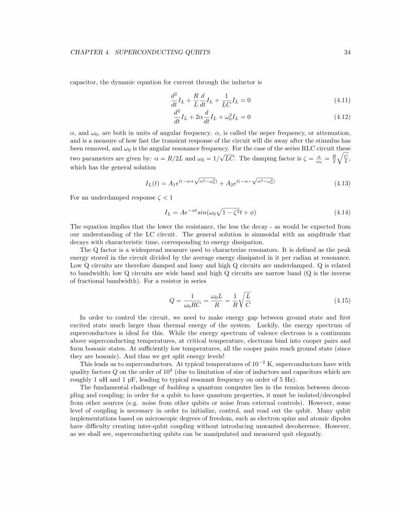
CHAPTER 4. SUPERCONDUCTING QUBITS 34
capacitor, the dynamic equation for current through the inductor is
d2
dtIL +
R
L
d
dtIL +
1
LCIL = 0 (4.11)
d2
dtIL + 2α
d
dtIL + ω2
0IL = 0 (4.12)
α, and ω0, are both in units of angular frequency. α, is called the neper frequency, or attenuation,and is a measure of how fast the transient response of the circuit will die away after the stimulus hasbeen removed, and ω0 is the angular resonance frequency. For the case of the series RLC circuit these
two parameters are given by: α = R/2L and ω0 = 1/√LC. The damping factor is ζ = α
ω0= R
2
√CL ,
which has the general solution
IL(t) = A1et(−α+
√α2−ω2
0) +A2et(−α−
√α2−ω2
0) (4.13)
For an underdamped response ζ < 1
IL = Ae−αtsin(ω0
√1− ζ2t+ φ) (4.14)
The equation implies that the lower the resistance, the less the decay - as would be expected fromour understanding of the LC circuit. The general solution is sinusoidal with an amplitude thatdecays with characteristic time, corresponding to energy dissipation.
The Q factor is a widespread measure used to characterize resonators. It is defined as the peakenergy stored in the circuit divided by the average energy dissipated in it per radian at resonance.Low Q circuits are therefore damped and lossy and high Q circuits are underdamped. Q is relatedto bandwidth; low Q circuits are wide band and high Q circuits are narrow band (Q is the inverseof fractional bandwidth). For a resistor in series
Q =1
ω0RC=ω0L
R=
1
R
√L
C(4.15)
In order to control the circuit, we need to make energy gap between ground state and firstexcited state much larger than thermal energy of the system. Luckily, the energy spectrum ofsuperconductors is ideal for this. While the energy spectrum of valence electrons is a continuumabove superconducting temperatures, at critical temperature, electrons bind into cooper pairs andform bosonic states. At sufficiently low temperatures, all the cooper pairs reach ground state (sincethey are bosonic). And thus we get split energy levels!
This leads us to superconductors. At typical temperatures of 10−2 K, superconductors have withquality factors Q on the order of 104 (due to limitation of size of inductors and capacitors which areroughly 1 nH and 1 pF, leading to typical resonant frequency on order of 5 Hz).
The fundamental challenge of building a quantum computer lies in the tension between decou-pling and coupling; in order for a qubit to have quantum properties, it must be isolated/decoupledfrom other sources (e.g. noise from other qubits or noise from external controls). However, somelevel of coupling is necessary in order to initialize, control, and read out the qubit. Many qubitimplementations based on microscopic degrees of freedom, such as electron spins and atomic dipoleshave difficulty creating inter-qubit coupling without introducing unwanted decoherence. However,as we shall see, superconducting qubits can be manipulated and measured quit elegantly.
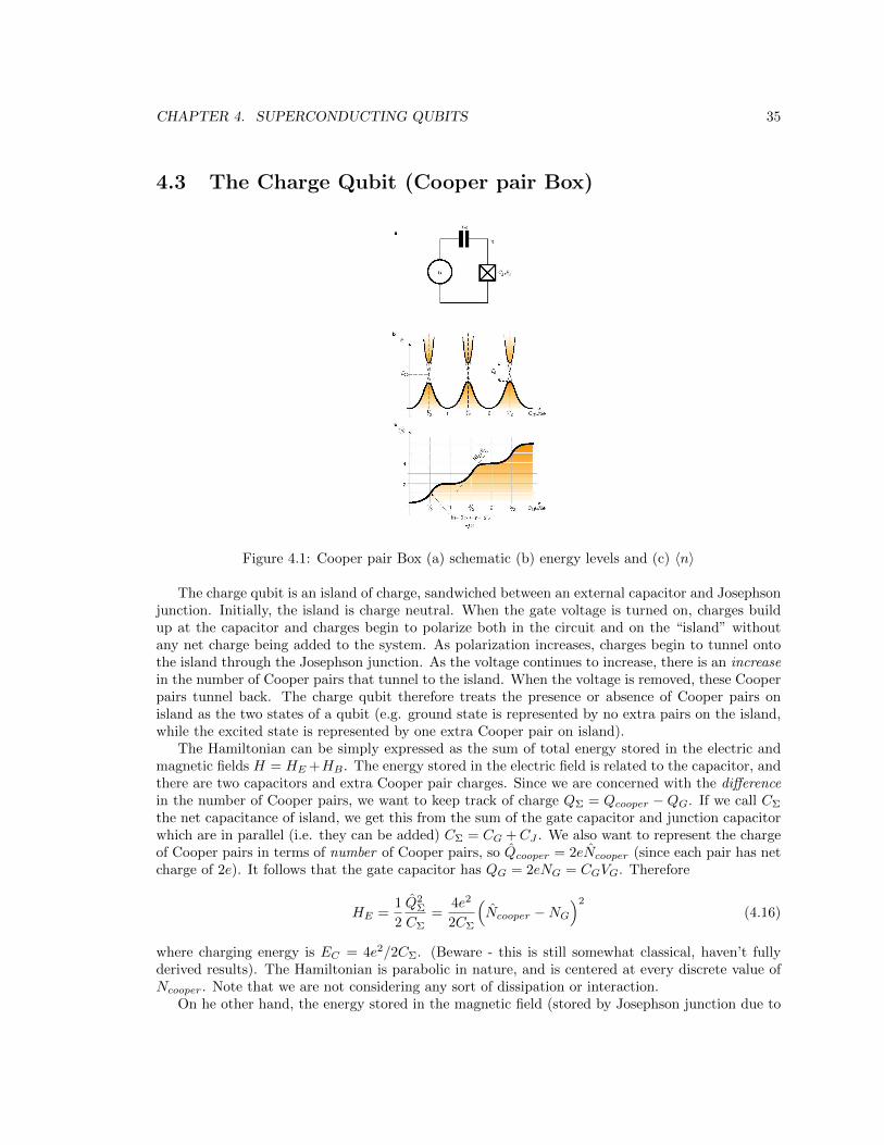
CHAPTER 4. SUPERCONDUCTING QUBITS 35
4.3 The Charge Qubit (Cooper pair Box)
Figure 4.1: Cooper pair Box (a) schematic (b) energy levels and (c) 〈n〉
The charge qubit is an island of charge, sandwiched between an external capacitor and Josephsonjunction. Initially, the island is charge neutral. When the gate voltage is turned on, charges buildup at the capacitor and charges begin to polarize both in the circuit and on the “island” withoutany net charge being added to the system. As polarization increases, charges begin to tunnel ontothe island through the Josephson junction. As the voltage continues to increase, there is an increasein the number of Cooper pairs that tunnel to the island. When the voltage is removed, these Cooperpairs tunnel back. The charge qubit therefore treats the presence or absence of Cooper pairs onisland as the two states of a qubit (e.g. ground state is represented by no extra pairs on the island,while the excited state is represented by one extra Cooper pair on island).
The Hamiltonian can be simply expressed as the sum of total energy stored in the electric andmagnetic fields H = HE +HB . The energy stored in the electric field is related to the capacitor, andthere are two capacitors and extra Cooper pair charges. Since we are concerned with the differencein the number of Cooper pairs, we want to keep track of charge QΣ = Qcooper −QG. If we call CΣ
the net capacitance of island, we get this from the sum of the gate capacitor and junction capacitorwhich are in parallel (i.e. they can be added) CΣ = CG +CJ . We also want to represent the chargeof Cooper pairs in terms of number of Cooper pairs, so Qcooper = 2eNcooper (since each pair has netcharge of 2e). It follows that the gate capacitor has QG = 2eNG = CGVG. Therefore
HE =1
2
Q2Σ
CΣ=
4e2
2CΣ
(Ncooper −NG
)2
(4.16)
where charging energy is EC = 4e2/2CΣ. (Beware - this is still somewhat classical, haven’t fullyderived results). The Hamiltonian is parabolic in nature, and is centered at every discrete value ofNcooper. Note that we are not considering any sort of dissipation or interaction.
On he other hand, the energy stored in the magnetic field (stored by Josephson junction due to
CHAPTER 4. SUPERCONDUCTING QUBITS 36
its inductor-like properties) is HB = −EJ0 cos δ
H = EC
(Ncooper −NG
)2
− EJ0 cos δ = EC
(− i d
dδ−NG
)2
− EJ0 cos δ (4.17)
Rewritten in the charge number basis as
H =∑N
[EC(Ncooper −NG)2 |N〉 〈N | − 1
2EJ0(|N〉 〈N + 1|+ |N + 1〉 〈N |)
](4.18)
(4.19)
If we make the two level approximation (i.e. assume that we only care about the lowest two) suchthat N = 0, 1, we can rewrite the Hamiltonian in terms of the familiar Pauli spin matrices,
H = −1
2EC(1− 2NG)σz −
1
2EJ0 σx (4.20)
and solve for energy eigenvalues3
E± = ±1
2
√E2C + E2
J0+ 4NGE2
C(NG − 1) (4.21)
What we see is that the magnetic component of Hamiltonian proportional to EJ creates energygaps at degeneracy points! Gap size between ground and first excited state is EJ , and thisenergy decreases with each level. This, of course, is anharmonic and allows for precise controlof transitions! More importantly, EC is a function of the voltage, while Ej is a function of theflux. These correspond to effective magnetic fields in the z-direction and x-direction respectively.Therefore, we have effectively created a tunable atom!
4.3.1 Tuning Junction
The relevant tuning parameters in the Hamiltonian are the charging energy EC , the number ofgate charges NG and the Josephson energy EJ . EC is inversely proportional to net capacitance onisland, so we could add more capacitors to change capacitance. Since NG is proportional to theexternally applied voltage, tuning the voltage changes NG. While the Josephson energy EJ canbe manufactured to specification (e.g. surface area and thickness of Josephson substrate). Finally,the phase difference depends on magnetic flux through junction; two junctions in parallel changedependence of cosine term in EJ according to magnetic flux through loop of junctions.
4.3.2 Manipulation
The next question is, how driving force will affect qubit? If we tune the frequency of the drivingoscillator near the transition frequency of system, we would expect system to transition from groundstate to first excited state (corresponding to an X-gate)
Using the rotating wave approximation (see Appendix), we can derive the following Hamiltonianthat relates the driving frequency and the driving phase to the Pauli spin matrices
Hrot =1
2(ωq − ωd)σz +
1
2A(cosφσx + sinφσy) (4.22)
3Note that the above Hamiltonian differs slightly depending on particular circuit
CHAPTER 4. SUPERCONDUCTING QUBITS 37
The long and short of it is that the frequency of the driving voltage controls z-axis rotations, andthe phase of the driving voltage controls x and y-axis rotations!
4.3.3 Qubit-Qubit Coupling and Quantum Non-Demolition (QND) Read-out
The final piece to the superconducting qubit schematic is qubit measurement. This is done bycoupling the qubit to a resonator and measuring the effective resonant frequency. The mathematicsis somewhat involved and draws from the well researched field of cavity quantum electrodynamics(cavity QED). The goal is to convert the Hamiltonian of the resonator qubit system into the formof the Jaynes-Cummings Hamiltonian, which is a template Hamiltonian used in qavity QED. TheJaynes-Cummings Hamiltonian looks like
HJaynes−Cummings = hω
(a†a+
1
2
)+
1
2hωσz +
1
2hg
(aσ+ + a†σ−
)(4.23)
where ωc is the frequency of the mode of oscillation of the radiation in the cavity, ωa is the transitionfrequency of the atom trapped in the cavity, g is the coupling factor, and σ± are the raising andlowering operators of the atom. If we ignore the high frequencies (since contributions to evolution ofthe system are too fast for consideration), we can rewrite original Hamiltonian into Jaynes-Cummingsform
H = hωr
(a†a+
1
2
)+
1
2EJ σz +
1
2hg
(aσ+ + a†σ−
)(4.24)
with
g = ECCG2e
√hωr2C
(4.25)
where CG is the capacitance of the capacitor in the qubit, and C is the capacitance of the capacitorin the LC resonator circuit. Coupling between resonator and qubit take energy from resonator andgive to qubit (ασ+) or vice versa.
In order to actually measure the qubit, we detune the resonant frequency of the resonator and thequbit so that when a signal is sent to qubit through the resonator, the resonator is hardly perturbed.We simplify the Hamiltonian further (since it is weakly coupled) and fin that the effective frequencyof the resonator ωr when coupled to the qubit, is dependent on the state of the qubit. Oncethe resonator and qubit are detuned (dispersive regime), we can measure ωr to determine stateof qubit without disturbing qubit (i.e. Quantum Non Demolition). It is then possible to performbasic spectroscopy on resonator, and hence measure the system. We mention here that qubit-qubitcoupling differs between various physical implementations, but are usually similar to the methodsdescribed above. See the Girvin chapter [16] or the review article by Devoret et al. [17] for moredetails.
Chapter 5
The Physics of Decoherence
Decoherence is the loss of coherence or ordering of the phase angles between the components of asystem in a quantum superposition due to energy dissipation and/or pure dephasing. This representsone of the most difficult and unique challenges to quantum computing, as the entire theory requiresthat coherence times are better than particular fault tolerant thresholds. Fortunately, decoherencetheory allows us to understand which parameters are important for improving coherence times, andit does not seem like there are any theoretical principles that limit coherence times below the faulttolerant thresholds.
In this chapter, the theory is developed carefully, first with toy models and then with the canonicalspin-boson model and spin bath model. We also emphasize how coherence times might be improvedfrom a mathematical perspective.
Density matrices and reduced density matrices play an important role in decoherence theory. Thisis because, when entanglement occurs (say, between the system of interest and the environment), wecannot describe the entangled system in terms of a single quantum state vector (see section 2.1.6).However, the measurement statistics of such entangled systems can be elegantly described withreduced density matrices. The following exposition on density matrices and decoherence modelsroughly follows Schlosshauer, Chapters 2-5 [37]. Maximilian Schlosshauer’s Decoherence and theQuantum to Classical Transition is an extremely well written book that covers the above topicsin much more depth. Roland Omnes’ well known book The Interpretation of Quantum Mechanics[36] is also a good introduction to the general subject of decoherence and the role it plays in theinterpretation of quantum mechanics. Finally, Joos Zeh and others wrote a well regarded (and moreadvanced) volume on the subject called Decoherence and the Appearance of a Classical World inQuantum Theory [27].
5.1 Density Matrices
We begin with a density matrix of a pure state (i.e. unentangled). We can define the densityoperator ρ corresponding to a pure state |ψ〉 as ρ ≡ |ψ〉 〈ψ|, which is the projection operator ontothe state |ψ〉. If we reexpress |ψ〉 as a superposition of basis states |φi〉 such that |ψ〉 =
∑i ci |φi〉
with a corresponding density operator
ρ = |ψ〉 〈ψ| =∑ij
cic∗j |φi〉 〈φj | (5.1)
38
CHAPTER 5. THE PHYSICS OF DECOHERENCE 39
This can be written in matrix form, and is called the density matrix
ρij = cic∗j 〈φi|ψ〉〈ψ|φj〉 = cic
∗j 〈φi|ρ|φj〉 (5.2)
ρ =
c1c∗1〈φ1|ρ|φ1〉 c1c
∗2〈φ1|ρ|φ2〉 . . .
c2c∗1〈φ2|ρ|φ1〉 c2c
∗2〈φ2|ρ|φ2〉
.... . .
(5.3)
While the i = j terms are called the diagonal terms, the i 6= j terms are called the off-diagonalterms, or interference terms. These interference terms are the embodiment of coherent superpositiondiscussed in section 2.1.2. It is important to keep in mind, however, that these interference termsshould always be understood in terms of a particular basis (in this case |φi〉. A basis in which thedensity matrix becomes diagonal always exists, and there will be no interference in this basis. AsSchlosshauer emphasizes, we should not assume that a diagonal density matrix implies a system that“does not have quantum properties” or “behaves classically.”1 Note that the two ways of describingthe system (either as a pure state |ψ〉 or as a pure state density operator ρ = |ψ〉 〈ψ|) are entirelyequivalent formally and physically.
The density matrix formalism turns out to be much more useful when dealing with mixed states,or statistical ensembles of several pure states. In such scenarios, insufficient information is knownabout the system - it is in a pure state, but the observer does not know which pure state. We cantherefore ascribe probabilities pi to each of the pure states |ψi〉. The density matrix is the quantum-mechanical analogue to a phase-space probability measure (probability distribution of position andmomentum) in classical statistical mechanics. The mixed state itself represents a classical ensemble,where the origin of the probabilities is purely classical. Supposing that a quantum system may befound in state |ψ1〉 with probability p1, or in state |ψ2〉 with probability p2, and so on, the densityoperator for this system is
ρ =∑i
pi|ψi〉〈ψi| (5.4)
where |ψi〉 need not be orthogonal and∑i pi = 1. By choosing an orthonormal basis |um〉, one
may resolve the density operator into a density matrix or density operator:
ρmn =∑i
pi〈um|ψi〉〈ψi|un〉 = 〈um|ρ|un〉, ρ =∑mn
|um〉ρmn〈un| (5.5)
For an operator O, which describes an observable O of the system, the expectation value 〈O〉 isgiven by
〈O〉 =∑i
pi〈ψi|O|ψi〉 =∑i
pi 〈ψi|un〉 〈un| O |um〉 〈um|ψi〉 (5.6)
=∑mn
〈um|ρ|un〉〈un|O|um〉 =∑mn
ρmnOnm = Tr(ρO) (5.7)
where the trace operation Tr acting on an operator O in the basis |ψi〉 is defined as Tr(O) ≡∑i 〈ψi| O |ψi〉 (i.e. the sum of the diagonal elements). In other words, the expectation value of O for
the mixed state is the sum of the expectation values of O for each of the pure states |ψi〉 weightedby the probabilities pi and can be computed as the trace of the product of the density matrix with
1Schlosshauer, p. 35 [37].
CHAPTER 5. THE PHYSICS OF DECOHERENCE 40
the matrix representation of O in the same basis. We also note here that for an entangled system,the density operator ρ of the composite system cannot be written as the tensor product of the twosubsystems ρ1 ⊗ ρ2.
Now the real motivation to introduce this formalism is to use reduced density matrices todescribe the dynamics of an open quantum system - a system where the environment is significantlyinfluencing the quantum system of interest. If a quantum system has two or more subsystems thatare entangled, then each subsystem must be treated as a mixed state even if the complete system isin a pure state. The basic example is for a quantum system A entangled with a quantum system B.The combined quantum system AB may be pure, but we can only access (i.e. perform measurementson) one of the systems, A. The most appropriate way to express all the information available to theobserver of system A is with the reduced density matrix
ρA ≡ TrBρ (5.8)
where TrB is the trace performed using the orthonormal basis of the Hilbert space HB of system B,or the partial trace. We can interpret this as averaging over the observed degrees of freedom of theunobservable system B. Importantly, this definition seems to hint that the system B plays some rolein the dynamics of AB, and that this is part of the outcome of A when system A is observed.
In order to derive this reduced density matrix, consider an entangled state of systems A and B
|Ψ〉 =1√2
(|a1〉 |b1〉+ |a2〉 |b2〉) (5.9)
where |ai〉 , |bi〉 are arbitrary normalized but not necessarily orthogonal states of A and B. The purestate density matrix (i.e. of the total system AB, which is pure) is:
ρ = |Ψ〉 〈Ψ| = 1
2
2∑ij=1
|ai〉 〈aj | ⊗ |bi〉 〈bj | (5.10)
This bipartite density matrix isn’t particularly insightful.2 We want to calculate expectation valuesfor A-observables, which we call O = OA ⊗ IBwith |ψk〉 and |φl〉 as orthonormal bases of theHilbert spaces HA and HB of A and B. Since the expectation value 〈O〉 of any observable can becomputed using the trace rule (5.6), we can write
〈O〉 = Tr(ρO) =∑kl
〈φl| 〈ψk| ρ(OA ⊗ IB
)|ψk〉 |φk〉 (5.11)
=∑k
〈ψk|(∑l=1
〈φl| ρ |φl〉)OA |ψk〉 (5.12)
=∑k
〈ψk| (TrBρ)OA |ψk〉 (5.13)
= TrA
((TrBρ)OA
)= TrA
(ρAOA
)(5.14)
2This can be expressed as 12
(|a1〉 〈a1| ⊗ |b1〉 〈b1|+ |a2〉 〈a1| ⊗ |b2〉 〈b1|+ |a1〉 〈a2| ⊗ |b1〉 〈b2|+ |a2〉 〈a2| ⊗ |b2〉 〈b2|
)or alternatively as 1
2
(|a1b1〉 〈a1b1|+ |a2b2〉 〈a1b1|+ |a1b1〉 〈a2b2|+ |a2b2〉 〈b2b2|
)
CHAPTER 5. THE PHYSICS OF DECOHERENCE 41
For the bipartite state, the reduced density operator is
ρA =1
2
2∑ij=1
|ai〉 〈aj | 〈bj |bi〉 (5.15)
=1
2|a1〉 〈a1|+
1
2|a2〉 〈a2|+
1
2
(|a1〉 〈a2| 〈b2|b1〉+ |a2〉 〈a1| 〈b1|b2〉
)(5.16)
Where the two terms in the brackets are the off diagonal interference terms. It is clear that theinfluence of system B is interconnected with with off diagonal A terms. And here is the key - ifthe states |b1〉 and |b2〉 are orthogonal, then the off diagonal terms - and hence any indication ofinterference - vanish. This will become more evident in the next example.
Also note that this result can be generalized for entanglement between N subsystems:
ρi = Tr1,...,i−1,i+1,...,N (ρ), and 〈O〉 = Tr(ρO) = Tri(ρiOi) (5.17)
The insight here is that by tracing over all or a fraction of the degrees of freedom of the environment,we can obtain a complete and exhaustive description of the measurement statistics for the system ofinterest.
5.2 Simple Model for Decoherence
As an instructive example to build on the above result, let us consider a two-qubit system wherethe second qubit is “environmental noise” B. The interaction Hamiltonian between two, two-levelsystems is described by the Heisenberg Hamiltonian equation 2.12 (with h = 1)
H =J
4σ(A)z ⊗ σ(B)
z (5.18)
where J is simply a coupling constant. Starting with the product state |Ψ(t0)〉 = |+〉A⊗|+〉B = |++〉,we let the system unitarily evolve with operator U(t) = e−iHt (equation 2.2) and then perform thetrace operation on the B-qubit to understand how the A-qubit evolved (and how it was influencedby the B-qubit). We can write the density operator ρA
ρA = |+〉A 〈+|A =1
2(|0〉 〈0|+ |1〉 〈1|+ |0〉 〈1|+ |1〉 〈0|) (5.19)
and the density matrix as
ρA =1
2
(1 11 1
)(5.20)
at time t we have
|Ψ(t)〉 = U(t) |+〉A |+〉B = e−iJtσAσB/2 |+〉 |+〉 (5.21)
(5.22)
The state of the A-qubit at time t is given by
ρ1(t) = Tr(|Ψ(t)〉 〈Ψ(t)|) =1
2
(1 cos(Jt/2)
cos(Jt/2) 1
)(5.23)
CHAPTER 5. THE PHYSICS OF DECOHERENCE 42
The algebra for equation 5.23 is a bit cumbersome3. It is evident that while the diagonal elementsare constant, the off-diagonal elements change with time. This means that the coherence is periodi-cally completely lost and then completely regained (albeit with sign changes) at intervals of π/J . Thecoherence is regained when The real consequences of this changing coherence are highlighted in thenext example.
In 1982, Wojciech Zurek created one of the first basic models to illustrate basic features ofenvironment induced decoherence [43]. The model consists of a two level quantum system S linearlycoupled to an environment E that is comprised of N other quantum two level systems (this is ageneralization of the above toy model). Although it is overly simplified for most purposes, it can beapplied to certain real, physical systems.4 Two basis states of S are |0〉 and |1〉 while the basis statesof the N two level systems of environment E are |↑〉i , |↓〉i where i = 1, 2, ...N . The total system-environment combination is a 2N+1 dimensional tensor product Hilbert space H = HS ⊗ HE1...N .Assuming that the interaction Hamiltonian Hint dominates the evolution (i.e. ignoring intrinsicdynamics of each system), we have
H =1
2σz ⊗
(g1σ
(1)z ⊗ I2,3,...N + g2σ
(2)z ⊗ I1,3,...N + ...
)(5.24)
=1
2σz ⊗
( N∑i=1
giσ(i)z
⊗i′ 6=i
Ii′
)(5.25)
=1
2σz ⊗ E (5.26)
Each element in the environment couples to the central system S, but they do not couple witheach other (the identity is only necessary when i′ 6= i, and is implicit in E). The qubit coupleslinearly through z-spin component to each of the environmental spins, where gifor i = 1, 2, ...N isthe coupling strength, while the Hamiltonian is in diagonal form. Since the Hamiltonian commutes,it is a conserved quantity and no energy is exchanged and therefore no dissipation needs to occur.We can describe the energy eigenstates of the environment part E of the Hamiltonian as |n〉 =|↑〉1 |↓〉2 ... |↑〉N , and associate energy εn with each eigenstate |n〉
εn =
N∑i=1
(−1)nigi (5.27)
where we define ni = 1 if ith environmental spin is in the down state |↓〉 and ni = 0 if ith environ-mental spin is in the up state |↑〉 any arbitrary pure state of SE can be represented as:
|Ψ〉 =
2N−1∑n=0
(cn |0〉 |n〉+ dn |1〉 |n〉) (5.28)
3We can notice that the eigenvectors of the 4×4 matrix σz⊗σz are |00〉 , |11〉 , |01〉 , |10〉 with eigenvalues 1, 1,−1,−1
respectively. Remembering that the function of an operator can be expressed as f(A) =∑i f(λi) |ai〉 〈ai|, where λi
is an eigenvalue and |ai〉 is an eigenvector, we can write
e−iJtσz σz/2 |+〉 |+〉 =[e−iJt/2(|00〉 〈00|+ |11〉 〈11|) + eiJt/2(|01〉 〈10|+ |10〉 〈01|)
]|++〉 etc.
4Schlosshauer p. 90 [37]
CHAPTER 5. THE PHYSICS OF DECOHERENCE 43
Assuming that S and E are uncorrelated at t = 0,
|Ψ〉 = (a |0〉+ b |1〉)2N−1∑n=0
cn |n〉 (5.29)
As above, the time evolution of the total system SE can be expressed as
|Ψ(t)〉 = e−iHt |Ψ(0)〉 = a |0〉 |E0(t)〉+ b |1〉 |E1(t)〉 (5.30)
|E0(t)〉 =
2N−1∑n=0
cne−iεnt/2 |n〉 (5.31)
Already we can see that the basis states |0〉 , |1〉 of S are correlated with the relative states |E0(t)〉 , |E1(t)〉of the environment E . The smaller the overlap between 〈E1(t)|E0(t)〉 , the more information is en-coded in the environment that distinguishes between states |0〉 and |1〉. 〈E1(t)|E0(t)〉 is interpretedas the decoherence factor r(t), given by
r(t) ≡ 〈E1(t)|E0(t)〉 ≡2N−1∑n=0
|cn|2e−iεnt (5.32)
Taking the trace in the |0〉 , |1〉 basis
ρS(t) = TrE ρ(t) ≡ TrE |Ψ(t)〉 〈Ψ(t)| (5.33)
= |a|2 |0〉 〈0|+ |b|2 |1〉 〈1|+ ab∗r(t) |0〉 〈1|+ a∗br∗(t) |1〉 〈0| (5.34)
Finally, we see that if r(t) −→ 0, the interference terms disappear. Hence r(t) describes localdamping of interferences between |0〉 and |1〉.
But how does r(t) change overtime, and how is it affected by the number of spins N in theenvironment? Cucchietti, Paz and Zurek [14] were able to show that:
1. The degree of suppression of coherence scales exponentially with size N of the environment
2. For sufficiently large N , r(t) follows an approximately Gaussian decay with time r(t) ≈ e−Γ2t2 ,where Γ2 is a decay constant determined by the initial state of the environment and thedistribution of couplings gi
3. As long as the number of degrees of freedom of the environment E is finite, there exists acharacteristic recurrence time for which the decoherence factor will return to it’s initial valueof one (this is because equation 5.32 is a sum of periodic functions, which is in turn periodic).In physically relevant situations, the characteristic recurrence time is extremely long (and caneven exceed the lifetime of the universe). Thus even with this simple model, loss of coherenceis for all practical purposes irreversible.
4. There are a few unique states/boundary conditions: for example, if the each element in theenvironment system was initially in the 1√
2(|↑〉 + |↓〉), then r(t) would be cosN (gt), which is
periodic with frequency g/2π. However these do not usually apply in physical situations.
This particular model highlights a few important points. Most importantly, we see that including“the environment” in a model can essentially explain the quantum to classical transition. Why
CHAPTER 5. THE PHYSICS OF DECOHERENCE 44
don’t we see coherence at the macroscopic level? Because coherence is suppressed by environmentalinteractions. In addition, the interactions in this particular model were energy conserving - sodespite the fact that there was no energy exchanged/dissipated, decoherence did occur. The fact thatdecoherence can occur without energy dissipation makes it very clear that decoherence is a uniquelyquantum phenomenon. In the more “realistic” models we will see soon, of course, decoherenceusually does include dissipation.
5.3 Scattering Models
The next well known type of models are the scattering induced decoherence models. Althoughthe derivations are too lengthy for this context, a few comments are in order. Many of the ideasof open quantum systems and environmentally induced decoherence were developed in the 1970sand 1980s. It is now understood that any interaction between a massive object and a particlemay lead to entanglement and hence decoherence. The larger the object, the larger the scatteringcross section, the faster the decoherence. Interestingly, scattering induced decoherence resolvesSchrodinger’s historical problem of describing particles as spatially extended waves. It is generallytaught in introductory physics courses that a free particle described by a locally spatialized wavepacket spreads out on very short timescales. For example, if we describe a free particle with the massof an electron (m ≈ 10−30 kg) as a gaussian wave packet with an initial width of 1 angstrom, unitarytime evolution spreads the wave packet to a width on the order of 1,000 km!5 The seminal paper byE. Joos and H.D. Zeh in 1985 [26] showed for the first time that ubiquitous scattering of photons,air molecules and other environmental particles effectively suppresses the coherent spreading of freeparticles on extremely short timescales. For more detail, see Omnes Chapter 7 [36] and SchlosshauerChapter 3.1 [37]. Ample references to original papers can be found there as well.
5.4 Canonical Decoherence Models
The beauty of decoherence theory is that it allows us to map complex systems onto canonical models.There are four main canonical models for open quantum systems, which are made up of two kindsof central systems and two kinds of environment systems:
• Central system S: The central system of interest is either modeled as (1) particles withcontinuous coordinates x and p (e.g. photons) or (2) as discrete, two level systems (TLS) (e.g.spin-1/2 particles)
• Environment E: The interacting environment can either be modeled as (1) a collection ofcontinuous harmonic oscillators, or as (2) a collection of discrete two level systems
The spin-boson model is a canonical model of a two level system coupled to an environment ofharmonic oscillators. Generally, the model is solved with an arbitrary choice of parameters, and then“fit” to physically relevant situations by filling in parameters. Often times the same canonical modelwill be unique in different regimes. The purpose of these next two sections is to provide an overviewof the two canonical decoherence models used for superconducting qubit theory and experiment.
Often times the two level central system is can be modeled as a particle confined to a doublewell potential - two energy minimums (excited and ground states) separated by a barrier. Hencethe Hamiltonian can consist of a simple excitation/relaxation term, as well as a tunneling term.6 It
5A free particle ψ(x, t = 0) = (√πσ)−1/2e−x
2/2σ2has probability density |ψ(x, t)|2 = (1/
√πσ(t))e−x
2/σ2(t). Thewidth of the wavepacket grows as σ(t) = σ[1 + h2t2/(m2σ4)]1/2 See Schlosshauer, p.119[37]
6The Hamiltonian of a tunneling term is H = −1/2∆0σx, which is simple a flip operator |e〉 → |g〉 or |g〉 → |e〉
CHAPTER 5. THE PHYSICS OF DECOHERENCE 45
is clear that qubits can be modeled as two level systems (TLS), and this is the most appropriatecentral system S. We’ve thus narrowed down the canonical models to the spin-boson model (withoscillator environments) and the spin-bath model (with spin environments). When do each of thesemodels apply?
Oscillator environments are essentially a quasicontinuum of delocalized bosonic field modes.When decoherence occurs due to oscillator environments, energy and coherence are effectively irre-versibly lost into the extended bosonic environment.7 Spin environments, on the other hand, areparticularly useful for modeling low temperature, superconducting experiments. This regime is dom-inated by local modes, such as paramagnetic spins, electronic impurities, tunneling charges, defects,nuclear spins, etc. Decoherence caused by these modes are confined to small regions in space. As weshall see with superconducting qubits, even small improvements in the number of material defectscan greatly improve coherence times.
The subfields of decoherence and open quantum systems have an extensive toolbox of rigorousmathematical objects (e.g. Schmidt decomposition, Wigner representation, Operator-Sum formal-ism, Master equations, Born Markov approximations, Lindbald form, Langevin equations). How-ever, simple versions of the spin-boson model and the spin-bath model can be analyzed without thismathematical heavylifting.8
5.5 Spin-Boson Model
For the purposes of this discussion, we will consider a simplified version of the model in which theHamiltonian of the spin system does not contain a tunneling term. Despite the fact that it is asimplified version, it still displays many of the characteristic features of decoherence.9
5.5.1 Set up
We begin with a Hamiltonian of the form
H = HS + HE + Hint (5.35)
The first term is the Hamiltonian of the central system S, defined as HS = 12ω0σz. ω0 is the
difference in energy between the basis states |0〉 and |1〉. Note that in the more extensive model, thetunneling term would be included in HS as well.
7Feynman and Vernon actually showed that the interaction with any environment can be linearly mapped onto asystem coupled to a an oscillator environment assuming that the interaction is weak and second-order perturbationtheory can be applied [20].
8Schlosshauer, again, does a fantastic job motivating and explaining much of this mathematical framework in [37]9Some interesting examples of physical models that make this simplifying assumption:
1. Unruh, William G. “Maintaining coherence in quantum computers.” Physical Review A 51.2 (1995): 992.
2. Palma, G. Massimo, Kalle-Antti Suominen, and Artur K. Ekert. “Quantum computers and dissipation.”Proceedings of the Royal Society of London A: Mathematical, Physical and Engineering Sciences. Vol. 452.No. 1946. The Royal Society, 1996.
3. Duan, Lu-Ming, and Guang-Can Guo. “Reducing decoherence in quantum-computer memory with all quantumbits coupling to the same environment.” Physical Review A 57.2 (1998): 737.
4. Reina, John H., Luis Quiroga, and Neil F. Johnson. “Decoherence of quantum registers.” Physical Review A65.3 (2002): 032326.
CHAPTER 5. THE PHYSICS OF DECOHERENCE 46
The second term is the Hamiltonian of the environment of harmonic oscillators, with the familiar
HE =∑i
(1
2mip2i +
1
2miω
2i q
2i
)(5.36)
where the bosonic mode i of the ith oscillator is defined by its natural frequency ωi, mass mi,position operator qi and momentum operator pi.
Finally, the third term describes the linear coupling between the two level system S and theenvironment E .
Hint = σz ⊗∑i
ciqi (5.37)
where the σz coordinate is coupled to the position coordinates qi of each harmonic oscillator withcoupling strengths ci. It is convenient to write the Hamiltonians in terms of the bosonic annihilatianand creation operators for each mode.
qi =
√1
2miωi
(ai + a†i
)(5.38)
pi = −i√miωi
2
(ai − a†i
)(5.39)
and dropping the vacuum-energy term∑i ωi/2 , we can rewrite the full Hamiltonian as
H =1
2ω0σz +
∑i
ωia†i ai + σz ⊗
∑i
(gia†i + g∗i ai
)(5.40)
As in the in simple spin model above (equation 5.24), the property[H, σz
]= 0 indicates that
there is a conserved quantity. In this case, there is no induced transition between the ground andexcited state of the two level system S (which would involve a σx operator), and hence no energydissipation (|e〉 → |g〉) or absorption (in the form of excitation |g〉 → |e〉). In addition, the populationsof the two energy levels are conserved quantities. This is therefore a model of decoherence withoutdissipation. In circumstances where the timescale for decoherence without dissipation is much shorterthan the timescale for energy relaxation, the above model suffices. Clearly the more complete modelwith the tunneling term allows for energy dissipation as well.
5.5.2 Solution
The strategy is to obtain a relatively workable expression for the time evolution operator. Unfortu-nately this involves more math than can appropriately fit here (the basic approach is to switch to theinteraction picture, write the time evolution operator U(t) as a time ordered product of operators,expand in terms of a Dyson series and then express U(t) in terms of a non time ordered evolutionoperator V (t)).
Making the usual assumption thatS and E are uncorrelated at time t = 0, we obtain the timeevolution:
CHAPTER 5. THE PHYSICS OF DECOHERENCE 47
|Ψ(t)〉 = V (t) |Ψ(0)〉 = V (t)(a |0〉+ b |1〉) |ΦE〉 (5.41)
= a |0〉∏i
D(λi(t)/2) |ΦE〉+ b |1〉∏i
D(−λi(t)/2) |ΦE〉 (5.42)
≡ a |0〉 |E+(t)〉+ b |1〉 |E−(t)〉 (5.43)
where D(λi(t)) is an operator that generates the evolution of the i-th environmental oscillator. Un-surprisingly, the form of the |Ψ(t)〉 is similar to that obtained in the simple spin-spin model insection 5.2, equation 5.30. In both cases, the states |0〉 , |1〉 of the central system S and the states|E+(t)〉 , |E−(t)〉 environment E are clearly and elegantly correlated. The specific forms of the states|E+(t)〉 , |E−(t)〉 of course depend on the initial state of the environment.
Environment in ground state: The first scenario to look at is the initial state of E in theenergy ground state |ΦE〉 =
∏i |E0〉i where i runs over all the environmental oscillators. This
can be likened to a measurement like process - the state of the environment |ΦE〉 gets shifted intothe states |E+(t)〉 , |E−(t)〉. And if the environment is sufficiently macroscopic, they are capable ofdiscriminating between the states |0〉 and |1〉. The coherence will be lost from the system, and theoff-diagonal elements in the reduced density matrix of the system (expressed in the basis |0〉 , |1〉)will disappear.
It can be shown that the decoherence factor is given by
r(t) = 〈E−(t)|E+(t)〉 = exp(−∑i
4|gi|2
ω2i
(1− cosωit))≈ exp
(−∑i
2|gi|2t2)
(5.44)
where the final approximation is for t much smaller than dynamical timescales ω−1i of the modes
(i.e. ωit 1, so the cosine can be approximated to cos(ωit) ≈ 1− 12ω
2i t
2). This final approximationgives a gaussian decay of coherence between the states |0〉 and |1〉.
Environment in thermal equilibrium: This is the more general case, where the environmen-tal oscillator is in a thermal state.
If the environment is sufficiently large, we can assume a continuous density of environmentalmodes.
We can then analyze the decoherence factor in terms of a sum over the discrete couplings gito a continuous description by means of the spectral density J(ω).10 The typical approach is toconsider spectral density that is ohmic for sufficiently small frequencies J(ω) ∝ ω that has a smoothhigh-frequency cutoff quantified by Λ. Integrating over ω, we get a result that can be separated intotemperature dependent and temperature independent terms
Γ(t) = Γfluc(t) + Γtherm(t) (5.45)
where Γfluc(t) = − 12 ln(1 + Λ2t2) and Γtherm(t) ≈ − ln(sinh(πkBTt)/πkBTt). Note that Γfluc is
independent of the temperature, but sensitive to the cutoff frequency, while Γtherm is dependent on
10This replaces the discrete sum in the modes for J(ω) with an (often phenomenologically motivated) continuousfunction of the environmental frequencies ω. Usually, the frequency dependence of J(ω) is taken to follow a power-law dependence of the form J(ω) ∝ ωα. The most common choice for the exponent α is α = 1, such that J(ω)increases linearly with ω. This type of spectral density is called ohmic (the nomenclature has its origin in an analysisof dissipative effects in the spin boson model). Other, less important examples include subohmic spectral densitiescharacterized by α < 1 and supraohmic spectral densities for which α > 1. Schlosshauer p. 188 [37]
CHAPTER 5. THE PHYSICS OF DECOHERENCE 48
the temperature, and independent of Λ. It can be shown that at short and extremely short timeregimes, decoherence is entirely due to quantum vacuum fluctuations. It can also be shown that forlong-time regimes (much larger than the typical thermal fluctuation time), the decoherence factorr(t) decays exponentially on a timescale set by the thermal correlation time (kBT )1. It is clear fromthis very general model that coherence times can be improved by decreasing temperature, an obviousbut important result. Schlosshauer has an extensive derivation of the above results in Chapter 5 of[37].
5.5.3 Full Spin-Boson Model
Shnirman, Makhlin and Schon review the full spin boson model and apply it to superconductingcharge qubits in their 2002 paper Noise and Decoherence in Quantum Two-Level Systems [38], andalso summarize what is known about relaxation and dephasing processes for spin-boson models withlinear coupling. The key difference from the previous model is the addition of the tunneling term∝ σx that makes the dynamics much more rich. Again, the motivating question is: how do we getfrom a model to an estimation of decoherence time?
With this model, there is a dephasing timescale τφ as well as a relaxation timescale τrelax thatcharacterizes how the diagonal entries tend to their thermal equilibrium. The decoherence ratesusing the Bloch-Redfield approximation are
Γrelax ≡ τ−1relax =
1
h2 sin2 θSX(ω = ∆E/h) (5.46)
Γφ ≡ τ−1φ =
1
2Γrelax +
1
h2 cos2 θSX(ω = 0) (5.47)
The “pure” dephasing rate Γ∗φ is defined as being ∝ cos2 θ and is entirely non-dissipative andhas no classical analogue. This leads to the often quoted relation
Γφ =1
2Γrelax + Γ∗φ (5.48)
which is sometimes also stated as
1
T2=
1
2T1− 1
Tφ(5.49)
In environment dominated regime, ∆E αkBT , the coupling to the bath is dominant part ofHamiltonian, and dephasing Γφ is much faster than relaxation Γrelax.
5.6 Spin-Bath Model
The spin-bath model, or spin-spin model, is extremely useful for describing defects in supercon-ducting states. This is the regime where decoherence correlated with temperature is weak anddecoherence correlated to two-level state local defects are significant. Without going into much de-tail, the model is similar to the simple spin-bath model we encountered at the beginning of thischapter except for the inclusion of a tunneling term. Unsurprisingly, this leads to significantly dif-ferent dynamics compared to the earlier static model. Schlosshauer Section 5.4.1 [37] discusses thismodel in detail, and McDermott [33] applies this to superconducting qubits.
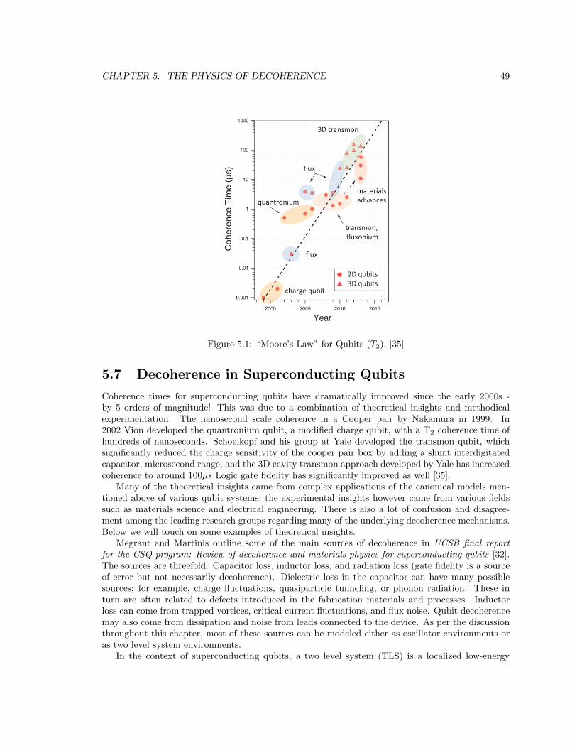
CHAPTER 5. THE PHYSICS OF DECOHERENCE 49
Figure 5.1: “Moore’s Law” for Qubits (T2), [35]
5.7 Decoherence in Superconducting Qubits
Coherence times for superconducting qubits have dramatically improved since the early 2000s -by 5 orders of magnitude! This was due to a combination of theoretical insights and methodicalexperimentation. The nanosecond scale coherence in a Cooper pair by Nakamura in 1999. In2002 Vion developed the quantronium qubit, a modified charge qubit, with a T2 coherence time ofhundreds of nanoseconds. Schoelkopf and his group at Yale developed the transmon qubit, whichsignificantly reduced the charge sensitivity of the cooper pair box by adding a shunt interdigitatedcapacitor, microsecond range, and the 3D cavity transmon approach developed by Yale has increasedcoherence to around 100µs Logic gate fidelity has significantly improved as well [35].
Many of the theoretical insights came from complex applications of the canonical models men-tioned above of various qubit systems; the experimental insights however came from various fieldssuch as materials science and electrical engineering. There is also a lot of confusion and disagree-ment among the leading research groups regarding many of the underlying decoherence mechanisms.Below we will touch on some examples of theoretical insights.
Megrant and Martinis outline some of the main sources of decoherence in UCSB final reportfor the CSQ program: Review of decoherence and materials physics for superconducting qubits [32].The sources are threefold: Capacitor loss, inductor loss, and radiation loss (gate fidelity is a sourceof error but not necessarily decoherence). Dielectric loss in the capacitor can have many possiblesources; for example, charge fluctuations, quasiparticle tunneling, or phonon radiation. These inturn are often related to defects introduced in the fabrication materials and processes. Inductorloss can come from trapped vortices, critical current fluctuations, and flux noise. Qubit decoherencemay also come from dissipation and noise from leads connected to the device. As per the discussionthroughout this chapter, most of these sources can be modeled either as oscillator environments oras two level system environments.
In the context of superconducting qubits, a two level system (TLS) is a localized low-energy
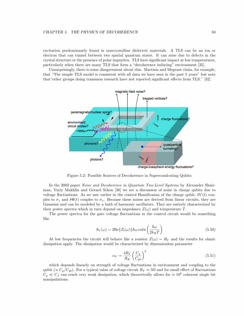
CHAPTER 5. THE PHYSICS OF DECOHERENCE 50
excitation predominantly found in noncrystalline dielectric materials. A TLS can be an ion orelectron that can tunnel between two spatial quantum states. It can arise due to defects in thecrystal structure or the presence of polar impurites. TLS have significant impact at low temperatures,particularly when there are many TLS that form a “decoherence inducing” environment [35].
Unsurprisingly, there is some disagreement about this. Martinis and Megrant claim, for example,that “The simple TLS model is consistent with all data we have seen in the past 5 years” but notethat“other groups doing transmon research have not reported significant effects from TLS.” [32]
Figure 5.2: Possible Sources of Decoherence in Supercondcuting Qubits
In the 2002 paper Noise and Decoherence in Quantum Two-Level Systems by Alexander Shnir-man, Yuriy Makhlin and Gerard Schon [38] we see a discussion of noise in charge qubits due tovoltage fluctuations. As we saw earlier in the control Hamiltonian of the charge qubit, δV (t) cou-ples to σz and δΦ(t) couples to σx. Because these noises are derived from linear circuits, they areGaussian and can be modeled by a bath of harmonic oscillators. They are entirely characterized bytheir power spectra which in turn depend on impedance Z(ω) and temperature T .
The power spectra for the gate voltage fluctuations in the control circuit would be somethinglike
SV (ω) = 2ReZt(ω)hω coth
(hω
2kBT
)(5.50)
At low frequencies the circuit will behave like a resistor Z(ω) = RV and the results for ohmicdissipation apply. The dissipation would be characterized by dimensionless parameter
αV =4RVRK
(CgCqb
)2
(5.51)
which depends linearly on strength of voltage fluctuations in environment and coupling to thequbit (∝ Cg/Cqb). For a typical value of voltage circuit RV ≈ 5Ω and for small effect of fluctuationsCg CJ can reach very weak dissipation, which theoretically allows for ≈ 106 coherent single bitmanipulations.
CHAPTER 5. THE PHYSICS OF DECOHERENCE 51
In the same paper, they begin to discuss stronger sources of noise: background charge fluc-tuations. They claim that they can be either modeled as two-state quantum system bath, or asapproximate oscillator bath with the appropriate spectrum, but do not discuss much further.
In the 2008 paper Materials Origins of Decoherence in Superconducting Qubits by Robert Mc-Dermott [33], he states that for defect energies larger than kBT , TLS defects behave like a “spinbath” in the quantum regime, and that the spin physics gives rise to unusual properties such asenhanced dielectric loss at low temperature and low microwave drive power. On the other hand,defects with energies less than kBT produce low-frequency charge and dielectric noise. Hence thequantum TLS contribute to qubit energy relaxation, while the thermal TLS contribute to dephasing.
Just as resonant a magnetic field can induce transitions in a system of spins immersed in a strongstatic magnetic field, resonant electric fields can couple to TLS with an electric dipole moment,including transitions and dissipation. The loss tangent tan δ of the amorphous dielectric decreasesdue to population of the TLS excited state. However, as thermal or external microwave transitionssaturate the TLS, the dielectric becomes transparent to resonant irradiation and the loss decreases
The dielectric loss of TLS can influence the qubit T1time in two ways: (1) lossy dielectrics incor-porated in the wiring external to the qubit junction contribute a fraction α to the qubit capacitance,and (2) in the case of a large qubit junction with area 100µm2 the tunnel barrier itself containsa quasicontinuum of resonant TLS and dissipation from these states can induce qubit relaxation.Interestingly, at millikelvin temperatures and at low microwave drive powers, the integral qualityfactor of the tank is the inverse of the intrinsic loss tangent of the capacitor dielectric Qi = 1/ tan δi.It is clear that the capacitance shunting the qubit junction should be entirely free of low energydefect states. While a continuum of TLS in bulk dielectrics can lead to energy relaxation, couplingof the qubit to discrete TLS in the Josephson barrier can itself lead to the quantum coherent transferof energy between the qubit and the TLS, and result in fidelity loss.
McDermott concludes that in order to minimize fidelity loss due to TLS in the qubit tunnelbarrier, it is necessary to reduce the density of resonant TLS. This can done straightforwardly eitherby reducing the area of the Josephson junction or by improving the quality of barrier.
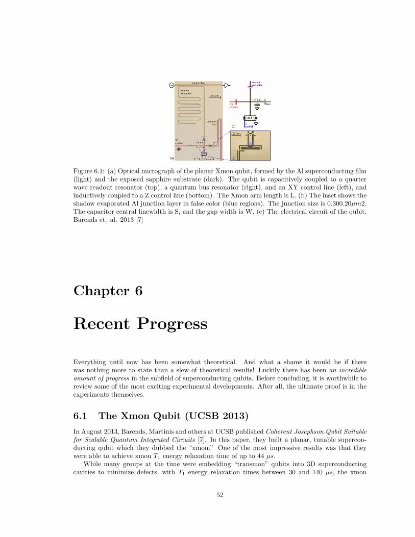
Figure 6.1: (a) Optical micrograph of the planar Xmon qubit, formed by the Al superconducting film(light) and the exposed sapphire substrate (dark). The qubit is capacitively coupled to a quarterwave readout resonator (top), a quantum bus resonator (right), and an XY control line (left), andinductively coupled to a Z control line (bottom). The Xmon arm length is L. (b) The inset shows theshadow evaporated Al junction layer in false color (blue regions). The junction size is 0.300.20µm2.The capacitor central linewidth is S, and the gap width is W. (c) The electrical circuit of the qubit.Barends et. al. 2013 [7]
Chapter 6
Recent Progress
Everything until now has been somewhat theoretical. And what a shame it would be if therewas nothing more to state than a slew of theoretical results! Luckily there has been an incredibleamount of progress in the subfield of superconducting qubits. Before concluding, it is worthwhile toreview some of the most exciting experimental developments. After all, the ultimate proof is in theexperiments themselves.
6.1 The Xmon Qubit (UCSB 2013)
In August 2013, Barends, Martinis and others at UCSB published Coherent Josephson Qubit Suitablefor Scalable Quantum Integrated Circuits [7]. In this paper, they built a planar, tunable supercon-ducting qubit which they dubbed the “xmon.” One of the most impressive results was that theywere able to achieve xmon T1 energy relaxation time of up to 44 µs.
While many groups at the time were embedding “transmon” qubits into 3D superconductingcavities to minimize defects, with T1 energy relaxation times between 30 and 140 µs, the xmon
52
CHAPTER 6. RECENT PROGRESS 53
was essentially a planar transmon that was much more versatile. Martinis saw it as a balanceof coherence, connectivity and relatively easy manufacturing. What was unique about this qubitwas that it was frequency tunable, meant that they could implement fast two-qubit gates (becausethere was not a concern of perturbing nieghboring qubits). They were also able to achieve theimportant benchmark of Control-Z in 25 ns. According to the paper, the xmon qubit “provideskey ingredient for implementing a surface code quantum computer.” They also found that energyrelaxation depends on qubit frequency.
In this paper they also investigated dependence of qubit coherence time on capacitor geometryusing six different designs - varying width of central line, gap width, and arm length. They foundthat overall energy relaxation time increases with width; the belief is that widening the capacitorreduced the surface participation of dipole moments residing on surface oxides ad interfaces. Theyalso noted that lower and upper bounds of T1 increasing with capacitor dimension seem to indicatethat defects reside within the capacitor. Also in the paper, they modeled decoherence mechanismarising from a sparse bath of weakly coupled (two level) defects.
How does the modular design work? Each arm has different function - a coplanar waveguideresonator for read out, a quantum bus resonator for coupling/entanglement, XY control for frequencycontrol and Z control for phase control. Three of the connections are made with coupling capacitor,and each coupling can be individually tuned and optimized. XY control can excite qubit in 10 ns,while T1 of XY control is 0.3 ms. Z-control - can rapidly detune on order of 1 ns, while T1 for z-controlis ≈ 30 ms. More arms can be added for connectivity. They also noted that the limit T2 = 2T1
was not reached, indicating additional dephasing. Also note that in the paper Qubit Architecturewith High Coherence and Fast Tunable Coupling [10] Chen, Cleland, Martinis and others were ableto demonstrate that the cross coupling effects between two xmon qubits could be made small forplanar integrated circuits while still allowing for multiqubit operations.
6.2 5-qubit Linear Array (UCSB 2014)
The next truly exciting experiment came in 2014. In the paper Superconducting Quantum Circuitsat the Surface Code Threshold for Fault Tolerance [8] Barends, Korotkov, Cleland, Martinis andothers announced that they had built a 5-qubit linear array using xmon qubits.
In this particular experiment, the UCSB group was able to demonstrate universal set of logicgates in a multi-qubit processor with single-qubit gate fidelity of 99.92% and two-qubit gate fidelity ofup to 99.4%. This is very good, as it places superconducting qubits at the fault tolerance thresholdfor surface code error correction. They were also able to construct a 5-qubit GHZ state. As theywrite in the paper: “The results demonstrate that Josephson quantum computing is a high fidelitytechnology with a clear path to scaling up to large-scale, fault tolerant quantum circuit.”
Among other technical achievements, the they were able to maintain controlled phase gate nearly40ns when two qubits were brought near resonance. This was with a dispersive measurement method;where each qubit is coupled to a readout resonator with a distinct resonance frequency, enablingsimultaneous readout using frequency domain multiplexing through a single coplanar waveguide.They also measured performance when simultaneously operating nearest-neighbor qubits, and fi-delities were essentially unchanged (remember qubits are at different idle frequencies to minimizecoupling).
They were also able to implement a two-qubit controlled phase gate by tuning one qubit in fre-quency along a fast adiabatic trajectory that takes two qubit state |11〉 close to the avoided levelcrossing with the state |02〉. This two qubit gate fidelity is comparable to highest rates reported inother qubit implementations, including NMR (99.5 %) and ion traps (99.3 %). But most impor-tantly, they verified by simulation that gate fidelities are at the threshold for surface
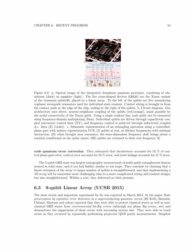
CHAPTER 6. RECENT PROGRESS 54
Figure 6.2: a, Optical image of the integrated Josephson quantum processor, consisting of alu-minium (dark) on sapphire (light). The five cross-shaped devices (Q0Q4) are the Xmon variantof the transmon qubits30, placed in a linear array. To the left of the qubits are five meanderingcoplanar waveguide resonators used for individual state readout. Control wiring is brought in fromthe contact pads at the edge of the chip, ending at the right of the qubits. b, Circuit diagram. Ourarchitecture uses direct, nearest-neighbour coupling of the qubits (red/orange), made possible bythe nodal connectivity of the Xmon qubit. Using a single readout line, each qubit can be measuredusing frequency-domain multiplexing (blue). Individual qubits are driven through capacitively cou-pled microwave control lines (XY), and frequency control is achieved through inductively coupledd.c. lines (Z) (violet). c, Schematic representation of an entangling operation using a controlled-phase gate with unitary representation UCZ; (I) qubits at rest, at distinct frequencies with minimalinteraction; (II) when brought near resonance, the state-dependent frequency shift brings about arotation conditional on the qubit states; (III) qubits are returned to their rest frequency [8]
.
code quantum error correction. They estimated that decoherence accounts for 55 % of con-trol phase gate error, control error accounts for 24 % error, and state leakage accounts for 21 % error.
The 5-qubit GHZ state was largest tomographic measurement of multi-qubit entanglement demon-strated in solid state, and it too had fidelity similar to ion traps. They conclude by claiming that alinear extension of the array to larger number of qubits is straightforward, and that implementing a2D array will be somewhat more challenging (due to a more complicated wiring and readout design)but also straightforward. Within a year, they delivered on their promise.
6.3 9-qubit Linear Array (UCSB 2015)
The most recent and important experiment by far was reported in March 2015. In the paper Statepreservation by repetitive error detection in a superconducting quantum circuit [29] Kelly, Barends,Cleland, Martinis and others reported that they were able to protect classical states as well as non-classical GHZ states from environmental bit-flip errors (although not phase flip errors...yet) anddemonstrate the suppression of those errors with increasing system size. They were able to trackerrors as they occurred by repeatedly performing projective QND parity measurements. Simplest
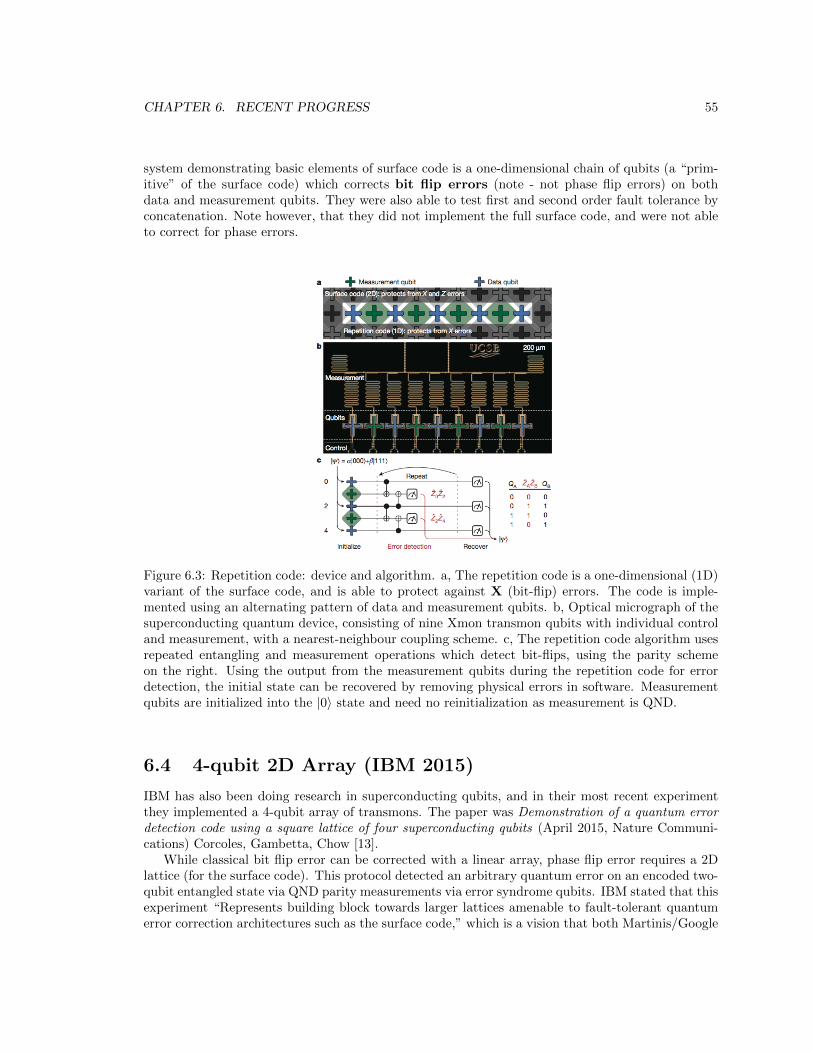
CHAPTER 6. RECENT PROGRESS 55
system demonstrating basic elements of surface code is a one-dimensional chain of qubits (a “prim-itive” of the surface code) which corrects bit flip errors (note - not phase flip errors) on bothdata and measurement qubits. They were also able to test first and second order fault tolerance byconcatenation. Note however, that they did not implement the full surface code, and were not ableto correct for phase errors.
Figure 6.3: Repetition code: device and algorithm. a, The repetition code is a one-dimensional (1D)variant of the surface code, and is able to protect against X (bit-flip) errors. The code is imple-mented using an alternating pattern of data and measurement qubits. b, Optical micrograph of thesuperconducting quantum device, consisting of nine Xmon transmon qubits with individual controland measurement, with a nearest-neighbour coupling scheme. c, The repetition code algorithm usesrepeated entangling and measurement operations which detect bit-flips, using the parity schemeon the right. Using the output from the measurement qubits during the repetition code for errordetection, the initial state can be recovered by removing physical errors in software. Measurementqubits are initialized into the |0〉 state and need no reinitialization as measurement is QND.
6.4 4-qubit 2D Array (IBM 2015)
IBM has also been doing research in superconducting qubits, and in their most recent experimentthey implemented a 4-qubit array of transmons. The paper was Demonstration of a quantum errordetection code using a square lattice of four superconducting qubits (April 2015, Nature Communi-cations) Corcoles, Gambetta, Chow [13].
While classical bit flip error can be corrected with a linear array, phase flip error requires a 2Dlattice (for the surface code). This protocol detected an arbitrary quantum error on an encoded two-qubit entangled state via QND parity measurements via error syndrome qubits. IBM stated that thisexperiment “Represents building block towards larger lattices amenable to fault-tolerant quantumerror correction architectures such as the surface code,” which is a vision that both Martinis/Google
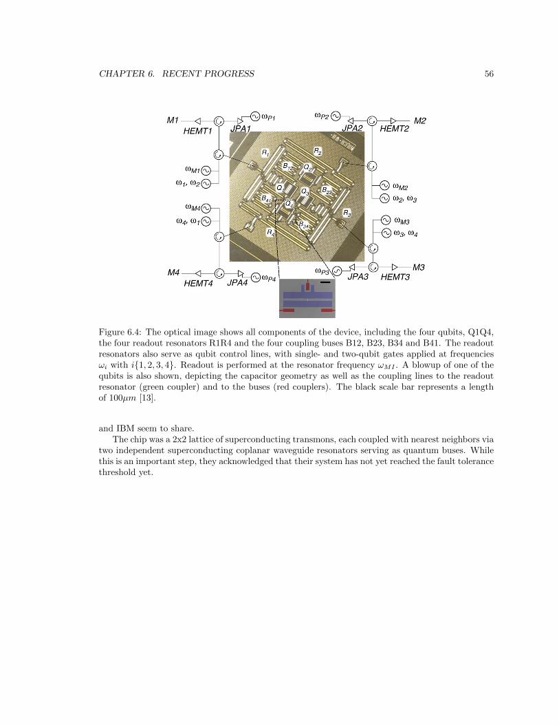
CHAPTER 6. RECENT PROGRESS 56
Figure 6.4: The optical image shows all components of the device, including the four qubits, Q1Q4,the four readout resonators R1R4 and the four coupling buses B12, B23, B34 and B41. The readoutresonators also serve as qubit control lines, with single- and two-qubit gates applied at frequenciesωi with i1, 2, 3, 4. Readout is performed at the resonator frequency ωMI . A blowup of one of thequbits is also shown, depicting the capacitor geometry as well as the coupling lines to the readoutresonator (green coupler) and to the buses (red couplers). The black scale bar represents a lengthof 100µm [13].
and IBM seem to share.The chip was a 2x2 lattice of superconducting transmons, each coupled with nearest neighbors via
two independent superconducting coplanar waveguide resonators serving as quantum buses. Whilethis is an important step, they acknowledged that their system has not yet reached the fault tolerancethreshold yet.
CHAPTER 6. RECENT PROGRESS 57
6.5 Conclusion
We carefully developed of the quantum circuit formalism of quantum computing, starting with twolevel quantum systems and the Pauli spin matrices and building up to the celebrated algorithmsof Shor and Grover. The limitations of these algorithms were also discussed. These theoreticaldevelopments addressed some of the original questions posed by Feynman - among other things,they established that a computer built from quantum components is, indeed, fundamentally differentfrom a classical computer.
We then developed the problem of quantum error correction, which stems from the fundamentalphysics of quantum systems but can be abstracted to a set of five possible transformations. Thetwo most important of these are energy relaxation, where the qubit loses energy to the environmentand relaxes from the |1〉 state to the |0〉 state, and dephasing, which changes the relative phase ofa qubit in a superposition. Novel error correction schemes had to be formulated in order to correctfor these possible errors, as classical error correction schemes cannot be implemented on qubits dueto the no cloning theorem. We also briefly touched on the threshold theorems, and the possibilityof efficient quantum computing given a probability of error below a threshold for a particular errorcorrection scheme. The surface code has the highest (and therefore most approachable) thresholdof the error correction codes, which is why it is considered an important benchmark. Although thisbenchmark has not been fully reached, the necessary coherence time for a single qubit in the surfacecode has been reached.
Next we explained the framework surrounding the physical implementation of superconductingqubits, highlighting the unique properties of the Josephson junction and the similarity of Josephsoncircuits with classical LC/RLC circuits. In particular, we show that the frequency and phase of thedriving voltage allow for elegant manipulation of the Pauli spin matrices.
Finally, we investigated the phenomenon of decoherence more closely to understand how inter-action with the environment influences a particular quantum system. We introduced the canonicalspin-boson and spin-spin models, and discussed them in the context of superconducting qubits. Inthis discussion we explained how coherence could be improved both by clever circuit design and bybetter fabrication techniques. This also explains the five-fold increase in coherence times since 2000.We finished off the subject with some recent examples of superconducting qubit research.
Martinis and his group at UCSB built qubits above the surface code threshold but have not yetbuilt a 2D array in order to correct both bit and phase flip errors. IBM has build a 2D array, butits qubits are below surface code threshold. It seems that:
1. Coherence times are improving and don’t seem to have reached a ceiling
2. Arrays of qubits are extremely well controlled, and do not seem to change behavior when scaledup
3. Large scale industrial manufacturing of superconducting qubits will not be difficult given cur-rent fabrication techniques
In the face of all the theoretical results and experimental progress, it is not so hard to believe thatcoherence in superconducting qubits might improve just a bit more - at least just enough to makefault tolerant circuits and fault tolerant computing a reality.

Bibliography
[1] Google partners with ucsb to build quantum processors forartificial intelligence. http://techcrunch.com/2014/09/02/
google-partners-with-ucsb-to-build-quantum-processors-for-artificial-intelligence/.Accessed: 2015-09-16.
[2] Hardware initiative at quantum artificial intelligence lab. http://googleresearch.blogspot.com/2014/09/ucsb-partners-with-google-on-hardware.html. Accessed: 2015-09-16.
[3] The man who will build googles elusive quantum computer. http://www.wired.com/2014/09/martinis/. Accessed: 2015-09-16.
[4] “shtetl optimized: Shor i’ll do it’. http://www.scottaaronson.com/blog/?p=208. Accessed:2015-010-18.
[5] David Z Albert and David Z Albert. Quantum mechanics and experience. Harvard UniversityPress, 2009.
[6] Adriano Barenco, Charles H Bennett, Richard Cleve, David P DiVincenzo, Norman Margolus,Peter Shor, Tycho Sleator, John A Smolin, and Harald Weinfurter. Elementary gates forquantum computation. Physical Review A, 52(5):3457, 1995.
[7] R Barends, J Kelly, A Megrant, D Sank, E Jeffrey, Y Chen, Y Yin, B Chiaro, J Mutus, C Neill,et al. Coherent josephson qubit suitable for scalable quantum integrated circuits. Physicalreview letters, 111(8):080502, 2013.
[8] R Barends, J Kelly, A Megrant, A Veitia, D Sank, E Jeffrey, TC White, J Mutus, AG Fowler,B Campbell, et al. Superconducting quantum circuits at the surface code threshold for faulttolerance. Nature, 508(7497):500–503, 2014.
[9] John Stewart Bell. Speakable and unspeakable in quantum mechanics: Collected papers onquantum philosophy. Cambridge university press, 2004.
[10] Yu Chen, C Neill, P Roushan, N Leung, M Fang, R Barends, J Kelly, B Campbell, Z Chen,B Chiaro, et al. Qubit architecture with high coherence and fast tunable coupling. Physicalreview letters, 113(22):220502, 2014.
[11] John Clarke and Frank K Wilhelm. Superconducting quantum bits. Nature, 453(7198):1031–1042, 2008.
[12] Richard Cleve, Artur Ekert, Chiara Macchiavello, and Michele Mosca. Quantum algorithmsrevisited. In Proceedings of the Royal Society of London A: Mathematical, Physical and Engi-neering Sciences, volume 454, pages 339–354. The Royal Society, 1998.
58
BIBLIOGRAPHY 59
[13] AD Corcoles, Easwar Magesan, Srikanth J Srinivasan, Andrew W Cross, M Steffen, Jay MGambetta, and Jerry M Chow. Demonstration of a quantum error detection code using asquare lattice of four superconducting qubits. Nature communications, 6, 2015.
[14] FM Cucchietti, Juan Pablo Paz, and WH Zurek. Decoherence from spin environments. PhysicalReview A, 72(5):052113, 2005.
[15] David Deutsch. Quantum theory, the church-turing principle and the universal quantum com-puter. In Proceedings of the Royal Society of London A: Mathematical, Physical and EngineeringSciences, volume 400, pages 97–117. The Royal Society, 1985.
[16] Michel Devoret, Benjamin Huard, Robert Schoelkopf, and Leticia F Cugliandolo. QuantumMachines: Measurement and Control of Engineered Quantum Systems, volume 96. OxfordUniversity Press, 2014.
[17] Michel H Devoret, A Wallraff, and JM Martinis. Superconducting qubits: A short review. arXivpreprint cond-mat/0411174, 2004.
[18] Albert Einstein, Boris Podolsky, and Nathan Rosen. Can quantum-mechanical description ofphysical reality be considered complete? Physical review, 47(10):777, 1935.
[19] Richard P Feynman. Simulating physics with computers. International journal of theoreticalphysics, 21(6/7):467–488, 1982.
[20] Richard Phillips Feynman and Frank Lee Vernon. The theory of a general quantum systeminteracting with a linear dissipative system. Annals of physics, 24:118–173, 1963.
[21] Austin G Fowler, Matteo Mariantoni, John M Martinis, and Andrew N Cleland. Surface codes:Towards practical large-scale quantum computation. Physical Review A, 86(3):032324, 2012.
[22] Edward Fredkin and Tommaso Toffoli. Conservative logic. Springer, 2002.
[23] Daniel M Greenberger, Michael A Horne, and Anton Zeilinger. Going beyond bells theorem. InBells theorem, quantum theory and conceptions of the universe, pages 69–72. Springer, 1989.
[24] David J Griffiths. Introduction to quantum mechanics, 1995.
[25] Lov K Grover. A fast quantum mechanical algorithm for database search. In Proceedings of thetwenty-eighth annual ACM symposium on Theory of computing, pages 212–219. ACM, 1996.
[26] Eric Joos and H Dieter Zeh. The emergence of classical properties through interaction with theenvironment. Zeitschrift fur Physik B Condensed Matter, 59(2):223–243, 1985.
[27] Erich Joos, H Dieter Zeh, Claus Kiefer, Domenico JW Giulini, Joachim Kupsch, and Ion-Olimpiu Stamatescu. Decoherence and the appearance of a classical world in quantum theory.Springer Science & Business Media, 2013.
[28] Brian David Josephson. Possible new effects in superconductive tunnelling. Physics letters,1(7):251–253, 1962.
[29] J Kelly, R Barends, AG Fowler, A Megrant, E Jeffrey, TC White, D Sank, JY Mutus, B Camp-bell, Yu Chen, et al. State preservation by repetitive error detection in a superconductingquantum circuit. Nature, 519(7541):66–69, 2015.
BIBLIOGRAPHY 60
[30] Thaddeus D Ladd, Fedor Jelezko, Raymond Laflamme, Yasunobu Nakamura, Christopher Mon-roe, and Jeremy L OBrien. Quantum computers. Nature, 464(7285):45–53, 2010.
[31] Dan C Marinescu and Gabriela M Marinescu. Approaching quantum computing. Prentice Hall,2005.
[32] John M Martinis and A Megrant. Ucsb final report for the csq program: Review of decoherenceand materials physics for superconducting qubits. arXiv preprint arXiv:1410.5793, 2014.
[33] Robert McDermott. Materials origins of decoherence in superconducting qubits. Applied Su-perconductivity, IEEE Transactions on, 19(1):2–13, 2009.
[34] Michael A Nielsen and Isaac L Chuang. Quantum computation and quantum information.Cambridge university press, 2010.
[35] William D Oliver and Paul B Welander. Materials in superconducting quantum bits. MRSbulletin, 38(10):816–825, 2013.
[36] Roland Omnes. The interpretation of quantum mechanics. Princeton University Press, 1994.
[37] Maximilian A Schlosshauer. Decoherence: and the quantum-to-classical transition. SpringerScience & Business Media, 2007.
[38] Alexander Shnirman, Yuriy Makhlin, and Gerd Schon. Noise and decoherence in quantumtwo-level systems. Physica Scripta, 2002(T102):147, 2002.
[39] Peter W Shor. Algorithms for quantum computation: Discrete logarithms and factoring. InFoundations of Computer Science, 1994 Proceedings., 35th Annual Symposium on, pages 124–134. IEEE, 1994.
[40] Tommaso Toffoli. Reversible computing. Springer, 1980.
[41] David Wallace. The emergent multiverse: Quantum theory according to the Everett interpreta-tion. Oxford University Press, 2012.
[42] William K Wootters and Wojciech H Zurek. A single quantum cannot be cloned. Nature,299(5886):802–803, 1982.
[43] Wojciech H Zurek. Environment-induced superselection rules. Physical Review D, 26(8):1862,1982.
Appendix A
Recent UCSB Publications
Just to get a sense of the fast pace research coming out of the UCSB (now Google) group, here is a listof their most recent publications and submitted papers from the group website web.physics.ucsb.edu/martinisgroup/publications.shtml[accessed October 7, 2015]. The following are from 2015 alone:
• Qubit metrology for building a fault-tolerant quantum computer John M. MartinisAccepted for publication in NPJ Quantum Information (2015).
• Measuring and Suppressing Quantum State Leakage in a Superconducting QubitZijun Chen, Julian Kelly, Chris Quintana, R. Barends, B. Campbell, Yu Chen, B. Chiaro, A.Dunsworth, A. G. Fowler, E. Lucero, E. Jeffrey, A. Megrant, J. Mutus, M. Neeley, C. Neill, P.J. J. O’Malley, P. Roushan, D. Sank, A. Vainsencher, J. Wenner, T. C. White, A. N. Korotkov,John M. Martinis Submitted (2015). arXiv:1509.05470
• Violating the Bell-Leggett-Garg inequality with weak measurement of an entan-gled state T.C. White, J.Y. Mutus, J. Dressel, J. Kelly, R. Barends, E. Jeffrey, D. Sank,A. Megrant, B. Campbell, Yu Chen, Z. Chen, B. Chiaro, A. Dunsworth, I.-C. Hoi, C. Neill,P.J.J. O’Malley, P. Roushan, A. Vainsencher, J. Wenner, A. N. Korotkov, John M. MartinisSubmitted (2015). arXiv:1504.02707
• Scalable extraction of error models from the output of error detection circuitsAustin G. Fowler, D. Sank, J. Kelly, R. Barends, John M. Martinis Submitted (2014). arXiv:1405.1454
• Quantum theory of a bandpass Purcell filter for qubit readout Eyob A. Sete, JohnM. Martinis, Alexander N. Korotkov PRA 92, 012325 (2015). arXiv:1504.06030
• Tunable coupler for superconducting Xmon qubits: Perturbative nonlinear modelMichael R. Geller, Emmanuel Donate, Yu Chen, Michael T. Fang, Nelson Leung, Charles Neill,Pedram Roushan, John M. Martinis PRA 92, 012320 (2015). arXiv:1405.1915
• Digital quantum simulation of fermionic models with a superconducting circuitR. Barends, L. Lamata, J. Kelly, L. Garca-lvarez, A. G. Fowler, A. Megrant, E. Jeffrey, T.C. White, D. Sank, J. Y. Mutus, B. Campbell, Yu Chen, Z. Chen, B. Chiaro, A. Dunsworth,I.-C. Hoi, C. Neill, P. J. J. O’Malley, C. Quintana, P. Roushan, A. Vainsencher, J. Wenner, E.Solano, John M. Martinis Nature Communications 6, 7654 (2015). arXiv:1501.07703
• Traveling wave parametric amplifier with Josephson junctions using minimal res-onator phase matching T.C. White, J.Y. Mutus, I.-C. Hoi, R. Barends, B. Campbell, Yu
61
APPENDIX A. RECENT UCSB PUBLICATIONS 62
Chen, Z. Chen, B. Chiaro, A. Dunsworth, E. Jeffrey, J. Kelly, A. Megrant, C. Neill, P.J.J.O’Malley, P. Roushan, D. Sank, A. Vainsencher, J. Wenner, S. Chaudhuri, J. Gao, John M.Martinis APL 106, 242601 (2015). arXiv:1503.04364
• Universal quantum simulation with prethreshold superconducting qubits: Single-excitation subspace method Michael R. Geller, John M. Martinis, Andrew T. Sornborger,Phillip C. Stancil, Emily J. Pritchett, Hao You, Andrei Galiautdinov PRA 91, 062309 (2015).arXiv:1505.04990
• Qubit metrology of ultralow phase noise using randomized benchmarking P. J. J.O’Malley, J. Kelly, R. Barends, B. Campbell, Y. Chen, Z. Chen, B. Chiaro, A. Dunsworth,A. G. Fowler, I.-C. Hoi, E. Jeffrey, A. Megrant, J. Mutus, C. Neill, C. Quintana, P. Roushan,D. Sank, A. Vainsencher, J. Wenner, T. C. White, A. N. Korotkov, A. N. Cleland, John M.Martinis Phys. Rev. Applied 3, 044009 (2015). arXiv:1411.2613
Appendix B
Recent Yale Publications
The following is a list of the Devoret group’s most recent publications and submitted papers fromthe group website qulab.eng.yale.edu/publications page.html [accessed November 4, 2015]. Thefollowing are from 2015:
• Remote Entanglement by Coherent Multiplication of Concurrent Quantum SignalsA. Roy, L. Jiang, A. D. Stone, M. H. Devoret Phys. Rev. Lett. 115, 150503 (2015)
• 2.5D circuit quantum electrodynamics Z. K. Minev, K. Serniak, I.M. Pop, Z. Leghtas,K. Sliwa, M. Hatridge, L. Frunzio, R. J. Schoelkopf, M. H. Devoret arXiv:1509.01619v1
• Surface Participation and Dielectric Loss in Superconducting Qubits C. Wang, C.Axline, Y. Gao, T. Brecht, L. Frunzio, M. H. Devoret, R. J. Schoelkopf arXiv:1509.01854v1
• Multilayer Microwave Integrated Quantum Circuits for Scalable Quantum Com-puting T. Brecht, W. Pfaff, C. Wang, Y. Chu, L. Frunzio, M. H. Devoret, R. J. SchoelkopfarXiv:1509.01127v1
• Demonstration of Micromachined Superconducting Cavities T. Brecht, M. Reagor,Y. Chu, W. Pfaff, C. Wang, L. Frunzio, M. H. Devoret, R. J. Schoelkopf arXiv:1509.01119v1
• Comparing and combining measurement-based and driven-dissipative entangle-ment stabilization Y. Liu, S. Shankar, N. Ofek, M. Hatridge, A. Narla, K. M. Sliwa, L.Frunzio, R. J. Schoelkopf, M. H. Devoret arXiv:1509.00860v1
• A Quantum Memory with Near-millisecond Coherence in Circuit QED M. Reagor,W. Pfaff, C. Axline, R. W. Heeres, N. Ofek, K. Sliwa, E. Holland, C. Wang, J. Blumoff, K.Chou, M. Hatridge, L. Frunzio, M. H. Devoret, L. Jiang, R. J. Schoelkopf arXiv:1508.05882v2
• Characterizing Entanglement of An Artificial Atom and a Cavity Cat State withBell’s Inequality B. Vlastakis, A. Petrenko, N. Ofek, L. Sun, Z. Leghtas, K. Sliwa, M.Hatridge, J. Blumoff, L. Frunzio, M. Mirrahimi, L. Jiang, M. H. Devoret, and R. J. SchoelkopfarXiv:1504.02512v1
• Single-Photon Resolved Cross-Kerr Interaction for Autonomous Stabilization ofPhoton-number States E. T. Holland, B. Vlastakis, R. W. Heeres, M. J. Reagor, U.Vool, Z. Leghtas, L. Frunzio, G. Kirchmair, M. H. Devoret, M. Mirrahimi, R. J. SchoelkopfarXiv:1504.03382v1
63
APPENDIX B. RECENT YALE PUBLICATIONS 64
• Cavity State Manipulation Using Photon-Number Selective Phase Gates R. W.Heeres, B. Vlastakis, E. Holland, S. Krastanov, V. Albert, L. Frunzio, L. Jiang, R. J. SchoelkopfarXiv:1503.01496v1

APPENDIX B. RECENT YALE PUBLICATIONS 65
Figure B.1: Thesis on a napkin
Related Documents