Decision by sampling: The role of the decision environment in risky choice

Decision by Sampling: The Role of the Decision Environment inRiskyChoice

Neil StewartUniversity of Warwick

Decision by sampling (DbS) is a theory about how our environment shapes the decisions thatwe make. Here, I review the application of DbS to risky decision making. According to clas-sical theories of risky decision making, people make stable transformations between outcomesand probabilities and their subjective counterparts using fixed psychoeconomic functions. DbSoffers a quite different account. In DbS, the subjective value of an outcome or probability isderived from a series of binary, ordinal comparisons with a sample ofother outcomes or prob-abilities from the decision environment. In this way, the distribution of attribute values in theenvironment determines the subjective valuations of outcomes and probabilities. I show howDbS interacts with the real-world distributions of gains, losses, and probabilities to produce theclassical psychoeconomic functions. I extend DbS to account for preferences in benchmarkdata sets. Finally, in a challenge to the classical notion of stable subjective valuations, I reviewevidence that manipulating the distribution of attribute values in the environment changes oursubjective valuations just as DbS predicts.

Risky decision making is a central part of human cogni-tion. One often has to choose between alternative actionswhere the outcomes associated with each action are uncer-tain. Because our environment is not a deterministic place,most everyday decisions involve some element of risk. Andmany of our most important decisions also involve risk. Forexample, financial decisions involving saving and borrowingare risky because of variability in interest rates and the stockmarket. Medical decisions are risky because the effective-ness of treatments will vary from case to case.

In this review, I show how the risky decisions that wemake are influenced by the statistical distributions of risksand rewards in the environment. Our sensitivity to the dis-tribution of attributes within the environment emerges fromour use of a set of domain-general cognitive tools to makerisky decisions and is captured in the decision by samplingmodel (DbS, Stewart, Chater, & Brown, 2006). I begin by re-viewing what might be considered to be the most prominenttheory of risky decision making: prospect theory (Kahneman& Tversky, 1979; Tversky & Kahneman, 1992). Prospecttheory provides an excellent description of human risky de-

Neil Stewart, Department of Psychology, University of Warwick,Coventry, CV4 7AL, UK. Email: [email protected] thank the EPS for their invitation to write this article. The articlefollows the EPS Prize Lecture delivered at UCL in January 2008.I would like to thank all of my collaborators, but must especiallythank Gordon D. A. Brown and Nick Chater to whom I am greatlyindebted. Thanks also to Nigel Harvey and an anonymous reviewer.This research was supported by ESRC grant RES-062-23-0952.Stewart, N. (2009). Decision by sampling: The role of the deci-sion environment in risky choice.Quarterly Journal of ExperimentPsychology, 62,1041-1062.

cision making. In the second part of the article, I show howit is possible to derive the prospect-theory description fromthe real-world distribution of risks and rewards under the as-sumptions of the DbS model. In the penultimate part of thisarticle, I show how the DbS model has been successfully de-veloped to provide a process account of the risky decisionsthat we make. Finally, in a direct test of the DbS model, Ireview new experimental evidence for the link between thedistribution of attribute values in the environment and therisky decisions that we make.

Descriptive Models of RiskyDecision Making

If you were offered a choice between either (a) £1,000 or(b) a 50% chance of £2,000 otherwise £0 which would youchoose? Questions like these have been used extensively inthe study of human risky decision making as carefully con-trolled proxies for real-life risky decisions. Lopes and Oden(1983), and later Kahneman (Kahneman & Tversky, 2000),make the analogy between the study of choices between sim-ple gambles in risky decision making and the study of thefruit fly in genetics. Returning to the example, the majorityof people are risk averse and have a preference for the cer-tain £1,000. This result is immediately useful in ruling outperhaps the most obvious candidate—expected value—as amodel for human risky decision making.

In expected value theory, people prefer the option whichoffers them the highest average payoff. For the first option,the expected value is £1,000. For the second option, the ex-pected values is also£1,000= 1/2×£2,000+1/2×£0. Thetwo options have the same expected value and so expectedvalue does not capture the preference for the first option.

Economists have a theory that does capture this risk-averse preference: expected utility (EU) theory (Bernoulli,

2 STEWART

0 500 1000 1500 2000 2500

Util

ity

Money / £

Figure 1. A power law utility functionU(x) = xα transformsmoneyx into its subjective equivalentU(x).

1738/1954; see von Neumann & Morgenstern, 1947 for anaxiomatisation). In EU theory, money is transformed intoutility before expectations are taken. Figure 1 shows a typicalpower-law utility function whereU(x) = xα. (Bernoulli sug-gested a logarithmic function, but credits Cramer, 1728, withsuggesting the square root function. For investigations intofunctional forms for utility functions, see Bell & Fishburn,1999; Daniels & Keller, 1992; Fishburn & Kochenberger,1979.) The utility function has a concave-downward shape(whenα < 1 the function is curved downwards) and this al-lows the model to capture the risk aversion displayed in thepreference for the certain £1,000. Specifically, because theutility of £1,000 is more than half the utility of £2,000 whenthe utility curve is concave, EU theory predicts a higher util-ity for, and thus a preference for, the first option. Specifically,U(£1,000) > 1/2×U(£2,000)+ 1/2×U(£0) whenα < 1.

The concave shape of the utility function captures and ex-plains risk aversion. But there is evidence that utility func-tions have this concave-downward form when they are mea-sured in risk free scenarios. For example, Galanter (1962)found a concave shape by asking participants to judge howmuch money would make them twice as happy as a refer-ence amount. Other theories place risk aversion elsewhere(see Davies & Satchell, 2007, for a recent discussion).

EU theory plays a foundational role in economics, be-cause it is used as a model of the rational individual inmany models of the economy. Its mathematical simplicityhas given it great appeal. Unfortunately, although it capturesrisk aversion, it is not a complete description of human riskydecision making. There are many examples of preferencepatterns that violate EU theory (for reviews see Allais, 1953;Birnbaum, 2008; Camerer, 1995; Luce, 2000; Schoemaker,1982; Starmer, 2000). Committing a grave injustice to thevolume of empirical work demonstrating violations of EUtheory, I will present here only two examples taken fromKahneman and Tversky (1979). First, consider the pair ofchoices in Table 1. These choices are an example of thecommon-ratio effect (Allais, 1953). Choice 1 offers either

(a) an 80% chance of £4,000 otherwise £0 or (b) £3,000.80% of Kahneman and Tversky’s participants preferred thesure £3,000. Choice 2 offers either (a) a 20% chance of£4000 otherwise £0 or (b) a 25% chance of £3,000 otherwisenothing. Now the majority of participants preferred the 20%chance of £4,000.

The preference for Prospect B in Choice 1 but ProspectA in Choice 2 represents a violation of EU theory be-cause Choice 2 is generated from Choice 1 by multiplyingprobabilities by 1/4. Because the same thing was done toboth prospects in the choice, preference should not switchfrom one side to the other. More specifically, the prefer-ence for Prospect B in Choice 1 implies.80×U(£4,000) <1.00×U(£3,000) but the preference for Prospect A in Choice2 implies.20×U(£4,000) > .25×U(£3,000). These two in-equalities contradict one another and cannot both be true, andthus this pattern of preference violates EU theory. Althoughthis violation is demonstrated at the population level, a largeproportion of individual participants show the preferenceforProspect B in Choice 1 and Prospect A in Choice 2 whentested with both choices (e.g., Carlin, 1992).

Kahneman and Tversky (1979) developed prospect theoryto account for violations like the common-ratio effect. Theydeliberately kept their formulation close to EU theory, andin-corporated the minimum modifications necessary to accountfor the data. The first key difference is the inclusion of aprobability-weighting function. The left panel of Figure 2shows the decision weighting function from Tversky andKahneman’s (1992) cumulative prospect theory. Just as realworld outcomes are transformed into their subjective utilityequivalents by the utility function, Kahneman and Tverskysuggested that objective probabilities are transformed intosubjective probabilities. The probability-weighting functionis most sensitive (i.e., steepest) near 0 and 1 and is least sen-sitive (i.e., flattest) for mid-range probabilities.1

The probability-weighting function allows prospect the-ory to account for the common-ratio effect. Specifically, thedifference between the weights of the .8 and 1.0 probabili-ties in Choice 1 is large, because the probability-weightingfunction is most sensitive in this region. But the differencebetween the weights of the .2 and .25 probabilities in Choice2 is small, because the probability-weighting function is lesssensitive in this region. Thus although the ratio of the ob-jective probabilities is the same in Choices 1 and 2, the ratioof the weights is not. As a result, relatively more weight isplaced on the £3,000 in Choice 1 but relatively more weightis placed on the £4,000 in Choice 2. The reversal in pref-erence between the two choices results from the shift in therelative sizes of the decision weights.

1 In fact, Kahneman and Tversky maintained a difference be-tween subjective probability and decision weighting. A subjectiveprobability is the psychophysical transform of the objective proba-bility. A decision weight is the emphasis given to the correspond-ing outcome. So one might have an accurately calibrated subjectiveprobability for an objectively unlikely event (e.g., knowing winningthe lottery is very unlikely), but still behave as if the event is morelikely than it really is because one weights the associated outcometoo heavily (e.g., by buying a ticket).

DECISION BY SAMPLING 3

Table 1The Common-Ratio Effect

Prospect A Prospect BChoice Amount Probability % chosen Amount Probability % chosen

1 £4,000 .8 20% £3,000 1.0 80%£0 .2

2 £4,000 .2 65% £3,000 .25 35%£0 .8 £0 .75

0

1

0 1

Wei

ght

Probability

Probability Weighting Function

0

0

Val

ue

Amount

Value Function

Figure 2. A: Example probability-weighting function (top) andvalue function (bottom) from cumulative prospect theory.

A second violation of EU theory is shown in Table 2.Choice 1 pays participants an initial payment of £1,000. Par-ticipants are then offered (a) a 50% chance of winning an-other £1,000 otherwise £0 or (b) £500. 84% of participantsprefer Prospect B. Choice 2 pays participants an initial pay-ment of £2,000. Participants are then offered (a) a 50%chance of losing £1,000 or otherwise losing nothing or (b)a sure loss of £500. 69% of participants prefer Prospect A.

The preference for Prospect B in Choice 1 but ProspectA in Choice 2 represents a violation of EU theory becauseChoices 1 and 2 lead to the same net outcomes. For bothchoices, when initial endowments are integrated with theprospect payoffs, Prospect A offers a 50% chance of £1,000and a 50% chance of £2,000 and Prospect B offers £1,500for sure. Kahneman and Tversky (1979) refer to this effectas a framing effect, because whether outcomes were framedas gains or losses switched people’s preferences from riskaverse to risk prone.

Kahneman and Tversky (1979) incorporated this findinginto prospect theory by again making a small change to theEU framework. The right panel in Figure 2 shows a re-vised function for transforming amounts into their subjec-tive equivalents. In prospect theory, this function is calledthe value function (cf. the utility function in EU theory). Inthe top-right quadrant, the function is concave, just like theutility function from EU theory, to capture risk-averse be-haviour in the domain of gains. In the bottom-left quadrant,the function is convex to capture risk seeking behaviour inthe domain of losses. The function is also steeper for lossesthan for gains to capture the fact that people do not like toplay zero expected value gambles involving gains and losses(but see Ert & Erev, 2007). For example, most people do

not want to play a gamble that offers equal chances to gain£1,000 and to lose £1,000.

Prospect theory provides a good description of the riskydecisions that people make. The shapes of the probability-weighting function and the value function are chosen to pro-vide this good description. In addition to prospect theory,there are many other theories that have been derived from EUtheory including subjective EU theory (Edwards, 1962; Sav-age, 1954), regret theory (Loomes & Sugden, 1982), rank-dependent utility theory (Quiggin, 1993), decision field the-ory (Busemeyer & Townsend, 1993), and the transfer-of-attention-exchange model (Birnbaum & Chavez, 1997; Birn-baum, 2008). What each of these theories has in commonis the assumption that outcomes and probabilities are trans-formed into their subjective equivalents and expectationsaretaken. The different theories assume different transformsofamounts and probabilities, and these different transformsal-low the models to describe the decision people make. In theremainder of this article I want to consider DbS. Accordingto DbS, psychoeconomic functions have no psychologicalstatus (i.e., we do not have look-up functions inside our headsfor converting between money and utility or probability andsubjective probability). Instead, psychoeconomic functionsare revealed from choice data: they describe the choices peo-ple make, but not the psychology of choosing.

How the Distribution of AttributeValues Shapes Revealed

Psychoeconomic Functions

DbS assumes that three simple cognitive tools are the ba-sis for decision making: binary, ordinal comparison; sam-pling; and frequency accumulation. Stewart et al. (2006)review the evidence for the ubiquity of these domain-generalcognitive tools. Very briefly, the binary, ordinal comparisontool is motivated by findings in psychophysics, where peopleare rather good at saying which stimulus in a pair is the largerstimulus, but are rather bad at estimating the magnitudes ofindividual stimuli (Laming, 1997; Stewart, Brown, & Chater,2005). The sampling tool is motivated by the judgement anddecision making literature, where hypotheses (in norm the-ory, Kahneman & Miller, 1986) or uncertainties (in supporttheory, Tversky & Koehler, 1994) are compared to a smallsample of exemplars from memory. More generally, that ourworking memories can hold a small sample of informationfrom the immediate context and from long-term memory iswell established. The frequency accumulation tool is moti-vated by the finding that we are rather good at keeping track

4 STEWART

Table 2The Framing Effect

Prospect A Prospect BChoice Amount Probability % chosen Amount Probability % chosen

1 Given £1,000 initially£1,000 .5 16% £500 1.0 84%

£0 .52 Given £2,000 initially

-£1,000 .5 69% -£500 1.0 31%£0 .5

of and manipulating frequencies (e.g., Gigerenzer & Hof-frage, 1995; Sedlmeier & Betsch, 2002).

In DbS these three cognitive tools are used to derive thesubjective value of an attribute value (i.e., to derive the psy-chological significance of a probability or of an outcome).Specifically, the subjective value is constructed from a se-ries of binary, ordinal comparisons within a set of attributevalues sampled both from the immediate context of the deci-sion and from long-term memory. For each attribute value, afrequency count is kept of the number of favourable compar-isons. The subjective value of an attribute is given by the pro-portion of favourable comparisons. For example, considerhow the subjective value of a gain of £12 might be arrived at.The gain is compared to a small sample in working memory,say £1, £5, £33, £45, and £82. The sample will come fromboth the other attribute values in the immediate context andfrom previous experiences stored in long-term memory. Aseries of binary, ordinal comparisons are made between thetarget attribute of £12 and the attributes in the sample. Of thefive possible comparisons, two of them are favourable (com-parisons to £1 and £5). Thus the probability of a favourablecomparison is 2/5, and in DbS this probability is used as thesubjective value.

Of course, the subject value is completely dependent uponthe distribution of attribute values in memory. Stewart et al.(2006) made the assumption that the distribution of attributevalues in long-term memory reflects the real-world distribu-tion (cf. J. R. Anderson & Schooler, 1991). Stewart et al.showed how the value and probability-weighting functionsseen in prospect theory can be derived from the distributionsof probabilities and amounts encountered in the environment,and thus provided an independent motivation for the particu-lar shapes of these psychoeconomic functions.

The top panel of Figure 3 shows the credits into currentaccounts held by a large UK bank. The distribution is usedas a crude approximation to the distribution of gains peopleencounter in the world. The figure is aggregated across manycurrent accounts and represents about 320,000 payments intotal. There are two key properties of this distribution. First,the distribution is very roughly power-law (i.e., is roughlylinear on the log-log plot). Thus, although one might ques-tion whether the distribution of credits into UK current ac-counts is truly representative of the distribution of gainsin anindividual person’s long-term memory, there is good reasonto expect the long-term memory distribution to have similar

1

10

100

1000

10000

100000

1 10 100 1000 10000 100000

Fre

quen

cy

Credit/£

Credits

1

10

100

1000

10000

100000

1 10 100 1000 10000 100000

Fre

quen

cy

Debit/£

Debits

Figure 3. The frequency of credits to (top) and debits from (bot-tom) a large sample of UK current accounts. Adapted from Stewart,Chater, and Brown (2006).

properties. Power law distributions are very common (Bak,1997) and describe the distributions of prices of many ev-eryday items (e.g., Stewart et al., 2006; Stewart & Simpson,2008). Second, and more importantly for the current argu-ment, there are many more small credits than there are largecredits. Thus, when one is sampling gains from long-termmemory, one is more likely to sample small gains than largegains.

The subjective value of a given target gain is determined

DECISION BY SAMPLING 5

by the proportion of gains in the sample to which a binary or-dinal comparison is favourable. The proportion of a sampleless than a given value is, of course, the definition of the cu-mulative probability density function. The top-right quadrantof Figure 4 shows the subjective value function for gains (orequivalently, the cumulative probability density function forgains). The subject value function for gains is concave, justlike the utility function from EU theory and the value func-tion for gains from prospect theory. But, in DbS, the concav-ity is derived from the interaction of a simple set of cognitivetools with the real-world distribution of attribute values. Thiscontrasts strongly with EU theory and with prospect theorywhere the shape of the function is descriptive, that is, derivedto fit the choice data from gambling experiments.

Previous work has estimated the exponent for power-lawutility functions. Galanter (1962) has people estimate howmuch money would make them twice as happy as a referenceamount. Assuming a power-law utility function, Galanterestimated the power to be 0.43. Kornbrot, Donnelly, andGalanter (1981) estimated the exponent using a signal de-tection procedure. By varying the (small) payoffs for hits,correct rejections, false alarms, and misses Kornbrot et al.(1981) estimate an exponent of 0.48. Galanter (1990) re-peated his earlier procedure and found an exponent of 0.54.Galanter (1990) also reports an unpublished magnitude es-timate experiment by Kornbrot which found an exponent of0.43. Using the data in Figure 4, I estimate the exponent tobe 0.47, which agrees well with the earlier figures.2

A given individual probably has only a sub-sample of theset of amounts in Figure 3 is their memory and, further, prob-ably only samples a sub-sample of the amounts in their mem-ory. Stewart et al. (2006) show that, under conditions of ran-dom sampling, Figure 4 actually represents the mean subjectvalue. A more realistic assumption about sampling is likelyto be necessary—sampling is surely not random—but, forthe arguments made so far, more detailed assumptions arenot necessary.

The bottom panel of Figure 3 and the bottom-left quadrantof Figure 4 repeat the credits analysis for debits. The dis-tribution of debits from UK current accounts is also powerlaw: There are more small debits than large debits. I haveplotted the subjective value function for debits in the bottom-left quadrant of Figure 4. The function is reversed becauselarge debits are worse than small debits (whereas large gainsare better than small gains). Crucially, because there aremore small debits than large debits, the subjective value func-tion for is convex for losses, just as it is in prospect theory.Comparing credits and debits, there are more small debitsthan small credits, so the value function for losses is initiallysteeper than the value function for gains—just as in prospecttheory—and offers an account of loss aversion. In summary,the DbS subjective value function is very similar to prospecttheory’s value function (see Figure 2). But in DbS the shapeof the value function is derived from the interaction of a sim-ple set of cognitive tools with the real-world distributionofgains and losses.

Stewart et al. (2006) repeated the credits and debits anal-ysis for probabilities. People have a strong preference for

1.0

.8

.6

.4

.2

.01.0.8

.6

.4

.2

.0-1500 -1000 -500 0 500 1000 1500

Sub

ject

ive

Val

ue

Amount/£

Figure 4. The DbS subjective value function derived from the dis-tribution of credits and debits in Figure 3. Adapted from Stewart,Chater, and Brown (2006).

using words rather than numbers to express subjective prob-abilities (see Budescu & Wallsten, 1995, for a review). Fig-ure 5 shows the frequencies in natural language with whichdifferent words are used to describe probabilities. Each linerepresents a particular word or phrase (e.g., “a fair chance”).The line’s location on the abscissa gives the mean numericalprobability the phrase is associated with, and the line’s heightrepresents the frequency in the British National Corpus.

The derivation of the subjective probability function is justthe same as the derivation of the value functions. Figure 6shows the subjective probability function (i.e., the propor-tion of verbal phrases describing events less likely than thetarget phrase and, equivalently, the cumulative probabilitydensity function). Because very unlikely probabilities (e.g.,“impossible” and “never”) and very likely probabilities (e.g.,“always” and “definitely”) are much more frequent than in-termediate probabilities (e.g., “possible” and “fair chance”),the derived subjective probability function is most sensitive(i.e., steepest) at 0 and 1 and least sensitive (i.e., flattest)with intermediate probabilities. This DbS subjective proba-

2 If data outside the range in Figure 4 are used, so that the DbSsubjective value function is extended to cover the full range of val-ues in Figure 3, the best-fitting exponent drops to 0.11: Plotted inlog-log space, the subjective value function is initially linear withslope 0.47, but then the slope reduces to zero above about £10,000,so the subjective values of large amounts are all the same. Thisbreakdown, I think, reflects the limits of using these current accountdata and assuming people randomly sample from them. For exam-ple, when considering an annual salary or the price of a house peo-ple are more likely to sample other similarly large amounts ratherthan the costs of cups of coffee or weekly shops. Scale invariance inthe world and in memory (Chater & Brown, 2008) is likely to leadto similar shaped utility functions across a range of magnitudes.

6 STEWART

0

1

2

3

4

5

6

.0 .2 .4 .6 .8 1.0

log 1

0(F

requ

ency

)

Probability

Never Unlikely Possible Usually Always

Figure 5. The frequencies of different probability phrases in theBritish National Corpus. Adapted from Stewart, Chater, and Brown(2006).

1.0

.8

.6

.4

.2

.01.0.8.6.4.2.0

Sub

ject

ive

Pro

babi

lity

Probability

Figure 6. The DbS probability-weighting function derived fromthe distribution of probability phrases in the British National Cor-pus in Figure 5. Adapted from Stewart, Chater, and Brown (2006).

bility function is very similar to cumulative prospect theory’sweighting function (see Figure 2). But in DbS the shape ofthe subjective probability function is derived from the inter-action of a simple set of cognitive tools with the real-worlddistribution probabilities, just as it was for gains and losses.

DbS might well be extended to situations of uncertaintywhere the actual probabilities are not known (though I havenot yet formulated the details of this extension or tested it).Because the construction of the subjective probability (orweight) of an event relies only on binary, ordinal compar-isons between events, weights might be constructed even ifone knows only which event is the more likely for pairs ofevents—knowing the actual probabilities is not required.

In summary, in DbS, the subjective value of a given at-tribute emerges from a series of binary, ordinal comparisonswith a sample from long-term memory. The subjective valueis given by the proportion of attribute values in the samplethat are less favourable. As a result, the psychoeconomicfunctions are derived from the distribution of attribute valuesin the real world. These functions are in close agreementwith the descriptive functions from prospect theory that de-scribe people’s decisions so well. Stewart et al. (2006) alsoapply DbS to temporal durations, and show how hyperbolic-like temporal discounting emerges from the distribution ofdelays that people encounter. More generally, in DbS all at-tribute values are treated in exactly the same way. For exam-ple, the DbS argument could be applied to give the subjectvalue of any type of attribute (e.g., ipod capacities, broad-band speeds, calorific values, etc.). This is a pretty seriousdeparture from the normative consensus, where probabilitiesare treated differently from amounts (specifically, probabili-ties are used to weight amounts) but, as I’ll describe below,the model provides a good description of the choices peoplemake despite this departure.

A Model of Choices

Thus far, I have described the DbS account of the valua-tion of economic attributes: I’ve reviewed how the distribu-tion of attribute values in the real world and the use of lim-ited cognitive tools provides an independent motivation forthe psychoeconomic functions that describe the choices wemake so well. But of more interest is a model that actuallymakes choice predictions. What is needed is a mechanismfor integrating information about risk and reward. For themodels derived from EU theory, this integration is describedby a multiplication. In DbS, mechanism for integration isadditive.

Though there is some evidence for multiplicative integra-tion in providing valuations of single risky prospects, therehas been no comparison of different models of integration inchoice. When people are asked to provide certainty equiv-alents, buying prices, and selling prices for gambles, theirratings tend to show an interaction between probability andamount information, indicating multiplicative informationintegration (e.g., Mellers, Chang, Birnbaum, & Ordonez,1992; Tversky, 1969). But ratings of the attractiveness ofprospects tend to be additive (e.g., Levin, Johnson, Russo,&Delden, 1985; Mellers & Chang, 1994; Mellers, Ordonez, &Birnbaum, 1992), integration of sample probabilities tendsto be additive (e.g., Shanteau, 1975), and integration of at-tribute values tends to be additive for non-risky options (e.g.,N. H. Anderson, 1981). To the best of my knowledge, no onehas directly compared the fits of additive and multiplicativemodels of decision under risk to actual choices between pairsof risky options rather than to valuation or rating of singleoptions. In sum, there does not seem to be strong empiri-cal evidence for preferring multiplicative integration toaddi-tive integration in risky choices, though this is a controversialstatement.

Stewart and Simpson (2008) have extended the DbS

DECISION BY SAMPLING 7

model with a process account of the integration of infor-mation. The extension is quite simple: People are assumedto make a series of binary, ordinal comparisons between at-tribute values in working memory. Frequency accumulatorstally the number of favourable comparisons for each option.A choice is made when the difference in tallies exceeds athreshold. For example, consider Choice 2 from Table 1.The choice offers (a) a 20% chance of £4000 otherwise an80% chance of £0 or (b) a 25% chance of £3,000 otherwisea 75% chance of £0. The decision process is hypothesised toproceed as follows:

1. A target attribute is randomly selected by selecting agamble, an attribute type, and an attribute at random. Forexample, Prospect A might be selected (rather than ProspectB), amounts might be selected (rather than probabilities),thevalue £3000 might be selected (rather than £0).

2. A comparison attribute is randomly selected from thedecision sample. The decision sample will comprise bothattribute values from the immediate context (i.e., those listedfor Choice 2) and attribute values from long-term memory(approximated by the distributions from Figure 3). Stewartand Simpson (2008) assumed sampling from either source isequally likely. Let’s say a value of £2000 (from long-termmemory) is sampled.

3. The target and comparison attribute values are com-pared with a binary, ordinal comparison. In the current ex-ample, the comparison is between a target value of £3000and a comparison value of £2000. £3000 is good comparedto £2000, and thus the comparison is favourable.

4. If the comparison is favourable, the accumulator for thetarget prospect is incremented by one count. In this way, theaccumulators tally the number of favourable binary, ordinalcomparisons.

5. If the difference between accumulator tallies for eachprospect reaches threshold, select the prospect with the high-est accumulator. Otherwise, begin again at Step 1.

For a given option, a favourable comparison involving oneof its probabilities and a favourable comparison involvingone of its amounts both lead to an increment for the option’saccumulator. Effectively then, information about risk andin-formation about reward are combined additively. This addi-tive combination is a break from the multiplicative combina-tion in the EU-theory based models, but nonetheless providesa good account of people’s risky choices.

The probability that the accumulator of a given option willbe incremented is related in a very straightforward way to theoriginal DbS model subjective values. For a given attributevalue, the probability of a favourable comparison is given bythe proportion of attribute values in working memory that areless favourable. If one assumes that any attribute value of anoption is equally likely to be selected for comparison, thenthe probability of an increment of the frequency accumulatorfor that option is given by the average, across all of the op-tion’s attribute values, of the proportion of less favourable at-tribute values in working memory. In other words, the prob-ability that an option’s accumulator is incremented is givenby the average subjective value of the option’s attributes.

A note about comparing probabilities is in order. Con-

sider the comparison between 80% in Prospect B and 25% inProspect A. Just because 80% is greater than 25% does notmean the comparison is favourable. After all, an 80% chanceof nothing is clearly worse than a 25% chance of something.Effectively, the valence of the corresponding outcome needsto be considered when comparing probabilities. In the math-ematics of the model, if the corresponding outcome is bad,the accompanying probability is given a negative sign, so thatprobabilities of bad things, no matter how large, are alwaysless favourable than the probabilities of good things, no mat-ter how small. (This point will be important later on whenconsidering why DbS works.)

One strength of this process version of the DbS model isthat a closed form mathematical expression for the probabil-ity of selecting either option can be formed. Because, in thecase of binary choice, one is incrementing either the accumu-lator for one option or the accumulator for the other and be-cause the choice rule is a difference threshold, the model canbe implemented using the mathematics of the random walk(Feller, 1968). Thus there is no need to run simulations ofthe model. It is sufficient to calculate the average proportionof less favourable attribute values for a given option, and usethese as drift rates in the random walk. Specifically, the prob-ability of choosing Prospect A is 1/(1+(1−1/d)T) whered is the relative probability of an increment for Prospect Acompared to Prospect B andT is the threshold. Alternativelythe drift rates can drive a race to a fixed, absolute thresh-old, in which case the probability of choosing Prospect A is

∑T−1i=0

(T−i−1)!i!(T−1)! pA

T pBi wherepA is the probability of an incre-

ment for Prospect A andpB = 1− pA is the probability of anincrement for Prospect B. Stewart and Simpson (2008) foundthat both implementations work well.

Stewart and Simpson (2008) have shown how the modelprovides a good account of the choice proportions from theoriginal Kahneman and Tversky (1979) choices, includingthe common-ratio and framing effects described earlier. Fig-ure 7 reproduces Stewart and Simpson’s plot of the model’spredictions of the choice proportions for each option. Eachpoint in the plot represents a choice. The y-axis gives the em-pirical choice proportion for selecting (arbitrarily) theright-hand option that Kahneman and Tversky found, and the x-axis gives the DbS model prediction for the probability ofselecting the right option. There is good agreement betweenthe model predictions and the data (r2 = .87), and this ismainly due to the model predicting the correct direction ofpreference for each prospect (i.e., the points fall in either thetop-right or bottom-left quadrants).

In fitting this data, the DbS model did not have any freeparameters. Stewart and Simpson (2008) explore how ro-bust these predictions are under alternative implementationsof the model (with a free parameter representing the proba-bility of selecting amounts rather than probabilities for sam-pling, with a free parameter representing the relative weight-ing of the background distribution of attribute values andthe attribute values from the immediate context in the de-cision sample, with uniform rather than skewed distributionsof attribute values, and with alternative thresholds or alter-

8 STEWART

.0

.25

.50

.75

1.00

.0 .25 .50 .75 1.00

Pro

port

ion

Cho

osin

g P

rosp

ect A

Probability of Choosing Prospect A

1

2

3

3’

4

4’

7

7’

8

8’

11

12

13

13’14

14’

Figure 7. Choice proportions from the Kahneman and Tversky(1979) data set plotted against DbS predictions. Data point numbersmatch Kahneman and Tversky’s numbering. Adapted from Stewartand Simpson (2008).

native stopping rules). For a wide range of alternative pa-rameter values, the model makes the same qualitative pre-dictions, correctly predicting the direction of preference forall 16 choices. This is important because it suggests that themodel is not performing well because it is too flexible: Stew-art and Simpson (2008) were not just lucky in their assump-tions about sampling, weightings of background and imme-diate context, etc.

There is, in fact, a good a priori reason to expect theDbS model to perform well. EU theory and its deriva-tive models are, effectively, regression models. For exam-ple, consider an-outcome gamble of the formp1 chanceof x1, p2 chance ofx2, ..., pn chance ofxn. According tothese models, the subjective value of the gamble is given byw(p1)U(x1)+w(p2)U(x2)+ ...+w(pn)U(xn). Thew andUfunctions transform probabilities and amounts, respectively,into their subjective equivalents. The subjective probabilitiesare effectively used as regression coefficients to weight theutilities in arriving at an overall subjective value for thegam-ble. Equivalently, because multiplication is commutative, theutilities can be thought of as regression coefficients weight-ing the subjective probabilities. (This unusual interpretationcomes into play below.) Dawes (1979) has shown how im-proper linear models provide a very good approximation tolinear regression equations. In an improper linear model,the magnitude of the regression coefficients is dropped andonly their sign is retained. For example, for the regressionequation 3x1−4x2 + 7x3−2x4, the improper counterpart is+x1−x2 +x3−x4. Though the cognitive process in the DbSmodel is not an improper linear regression equation—theprocess is a random walk—the predictions of the model arequite similar to those of an improper linear model. Because

of the way that DbS compares the probabilities of good andbad things, probabilities are weighted with either+1 or−1depending on the valence of the associated outcome. Thus,as a regression equation, the subjective value of a gamble(i.e., the probability of an increment to the associated accu-mulator) is given byval(x1)Rp(p1) + val(x2)Rp(p2) + ... +val(xn)Rp(pn)+Rx(x1)+Rx(x2)+ ...+Rx(xn) whereval(xi)is either +1 or -1 depending on the valence ofxi , andRp andRx are functions giving the proportion of attribute values inthe sample that are less favourable than the target attributevalue. Theval(xi)Rp(pi) terms in the DbS model are theimproper version of thew(pi)U(xi) terms in the EU-basedmodels. Thus just as utilities act as regression coefficientsfor subjective probabilities in the EU-based models, so thevalence of the amount acts as an improper regression coef-ficient for the subjective probability in the DbS model. So,because the EU-based models provide a good description ofpeople’s choices, to the extent that the improper approxima-tion is good, the DbS model should also provide a good de-scription of people’s choices.

Experimental Evidence

Thus far, I’ve described how, in DbS, the distribution ofattribute values in the environment combines with the useof a limited set of cognitive tools to offer an account ofwhy the psychoeconomic functions inferred from our riskydecisions take the forms that they do. I’ve also reviewedhow DbS might be extended to predict risky choices andhow, on a preliminary test, this extension seems able to ac-count for the now infamous violations of EU theory that wereused to motivate prospect theory. Of course, there are manymore important results in risky decision making that a com-plete model must account for and this is work currently inprogress. I close this article with a review of some of theexperimental evidence that motivated the DbS model. Ineach of the following sections the experimental data providea challenge to the notion that our subjective valuations ofoutcomes and probabilities are stable. Instead, the data areconsistent with the DbS model, which predicts that subjec-tive valuations will vary as the distribution of attribute valuesin the immediate context changes.

Prospect Relativity

Birnbaum (1992) and Stewart, Chater, Stott, and Reimers(2003) asked participants to select the certainty equivalentfor a prospect from a series of candidate values. The cer-tainty equivalent for a risky prospect is the amount of moneyavailable with certainty that is worth the same as the chanceto play the risky prospect. For example, £40 would be thecertainty equivalent for the gamble 50% chance of £100 ifpeople were indifferent between receiving £40 or playingthe 50% chance of £100 gamble. Birnbaum manipulated theskew of the candidate certainty equivalents. When the candi-date values were positively skewed (i.e., many small values)the certainty equivalent selected was smaller than when thecandidate values were negatively skewed (i.e., many largevalues). Stewart et al. manipulated the range of candidate

DECISION BY SAMPLING 9

certainty equivalents. When the range was high (i.e., allcertainty equivalents were large) the prospect was overval-ued compared to when the range was low (i.e., all certaintyequivalents were small). Instead, participants were selectingcertainty equivalents in the middle of the range, irrespectiveof the absolute value of the certainty equivalents and despitethat fact that failing to provide their true certainty equivalentswas costing them money. In sum, these experiments showthat the distribution of candidate certainty equivalents affectstheir subjective valuation (see also Ariely, Koszegi, Mazar,& Shampan’er, n.d.).

EU-based theories, in which a utility or value function(e.g., Figure 1) is used to transform amounts into their sub-jective equivalent, cannot account for this result: EU-basedtheories assume that the transformation is stable, but thesedata suggest that the utility of a candidate value varies de-pending on the accompanying candidate values. And this isjust was DbS predicts: The subjective value of a certaintyequivalent is determined by binary, ordinal comparison withthe sample in working memory—which is likely to be full ofthe suggested certainty equivalents. Thus a given certaintyequivalent will seem subjectively larger when there are manysmaller candidate certainty equivalents in the choice set.Butthe same certainty equivalent will seem subjectively smallerwhen there are many larger candidate certainty equivalentsin the choice set.

Stewart et al. (2003) conducted an accompanying choiceexperiment showing that prospects are also valued relativetoone another. Participants were asked to select the prospectthey’d most like to play from a set where risk and rewardwere traded off. In the High-Risk Condition one group ofparticipants chose from five relatively high-risk prospects:{50% chance of £50, 55% chance of £45, 60% chance of£40, 65% chance of £35, 70% chance of £30}. In the Low-Risk Condition another group participants chose from a setof relatively low-risk prospects:{75% chance of £25, 80%chance of £20, 85% chance of £15, 90% chance of £10, 95%chance of £5}. The high-risk prospects can be derived fromthe low risk prospects by decreasing all of the probabilitiesby a fixed value and increasing all of the amounts by a fixedvalue. Because DbS assumes that attributes are valued bycomparing them to other attribute values in the choice set,decreasing all of the probabilities by a fixed value or increas-ing all of the amounts by a fixed value will not affect the sub-jective values of the prospects. Thus DbS predicts a similarpattern of preference in the two conditions, which is just whatStewart et al. (2003) found. In contrast, according to EUtheory, the even distribution of preferences across the Low-Risk Condition means that people generally have quite a lowrisk preference and thus the lowest-risk option in the High-Risk Condition should be really popular. Similarly, the evendistribution of preferences across the High-Risk Conditionmeans that people have quite a high risk preference and thusthe highest-risk option in the Low-Risk Condition should bereally popular. Thus EU theory cannot predict an even pat-tern of preference in both conditions. These data suggest thatthe subjective value of a prospect is derived relative to thesetof accompanying prospects. Benartzi and Thaler (2001) and

Vlaev, Chater, and Stewart (2007a, 2007b) give a series ofreal-world examples of prospect relativity.

The Attraction Effect

The attraction effect offers another example of how pref-erence between risky prospects can be altered as the choiceset is manipulated. The attraction effect is extremely wellreplicated across a wide variety of stimulus attributes (e.g.,Huber, Payne, & Puto, 1982; Dhar & Glazer, 1996; Si-monson, 1989), but here I concentrate on decision underrisk where Wedell (1991) has explored the effect in detail.Wedell (1991) offered participants choices between a low-probability-high-amount prospect and a high-probability-low-amount prospect. In the example in Figure 8, partic-ipants might choose between Prospect A (an 83% chanceof $12) and Prospect B (a 30% chance of $33). The thirdgamble in the set is manipulated between choices. In eachcase, the added prospect is clearly worse—offering a slightlylower amount with a slightly lower probability—than one ofthe original two prospects. In Figure 8 Prospect C (a 78%chance of $10) is dominated by Prospect A, and Prospect D(a 25% chance of $30) is dominated by Prospect B. In eachcase, participants have a preference for the dominating op-tion: When the choice set is{Prospect A, Prospect B, andProspect C} participants prefer Prospect A. When the choiceset is{Prospect A, Prospect B, and Prospect D} participantsprefer Prospect B. In sum, the manipulation of a dominatedoption causes a preference reversal between Prospects A andB. This results in a challenge to the classic account, in whichProspects A and B are valued independently of one anotherand independently of any other prospects (i.e., Prospects Cand D).

A DbS account of the basic attraction effect is quitestraightforward. Comparisons between the dominated op-tion and the dominating option favour the dominating op-tion for both probability and amount. But comparisons be-tween the dominated option and the non-dominating optionfavour the dominated option on one attribute and the non-dominating option on the other attribute. Thus the probabil-ity of a favourable comparison is raised more for the dom-inating option. The DbS account is essentially the same asthe account offered by other models in which the effect re-sults from the dominated alternative altering the subjectivevalues of the other two options (e.g., range-frequency theory,described later).

Wedell (1991) provided further detailed results by manip-ulating the location of the dominating option (see also Huberet al., 1982; Dhar & Glazer, 1996). Some of this evidenceappears problematic for value-shifting accounts including theDbS account above, so conclusions about the adequacy of theDbS explanation must await further work.

Probability Judgements, Working Memory, andContext Effects in Probability Judgement

DbS predicts a close link between judgement and work-ing memory. Working memory capacity reflects the quan-tity of information that can be held in mind whilst com-

10 STEWART

0

10

20

30

40

1.0.8.6.4.2.0

Am

ount

/$

Probability

A

B

C

D

Figure 8. Some options used by Wedell (1991) to demonstrate theattraction effect.

pleting other cognitive processes (Engle, Tuholski, Laugh-lin, & Conway, 1999, cf. passive short-term memory capac-ity). Dougherty and Hunter (2003a, 2003b) and Sprenger andDougherty (2006) find that probability judgements are over-estimated more by individuals with lower working-memorycapacities. The explanation is that lower working memorycapacity means that fewer alternative hypotheses can consid-ered, and thus the target hypothesis is judged more likely.Thomas, Dougherty, Sprenger, and Harbison (2008) give areview and a mathematical model; here, this finding is takenas evidence that event probabilities are compared to a sampleof alternative event probabilities taken from memory.

There is also evidence that the distribution of the eventprobabilities in working memory affects these judgements.Windschitl and Chambers (2004) found that adding an ex-tremely unlikely alternative to the set of events increasesjudgements of the probability of the target event. For ex-ample, when told that one of the cities Calcutta, Cincin-nati, Nairobi, or Moscow lies below the equator and askedto judge subsequently the probability that Nairobi is belowthe equator, including Cincinnati and Moscow (which areextremely unlikely to lie below the equator) increases judge-ments. Windschitl and Chambers explain these data using acontrast mechanism, in which the probability for Nairobi isinflated because the probabilities for Moscow and Cincinnatiare so small.

Even more direct evidence comes from Windschitl andWells (1998). Windschitl and Wells asked participants tojudge the likelihood that they would win a lottery if theyheld a given number of tickets. Subjective judgements wereaffected by the distribution of tickets among other players.

For example, holding 21 tickets was judged more favourablywhen other players held 15, 14, 13, 13, and 12 tickets thanwhen other players held 52, 6, 2, 2, and 5 tickets. (Controlconditions address the possibility that judgements differedbecause people failed to sum the total number of other ticketscorrectly.) Windschitl and Wells attribute these effects to acontrast mechanism, and DbS is just this type of mechanism.In DbS, comparing 21 to every item in the first set results infive favourable comparisons. But comparing 21 to every itemin the second set results in only four favourable comparisons.Thus the subjective probability associated with 21 is higherin the first set. In summary, for probability judgement, thereis good evidence for the comparisons with a sample of eventprobabilities in working memory.

Salary Satisfaction

How happy you are with your salary does not just de-pend on how much you earn. It depends on how muchyou earn compared to your peers. Brown, Gardner, Oswald,and Qian (2008) examined the relationship between reportedsalary satisfaction and the distributions of salaries experi-enced. Brown et al. used a large data set completed by a sam-ple of employees from a sample of UK companies. Becausemany employees in each of many companies were sampled,it was possible to investigate the effects of the distribution ofsalaries within a given employee’s company had on the em-ployee’s satisfaction. In a regression analysis, after removingthe effects of absolute salary, Brown et al. found a significanteffect of (a) the rank of the employee’s salary within the com-pany and (b) the position of the employee’s salary relativeto the minimum and maximum salaries in the company. Insummary, judgements of satisfaction with salary are higherifit is among the highest in the company, independently on theabsolute level of the salary. And, in further analysis, Brownet al. found that quit rates were higher in companies wheresalary distributions were more positively skewed (i.e., manysmall salaries, few large salaries). Thus not only ratings ofsatisfaction but actual decisions to quit one’s job depend onthe distribution of salaries: A given salary does not map to aspecific utility; instead, the utility of a given salary dependson how it compares to the other salaries one thinks about.

Revealed Psychoeconomic Functions

As I’ve reviewed above, the utility and subjective proba-bility functions from EU theory and prospect theory are de-scriptive: They take the forms they do because they describethe risky choices we make. Typically, we infer the shapesof these functions by fitting models with free parameters tochoice data (e.g., Gonzalez & Wu, 1999). It is even pos-sible to discriminate between different candidate functionalforms for utility and subjective probability functions usingthis technique (Stott, 2006).

But, according to DbS, the functions that are revealed willdepend upon the distribution of attribute values that peopleencounter. Although it is not possible to manipulate exper-imentally the background distributions that people experi-ence in their everyday lives, it is possible to manipulate the

DECISION BY SAMPLING 11

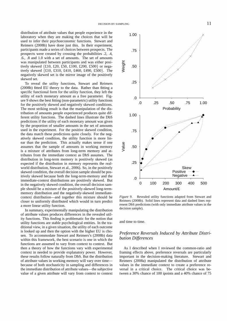
distribution of attribute values that people experience inthelaboratory when they are making the choices that will beused to infer their psychoeconomic functions. Stewart andReimers (2008b) have done just this. In their experiment,participants made a series of choices between prospects. Theprospects were created by crossing the probabilities .2, .4,.6., .8 and 1.0 with a set of amounts. The set of amountswas manipulated between participants and was either posi-tively skewed{£10, £20, £50, £100, £200, £500} or nega-tively skewed{£10, £310, £410, £460, £490, £500}. Thenegatively skewed set is the mirror image of the positivelyskewed set.

To reveal the utility functions, Stewart and Reimers(2008b) fitted EU theory to the data. Rather than fitting aspecific functional form for the utility function, they lefttheutility of each monetary amount as a free parameter. Fig-ure 9 shows the best fitting (non-parametric) utility functionsfor the positively skewed and negatively skewed conditions.The most striking result is that the manipulation of the dis-tribution of amounts people experienced produces quite dif-ferent utility functions. The dashed lines illustrate the DbSpredictions if the utility of each monetary amount was givenby the proportion of smaller amounts in the set of amountsused in the experiment. For the positive skewed condition,the data match these predictions quite closely. For the neg-atively skewed condition, the utility function is more lin-ear than the prediction. This actually makes sense if oneassumes that the sample of amounts in working memoryis a mixture of attributes from long-term memory and at-tributes from the immediate context as DbS assumes. Thedistribution in long-term memory is positively skewed (asexpected if the distribution in memory represents the real-world distribution, Stewart et al., 2006). So, in the positivelyskewed condition, the overall decision sample should be pos-itively skewed because both the long-term-memory and theimmediate-context distributions are positively skewed. Butin the negatively skewed condition, the overall decision sam-ple should be a mixture of the positively-skewed long-term-memory distribution and the negatively-skewed immediate-context distribution—and together this mixture should becloser to uniformly distributed which would in turn predicta more linear utility function.

In summary, experimentally manipulating the distributionof attribute values produces differences in the revealed util-ity functions. This finding is problematic for the notion thatutility functions are stable psychological entities. In the tra-ditional view, in a given situation, the utility of each outcomeis looked up and then the option with the higher EU is cho-sen. To accommodate Stewart and Reimers’s (2008b) datawithin this framework, the best scenario is one in which thefunctions are assumed to vary from context to context. Butthen a theory of how the functions vary with experimentalcontext in needed to provide explanatory power. However,these results follow naturally from DbS. But the distributionof attribute values in working memory will vary over time—because of both stochasticity in sampling and differences inthe immediate distribution of attribute values—the subjectivevalue of a given attribute will vary from context to context

1.00

.75

.50

.25

.0 0 100 200 300 400 500

Val

ue

Amount/£

SkewPositiveNegative

1.00

.75

.50

.25

.01.00.75.50.25.0

Wei

ght

Probability

Figure 9. Revealed utility functions adapted from Stewart andReimers (2008b). Solid lines represent data and dashed lines rep-resent DbS predictions (with only immediate attribute values in thedecision sample).

and time to time.

Preference Reversals Induced by Attribute Distri-bution Differences

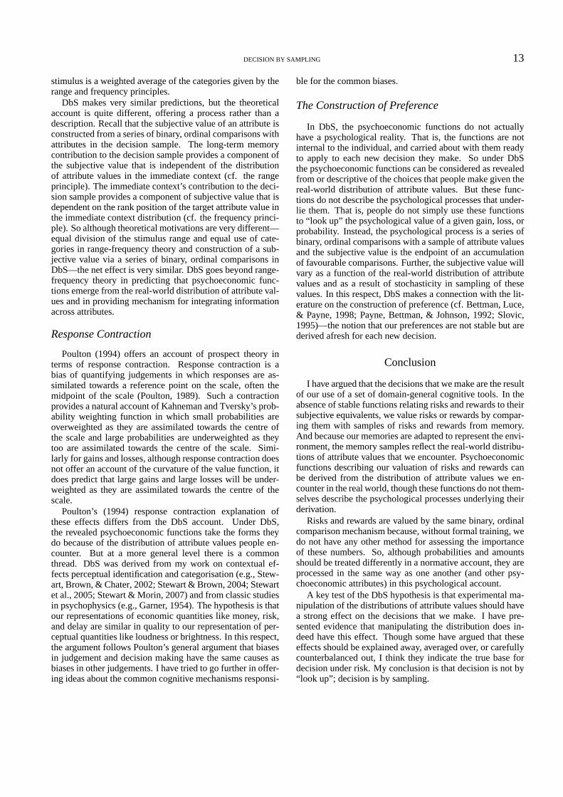
As I described when I reviewed the common-ratio andframing effects above, preference reversals are particularlyimportant in the decision-making literature. Stewart andReimers (2008a) manipulated the distribution of attributevalues in the immediate context to create a preference re-versal in a critical choice. The critical choice was be-tween a 30% chance of 100 ipoints and a 40% chance of 75

12 STEWART

ipoints.3 To set the context, this critical choice was precededby eight choices in which the distribution of attribute valueswas manipulated between participants. In the Probabilities-Together-Amounts-Apart Condition, the probabilities 10%,20%, 30%, 40%, 50%, and 60% were crossed with amounts75 ipoints, 80 ipoints, 85 ipoints, 90 ipoints, 95 ipoints,and 100 ipoints to create a set of prospects (100 ipointsare worth about £1). In the Probabilities-Apart-Amounts-Together Condition, the probabilities 30%, 32% , 34%, 36%,38%, and 40% were crossed with the amounts 25 ipoints, 50ipoints, 75 ipoints, 100 ipoints, 125 ipoints, and 150 ipoints.

The distribution of attributes in the Probabilities-Together-Amounts-Apart Condition was selected to makethe difference between the 30% and 40% in the criticalchoice appear small (with probabilities ranking 3rd and 4thin the distribution) while the difference between the 75ipoints and 100 ipoints was made to appear large (withamounts ranking 1st and 6th in the distribution). Thus, be-cause the difference in amounts is subjectively much largerthan the difference in probabilities, people should selectonthe basis of amount and choose the 30% chance of 100ipoints. The Probabilities-Apart-Amounts-Together Condi-tion reversed this manipulation, with probabilities ranking1st and 6th whilst amounts ranked 3rd and 4th. In this con-dition, people should select on the basis of probability andselect the 40% chance of 75 ipoints.

Figure 10 shows how the proportion of people select-ing each option in the critical choice varied by condition injust this way. The switch from a majority preference fora 30% chance of 100 ipoints in the Probabilities-Together-Amounts-Apart condition to a majority preference for a 40%chance of 75 ipoints in the Probabilities-Apart-Amounts-Together Condition represents an attribute-distributionin-duced preference reversal. Again, the conclusion is that wedo not have stable underlying psychoeconomic functions.The best case interpretation for the classical view is that thesefunctions are malleable and vary from context to context, butto go beyond the merely descriptive, one needs a theory toexplain why these functions vary from context to context.DbS provides an account of this sort - by abandoning stablepsychoeconomic functions and instead assuming that subjec-tive values are constructed afresh for each preference usingsimple cognitive tools.

Discussion

In the review, I have presented evidence that the subjectivevalue of a given risky option is not derived independently ofthe other options on offer. DbS offers one account of whythis might be the case. Because the decision sample con-tains attributes from the immediate context, the subjectivevalue of each attribute value will vary from context to con-text as the contents of the decision sample varies from con-text to context. In this way, DbS makes reference to threesignificant bodies of work: Parducci’s range-frequency the-ory, Poulton’s response-contraction explanation of prospecttheory, and Payne, Bettman, Johnson, Slovic and Luce’sconstruction-of-preference concept.

0

10

20

30

40

Probability-ApartAmount-Together

Probability-TogetherAmount-Apart

Fre

quen

cy o

f Sel

ectio

n

30% chance of 100 ipoints40% chance of 75 ipoints

Figure 10. A preference reversal for the choice 30% chance of 100or 40% chance of 75 ipoints Stewart and Reimers (2008b).

Range-Frequency Theory. Range-frequency theory (Par-ducci, 1965, 1995) is a theory of category judgement. Incategory judgement tasks, stimuli varying along a single di-mension are assigned one label from an ordered set of cate-gories (e.g., lines varying in their length might be assignedto categories “very short”, “short”, “medium”, “long”, “verylong”). Originally, the theory was used to account for theeffect of the distribution of perceptual stimuli on categoryjudgements. For example, a given target line length is ratedas larger in a positively skewed distribution of line lengths(i.e., many smaller lines) than in a negatively skewed dis-tribution of line lengths (i.e., many larger lines). Range-frequency theory has been applied very widely beyond thecategorisation of perceptual stimuli (see Parducci, 1995,fora review).4

Range-frequency theory has two components. The rangeprinciple states that the stimulus range is divided into equalsize categories (one for each category label) irrespectiveofthe distribution of stimuli. The frequency principle states thatthe stimulus range is divided into categories so that each cate-gory is used equally frequently and contains an equal numberof stimuli. Thus the division of the stimulus range under thefrequency principle is completely dependent on the distribu-tion of stimuli. For example, if line lengths are positivelyskewed, then the smaller lengths will be divided into manycategories and the larger lengths into fewer categories. Ef-fectively, under the frequency principle, the category labelassigned to a particular stimulus is determined by the stimu-lus’s rank position. The overall category assigned to a given

3 ipoints is an online reward scheme. ipoints can be redeemedfor a large range of goods.

4 Adaptation level theory (Helson, 1964) represents perhaps thefirst attempt to account for contextual effects. In adaptation leveltheory, stimuli are judged against the mean of the distribution inwhich they are encountered. Range-frequency theory goes furtherin accounting for the effects of higher moments, like the varianceand the skew.

DECISION BY SAMPLING 13

stimulus is a weighted average of the categories given by therange and frequency principles.

DbS makes very similar predictions, but the theoreticalaccount is quite different, offering a process rather than adescription. Recall that the subjective value of an attribute isconstructed from a series of binary, ordinal comparisons withattributes in the decision sample. The long-term memorycontribution to the decision sample provides a component ofthe subjective value that is independent of the distributionof attribute values in the immediate context (cf. the rangeprinciple). The immediate context’s contribution to the deci-sion sample provides a component of subjective value that isdependent on the rank position of the target attribute valueinthe immediate context distribution (cf. the frequency princi-ple). So although theoretical motivations are very different—equal division of the stimulus range and equal use of cate-gories in range-frequency theory and construction of a sub-jective value via a series of binary, ordinal comparisons inDbS—the net effect is very similar. DbS goes beyond range-frequency theory in predicting that psychoeconomic func-tions emerge from the real-world distribution of attributeval-ues and in providing mechanism for integrating informationacross attributes.

Response Contraction

Poulton (1994) offers an account of prospect theory interms of response contraction. Response contraction is abias of quantifying judgements in which responses are as-similated towards a reference point on the scale, often themidpoint of the scale (Poulton, 1989). Such a contractionprovides a natural account of Kahneman and Tversky’s prob-ability weighting function in which small probabilities areoverweighted as they are assimilated towards the centre ofthe scale and large probabilities are underweighted as theytoo are assimilated towards the centre of the scale. Simi-larly for gains and losses, although response contraction doesnot offer an account of the curvature of the value function, itdoes predict that large gains and large losses will be under-weighted as they are assimilated towards the centre of thescale.

Poulton’s (1994) response contraction explanation ofthese effects differs from the DbS account. Under DbS,the revealed psychoeconomic functions take the forms theydo because of the distribution of attribute values people en-counter. But at a more general level there is a commonthread. DbS was derived from my work on contextual ef-fects perceptual identification and categorisation (e.g.,Stew-art, Brown, & Chater, 2002; Stewart & Brown, 2004; Stewartet al., 2005; Stewart & Morin, 2007) and from classic studiesin psychophysics (e.g., Garner, 1954). The hypothesis is thatour representations of economic quantities like money, risk,and delay are similar in quality to our representation of per-ceptual quantities like loudness or brightness. In this respect,the argument follows Poulton’s general argument that biasesin judgement and decision making have the same causes asbiases in other judgements. I have tried to go further in offer-ing ideas about the common cognitive mechanisms responsi-

ble for the common biases.

The Construction of Preference

In DbS, the psychoeconomic functions do not actuallyhave a psychological reality. That is, the functions are notinternal to the individual, and carried about with them readyto apply to each new decision they make. So under DbSthe psychoeconomic functions can be considered as revealedfrom or descriptive of the choices that people make given thereal-world distribution of attribute values. But these func-tions do not describe the psychological processes that under-lie them. That is, people do not simply use these functionsto “look up” the psychological value of a given gain, loss, orprobability. Instead, the psychological process is a series ofbinary, ordinal comparisons with a sample of attribute valuesand the subjective value is the endpoint of an accumulationof favourable comparisons. Further, the subjective value willvary as a function of the real-world distribution of attributevalues and as a result of stochasticity in sampling of thesevalues. In this respect, DbS makes a connection with the lit-erature on the construction of preference (cf. Bettman, Luce,& Payne, 1998; Payne, Bettman, & Johnson, 1992; Slovic,1995)—the notion that our preferences are not stable but arederived afresh for each new decision.

Conclusion

I have argued that the decisions that we make are the resultof our use of a set of domain-general cognitive tools. In theabsence of stable functions relating risks and rewards to theirsubjective equivalents, we value risks or rewards by compar-ing them with samples of risks and rewards from memory.And because our memories are adapted to represent the envi-ronment, the memory samples reflect the real-world distribu-tions of attribute values that we encounter. Psychoeconomicfunctions describing our valuation of risks and rewards canbe derived from the distribution of attribute values we en-counter in the real world, though these functions do not them-selves describe the psychological processes underlying theirderivation.

Risks and rewards are valued by the same binary, ordinalcomparison mechanism because, without formal training, wedo not have any other method for assessing the importanceof these numbers. So, although probabilities and amountsshould be treated differently in a normative account, they areprocessed in the same way as one another (and other psy-choeconomic attributes) in this psychological account.

A key test of the DbS hypothesis is that experimental ma-nipulation of the distributions of attribute values shouldhavea strong effect on the decisions that we make. I have pre-sented evidence that manipulating the distribution does in-deed have this effect. Though some have argued that theseeffects should be explained away, averaged over, or carefullycounterbalanced out, I think they indicate the true base fordecision under risk. My conclusion is that decision is not by“look up”; decision is by sampling.

14 STEWART

References

Allais, M. (1953). Le comportement de l’homme rationel devantle risque: Critique des postulats et axioms de l’ecole americaine[Rational man’s behavior in face of risk: Critique of the Amer-ican School’s postulates and axioms].Econometrica, 21, 503–546.

Anderson, J. R., & Schooler, L. J. (1991). Reflections of the envi-ronment in memory.Psychological Science, 2, 396–408.

Anderson, N. H. (1981).Foundations of information integrationtheory. New York: Academic Press.

Ariely, D., Koszegi, B., Mazar, N., & Shampan’er, K. (n.d.).Price-sensitive preferences.Unpublished manuscript.

Bak, P. (1997).How nature works: The science of self-organizedcriticality. Oxford, UK: Oxford University Press.

Bell, D. E., & Fishburn, P. C. (1999). Utility functions for wealth.Journal of Risk and Uncertainty, 20, 5–44.

Benartzi, S., & Thaler, R. H.(2001). Naive diversification strategiesin defined contribution saving plans.The American EconomicReview, 91, 79–98.

Bernoulli, D. (1954). Expositions of a new theory of the measure-ment of risk. Econometrica, 22, 23–36. (Original work pub-lished 1738)

Bettman, J. R., Luce, M. F., & Payne, J. W. (1998). Constructiveconsumer choice processes.Journal of Consumer Research, 25,187–217.

Birnbaum, M. H.(1992). Violations of the monotonicity and contex-tual effects in choice-based certainty equivalents.PsychologicalScience, 3, 310–314.

Birnbaum, M. H. (2008). New paradoxes of risky decision making.Psychological Review, 115, 453–501.

Birnbaum, M. H., & Chavez, A. (1997). Tests of theories of de-cision making: Violations of branch independence and distribu-tion independence.Organizational Behavior and Human Deci-sion Processes, 71, 161–194.

Brown, G. D. A., Gardner, J., Oswald, A. J., & Qian, J.(2008). Doeswage rank affect employees’ well-being?Industrial Relations,47, 355–389.

Budescu, D. V., & Wallsten, T. S. (1995). Processing linguisticprobabilities: General principles and empirical evidence. InJ. Busemeyer, D. L. Medin, & R. Hastie (Eds.),The psychologyof learning and motivation: Vol. 32. Decision making from acognitive perspective(pp. 275–318). San Diego, CA: AcademicPress.

Busemeyer, J. R., & Townsend, J. T. (1993). Decision field theory:A dynamic-cognitive approach to decision making in an uncer-tain environment.Psychological Review, 100, 432–459.

Camerer, C. F. (1995). Individual decision making. In J. Kagel& A. E. Roth (Eds.),Handbook of experimental economics(pp.587–703). Princeton, NJ: Princeton University Press.

Carlin, P. S. (1992). Violations of the reduction and indepen-dence axioms in Allais-type and common-ratio effect experi-ments.Journal of Economic Behavior & Organization, 19, 213–235.

Chater, N., & Brown, G. D. A. (2008). From universal laws ofcognition to specific cognitive models.Cognitive Science, 32,36–47.

Daniels, R. L., & Keller, L. R. (1992). Choice-based assessment ofutility functions.Organizational Behavior and Human DecisionProcesses, 52, 524–543.

Davies, G. B., & Satchell, S. E. (2007). The behavioural compo-nents of risk aversion.Journal of Mathematical Psychology, 51,1–13.

Dawes, R. M.(1979). The robust beauty of linear models of decisionmaking.American Psychologist, 34, 571–582.

Dhar, R., & Glazer, R. (1996). Similarity in context: Cognitiverepresentation and violation of preference and perceptual invari-ance in consumer choice.Organizational Behavior and HumanDecision Processes, 67, 280–293.

Dougherty, M. P. R., & Hunter, J. (2003a). Hypothesis genera-tion, probability judgment, and individual differences in work-ing memory capacity.Acta Psychologica, 113, 263–282.

Dougherty, M. P. R., & Hunter, J. (2003b). Probability judgmentand subadditivity: The role of working memory capacity andconstraining retrieval.Memory & Cognition, 31, 968–982.

Edwards, W. (1962). Subjective probabilities inferred from deci-sions.Psychological Review, 69, 109–135.

Engle, R. W., Tuholski, S. W., Laughlin, J. E., & Conway, A. R. A.(1999). Working memory, short term memory, and general fluidintelligence: A latent variable approach.Journal of Experimen-tal Psychology: General, 128, 309–331.

Ert, E., & Erev, I. (2007). Loss aversion in decisions under riskand the value of a symmetric simplification of prospect theory.Unpublished manuscript.

Feller, W. (1968). An introduction to probability theory and itsapplications(Vol. 1). New York: Wiley.

Fishburn, P. C., & Kochenberger, G. A. (1979). Two-piece vonNeumann-Morgenstern utility functions.Decision Sciences, 10,503–518.

Galanter, E. (1962). The direct measurement of utility and subjec-tive probability.American Journal of Psychology, 75, 208–220.

Galanter, E. (1990). Utility functions for nonmonetary events.American Journal of Psychology, 103, 449–470.

Garner, W. R. (1954). Context effects and the validity of loudnessscales.Journal of Experimental Psychology, 48, 218–224.

Gigerenzer, G., & Hoffrage, U. (1995). How to improve Bayesianreasoning without instruction: Frequency formats.Psychologi-cal Review, 102, 684–704.

Gonzalez, R., & Wu, G. (1999). On the shape of the probabilityweighting function.Cognitive Psychology, 38, 129–166.

Helson, H. (1964).Adaptation-level theory. New York: Harper &Row.

Huber, J., Payne, J. W., & Puto, C. (1982). Adding asymmetricallydominated alternatives: Violations of regularity and the similar-ity hypothesis.Journal of Consumer Research, 9, 90–98.

Kahneman, D., & Miller, D. T. (1986). Norm theory: Comparingreality to its alternatives.Psychological Review, 93, 136–153.

Kahneman, D., & Tversky, A.(1979). Prospect theory: An analysisof decision under risk.Econometrica, 47, 263–291.

Kahneman, D., & Tversky, A. (Eds.). (2000).Choices, values andframes. New York: Cambridge University Press & the RussellSage Foundation.

Kornbrot, D. E., Donnelly, M., & Galanter, E. (1981). Estimates ofutility function parameters from signal-detection experiments.Journal of Experimental Psychology: Human Perception andPerformance, 7, 441–458.

Laming, D. R. J. (1997).The measurement of sensation. London:Oxford University Press.

DECISION BY SAMPLING 15

Levin, I. R., Johnson, R. D., Russo, C. P., & Delden, P. J. (1985).Framing effects in judgment tasks with varying amounts of in-formation. Organizational Behavior and Human Decision Pro-cesses, 36, 362–377.

Loomes, G., & Sugden, R. (1982). Regret theory: An alternativetheory of rational choice under uncertainty.Economic Journal,92, 805–824.

Lopes, L. L., & Oden, G. C. (1983). Some thoughts on the psycho-logical concept of risk. Journal of Experimental Psychology:Human Perception and Performance, 9, 137–144.

Luce, R. D. (2000). Utility of gains and losses: Measurement-theoretical and experimental approaches. Mahwah, NJ: Erl-baum.

Mellers, B. A., & Chang, S. (1994). Representations of risk judg-ments. Organizational Behavior and Human Decision Pro-cesses, 57, 167–184.

Mellers, B. A., Chang, S. J., Birnbaum, M. H., & Ordonez, L. D.(1992). Preferences, prices, and ratings in risky decision-making. Journal of Experimental Psychology: Human Percep-tion and Performance, 18, 347–361.

Mellers, B. A., Ordonez, L. D., & Birnbaum, M. H. (1992). Achange-of-process theory for contextual effects and preferencereversals in risky decision making.Organizational Behavior andHuman Decision Processes, 52, 331–369.

Parducci, A.(1965). Category judgment: A range-frequency model.Psychological Review, 72, 407–418.

Parducci, A. (1995).Happiness, pleasure and judgment: The con-textual theory and its applications. Mahwah, NJ: Erlbaum.

Payne, J. W., Bettman, J. R., & Johnson, E. J.(1992). Behavioralde-cision research: A constructive processing perspective.AnnualReview of Psychology, 43, 87–131.

Poulton, E. C.(1989).Bias in quantifying judgments. Hillsdale, NJ:Erlbaum.

Poulton, E. C. (1994).Behavioural decision theory: A new ap-proach. Cambridge, England: Cambridge University Press.

Quiggin, J. (1993).Generalized expected utility theory: The rank-dependent model. Norwell, MA: Kluwer Academic Publishers.

Savage, L. J. (1954).The foundations of statistics. New York:Wiley.

Schoemaker, P. J. H. (1982). The expected utility model: Its vari-ants, purposes, evidence, and limitations.Journal of EconomicLiterature, 20, 529–563.

Sedlmeier, P., & Betsch, T. (Eds.). (2002).Etc. Frequency process-ing and cognition. Oxford, England: Oxford University Press.

Shanteau, J. (1975). Averaging versus multiplying combinationrules of inference judgment.Acta Psychologica, 39, 83–89.

Simonson, I. (1989). Choice based on reasons: The case of attrac-tion and compromise effects.Journal of Consumer Research,16, 158–174.

Slovic, P. (1995). The construction of preference.American Psy-chologist, 50, 364–371.

Sprenger, A., & Dougherty, M. R. (2006). Differences betweenprobability and frequency judgments: The role of individual dif-ferences in working memory capacity.Organizational Behaviorand Human Decision Processes, 99, 202–211.

Starmer, C. (2000). Developments in non-expected utility theory:The hunt for a descriptive theory of choice under risk.Journalof Economic Literature, 38, 332–382.

Stewart, N., & Brown, G. D. A. (2004). Sequence effects in cat-egorizing tones varying in frequency.Journal of ExperimentalPsychology: Learning, Memory, and Cognition, 30, 416–430.

Stewart, N., Brown, G. D. A., & Chater, N. (2002). Sequence ef-fects in categorization of simple perceptual stimuli.Journal ofExperimental Psychology: Learning, Memory, and Cognition,28, 3–11.

Stewart, N., Brown, G. D. A., & Chater, N.(2005). Absolute identi-fication by relative judgment.Psychological Review, 112, 881–911.

Stewart, N., Chater, N., & Brown, G. D. A. (2006). Decision bysampling.Cognitive Psychology, 53, 1–26.

Stewart, N., Chater, N., Stott, H. P., & Reimers, S.(2003). Prospectrelativity: How choice options influence decision under risk.Journal of Experimental Psychology: General, 132, 23–46.

Stewart, N., & Morin, C. (2007). Dissimilarity is used as evi-dence of category membership in multidimensional perceptualcategorisation: A test of the similarity-dissimilarity generalisedcontext model.Quarterly Journal of Experimental Psychology,60, 1337–1346.

Stewart, N., & Reimers, S.(2008a).How the distribution of attributevalues influences decision under risk.Unpublished manuscript.

Stewart, N., & Reimers, S.(2008b).Revealed psychoeconomic func-tions are not stable.Unpublished manuscript.

Stewart, N., & Simpson, K. (2008). A decision-by-sampling ac-count of decision under risk. In N. Chater & M. Oaksford (Eds.),The probabilistic mind: Prospects for Bayesian cognitive sci-ence(pp. 261–276). Oxford, England: Oxford University Press.

Stott, H. P. (2006). Cumulative prospect theory’s functionalmenagerie.Journal of Risk and Uncertainty, 32, 101–130.

Thomas, R. P., Dougherty, M. R. P., Sprenger, A. M., & Harbison,J. I. (2008). Diagnostic hypothesis generation and human judg-ment.Psychological Review, 115, 155–185.

Tversky, A. (1969). Intransitivity of preferences.PsychologicalReview, 76, 31–48.

Tversky, A., & Kahneman, D.(1992). Advances in prospect theory:Cumulative representation of uncertainty.Journal of Risk andUncertainty, 5, 297–323.

Tversky, A., & Koehler, D. J. (1994). Support theory: A nonex-tensional representation of subjective probability.PsychologicalReview, 101, 547–567.

Vlaev, I., Chater, N., & Stewart, N. (2007a). Financial prospect rel-ativity: Context effects in financial decision-making under risk.Journal of Behavioral Decision Making, 20, 273–304.

Vlaev, I., Chater, N., & Stewart, N. (2007b). Relativistic financialdecisions: Context effects on retirement saving and investmentrisk preferences.Judgment and Decision Making, 2, 292–311.

von Neumann, M., & Morgenstern, O.(1947).Theory of games andeconomic behavior(2nd ed.). Princeton, NJ: Princeton Univer-sity Press.

Wedell, D. H.(1991). Distinguishing among models of contextuallyinduced preference reversals.Journal of Experimental Psychol-ogy: Learning, Memory, and Cognition, 17, 767–778.

Windschitl, P. D., & Chambers, J. R. (2004). The dud-alternativeeffect in likelihood judgment.Journal of Experimental Psychol-ogy: Learning, Memory, and Cognition, 30, 198–215.

Windschitl, P. D., & Wells, G. L. (1998). The alternative-outcomeseffect. Journal of Personality and Social Psychology, 75, 1441–1423.