Financial Prospect Relativity: Context Effects in Financial Decision-Making Under Risk y IVO VLAEV 1 * , NICK CHATER 1 and NEIL STEWART 2 1 Department of Psychology, University College London, London, UK 2 Department of Psychology, University of Warwick, Coventry, UK ABSTRACT We report three studies in which methodologies from psychophysics are adapted to investigate context effects on individual financial decision-making under risk. The aim was to determine how the range and the rank of the options offered as saving amounts and levels of investment risk influence people’s decisions about these variables. In the range manipulation, participants were presented with either a full range of choice options or a limited subset, while in the rank manipulation they were presented with a skewed set of feasible options. The results showed that choices are affected by the position of each option in the range and the rank of presented options, which suggests that judgments and choices are relative. Copyright # 2006 John Wiley & Sons, Ltd. key words prospect relativity; decision-making; judgment; investment risk; saving decisions; context effects; perception INTRODUCTION Two goals of the research are presented here: the first is theoretical, while the second is applied. The theoretical goal is to test the robustness of empirical phenomena in judgment and decision-making research, which concern the context malleability of human decision-making under risk. The applied objective of the three experiments outlined below is to develop ways of stimulating financial consumers to save more for retirement and be less risk averse in relation to their retirement savings investments. This objective is in consumers’ interest and relates to government concerns that people in the UK and other industrialized countries save too little and do not take enough financial risk (e.g., Oliver, Wyman & Company, 2001). Our article presents laboratory experiments in which investment decisions were manipulated by the context in which they were presented. In particular, our research focused on studying the effects of the choice option set when asking people to express their preferences in relation to different retirement savings and investment scenarios. The crucial Journal of Behavioral Decision Making J. Behav. Dec. Making, 20: 273–304 (2007) Published online 30 November 2006 in Wiley InterScience (www.interscience.wiley.com) DOI: 10.1002/bdm.555 *Correspondence to: Ivo Vlaev, Department of Psychology, University College London, London, WC1H 0AP, UK. E-mail: [email protected] y The data in this paper were collected while Ivo Vlaev was a doctoral student at the Department of Experimental Psychology, University of Oxford. Copyright # 2006 John Wiley & Sons, Ltd.

Welcome message from author
This document is posted to help you gain knowledge. Please leave a comment to let me know what you think about it! Share it to your friends and learn new things together.
Transcript
Financial Prospect Relativity: Context Effectsin Financial Decision-Making Under Risky
IVO VLAEV1*, NICK CHATER1 and NEIL STEWART2
1Department of Psychology, University College London, London, UK2Department of Psychology, University of Warwick, Coventry, UK
ABSTRACT
We report three studies in which methodologies from psychophysics are adapted toinvestigate context effects on individual financial decision-making under risk. The aimwas to determine how the range and the rank of the options offered as saving amountsand levels of investment risk influence people’s decisions about these variables. In therange manipulation, participants were presented with either a full range of choiceoptions or a limited subset, while in the rank manipulation they were presented with askewed set of feasible options. The results showed that choices are affected by theposition of each option in the range and the rank of presented options, which suggeststhat judgments and choices are relative. Copyright # 2006 John Wiley & Sons, Ltd.
key words prospect relativity; decision-making; judgment; investment risk; saving
decisions; context effects; perception
INTRODUCTION
Two goals of the research are presented here: the first is theoretical, while the second is applied. The
theoretical goal is to test the robustness of empirical phenomena in judgment and decision-making research,
which concern the context malleability of human decision-making under risk. The applied objective of the
three experiments outlined below is to develop ways of stimulating financial consumers to save more for
retirement and be less risk averse in relation to their retirement savings investments. This objective is in
consumers’ interest and relates to government concerns that people in the UK and other industrialized
countries save too little and do not take enough financial risk (e.g., Oliver, Wyman & Company, 2001). Our
article presents laboratory experiments in which investment decisions were manipulated by the context in
which they were presented.
In particular, our research focused on studying the effects of the choice option set when asking people to
express their preferences in relation to different retirement savings and investment scenarios. The crucial
Journal of Behavioral Decision Making
J. Behav. Dec. Making, 20: 273–304 (2007)
Published online 30 November 2006 in Wiley InterScience
(www.interscience.wiley.com) DOI: 10.1002/bdm.555
*Correspondence to: Ivo Vlaev, Department of Psychology, University College London, London, WC1H 0AP, UK.E-mail: [email protected] data in this paper were collected while Ivo Vlaev was a doctoral student at the Department of Experimental Psychology, Universityof Oxford.
Copyright # 2006 John Wiley & Sons, Ltd.
practical question here is how to enable people to make better investment decisions, by presenting the
financial information in such a way that they are motivated to save more and encouraged to increase the
proportion of investments in risky products. The experimental design and method are based on the prospect
relativity phenomenon (Stewart, Chater, Stott, & Reimers, 2003) and the rank dependence effect (Birnbaum,
1992), both of which demonstrate the dependence of human preferences and decisions on the set of choice
options they are presented with, and the lack of stable underlying preference function. The robustness and
practical relevance of these two phenomena can, therefore, be better assessed in the light of the results
obtained with realistic decision situations used here, as opposed to the abstract choice scenarios with which
both effects were initially tested.
PREVIOUS EXPERIMENTAL RESEARCH
Much of human behavior is a consequence of decision-making which involves some judgment of the
potential rewards and risk associated with each action. Deciding how to invest one’s savings, for example,
involves balancing the risks and likely returns of the prospects available. Understanding how people trade-off
financial risk and return and make choices on the basis of these trade-offs is a central question for both
psychology and economics, because the foundations of economic theory are rooted in models of individual
decision-making. So in order to explain the behavior of investors, we need a model of the decision-making
behavior under risk and uncertainty.
Most of economic theory has been based on a normative theory of decision-making under risk and
uncertainty, expected utility theory, first axiomatized by von Neumann and Morgenstern (1947). Expected
utility theory specifies certain axioms of rational choice, and then shows that if people obey these axioms,
they can be characterized as having a cardinal utility function. In essence, people are assumed to make
choices that maximize their utility, and they value a risky option or a strategy by the expected utility this
option will provide (the expected utility is modeled as the expected payoffs weighted by their respective
probabilities). Deviations of real behaviors from this theory have been seen as primarily due to lack of
experience and opportunity for learning, confusion, and lack of enough information (see Shafir & LeBoeuf,
2002, for discussion). Psychologists and economists have been trying to empirically verify the assumptions of
rational choice theory, revealing ever increasing evidence that human behavior diverges from the predictions
of the theory (e.g., Kagel & Roth, 1995; Kahneman & Tversky, 2000; and also Camerer, 1995, for a review).
Loomes (1999) suggests that the evidence accumulated so far in the literature is much more easily
reconciled with a world where most individuals have only rather basic and fuzzy preferences (even for quite
familiar sums of money). This evidence is contrary to the fundamental rational choice assumption that
individuals have reasonably well-articulated values that are successfully applied to all types of decision tasks.
The view that each version of the decision problem triggers its own preference elicitation is similar to the
claim that preferences are constructed, (i.e., not elicited or revealed), in the generation of a response to a
judgment or choice task (Bettman, Luce, & Payne, 1998; Fischhoff, 1991; Slovic, 1995; Tversky, Sattath, &
Slovic, 1988).
Effects of the choice set have been demonstrated in consumer choice (i.e., trade-offs without risk) and the
basic finding is that the choice set can influence how much variety consumers select (Simonson, 1990).
Simonson suggests that this behavior might be explained by variety seeking serving as a choice heuristic.
That is, when asked to make several choices at once, people tend to diversify. This result has been called the
diversification bias by Read and Loewenstein (1995). Benartzi and Thaler (1998, 2001) have found evidence
of the same phenomenon by studying how people allocate their retirement funds across various investment
vehicles. In particular, they find some evidence for an extreme version of this bias that they call the 1/n
heuristic. The idea is that when an employee is offered n funds to choose from in her retirement plan, she
divides the money evenly among the funds offered. Use of this heuristic, or others even more sophisticated,
Copyright # 2006 John Wiley & Sons, Ltd. Journal of Behavioral Decision Making, 20, 273–304 (2007)
DOI: 10.1002/bdm
274 Journal of Behavioral Decision Making
implies that the asset allocation an investor chooses will depend strongly on the array of funds offered in the
retirement plan. Thus, in a plan that offered one stock fund and one bond fund, the average allocation would
be 50% stocks, but if another stock fund were added, the allocation to stocks would jump to two-thirds.
Benartzi and Thaler found evidence supporting just this behavior in real-world pension choices. In a sample
of US 401 k pension plans, they regressed the percentage of the plan assets invested in stocks on the
percentage of the funds that were stock funds and found a very strong relationship. Note that these are
real-world data on the distribution of assets across pension funds with different levels of risk (i.e., different
numbers of stocks and bonds offered by each particular employer) and thus, this study creates a natural
experiment that allows us to compare the effects of offering more stocks and fewer bonds versus fewer stocks
and more bonds. The results showing the strong effect of the choice set on actual behavior highlight difficult
issues regarding the design of retirement saving plans, both public and private,1 as it is not clear that people
can consistently select a ‘‘preferred’’ mix of fixed income and equity funds. For example, Benartzi and Thaler
point out that if the plan offers many fixed-income funds, the participants might invest too conservatively,
while if the plan offers many equity funds, the employees might invest too aggressively.
The findings by Benartzi and Thaler (1998, 2001) illustrate that investors have ill-formed preferences
about their investments, which again is consistent with the idea that preferences are constructed (Slovic,
1995). In another study, Benartzi and Thaler (2002) asked individuals to choose among investment programs
that offer different ranges of retirement income (for instance, a certain amount of $900 per month vs. a 50–50
chance to earn either $1100 per month or $800 per month). When they presented individuals with three
choices ranging from low risk to high risk, they found a significant tendency to pick the middle choice. For
instance, people viewing choices A, B, and C, will often find B more attractive than C. However, those
viewing choices B, C, and D, will often argue that C is more attractive than B. Simonson and Tversky (1992)
illustrated similar behavior in the context of consumer choice, which they dubbed extremeness aversion and
also the compromise effect. These results confirm that choices between alternatives depend on other
irrelevant options available. This again illustrates that choices are not rational according to standard
economic criteria and when choice problems are difficult, people may resort to simple ‘‘rules of thumb’’ to
help them cope, such as the rule that it is best to avoid extremes.
Several other studies have also shown similar types of effects. For example, the range of frequencies in
response options (measures of frequency of behavior or other events) can have an effect on the response
process, and on answers to questions that follow (e.g., Menon, Raghubir, & Schwarz, 1995; Schwarz &
Bienias, 1990; Schwarz, Hippler, Deutsch, & Strack, 1985). For example, in an experimental investigation of
response option ranges in a ‘‘somatic complaints’’ scale, respondents who were presented with a high
frequency range of responses (from ‘‘4 or less’’ to ‘‘9 or more’’) were much more likely to report feeling ‘‘low
or emotionally depressed’’ on five or more occasions during the past month than respondents presented with
the low range of response options (from ‘‘0’’ to ‘‘5 or more’’; Harrison & McLaughlin, 1996). Apparently,
the response ranges in this example must have influenced respondents’ interpretation of the intensity of
emotional experience. Similar effects were observed in responses to the nine other items of the scale. In
general, such bias effects appear in a wide range of experimental contexts. For example, even such a basic
quality like the perceived size of a physical object systematically varies with the method of measurement
(Poulton, 1989), which can be numerical estimates, drawings, or matching something to a variable target.
Our research presented here is based on a particular study of constructed risk preferences conducted by
Stewart et al. (2003) who tested whether the attributes of risky prospects behave like those of perceptual
1Diversification bias can be costly because investors might pick thewrong point along the frontier. Brennan and Torous (1999) consideredan individual with a coefficient of relative risk aversion of 2, which is consistent with the empirical findings of Friend and Blume (1975),and then calculated that the loss of welfare from picking portfolios that do not match the assumed risk preferences is 25% in a 20-yearinvestment horizon and 35–40% for 30 years horizon. For an individual who is less risk averse and has a coefficient of 1.0, the welfarecosts of investing too little in equities can be even larger.
Copyright # 2006 John Wiley & Sons, Ltd. Journal of Behavioral Decision Making, 20, 273–304 (2007)
DOI: 10.1002/bdm
I. Vlaev et al. Financial Prospect Relativity 275
stimuli and found similar context effects between decision-making under risk and perceptual identification.
Their experiments demonstrated the notable effect of the available options set, suggesting that prospects of
the form ‘‘p chance of x’’ are valued relative to one another. The idea behind this experiment was that some of
the factors that determine how people assess magnitudes like payoff and probability might be analogous to
factors underlying an assessment of psychophysical magnitudes, such as loudness or weight. Specifically,
psychophysical experiments have shown that people cannot provide stable absolute judgments of such
magnitudes, and are heavily influenced by the options available to them (Garner, 1954; Laming, 1997). In
particular, Stewart et al. found that the set of options from which an option was selected almost completely
determined the choice. They demonstrated this effect in a certainty equivalent estimation task (the amount of
money for certain that is worth the same to the person as a single chance to play the prospect) and in the
selection of a risky prospect.
There have been other experiments that have also investigated the effect of the set of available options in
decision under risk. Birnbaum (1992) demonstrated that the skew of the distribution of options offered as
certainty equivalents for simple prospects (while the maximum and minimum are held constant) influences
the selection of a certainty equivalent. In particular, prospects were less valued in the positively skewed
option set where most values were small, compared to when the options were negatively skewed and hence
most values were large. Similar results were obtained by Mellers, Ordonez, and Birnbaum (1992) who
measured participants’ attractiveness ratings and buying prices (to obtain the opportunity to play the prospect
for real and have a chance to receive the outcome) for a set of simple binary prospects of the form ‘‘p chance
of x.’’
The experiments by Birnbaum (1992) and Stewart et al. (2003) still lack, however, the link with the
real-world context in which people make the actual risky choices that are relevant to their financial futures.
This gap motivated us to investigate whether using decision situations that people encounter in their real lives
would produce effects similar to Birnbaum’s and Stewart et al.’s findings. In the three experiments reported
below, we found large and systematic effects of choice set (consisting of alternative saving and investment
prospects) on the choice of saving and investment plans. These effects are compatible with the prospect
relativity hypothesis proposed by Stewart et al. and also those models that discard the assumption that the
value of a choice option is independent of other available options (contrary to standard models of rational
choice).
In summary, the findings presented above show the importance of the effects of the choice set on people’s
preferences in various decision domains. One natural way to attempt to explain these effects is by assuming
that people’s representations of the relevant dimensions (e.g., level of risk) are not stable, but are influenced
by context. Two classic theories, originating from the psychophysical literature, have been proposed to
explain this type of effect—adaptation level theory (Helson, 1964) and range–frequency theory (Parducci,
1965, 1974). As we shall see below, both of these accounts of the contextual dependency of judgment can be
used as the foundation for explaining context effects in choice; and we shall model the data gathered in this
paper using implementations of both types of model.
Adaptation level theory is based on the assumption that judgments, for example, of loudness, brightness,
or, here, say, riskiness, are not absolute but relative to an ‘‘adaptation level,’’ which is a weighted sum of
recent stimuli. Thus, an option is viewed as risky not by comparison with any absolute standard, but in
relation to other recently encountered stimuli. Intuitively, the idea is that the perceptual or cognitive system
‘‘adapts’’ to the values of recent stimuli, and the subjective judgment of the magnitude of a new stimulus is
made in comparison with this adaptation level. Note, in particular, that by focusing on the adaptation level
(which will be related to an average of the distribution of recent items), the account assumes that there is no
direct impact of other aspects of the distribution of past items, such as variance, skew, and range.
Range–frequency theory, by contrast, predicts that the subjective value given to a magnitude is a function
of its position within the overall range and rank of distribution of magnitudes that have been observed.
Specifically, the impact of range is captured by expressing the current magnitude as a fraction of the interval
Copyright # 2006 John Wiley & Sons, Ltd. Journal of Behavioral Decision Making, 20, 273–304 (2007)
DOI: 10.1002/bdm
276 Journal of Behavioral Decision Making
from the lowest to the highest magnitude that has been encountered. This fraction will be a number between
0 and 1. The impact of rank is captured by the rank position of the item, in relation to the distribution of all
contextually relevant items and this rank position is also normalized to be between 0 and 1. The predictions of
range–frequency theory are then obtained by a weighted average of these quantities, where the relative
contribution of the two is a free parameter.
Parducci (1965, 1974) developed range–frequency theory as an alternative to adaptation level theory, to
account for his observation that the neutral point of the scale does not correspond to the mean of the
contextual events, as adaptation level theory predicts (Helson, 1964), but rather to a compromise between the
midpoint and median of the distribution of contextual events. The contribution of the midpoint, for Parducci,
is captured by measuring the range of the distribution; the contribution of the median is measured by
capturing rank.
Both adaptation level and range–frequency theory assume that people judge magnitudes not according to
any absolute scale, but in relation to other contextually relevant magnitudes. Both theories imply that
judgments will be invariant to certain transformations of the stimuli. In particular, if all stimuli in an auditory
experiment are increased or decreased in intensity by, say, ten decibels, the relative positions of the stimuli
will be unchanged, and according to both theories judgments concerning those stimuli should be identical.
(Of course, influences of absolute stimulus intensity can still be accounted for, either by noting that there is
implicit comparison with extrinsic stimuli, such as ambient noise, or internal noises, e.g., from within the
listener’s body; and that invariance to such transformations breaks down at extremes, where the perceptual
apparatus does not function effectively e.g., where the stimulus is inaudible).
Range–frequency theory also predicts that there should be no effect of the variance of the stimuli—that is,
it assumes that if the spacing between stimuli were increased by, for example, a factor of two, people’s
judgments of the relevant magnitudes would be unchanged. This is because each stimulus is evaluated by the
range of items and the rank position of each item, and these quantities are not modified by linearly stretching
out, or compressing, the items. Range–frequency theory, unlike adaptation level theory, does predict that
changing the skew of a distribution, while leaving its mean invariant, will affect judgments. For example, the
midpoint of the rangewill be perceived as ‘‘greater’’ for a negatively skewed distribution (because most items
will be below it in rank position), whereas it will be perceived as ‘‘lower’’ for a positively skewed distribution
(because most items will be above it in rank position).
How can these theories of the impact of context on judgment be employed to explain how context can
affect the choices people make between options. We follow previous work (e.g., Wedell & Pettibone, 1999) in
proposing that judgment affects attractiveness—and that attractiveness in trade-offs (such as the trade-off
between risk and return) can be viewed as depending on the nearness to a single ‘‘ideal’’ standard. The
probability of choosing an option is then assumed to be proportional to the attractiveness of that option. (This
is Luce’s (1959) choice rule, in its simplest form. See below.)
The classical ideal point approach proposed by Coombs (1964) falls into this category of models of
attractiveness (see also Riskey, Parducci, & Beauchamp, 1979; Wedell & Pettibone, 1999). According to this
model, people represent ‘‘ideal points’’ and judge the attractiveness of a stimulus by its distance from the
ideal point. Norm theory (Kahneman &Miller, 1986) follows a similar approach. However, the standard here
is called the ‘‘norm’’ and is constructed on the spot rather than retrieved from long-term memory. (A
comparison set is constructed in working memory, consisting of known exemplars, and its norm is computed,
usually by deriving the mean of the presented values and the context is usually assumed to shift the ideal
towards this mean.) In norm theory, as indeed in adaptation level theory, there is no assumption that the
‘‘standard’’ is preferred—that is, viewed as the most attractive option.
Ideal point models appear promising in the present context, because attractiveness in the context of
trade-offs may naturally be viewed as involving something akin to a bell-shaped relationship between
attractiveness and the trade-off between trade-off stimulus dimensions (here, saving and risk). In other words,
more saving and risk is not always better and the relationship between preference and value in these two
Copyright # 2006 John Wiley & Sons, Ltd. Journal of Behavioral Decision Making, 20, 273–304 (2007)
DOI: 10.1002/bdm
I. Vlaev et al. Financial Prospect Relativity 277
domains is characterized by a single-peaked preference curve in which the ideal lies at an intermediate value
between the extremes. Too much risk is not attractive because it leads to high variability and potential losses.
Too little risk cannot bring good future returns. Likewise, too much saving reduces current consumption, but
too little saving will reduce future consumption. That is, it seems natural to assume single-peaked preferences
when the ideal is located at an intermediate value (Coombs, 1964; Coombs & Avrunin, 1977). Where this is
not the case—for example, where one dimension entirely dominates to the exclusion of the other—then it
would not seem to be appropriate to speak of a trade-off between dimensions at all.
An ideal point model, of some kind, could possibly account for the choice set effects we expect to observe.
Thus, the influence of the choice set on the ideal might explain why the same option can be perceived and
judged differently in different context conditions. Prior research on perceptual judgments would suggest that
such ideals might depend on the range and the skew of the distributions (according to Parducci’s
range–frequency theory, 1965, 1974) and the mean (according to Helson’s adaptation level theory, 1964).
Therefore, we expect the ideals to be affected by such contextual factors as the range, rank, and mean of the
stimuli included in the choice set.
SUMMARY OF EXPERIMENTS
In the experiments presented here, we adapted particular methods and models from psychophysics (Garner,
1954; Parducci, 1965, 1974), which were first applied in research on decision-making under risk by Birnbaum
(1992) and Stewart et al. (2003), in order to investigate the possibility that context effects influence
decision-making under risk in realistic financial situations. In particular, we investigated whether context
effects arise in choices between options in which one or more related variables are varied. These variables
were amount of savings, investment risk, expected retirement income, variability of retirement income, and
retirement age. The sequence of questions prompted decisions about individual variables without showing
the effects on all other related variables (e.g., only deciding how much to save), and also decisions about
combination of variables (e.g., investment risk versus expected retirement income). Thus, in some cases, one
dimension was varied and its effects on other dimension(s) was also shown, and the goal was to trade-off
these variables.
The aim of Experiment 1 was to determine whether the set of choice options, offered as the potential
amount to be saved and investment risk, influence people’s judgments and decisions about these variables. In
Experiment 2, we investigated whether the skew of the distribution of the options offered affects judgments
and decisions about these options. In Experiment 3, we further investigated whether the effects of the skew
and the rank are different for saving and risk, and also whether other values of the context would produce the
same significant result for risk. Finally, we modeled the experimental data using ideal point-based versions of
range–frequency theory and adaptation level theory. The model fits show how implementing each theory can
capture these data.
EXPERIMENT 1
Participants were asked to select among a predefined set of values related to five variables: (a) the desired
percentage of the annual income that will be saved for retirement, (b) the investment risk expressed as the
percentage of the savings that will be put into risky assets, (c) retirement age, (d) expected retirement income,
and (e) possible variability of the retirement income.
Copyright # 2006 John Wiley & Sons, Ltd. Journal of Behavioral Decision Making, 20, 273–304 (2007)
DOI: 10.1002/bdm
278 Journal of Behavioral Decision Making
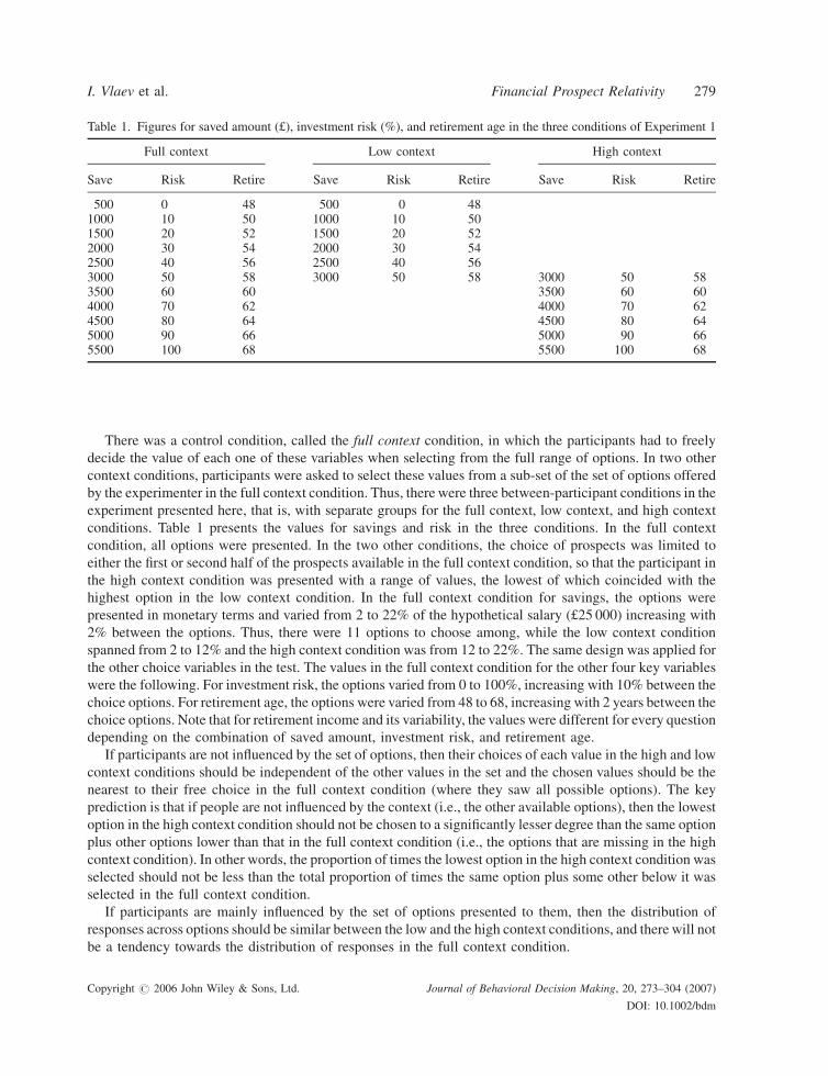
There was a control condition, called the full context condition, in which the participants had to freely
decide the value of each one of these variables when selecting from the full range of options. In two other
context conditions, participants were asked to select these values from a sub-set of the set of options offered
by the experimenter in the full context condition. Thus, there were three between-participant conditions in the
experiment presented here, that is, with separate groups for the full context, low context, and high context
conditions. Table 1 presents the values for savings and risk in the three conditions. In the full context
condition, all options were presented. In the two other conditions, the choice of prospects was limited to
either the first or second half of the prospects available in the full context condition, so that the participant in
the high context condition was presented with a range of values, the lowest of which coincided with the
highest option in the low context condition. In the full context condition for savings, the options were
presented in monetary terms and varied from 2 to 22% of the hypothetical salary (£25 000) increasing with
2% between the options. Thus, there were 11 options to choose among, while the low context condition
spanned from 2 to 12% and the high context condition was from 12 to 22%. The same design was applied for
the other choice variables in the test. The values in the full context condition for the other four key variables
were the following. For investment risk, the options varied from 0 to 100%, increasing with 10% between the
choice options. For retirement age, the options were varied from 48 to 68, increasing with 2 years between the
choice options. Note that for retirement income and its variability, the values were different for every question
depending on the combination of saved amount, investment risk, and retirement age.
If participants are not influenced by the set of options, then their choices of each value in the high and low
context conditions should be independent of the other values in the set and the chosen values should be the
nearest to their free choice in the full context condition (where they saw all possible options). The key
prediction is that if people are not influenced by the context (i.e., the other available options), then the lowest
option in the high context condition should not be chosen to a significantly lesser degree than the same option
plus other options lower than that in the full context condition (i.e., the options that are missing in the high
context condition). In other words, the proportion of times the lowest option in the high context condition was
selected should not be less than the total proportion of times the same option plus some other below it was
selected in the full context condition.
If participants are mainly influenced by the set of options presented to them, then the distribution of
responses across options should be similar between the low and the high context conditions, and there will not
be a tendency towards the distribution of responses in the full context condition.
Table 1. Figures for saved amount (£), investment risk (%), and retirement age in the three conditions of Experiment 1
Full context Low context High context
Save Risk Retire Save Risk Retire Save Risk Retire
500 0 48 500 0 481000 10 50 1000 10 501500 20 52 1500 20 522000 30 54 2000 30 542500 40 56 2500 40 563000 50 58 3000 50 58 3000 50 583500 60 60 3500 60 604000 70 62 4000 70 624500 80 64 4500 80 645000 90 66 5000 90 665500 100 68 5500 100 68
Copyright # 2006 John Wiley & Sons, Ltd. Journal of Behavioral Decision Making, 20, 273–304 (2007)
DOI: 10.1002/bdm
I. Vlaev et al. Financial Prospect Relativity 279
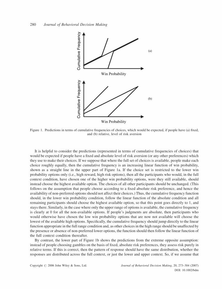
It is helpful to consider the predictions (represented in terms of cumulative frequencies of choices) that
would be expected if people have a fixed and absolute level of risk aversion (or any other preferences) which
they use to make their choices. If we suppose that where the full set of choices is available, people make each
choice roughly equally, then the cumulative frequency is an increasing linear function of win probability,
shown as a straight line in the upper part of Figure 1a. If the choice set is restricted to the lower win
probability options only (i.e., high reward, high risk options), then all the participants who would, in the full
context condition, have chosen one of the higher win probability options, were they still available, should
instead choose the highest available option. The choices of all other participants should be unchanged. (This
follows on the assumption that people choose according to a fixed absolute risk preference, and hence the
availability of non-preferred options should not affect their choices.) Thus, the cumulative frequency function
should, in the lower win probability condition, follow the linear function of the absolute condition and all
remaining participants should choose the highest available option, so that this point goes directly to 1, and
stays there. Similarly, in the case where only the upper range of options is available, the cumulative frequency
is clearly at 0 for all the non-available options. If people’s judgments are absolute, then participants who
would otherwise have chosen the low win probability options that are now not available will choose the
lowest of the available high options. Specifically, the cumulative frequency should jump directly to the linear
function appropriate in the full range condition and, as other choices in the high range should be unaffected by
the presence or absence of non-preferred lower options, the function should then follow the linear function of
the full context condition thereafter.
By contrast, the lower part of Figure 1b shows the predictions from the extreme opposite assumption:
instead of people choosing gambles on the basis of fixed, absolute risk preferences, they assess risk purely in
relative terms. If this is correct, then the pattern of response should have the same distribution, whether the
responses are distributed across the full context, or just the lower and upper context. So, if we assume that
Cum
ulat
ive
Fre
quen
cyWin Probability
Cum
ulat
ive
Fre
quen
cy
Win Probability
Win Probability
Win Probability
(a)
(b)
Figure 1. Predictions in terms of cumulative frequencies of choices, which would be expected, if people have (a) fixed,and (b) relative, level of risk aversion
Copyright # 2006 John Wiley & Sons, Ltd. Journal of Behavioral Decision Making, 20, 273–304 (2007)
DOI: 10.1002/bdm
280 Journal of Behavioral Decision Making
response is even in the full context condition (and hence that the cumulative probability function is linear),
then in the lower and upper contexts, the cumulative distribution should also be linear, but compressed over a
smaller number of choices items (i.e., with an increased slope).
MethodParticipants
Twelve participants took part in each condition of this study (i.e., 36 participants in total) recruited from the
University of Oxford student population via the experimental economics research groupmailing list of people
who have asked to be contacted. All were paid £5 for their participation.
Design
The questions were formulated as long-term saving/investment decision tasks related to retirement income
provision. The participants had to make decisions about five key variables. These variables were the saved
proportion of the current income, the risk of the investment expressed as the proportion invested in risky
assets,2 the retirement age, the desired income after retirement, and the preferred variability of this income
(participants were told that this variability is due to the uncertainty of economic conditions).
The experimental materials were designed as 10 independent hypothetical questions, in which we varied
each of the 5 key variables. Five of the questions focused only on savings while the other five questions
focused on risk and some questions showed how changing savings or risk would affect another variable or set
of variables. For example, one question showed how changing the investment risk can affect the projected
retirement income and its variability—with higher risk offering not only higher expected income on average,
but also wider spread of the possible values.3 Figure 2 presents this question in the full context condition, in
which the participants were asked to choose their preferred level of investment risk by selecting one of the
rows in the table (note that in this format, the key variable is in the first column of the table below, while the
other columns are showing the effects on the other variables like the minimum, average, and maximum
retirement income shown here):4
The high context condition was derived by deleting the lower five rows of the table for each question in the
full context condition and the low context condition was derived by deleting the higher five rows in the tables
in the full context condition (i.e., the same was done for each question). Therefore, in the full context
condition, the participants had to choose among 11 possible answer options for each question while in the
high and low context conditions, there were only 6 available answer options.
2There are various types of risky assets, like bonds and equities, for example, but in reality, these various investment vehicles differmainly in their risk-return characteristics.3In order to derive plausible figures for the various economic variables, we implemented a simple econometric model into a spreadsheetsimulator that calculates the likely impact of changes in each variable on the other four variables. For example, this model can derivewhatretirement income can be expected from certain savings, investment risk, and retirement age, or what are the possible potentialinvestment options that could lead to the preferred retirement income. Note also that all figures are in pounds and the participants knewthis.4Most of the questions showed the expected retirement income and its variability like in the example above. The possible variability of theretirement income was explained by referring to the 95% and respectively 5% confidence intervals of the income variability, that is,maximum and minimum possible values of the income, for which there is 5% chance to be more than the higher or less than the lowervalue, respectively. On each row of the table, these two values were placed on both sides of the average expected retirement income. Theconfidence intervals were expressed also in verbal terms using the words ‘‘very likely.’’ For example, the participants were informed thatit is very likely (95% chance) that their incomewill be below the higher value and above the lower value, and that these two values changedepending on the proportion of the investment in equities.
Copyright # 2006 John Wiley & Sons, Ltd. Journal of Behavioral Decision Making, 20, 273–304 (2007)
DOI: 10.1002/bdm
I. Vlaev et al. Financial Prospect Relativity 281

The 10 questions were presented in different orders in the various conditions. In Appendix A, there is a
detailed description of each question and its purpose (the questions are grouped by the key variable that
participants are asked to select savings or investment risk).
Procedure
Participants were given a booklet with 10 questions. They received written instructions explaining that the
purpose of the experiment was to answer a series of questions about savings and investment related to
retirement income provision, and that there were no right and wrong answers and they were free to choose
whatever most suits their preferences. It was explained that the choice options are predetermined as these are
the outcomes that can be realistically accomplished according to a standard economic model and that the task
was to choose the option nearest to the participant’s preferences. The participants were also informed that if
Assume that you will retire at 65 and decided to save 11% of your current salary (£2750) in order to provide for your retirement income. The following options offer different ranges of retirement income (in pounds) depending on the percentage of your savings allocated to shares (in the stock market) and you can see the effects on the expected average retirement income and its variability (minimum and maximum). Note that you are very likely (have 95% chance) to be between the minimum and maximum figures indicated in the table below. Please select one of the following options.
Invest Minimum Average Maximum
0 % 16,000 16,000 16,000
10 % 17,000 19,000 22,000
20 % 17,000 21,000 23,000
30 % 17,000 23,000 29,000
40 % 16,000 26,000 35,000
50 % 15,000 29,000 42,000
60 % 14,000 33,000 51,000
70 % 11,000 37,000 62,000
80 % 7,000 41,000 76,000
90 % 2,000 47,000 92,000
100 % 0 53,000 112,000
Figure 2. A question in the full range condition, in which the participants are asked to choose their preferred level ofinvestment risk
Copyright # 2006 John Wiley & Sons, Ltd. Journal of Behavioral Decision Making, 20, 273–304 (2007)
DOI: 10.1002/bdm
282 Journal of Behavioral Decision Making
they found all these options unsatisfactory, then they could indicate values outside these ranges. (We found
that none of the participants indicated such values.)
The questions and the answer options were presented in the sameway as the example question presented in
Figure 2. The participants had to choose one of the values in the first column of the table (which were either
savings or investment risk values) and they were provided with a separate answer sheet to write their answers.
Participants were informed that their answers did not need to be consistent between the questions, and that
they could freely change their preferences on each question and choose different savings and risk values.
ResultsParticipants took approximately 30 minutes to answer all questions. Note that although the questions related
to saving and to risk asked the participants to trade off different variables (e.g., savings versus retirement
income in one question, and savings versus risk in another question), we used the weighted average of the
answers of each participant across all five questions related to saving and all five questions related to risk in
order to derive the mean values for saving and risk in each condition. It is these averaged results that are
presented here. This was done because the results showed no difference (i.e., the general pattern was the
same) across the five questions for saving and risk, respectively.
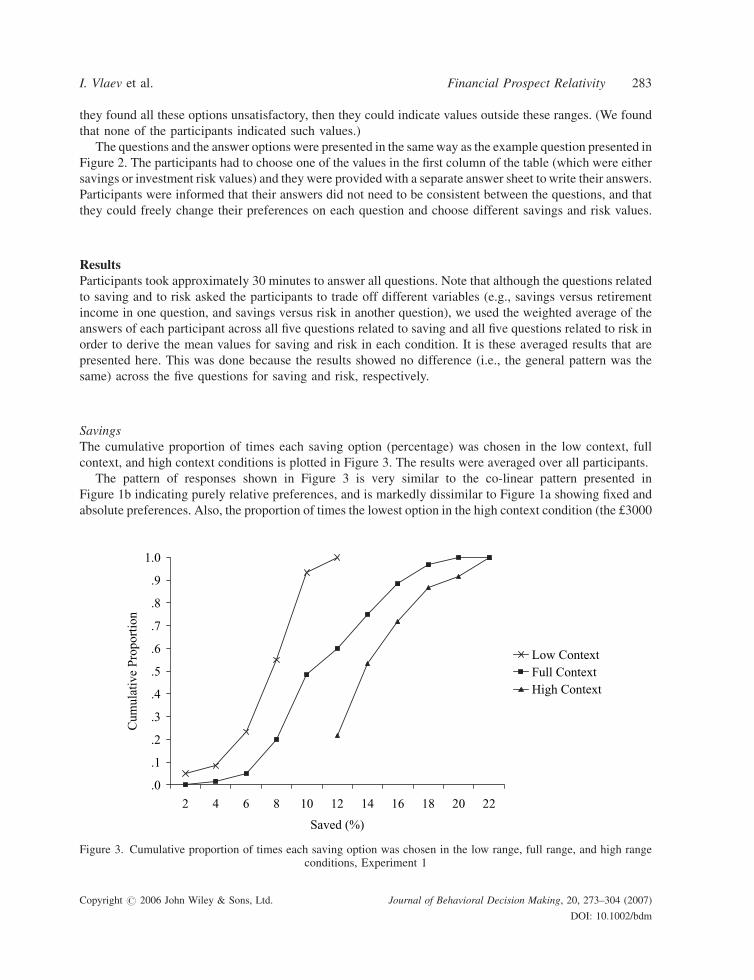
Savings
The cumulative proportion of times each saving option (percentage) was chosen in the low context, full
context, and high context conditions is plotted in Figure 3. The results were averaged over all participants.
The pattern of responses shown in Figure 3 is very similar to the co-linear pattern presented in
Figure 1b indicating purely relative preferences, and is markedly dissimilar to Figure 1a showing fixed and
absolute preferences. Also, the proportion of times the lowest option in the high context condition (the £3000
.0
.1
.2
.3
.4
.5
.6
.7
.8
.9
1.0
2 4 6 8 10 12 14 16 18 20 22
Saved (%)
noitroporPevitalu
muC
Low ContextFull ContextHigh Context
Figure 3. Cumulative proportion of times each saving option was chosen in the low range, full range, and high rangeconditions, Experiment 1
Copyright # 2006 John Wiley & Sons, Ltd. Journal of Behavioral Decision Making, 20, 273–304 (2007)
DOI: 10.1002/bdm
I. Vlaev et al. Financial Prospect Relativity 283
option) was selected was 0.22 and was significantly lower than 0.60, which is the proportion of times the same
option plus another option below it was selected in the full context condition, t(22)¼ 3.86, p¼ 0.001. This
result indicates that the context has significantly affected choices in the high context condition. The
proportion of times the highest option in the low context condition (again the £3000 option) was selected was
0.07 and this value was significantly lower than 0.52, which was the proportion of times the same option plus
some other option above in the full context condition was selected, t(22)¼ 3.76, p¼ 0.001. This result also
means that the hypothesis that participants’ choices were unaffected by context should be rejected. At the
same time, the greatest proportion of responses in the low range and high context conditions were
concentrated around the middle options of the whole context, which indicates that people seemed to prefer
moderate saving amounts.
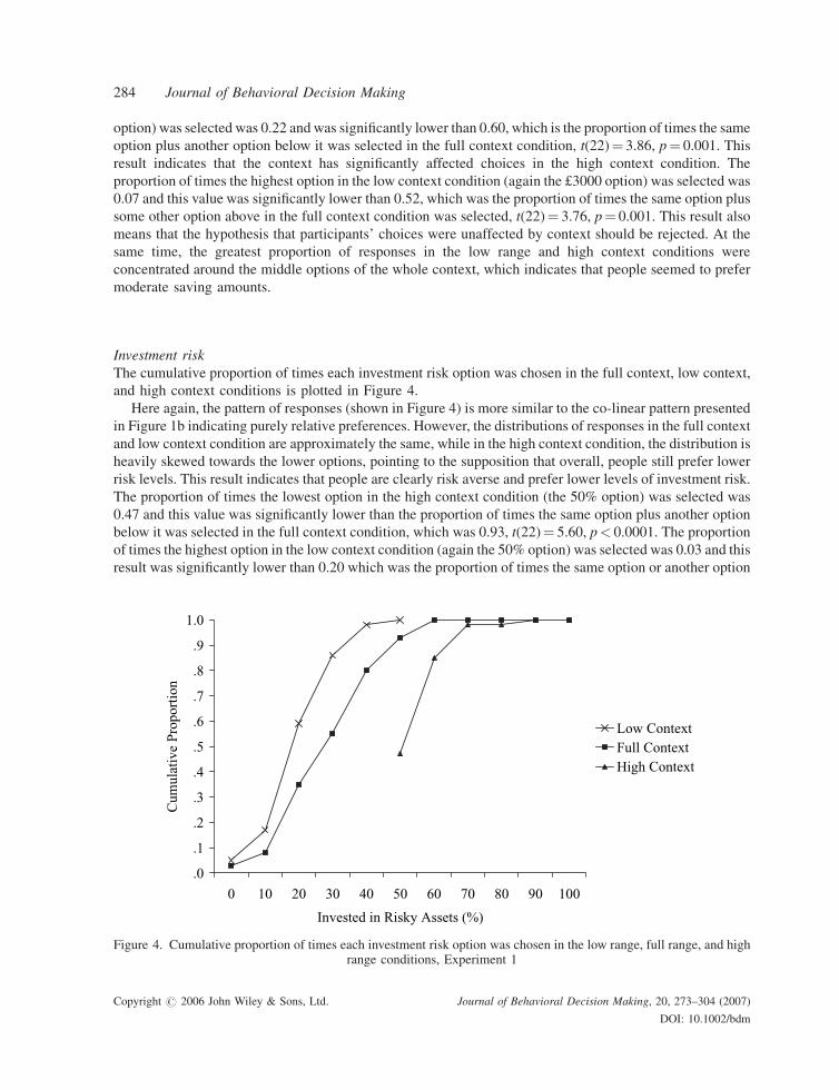
Investment risk
The cumulative proportion of times each investment risk option was chosen in the full context, low context,
and high context conditions is plotted in Figure 4.
Here again, the pattern of responses (shown in Figure 4) is more similar to the co-linear pattern presented
in Figure 1b indicating purely relative preferences. However, the distributions of responses in the full context
and low context condition are approximately the same, while in the high context condition, the distribution is
heavily skewed towards the lower options, pointing to the supposition that overall, people still prefer lower
risk levels. This result indicates that people are clearly risk averse and prefer lower levels of investment risk.
The proportion of times the lowest option in the high context condition (the 50% option) was selected was
0.47 and this value was significantly lower than the proportion of times the same option plus another option
below it was selected in the full context condition, which was 0.93, t(22)¼ 5.60, p< 0.0001. The proportion
of times the highest option in the low context condition (again the 50% option) was selected was 0.03 and this
result was significantly lower than 0.20 which was the proportion of times the same option or another option
.0
.1
.2
.3
.4
.5
.6
.7
.8
.9
1.0
0 10 20 30 40 50 60 70 80 90 100
Invested in Risky Assets (%)
noitroporPevitalu
muC
Low ContextFull ContextHigh Context
Figure 4. Cumulative proportion of times each investment risk option was chosen in the low range, full range, and highrange conditions, Experiment 1
Copyright # 2006 John Wiley & Sons, Ltd. Journal of Behavioral Decision Making, 20, 273–304 (2007)
DOI: 10.1002/bdm
284 Journal of Behavioral Decision Making
above it in the full context condition was selected, t(22)¼ 2.93, p¼ 0.008. These results show that context has
significantly biased people’s responses away from their likely choices in the full context condition.
DiscussionThe results clearly demonstrate that the choices were strongly influenced by the set of offered choice options.
The skewed results clearly show that there is a tendency towards certain preferred values for savings and risk.
This result suggests that people’s preferences are not completely malleable by the context and choices are not
absolutely relativistic and context dependent as the prospect relativity principle claims. This result might
arise, however, because the options are too far apart from each other. It is possible that if the options are
closely spaced, then people are more likely to be indifferent between them, and then the responses would be
less skewed and the relativity effect will arise. We conducted an additional experiment investigating the effect
of decreasing the spacing of the choice options and the results demonstrated that halving the spacing of the
options did not make the responses more evenly distributed and the effects of the choice set were the same as
in Experiment 1.
In Experiment 1, the ranks and the range of the choice options were manipulated at the same time when
comparing the high and low context condition versus the full context condition, which implies that the effects
could be due to either ranks or ranges [here, we mean range and rank as postulated by range–frequency theory
(Parducci, 1974)]. In other words, frequency values and range values as calculated strictly on the stimuli
presented are completely confounded. Thus, it does not make sense to claim that the effects of Experiment 1
are due to range rather than rank. However, the context effect can be observed even if we compare only the
low context and the high context condition, where all the corresponding options have the same rank and then
the context effects would appear even stronger. For example, if the majority of choices in the low context
condition are below the highest option, then in order to demonstrate context effects, we just need to show that
the total proportion of responses below the highest option in the low context is significantly higher than the
proportion of choices of the lowest option in the high context. This is evident from Figures 1 and 2. These
comparisons suggest the possibility that the results are not mainly due to rank effects.
Yet another alternative explanation of Experiment 1 could be that when participants are repeatedly
presented with trials containing too-high or too-low options, they learn to readjust their judgments to fit their
responses within the alternatives given (the same point was raised also by Stewart et al., 2003). In order to rule
out this alternative explanation, we conducted an additional experiment using a within-participants design, in
which each participant was presented with both high context and low context conditions (following Stewart
et al.). This design was supposed to test whether the participants could learn to adjust their judgments up or
down to fit into the response scale, which would also cause the observed effect of the choice set. Thus, these
effects should have disappeared when the participants were presented with both low and high contexts.
However, the pattern of results demonstrated in Experiment 1 was replicated, which suggests that the effect
was caused only by the options available on every trial (the data from this study are available on request).
In summary, the prospect relativity effect appeared when people were faced with familiar (most likely
previously experienced) situations, including saving, consumption, pension plans, and investment in the
capital markets (at least the media provide enough information on the last issue). It seems, however, that
people might have also developed some more stable preferences for risk, although their responses were still
malleable to context effects. In other words, the results showed that people were more context sensitive when
theymade decisions about savings, which implies that theymight not have a clear idea howmuch they need to
consume and save, respectively. This is a plausible conclusion as all participants in our experiments were
students who do not earn real income and therefore, are unlikely to have stable preferences concerning
consumption-savings ratios (in our hypothetical scenarios we just asked them to imagine that they earn
£25 000 per year).
Copyright # 2006 John Wiley & Sons, Ltd. Journal of Behavioral Decision Making, 20, 273–304 (2007)
DOI: 10.1002/bdm
I. Vlaev et al. Financial Prospect Relativity 285
EXPERIMENT 2
Experiment 1 demonstrated the significant effects of the set of offered values on risky choices, which suggests
that choice options are judged relative to each other when reaching a decision. There is substantial evidence
in the literature on perceptual judgment and also on risky decision-making that the skew of the distribution of
stimuli (i.e., their rank order) also affects the responses: stimuli with higher rank in the distribution (absolute
values held constant) are judged to have higher subjective values (e.g., Birnbaum, 1992; Brown, Gardner,
Oswald, & Qian, 2003; Janiszewski & Lichtenstein, 1999; Parducci, 1965, 1974). Recall that Birnbaum has
already demonstrated that when the options offered as certainty equivalents for simple prospects are
positively skewed and hence most values are small, then prospects are undervalued, while when the options
are negatively skewed and most values are large, then the prospects seem to be overvalued.
In order to investigate these effects on saving and investment decisions, we manipulated the skew of the
distribution of values so that in one condition, the distribution of options was positively skewed and in another
condition, the distribution of options was negatively skewed. There was one target option common to both
conditions, which had a higher rank in the positively skewed condition and a low rank in the negatively
skewed condition. Experiment 1 demonstrated a tendency for people to prefer lower risk options, and in order
to account (and control) for this tendency, we selected the common option to be equal to the natural mean in
the full context condition in Experiment 1 (i.e., the value that on average was most preferred by the
participants). So in this case, if there is a difference between the two groups in the proportion of times this
option was selected, then it is unlikely to be due to the fact that people prefer lower investment risk. The
preferred value for the saving questions was estimated to be 12% and 30% for the investment risk questions.
Therefore, we expected these two options to be perceived as lower values when they had a lower rank, which
could motivate people to select them more often compared to the condition in which they had a higher rank.
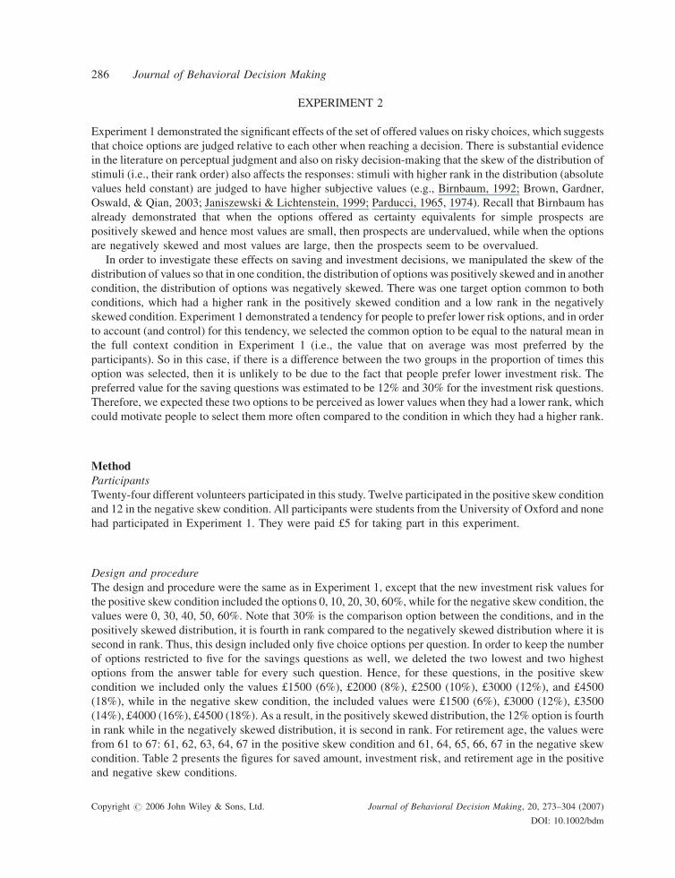
MethodParticipants
Twenty-four different volunteers participated in this study. Twelve participated in the positive skew condition
and 12 in the negative skew condition. All participants were students from the University of Oxford and none
had participated in Experiment 1. They were paid £5 for taking part in this experiment.
Design and procedure
The design and procedure were the same as in Experiment 1, except that the new investment risk values for
the positive skew condition included the options 0, 10, 20, 30, 60%, while for the negative skew condition, the
values were 0, 30, 40, 50, 60%. Note that 30% is the comparison option between the conditions, and in the
positively skewed distribution, it is fourth in rank compared to the negatively skewed distribution where it is
second in rank. Thus, this design included only five choice options per question. In order to keep the number
of options restricted to five for the savings questions as well, we deleted the two lowest and two highest
options from the answer table for every such question. Hence, for these questions, in the positive skew
condition we included only the values £1500 (6%), £2000 (8%), £2500 (10%), £3000 (12%), and £4500
(18%), while in the negative skew condition, the included values were £1500 (6%), £3000 (12%), £3500
(14%), £4000 (16%), £4500 (18%). As a result, in the positively skewed distribution, the 12% option is fourth
in rank while in the negatively skewed distribution, it is second in rank. For retirement age, the values were
from 61 to 67: 61, 62, 63, 64, 67 in the positive skew condition and 61, 64, 65, 66, 67 in the negative skew
condition. Table 2 presents the figures for saved amount, investment risk, and retirement age in the positive
and negative skew conditions.
Copyright # 2006 John Wiley & Sons, Ltd. Journal of Behavioral Decision Making, 20, 273–304 (2007)
DOI: 10.1002/bdm
286 Journal of Behavioral Decision Making
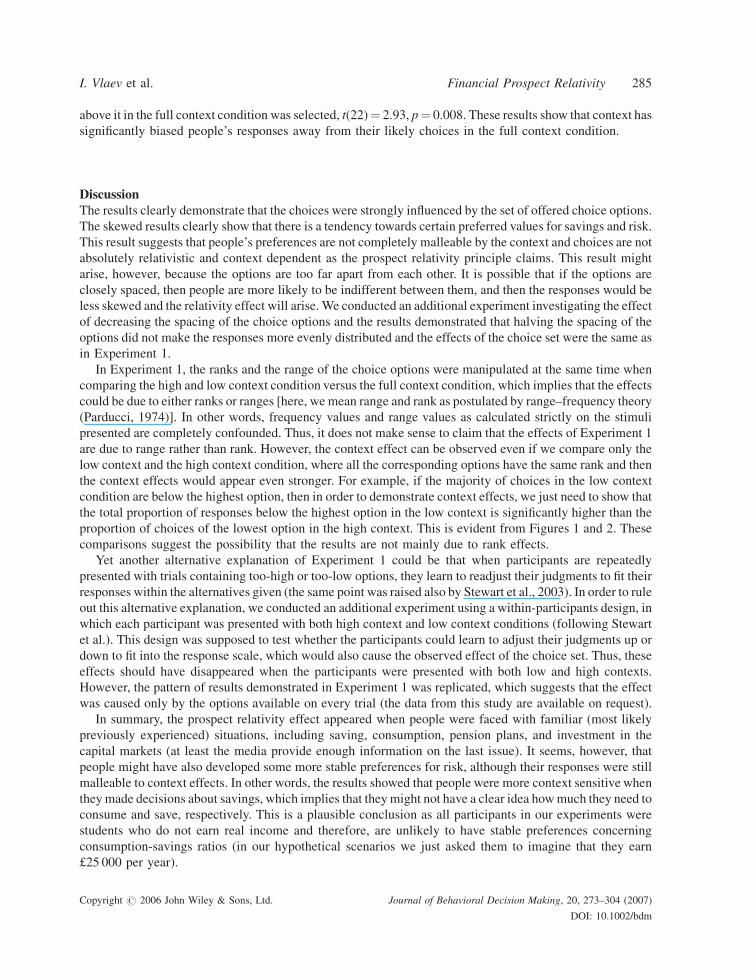
ResultsSavings
The proportion of times each saving option was chosen in the positive skew and negative skew conditions is
plotted in Figure 5. The error bars represent the standard error of the mean.
The distribution of responses in each condition seems to be skewed towards the central option, similar to
the full context condition in Experiment 1. There was no significant difference between the proportion of
times the option £3000 (12%) was selected in the two groups (0.33 in the negative skew condition versus
0.30 in the positive skew condition), t(22)¼�0.28, p¼ 0.780, which means that the rank order of options did
not have an effect on the common saving option. Note that we expected that the 12% option would be
perceived as less attractive in the positively skewed distribution, where it was fourth in rank compared to the
negatively skewed distribution, where it was second in rank. The results did not support this prediction.
Note also that although this can be interpreted as a lack of context effect on the perception of a particular
item, there is still a huge context effect in terms of the cumulative analysis we presented in Experiment 1. In
the negatively skewed context, nearly all participants saved 12% or more, while in the positively skewed
context, only around 75% did so. Such a difference indicates a strong difference in evaluations and choices
related to amount of savings as a function of context.
Table 2. Figures for saved amount (£), investment risk (%), and retirement age in the two conditions of Experiment 2
Low context High context
Save Risk Retire Save Risk Retire
1500 0 61 1500 0 612000 10 622500 20 633000 30 64 3000 30 64
3500 40 654000 50 66
4500 60 67 4500 60 67
.0
.1
.2
.3
.4
.5
6 8 10 12 14 16 18
Saved (%)
Prop
ortio
n
Positive Skew
Negative Skew
Figure 5. Proportion of times each saving option was chosen in the positive skew and negative skew conditions,Experiment 2. (Error bars are standard error of the mean)
Copyright # 2006 John Wiley & Sons, Ltd. Journal of Behavioral Decision Making, 20, 273–304 (2007)
DOI: 10.1002/bdm
I. Vlaev et al. Financial Prospect Relativity 287
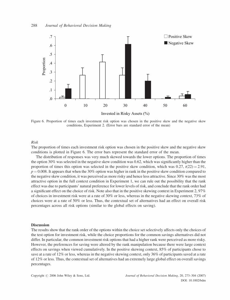
Risk
The proportion of times each investment risk option was chosen in the positive skew and the negative skew
conditions is plotted in Figure 6. The error bars represent the standard error of the mean.
The distribution of responses was very much skewed towards the lower options. The proportion of times
the option 30% was selected in the negative skew condition was 0.62, which was significantly higher than the
proportion of times this option was selected in the positive skew condition, which was 0.27, t(22)¼ 2.91,
p¼ 0.008. It appears that when the 30% option was higher in rank in the positive skew condition compared to
the negative skew condition, it was perceived as more risky and hence less attractive. Since 30%was the most
attractive option in the full context condition in Experiment 1, we can rule out the possibility that the rank
effect was due to participants’ natural preference for lower levels of risk, and conclude that the rank order had
a significant effect on the choice of risk. Note also that in the positive skewing context in Experiment 2, 97%
of choices in investment risk were at a rate of 30% or less, whereas in the negative skewing context, 73% of
choices were at a rate of 50% or less. Thus, the contextual set of alternatives had an effect on overall risk
percentages across all risk options (similar to the global effects on saving).
DiscussionThe results show that the rank order of the options within the choice set selectively affects only the choices of
the test option for investment risk, while the choice proportions for the common savings alternatives did not
differ. In particular, the common investment risk options that had a higher rank were perceived as more risky.
However, the preferences for saving were altered by the rank manipulation because there were large context
effects on savings when viewed cumulatively. In the positive skewing context, 85% of participants chose to
save at a rate of 12% or less, whereas in the negative skewing context, only 36% of participants saved at a rate
of 12% or less. Thus, the contextual set of alternatives had an extremely large global effect on overall savings
percentages.
.0
.1
.2
.3
.4
.5
.6
.7
0 10 20 30 40 50 60
Invested in Risky Assets (%)
Positive Skew
Negative SkewPr
opor
tion
Figure 6. Proportion of times each investment risk option was chosen in the positive skew and the negative skewconditions, Experiment 2. (Error bars are standard error of the mean)
Copyright # 2006 John Wiley & Sons, Ltd. Journal of Behavioral Decision Making, 20, 273–304 (2007)
DOI: 10.1002/bdm
288 Journal of Behavioral Decision Making
An interesting difference is that the effect of the choice set was stronger for the savings than for the
risk-related decisions in Experiment 1, while the reverse result was evident for the effects of the skew on the
target common option in Experiment 2, where the context effect on this option was stronger for the risk than
for the saving decisions. One possible interpretation of this particular result is that there might be different
weighting on the range and rank factors for the different dimensions of judgment, which was originally
proposed by the range–frequency theory (Parducci, 1965, 1974). Thus, there is a parameter that specifies the
relative contributions of rank and range, and it is possible that for certain attributes, the contributions of range
and rank are exclusively weighted towards one of these two factors (by setting the weight of the other factor
equal to 0). Therefore, it is possible that in Experiment 2, there has been differential weighting of the impact
of rank (skew) on the judgments related to saving and risk. One possible interpretation is that rank is more
strongly affecting the choices of risk (and hence no effect on the common test option). However, the large
context effects on savings when viewed cumulatively suggest also the interpretation that there is no local
effect on the particular item (as we expected), but there is a global effect across the whole range of options. In
order to further test the validity of these ad hoc explanations, we conducted Experiment 3.
EXPERIMENT 3
In order to test the hypothesis that savings and risk receive different weights, we next further manipulated the
skew of the distribution of values. One possible reason for the lack of an affect upon savings in Experiment 2
is that the range of presented values was too narrow and the 12% saving option was only fourth in rank. This
ranking might not have been enough to make the participants rate this option as high (although it worked for
risk, but this could simply mean that people are more sensitive to changes in risk and variability). Thus, a
direct way to test the relative weighting of the rank is simply to conduct an experiment testing whether one or
another dimension of judgment is more or less affected by manipulation of the rank of the test options.
In this experiment, the 12% saving option was sixth in rank. The range of values spanned from 0 to 100%
for risk and from 2 to 22% for savings (as in the full context condition in Experiment 1). The comparison
options between the positive and negative skew conditions were again the 12% savings option and this time,
the 50% risk option (because the test options should be positioned in the middle of the range of presented
values). If the effects of the choice set were the same as in Experiment 2, that is, no effect on the 12% saving
option, while the 50% risk option was again significantly more attractive in the negatively skewed condition
(when it was second in rank), then this is plausible evidence that the rank does not have a significant local
effect on individual common items.
In summary, for the savings options in the positively skewed distribution, the offered values were: 2, 4, 6,
8, 10, 12, 22%; while in the negatively skewed distribution, the offered values were: 2, 12, 14, 16, 18, 20,
22%. In the positively skewed condition, the option 12% has a higher rank by being sixth in the rank order of
options, compared to the same option in the negatively skewed condition. Thus, we assumed that if we used a
wider range of possible values, this would further corroborate the results in Experiment 2.
The same principles applied in the design of the investment risk options. Thus the condition with the
positive skew contained the values 0, 10, 20, 30, 40, 50, 100%; while the negative skew condition included the
options 0, 50, 60, 70, 80, 90, 100%. Here, the key comparison between the two groups was the option 50%,
which had different rank in the two conditions: in the positive skew, it was sixth in rank, while in the negative
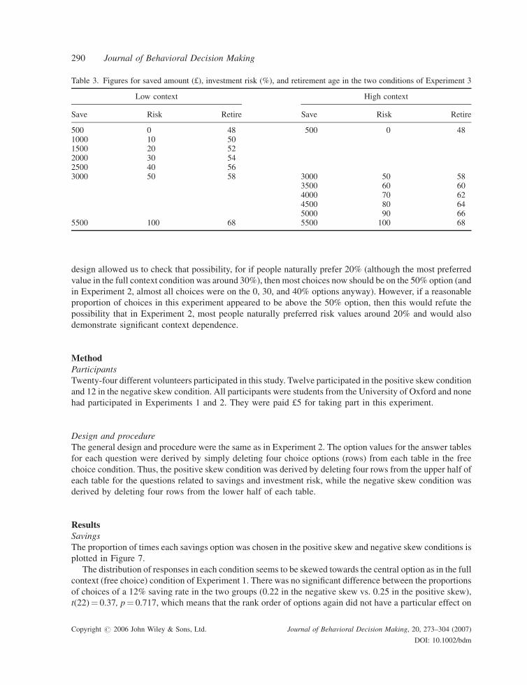
skew, it was second in rank. Table 3 presents the figures for saved amount, investment risk, and retirement age
in the positive and negative skew conditions.
This design of the risk options can also help us to resolve an interpretation problem with the results for risk
in Experiment 2. Specifically, it allows us to see if the very high preference for the 30% option in the negative
skew in Experiment 2 could have arisen from an ideal (natural) risk preference of around 20% amongst most
participants (and hence, given the limited choice options, they should choose the 30% option). The current
Copyright # 2006 John Wiley & Sons, Ltd. Journal of Behavioral Decision Making, 20, 273–304 (2007)
DOI: 10.1002/bdm
I. Vlaev et al. Financial Prospect Relativity 289
design allowed us to check that possibility, for if people naturally prefer 20% (although the most preferred
value in the full context condition was around 30%), then most choices now should be on the 50% option (and
in Experiment 2, almost all choices were on the 0, 30, and 40% options anyway). However, if a reasonable
proportion of choices in this experiment appeared to be above the 50% option, then this would refute the
possibility that in Experiment 2, most people naturally preferred risk values around 20% and would also
demonstrate significant context dependence.
MethodParticipants
Twenty-four different volunteers participated in this study. Twelve participated in the positive skew condition
and 12 in the negative skew condition. All participants were students from the University of Oxford and none
had participated in Experiments 1 and 2. They were paid £5 for taking part in this experiment.
Design and procedure
The general design and procedure were the same as in Experiment 2. The option values for the answer tables
for each question were derived by simply deleting four choice options (rows) from each table in the free
choice condition. Thus, the positive skew condition was derived by deleting four rows from the upper half of
each table for the questions related to savings and investment risk, while the negative skew condition was
derived by deleting four rows from the lower half of each table.
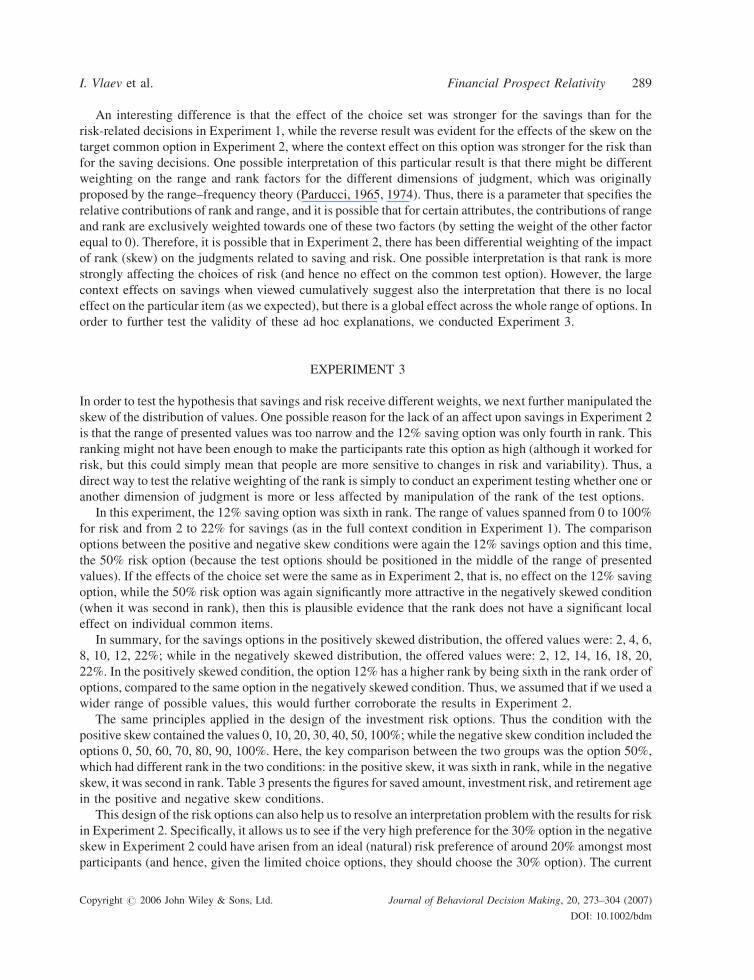
ResultsSavings
The proportion of times each savings option was chosen in the positive skew and negative skew conditions is
plotted in Figure 7.
The distribution of responses in each condition seems to be skewed towards the central option as in the full
context (free choice) condition of Experiment 1. There was no significant difference between the proportions
of choices of a 12% saving rate in the two groups (0.22 in the negative skew vs. 0.25 in the positive skew),
t(22)¼ 0.37, p¼ 0.717, which means that the rank order of options again did not have a particular effect on
Table 3. Figures for saved amount (£), investment risk (%), and retirement age in the two conditions of Experiment 3
Low context High context
Save Risk Retire Save Risk Retire
500 0 48 500 0 481000 10 501500 20 522000 30 542500 40 563000 50 58 3000 50 58
3500 60 604000 70 624500 80 645000 90 66
5500 100 68 5500 100 68
Copyright # 2006 John Wiley & Sons, Ltd. Journal of Behavioral Decision Making, 20, 273–304 (2007)
DOI: 10.1002/bdm
290 Journal of Behavioral Decision Making
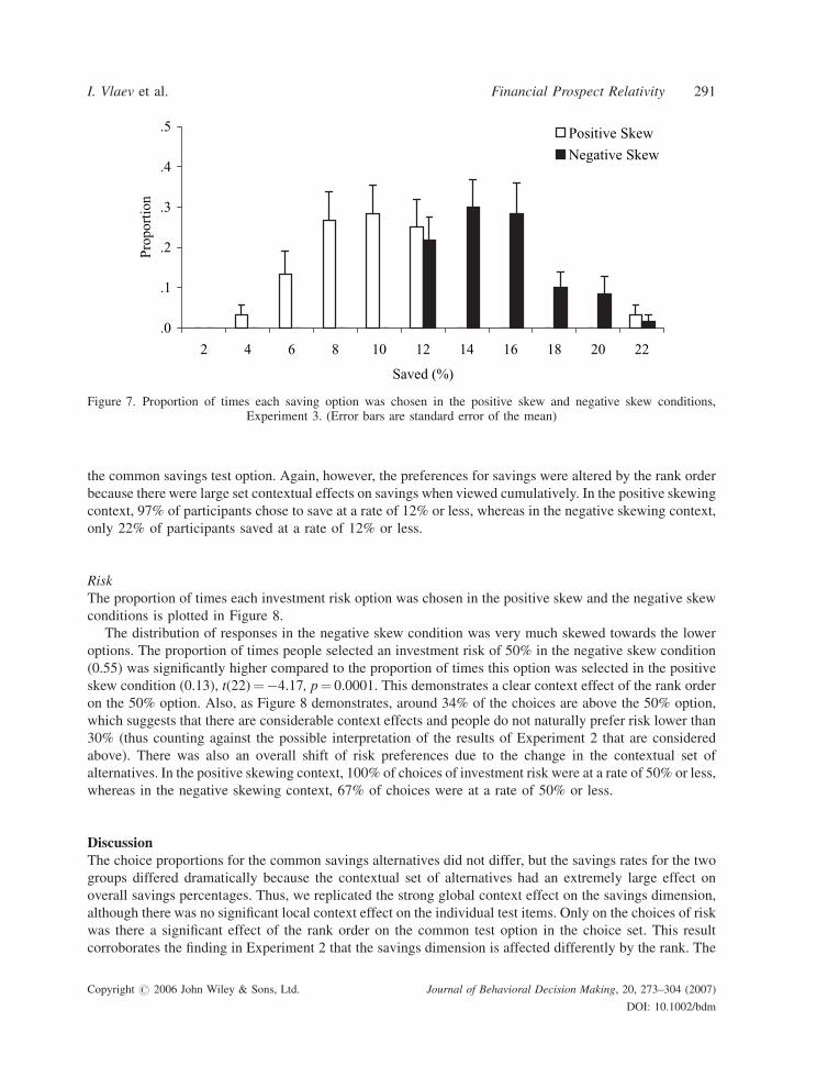
the common savings test option. Again, however, the preferences for savings were altered by the rank order
because there were large set contextual effects on savings when viewed cumulatively. In the positive skewing
context, 97% of participants chose to save at a rate of 12% or less, whereas in the negative skewing context,
only 22% of participants saved at a rate of 12% or less.
Risk
The proportion of times each investment risk option was chosen in the positive skew and the negative skew
conditions is plotted in Figure 8.
The distribution of responses in the negative skew condition was very much skewed towards the lower
options. The proportion of times people selected an investment risk of 50% in the negative skew condition
(0.55) was significantly higher compared to the proportion of times this option was selected in the positive
skew condition (0.13), t(22)¼�4.17, p¼ 0.0001. This demonstrates a clear context effect of the rank order
on the 50% option. Also, as Figure 8 demonstrates, around 34% of the choices are above the 50% option,
which suggests that there are considerable context effects and people do not naturally prefer risk lower than
30% (thus counting against the possible interpretation of the results of Experiment 2 that are considered
above). There was also an overall shift of risk preferences due to the change in the contextual set of
alternatives. In the positive skewing context, 100% of choices of investment risk were at a rate of 50% or less,
whereas in the negative skewing context, 67% of choices were at a rate of 50% or less.
DiscussionThe choice proportions for the common savings alternatives did not differ, but the savings rates for the two
groups differed dramatically because the contextual set of alternatives had an extremely large effect on
overall savings percentages. Thus, we replicated the strong global context effect on the savings dimension,
although there was no significant local context effect on the individual test items. Only on the choices of risk
was there a significant effect of the rank order on the common test option in the choice set. This result
corroborates the finding in Experiment 2 that the savings dimension is affected differently by the rank. The
.0
.1
.2
.3
.4
.5
2 4 6 8 10 12 14 16 18 20 22
Saved (%)
noitroporPPositive Skew
Negative Skew
Figure 7. Proportion of times each saving option was chosen in the positive skew and negative skew conditions,Experiment 3. (Error bars are standard error of the mean)
Copyright # 2006 John Wiley & Sons, Ltd. Journal of Behavioral Decision Making, 20, 273–304 (2007)
DOI: 10.1002/bdm
I. Vlaev et al. Financial Prospect Relativity 291
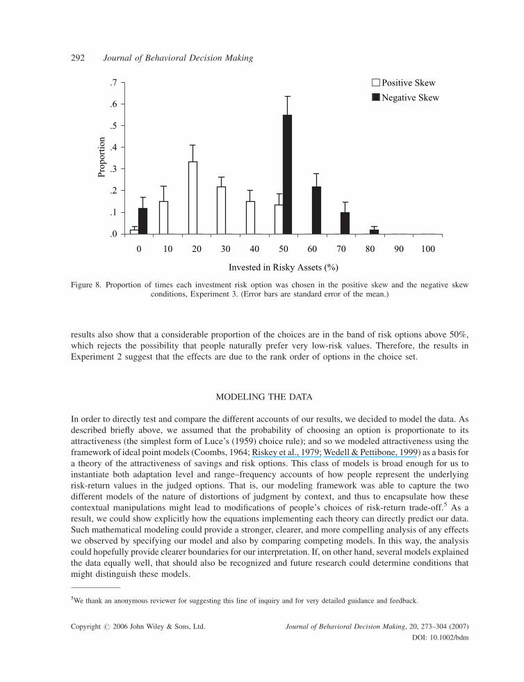
results also show that a considerable proportion of the choices are in the band of risk options above 50%,
which rejects the possibility that people naturally prefer very low-risk values. Therefore, the results in
Experiment 2 suggest that the effects are due to the rank order of options in the choice set.
MODELING THE DATA
In order to directly test and compare the different accounts of our results, we decided to model the data. As
described briefly above, we assumed that the probability of choosing an option is proportionate to its
attractiveness (the simplest form of Luce’s (1959) choice rule); and so we modeled attractiveness using the
framework of ideal point models (Coombs, 1964; Riskey et al., 1979;Wedell & Pettibone, 1999) as a basis for
a theory of the attractiveness of savings and risk options. This class of models is broad enough for us to
instantiate both adaptation level and range–frequency accounts of how people represent the underlying
risk-return values in the judged options. That is, our modeling framework was able to capture the two
different models of the nature of distortions of judgment by context, and thus to encapsulate how these
contextual manipulations might lead to modifications of people’s choices of risk-return trade-off.5 As a
result, we could show explicitly how the equations implementing each theory can directly predict our data.
Such mathematical modeling could provide a stronger, clearer, and more compelling analysis of any effects
we observed by specifying our model and also by comparing competing models. In this way, the analysis
could hopefully provide clearer boundaries for our interpretation. If, on other hand, several models explained
the data equally well, that should also be recognized and future research could determine conditions that
might distinguish these models.
.0
.1
.2
.3
.4
.5
.6
.7
Prop
ortio
n
0 10 20 30 40 50 60 70 80 90 100
Invested in Risky Assets (%)
Positive Skew
Negative Skew
Figure 8. Proportion of times each investment risk option was chosen in the positive skew and the negative skewconditions, Experiment 3. (Error bars are standard error of the mean.)
5We thank an anonymous reviewer for suggesting this line of inquiry and for very detailed guidance and feedback.
Copyright # 2006 John Wiley & Sons, Ltd. Journal of Behavioral Decision Making, 20, 273–304 (2007)
DOI: 10.1002/bdm
292 Journal of Behavioral Decision Making
The hope, then, was that this framework would allow us to see how far modification of an ideal point
constructed by the current set could possibly account for the choice-set effects that were observed in
Experiments 1–3—whether from an adaptation level theory or a range–frequency theory perspective. For
example, having such a constructed ideal point could possibly account for the choice set effects in
Experiment 1, where the mean was relatively high in the high context, average in the full context, and low in
the low context; and also for skew effects as in Experiment 2, where the mean was higher in the negative skew
condition, in which the comparison options were above the mean, while in the positive skew condition, the
key options were below the mean. The position and the malleability of the ideal could also possibly reveal
why there was no rank effect on the comparison options (12%) for savings in Experiment 3. If we assume that
the ideal has not changed between the context conditions and is fixed on the comparison option, this would
imply that there would be no difference between the comparison options across context conditions.
There are several ways that a modeling framework for data of this kind may be constructed. One is given in
a recent paper by Cooke, Janiszewski, Cunha, Nasco, and De Wilde (2004). These authors show one way to
combine range–frequency scales to determine preference judgments. Another approach is presented by
Wedell and Pettibone (1999), who show that a Gaussian ideal point model can use the range–frequency scale
or the stimulus scale with shifting adaptation levels. We chose this latter method to do a data fit, as it allows us
to compare with ease the two main theoretical contenders, range–frequency theory and adaptation level
theory.
Following the simplest form of Luce’s choice rule, that the probability of choosing an option i, in context k,
is proportional to its attractiveness, our basic assumption is:
PrðChooseikÞ ¼ AttractikP
j
Attractjk(1)
We modeled a single-peaked preference for savings and risk with a Gaussian similarity function of the
form:
Attractik ¼ aþ b � e�cðRepik�IdealkÞ2 (2)
where the attractiveness of stimulus i in context k is a rapidly decreasing function of the distance between
the subjective value, Repik, of stimulus i in context k (i.e., Rep denotes its representation on a putative internal
psychological scale) and the Ideal (i.e., ideal point or most preferred value on the particular dimension) in
context k. The b parameter of Equation 2 was not used, as it is just a multiplicative constant (determining the
height of the function when mapping it onto the stimulus scale) and the Luce rule is invariant under
multiplicative constants. The additive constant a was also dropped, as it is almost 0.0 for all the fits. In other
words, we fixed parameters a¼ 0 and b¼ l. The discriminability parameter c (determining the width or
narrowness of the rating function), the scale value, and the ideal point (Idealk), were allowed to differ with
context. Thus, the differences between contexts were captured by variation of these three parameters.
The range–frequency-based model assumes that the relevant magnitudes (here risk-return values) are not
represented in absolute terms, but according to the range–frequency theory. Ideal values are then estimated as
free parameters. More specifically, range–frequency theory uses the following equation:
Repik ¼ wRik þ ð1� wÞFik (3)
where Repik is the internal representation of stimulus i in context k. Rik is the range value and Fik is the
‘‘frequency’’ (or more accurately ‘‘rank’’) value of stimulus i in context k, while w represents the relative
Copyright # 2006 John Wiley & Sons, Ltd. Journal of Behavioral Decision Making, 20, 273–304 (2007)
DOI: 10.1002/bdm
I. Vlaev et al. Financial Prospect Relativity 293
weighting of range and frequency values. Range values are calculated by the following equation:
Rik ¼ Si �Mink
Maxk �Mink(4)
where Si is the objective scale value of the stimulus, and Mink and Maxk are scale values defining the
subjective range. Frequency values are calculated using the following equation:
Fik ¼ rankik � 1
Nk � 1(5)
where rankik is the rank in the stimulus context, and Nk is the total number of stimuli making up the
context.
In order to implement adaptation level theory as outlined by Helson (1964), we decided to fix the scale
value as equal to the stimulus value (i.e., assuming no subjective transformation, as in range–frequency
theory), that is, Repik¼ Si. We then let the ideals be determined by a version of adaptation level theory that
weights the mean of the stimulus series with a background value:
Idealk ¼ w�ðBackgroundÞ þ ð1� w�ÞS meank (6)
where Background is the adaptation level with which participants begin the experiment and S_meank is the
mean of the stimuli in context k; w� represents the relative weighting of the two. Thus, adaptation level is a
weighted average of a background value and the mean of the values experienced (Helson, 1964). This model
has three free parameters—c, w�, and the Background adaptation level.
MethodEquation 1 was used in the fitting procedure using a maximum likelihood fit to the proportion data. By fitting
the proportions directly rather than using conventional least squares fit to means, the maximum likelihood
procedure would yield more accurate estimates. As these are proportions, they must sum to 1.0 so that for six
data points (choice proportions) in a distribution (e.g., in the low context condition in Experiment 1), only five
are free to vary as the last one must equal one minus the sum of other proportions. This constraint is part of
Equation 1 and was reflected in the fitting procedure and degrees of freedom.
Our initial approach was to fit a single model to the data across the contextual conditions and free up
parameters if this provided a better fit. There was a baseline model with just two parameters, c, and Ideal,
which was compared to hierarchically nested models that allow the ideal point to vary with context or to have
a separate parameter c, for each context condition. Thus, for the savings results in Experiment 1, this meant
fitting the 23 data points (proportions) for full, low, and high context conditions (shown on Figure 3) with a
single equation. This was done by dummy coding the contextual conditions and then multiplying the dummy
codes by a unique parameter for each condition, (e.g., ideal—high, ideal—low, etc.) in order to fit that
parameter to that condition, whilst holding the other parameters of the model constant all conditions. Thus,
there is a loss of one degree of freedom for each distribution (i.e., condition) included in the fitting procedure.
For example, in fitting Experiment 1, we lose 3 degrees of freedom because there are three choice sets
(conditions) fitted simultaneously with the same set of parameters.
Using this hierarchical approach, we tested the need for the free parameters by looking at change in the
Akaike information criterion (AIC, which is a statistical model fit measure developed by Akaike (1974); see
also Burnham & Anderson, 2002; though see Pitt, Myung, & Zhang, 2002, for an alternative approach). It
quantifies the relative goodness-of-fit of various previously derived statistical models, given a sample of data.
It uses a rigorous framework of information analysis based on the concept of entropy. The driving idea behind
Copyright # 2006 John Wiley & Sons, Ltd. Journal of Behavioral Decision Making, 20, 273–304 (2007)
DOI: 10.1002/bdm
294 Journal of Behavioral Decision Making
the AIC is to examine the complexity of the model together with the goodness of its fit to the sample data, and
to then produce a measure which balances the two. Its formula is:
AIC ¼ 2k � 2 lnðLÞ (7)
where k is the number of parameters, and L is the maximum likelihood function. A model with many
parameters will provide a very good fit to the data, but will have fewer degrees of freedom and be of limited
utility. This balanced approach discourages overfitting (i.e., favoring parsimony and simplicity). The
preferred model is that with the lowest AIC value. The AIC methodology attempts to find the minimal model
that correctly explains the data, which can be contrasted with more traditional approaches to modeling, such
as starting from a null hypothesis. Variations of AIC include AICc, which is better than AIC when sample size
(the number of observations), n, is small (i.e., n/k<�40). The formula for AICc is:
AICc ¼ AICþ 2kðk þ 1Þn� k � 1
(8)
Since AICc converges to AIC as n gets large (the last term of the AICc approaches zero), it is
recommended to practically use AICc in any case (Burnham & Anderson, 2002, 2004).
There is one simple measure associated with the AIC, which can be used to compare models: the delta
AIC. It is easy to compute, as calculations remain the same regardless of whether the AIC or AICc is used,
and also has the advantage of being easy to interpret (another good measure is the more complicated Akaike
weight which we do not consider here). The delta AIC (Di), is a measure of each model relative to the best
model, and is calculated as
Delta AIC ¼ Di ¼ AICi �minAIC (9)
where AICi is the AIC value for model i, and minAIC is the AIC value of the best model. As a rule of
thumb, a Di< 2 suggests substantial evidence for the model, values between 3 and 7 indicate that the model
has considerably less support, whereas a Di> 10 indicates that the model is very unlikely (Burnham &
Anderson, 2002). Note that the AIC is not a hypothesis test, does not have an a-value, and does not use
notions of significance. Instead, the AIC focuses on the strength of evidence (i.e., Di), and gives a measure of
uncertainty for each model. We decided to compare the performance of the two models on the basis of AICc
as it provides a better balance between the complexity of the model and the goodness of its fit to the sample
data.
The method described above tests the more generic and important question of whether context effects in
Experiments 1–3 can be adequately described as a shift in ideal points along a single continuum, following
the basic assertion by Coombs in his portfolio theory (Coombs, 1969, 1975) that there is an ideal risk value. In
addition, this method could in principle allow us to test between models, such as the adaptation level model
and range–frequency valuation.
As we show in Equation 6, the adaptation level model is developed by simply substituting into Equation 2
the right side of Equation 6 for the Idealk parameter. Note this should be done under the constraint that the
parameters Background and w are held constant for individuals within an experiment so that any changes in
contextual shifts of ideals are attributed to differences in the means of the distributions. (The other parameters
merely set an intercept and a limit on the modulation of the ideal by the change in context.) Here, we
simultaneously fitted the model across contextual conditions and constrained the parameters across these
conditions. For example, to fit Experiment 1, we hold c, w�, and Background constant so that the 23
proportions (or frequencies, as we used the maximum likelihood fitting method) are fitted by 3 parameters.
This 3-parameter model allows weighting of the mean of the contextual series (via fitting w) and thus,
different ideal points can be predicted by the differences in means.
Copyright # 2006 John Wiley & Sons, Ltd. Journal of Behavioral Decision Making, 20, 273–304 (2007)
DOI: 10.1002/bdm
I. Vlaev et al. Financial Prospect Relativity 295
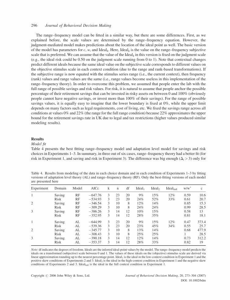
The range–frequency model can be fitted in a similar way, but there are some differences. First, as we
explained before, the scale values are determined by the range–frequency equation. However, the
judgment-mediated model makes predictions about the location of the ideal point as well. The basic version
of the model has parameters for c, w, and Idealk. Here, Idealk is the value on the range–frequency subjective
scale that is preferred. We can assume that the value of the Idealk in this version is fixed on the judgment scale
(e.g., the ideal risk could be 0.50 on the judgment scale running from 0 to 1). Note that contextual changes
predict different ideals because the same ideal value on the subjective scale corresponds to different values on
the objective stimulus scale in each context condition (due to the range and rank-based transformations). If
the subjective range is now equated with the stimulus series range (i.e., the current context), then frequency
(rank) values and range values are the same (i.e., range values become useless in this implementation of the
range–frequency theory). In order to overcome this problem, we assumed that people enter the lab with the
full range of possible savings and risk values. For risk, it is natural to assume that people anchor the possible
percentage of their retirement savings that can be invested in risky assets on between 0 and 100% (obviously
people cannot have negative savings, or invest more than 100% of their savings). For the range of possible
savings values, it is equally easy to imagine that the lower boundary is fixed at 0%, while the upper limit
depends on many factors such as legal requirements, cost of living, etc. We fixed the savings range across all
conditions at values 0% and 22% (the range for the full range condition) because 22% approximates the upper
bound for the retirement savings rate in UK due to legal and tax restrictions (higher values produced similar
modeling results).
ResultsModel fit
Table 4 presents the best fitting range–frequency model and adaptation level model for savings and risk
choices in Experiments 1–3. In summary, in three out of six cases, range–frequency theory had a better fit (for
risk in Experiment 1, and saving and risk in Experiment 3). The difference was big enough (Di> 3) only for
Table 4. Results from modeling of the data in each choice domain and in each condition of Experiments 1–3 by fittingversions of adaptation level theory (AL) and range–frequency theory (RF). Only the best-fitting versions of each modelare presented here
Experiment Domain Model AICc k n df Ideal1 Ideal2 Idealfull w/w� c
1 Saving RF �647.76 3 23 20 9% 15% 12% 0.59 10.6Risk RF �534.93 3 23 20 24% 52% 33% 0.61 20.7
2 Saving RF �346.54 3 10 8 12% 14% 0.85 15.3Risk RF �309.29 3 10 8 24% 24% 0.99 28.5
3 Saving RF �386.26 3 14 12 10% 15% 0.58 13Risk RF �352.95 3 14 12 28% 35% 0.81 18.1
1 Saving AL �644.99 3 23 20 9% 15% 12% 0.47 373.4Risk AL �539.36 3 23 20 23% 45% 34% 0.55 25.7
2 Saving AL �345.77 3 10 8 13% 14% 0.68 477.9Risk AL �308.43 3 10 8 25% 25% 1 28.5
3 Saving AL �390.18 3 14 12 12% 14% 0.73 312.2Risk AL �353.37 3 14 12 28% 33% 0.82 19
Note: df indicates the degrees of freedom. Ideals are the inferred ideal-point values by the model. The range–frequencymodel predicts theideals on a transformed (subjective) scale between 0 and 1. The values of these ideals on the (objective) stimulus scale are derived vialinear approximation rounding up to the nearest percentage point. Ideal1 is the ideal in the low-context condition in Experiment 1 and thepositive skew conditions of Experiments 2 and 3. Ideal2 is the ideal in the high-context condition in Experiment 1 and the negative skewconditions of Experiments 2 and 3. Idealfull is the ideal in the full context condition in Experiment 1.
Copyright # 2006 John Wiley & Sons, Ltd. Journal of Behavioral Decision Making, 20, 273–304 (2007)
DOI: 10.1002/bdm
296 Journal of Behavioral Decision Making
risk in Experiment 1 and saving in Experiment 3, which supports the conclusion that in these two cases, the
range–frequency model had considerably more support. The adaptation level model had higher AICc also in
three cases: for saving in Experiment 1 and saving and risk in Experiment 2. However, the difference (Di) was
not bigger than 3, which implies that adaptation level theory does not have considerably more support in these
cases. In general, the adaptation level theory had AICc similar to that of the range–frequency theory and we
cannot categorically conclude that one or the other theory had a better overall fit. In other words, these results
indicate substantial evidence for both models (i.e., we cannot unambiguously distinguish these models).
We were not able to obtain a better fit by a 5-parameter model that allowed the parameter c to be fitted
separately for each condition for both models, as these model versions had AICc higher (Di> 3) than the
AICc of the 3-parameter versions. Therefore, we concluded that adding new parameters does not sufficiently
improve the models’ goodness of fit to compensate for the increase in their complexity. (Remember that the
information criteria are based on parsimony and penalize models with additional parameters.)
We also considered a version of range–frequency theory that allows the ideal point to vary with context.
This was done by dummy coding the contextual conditions and then multiplying the dummy codes by a
separate parameter for each context condition (e.g., in Experiment 1, these were Idealhigh, Ideallow, Idealfull)
to fit that parameter only to that condition while holding the other parameters constant across conditions.6
However, in all experiments, this 5-parameter model showed aworse fit, as measured by AICc, in comparison
with the 3-parameter version which had only one ideal that fitted across all contextual conditions.
The usefulness of the model fitting is more evident in explaining the lack of effect on the common test
option for saving in Experiments 2 and 3. First, thew values in the range–frequency fit are consistently higher
for risk than for saving. This is consistent with the assertion that risk is not as rank-dependent as saving. Also,
the w values in the adaptation level fit are also consistently higher for risk than for saving. This is consistent
with the assertion that risk is not as context-dependent as saving (recall that here w reflects the importance of
the Background, that is, the adaptation level with which participants begin the experiment, relative to the
mean of the stimuli in the current context). This result suggests that due to the strong context effect on saving,
most choices in the positively skewed condition would be distributed across the lower options, while in the
negatively skewed condition, the majority of choices would be distributed across the higher options.
According to this scenario, the common saving option (12%) would receive a relatively lower proportion of
choices in both conditions and as a result, this option might end up with similar proportions across both
conditions. In summary, bigger displacement of choices due to stronger context effects on saving could better
explain the lack of effect on the common saving option in the rank manipulation in Experiments 2 and 3.
How ‘‘ideal points’’ change across conditions
Table 4 shows that the range–frequency model and the adaptation level model inferred very similar ideal
points in each condition. The ideals inferred by range–frequency theory shifted with context in all domains
(both savings and risk) and experiments except for risk in Experiment 2. For example, in Experiment 1, the
ideal for saving in the low context condition (9%) is slightly lower than the ideal in the full context condition
(12%), while the ideal in the high context condition (15%) is higher than in the full context condition (see
Table 4). Similarly for risk, the ideal in the high context condition (52% mix of risky/fixed return) is higher
than in the full context condition (33%), which is in turn higher than in the low context condition (24%).
These results are a clear indication that the context (choice set) has affected the ideal-points on each attribute
dimension, which captures the results in Experiment 1 and also implies that there are no stable internal
preference scales for saving (consumption) and risk. In summary, the range–frequency-based ideals for
saving and risk in Experiments 2 and 3 are lower in the positive skew condition, which is a clear
6We thank an anonymous reviewer for suggesting this approach.
Copyright # 2006 John Wiley & Sons, Ltd. Journal of Behavioral Decision Making, 20, 273–304 (2007)
DOI: 10.1002/bdm
I. Vlaev et al. Financial Prospect Relativity 297
demonstration that the ideal points for saving and risk are affected by the skew manipulation. This general
pattern demonstrates the usefulness of the ideal point approach in explaining this type of context effects.
The inferred ideals for saving and risk in Experiments 2 and 3 reaffirm the previous conclusion that the
rank context had a stronger effect on saving, because the ideals for risk appear to be much more stable (less
malleable) and closer to each other. Thus, for example, in Experiment 2, the ideal for saving moves from 12%
in the positive skew condition to 14% in the negative skew, while the ideals for risk are 24% in both
conditions. In Experiment 3, the ideals for saving inferred by range–frequency theory moved from 10 to 15%,
which is a 23% shift on a 0–22% scale, while the ideals for risk moved only by 7% based on a 28–35% shift on
0–100% scale. In summary, our model fits suggest that the rank order manipulations must have shifted the
ideals up and down to a greater degree on the savings dimension than on the risk dimension. This might be
caused by the ideals for savings being more malleable to context effects.
The inferred ideals for savings and risk in Experiments 2 and 3 could also help us understand why there
was no effect of rank on the key comparison (test) option for savings (the 12% option). Recall that the farther
away an option is from the ideal, the less attractive it is. The general pattern shown in Table 4 is that the ideals
for risk in the negative skew conditions are all below the comparison option (30% in Experiment 2 and 50% in
Experiment 3), which makes this option most attractive; while the ideals for savings in the negative skew
conditions are all above the comparison option (12% in both experiments), which makes this option not so
attractive.
DiscussionIn summary, the model fitting results are a clear demonstration of howmathematical modeling of the data can
provide new and interesting interpretations. Without the modeling, one would be inclined to assume that the
skew manipulation has less of an effect on the saving dimension, while now we can see that the higher
weighting of rank and context for the saving dimension could be the main factor explaining the results. The
position of the ideals on each dimension could also provide new interpretations. We were not able to clearly
distinguish the performance of the two competing models. However, even if the modeling cannot provide
answers to all our questions, the modeling process clarifies which classes of models can explain the data and
which aspects of the data are model critical. We have found that each model can handle the data well, and that
ideal point-based implementation of contextual judgment models can well explain context effects of the kind
demonstrated in this article.
Here, we have built on prior work by Stewart et al. (2003) that demonstrates the relativity of evaluations of
financial prospects. In prior work, estimating certainty equivalence was a more straightforward application of
relativistic models like the range–frequency theory because the response function is monotonic. In the current
work, participants select their preferred level of savings and risk, which is better modeled in terms of a
single-peaked response function. Basically, what the modeling helped us clarify is how context affects
choice. Here, there is clear evidence that the ideal shifts with context. Note that this shift is not implied at all
in the original versions of range–frequency theory or adaptation level theory. However, range–frequency
theory can predict such effects after it is combined with assumptions about the relationship of ideals to
stimulus values transformed according to the model. Similarly, adaptation level theory can predict these
effects with the assumption that ideals shift toward the stimulus adaptation level.
In summary, our approach wasmainly aiming to see exactly which classes ofmodels are inconsistent with the
data and which are consistent. Apparently, ideal point relativistic models like range–frequency theory and
adaptation level theory are both consistent with the context effects observed here. Note, however, that the
experiments presented in this article were clearly not designed to test between specific models, but rather to
demonstrate a phenomenon, which we referred to as prospect relativity—first observed in a choice between
gambles by Stewart et al. (2003) and now applied to the context of financial decision-making under risk (we see it
as part of the big family of choice set contextual effects demonstrated by other researchers in recent years).
Copyright # 2006 John Wiley & Sons, Ltd. Journal of Behavioral Decision Making, 20, 273–304 (2007)
DOI: 10.1002/bdm
298 Journal of Behavioral Decision Making
GENERAL DISCUSSION
The results presented in this paper suggest that when people make financial decisions, the preferred option
depends on the other available options. In Experiment 1, the set of options offered as potential savings and
risk options was shown to have a large effect on the selected options. The same option was significantly
overvalued or undervalued if it was presented in the low range or the high range condition, respectively. In
Experiment 2, we demonstrated that the rank order of the options in the choice set affects the preferences for
risky investment such that options with higher rank were considered as more risky and unattractive; while the
saving dimension was affected by the rank only across all choice options, there was no effect on the common
test option. Experiment 3 used a wider range of choice options and replicated the pattern of results shown in
Experiment 2. Thus, in both Experiments 2 and 3, the risk dimension was affected both locally at the level of
individual test item and also globally across all choice options. However, the saving dimension was affected
only at a global level across all items, but the rank order did not appear to have a local effect on the
comparison test option. One immediate interpretation of this result could be that the choice set had a stronger
effect on the risk dimension. However, the modeling showed that the context (rank or stimulus set mean) had
a higher weighting for saving than for risk. This model fitting result suggests the alternative, and more
plausible, interpretation that due to the strong context effect on saving, the majority of choices in the
positively skewed condition would be distributed across the lower options, while most choices in the nega-
tively skewed condition would be distributed across the higher options. This skewed distribution of the
choices across higher and lower options, respectively (clearly shown on Figures 5 and 7), resulted in the
common test option being chosen with similar proportions across both context conditions. In summary,
stronger context effects on savings, as suggested by our modeling, could better explain the lack of local
context effects in the rankmanipulation in Experiments 2 and 3. This interpretation is corroborated by the fact
that in the negative skew condition, the proportion of choices above the common test option was 64% in
Experiment 2 and 78% in Experiment 3. For risk, the choices above the common test option were 27% in
Experiment 2 and 34% in Experiment 3. This implies that the set of alternatives affects saving choices by a
factor of 2 (i.e., a doubled displacement for the saving choices compared to the risk choices).
In general, it seems that the context provided by items that are considered simultaneously does affect
decisions about saving and risk. These results could be considered as an example of the prospect relativity
principle, which suggests that risky prospects are judged relative to accompanying prospects (Birnbaum,
1992; Stewart et al., 2003). Thus, this finding presents another challenge to standard normative models as
descriptive theories of decision under risk and to other theories where prospects are independently valued.
Range–frequency theory has already been used to account for context effects in decision-making under
risk. Birnbaum (1992) and Stewart et al. (2003) found their data to be consistent with the theory. The range
and frequency (rank) principles are both consistent with the result in Experiment 1, which showed that
preferences for saving and risk are very much determined by the set of offered choice options; in particular,
preferences for the 12% (£3000) saving option and 50% risk option were different in the high- and
low-context conditions in comparison with the full context condition. The frequency principle is consistent
with the result in Experiments 2 and 3, which demonstrated that when the choice options were positively
skewed (e.g., when the risk options 30% and 50% had higher ranks), then these options might have appeared
unattractive because it was selected significantly less than in the negatively skewed distribution.
Our model fitting results showed that ideal point-based relativistic models such as range–frequency theory
and adaptation level theory are both consistent with the context effects observed in our experiments. With the
exception of Birnbaum’s (1992) and Stewart et al.’s (2003) studies, range–frequency theory has not been
applied explicitly to judgment of risk. We are not aware of an adaptation level-based model of risk decisions.
To apply either of these two theories to judgments of risky options, we need to assume that people are poor at
making judgments about the absolute risk attached to each choice option, choosing instead to judge the risky
options relative to each other. Stewart et al. point out that such relative comparisons will allow people only to
Copyright # 2006 John Wiley & Sons, Ltd. Journal of Behavioral Decision Making, 20, 273–304 (2007)
DOI: 10.1002/bdm
I. Vlaev et al. Financial Prospect Relativity 299
evaluate which options are more risky relative to other options in the set. However, Stewart et al. also
conclude that such comparison does not provide information on how risky the overall set is, because the
options in the set may all be relatively low risk, relatively high risk, or represent the entire range of risk.
Therefore, people will be unable to make a reliable judgment about the absolute level of risk attached to each
option. Similarly, their ideal point will shift depending on the context, as our modeling results demonstrated.
As we stated at the beginning of this article, our main objective was to test the real-world validity of the
prospect relativity principle and it seems that the results presented here support the results of Stewart et al.
(2003) concerning the effects of the context as defined by the choice set.
However, there was also evidence that people have some stable preference for risk and variability as the
participants seemed to prefer mostly low-risk investments (first, because all ideal points for risk were less
than 50% and second, because saving choices are more rank dependent than risk choices). In this respect,
Loomes (in personal correspondence) notes that if we ask people questions in familiar domains about which
they have made frequent judgments, they will show less variability than if the domains were unfamiliar (all
other things being equal). This might be due, for example, to more anchors from their memories. Note,
however, that the notion that people do not posses clear and stable preferences is currently the focus of a great
deal of research (see Loewenstein, 2003, for a review). One conclusion from such research is that a great
many of these decision-making experiments do not show the presence of some pre-existing stable structure of
people’s preferences. Instead, as Loomes (1999) suggests, it might be the product of people’s somewhat
unclear basic values interacting with what appear to them to be the salient features of the decision task, as
they try to construct some representation of the problem. So when people are faced with a particular range of
values, they might implicitly try to adjust their responses in order to be consistent with the particular scale of
values they are contemplating, which will produce the context effects reported here.
If the internal representation of preferences is different depending on the decision context (as also
suggested by the prospect relativity phenomenon, Stewart et al., 2003), then this implies that most of the
experimental results on decision-making might be caused by custom-built responses that are sensitive to the
nature of the test tools designed to elicit them and also to the properties of the particular task. This also means
that most of these experiments measure context effects instead of real preferences, which is analogous to
Laming’s (1997) claim that the psychophysical scaling methods measure context effects instead of some
stable internal scales. Such a view also resonates with Loomes’s (1999) conjecture that it is not clear whether
the information about values and preferences elicited from members of the public in order to inform policy
decisions reflects something about their ‘‘true’’ values or merely reflects the nature of the particular
instruments used to elicit that information.
Final summary and commentsIn this study, we investigated aspects of hypothetical decision behavior in only one particular situation—
long-term retirement saving and investment, with the particular objective of seeing whether people can be
motivated, by manipulating the decision context in which the options are presented, to increase their saving
rates and to take more investment risk. This was a twofold goal—on the one hand, this study has attempted to
answer some basic psychological research questions related to the context malleability of human decision
behavior, and on the other, it has tried to address some urgent practical problems.
The results as presented here have demonstrated that people are highly context sensitive and influenced by
the set of options on offer across all key dependent variables investigated in this study. Thus, Experiment 1
corroborated Stewart et al.’s finding that this dependence is in relation to the set of simultaneously available
choice options. However, Experiments 2 and 3 additionally discovered that risky financial decisions are also
dependent on the skew of the riskiness of the options in the set, among which the focal option appears, which
was originally tested with abstract gambles by Birnbaum (1992). Hence, the effects of the choice set appear to
be robust in the context of practically relevant and realistic financial scenarios concerning how people make
Copyright # 2006 John Wiley & Sons, Ltd. Journal of Behavioral Decision Making, 20, 273–304 (2007)
DOI: 10.1002/bdm
300 Journal of Behavioral Decision Making
fundamental decisions about their financial futures. Finally, we did model fitting to the data using ideal
point-based versions of range–frequency theory and adaptation level theory, which showed that such
relativistic models can explain the data well. Both models inferred very similar ideal points in each condition,
which shifted with context. The modeling also demonstrated that savings choices are more context dependent
than risk choices.
The results presented here have also clearly illustrated that one could manipulate savings and risky
investment by manipulating the context distribution (range and skew) of choice options. Therefore, we
accomplished our practical goal—to show how to help people save as much as possible. This is both
important and relevant as, within the UK, current rates of savings amongst the population are much lower
than the level required by government and to ensure financial security (as projected in the report by Oliver,
Wyman & Company, 2001, which details the UK savings gap). We also showed how to encourage people to
invest at a higher risk, although the issue whether people should be stimulated in this direction is still
controversial. This also means that people are in principle unable to independently and autonomously make
optimal decisions about their financial future, which is what other existing empirical evidence demonstrates
as well (e.g., Benartzi & Thaler, 2002). Consequently, the presented results are also a direct test of whether
the various documented context effects can be used in combination to produce certain desirable social
objectives, and thus serve as a good example of how psychological phenomena and decision-making theories
could be applied to solve real-world problems. For example, financial advisers could manipulate people to
behave in a direction that is expected to maximize their expected welfare. The flip side of our results, of
course, is the danger of exploitation as people’s preferences and choices are malleable. Therefore, such
results should at least be made knowledgeable to public, so that consumers are aware of their malleability, and
regulators of the financial service industry are provoked into designing appropriate policies to deal with yet
another possible threat to consumer confidence in this market.
APPENDIX A
Description of each question in Experiments 1–3. The questions are grouped by the key variable that the
participants were asked to select (savings or investment risk).
I. Savings. These were five questions asking people to choose between savings options formulated as
percentage that is saved out of the hypothetical income of £25 000 per year:
1. Choose how much to save without information about other variables.
2. Choose how much to save and see expected retirement income.
3. Choose how much to save and trade it off with retiring at different age and see the expected retirement
income.
4. Choose how much to save and see the retirement income and its minimum and maximum variability
happening, because of the assumption that 50% of the savings are invested in the stock market.
5. Choose how much to save and take different levels of risk starting from low savings and investment risk,
and then increase both in parallel.
II. Risk. Next are the five questions asking people to choose levels of risk formulated as percentage of saving
invested in risky assets:
6. Choose how much to invest without information about other variables.
7. Choose how much to invest and see expected retirement income and its variability.
Copyright # 2006 John Wiley & Sons, Ltd. Journal of Behavioral Decision Making, 20, 273–304 (2007)
DOI: 10.1002/bdm
I. Vlaev et al. Financial Prospect Relativity 301
8. Choose how much to invest and trade-off it with retiring at different age and see the expected retirement
income and its variability.
9. Choose how much to invest and trade-off it with amount to be saved (increasing investment correspond-
ing to decreasing savings) and see the retirement income and its variability.
10. Choose between levels of variability of the retirement income. Variability reflects different investment
strategies and is increasing with the income (higher variability corresponds to higher income).
ACKNOWLEDGMENTS
This work was supported by a grant from the Institute of Actuaries (London) to the Institute for Applied
Cognitive Science, Department of Psychology, University of Warwick. We thank Graham Loomes, and two
anonymous reviewers for extremely valuable comments on a previous version of this paper, and in particular,
for extremely detailed and constructive insights which have helped us enormously in modeling these data. We
thank members of the actuarial profession Alan Goodman, Martin Hewitt, Ian Woods, and John Taylor for
their comments and suggestions. The authors were also partially supported by Economic and Social Research
Council grant R000239351. Nick Chater was partially supported by European Commission grant
RTN-HPRN-CT-1999-00065, the Leverhulme Trust, and the Human Frontiers Science Program. Neil
Stewart was partially supported by Economic and Social Research Council grant RES-000-22-0918. We
also thank Daniel Zizzo for providing the experimental economics laboratory and the experimental
participants list at the Department of Economics, University of Oxford.
REFERENCES
Akaike, H. (1974). A new look at the statistical model identification. IEEE Transactions on Automatic Control, 19,716–723.
Benartzi, S., & Thaler, R. (1998). Illusory diversification and retirement savings. Working paper, University of Chicagoand UCLA.
Benartzi, S., & Thaler, R. (2001). Naive diversification strategies in defined contribution saving plans. AmericanEconomic Review, 91, 79–98.
Benartzi, S., & Thaler, R. (2002). How much is investor autonomy worth? Journal of Finance, 57, 1593–1616.Bettman, J. R., Luce, M. F., & Payne, J. W. (1998). Constructive consumer choice processes. Journal of Consumer
Research, 25, 187–217.Birnbaum, M. H. (1992). Violations of monotonicity and contextual effects in choice-based certainty equivalents.
Psychological Science, 3, 310–314.Brennan, M., & Torous, W. (1999). Individual decision-making and investor welfare. Working paper, UCLA.Brown, G. D. A., Gardner, J., Oswald, A., & Qian, J. (2003). Rank dependence in pay satisfaction. Paper presented at the
conference entitled ‘‘Why Inequality Matters: Lesson for Policy from the Economics of Happiness,’’ organized jointlyby the Brookings Institution and the University of Warwick.
Burnham, K. P., & Anderson, D. R. (2002). Model selection and multimodel inference: A practical-theoretic approach(2nd ed.). New York: Springer.
Burnham, K. P., & Anderson, D. R. (2004). Multimodel inference: Understanding AIC and BIC in model selection.Sociological Methods & Research, 33, 261–304.
Camerer, C. F. (1995). Individual decision making. In J. Kagel &A. E. Roth (Eds.),Handbook of experimental economics(pp. 587–703). Princeton, NJ: Princeton University Press.
Cooke, A. D. J., Janiszewski, C., Cunha, M., Nasco, S. A., & De Wilde, E. (2004). Stimulus context and the formation ofconsumer ideals. Journal of Consumer Research, 31, 112–124.
Coombs, C. H. (1964). A theory of data. New York: Wiley.Coombs, C. H. (1969). Portfolio theory: A theory of risky decision making. Paris: Centre National de la Recherche
Scientifique.
Copyright # 2006 John Wiley & Sons, Ltd. Journal of Behavioral Decision Making, 20, 273–304 (2007)
DOI: 10.1002/bdm
302 Journal of Behavioral Decision Making
Coombs, C. H. (1975). Portfolio theory and the measurement of risk. In M. F. Kaplan & S. Schwartz (Eds.), Humanjudgment and decision processes (pp. 63–85). New York: Academic Press.
Coombs, C. H., & Avrunin, G. S. (1977). Single-peaked functions and the theory of preference. Psychological Review, 84,216–230.
Cronbach, L. J. (1951). Coefficient alpha and the internal structure of tests. Psychometrika, 16, 297–334.Fischhoff, B. (1991). Value elicitation: Is there anything in there? American Psychologist, 46, 835–847.Friend, I., & Blume, M. (1975). The asset structure of individual portfolios and some implications for utility functions.Journal of Finance, 30, 585–603.
Garner, W. R. (1954). Context effects and the validity of loudness scales. Journal of Experimental Psychology, 48, 218–224.Menon, G., Raghubir, P., & Schwarz, N. (1995). Behavioral frequency judgments: An accessibility-diagnosticityframework. Journal of Consumer Research, 22, 212–228.
Helson, H. (1964).Adaptation-level theory: An experimental and systematic approach to behavior. NewYork: Harper&Row.Janiszewski, C., & Lichtenstein, D. R. (1999). A range theory account of price perception. Journal of Consumer Research,25, 353–368.
Kagel, J. H., & Roth, A. E. (1995). The handbook of experimental economics. Princeton, NJ: Princeton University Press.Kahneman, D., & Miller, D. (1986). Norm theory: Comparing reality to its alternatives. Psychological Review, 93,136–153.
Kahneman , D. Tversky A (Eds). (2000). Choices, values, and frames. New York: Cambridge University Press and theRussell Sage Foundation.
Laming, D. R. J. (1997). The measurement of sensation. London: Oxford University Press.Loewenstein, G. (2003). Preferences. Oxford, UK: Oxford University Press.Loomes, G. (1999). Some lessons from past experiments and some lessons for the future. Economic Journal, 109, 35–45.Luce, R. D. (1959). Individual choice behavior. New York: Wiley.Mellers, B. A., Ordonez, L. D., & Birnbaum, M. H. (1992). A change-of-process theory for contextual effects andpreference reversals in risky decision making. Organizational Behavior and Human Decision Processes, 52, 311–369.
Harrison, D. A., &McLaughlin, M. E. (1996). Structural properties and psychometric qualities of self-reports: Field testsof connections derived from cognitive theory. Journal of Management, 22, 313–338.
Oliver, Wyman & Company. (2001). The future regulation of UK savings and investment. Research report conducted byOliver, Wyman & Company and commissioned by the Association of British Insurers.
Parducci, A. (1965). Category judgment: A range–frequency theory. Psychological Review, 72, 407–418.Parducci, A. (1974). Contextual effects: A range–frequency analysis. In L. Carterette, & M. P. Friedman (Eds.),Handbook of perception (Vol. II , pp. 127–141). New York: Academic Press.
Pitt, M. A., Myung, I. J., & Zhang, S. (2002). Toward a method of selecting among computational models of cognition.Psychological Review, 109, 472–491.
Poulton, E. C. (1989). Bias in quantifying judgments. Hillsdale, NJ: LEA.Read, D., & Loewenstein, G. (1995). Diversification bias: Explaining the discrepancy in variety seeking betweencombined and separated choices. Journal of Experimental Psychology: Applied, 1, 34–49.
Riskey, D. R., Parducci, A., & Beauchamp, G. K. (1979). Effects of context in judgments of sweetness and pleasantness.Perception & Psychophysics, 26, 171–176.
Shafir, E., & LeBoeuf, R. A. (2002). Rationality. Annual Review of Psychology, 53, 491–517.Schwarz, N., & Bienias, J. (1990). What mediates the impact of response alternatives on frequency reports of mundanebehaviors? Applied Cognitive Psychology, 4, 61–72.
Schwarz, N., Hippler, J., Deutsch, B., & Strack, F. (1985). Response scales: Effects of category range on reported behaviorand comparative judgments. Public Opinion Quarterly, 49, 388–385.
Simonson, I. (1990). The effect of purchase quantity and timing on variety-seeking behavior. Journal of MarketingResearch, 28, 150–162.
Simonson, I., & Tversky, A. (1992). Choice in context: Tradeoff contrast and extremeness aversion. Journal of MarketingResearch, 29, 281–295.
Slovic, P. (1995). The construction of preference. American Psychologist, 50, 364–371.Stewart, N., Chater, N., Stott, H. P., & Reimers, S. (2003). Prospect relativity: How choice options influence decisionunder risk. Journal of Experimental Psychology: General, 132, 23–46.
Tversky, A., Sattath, S., & Slovic, P. (1988). Contingent weighting in judgment and choice. Psychological Review, 95,371–384.
von Neumann, S., &Morgenstern, O. (1947). Theory of games and economic behavior (2nd ed.). Princeton, NJ: PrincetonUniversity Press.
Wedell, D., & Pettibone, J. (1999). Preference and the contextual basis of ideals in judgment and choice. Journal ofExperimental Psychology: General, 128, 346–361.
Copyright # 2006 John Wiley & Sons, Ltd. Journal of Behavioral Decision Making, 20, 273–304 (2007)
DOI: 10.1002/bdm
I. Vlaev et al. Financial Prospect Relativity 303
Authors’ biographies:
Ivo Vlaev (BSc, MSc, PhD) is a Research Fellow at the Department of Psychology, University College London, London,UK. He completed his PhD in Experimental Psychology at the University of Oxford, UK. His current research interestsare human judgment and decision-making under risk and uncertainty, interactive decision-making, and multi-attributechoice.
Nick Chater (MA, PhD, Professor) is based in the Department of Psychology and the Centre for Economic Learning andSocial Evolution (ELSE) at University College London. He is interested in computational and mathematical models ofcognition, especially reasoning and decision-making, categorization, learning, and language processing. He alsoworks onapplying cognitive science in business and education.
Neil Stewart (BA, PhD) is a lecturer in Psychology at Warwick University. His main research interests are perception,categorization, and judgment and decision-making.
Authors’ addresses:
Ivo Vlaev and Nick Chater, Department of Psychology, University College London, London, WC1H 0AP, UK.
Neil Stewart, Department of Psychology, University of Warwick, Coventry, CV4 7AL, UK.
Copyright # 2006 John Wiley & Sons, Ltd. Journal of Behavioral Decision Making, 20, 273–304 (2007)
DOI: 10.1002/bdm
304 Journal of Behavioral Decision Making
Related Documents