Damping Identi cation with the Morlet-Wavelab.fs.uni-lj.si/ladisk/data/pdf/Damping identification with the... · Damping Identi cation with the Morlet-Wave Janko ... The presented

Damping Identification with the Morlet-Wave

Janko Slavic, Miha Boltezar

Laboratory for Dynamics of Machines and Structures, Faculty of MechanicalEngineering, University of Ljubljana, Askerceva 6, 1000 Ljubljana, Slovenia

Cite as:J. Slavic and M. Boltezar Damping identification with the Morlet-wave.

Mechanical Systems and Signal Processing, 2011, Volume 25, Issue 5, July2011, Pages 1632-1645. DOI: 10.1016/j.ymssp.2011.01.008

Abstract

In the past decade damping-identification methods based on the continuouswavelet transform (CWT) have been shown to be some of the best methodsfor analyzing the damping of multi-degree-of-freedom systems. The CWTmethods have proven themselves to be resistant to noise and able to identifydamping at closely spaced natural frequencies. However, with the CWT-based techniques, the CWT needs to be obtained on a two-dimensional,time-frequency grid, and they are, therefore, computationally demanding.Furthermore, the CWT is susceptible to the edge effect, which causes a non-valid identification at the start and the end of the time-series.This study introduces a new method, called the Morlet-wave method, wherea finite integral similar to the CWT is used for the identification of the vis-cous damping. Instead of obtaining the CWT on a two-dimensional grid,the finite integral needs to be calculated at one time-frequency point, only.Then using two different integration parameters, the damping ratio can beidentified. A complete mathematical background of the new, Morlet-wave,damping-identification method is given and this results in a root-finding ora closed-form solution.The presented numerical experiments show that the new method has a sim-ilar performance to the CWT-based damping-identification methods, whilethe method is numerically, significantly less demanding, completely avoidsthe edge effect, and the procedure is straight forward to use.

Email address: [email protected] (Janko Slavic)URL: www.fs.uni-lj.si/ladisk (Janko Slavic)

Preprint submitted to Mechanical Systems and Signal Processing June 6, 2011

Keywords: Morlet, wave, wavelet, continuous wavelet transform, dampingidentification, noise, close modes, exact,

1. Introduction

Oscillating mechanical systems involve the exchange of kinetic and po-tential energy, while the dissipation of energy, caused by damping, forces theoscillations to die out. Compared to the stiffness and mass properties, how-ever, these damping parameters are more difficult to identify. The factorsaffecting damping include dry friction, viscous friction in fluids, and frictionon the atomic level. Due to the broad range of damping influences a numberof simplified models were developed. One of the most widely used models,the viscous damping model, assumes the damping force is proportional tothe velocity. Another widely used model is the structural damping model,where the dissipation of energy in a single oscillation is independent of thefrequency [1]. A generalization of the different damping models is possiblewith the equivalent viscous damping model. In this research the dampingwill be discussed in terms of the damping ratio, i.e., the fraction of criticaldamping.Pradina et al. [2] studied the performance of different approaches to deter-mining linear viscous damping: from a closed-form solution, identificationmethods based on inverting the matrix of receptances, energy expressions de-veloped from single-frequency excitation and responses as well as first-orderperturbation methods. The experimental identification of modal dampingratios can be based on forced vibration, free vibration or ambient vibrationtests [3]; this research focuses on the continuous wavelet transform (CWT)based techniques of damping identification from the free vibration responseas a consequence of a impact excitation.In the past decade the CWT-based damping-identification methods haveproved to be some of the more promising damping-identification methodsand were extensively researched by Staszewski [1, 4], Ruzzene et al. [5],Lamarque et al. [6, 7], and Ghanem and Romeo [8]. This was followed byresearch focused on noise and enhancements to the edge effect1 by Slavicand Boltezar [9, 10]. Later studies, by Lardies et al. [11, 12] and Ar-goul et al. [13, 14, 15], among others, looked at modal identification withthe CWT [16]. Recently, Chen et.al [17] researched guidelines for systemidentification with the Morlet mother wavelet.

1Also called end-effect.

2

Some recent research has compared the CWT methods to the Hilbert-Huangtransform methods [18] and also to Gabor analysis [19]. The use of the CWTfor damping-identification uses pattern-search updating for the correction ofthe identification results [20] and the frequency-slice wavelet transform forthe transient vibration response analysis [21, 22].The CWT methods have proven to be resistant to noise and can identifydamping at closely spaced natural frequencies [1, 9, 10]. Usually, the CWTmethods require the following steps: the calculation of the CWT transformat a time-frequency grid, followed by the ridge and skeleton detection phase,and, finally, after the edge effected region has been removed from the identi-fication area, the damping ratio can be identified from the logarithmic decay.The CWT transform at a dense time-frequency grid can, however, be nu-merically very demanding. Furthermore, the edge effect requires a manualselection of the time-window appropriate for the damping-identification, andas was shown by Boltezar and Slavic [10], up to 80% of the signal can belost to the edge effect.This research proposes a new method, called the Morlet-Wave (MW) damping-identification method, which significantly decreases the numerical load toone time-frequency point that needs to be evaluated at two parameter setsand completely avoids the edge effect. The basic idea is presented in Sec-tion 2, while the basics of the continuous wavelet transform are given inSection 3 and the MW damping-identification method is presented in Sec-tions 4. This is followed by the numerical experiment in Section 5, where thenumerical investigation of the presented method is given. The summary ofthe Morlet-wave method is given in Section 6. The conclusions are given inSection 7, and the Appendix presents the details of the MW mathematicaldeduction.

2. Basic Idea

Figure 1 shows the procedure for the damping-identification based on theCWT: the signal first needs to be transformed at a relatively dense time-frequency grid, which represents the numerically most demanding step ofthe damping identification. The second step of the CWT-based damping-identification is the ridge detection. The ridges represent the frequencycontent of the analyzing signal with a high energy density, which is depen-dent on the time. Staszewski [1] discussed three methods of ridge detection:the cross-sections method, with selected (constant) frequency, the amplitudemethod, which is based on the maxima of the CWT; and the phase method,

3

which is based on matching the angular velocity of the CWT with the an-gular velocity of the wavelet function. The values of the CWT that arerestricted to the ridge are called the skeleton. The third step in the CWT-based damping-identification is the edge effect consideration. Boltezar andSlavic [10] showed that the edge effect depends a lot on the identified damp-ing ratio. The last step of the CWT-based damping-identification is toidentify the damping ratio using the logarithmic decay of the skeleton.The Wave-method procedure shown in Figure 1 starts by selecting the natu-ral frequency with which the damping ratio should be identified. The naturalfrequency is considered to be constant with time2. In the second step theCWT similar finite integral is calculated with two different wave parameters(shown as wave 1 and wave 2 in Figure 1). The resulting finite integralhides the unknown parameters of the oscillating sinusoidal: the amplitude,the phase and the damping ratio. In Section 4.2 this study shows thatthe unknown damping-ratio can be identified using a simplified closed-formsolution, or the exact solution that requires root-finding.

3. Continuous Wavelet transform

The continuous wavelet transform (CWT) of the measured signal fm(t) ∈L2(R) is defined as:

Wfm(u, s) =

∫ +∞

−∞fm(t)ψ∗u,s(t) dt, (1)

where u and s are the translation and scalation parameters, respectively [23],and ψ∗u,s(t) is the translated-and-scaled complex conjugate of the basic/motherwavelet function ψ(t) ∈ L2(R). The wavelet function is a normalized func-tion (i.e., the norm is equal to 1) with an average value of zero [24].

The normalized Morlet mother wavelet function [24, 25] is defined as:

ψ(t, η) =14√πe−

t2

2 ei η t. (2)

where η is the modulation frequency and 14√π is used for the normaliza-

2Using CWT-based damping-identification techniques on real experiments showed thatthe frequency of oscillation rarely changes significantly with time [9]. Furthermore, thegoal is to identify the damping from as short a signal as possible (i.e., 30 oscillations)giving another reason to assume a constant frequency

4

Figure 1: Comparison of the CWT-based damping-identification procedure with theMorlet-wave-method procedure.

tion [25]. The scaled-and-translated wavelet function is:

ψu,s(t) =1√sψ

(t− us

). (3)

For this study the important properties of the Morlet wavelet functionsare [25]:

ωu,s =η

sCenter frequency. (4)

5

σtu,s =s√2

Time spread. (5)

σωu,s =1√2 s

frequency-spread. (6)

A very useful property of the CWT is its linearity:(W

N∑i=1

αi xi

)(u, s) = αi

N∑i=1

(W xi) (u, s), (7)

which makes it possible to analyze each ith component xi of a multi-componentsignal

∑Ni=1 αi xi, where αi is a constant. The closely spaced frequencies ω1

and ω2 can be successfully identified if the frequency-spread is smaller thantheir difference [24]:

max(σωu,s1 , σωu,s2 ) < |ω1 − ω2|. (8)

Recently, Chen et.al [17] researched the Morlet wavelet parameter selectionon the closely spaced frequencies.

4. Morlet-Wave Damping-Identification Method

4.1. Equivalent Viscous Damping Model

Damping mechanisms include friction on the atomic/molecular level, dryfriction, viscous friction in fluids, etc., and so it is often difficult to describein detail the real physical background using mathematical means. As aconsequence of this, a number of simplified models were developed (dry fric-tion, viscous, hysteretic, and others). Of these models, the model of viscousdamping is the most widely used, it assumes that the damping force is pro-portional to the velocity of oscillation; and so it follows that the work doneby one oscillation cycle depends on the frequency of oscillation. In struc-tural damping the work done in one cycle is independent of the oscillationfrequency and the dissipation of vibrational energy is proportional to thesquare of the amplitude [26].To overcome the shortcomings of the different models the model of equiva-lent viscous damping can be used [27]. Therefore, viscous damping in termsof the damping ratio (i.e. the fraction of critical damping) is used in this re-search. As a result, the damping matrix can be assumed to be proportionalto the mass or stiffness matrix, so the system of differential equations canbe uncoupled [9, 26].

6

4.2. Theoretical Background of the Morlet-Wave Damping-Identification Method

The measured (viscously) damped signal fm(t) is defined as

fm(t) = X e−δ ω t cos(ωd t− ϕ); 0 ≤ t ≤ T, (9)

where X is the amplitude, δ is the damping ratio, ϕ is the phase, T isthe time-length of the analyzed mode, and ω and ωd are the undampedand damped oscillating frequencies, respectively. For this study the usualassumption for lightly damped dynamical systems was used, i.e., ωd =ω√

1− δ2 ≈ ω.The MW damping-identification method is based on a finite integral that

is similar to the CWT using the Morlet wavelet:

I =

∫ T

0fm(t)ψ∗u,s(t) dt, (10)

where the translation parameter u is defined as u = T/2. The scale s influ-ences the time-spread of the CWT via Eq. (5). As was discussed by Boltezarand Slavic [10], the time-spread of the CWT influences the resistance of thedamping-identification to noise. For the subsequent mathematical manipu-lation it is reasonable to relate the time-length of the analyzed signal T tothe time-spread: T = nσtu,s = n s /

√2, where n is called the time-spread

parameter. It follows that the scale is defined as:

s =

√2T

n. (11)

In general, the duration T is arbitrary; however, when the theoretical inte-gration limits of Eq. (1) go from ∞ to limited values, the integration errorsare more pronounced; this is particularly so for the phase error [10]. Tokeep this error small and for the sake of later mathematical manipulations,T is limited to integer multiples of the oscillation period of the dampedsignal ∆T = 2π/ω:

T = k2π

ω, (12)

where k defines the number of oscillations of frequency ω in the measuredsignal fm(t) (9). The damping identification starts with selecting the naturalfrequency of interest ω, followed by selecting the proper value for integer k.Clearly, the total length of the measured signal fm(t) needs to be longerthen the analyzed time T .From Eqs. (11) and (12) it follows that:

s =2√

2π k

ω n. (13)

7

The center frequency (4) of the CWT needs to match the oscillating fre-quency of the measured signal ωu,s = ω, and using Eqs. (12) and (13) thefrequency of modulation η is defined as:

η = ω s =2√

2π k

n. (14)

Rewriting Eq.(10):

I =

∫ T

0fm(t)

(1

4√π√se−

(t−T/2s )2

2 e−i ηt−T/2s

)dt (15)

and then by using the parameters n, k and ω, only:

I(n, k, ω) =

∫ k 2πω

0fm(t)

1

4√π

√2√2π kω n

e−(t−k 2π

ω /2

2√2π kω n

)2

2 e−i 2

√2π kn

t−k 2πω /2

2√2π kω n

dt,

(16)

Using the assumptions δ ≤ n2

8π k (A.13) the amplitude of I(n, k, ω) Eq.(16)is approximated with Eq.(A.19) (for details, see Appendix A):

|I(n, k, ω)| ≈ X 4√

2π3

√k

nωeπ k δ (4π k δ−n2)

n2

(Erf

(2π k δ

n+n

4

)− Erf

(2π k δ

n− n

4

)),

(17)where X is the unknown amplitude and δ is the unknown damping ratio(the phase was reduced by obtaining the amplitude of I(n, k, ω)).

4.3. Exact Morlet-Wave Damping-Identification Method

The unknown amplitude of oscillationX is reduced by dividing two |I(n, k, ω)|functions at different time-spread parameters n1 and n2:

M(n1, n2, k, ω) =|I(n1, k, ω)||I(n2, k, ω)| , (18)

resulting in:

M(n1, n2, k, ω) = e

4π2 k2 δ2 (n22−n21)n21 n

22

√n2n1

Erf(2π k δn1

+ n14

)− Erf

(2π k δn1− n1

4

)Erf(2π k δn2

+ n24

)− Erf

(2π k δn2− n2

4

)︸ ︷︷ ︸

G

(19)

8

All the parameters except the damping ratio δ are known, and obtaining thenumerical values of M(n1, n2, k, ω)Num by numerical integration Eq.(16) theEq. (19) can be solved in a non-algebraic way by finding the numerical so-lution for δ.

4.4. Simplified Closed-Form Morlet-Wave Damping-Identification Method

Further simplifications are possible if n1 > 10 and n1 < n2 when thepart G in Eq. (19) is approximated by G ≈ 1 and an algebraic solution forthe unknown δ is possible:

δMorlet =n1 n2

2π√k2 n22 − k2 n21

√ln

(√n1n2

M(n1, n2, k, ω)Num

). (20)

As will be discussed later, the simplified, closed-form method has a muchsmaller application range than the exact method.

4.5. Parameter Selection

In this section the selection of the parameters n1, n2, and k of the exactMW damping-identification method will be discussed. For the numericalsolution of Eq. (19) it is important that the sensitivity of M(n1, n2, k, ω)to the damping ratio δ is high; mathematically the sensitivity is obtainedby differentiating M(n1, n2, k, ω) with respect to δ. Figure 2 shows thesensitivity of M(n1, n2, k, ω) to δ at a typical parameter δ, k, n1, or n2. Froma numerical investigation the sensitivity was found to have a maximum closeto n1 = 2.5; furthermore, the sensitivity is easily affected by the numberof oscillations k taken into account. Furthermore, a low damping ratiodecreases the sensitivity severely and becomes the main obstacle to damping-identification at ultra-low damping ratios in the range 10−4 to 10−6.

Selection of the time-spread parameters n1 and n2. Regarding the identi-fication sensitivity, the ideal parameter n1 would be n1 = 2.5; however, asmall parameter n1 limits the maximum damping ratio that can be identi-fied (see Eq. (A.18)), and as a good balance between the sensitivity and thedamping-identification range, in this research n1 = 5 was used.With regard to the identification sensitivity, the ideal parameter n2 wouldbe very high; however, n2 is important in identifying the damping at closelyspaced modes by Eq. (24). In this research n2 = 10 was used.

9

0 2 4 6 8 100

10

20

30

40

50

n1

d dδ(M

(n1,n

2,k

,ω))

k = 30, δ = 10−2

δ = 10−3

k = 40

Figure 2: Sensitivity of M(n1, n2, k, ω) to the damping ratio δ versus n1 at typical param-eters δ, k. Note: n2 = 10.

Number of oscillations k. The identification sensitivity significantly increaseswith a larger parameter k; however, a large parameter k decreases thedamping-identification range given by Eq. (A.18). From Eq. (A.18) themaximum number of oscillations can be defined as:

kmaxlimit ≤n21

8π δ. (21)

However, a large k number is not advisable because the frequency-spreaddefined by Eq. (23) can become too narrow for a real damped signal witha slightly moving frequency of oscillation. For this reason k was limited tok < 300 in this research.Furthermore, the minimum of the parameter k can be defined from Eq. (9)when the amplitude falls to a defined level. In this research the minimum kwas limited with amplitude falling to 30% of the initial level:

kminlimit ≥ −log 0.3

2π δe, (22)

where δe is the estimation of the damping ratio. More details about theselection of k will be given in the numerical section.

Closely spaced frequencies. Closely spaced frequencies can be identified ifEq. (8) is true. Using Eqs.(6,11,12) the frequency-spread of the analyzing

10

signal at the frequency ω1 is:

σωT/2,s1 =n2 ω1

4π kfrequency-spread(n1 < n2). (23)

Closely spaced frequencies therefore need to comply with:

max(n2 ω1

4π k,n2 ω2

4π k

)< |ω1 − ω2|. (24)

5. Numerical Experiment

5.1. Resistance to Noise

In this section the resistance to noise is compared to damping-identificationmethods using the CWT [1, 9]. The instantaneous Signal-to-Noise Ratio(iSNR) is defined as [9]:

iSNR = 10 log10

(var(signal(t))

var(noise)

)(25)

is used to quantify the rate of the noise. The iSNR changes with time be-cause the variance of the damped oscillatory motion decreases with time (thevariance of the noise is constant); consequentially, with each oscillation thenoise is more pronounced. It is therefore very important that the damping-identification is made on as small a number of oscillations as possible. Inthis research the iSNR will always refer to the last oscillation of the sample

being analyzed (i.e., the kth oscillation at time T ).In this subsection only the signals of single-degree-of-freedom (SDOF)

systems are used. The reason for this is that the iSNR can only be calcu-lated exactly for such a signal. The oscillating frequency of the signal fm isωd = 2π rad/s = 1 Hz, the amplitude X = 1, and the phase φ is randomizedfor each simulation run. The variance of the Gaussian noise added to thesignal is defined via the iSNR, Eq. (25).The damping-identification parameters are: k = 30 (the length of the signalis 30 oscillations), n1 = 5 and n2 = 10 (the time-spread parameters)3.The resistance of the Morlet-wave damping-identification to noise was nu-merically simulated on 2000 samples with the iSNR in the range from 0

3According to the Eq. (A.18) the theoretical maximum damping ratio that can beidentified is 0.033. The closer the theoretical limit and the real damping ratio are, thehigher the bias of the damping identification. As can be seen from the Figure 3 the bias isapproximately 1%; however, if n1 = 7 would be used the bias would fall to approximately0.25%.

11

to 40 dB. The error of the damping identification4 is shown in Figure 3. TheFigure 3b) shows box plots [28] where the box spans the distance from the0.25 quantile to the 0.75 quantile surrounding the median with lines thatextend to span the full dataset. From figure it is clear that the accuracy ofthe MW method is within 2.5% if the noise rate is smaller than 15 dB andthe accuracy is within 10% if the noise is smaller than 5 dB. The samplingfrequency for the results in Figure 3 was 10ωd = 10 Hz.

a) b)

0 10 20 30 40-20

-10

0

10

20

iSNR [dB]

Error[%

]

0 10. 20. 30. 40.-20

-10

0

10

20

iSNR [dB]

Error[%

]

Figure 3: Error of the damping-identification versus iSNR. a) 2000 random samples, b)box-plot with 400 samples per box.

5.2. Influence of Sampling Frequency

Using the same parameters n1, n2, k as in the Section 5.1, but increasingthe noise to 5 dB the Figure 4 shows that the resistance to noise can beincreased by increasing the sampling frequency: if the sampling frequencyis higher than 50 × ωd the accuracy at 5 dB of noise is close to 5%. Theresearch proved that with a very high sampling frequency the accuracy ofthe damping-identification is within 10%, even for signals with very highnoise, (e.g. see Figure 5 where a signal with -5dB of noise is shown).

5.3. Range of Damping-Identification

In this section the damping ratio range at which the MW method givesgood results will be discussed. As was discussed in Section 4.5, k is usually

4Using the exact method of Eq. (19)

12

10. 20. 50. 200. 500. 1000.-20

-10

0

10

20

×ωd (Sampling Frequency)

Error[%

]

Figure 4: Error of the damping-identification versus the frequency of the sampling atiSNR=5dB of noise (400 samples per box).

0 1 2 3 4 5 6 7 8 9 10 11 12 13 14 15 16 17 18 19 20-1.5

-1.0

-0.5

0.0

0.5

1.0

1.5

Time [s]

Amplitude

Signal with -5dB noise

Re(ψu,s) at n1

Figure 5: Gray: time-series data with noise (iSNR=-5dB). Black: real part of the Morlet-wave at n = 5.

in the range from 20 to 300. In general, the goal is to identify the dampingfrom as few oscillations as possible, and for a multi-component signal anidentification in the range from 20 to 50 oscillations can be considered as

13

very good. The research on the identification of damping on short signalsby Boltezar and Slavic [10] showed a successful damping-identification withthe CWT and edge effect reduction methods on signals longer than 75 os-cillations (at a damping ratio in the range of 10−3).Figure 6 shows the damping-identification error for a damping ratio rangingfrom 10−6 to 10−2: the box plots show 400 samples per box where thenoise was negligible (120 dB), and the dashed box plots 400 samples per boxwhere the noise was 20 dB5.Figure 6 shows that noisy signals can be analyzed up to a damping ratio ofapproximately 10−3.5 and at lower noise levels up to 10−5.

-20

-10

0

10

20

δ [ ]

Error[%

] 120 dB

20 dB

10−210−310−410−510−6

Figure 6: Expected damping-identification error versus the damping ratio at two noiselevels (400 samples per box).

5.4. Damping-Identification at Closely Spaced Frequencies

To analyze closely spaced frequencies the signal fm had two harmonics,the first one was fixed at ωd = 2π rad/s=1 Hz and the second (the closemode) one ωd2 was varied from 0.1 Hz to 3 Hz. The amplitude of bothharmonics was X = 1, the phase φ was randomized for each of the harmonicsand for each simulation run. The damping ratio of the first (the analyzed

5In both cases the parameter k was set with regard to Eq. (22) and the frequency ofthe sampling was 10×ωd

14

harmonic) was δ = 0.01 and the damping of the close mode was δ2 = 0.005.The noise was negligible (120 dB).The damping-identification parameters were: k = 30 (the length of thesignal is 30 oscillations), n1 = 5 and n2 = 10 (the time-spread parameters).According to Eq. (23) the frequency-spread at ωd using n2 is 0.167 Hz. Fromthe numerical research with close modes the damping-identification error atone frequency-spread is within 15%, while at a distance of three frequency-spreads (approximately 0.5 Hz) the error falls to 5%, see Figure 7.

0.1 0.5 1 1.5 2 2.5 3-20

-10

0

10

20

ωd2 [Hz]

Error[%

]

Figure 7: damping-identification of close modes: ωd is constant, while the close mode ωd2is varied (400 samples per box).

5.5. The Exact Method versus the Closed-Form Method

In this section the exact damping-identification method (Section 4.3) willbe compared to the simplified, closed-form, damping-identification method(Section 4.4). Compared to the exact method, the closed-form solution hasthe advantage that it does not require root-finding; however, the disadvan-tage is that it requires higher values of n1 for accurate results. The higherthe value n1 the lower the resistance to noise.The preferred parameters for the closed-form method n1 = 10, n2 = 20 willbe used in this section. The parameter k is defined in similar way to the

15

exact method in the range from k = 30 to k = 300, see Eq. (22)6.Figure 8 shows that the closed-form MW damping-identification method

is, at 20 dB of noise, accurate to within 10%.So as not to lose the focus of this study, detailed numerical research is notpresented here; however, the closed-form solution performs worse on noisysignals than the exact method. A detailed numerical comparison of theexact method and the closed-form method shows that the accuracy reachedby the exact method (for a similar number of oscillations k) is reached bythe closed-form method when the iSNR is approximately 10 dB higher.

0 10. 20. 30. 40.-20

-10

0

10

20

iSNR [dB]

Error[%

]

Figure 8: Error of the damping-identification versus iSNR - closed-form MW method (400samples per box).

6. Summary of the Morlet-Wave Damping-Identification Method

This manuscript introduces a new, Morlet-Wave, damping-identificationmethod. However, because the exact mathematical deductions can distractfrom the message and the focus, this section only summarizes the Morlet-Wave, damping-identification method.

Imagine a dynamical system with several natural frequencies. The damp-ing identification starts with the acquisition of an impact-response signal fm(t).

6With the selected parameter the G in Eq.(19) at δ = 0.01 equals to 0.9994 and it isreasonable to use the simplified Eq.(20).

16

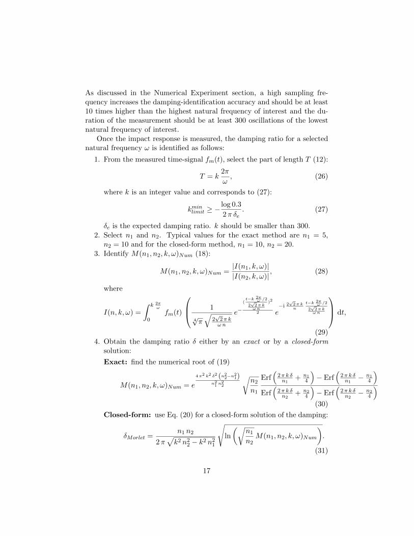
As discussed in the Numerical Experiment section, a high sampling fre-quency increases the damping-identification accuracy and should be at least10 times higher than the highest natural frequency of interest and the du-ration of the measurement should be at least 300 oscillations of the lowestnatural frequency of interest.

Once the impact response is measured, the damping ratio for a selectednatural frequency ω is identified as follows:

1. From the measured time-signal fm(t), select the part of length T (12):

T = k2π

ω, (26)

where k is an integer value and corresponds to (27):

kminlimit ≥ −log 0.3

2π δe. (27)

δe is the expected damping ratio. k should be smaller than 300.

2. Select n1 and n2. Typical values for the exact method are n1 = 5,n2 = 10 and for the closed-form method, n1 = 10, n2 = 20.

3. Identify M(n1, n2, k, ω)Num (18):

M(n1, n2, k, ω)Num =|I(n1, k, ω)||I(n2, k, ω)| , (28)

where

I(n, k, ω) =

∫ k 2πω

0fm(t)

1

4√π

√2√2π kω n

e−(t−k 2π

ω /2

2√2π kω n

)2

2 e−i 2

√2π kn

t−k 2πω /2

2√2π kω n

dt,

(29)

4. Obtain the damping ratio δ either by an exact or by a closed-formsolution:

Exact: find the numerical root of (19)

M(n1, n2, k, ω)Num = e

4π2 k2 δ2 (n22−n21)n21 n

22

√n2n1

Erf(2π k δn1

+ n14

)− Erf

(2π k δn1− n1

4

)Erf(2π k δn2

+ n24

)− Erf

(2π k δn2− n2

4

)(30)

Closed-form: use Eq. (20) for a closed-form solution of the damping:

δMorlet =n1 n2

2π√k2 n22 − k2 n21

√ln

(√n1n2

M(n1, n2, k, ω)Num

).

(31)

17

Figure 9 shows a noise-free damped signal that is 30 oscillations in length(k = 30).

0 5 10 15 20 25 30-1.0

-0.5

0.0

0.5

1.0

Oscilatons

Amplitude

Measured signal fm(t)

Re(ψu,s) at n2

Re(ψu,s) at n1

Figure 9: Typical measured (noise-free) signal and the real part of the Morlet wavelet atn1 = 5 and n2 = 10.

Compared to damping identification with the CWT based on logarith-mic decay, the damping identification using Eq.(20) is relatively easy touse and is not affected by the edge effect and requires significantly lesscomputational time. In [9, 10], where CWT damping identification wasresearched, the computationally demanding CWT was calculated with arelatively dense time-frequency grid; even with the cross-sections dampingidentification method [4] that requires only one frequency point the CWTneeds to be calculated with a relatively dense time grid. In [9, 10] the time-grid had more than 100 points. In this research the discussed Morlet-WaveMethod requires similar computational operations as the CWT; however,twice at only one time-frequency point. Neglecting other numerical opera-tions (the least-squares in the CWT and the root-finding in the Morlet-Wavemethod) the new method is approximately 50 or more times faster than theestablished CWT damping-identification methods. An exact analysis of thenumerical load depends on the damping-identification parameters of theCWT and the wave method and is beyond the scope of this research. Atthe same time, the advantages of the damping-identification techniques withthe CWT are preserved.

18

7. Conclusion

This study introduces a new viscous damping-identification method basedon the Morlet wavelet. The method is a combination of the continuouswavelet transform and the finite integral of the Morlet wavelet. With the ap-proximations given in the appendix, the Exact Morlet-wave (MW) damping-identification method is obtained, and by further simplifying a Closed-Form,Morlet-wave, damping-identification method is possible. While preservingthe CWT characteristics of the damping-identification of multi-degree-of-freedom systems, the accuracy of the identification and the resistance tonoise, the presented wave method is numerically significantly less demand-ing (approximately 50 times and more) and also completely overcomes theedge-effect problem of the CWT. For signals with a relatively high noiselevel, the root-finding Exact-MW identification method is needed; however,for signals with moderate noise the Closed-Form MW method gives an ac-curate solution.Compared to the CWT based damping-identification the MW based damping-identification hides the details of ridge/skeleton extraction and the regressionanalysis and therefore the MW based procedure is easily used as a “black-box” method; this can be considered an advantage, but also a disadvantageas the misuse of the method is harder to identify.In this research it was found that the Exact MW method damping-identificationis accurate to within 10% at medium damped (damping ratio: 10−1-10−2)signals with up to 5 dB noise; if the sampling rate is very high (50 to 100times faster than the frequency analyzed) a 10% accuracy is reached, evenfor a very high level of noise (up to -5 dB). For signals with small damping(damping ratio: 10−3-10−4) the 10% accuracy is reached at signals with lessthan 20 dB noise. Furthermore, for ultra-small damping (damping ratio:10−5-10−6) a 10% accuracy is only possible on a noise-free signal (120 dB).An investigation on closely spaced frequencies showed that the analysis isaccurate within 20% at a single frequency-spread of the MW damping-identification method, while at three frequency-spreads the accuracy is within5%.A comparison of the two presented methods, the Exact and the Closed-Form,showed that the Closed-Form method, while being simpler and giving closed-form solutions, is less resistant to noise (approximately 10 dB).

19

Appendix A. Finite Integral of Morlet Wave

In this section the complex integral given in Eq. (16):

I(n, k, ω) =

∫ T

0

(X e−δ ω t cos(ω t− ϕ)

) 1

4√π

√2√2π kω n

e−(t−k 2π

ω /2

2√2π kω n

)2

2 e−i 2

√2π kn

t−k 2πω /2

2√2π kω n

dt,(A.1)

is discussed with the focus on finding the absolute value |I(n, k, ω)|.Using symbolic integration techniques, Eq. (A.1) can be rewritten as:

I(n, k, ω) = −(π

2

)3/4X

√k

nωeπ k (4π k δ2−n2 (i+δ))

n2︸ ︷︷ ︸A

(BC +D), (A.2)

where:

B = e16π2 k2 (1+i δ)

n2−iϕ (A.3)

C = Erf

(2π k δ

n− n

4

)− Erf

(2π k δ

n+n

4

)(A.4)

D = eiϕ(

Erf

(−n

2 − 8π k (δ − 2 i)

4n

)− Erf

(n2 + 8π k (δ − 2 i)

4n

))(A.5)

For typical values of the time-spread parameter n, the number of os-cillations k and the damping ratio δ the Eq.(A.2) results in numericallymanageable numbers; however, the part B results in very high numbers thatare numerically impossible to deal with. Consequentially, the main goal ofthis section is to simplify and approximate the absolute value |I(n, k, ω| fortypical parameters: The absolute value |I(n, k, ω)| is (A.1):

|I(n, k, ω)| = |A (BC +D)| = |A| |BC +D| (A.6)

|I(n, k, ω)| can be approximated with:

|I(n, k, ω)| ≈ |A| |B| |C|, (A.7)

if the following assumption is true:

|D| � |B| |C|. (A.8)

20

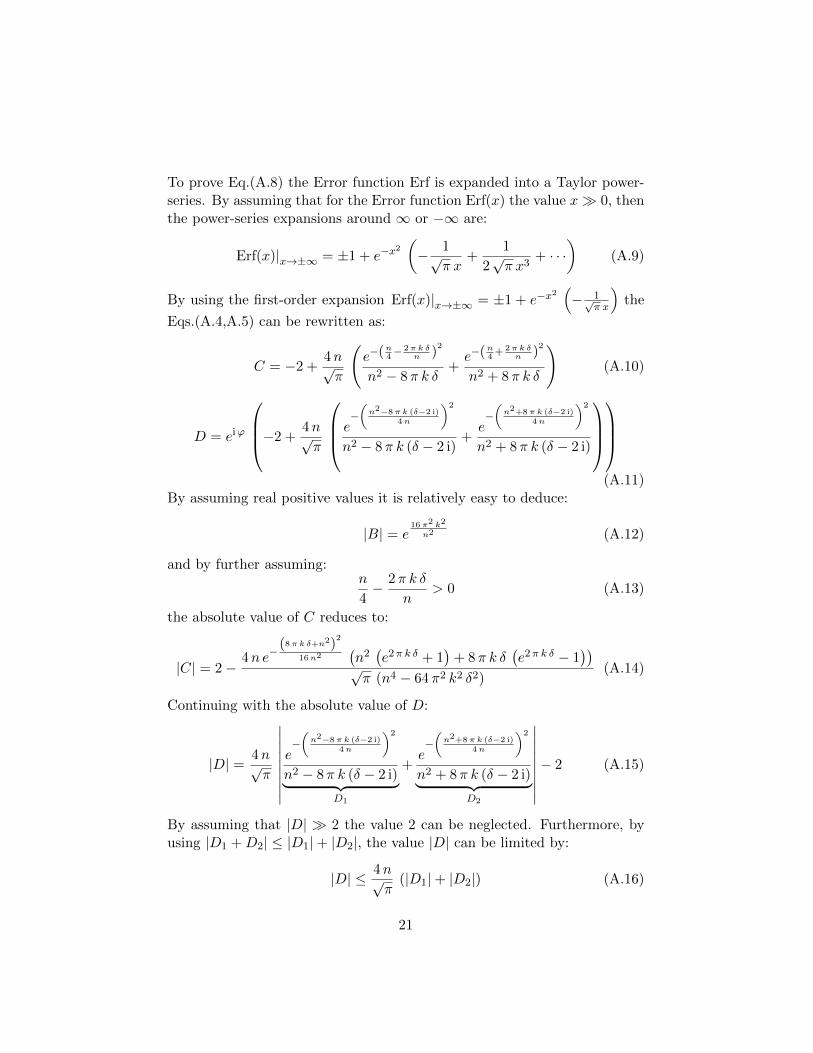
To prove Eq.(A.8) the Error function Erf is expanded into a Taylor power-series. By assuming that for the Error function Erf(x) the value x� 0, thenthe power-series expansions around ∞ or −∞ are:

Erf(x)|x→±∞ = ±1 + e−x2

(− 1√

π x+

1

2√π x3

+ · · ·)

(A.9)

By using the first-order expansion Erf(x)|x→±∞ = ±1 + e−x2(− 1√

π x

)the

Eqs.(A.4,A.5) can be rewritten as:

C = −2 +4n√π

(e−(n4−

2π k δn )

2

n2 − 8π k δ+e−(n4+

2π k δn )

2

n2 + 8π k δ

)(A.10)

D = eiϕ

−2 +4n√π

e−(n2−8π k (δ−2 i)

4n

)2

n2 − 8π k (δ − 2 i)+e−(n2+8π k (δ−2 i)

4n

)2

n2 + 8π k (δ − 2 i)

(A.11)

By assuming real positive values it is relatively easy to deduce:

|B| = e16π2 k2

n2 (A.12)

and by further assuming:n

4− 2π k δ

n> 0 (A.13)

the absolute value of C reduces to:

|C| = 2− 4n e−(8π k δ+n2)

2

16n2(n2(e2π k δ + 1

)+ 8π k δ

(e2π k δ − 1

))√π (n4 − 64π2 k2 δ2)

(A.14)

Continuing with the absolute value of D:

|D| = 4n√π

∣∣∣∣∣∣∣∣∣e−(n2−8π k (δ−2 i)

4n

)2

n2 − 8π k (δ − 2 i)︸ ︷︷ ︸D1

+e−(n2+8π k (δ−2 i)

4n

)2

n2 + 8π k (δ − 2 i)︸ ︷︷ ︸D2

∣∣∣∣∣∣∣∣∣− 2 (A.15)

By assuming that |D| � 2 the value 2 can be neglected. Furthermore, byusing |D1 +D2| ≤ |D1|+ |D2|, the value |D| can be limited by:

|D| ≤ 4n√π

(|D1|+ |D2|) (A.16)

21

0.001 0.01 0.11

10

100

1000

104

105

106

δ

|B||C

|/|D

∗ |

Figure A.10: |B| |C|/|D∗| vs. δ for typical parameter.

assuming real positive values, Eq.(A.16) can be deduced to:

|D| ≤4n

(1√

256π2 k2+(8π k δ+n2)2+ e2π k δ√

256π2 k2+(n2−8π k δ)2

)e−

(8π k (δ−2)+n2)(8π k (δ+2)+n2)16n2

√π

(A.17)Fig. A.10 shows the |B| |C|/|D∗| versus the damping factor for typical values:n = 10, k = 30 (|D∗| is the upper limit of |D| Eq.(A.17)); it is clear that theassumption of Eq.(A.8) is valid only if the assumption (A.13) is valid. FromEq. (A.13) it follows that for a selected time-spread parameter n and thenumber of oscillations k the theoretically identified damping ratio is limitedby (A.13):

δ ≤ n2

8π k. (A.18)

Finally, it follows from (A.7)

|I(n, k, ω)| ≈ X(π

4

)4/3 √ k

nωeπ k δ (4π k δ−n2)

n2

(Erf

(2π k δ

n+n

4

)− Erf

(2π k δ

n− n

4

)),

(A.19)where |C| was deduced from Eq. (A.4) and |A| in Eq. (A.7) assuming realpositive values was simplified to:

|A| = X(π

2

)3/4eπ k (4π k (δ2−4)−n2 δ)

n2

√k

nω(A.20)

22

References

[1] W. Staszewski, Identification of damping in mdof systems using time-scale decomposition, Journal of Sound and Vibration 203 (2) (1997)283–305.

[2] M. Prandina, J. E. Mottershead, E. Bonisoli, An assessment of dampingidentification methods, Journal of Sound and Vibration 323 (3-5) (2009)662–676. doi:10.1016/j.jsv.2009.01.022.

[3] F. Magalhaes, A. Cunha, E. Caetano, R. Brincker, Damping estima-tion using free decays and ambient vibration tests, Mechanical Systemsand Signal Processing In Press, Corrected Proof (2009) –. doi:DOI:10.1016/j.ymssp.2009.02.011.

[4] W. Staszewski, Identification of non-linear systems using multi-scaleridges and sceletons of the wavelet transform, Journal of Sound andVibration 214 (4) (1998) 639–658.

[5] M. Ruzzene, A. Fasana, L. Garibaldi, B. Piombo, Natural frequenciesand dampings identification using wavelet transform: Application toreal data, Mechanical Systems and Signal Processing 11 (2) (1997) 207–218.

[6] C. H. Lamarque, S. Pernot, A. Cuer, Damping identification in multi-degree-of-freedom systems via a wavelet-logarithmic decrement-part1:theory, Journal of Sound and Vibration 235 (3) (2000) 361–374.

[7] S. Hans, E. Ibraim, S. Pernot, C. Boutin, C. H. Lamarque, Damp-ing identification in multi-degree-of-freedom systems via a wavelet-logarithmic decrement-part 2:study of a civil engineering building, Jour-nal of Sound and Vibration 235 (3) (2000) 375–403.

[8] R. Ghanem, F. Romeo, A wavelet-based approach for the identifica-tion of linear time-varying dynamical systems, Journal of Sound andVibration 234 (4) (2000) 555–576.

[9] J. Slavic, I. Simonovski, M. Boltezar, Damping identification usinga continuous wavelet transform: Application to real data, Journal ofSound and Vibration 262 (2003) 291–307.

[10] M. Boltezar, J. Slavic, Enhancements to the continuous wavelet trans-form for damping identifications on short signals, Mechanical Systemsand Signal Processing 18 (5) (2004) 1065–1076.

23

[11] J. Lardies, S. Gouttebroze, Identification of modal parameters using thewavelet transform, International Journal of Mechanical Sciences 44 (11)(2002) 2263–2283. doi:10.1016/S0020-7403(02)00175-3.

[12] J. Lardies, M. Ta, M. Berthillier, Modal parameter estimation basedon the wavelet transform of output data, Archive of Applied Mechanics73 (9-10) (2004) 718–733. doi:10.1007/s00419-004-0329-6.

[13] T. Le, P. Argoul, Continuous wavelet transform for modal identificationusing free decay response, Journal of Sound and Vibration 277 (1-2)(2004) 73–100. doi:10.1016/j.jsv.2003.08.049.

[14] H. Yin, D. Duhamel, P. Argoul, Natural frequencies and dampingestimation using wavelet transform of a frequency response func-tion, Journal of Sound and Vibration 271 (3-5) (2004) 999–1014.doi:10.1016/j.jsv.2003.03.002.

[15] S. Erlicher, P. Argoul, Modal identification of linear non-proportionallydamped systems by wavelet transform, Mechanical Systems and SignalProcessing 21 (3) (2007) 1386–1421. doi:10.1016/j.ymssp.2006.03.010.

[16] M. Cesnik, J. Slavic, M. Boltezar, Spatial-Mode-Shape Identificationusing a Continuous Wavelet Transform, Strojniski vestnik-Journal ofMechanical Engineering 55 (5) (2009) 277–285.

[17] S.-L. Chen, J.-J. Liu, H.-C. Lai, Wavelet analysis for identification ofdamping ratios and natural frequencies, Journal of Sound and Vibration323 (1-2) (2009) 130 – 147. doi:DOI: 10.1016/j.jsv.2009.01.029.

[18] B. Yan, A. Miyamoto, A comparative study of modal parameter iden-tification based on wavelet and Hilbert-Huang transforms, Computer-Aided Civil and Infrastructure Engineering 21 (1) (2006) 9–23.

[19] Z. Li, M. Crocker, A study of joint time-frequency analysis-basedmodal analysis, IEEE Transactions on Instrumentation and Measure-ment 55 (6) (2006) 2335 – 2342. doi:DOI: 10.1109/TIM.2006.884137.

[20] J.-B. Tan, Y. Liu, L. Wang, W.-G. Yang, Identification of modal pa-rameters of a system with high damping and closely spaced modesby combining continuous wavelet transform with pattern search, Me-chanical Systems and Signal Processing 22 (5) (2008) 1055–1060.doi:10.1016/j.ymssp.2007.11.017.

24

[21] Z. Yan, A. Miyamoto, Z. Jiang, Frequency slice wavelet transform fortransient vibration response analysis, Mechanical Systems and SignalProcessing 23 (5) (2009) 1474–1489. doi:10.1016/j.ymssp.2009.01.008.

[22] Z. Yan, A. Miyamoto, Z. Jiang, X. Liu, An overall theoretical descrip-tion of frequency slice wavelet transform, Mechanical Systems and Sig-nal Processing 24 (2) (2010) 491–507. doi:10.1016/j.ymssp.2009.07.002.

[23] A. Grossmann, J. Morlet, Decomposition of hardy function into squareintegrable wavelets of constant shape, SIAM Journal of MathematicalAnalysis and Applications 15 (4) (1984) 723–736.

[24] S. Mallat, A Wavelet Tour of Signal Processing, 2nd Edition, AcademicPress, 1999.

[25] I. Simonovski, M. Boltezar, The norms and variances of the gabor,morlet and general harmonic wavelet functions, Journal of Sound andVibration 264 (3) (2003) 545–557.

[26] W. Thomson, Theory of Vibration with Applications, 4th Edition, Lon-don: Chapman and Hall, 1993.

[27] C. Beards, Structural Vibration: Analysis and Damping, Arnold, 1996.

[28] J. Tukey, Exploratory Data Analysis, Addison-Wesley, Reading, MA,1977.

25