Nov. 3, 2015 Leachman - Cycle Time 1 Cycle Time Management Prof. Rob Leachman University of California at Berkeley Nov. 3, 2015

Welcome message from author
This document is posted to help you gain knowledge. Please leave a comment to let me know what you think about it! Share it to your friends and learn new things together.
Transcript
Nov. 3, 2015 Leachman - Cycle Time 1
Cycle Time Management
Prof. Rob LeachmanUniversity of California
at Berkeley
Nov. 3, 2015
Nov. 3, 2015 Leachman - Cycle Time 2
Agenda• Definitions of cycle time
• Cycle time trends in the semiconductor
industry
• Reminder of Entitlement Cycle Time and
the Execution Gap
• General strategies and theory for
scheduling and production control
• Case-studies in cycle time reduction
Nov. 3, 2015 Leachman - Cycle Time 3
Definitions of related terms• Process flow – the series of manufacturing steps
traversed by manufacturing lots of a particular product type or particular product family– In semiconductor fabrication, typically, lots are started
containing 25 wafers of a single product
• WIP (work-in-process) – the manufacturing lots in the factory not yet completed
• Moves – the number of wafers passed through one or more manufacturing steps within a short time horizon such as a production shift– One move = one wafer completing one step
Nov. 3, 2015 Leachman - Cycle Time 4
Definitions of Cycle Time
• Cycle time from customer point of view (“lead time”) is the time from order placed until order received= design, paperwork, data entry and communication time
+ manufacturing time (if any)
+ interplant shipment time (if any)
+ safety time (if any)
+ customer shipment time
Nov. 3, 2015 Leachman - Cycle Time 5
Definitions of Cycle Time (cont.)
• Cycle time from manufacturing point of view(“cycle time”, “turn-around time” or “flow time”)
• Total manufacturing cycle time is the elapsed time from lot creation to lot completion
– includes process time, transport time, queue time, hold time across all steps of the process flow
• Cycle time for a process step is the average time from track-out of previous step to track-out of this step
Nov. 3, 2015 Leachman - Cycle Time 6
Definitions of Cycle Time (cont.)
• Standard cycle time is time to process one lot without interference (includes process time and move time but excludes queue time and hold time)
– standard cycle time for each process step
– standard cycle time for whole process flow
• Standard cycle time remains fixed until the process spec, equipment, or lot size is changed. (It is also called theoretical cycle time.)
Nov. 3, 2015 Leachman - Cycle Time 7
Measures of Cycle Time• “Static cycle time” is calculated from the elapsed
time for each lot. Usually, when one says “cycle time” one means “static cycle time”.
• “Dynamic cycle time” adds up the current average cycle time for each process step to estimate current cycle time from fab start to fab out.
• “Throughput time” (TPT) for a process step is calculated from the “WIP turns”. TPT for the factory is the sum of TPT’s for each process step:
TPT = 0.5 (EOH + BOH) / (Moves per period)(EOH = ending on-hand WIP, BOH = beginning on-hand)
Nov. 3, 2015 Leachman - Cycle Time 8
Measures of Cycle Time (cont.)
• Throughput time (TPT) implicitly assumes all lots are interchangeable.
• Dynamic cycle time is a good snapshot of current state of the fab, but is typically not
achievable by any particular lot.
• Typically (but not always),
Static cycle time > Dynamic cycle time > TPT
Nov. 3, 2015 Leachman - Cycle Time 9
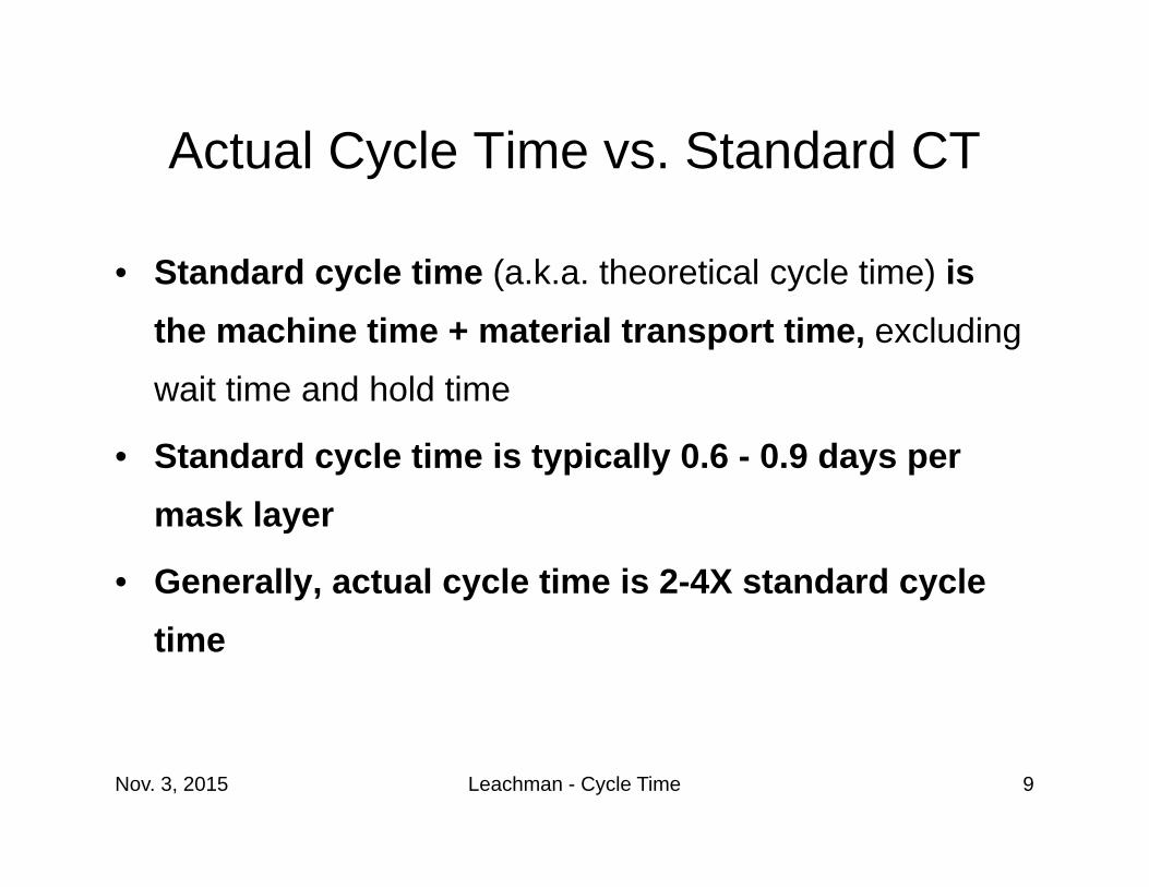
Actual Cycle Time vs. Standard CT
• Standard cycle time (a.k.a. theoretical cycle time) is the machine time + material transport time, excluding
wait time and hold time
• Standard cycle time is typically 0.6 - 0.9 days per mask layer
• Generally, actual cycle time is 2-4X standard cycle time
Nov. 3, 2015 Leachman - Cycle Time 10
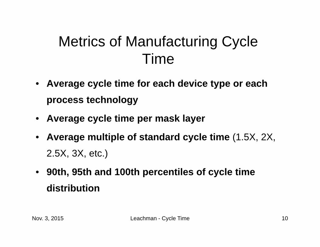
Metrics of Manufacturing Cycle Time
• Average cycle time for each device type or each process technology
• Average cycle time per mask layer
• Average multiple of standard cycle time (1.5X, 2X,
2.5X, 3X, etc.)
• 90th, 95th and 100th percentiles of cycle time distribution
Nov. 3, 2015 Leachman - Cycle Time 11
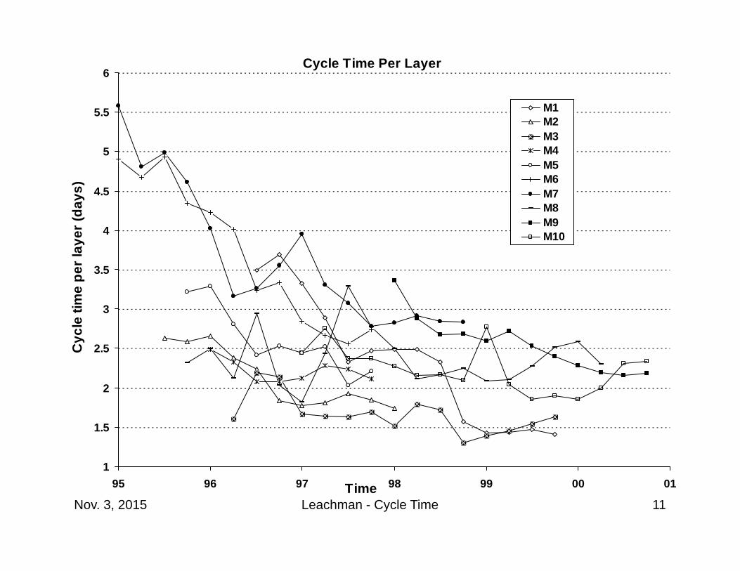
Cycle Time Per Layer
1
1.5
2
2.5
3
3.5
4
4.5
5
5.5
6
95 96 97 98 99 00 01Time
Cyc
le ti
me
per l
ayer
(day
s)
M1M2M3M4M5M6M7M8M9M10
Nov. 3, 2015 Leachman - Cycle Time 12
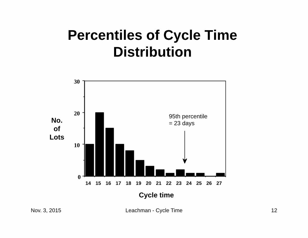
Percentiles of Cycle Time Distribution
14 15 16 17 18 19 20 21 22 23 24 25 26 270
10
20
30
95th percentile = 23 daysNo.
ofLots
Cycle time
Nov. 3, 2015 Leachman - Cycle Time 13
Industry trends• At most fabs, cycle time per mask layer trends
downwards over the fab life
– Cycle time is worse in the newest fabs of a company
– During transition to and ramp-up of new products,
cycle time often gets worse
• Traditionally, foundry fabs tended to focus on cycle time more than fabs making commodity products
– But some memory companies focus intensely on cycle
time, and some foundry companies do not
Nov. 3, 2015 Leachman - Cycle Time 14
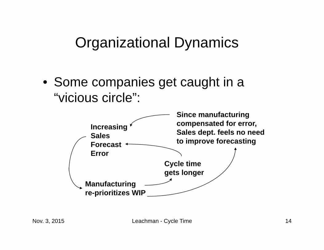
Organizational Dynamics
• Some companies get caught in a “vicious circle”:
IncreasingSalesForecastError
Manufacturingre-prioritizes WIP
Cycle time gets longer
Since manufacturingcompensated for error,Sales dept. feels no needto improve forecasting
Nov. 3, 2015 Leachman - Cycle Time 15
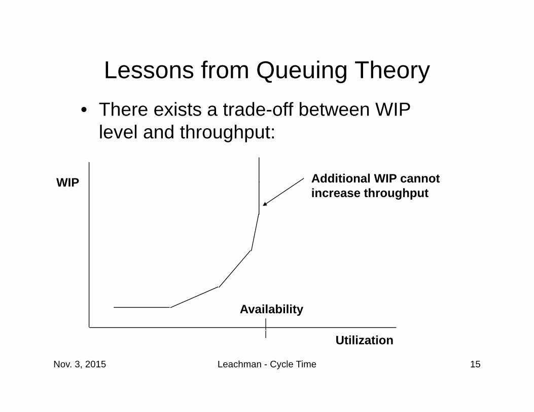
Lessons from Queuing Theory• There exists a trade-off between WIP
level and throughput:
Utilization
WIP
Availability
Additional WIP cannotincrease throughput
Nov. 3, 2015 Leachman - Cycle Time 16
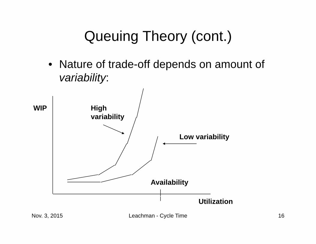
Queuing Theory (cont.)
• Nature of trade-off depends on amount of variability:
Utilization
WIP
Availability
Highvariability
Low variability
Nov. 3, 2015 Leachman - Cycle Time 17
Queuing Theory (cont.)
• Sources of variability:
– Fluctuating production workload, particularly if
capacity becomes overloaded or under-loaded
– Machine down time or operator absence
– Inflexible machine allocation
– Setups and test runs, large-batch production runs
– Changed product priorities, hot lots
– Lack of good scheduling and WIP management
Nov. 3, 2015 Leachman - Cycle Time 18
Little’s Conservation Law
• A process flow in steady-state obeys Little’s Law:
WIP = (production rate) * (cycle time)
• This law also applies to an individual process step or a series of steps
• Implication: cycle time reduction requires reduced WIP and/or higher throughput
Nov. 3, 2015 Leachman - Cycle Time 19
Components of cycle time and WIP
• Let’s expand Little’s Law:
WIP = (production rate) * (cycle time)
= (production rate) * (standard cycle time + wait time)
= {(production rate) * (standard cycle time)}
+ {(production rate) * (wait time)}
Total WIP = {Active WIP} + {Buffer WIP}
Nov. 3, 2015 Leachman - Cycle Time 20
WIP and Cycle Time (cont.)
• The Buffer WIP is the result of variability in the flow of the WIP
• Perfectly uniform WIP flow, consistent with bottleneck capacity -> no queues -> no buffer
• The more variability there is, the bigger the average buffer, and the longer the cycle time
Nov. 3, 2015 Leachman - Cycle Time 21
WIP and Cycle Time (cont.)
• If the WIP level in a process step or a group of steps
drops below the Active WIP level, then the production
rate drops below target
• The bottleneck resource needs to maintain its Active WIP level all the time
• If the input flow of WIP is variable, a buffer is needed at the bottleneck to maintain the target production rate
Nov. 3, 2015 Leachman - Cycle Time 22
Fab dynamics• Because the process and equipment are fragile,
disruptions in the flow of lots and dislocations of the WIP are a way of life in the fab.– “Availability” – the fraction of time an equipment or process
is able to perform the desired manufacturing process
– WIP “bubbles” form behind points of process or equipment trouble
• There is a continuous challenge to recover a “good” WIP profile and to achieve the goals for lot movement.
Nov. 3, 2015 Leachman - Cycle Time 23
Theory of Constraints (TOC)• Factory production rate is production rate of bottleneck
work center
• The buffer WIP should be concentrated at the bottleneck
• Bottleneck implies certain amount of idle time at other
work stations
• Important to regulate bottleneck workload; other work centers should serve the bottleneck, not optimize themselves
Nov. 3, 2015 Leachman - Cycle Time 24
Bottleneck Machines
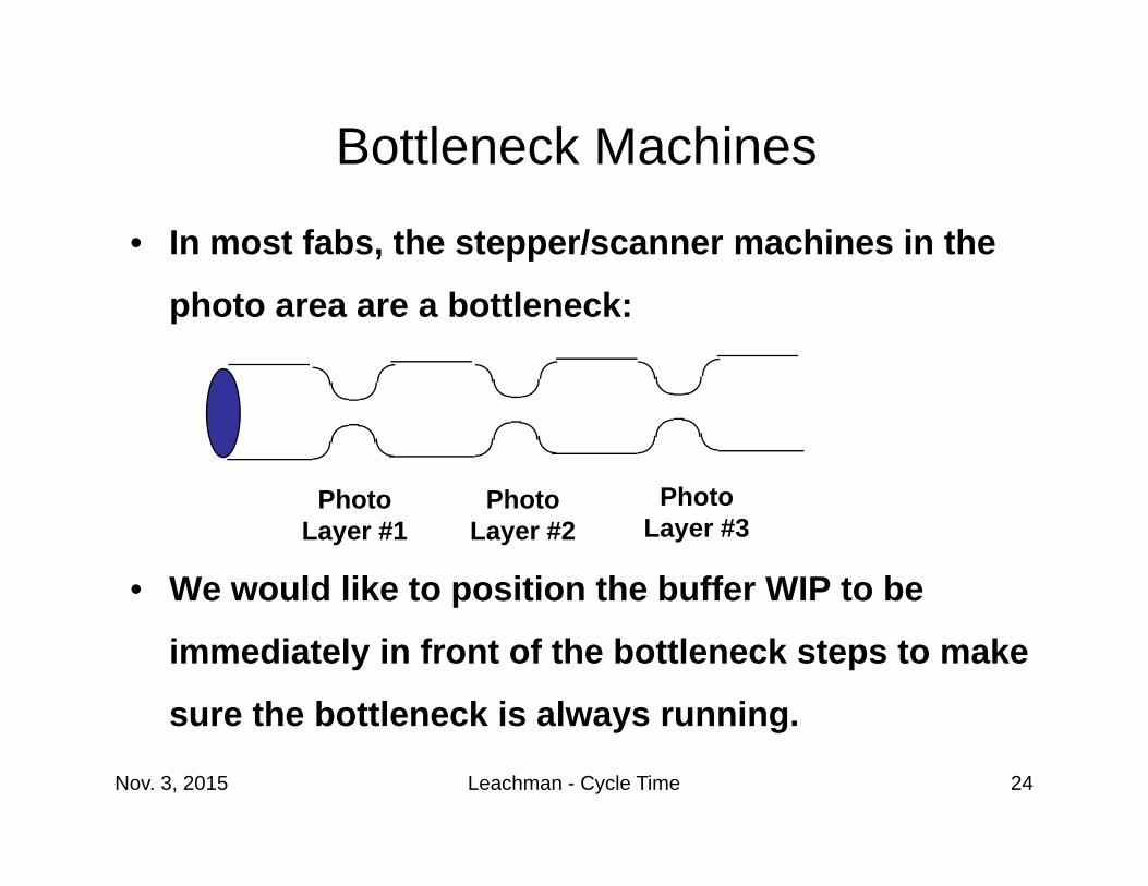
• In most fabs, the stepper/scanner machines in the
photo area are a bottleneck:
• We would like to position the buffer WIP to be
immediately in front of the bottleneck steps to make
sure the bottleneck is always running.
PhotoLayer #1
PhotoLayer #2
PhotoLayer #3
Nov. 3, 2015 Leachman - Cycle Time 25
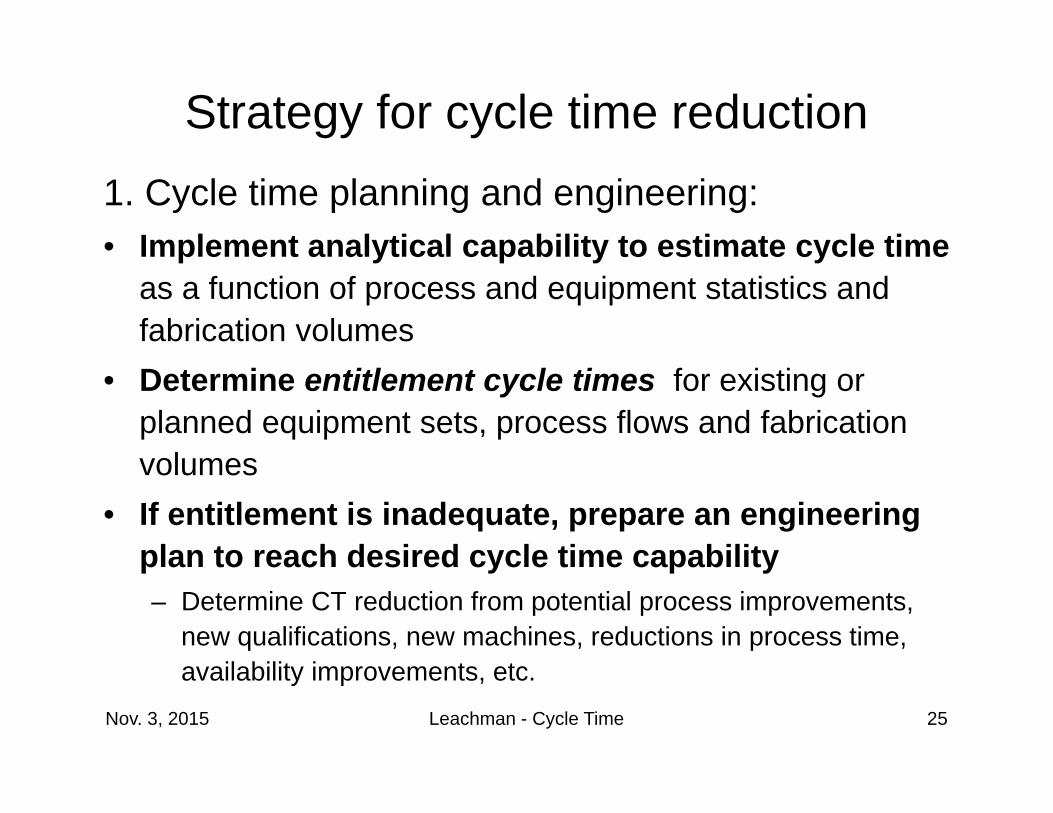
Strategy for cycle time reduction1. Cycle time planning and engineering:• Implement analytical capability to estimate cycle time
as a function of process and equipment statistics and fabrication volumes
• Determine entitlement cycle times for existing or planned equipment sets, process flows and fabrication volumes
• If entitlement is inadequate, prepare an engineering plan to reach desired cycle time capability– Determine CT reduction from potential process improvements,
new qualifications, new machines, reductions in process time, availability improvements, etc.
Nov. 3, 2015 Leachman - Cycle Time 26
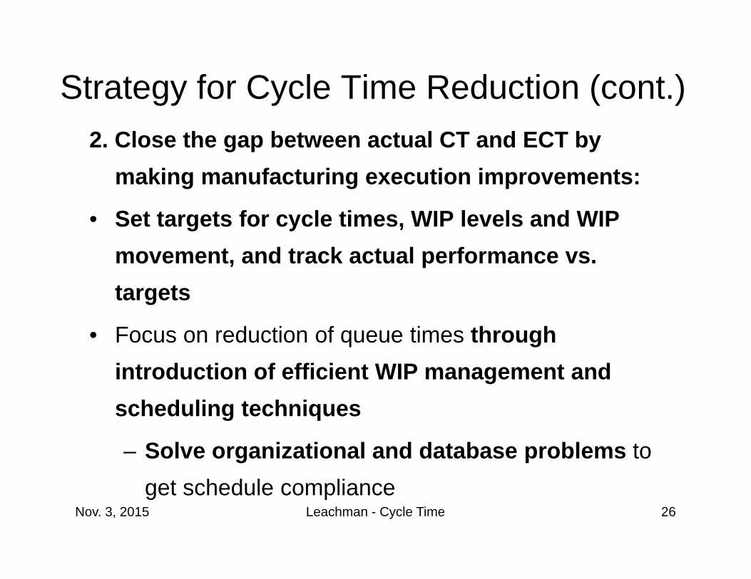
Strategy for Cycle Time Reduction (cont.)2. Close the gap between actual CT and ECT by
making manufacturing execution improvements:
• Set targets for cycle times, WIP levels and WIP movement, and track actual performance vs. targets
• Focus on reduction of queue times through introduction of efficient WIP management and scheduling techniques
– Solve organizational and database problems to get schedule compliance
Nov. 3, 2015 Leachman - Cycle Time 27
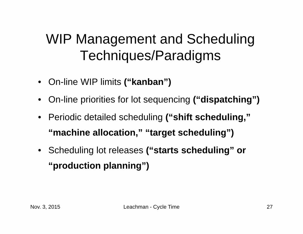
WIP Management and SchedulingTechniques/Paradigms
• On-line WIP limits (“kanban”)
• On-line priorities for lot sequencing (“dispatching”)
• Periodic detailed scheduling (“shift scheduling,” “machine allocation,” “target scheduling”)
• Scheduling lot releases (“starts scheduling” or “production planning”)
Nov. 3, 2015 Leachman - Cycle Time 28
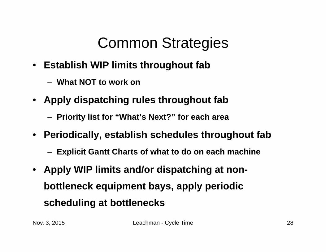
Common Strategies• Establish WIP limits throughout fab
– What NOT to work on
• Apply dispatching rules throughout fab– Priority list for “What’s Next?” for each area
• Periodically, establish schedules throughout fab– Explicit Gantt Charts of what to do on each machine
• Apply WIP limits and/or dispatching at non-bottleneck equipment bays, apply periodic scheduling at bottlenecks
Nov. 3, 2015 Leachman - Cycle Time 29
On-Line WIP Limits• “Just-in-time” WIP controls:• Pioneered in automobile industry where labor is
primary resource (a relatively flexible resource)
• When downstream WIP is too high, prevent machine or worker allocation to the process step
• Stop further WIP accumulation, force re-balancing of production line
• Gradual decrease in WIP limits is used to force manufacturing to make changes that reduce variability and permit linear flow.
Nov. 3, 2015 Leachman - Cycle Time 30
On-Line WIP Limits (cont.)
• “Just-in-time” methodology (cont.):
• An upper bound can be placed on WIP at each operation (or group of operations); if WIP limit is reached, upstream operation must stop processing lots that go next to operation at WIP limit. This discipline prevents WIP from exceeding the upper bound.
• Underlying principle of “kanban” systems.
Nov. 3, 2015 Leachman - Cycle Time 31
Dispatching
• Dispatching - suggest which lot or recipe to process next when the machine finishes a lot or recipe
• Least slack dispatching rule:
– slack = (time until due date) – (remaining cycle time
to fab out )
• This rule maintains and restores orderly flow of lots
– reduces variability of lot flow
– suitable for low-volume order-based production
Nov. 3, 2015 Leachman - Cycle Time 32
Dispatching (cont.)Other common rules:• Critical Ratio = (time until due date) / (remaining
cycle time to fab out)– similar to least slack rule, except gives much more
attention to lots closer to the end of the process flow
• Setup compatibility (try not to break setup)• Batch compatibility (try to build up batch)• Starvation Index (prioritize lots heading to
bottleneck resource when bottleneck is underloaded)

Nov. 3, 2015 Leachman - Cycle Time 33
Agent-Based Scheduling• Create internal market mechanism whereby jobs
(lots and maintenance jobs) “bid” for equipment time
• When lot arrives in an equipment area, it solicits “bids” from machines and selects the best bid– “Appointment” calendars are updated accordingly
– Might bump other appointments
• Similar to traditional dispatching except lots choose machines instead of machines choose lots
Nov. 3, 2015 Leachman - Cycle Time 34
Machine Allocation, Shift Scheduling, Periodic Scheduling
• Basic ideas: assign machines to device-steps or recipes once per shift or once per half-shift or even more often. Set production targets.
• Allocate machines so as to re-balance WIP in line and to accelerate volume of products behind schedule. Maximize utilization of bottlenecks.
• Issues: How to measure balance of WIP? How to tell if
products are behind schedule? How to resolve
conflicting needs?
Nov. 3, 2015 Leachman - Cycle Time 35
Volume-Based Priorities• Ideal production quantity (IPQ):
– IPQ = (total output due up until target-cycle-time-
to-fab-out + one shift) - (actual fab outs to date) -
(actual downstream WIP)
• Least schedule score dispatching rule:
– Schedule score = - IPQ / (target output rate)
– Recipe with least score is dispatched first
• Similar to least slack rule, but works better in the case of volume production
Target Cycle Times• Underlying all dispatching methodologies is
some means of setting target cycle times for each step of each process flow– So we can determine if production output at a step is
on schedule or late• Issue: What should be the target cycle time?
Some methods used:– Scale actual cycle times or simulated cycle times to
add up to the start-to-end target– Apply a common multiplier of SCT to all steps– Deliberately establish buffers considering variability in
lot flow and bottlenecksNov. 3, 2015 Leachman - Cycle Time 36
Nov. 3, 2015 Leachman - Cycle Time 37
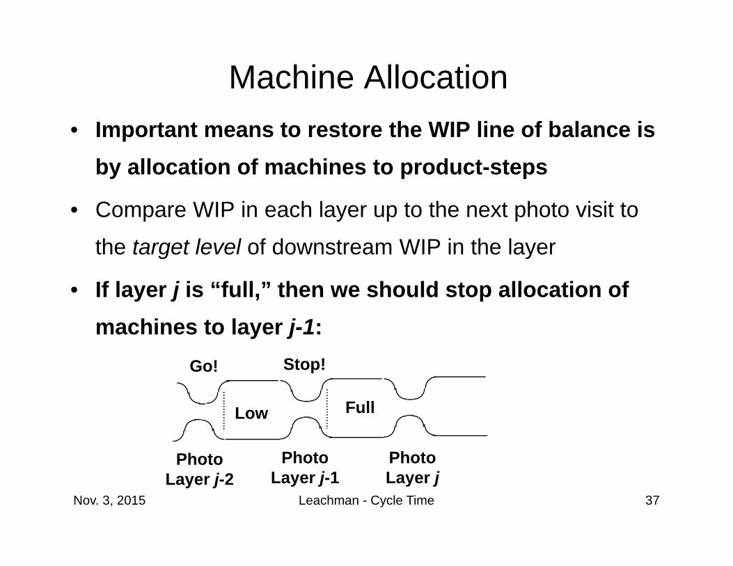
Machine Allocation• Important means to restore the WIP line of balance is
by allocation of machines to product-steps
• Compare WIP in each layer up to the next photo visit to
the target level of downstream WIP in the layer
• If layer j is “full,” then we should stop allocation of machines to layer j-1:
PhotoLayer j-1
PhotoLayer j
Full
Stop!
Low
Go!
PhotoLayer j-2
Nov. 3, 2015 Leachman - Cycle Time 38
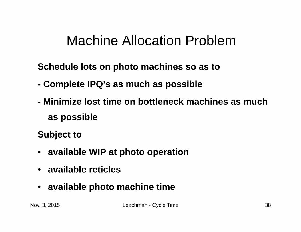
Machine Allocation Problem
Schedule lots on photo machines so as to
- Complete IPQ’s as much as possible
- Minimize lost time on bottleneck machines as much as possible
Subject to
• available WIP at photo operation
• available reticles
• available photo machine time
Nov. 3, 2015 Leachman - Cycle Time 39
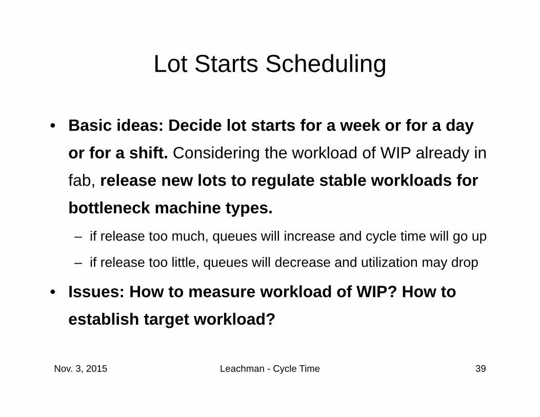
Lot Starts Scheduling
• Basic ideas: Decide lot starts for a week or for a day or for a shift. Considering the workload of WIP already in
fab, release new lots to regulate stable workloads for bottleneck machine types.– if release too much, queues will increase and cycle time will go up
– if release too little, queues will decrease and utilization may drop
• Issues: How to measure workload of WIP? How to establish target workload?
Nov. 3, 2015 Leachman - Cycle Time 40
Case Studies inImproving Manufacturing
Execution forCycle Time Reduction
Nov. 3, 2015 Leachman - Cycle Time 41
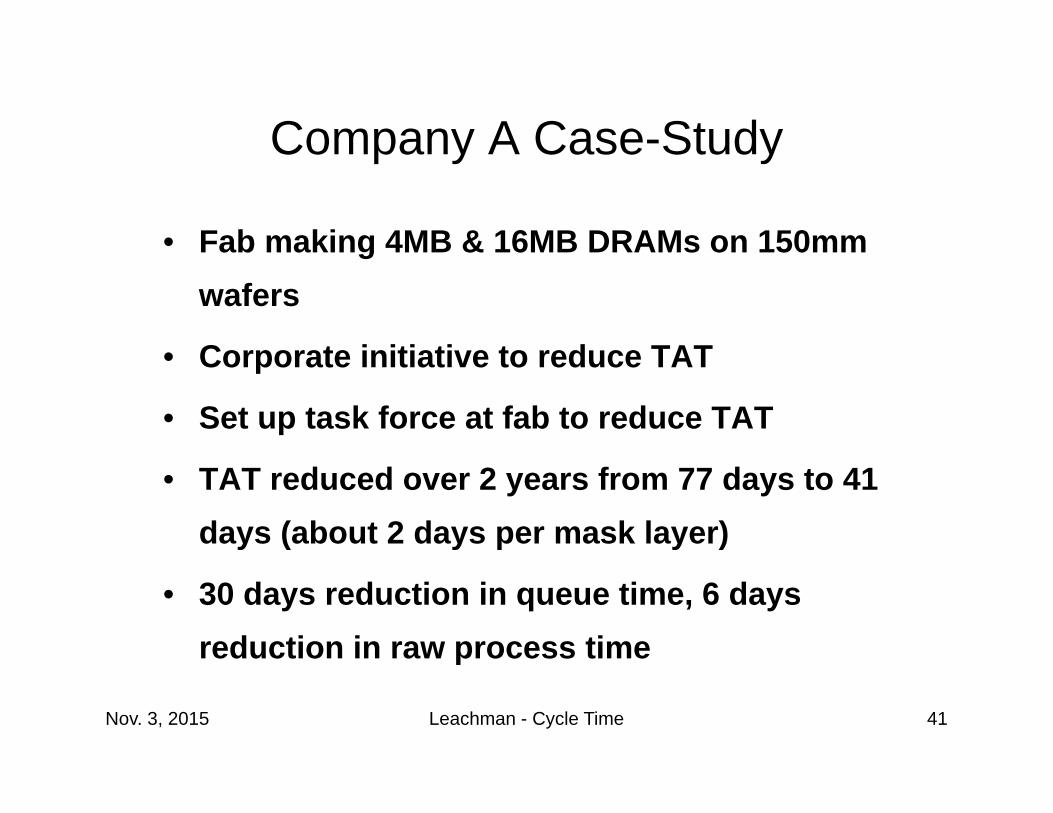
Company A Case-Study
• Fab making 4MB & 16MB DRAMs on 150mm wafers
• Corporate initiative to reduce TAT
• Set up task force at fab to reduce TAT
• TAT reduced over 2 years from 77 days to 41 days (about 2 days per mask layer)
• 30 days reduction in queue time, 6 days reduction in raw process time
Nov. 3, 2015 Leachman - Cycle Time 42
Company A Tactics
• Establish TAT goals by process step
• Monitor TAT goal vs. actual TAT and monitor production rate variation at each process step
• Each month, focus on four worst performers and try to fix in one month
Nov. 3, 2015 Leachman - Cycle Time 43
Company A Tactics (cont.)
• Found biggest issue was that small-volume lots or isolated lots waited huge amounts of time
– leaders and operators wanted to avoid doing
setups for them
• Changed scheduling policy to force setup of all operations frequently. They reduced some setup times (e.g., convert to external setup).
Nov. 3, 2015 Leachman - Cycle Time 44
Company A Tactics (cont.)• Focus on photo area. “If we control photo, we control the
fab.”
• They reduced photo WIP from 700 lots to 388 lots while maintaining throughput of 600 lots per day– Found that move-ins and move-outs were too disparate and
they were not meeting goals
– Queue would grow very fast any time there was a breakdown
– Simplified & expedited reticle changes, reduced need for test wafers, coordinated maintenance with WIP level
– Now, ins and outs are closer but still disparate; goals are now met.
Nov. 3, 2015 Leachman - Cycle Time 45
Company B Case-Study• Fab makes logic products on 125mm wafers
– Four process flows (many devices in each flow) using G Line steppers
• Corporate goal to reduce cycle time 25% per year
• Regular production management plus staff did project in fab to reduce cycle time
• In 6 months, cycle time was reduced from 2.1 days to 1.4 days per mask layer (theoretical cycle time was reduced by 30%, while fab cycle time was reduced to 1.5 times theoretical)
Nov. 3, 2015 Leachman - Cycle Time 46
Company B Tactics
• Analyze production rate and cycle time data by step
– Track variation of hourly output vs. target output rate
– Track actual TAT vs. target
• Kanban system implemented using video monitors
– Guides both production and maintenance activity
• Standardize processes to eliminate recipe changeovers
Nov. 3, 2015 Leachman - Cycle Time 47
Company B Tactics (cont.)
• Operators cross-trained to know all operations in
their equipment bay
• Photo coat-expose-develop steps all linked by robot into single operation (“photocluster”)
– Flexible configuration
• Fab layout re-arranged into “cells”; each cell
might have several photo machines, an inspect
area, several etch machines, 2 implanters, etc.
Nov. 3, 2015 Leachman - Cycle Time 48
Company B Tactics (cont.)
Fully automated company-wide production plan generated every weekend:
• Comprehends fab equipment capacity and reticle
supply
• Fab starts are capacity-feasible and reticle-feasible
• Changes in mix of process flow volumes are
restricted to be gradually phased in
• Fab WIP is never re-scheduled
Nov. 3, 2015 Leachman - Cycle Time 49
Company B Kanban System• Establish WIP limit for each process block (i.e., for
WIP tracking log points) in each process flow– WIP limit equals “active WIP” plus a ”buffer”. Estimate of active
WIP is based on production schedule and theoretical cycle time.
Buffer allows for WIP build-up during MTTR, MTTPM, etc. that
can be drawn back down in target amount of time when
equipment is up. Machine UPH and availability data are used.
– Limit calculated in wafers is rounded up for lot size– Computation of WIP limit implemented on computer
• Large video monitors hung from ceiling throughout fab to display Kanban controls
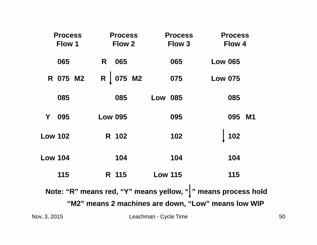
Nov. 3, 2015 Leachman - Cycle Time 50
ProcessFlow 1
ProcessFlow 2
ProcessFlow 3
ProcessFlow 4
065
075
085
095
102
104
115
065
075
085
095
102
104
115
065
075
085
095
102
104
115
065
075
085
095
102
104
115
Low
Low
Low
Low
Low
Low
Low
Y
R R
R
R
M2 M2
Note: “R” means red, “Y” means yellow, “ ” means process hold“M2” means 2 machines are down, “Low” means low WIP
M1
R
Nov. 3, 2015 Leachman - Cycle Time 51
Company B Kanban (cont.)
• Each monitor shows a matrix with columns for each process flow and rows for each process block
• Color scheme for matrix entries:
– Red means kanban stop; do not send any lots to
this block
– Yellow means caution; one more lot will reach
kanban limit
– Green means WIP level is OK; send more lots to
this block
Nov. 3, 2015 Leachman - Cycle Time 52
Company B Kanban (cont.)• Flashing entries in matrix display:
– This process flow is behind today’s schedule at this process block
• Symbols on matrix entries:
– “M2” means two machines in this process block are now down
– A down arrow means this process block is now on hold
– “Low” means WIP level in this block is low
Nov. 3, 2015 Leachman - Cycle Time 53
Company B Kanban (cont.)
• Operators and supervisors use display to decide what lots to process next (and to see who needs
help)
• Technicians and engineers use display to decide what trouble to work on first
• Managers can see trouble on the line as soon as it happens
• No hot lots are allowed.
Nov. 3, 2015 Leachman - Cycle Time 54
Comments on Company B• Video system and Kanban controls were
iteratively designed by production team with information team support.
• They estimate 15-20% of cycle time reduction came from photoclusters; 80-85% came from WIP reduction and changes forced by WIP reduction.
• At same time TAT was reduced to 1.2 days per mask layer, stepper throughput was increased from 550 to 750 aligns per stepper per day.
Nov. 3, 2015 Leachman - Cycle Time 55
Company C Case-Study
• Gate array ASIC producer
– 600 die types in four device families produced
at same time
– 1.2um down to 0.6um designs on G Line and I
Line steppers
• Most common lot size after option bank is 1 wafer; median lot size is 8 wafers
Nov. 3, 2015 Leachman - Cycle Time 56
Company C Case-Study (cont.)
• Reduced cycle time to 2 days per mask layer while maintaining output rate.
• Reduced variance of cycle time dramatically; difference between mean cycle time and 100th percentile of cycle time was reduced to about 2 days!
• Company routinely achieves 95% LIPAS on customer deliveries.
Nov. 3, 2015 Leachman - Cycle Time 57
Company C Tactics
• Customer lead time is based on 95th percentile of fab cycle time
• Fab line management evaluated by executives on basis of 100th percentile of cycle time,
• Cycle time goals by step were established. UPH goals for bottleneck equipment were established.
• Fab line management tracks actual cycle time and UPH very closely; managers meet with line supervisors three times per day.
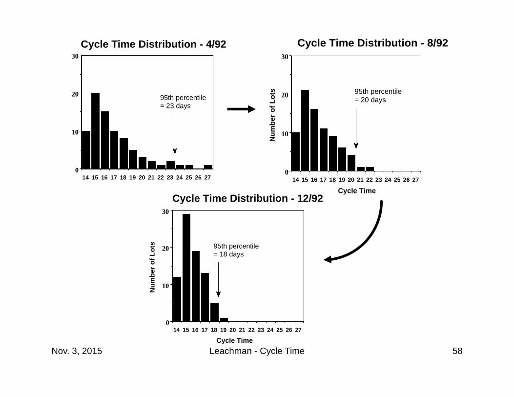
Nov. 3, 2015 Leachman - Cycle Time 58
14 15 16 17 18 19 20 21 22 23 24 25 26 270
10
20
30
Cycle Time Distribution - 8/92
Cycle Time
Num
ber o
f Lot
s 95th percentile = 20 days
14 15 16 17 18 19 20 21 22 23 24 25 26 270
10
20
30
Cycle Time
Num
ber o
f Lot
s
Cycle Time Distribution - 12/92
95th percentile= 18 days
14 15 16 17 18 19 20 21 22 23 24 25 26 270
10
20
30
95th percentile = 23 days
Cycle Time Distribution - 4/92
Nov. 3, 2015 Leachman - Cycle Time 59
Company C Tactics (cont.)
• Computerized lot dispatch: to select next lot for processing, operators follow priority list on computer screen. (Many setups are made.)
• Lots are prioritized based on least slack rule(slack equals lot due date minus remaining TAT to
get out of fab)
• Lot sequence negatively correlated with elapsed cycle time -> lower variance of lot cycle time
Nov. 3, 2015 Leachman - Cycle Time 60
Company C Tactics (cont.)
Out of 450 total lots, 15 lots are “prototype” lots, 20-30 “express” hot lots, and 15 “semi-express” lots
– express lots include re-starts resulting from lot scraps, critical customer needs, and lots very far behind schedule.
– “semi-express” lots are allocated “marketing expedites”.
– express and semi-express are prioritized ahead of regular lots.

Nov. 3, 2015 Leachman - Cycle Time 61
Company C Tactics (cont.)
• Real-time production planning of orders based on available fab capacity
– commit date given by Order Management
dept. only after finding slot in fab start queue.
No exceptions.
– fab line informed on-line about starts queue
Nov. 3, 2015 Leachman - Cycle Time 62
Company C Tactics (cont.)
• New focus: reduction of non-manufacturing time from customer lead time
• Tactics: develop and install new system encompassing automated order “configuration” (i.e., paperwork) and automated order scheduling through all factories
– integrate subcontract back end plants
– reduce safety time and administrative time
Nov. 3, 2015 Leachman - Cycle Time 63
Company D Case-Study
• 1990: Production planning was weak– planning cycle was once a month
– poor quality forecast
– much second-guessing by production teams
– planning cycle involved many participants and
negotiations
– high inventories, high WIP
– poor visibility to production plan, poor coordination of
factories, hard to determine delivery dates
Nov. 3, 2015 Leachman - Cycle Time 64
Company D Case-Study (cont.)
• 1990: On time delivery performance was poor
– sales went down fast, causing financial crisis
• Automated, optimization-based planning system was implemented (took 2 years; major data and organizational changes)
• Production plan regenerated every weekend
– fully automated, no negotiations
– urgent orders scheduled every day during the week
Nov. 3, 2015 Leachman - Cycle Time 65
Company D Results (cont.)
• WIP became “much higher quality,” i.e., much more aligned with market demand
• On time delivery improved from 75% to 95%
• Lead times and TATs went down sharply
• Sales went back up and company survived and even thrived
Nov. 3, 2015 Leachman - Cycle Time 66
Company D Tactics
• Demand forecasting system installed;marketing dept. continuously maintains database
of demands and priorities
• Capacity data bases and Product Code data bases installed; production dept. continuously
maintain databases of capacity and product
structure data
• Completely integrated scheduling of all factories according to data in databases
Nov. 3, 2015 Leachman - Cycle Time 67
Company D Tactics (cont.)
• Enforce manufacturing discipline by observing rules involving “corporate inventory points”:– no re-scheduling of WIP until next corporate inventory point
– no starts scheduled out of corporate inventory point unless
(1) required for market demand, and (2) capacity available
(after WIP flush) to reach next corporate inventory point
within normal TAT.
– “market demand” includes only orders (BTO product) or
also includes forecast (BTF product), as decided by
marketing dept.
Nov. 3, 2015 Leachman - Cycle Time 68
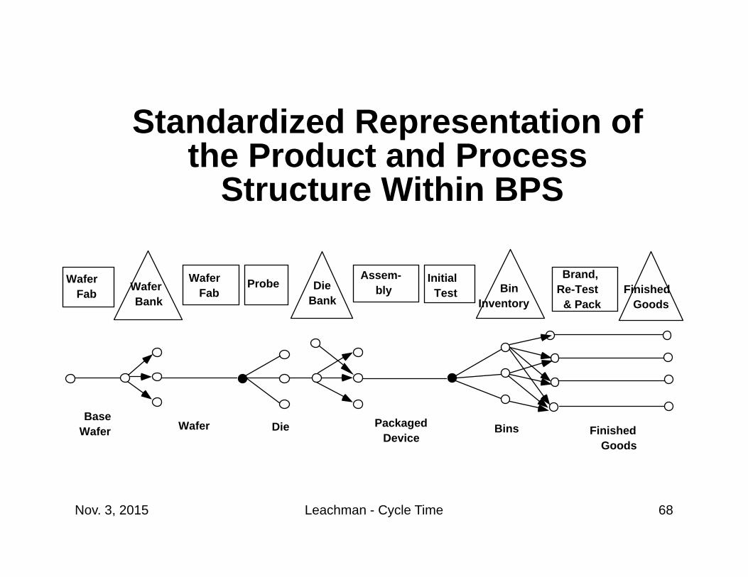
Die Bank
Bin Inventory
Assem- bly
Initial Test
Brand, Re-Test
& Pack
Packaged Device Finished
Goods
Wafer Fab
Probe
DieWaferBase
Wafer
Finished Goods
Standardized Representation of the Product and Process
Structure Within BPS
Bins
Wafer Bank
Wafer Fab
Nov. 3, 2015 Leachman - Cycle Time 69
Company D Tactics (cont.)
Implementation revealed organizational problems:
• Data quality was very poor and data ownership did not exist
• Factories did not want to flush out “dead WIP”
• Non-bottleneck plants did not want to slow down
• Non-bottleneck work centers did not want to do small lots and many setups
Necessary to enforce TOC philosophy
Nov. 3, 2015 Leachman - Cycle Time 70
Evaluation of Case-Studies
• Company A: focused on bottleneck and reduced variability (by reducing setup times and
run sizes and forcing linearity)
• Company B: used kanban to control WIP and reduced variability (by using on-line dispatching,
reducing setup times and run sizes, no re-
scheduling of WIP), and regulated workload on bottlenecks in weekly starts plan
Nov. 3, 2015 Leachman - Cycle Time 71
Evaluation of Case-Studies (cont.)
• Company C: reduced variability (used least
slack dispatching, no re-scheduling of WIP), and
regulated workload in starts plan
• Company D: reduced variability (no re-
scheduling of WIP), regulated workload on bottlenecks in weekly starts plan
Nov. 3, 2015 Leachman - Cycle Time 72
Lessons Learned• Cycle time reduction efforts must be made by
production team, with information team support
• Cycle time reduction efforts typically require improvements in information systems– Report accurate data on cycle time and variability
– Fab starts plan must keep up with changes in demand and
must regulate workload on bottleneck
– Control of lot dispatching needed to reduce variability
• Variability must be driven out of process
Related Documents