1 Industrial Engineering Design of Production Planning Systems for the Semiconductor Industry Prof. Robert C. Leachman Dept. of Industrial Engineering and Operations Research University of California at Berkeley March 2, 2013 Production Planning refers to the business processes for establishing target schedules for the outputs of factories, for scheduling the launch of new manufacturing lots in factories, for determining schedules for procurement of raw materials supporting new production, for scheduling the allocation and shipment of intermediate products for follow-on uses, and for quoting delivery dates in response to customer inquiries. Production planning is concerned with ensuring on-time delivery of customer orders, with ensuring the raw materials needed to support production are made available when required, and with determining the best deployment of supply-chain and manufacturing assets considering the available market opportunities. “Best” in this sense embraces both maximum expected cash flow to the company as well as wise management of the risks for excess inventory and lost sales. The business process for deciding changes to the asset base itself, i.e., purchase of new equipment, salvaging existing equipment, and increasing or decreasing staffing levels, is termed Capacity Planning, a related but different business process. Normally, the frequency of decision- making about changing the asset base is much less than the frequency of decision-making about how to deploy the assets. As we define it here, Capacity Planning precedes Production Planning, whereby Production Planning takes as given the asset base determined by the decisions made in Capacity Planning. Typically, the decisions of Production Planning are not expressed at a level of detail fully enabling manufacturing and supply-chain execution. Instead, Production Planning provides goals or targets and constraints for execution. A follow-on business process is required to enable execution in manufacturing, termed Factory Floor Scheduling. Factory Floor Scheduling takes as given the decisions made in Production Planning concerning factory input schedules and target output schedules, the availability of raw materials, and the allocation and shipping of intermediate products. Similarly, follow-on business processes may be required to fully enable shipments of intermediate products between supply-chain facilities, e.g., scheduling warehouse tasks or dispatching individual transportation shipments. Figure 1 displays the databases and business processes embraced by Production Planning in a company that manufactures its products. Starting in the upper right corner, customers engage with an Order Entry and Delivery Quotation System. This system keeps track of supply commitments to customers expressed as outstanding customer orders or as inventory commitments. The outstanding customer orders plus internally generated orders for replenishing contracted or targeted inventory levels are referred to as the Order Board. For a given product that is sold, the portion of finished goods inventory and planned output of finished goods not committed to any customer is termed the Product Availability or the Available-to-Promise quantity. Customers submit requests for delivery quotes to this system. Delivery quotes are calculated based on product availability. A time limit is attached to each quote; if the customer

Welcome message from author
This document is posted to help you gain knowledge. Please leave a comment to let me know what you think about it! Share it to your friends and learn new things together.
Transcript

1
Industrial Engineering Design of Production Planning Systems for the Semiconductor Industry
Prof. Robert C. Leachman Dept. of Industrial Engineering and Operations Research
University of California at Berkeley March 2, 2013
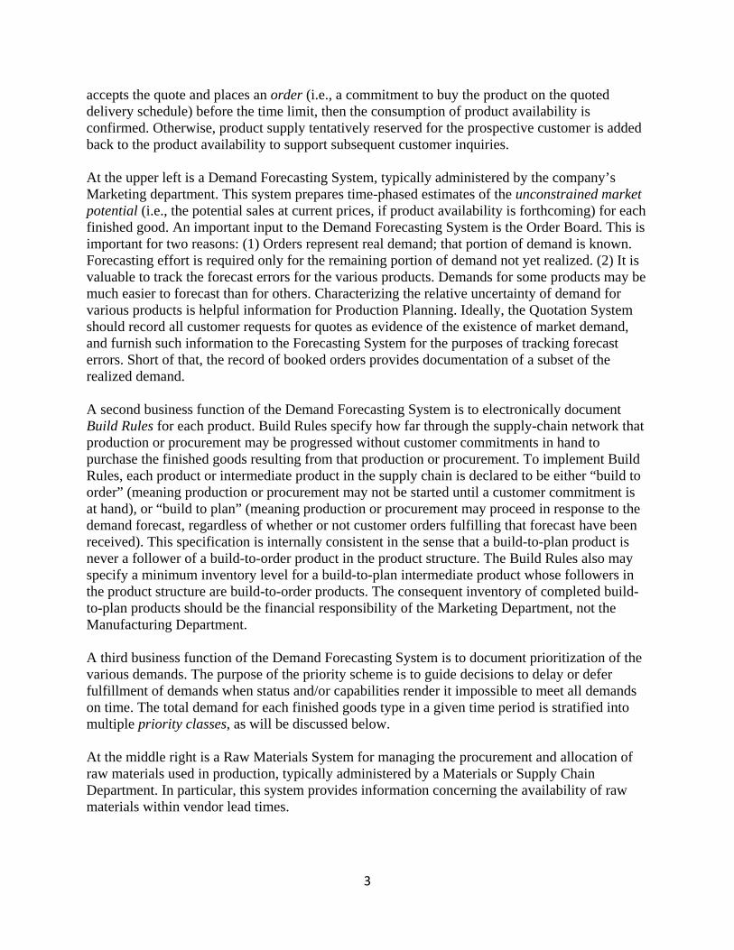
Production Planning refers to the business processes for establishing target schedules for the outputs of factories, for scheduling the launch of new manufacturing lots in factories, for determining schedules for procurement of raw materials supporting new production, for scheduling the allocation and shipment of intermediate products for follow-on uses, and for quoting delivery dates in response to customer inquiries. Production planning is concerned with ensuring on-time delivery of customer orders, with ensuring the raw materials needed to support production are made available when required, and with determining the best deployment of supply-chain and manufacturing assets considering the available market opportunities. “Best” in this sense embraces both maximum expected cash flow to the company as well as wise management of the risks for excess inventory and lost sales. The business process for deciding changes to the asset base itself, i.e., purchase of new equipment, salvaging existing equipment, and increasing or decreasing staffing levels, is termed Capacity Planning, a related but different business process. Normally, the frequency of decision-making about changing the asset base is much less than the frequency of decision-making about how to deploy the assets. As we define it here, Capacity Planning precedes Production Planning, whereby Production Planning takes as given the asset base determined by the decisions made in Capacity Planning. Typically, the decisions of Production Planning are not expressed at a level of detail fully enabling manufacturing and supply-chain execution. Instead, Production Planning provides goals or targets and constraints for execution. A follow-on business process is required to enable execution in manufacturing, termed Factory Floor Scheduling. Factory Floor Scheduling takes as given the decisions made in Production Planning concerning factory input schedules and target output schedules, the availability of raw materials, and the allocation and shipping of intermediate products. Similarly, follow-on business processes may be required to fully enable shipments of intermediate products between supply-chain facilities, e.g., scheduling warehouse tasks or dispatching individual transportation shipments. Figure 1 displays the databases and business processes embraced by Production Planning in a company that manufactures its products. Starting in the upper right corner, customers engage with an Order Entry and Delivery Quotation System. This system keeps track of supply commitments to customers expressed as outstanding customer orders or as inventory commitments. The outstanding customer orders plus internally generated orders for replenishing contracted or targeted inventory levels are referred to as the Order Board. For a given product that is sold, the portion of finished goods inventory and planned output of finished goods not committed to any customer is termed the Product Availability or the Available-to-Promise quantity. Customers submit requests for delivery quotes to this system. Delivery quotes are calculated based on product availability. A time limit is attached to each quote; if the customer

2
Figure 1. Information Flows in Production Planning Systems.
Prioritizeddemands andbuild rules
Customer
Quotation &Order Entry
SystemDemandForecastSystem
RawMaterialsSystemFactory
FloorSystems
Bill ofMaterialsSystem
PlanningEngine(BPS)
Quotes
Queries &OrdersOrder
Board
Factorycapabilities
andstatus
ProductAvailability
Product structure
andsourcing
rules
Material availability
Material requirements
Factory Plans(start and outschedules)
3
accepts the quote and places an order (i.e., a commitment to buy the product on the quoted delivery schedule) before the time limit, then the consumption of product availability is confirmed. Otherwise, product supply tentatively reserved for the prospective customer is added back to the product availability to support subsequent customer inquiries. At the upper left is a Demand Forecasting System, typically administered by the company’s Marketing department. This system prepares time-phased estimates of the unconstrained market potential (i.e., the potential sales at current prices, if product availability is forthcoming) for each finished good. An important input to the Demand Forecasting System is the Order Board. This is important for two reasons: (1) Orders represent real demand; that portion of demand is known. Forecasting effort is required only for the remaining portion of demand not yet realized. (2) It is valuable to track the forecast errors for the various products. Demands for some products may be much easier to forecast than for others. Characterizing the relative uncertainty of demand for various products is helpful information for Production Planning. Ideally, the Quotation System should record all customer requests for quotes as evidence of the existence of market demand, and furnish such information to the Forecasting System for the purposes of tracking forecast errors. Short of that, the record of booked orders provides documentation of a subset of the realized demand. A second business function of the Demand Forecasting System is to electronically document Build Rules for each product. Build Rules specify how far through the supply-chain network that production or procurement may be progressed without customer commitments in hand to purchase the finished goods resulting from that production or procurement. To implement Build Rules, each product or intermediate product in the supply chain is declared to be either “build to order” (meaning production or procurement may not be started until a customer commitment is at hand), or “build to plan” (meaning production or procurement may proceed in response to the demand forecast, regardless of whether or not customer orders fulfilling that forecast have been received). This specification is internally consistent in the sense that a build-to-plan product is never a follower of a build-to-order product in the product structure. The Build Rules also may specify a minimum inventory level for a build-to-plan intermediate product whose followers in the product structure are build-to-order products. The consequent inventory of completed build-to-plan products should be the financial responsibility of the Marketing Department, not the Manufacturing Department. A third business function of the Demand Forecasting System is to document prioritization of the various demands. The purpose of the priority scheme is to guide decisions to delay or defer fulfillment of demands when status and/or capabilities render it impossible to meet all demands on time. The total demand for each finished goods type in a given time period is stratified into multiple priority classes, as will be discussed below. At the middle right is a Raw Materials System for managing the procurement and allocation of raw materials used in production, typically administered by a Materials or Supply Chain Department. In particular, this system provides information concerning the availability of raw materials within vendor lead times.
4
At the lower right is the Bill of Materials System, typically administered by the Product Engineering department of the company. This system maintains in an electronically readable form the “wiring diagrams” of the required or acceptable intermediate products to be input to the manufacture of each finished goods type and each intermediate product. It also specifies the factories or subcontractors qualified to fabricate or process each product. At the lower left are the Factory Databases administered by each Factory. These databases specify capacity, lead time and yield parameters for each product of each factory, as well as provide status information on all work-in-process (WIP). To the extent that products may be in transit between factories, this set of databases also includes status information on goods-in-transit as well as lead time parameters for interplant shipping. Status on any static inventory (i.e., intermediate products or finished goods that are not WIP) also is provided by such systems. In the center of the figure is the Planning Engine. The Planning Engine is a pure application, in the sense that no data concerning the company’s supply chain is maintained within the Engine. Instead, at run time, the Planning Engine retrieves build-rule, order board and demand forecast inputs from the Demand Forecasting System; WIP and inventory status and factory capability data from the Factory Databases; product and process structure data from the BOM System; and raw materials availability data from the Raw Materials System. The output of the Planning Engine includes (1) target input and output schedules for each product in each factory, fed to the appropriate Factory Databases, (2) allocation and shipping plans for disposition of factory outputs, also fed to the appropriate Factory Databases, (3) requests to procure raw materials fed to the Raw Materials System, and (4) revised product availability figures fed to the Order Quotation System. A planning cycle is an exercise of the Planning Engine to update factory and shipping schedules and to update the product available-to-promise quantities. We differentiate two types of planning cycles: In an incremental planning cycle, new demands are tendered to the Engine and the Engine is asked to prepare execution plans responding to those plans without changing the execution plans that service demands previously tendered to the Engine. In a regenerative planning cycle (also known as a batch production cycle), all demands, new and previously known, are tendered to the Engine for a complete re-planning of supply-chain execution. Any manufacturing business executes planning cycles addressing all the business functions described in Figure 1. But few have automated the planning cycle to the extent whereby the inputs needed to make a production plan are continuously maintained by the peripheral systems, and an automated production planning calculation may be initiated at any time. Notwithstanding contemporary performance, that capability is taken as the engineering goal of designing and implementing a production planning system. In principle, the same Planning Engine could be designed and used to execute incremental planning cycles or regenerative planning cycles; it is simply a matter of the particulars of the data that are tendered to the Engine. In practice, almost every company performs at least some of each kind of planning cycle, but depending on the nature of the business, one kind of cycle will be more prevalent. Companies manufacturing many low-volume custom products tend to favor incremental planning cycles (because demand forecasting of custom products is impractical).
5
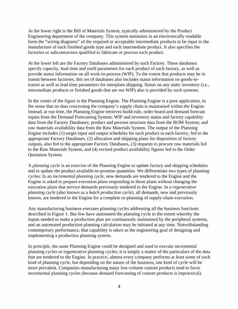
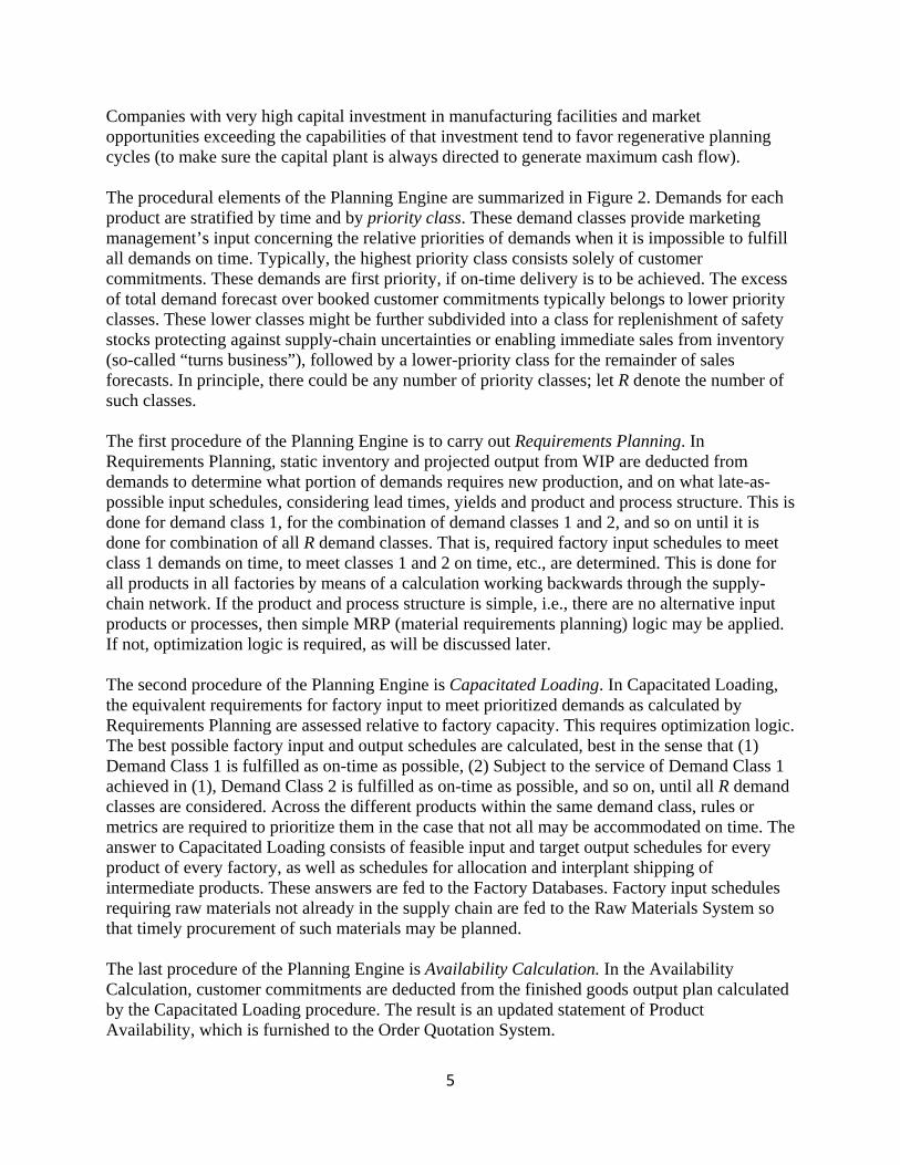
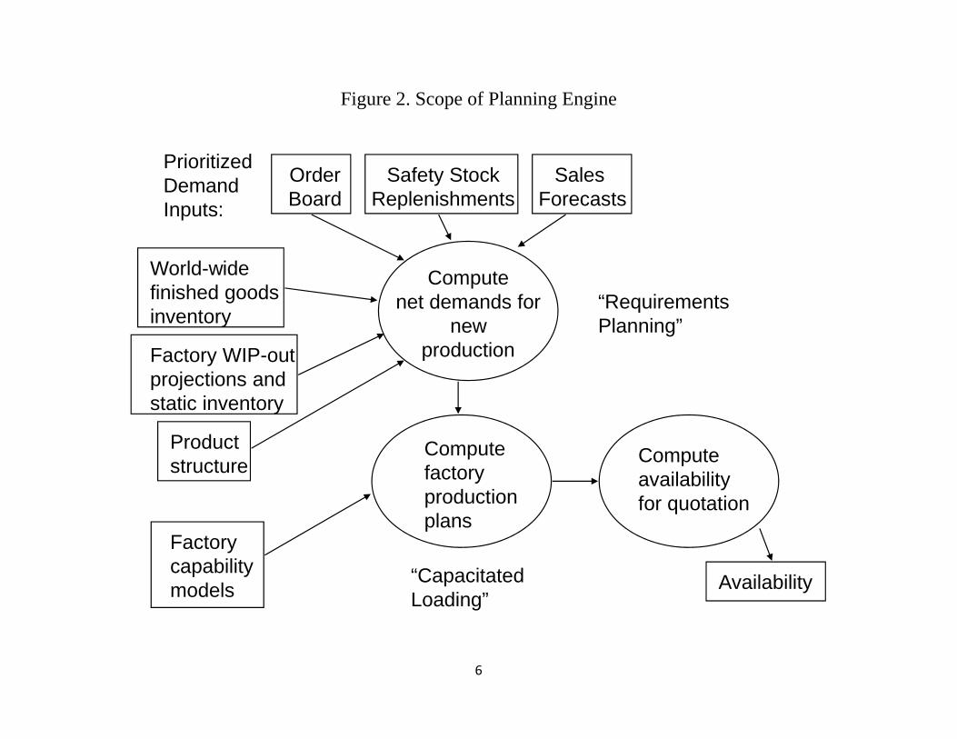
Companies with very high capital investment in manufacturing facilities and market opportunities exceeding the capabilities of that investment tend to favor regenerative planning cycles (to make sure the capital plant is always directed to generate maximum cash flow). The procedural elements of the Planning Engine are summarized in Figure 2. Demands for each product are stratified by time and by priority class. These demand classes provide marketing management’s input concerning the relative priorities of demands when it is impossible to fulfill all demands on time. Typically, the highest priority class consists solely of customer commitments. These demands are first priority, if on-time delivery is to be achieved. The excess of total demand forecast over booked customer commitments typically belongs to lower priority classes. These lower classes might be further subdivided into a class for replenishment of safety stocks protecting against supply-chain uncertainties or enabling immediate sales from inventory (so-called “turns business”), followed by a lower-priority class for the remainder of sales forecasts. In principle, there could be any number of priority classes; let R denote the number of such classes. The first procedure of the Planning Engine is to carry out Requirements Planning. In Requirements Planning, static inventory and projected output from WIP are deducted from demands to determine what portion of demands requires new production, and on what late-as-possible input schedules, considering lead times, yields and product and process structure. This is done for demand class 1, for the combination of demand classes 1 and 2, and so on until it is done for combination of all R demand classes. That is, required factory input schedules to meet class 1 demands on time, to meet classes 1 and 2 on time, etc., are determined. This is done for all products in all factories by means of a calculation working backwards through the supply-chain network. If the product and process structure is simple, i.e., there are no alternative input products or processes, then simple MRP (material requirements planning) logic may be applied. If not, optimization logic is required, as will be discussed later. The second procedure of the Planning Engine is Capacitated Loading. In Capacitated Loading, the equivalent requirements for factory input to meet prioritized demands as calculated by Requirements Planning are assessed relative to factory capacity. This requires optimization logic. The best possible factory input and output schedules are calculated, best in the sense that (1) Demand Class 1 is fulfilled as on-time as possible, (2) Subject to the service of Demand Class 1 achieved in (1), Demand Class 2 is fulfilled as on-time as possible, and so on, until all R demand classes are considered. Across the different products within the same demand class, rules or metrics are required to prioritize them in the case that not all may be accommodated on time. The answer to Capacitated Loading consists of feasible input and target output schedules for every product of every factory, as well as schedules for allocation and interplant shipping of intermediate products. These answers are fed to the Factory Databases. Factory input schedules requiring raw materials not already in the supply chain are fed to the Raw Materials System so that timely procurement of such materials may be planned. The last procedure of the Planning Engine is Availability Calculation. In the Availability Calculation, customer commitments are deducted from the finished goods output plan calculated by the Capacitated Loading procedure. The result is an updated statement of Product Availability, which is furnished to the Order Quotation System.
6
Figure 2. Scope of Planning Engine
PrioritizedDemandInputs:
OrderBoard
Safety StockReplenishments
Sales Forecasts
World-widefinished goodsinventory
Factory WIP-outprojections andstatic inventory
Productstructure
Computenet demands for
newproduction
Factorycapabilitymodels
Computefactoryproductionplans
Computeavailabilityfor quotation
Availability
“RequirementsPlanning”
“CapacitatedLoading”
7
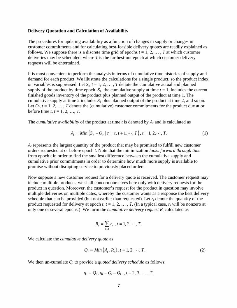
Delivery Quotation and Calculation of Availability The procedures for updating availability as a function of changes in supply or changes in customer commitments and for calculating best-feasible delivery quotes are readily explained as follows. We suppose there is a discrete time grid of epochs t = 1, 2, … , T at which customer deliveries may be scheduled, where T is the farthest-out epoch at which customer delivery requests will be entertained. It is most convenient to perform the analysis in terms of cumulative time histories of supply and demand for each product. We illustrate the calculations for a single product, so the product index on variables is suppressed. Let St, t = 1, 2, … , T denote the cumulative actual and planned supply of the product by time epoch. S1, the cumulative supply at time t = 1, includes the current finished goods inventory of the product plus planned output of the product at time 1. The cumulative supply at time 2 includes S1 plus planned output of the product at time 2, and so on. Let Ot, t = 1, 2, … , T denote the (cumulative) customer commitments for the product due at or before time t, t = 1, 2, …, T. The cumulative availability of the product at time t is denoted by At and is calculated as
.,,2,1,,,1,| TtTttOSMinAt (1)
At represents the largest quantity of the product that may be promised to fulfill new customer orders requested at or before epoch t. Note that the minimization looks forward through time from epoch t in order to find the smallest difference between the cumulative supply and cumulative prior commitments in order to determine how much more supply is available to promise without disrupting service to previously placed orders. Now suppose a new customer request for a delivery quote is received. The customer request may include multiple products; we shall concern ourselves here only with delivery requests for the product in question. Moreover, the customer’s request for the product in question may involve multiple deliveries on multiple dates, whereby the customer wants as a response the best delivery schedule that can be provided (but not earlier than requested). Let rt denote the quantity of the product requested for delivery at epoch t, t = 1, 2, … , T. (In a typical case, rt will be nonzero at only one or several epochs.) We form the cumulative delivery request Rt calculated as
.,,2,1,1
TtrRt
t
We calculate the cumulative delivery quote as
.,,2,1,, TtRAMinQ ttt (2)
We then un-cumulate Qt to provide a quoted delivery schedule as follows:
q1 = Q1, qt = Qt – Qt-1, t = 2, 3, … , T,

8
and we update the cumulative availability as follows:
.,,2,1,,,1,| TtTttQAMinAt (3)
We also should update the order board to (tentatively) include a reservation for the customer reflecting the quote provided, i.e.,
.,,2,1, TtQOO ttt
If the customer rejects the quote or if the quote expires without the customer committing an order, then the cumulative quote Qt should be deleted from the cumulative orders Ot, i.e.,
,,,2,1, TtQOO ttt
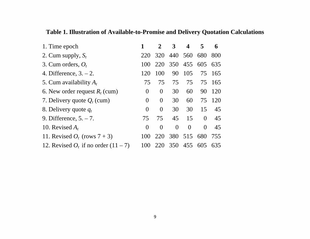
whereupon the cumulative availability should be recalculated as in (1). Numerical Example We illustrate the foregoing formulas with the numerical example in Table 1. Suppose for a particular product the finished goods inventory level is 120. The planned supply is 100 at epoch 1, 100 at epoch 2, 120 at epoch 3, 120 at epoch 4, 120 at epoch 5, and 120 at epoch 6. This results in the cumulative supply schedule shown in row 2 of the table. Suppose the delivery schedules for previously accepted orders amount to 100 at epoch 1, 120 at epoch 2, 130 at epoch 3, 105 at epoch 4, 150 at epoch 5, and 30 at epoch 6. This results in the cumulative orders schedule shown in row 3 of the table. Row 4 simply differences these two time histories. Row 5 applies the Min formula to establish the cumulative availability at each epoch. At or before epoch 5, not more than 75 can be promised to prospective customers, after which the availability rises to 165. Finally, suppose a customer request for a quote is received requesting deliveries of 30 units at each of epochs 3, 4, 5 and 6. This results in the cumulative order request shown in row 6 of the table. Taking a Min with row 5 (the cumulative availability) results in the cumulative delivery quote shown in row 7. This quote is un-cumulated in row 8. As shown in row 8, the company’s best response to the customer’s inquiry is to offer 30 units at epochs 3 and 4, but drop to only 15 units supplied at epoch 5, but then recover and deliver 45 units at epoch 6. Row 9 differences row 5 (the cumulative availability) and row 7 (the cumulative quote). In row 10 the Min formula is applied to update the availability. In row 11 the cumulative orders are updated to (tentatively) include the cumulative quote. Should the customer reject the quote or should the quote expire, then a transaction is required to delete the quote from the orders. This is done in row 12. Immediately following that transaction there should be another transaction to restore the availability. This is done by repeating the calculations in rows 4 and 5.
9
Table 1. Illustration of Available-to-Promise and Delivery Quotation Calculations
1. Time epoch 1 2 3 4 5 6
2. Cum supply, St 220 320 440 560 680 800
3. Cum orders, Ot 100 220 350 455 605 635
4. Difference, 3. – 2. 120 100 90 105 75 165
5. Cum availability At 75 75 75 75 75 165
6. New order request Rt (cum) 0 0 30 60 90 120
7. Delivery quote Qt (cum) 0 0 30 60 75 120
8. Delivery quote qt 0 0 30 30 15 45
9. Difference, 5. – 7. 75 75 45 15 0 45
10. Revised At 0 0 0 0 0 45
11. Revised Ot (rows 7 + 3) 100 220 380 515 680 755
12. Revised Ot if no order (11 – 7) 100 220 350 455 605 635
10
Requirements Planning The standard calculus for computing material requirements, i.e., translating end-item demands into requirements for production of components and ordering of raw materials, is widely known and widely available in software. (Hereafter, this calculus is termed “the MRP calculus.”) Certain restrictive assumptions about the product structure are required for the MRP calculus to be applicable:
- For any product, there are no alternatives for each of its predecessor components, i.e., there cannot be any choice of components to input for the production of the given product.
- For any product, there cannot be a choice of manufacturing facilities to manufacture the
product, i.e., the manufacturing source for the product is unique. If either of these conditions is not met, MRP calculus must be supplemented with other logic to decide among alternative sources. An additional concern is related to economics. Some product structures are characterized by binning and substitution. For example, testing of a manufacturing lot may categorize product units within the batch into various grades of quality or bins. The average fraction of manufacturing output ending up in a certain bin of quality is termed the bin split for that bin. A follow-on product or customer sale may require a particular bin of quality or may accept any of several bins of quality. In such a case, it may be unprofitable to accept all demands for low-bin-split items. If such demands were accepted, it would entail excessive production and excessive supply of the other bins, far exceeding their demand. If economics is a concern, the MRP calculus must be supplemented with other logic to decide whether or not to accept demands and propagate the demands as material requirements.
Requirements plans are most commonly prepared in terms of event-based schedules, i.e., quantities to input or ship or procure by date. For repetitive volume manufacturing, an alternative means of expressing plans is in terms of rate-based schedules. In rate-based schedules, a time grid of epochs is specified. Between consecutive epochs, the rates of material flows input into manufacturing processes are required or assumed to be held constant. If we label the interval (t-1, t] as “period t”, a decision variable xt indicates the rate of material flow scheduled during period t. Software intended to generate event-based material requirements plans will schedule material quantities at specific delivery times, i.e., xt denotes the quantity of the material to be delivered at epoch t. The software may be used to generate rate-based schedules if the decision variable xt is interpreted as the rate of flow during (t-1, t] rather than the quantity due or occurring at epoch t. A challenge arises if rates of flow are desired to be held constant during relatively long periods such as weeks. In that case, the need for lead times to be integer in the MRP calculus presents a problem. Fortunately, the MRP calculus can be revised to admit non-integer lead times while generating rate-based schedules expressing constant rates of material flow in the given intervals.

11
Capacitated Loading Once new production requirements are determined, the next phase of the planning cycle concerns loading such requirements on factories in a feasible schedule of launches for production lots and the consequent target output schedules. Process-based industries, such as petroleum refining, paper making, aluminum making or the like, have since the 1950s employed linear programming optimization calculations to make capacitated loading decisions. Such industries are characterized by a very capital-intensive resource carrying out continuous or near-continuous production governed by rate-based schedules. For such industries, linear programming or mixed integer linear programming is a very good fit. Industries characterized by many stages of fabrication and assembly of many different kinds of discrete parts in low-volumes or infrequent batches are much less amenable to accurate, practical modeling under the linear programming paradigm. Considering the large numbers of products and inventory points involved, a precise mathematical programming model becomes impractically large. In such industries the application of LP is rare. Instead, it is more common for approximate capacity analyses to be carried out using spreadsheets making calculations of approximate workloads on artificial, aggregate resources or some subset of important resources. Results of such spreadsheet analyses are the subject of discussion, review and iteration, and, as a result, planning cycles are rarely automated in such industries. The semiconductor industry straddles the boundary between discrete parts manufacturing and process industry. Discrete manufacturing lots are progressed through many process steps in fabrication, assembly and testing, yet fabrication plants are extremely capital-intensive. The number of levels in the product structure is relatively small, and production volumes of products, or of families of products with similar capacity consumption, are high. Thus the numbers of inventory points and products for capacity analysis are relatively low, rendering the capacitated loading problem amenable to LP optimization. A special challenge presented by semiconductor manufacturing, and, for that matter, by all industries utilizing planar fabrication process technology, is that the manufacturing process flows are re-entrant. In wafer fabrication, multiple layers of circuitry are built up on the wafers, necessitating repeated visits to equipment interspersed with visits to other equipment. This means new production lots must compete with work-in-process for capacity. Workloads on resources become functions of the time-histories of production lot launches. Considerable sophistication is required to generate an accurate yet practical linear programming formulation, as will be discussed below. Product Structure and Inventory vs. WIP In general, there are choices that can be made when defining product and process structures and when establishing inventory points to de-couple manufacturing stages. Amenability of the planning problem to formal optimization is seldom a criterion for consideration when such structures are defined. But it is an important consideration, as successful application of formal

12
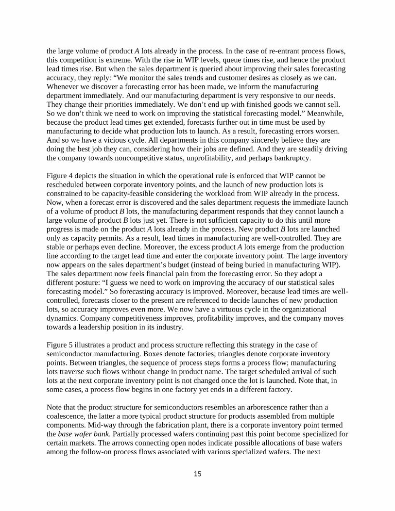
optimization enables much faster and more frequent planning cycles to be performed. To minimize the number of inventory points, the following rule is suggested: 1. If the next processing step does not require input of major raw materials or other products, and the next step does not reduce the potential market for the product, then the product name should not change at the next step and there should not be an inventory point before the next step. To understand this rule, note that portions of the overall manufacturing process may consist of series of processing steps in which no assembly or co-production occurs, and the product under production is not completed until the end of the series. The sequence of steps in the series is termed a process flow. A manufacturing lot of a given product passes through such a process flow without changing levels in the product structure. If at a certain step the potential market for the lot is reduced, this means specialized processing is being performed to render the product suitable for a certain subset of potential customers. A different choice of specialized processing on the manufacturing lot would make it suitable for a different subset of customers. This choice necessitates a change of levels in the product structure, i.e., a change of product names. It may be desirable to hold an inventory before the specialization point, especially if the build rules entail building to plan before specialization and building to order afterwards. In this case, a corporate inventory point is defined just in front of the first specialization processing step. In typical practice, other inventory points may arise for administrative or jurisdictional convenience, permitting asynchronous scheduling of steps before and after such a point. These inventories are unnecessary from a production planning point of view. As a complement to the product and process structure as defined by rule 1 above, the following operational rule is suggested: 2. Production activity between corporate inventory points is organized into process flows operated with rate-based schedules. Once production lots are launched into a process flow, they are not eligible for re-scheduling until they reach the next corporate inventory point. That is, such lots must be kept moving according to target lead times. Moreover, production lots are scheduled to leave corporate inventory points only if workload and capacity permit progressing the lots to the next corporate inventory point according to rate-based scheduling and target lead times. The rationale for this rule is illustrated in Figures 3 and 4. Figure 3 illustrates the case where rule 2 is not enforced. A vicious cycle arises in the organizational dynamics. We could start the explanation of this cycle at any point, but let us start in the upper left, where the sales department generates forecasts for the various products and informs manufacturing, which launches production lots accordingly. Now suppose the sales department discovers a major forecasting error; it turns out that customers actually prefer product B over product A, but the forecast had predicted strong sales of product A. The sales department calls the manufacturing department immediately upon learning of the error and asks manufacturing to de-prioritize the large volume of lots of product A in process, and instead please hurry and launch a large volume of lots of product B. Manufacturing management complies. But manufacturing management cannot eliminate competition for capacity between the large volume of product B lots just launched and

13
Figure 3. Vicious Cycle in Organizational Dynamics When WIP is Re-Scheduled
IncreasingSalesForecastError
Manufacturingreprioritizes WIP
Lead time gets longer
Since Manufacturingcompensated for error,Sales dept. feels no needto improve forecasting
14
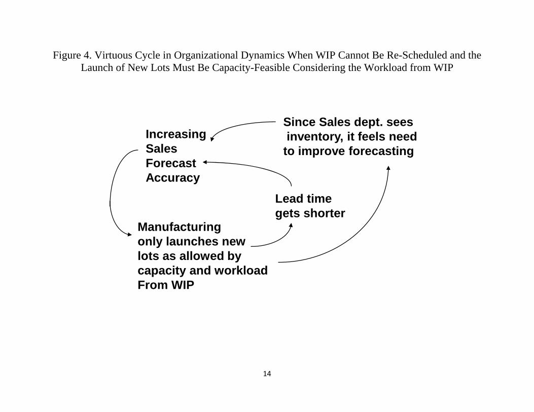
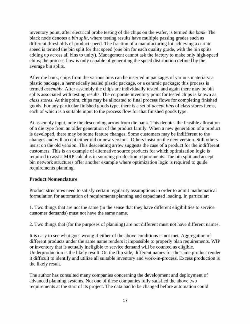
Figure 4. Virtuous Cycle in Organizational Dynamics When WIP Cannot Be Re-Scheduled and the Launch of New Lots Must Be Capacity-Feasible Considering the Workload from WIP
IncreasingSalesForecastAccuracy
Manufacturingonly launches newlots as allowed by capacity and workloadFrom WIP
Lead time gets shorter
Since Sales dept. sees inventory, it feels need
to improve forecasting
15
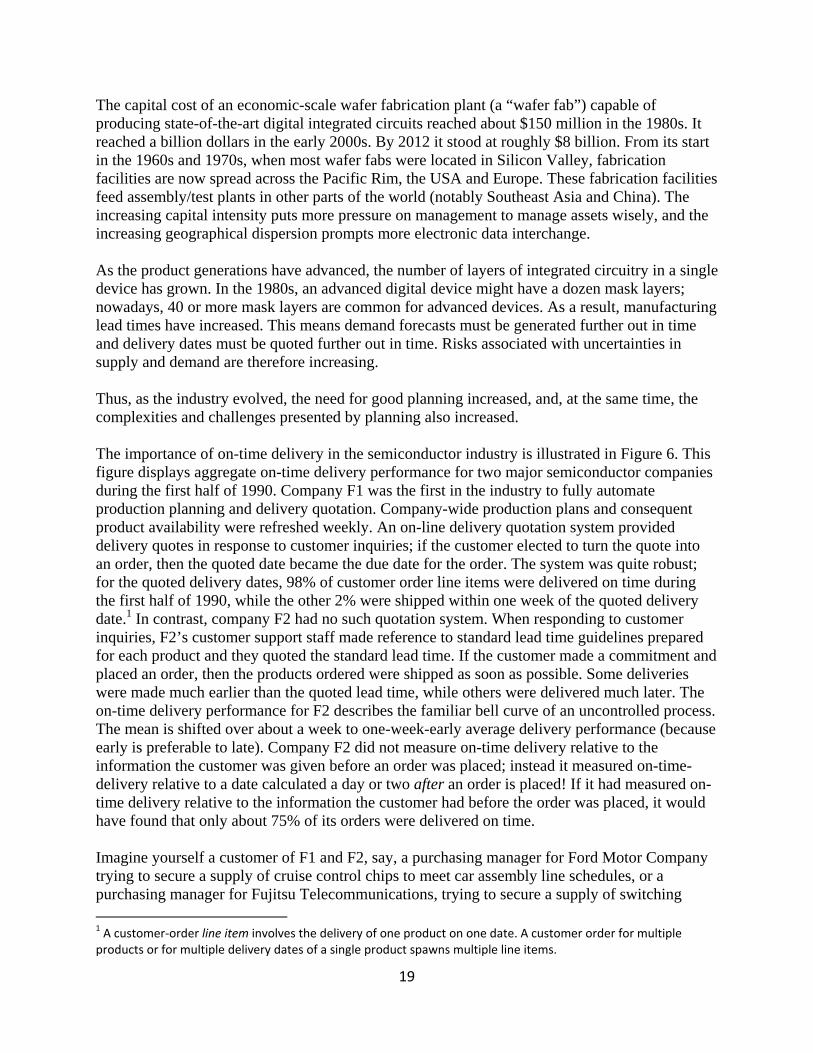
the large volume of product A lots already in the process. In the case of re-entrant process flows, this competition is extreme. With the rise in WIP levels, queue times rise, and hence the product lead times rise. But when the sales department is queried about improving their sales forecasting accuracy, they reply: “We monitor the sales trends and customer desires as closely as we can. Whenever we discover a forecasting error has been made, we inform the manufacturing department immediately. And our manufacturing department is very responsive to our needs. They change their priorities immediately. We don’t end up with finished goods we cannot sell. So we don’t think we need to work on improving the statistical forecasting model.” Meanwhile, because the product lead times get extended, forecasts further out in time must be used by manufacturing to decide what production lots to launch. As a result, forecasting errors worsen. And so we have a vicious cycle. All departments in this company sincerely believe they are doing the best job they can, considering how their jobs are defined. And they are steadily driving the company towards noncompetitive status, unprofitability, and perhaps bankruptcy. Figure 4 depicts the situation in which the operational rule is enforced that WIP cannot be rescheduled between corporate inventory points, and the launch of new production lots is constrained to be capacity-feasible considering the workload from WIP already in the process. Now, when a forecast error is discovered and the sales department requests the immediate launch of a volume of product B lots, the manufacturing department responds that they cannot launch a large volume of product B lots just yet. There is not sufficient capacity to do this until more progress is made on the product A lots already in the process. New product B lots are launched only as capacity permits. As a result, lead times in manufacturing are well-controlled. They are stable or perhaps even decline. Moreover, the excess product A lots emerge from the production line according to the target lead time and enter the corporate inventory point. The large inventory now appears on the sales department’s budget (instead of being buried in manufacturing WIP). The sales department now feels financial pain from the forecasting error. So they adopt a different posture: “I guess we need to work on improving the accuracy of our statistical sales forecasting model.” So forecasting accuracy is improved. Moreover, because lead times are well-controlled, forecasts closer to the present are referenced to decide launches of new production lots, so accuracy improves even more. We now have a virtuous cycle in the organizational dynamics. Company competitiveness improves, profitability improves, and the company moves towards a leadership position in its industry. Figure 5 illustrates a product and process structure reflecting this strategy in the case of semiconductor manufacturing. Boxes denote factories; triangles denote corporate inventory points. Between triangles, the sequence of process steps forms a process flow; manufacturing lots traverse such flows without change in product name. The target scheduled arrival of such lots at the next corporate inventory point is not changed once the lot is launched. Note that, in some cases, a process flow begins in one factory yet ends in a different factory. Note that the product structure for semiconductors resembles an arborescence rather than a coalescence, the latter a more typical product structure for products assembled from multiple components. Mid-way through the fabrication plant, there is a corporate inventory point termed the base wafer bank. Partially processed wafers continuing past this point become specialized for certain markets. The arrows connecting open nodes indicate possible allocations of base wafers among the follow-on process flows associated with various specialized wafers. The next

16
Die Bank
Bin Inventory
Assem- bly
Initial Test
Brand, Re-Test
& Pack
Packaged Device Finished
Goods
Wafer Fab
Probe
DieWaferBase
Wafer
Finished Goods
Standardized Representation of the Product and Process
Structure Within BPS
Bins
Wafer Bank
Wafer Fab
Figure 5. Product and Process Structure for Semiconductor Manufacturing
17
inventory point, after electrical probe testing of the chips on the wafer, is termed die bank. The black node denotes a bin split, where testing results have multiple passing grades such as different thresholds of product speed. The fraction of a manufacturing lot achieving a certain speed is termed the bin split for that speed (one bin for each quality grade, with the bin splits adding up across all bins to unity). Management cannot ask the factory to make only high-speed chips; the process flow is only capable of generating the speed distribution defined by the average bin splits. After die bank, chips from the various bins can be inserted in packages of various materials: a plastic package, a hermetically sealed plastic package, or a ceramic package; this process is termed assembly. After assembly the chips are individually tested, and again there may be bin splits associated with testing results. The corporate inventory point for tested chips is known as class stores. At this point, chips may be allocated to final process flows for completing finished goods. For any particular finished goods type, there is a set of accept bins of class stores items, each of which is a suitable input to the process flow for that finished goods type. At assembly input, note the descending arrow from die bank. This denotes the feasible allocation of a die type from an older generation of the product family. When a new generation of a product is developed, there may be some feature changes. Some customers may be indifferent to the changes and will accept either old or new versions. Others insist on the new version. Still others insist on the old version. This descending arrow suggests the case of a product for the indifferent customers. This is an example of alternative source products for which optimization logic is required to assist MRP calculus in sourcing production requirements. The bin split and accept bin network structures offer another example where optimization logic is required to guide requirements planning. Product Nomenclature Product structures need to satisfy certain regularity assumptions in order to admit mathematical formulation for automation of requirements planning and capacitated loading. In particular: 1. Two things that are not the same (in the sense that they have different eligibilities to service customer demands) must not have the same name. 2. Two things that (for the purposes of planning) are not different must not have different names. It is easy to see what goes wrong if either of the above conditions is not met. Aggregation of different products under the same name renders it impossible to properly plan requirements. WIP or inventory that is actually ineligible to service demand will be counted as eligible. Underproduction is the likely result. On the flip side, different names for the same product render it difficult to identify and utilize all suitable inventory and work-in-process. Excess production is the likely result. The author has consulted many companies concerning the development and deployment of advanced planning systems. Not one of these companies fully satisfied the above two requirements at the start of its project. The data had to be changed before automation could

18
proceed. For this reason, these two requirements have become known as “Leachman’s Laws of Nomenclature.” A Specific Planning Challenge: Semiconductor Manufacturing Any industry founded on the basis of new technology passes through a competitive evolution. At the beginning, a single company may possess a proprietary technology and be the sole source for products enabled by the technology. Competition in this early phase is generally characterized by efforts to get prospective customers to adopt the revolutionary products as components of their own products or for use in their business or personal lives. Sooner or later competitors will arise, either competitors using the same technology (because the technology has been licensed or because the patents have expired), or competitors utilizing alternative technologies to generate comparable products. Competition on the basis of price ensues. If the technology is accepted such that new products are immediately valued in the marketplace, the competition on the basis of speed of development and speed of delivery also arises. And finally, if the products are themselves components of larger system products, then the ability to deliver orders at requested or promised delivery dates becomes a basis for competition. This basis arises because later deliveries delay the completion of the system-level products or increase costs of the client companies by impelling them to maintain expensive safety stocks of components. As this competitive evolution unfolds, the ability to control and direct the manufacturing network becomes more and more important. This control is needed to achieve lowest possible cost (price competition), fastest possible speed (speed competition), and most reliable delivery (on-time delivery competition). The foregoing description certainly characterizes the competitive evolution of the semiconductor industry. In parallel with the evolution of competition, the challenge presented by the task of controlling and directing the manufacturing network became steadily more formidable. Moore’s Law refers to the rapid pace of technological progress in the industry, whereby the dimensions of an electrical switch, transistor or memory cell are shrunk 50% every 1.5-3 years. Historically speaking and roughly speaking, this enabled either a 50% cost reduction or a 50% product capability improvement every couple of years. The flip side of Moore’s Law is Rock’s Law, named after Arthur Rock, and early venture capitalist in Silicon Valley. Rock quipped to Gordon Moore (an Intel executive), “Gordon, that’s great that you have such a rapid pace of technological improvement, but I notice that every time you ask me for money for a new factory, you ask for twice as much.” Each product generation (“shrink”) requires more sophisticated silicon wafer processing equipment. The unit cost of equipment keeps rising, but the output (if measured in switches or memory cells) per equipment rises even more. Similarly, the unit cost of engineering staff to manage the factory keeps rising (because of the increased sophistication of process and equipment they must engineer and manage), but not as much as the output per engineer rises. The rising unit costs of equipment and staff drive the economic scale of factories ever higher (to mitigate the percentage costs of rounding up equipment and engineer staff requirements to the next integer number of machines or engineers). This in turn means the stakes involved in planning are aver higher.
19
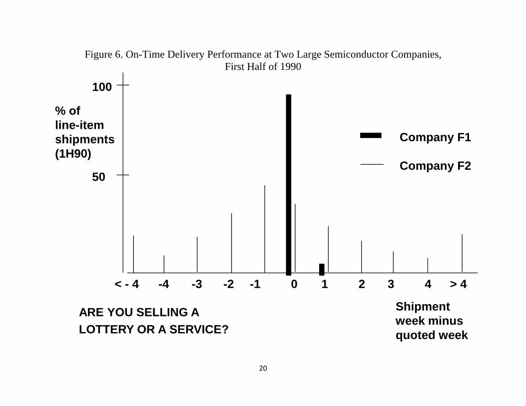
The capital cost of an economic-scale wafer fabrication plant (a “wafer fab”) capable of producing state-of-the-art digital integrated circuits reached about $150 million in the 1980s. It reached a billion dollars in the early 2000s. By 2012 it stood at roughly $8 billion. From its start in the 1960s and 1970s, when most wafer fabs were located in Silicon Valley, fabrication facilities are now spread across the Pacific Rim, the USA and Europe. These fabrication facilities feed assembly/test plants in other parts of the world (notably Southeast Asia and China). The increasing capital intensity puts more pressure on management to manage assets wisely, and the increasing geographical dispersion prompts more electronic data interchange. As the product generations have advanced, the number of layers of integrated circuitry in a single device has grown. In the 1980s, an advanced digital device might have a dozen mask layers; nowadays, 40 or more mask layers are common for advanced devices. As a result, manufacturing lead times have increased. This means demand forecasts must be generated further out in time and delivery dates must be quoted further out in time. Risks associated with uncertainties in supply and demand are therefore increasing. Thus, as the industry evolved, the need for good planning increased, and, at the same time, the complexities and challenges presented by planning also increased. The importance of on-time delivery in the semiconductor industry is illustrated in Figure 6. This figure displays aggregate on-time delivery performance for two major semiconductor companies during the first half of 1990. Company F1 was the first in the industry to fully automate production planning and delivery quotation. Company-wide production plans and consequent product availability were refreshed weekly. An on-line delivery quotation system provided delivery quotes in response to customer inquiries; if the customer elected to turn the quote into an order, then the quoted date became the due date for the order. The system was quite robust; for the quoted delivery dates, 98% of customer order line items were delivered on time during the first half of 1990, while the other 2% were shipped within one week of the quoted delivery date.1 In contrast, company F2 had no such quotation system. When responding to customer inquiries, F2’s customer support staff made reference to standard lead time guidelines prepared for each product and they quoted the standard lead time. If the customer made a commitment and placed an order, then the products ordered were shipped as soon as possible. Some deliveries were made much earlier than the quoted lead time, while others were delivered much later. The on-time delivery performance for F2 describes the familiar bell curve of an uncontrolled process. The mean is shifted over about a week to one-week-early average delivery performance (because early is preferable to late). Company F2 did not measure on-time delivery relative to the information the customer was given before an order was placed; instead it measured on-time-delivery relative to a date calculated a day or two after an order is placed! If it had measured on-time delivery relative to the information the customer had before the order was placed, it would have found that only about 75% of its orders were delivered on time. Imagine yourself a customer of F1 and F2, say, a purchasing manager for Ford Motor Company trying to secure a supply of cruise control chips to meet car assembly line schedules, or a purchasing manager for Fujitsu Telecommunications, trying to secure a supply of switching 1 A customer‐order line item involves the delivery of one product on one date. A customer order for multiple products or for multiple delivery dates of a single product spawns multiple line items.
20
Figure 6. On-Time Delivery Performance at Two Large Semiconductor Companies, First Half of 1990
100
0 1 2 3 4 > 4-1-2-3-4< - 4
Shipmentweek minusquoted week
% ofline-itemshipments(1H90)
50
Company F1
Company F2
ARE YOU SELLING ALOTTERY OR A SERVICE?
21
network controller chips to meet schedules for installation of communication networks. Who would you rather do business with? Company F1 provides pretty reliable delivery quotations; little risk is taken doing business with them. Only modest safety stock is required to protect against late deliveries. Doing business with Company F2 presents a major headache; the chips might arrive way ahead of when needed, or they might be very late in arriving. Major safety stocks are required to use them as a supplier; and despite that, the prospect of excess inventories of their components is high. You might even be willing to pay company F1 a premium to do business with it; it sells a service, whereas F1 sells a lottery. If you were forced to do business with F2 as a supplier, what would you do? You cannot risk shutting down the assembly lines in your own company. You would likely order components before you really needed them, and/or you would ask for more than you really needed. We can see how the lack of good information provided by F2 to its customers is likely to generate much turbulence in the supply chain, especially at times when customers perceive that supply will be tight (e.g., new product introductions or economic boom periods. Because of its inferior on-time delivery performance, company F2 nearly went bankrupt. Its sales were declining more than $100 million per year. With the author’s help, F2 implemented advanced production planning and delivery quotation systems, and ultimately achieved outstanding delivery performance and considerable financial success. In contrast, some weaknesses in F1’s systems emerged. It automatically accepted all customer requests more than six months out. Unfortunately, during the economic boom in the second half of 1990, F1’s production capacity available to certain product families became saturated. Late deliveries became more prevalent in the second half of 1990, whereupon F1’s on-time delivery performance slipped to 93%. The Grand Challenges Presented by Planning Semiconductor Production Under the sponsorship of many semiconductor companies, the author undertook research 1983-1990 to develop an advanced but practical production planning engine for the semiconductor industry. Then during 1990-91, the author took a year’s leave of absence from the University of California to lead a project at the Semiconductor Sector of Harris Corporation to develop and implement automated planning and delivery quotation system. This system was known at Harris as IMPReSS (an acronym standing for Integrated Production Requirements Scheduling System). In retrospect, the major challenges that had to be faced and overcome in the IMPReSS project were as follows:
- Evolving to a standardized product and process structure with only four corporate inventory points in the product structure.
- Efficiently accomplishing requirements planning through product structures with binning and alternative source products.
- Capacity analysis of re-entrant process flows. - Incorporating marketing strategy and policies into production plan generation. - Coping with an immense problem scale. Delivery quotation was required over a horizon
of 1.5 years on a product catalog with 10,000 items. - Organizational change necessary to support and accept automated planning.
22
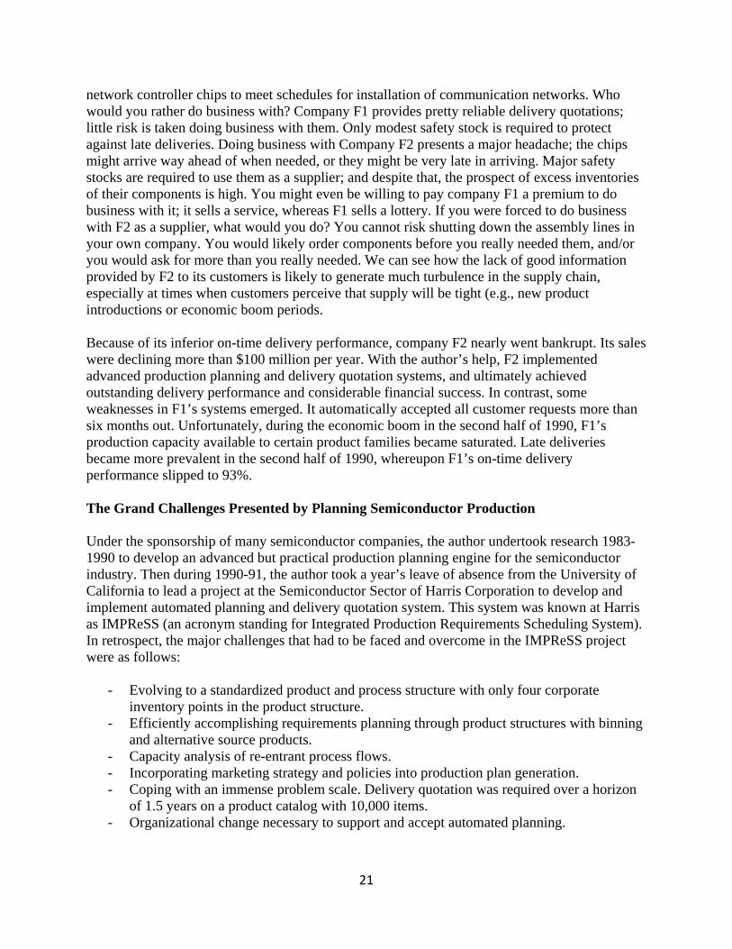
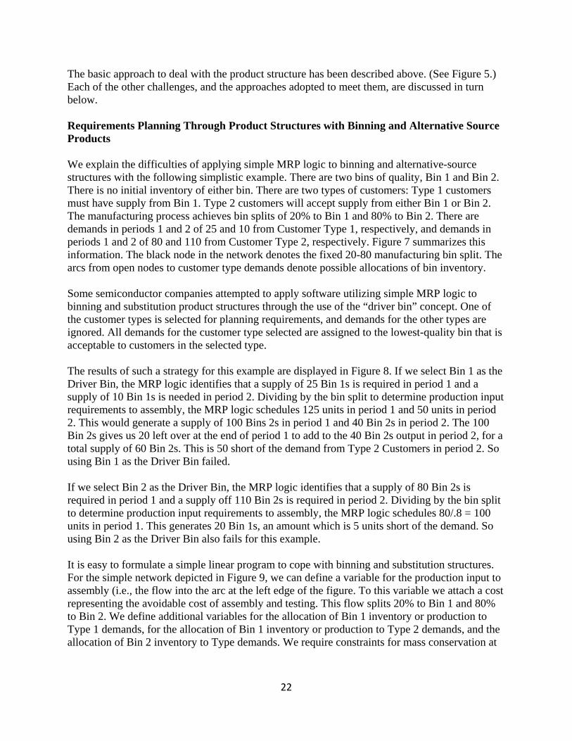
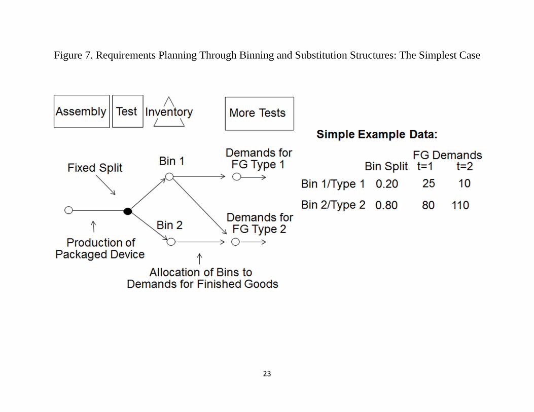
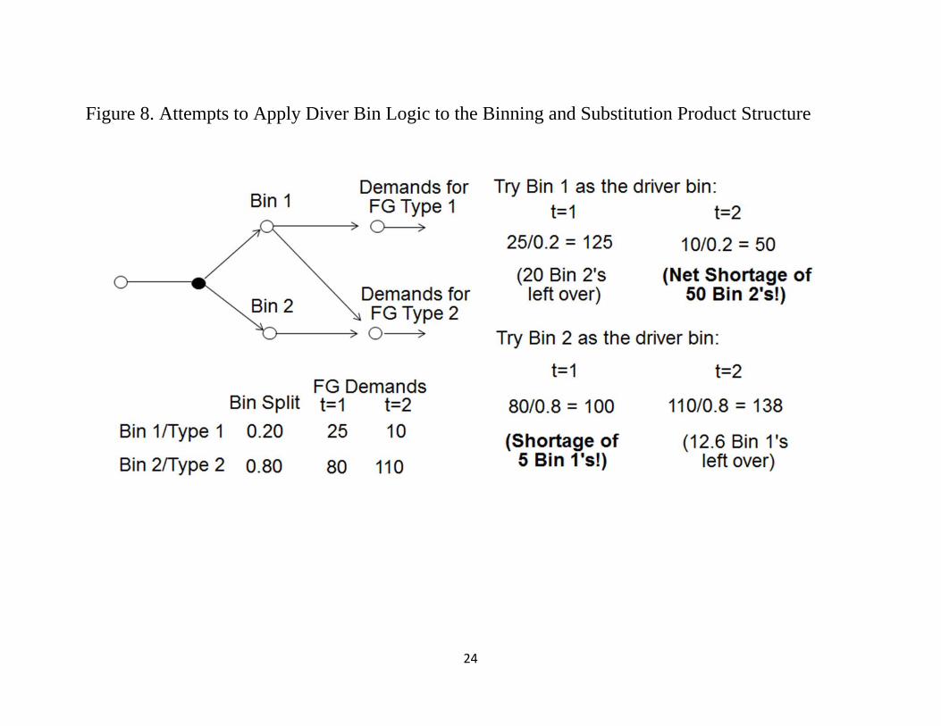
The basic approach to deal with the product structure has been described above. (See Figure 5.) Each of the other challenges, and the approaches adopted to meet them, are discussed in turn below. Requirements Planning Through Product Structures with Binning and Alternative Source Products We explain the difficulties of applying simple MRP logic to binning and alternative-source structures with the following simplistic example. There are two bins of quality, Bin 1 and Bin 2. There is no initial inventory of either bin. There are two types of customers: Type 1 customers must have supply from Bin 1. Type 2 customers will accept supply from either Bin 1 or Bin 2. The manufacturing process achieves bin splits of 20% to Bin 1 and 80% to Bin 2. There are demands in periods 1 and 2 of 25 and 10 from Customer Type 1, respectively, and demands in periods 1 and 2 of 80 and 110 from Customer Type 2, respectively. Figure 7 summarizes this information. The black node in the network denotes the fixed 20-80 manufacturing bin split. The arcs from open nodes to customer type demands denote possible allocations of bin inventory. Some semiconductor companies attempted to apply software utilizing simple MRP logic to binning and substitution product structures through the use of the “driver bin” concept. One of the customer types is selected for planning requirements, and demands for the other types are ignored. All demands for the customer type selected are assigned to the lowest-quality bin that is acceptable to customers in the selected type. The results of such a strategy for this example are displayed in Figure 8. If we select Bin 1 as the Driver Bin, the MRP logic identifies that a supply of 25 Bin 1s is required in period 1 and a supply of 10 Bin 1s is needed in period 2. Dividing by the bin split to determine production input requirements to assembly, the MRP logic schedules 125 units in period 1 and 50 units in period 2. This would generate a supply of 100 Bins 2s in period 1 and 40 Bin 2s in period 2. The 100 Bin 2s gives us 20 left over at the end of period 1 to add to the 40 Bin 2s output in period 2, for a total supply of 60 Bin 2s. This is 50 short of the demand from Type 2 Customers in period 2. So using Bin 1 as the Driver Bin failed. If we select Bin 2 as the Driver Bin, the MRP logic identifies that a supply of 80 Bin 2s is required in period 1 and a supply off 110 Bin 2s is required in period 2. Dividing by the bin split to determine production input requirements to assembly, the MRP logic schedules 80/.8 = 100 units in period 1. This generates 20 Bin 1s, an amount which is 5 units short of the demand. So using Bin 2 as the Driver Bin also fails for this example. It is easy to formulate a simple linear program to cope with binning and substitution structures. For the simple network depicted in Figure 9, we can define a variable for the production input to assembly (i.e., the flow into the arc at the left edge of the figure. To this variable we attach a cost representing the avoidable cost of assembly and testing. This flow splits 20% to Bin 1 and 80% to Bin 2. We define additional variables for the allocation of Bin 1 inventory or production to Type 1 demands, for the allocation of Bin 1 inventory or production to Type 2 demands, and the allocation of Bin 2 inventory to Type demands. We require constraints for mass conservation at
23
Figure 7. Requirements Planning Through Binning and Substitution Structures: The Simplest Case
24
Figure 8. Attempts to Apply Diver Bin Logic to the Binning and Substitution Product Structure

25
Figure 9. Network Underlying Linear Programming Formulation of Requirements Planning Through Binning Structures

26
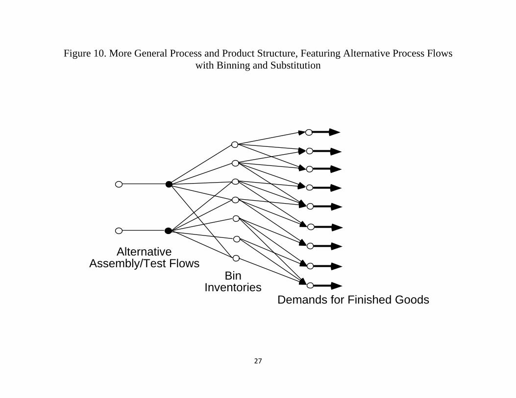
each of the bin inventory nodes and at each of the demand nodes. If there was only one period in the planning problem, that would the extent of the formulation. If there are additional periods, imagine repeating the same network for each time period. Between the network for period t and the network for period t+1, we add arcs between corresponding bin inventory nodes. Variables defined corresponding to these arcs represented holding inventory of bins from one period to the next and should be assigned an inventory cost. Alternatively, we could simply discount production costs on the assembly input arcs, whereby input in period t+1 is made cheaper than input in period t. We could then minimize the total discounted production cost to meet demands for all types in all periods. The result of the linear program would be equivalent assembly input requirements to the given demands for output by customer type. It is easy to extend this formulation to more general network structures. Figure 10 displays the case of alternative assembly/test flows providing different binning patterns. This would be the case if defining certain bins required additional tests (e.g., hot or cold temperature tests to define bins corresponding to device performance speed at hot or cold temperatures). As depicted in Figure 10, the relationship between bins of quality and customer demand types is, in general, a many-to-many relationship. If the process flows involving additional processing are assigned a higher cost, then a linear program formulated to minimize discounted production cost subject to meeting all demands will develop requirements plans that meet all demands as late as possible (but still on time) with minimum expenditures on testing. Generating the formulation is a simple matter of reading the product structure at run time, formulating variables for production input to each flow, formulating variables for allocation to each customer type of each of its accept bins, and enforcing constraints for mass conservation of bin inventories and customer type demands. However, in some instances, it is unwise to meet all demands. Returning to the simplest example, suppose the bin split to Bin 1 was 1%, but the Customer Type 1 demand was 1,000 times larger than the Customer Type 2 demand. Satisfying the Customer Type 1 demand would entail massive production levels and massive excess inventories of Bin 2. This could possibly cost more than the revenue obtained from the Type 1 demands. If some or all of the demands were forecasts but not yet customer orders, it could be unwise and unprofitable to create a large availability of finished goods for Type 1 customers unless there is an even larger Type 2 market available. Figure 11 illustrates the general behavior as assembly production volume is ramped up in response to forecasted demands. Starting from zero supply, low production levels generate supplies in various bins according to the bin splits, but if demands for every Customer Type materialize, then supplies may be fully allocated and maximum marginal revenue from production is realized. As production is ramped up, eventually demands in one or more Customer Types becomes saturated. At that point, some options for allocating bins to demands disappear, and so marginal revenue declines. The cumulative revenue follows a piecewise linear curve with declining slope, whereas production cost follows an increasing linear slope. Eventually, the slope of thee marginal revenue curve will fall below the production cost slope. At this point, no more supply should be generated, as the cost of further supply exceeds the revenue available from it. It is easy to adapt the linear programming formulation for this case. The objective function should include both positive and negative cash flows, with revenue assigned to bin allocation arcs and cost assigned to arcs representing production input to process flows. For a maximum discounted cash flow objective, the LP will plan supply only up to the level of profitability.
27
Figure 10. More General Process and Product Structure, Featuring Alternative Process Flows with Binning and Substitution
Most general product structure
Alternative Assembly/Test Flows
Bin Inventories
Demands for Finished Goods

28
Figure 11. Limiting Availability to Economic Levels
29
For the demand class structure introduced earlier, minimum-cost-objective LPs are used to plan requirements corresponding to customer-commitment and safety-stock replenishment demand classes, whereas maximum-profit-objective LPs are used to plan requirements corresponding to forecast demand classes (with appropriate consistency constraints ensuring supply to higher-priority classes is not disrupted). Consistency constraints are required to ensure the LP formulated to plan starts in response to demands in classes 1, 2, …, n does not undo starts calculated to plan starts responding to demands in classes 1, 2, …., n-1. Separate linear programming formulations may be prepared for product families with no common bins or demand types. In practice, requirements planning through binning and substitution structures involves solving many small linear programs that require modest computational time. Capacity Analysis and Capacitated Loading of Re-entrant Process Flows Most approaches to semiconductor capacity analysis assess the workloads from proposed fabrication input mix, tacitly assuming steady-state production in that mix. To illustrate the pitfalls of such an approach, consider the following simplistic example. Suppose the process flow to fabricate product P1 involves processing by machine type M1 in the first week, followed by processing using machine type M2 in the second week. Suppose the process flow to fabricate product P2 reverses this sequence, whereby machine type M2 is used in the first week and machine type M1 is used in the second week. Suppose the capacity of machine type M2 is 2,000 units per week of either product or any combination of the two products adding to 2,000 units. Now consider three alternative production plans: In Plan 1, it is proposed to input 2,000 units of product P1 in weeks 1 and 2, with no production of product P2. In Plan 2, it is proposed to input 2,000 units of product P2 in weeks 1 and 2, with no production of product P1. In Plan 3, it is proposed to input 2,000 units of product P1 in week 1, then input 2,000 units of product P2 in week 2. Plan 1 involves steady-state production of product P1 up to the capacity of M2; it is a feasible plan, at least as far as the capacity of M2 is concerned. Similarly, Plan 2 involves steady-state production of product P2 up to the capacity of M2; it also is a feasible plan. One might think that Plan 3 also presents a feasible plan, as it dynamically combines two steady-state production mixes that are feasible. It does not input any more than 2,000 units per week, so it might seem to be feasible. But if we examine the time lags and sequences of machines required carefully, we find that this plan is not at all feasible. The 2,000 units of product P1 that are input in week 1 will show up at machine type M2 in week 2. The 2,000 units of product P2 that are input in week 2 also will arrive at machine type M2 in week 2, i.e., machine type M2 is requested to process 4,000 units in week 2, double its capacity. Manufacturing cycle times will stretch out dramatically, and on-time delivery will be impossible. This is not a feasible plan! Suppose an additional piece of information is provided: In the week preceding the first week of the plan, 1,000 units of product P1 were input to the factory. Consider Plan 2 again. In light of the previous factory input, this plan calls for 3,000 units to visit machine type M2 in week 1, also infeasible!
30
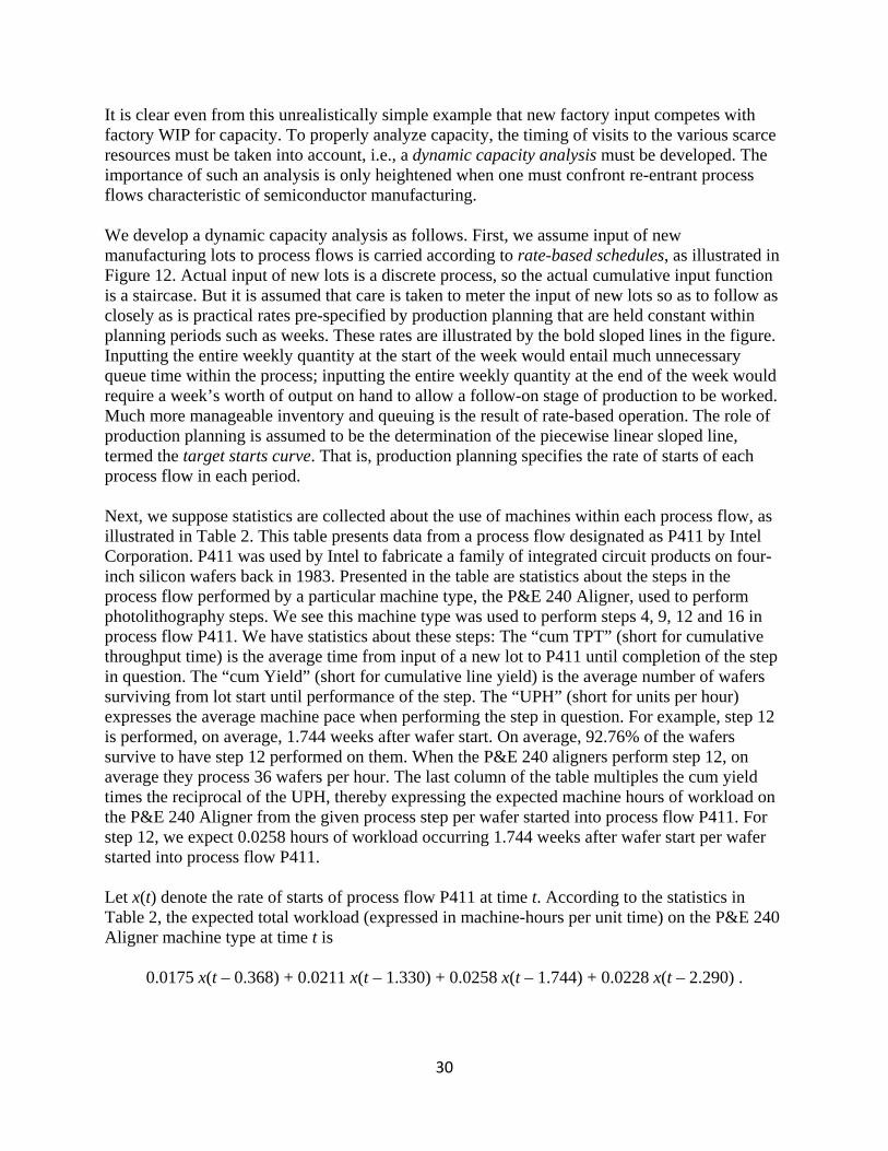
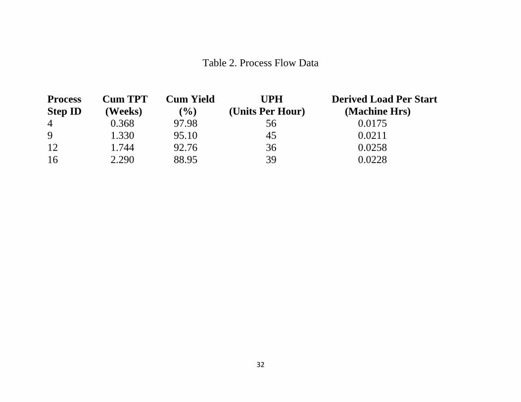
It is clear even from this unrealistically simple example that new factory input competes with factory WIP for capacity. To properly analyze capacity, the timing of visits to the various scarce resources must be taken into account, i.e., a dynamic capacity analysis must be developed. The importance of such an analysis is only heightened when one must confront re-entrant process flows characteristic of semiconductor manufacturing. We develop a dynamic capacity analysis as follows. First, we assume input of new manufacturing lots to process flows is carried according to rate-based schedules, as illustrated in Figure 12. Actual input of new lots is a discrete process, so the actual cumulative input function is a staircase. But it is assumed that care is taken to meter the input of new lots so as to follow as closely as is practical rates pre-specified by production planning that are held constant within planning periods such as weeks. These rates are illustrated by the bold sloped lines in the figure. Inputting the entire weekly quantity at the start of the week would entail much unnecessary queue time within the process; inputting the entire weekly quantity at the end of the week would require a week’s worth of output on hand to allow a follow-on stage of production to be worked. Much more manageable inventory and queuing is the result of rate-based operation. The role of production planning is assumed to be the determination of the piecewise linear sloped line, termed the target starts curve. That is, production planning specifies the rate of starts of each process flow in each period. Next, we suppose statistics are collected about the use of machines within each process flow, as illustrated in Table 2. This table presents data from a process flow designated as P411 by Intel Corporation. P411 was used by Intel to fabricate a family of integrated circuit products on four-inch silicon wafers back in 1983. Presented in the table are statistics about the steps in the process flow performed by a particular machine type, the P&E 240 Aligner, used to perform photolithography steps. We see this machine type was used to perform steps 4, 9, 12 and 16 in process flow P411. We have statistics about these steps: The “cum TPT” (short for cumulative throughput time) is the average time from input of a new lot to P411 until completion of the step in question. The “cum Yield” (short for cumulative line yield) is the average number of wafers surviving from lot start until performance of the step. The “UPH” (short for units per hour) expresses the average machine pace when performing the step in question. For example, step 12 is performed, on average, 1.744 weeks after wafer start. On average, 92.76% of the wafers survive to have step 12 performed on them. When the P&E 240 aligners perform step 12, on average they process 36 wafers per hour. The last column of the table multiples the cum yield times the reciprocal of the UPH, thereby expressing the expected machine hours of workload on the P&E 240 Aligner from the given process step per wafer started into process flow P411. For step 12, we expect 0.0258 hours of workload occurring 1.744 weeks after wafer start per wafer started into process flow P411. Let x(t) denote the rate of starts of process flow P411 at time t. According to the statistics in Table 2, the expected total workload (expressed in machine-hours per unit time) on the P&E 240 Aligner machine type at time t is
0.0175 x(t – 0.368) + 0.0211 x(t – 1.330) + 0.0258 x(t – 1.744) + 0.0228 x(t – 2.290) .
31
Figure 12. Rate-Based Scheduling of Process Flow Input
32
Table 2. Process Flow Data
Process Cum TPT Cum Yield UPH Derived Load Per Start Step ID (Weeks) (%) (Units Per Hour) (Machine Hrs) 4 0.368 97.98 56 0.0175 9 1.330 95.10 45 0.0211 12 1.744 92.76 36 0.0258 16 2.290 88.95 39 0.0228

33
Now let’s recall the assumption of rate-based production, whereby the start rate is held constant in pre-specified periods such as weeks. Let xt denote the rate of wafer starts into process P411 during week t, where week t is the time interval (t – 1, t ], t = 1, 2, …. , up to some planning horizon T. Let us consider the workload from a specific step experienced in a specific week under this assumption. Consider the workload from Step 12 experienced in week 3. For time measured in fractional weeks, week 3 begins at time 2.0 and ends at time 3.0. According to the statistics in Table 2, wafers undergoing Step 12 were input to the manufacturing process 1.744 weeks before the step is performed (on average). This means wafers input during the interval (2.0 – 1.744, 3.0 – 1.744] = (0.256, 1.256] experience Step 12 during week 3 (on average). Recalling our rate-based input assumption, the number of wafers started during (0.256, 1] is simply the fraction of week 1 represented by (0.256, 1] times the total wafers started in week 1, i.e., (1 – 0.256) * x1 = 0.744 x1. Similarly, the number of wafers started during (1, 1.256] is (1.256 – 1) * x2 = 0.256 x2. On average, each of these wafers contributes 0.0258 machine-hours of workload. That is, the workload on the P&E 240 Aligners in week 3 from performing Step 12 is
0.0258 ( 0.256 x2 + 0.744 x1 ).
Considering all steps in the P411 process flow, and generalizing this analysis to an arbitrary period t, the workload on the P&E 240 Aligners in week t from process flow P411 is expressed as
0.0175 ( 0.632 xt + 0.368 xt-1 ) + 0.0211 ( 0.670 xt-1 + 0.330 xt-2 ) + 0.0258 ( 0.256 xt-1 + 0.744 xt-2 ) + 0.0228 ( 0.710 xt-2 + 0.290 xt-3 )
Simplifying the expression, the workload on the P&E 240 Aligners in week t from process flow P411 is expressed as 0.01106 xt + 0.02718 xt-1 + 0.04235 xt-2 + 0.0066 xt-3 . (4)
Note that the workload in period t as expressed in (4) is a function of wafer starts (process flow input) in weeks t, t-1, t-2, and t-3. That is, to perform a proper capacity analysis one must specify the time history of process flow input. Next, we consider information about the capacity of the P&E 240 Aligner machine type. Uploading different factory data, we find that 7 of these machines are in service. The factory works 168 hours per week. Considering the committed cycle time (i.e., manufacturing lead time) for P411, the maximum utilization of the P&E 240 Aligner that management allows is 66%. For the purposes of planning production, the capacity of the P&E 240 Aligners is therefore
7 * 168 * 0.66 = 554.4 processing hours or workload per week.
We can now formulate a capacity constraint on production plan generation reflecting the capabilities and workloads on the P&E 240 Aligners:
34
0.01106 xt + 0.02718 xt-1 + 0.04235 xt-2 + 0.0066 xt-3 + {similar expressions for the workloads from other process flows utilizing the P&E 240 Aligners} 4.554 . (5) If the total workload in period t as calculated in the left hand side of (5) adds up to less than 554.4 machine hours, and similar constraints reflecting the limitations of the other process equipment and satisfied, then it is plausible that the starts proposed by the production plan can achieve target cycle times and meet target output schedules. But a workload higher than 554.4 would generate excessive queues for the P&E 240 Aligner, and achievement of target cycle times would be unlikely. In the latter case, good customer service would be difficult to achieve. Note that, for t 3, subscripts on certain production start variables are for periods before the first planning period, e.g., x0 denotes the starts made in the week before the first week of the plan, x-1 denotes the starts made two weeks before the first week of the plan, and so on. These are not variables; they are facts, and, as such, they are input data to the formulation of the capacitated loading analysis. In this way, capacity is reserved to complete the WIP flush, and new starts are allowed only as remaining capacity permits. The Planning Engine developed in research at the University of California at Berkeley carries out a generalized version of the foregoing analysis. The Engine admits planning periods of varying length (in turn reflecting the factory working calendars), time-varying yield, cycle time and UPH parameters, time-varying assignments of machine types to steps, alternative machine types at process steps, and time-varying equipment counts, factory working hours and maximum utilization parameters. At run time, the software generates the constraints suitable for a linear programming capacity analysis based on these data. Production plans generated by LP calculations subject to these constraints have been tested in detailed fabrication simulations simulating equipment down times and operational execution for industry data sets. The wafer start schedules proposed by the LP were fed into the simulations. Simulated cycle times and equipment utilizations agreed within 1% with those in the LP model, demonstrating the validity of the production plans (Hung and Leachman [1996]). Alternative Machine Types Non-homogeneous sets of machines that perform a basic kind of semiconductor fabrication step such as photolithography exposure are prevalent in semiconductor factories. To accurately represent capacity relationships in the planning model, one must expand the model. Depending on the nature of the alternatives, there are various formulation strategies that minimize the model complexity necessary to accurately model capacity. The simplest case is when process times are independent of the resource alternative selected, and the alternative machine types are nested. For example, suppose there are two types of exposure machines, type A and type B. Type B is a newer model that can perform any exposure step; type A is an older model that can perform only non-critical exposure steps. For this type of case, Leachman and Carmon [1992] show that ordinary capacity constraints defined for appropriate groups of machine types constitute an exact capacity model. For this particular example, two capacity constraints per period constitute an exact model. One constraint limits the total workload of critical steps by the available processing time of machine type B, and the other

35
limits the total workload of all exposure steps to the sum of available processing times of both machine types. This approach also provides an exact model when process times of the nested machine types are proportional, since available processing times of alternative machine types may be appropriately scaled according to the process times of one machine type chosen as a standard. A more difficult case arises when machine usage patterns are not nested. For example, suppose now there are three exposure machine types. Suppose some process steps must be performed on either machine types A or B, other process steps must be performed on either machines types B or C, and still others must be performed on machine types A or C. These more general patterns of allowed allocation of machines arise when engineering effort is expended to qualify machines one by one for critical process steps, and certain machines are found to perform better than others. The restrictions placed on machine allocation are thus an avenue for securing better process control and higher yields, albeit at the potential expense of reduced capacity and longer manufacturing lead times. When alternative machine types exhibit this more general pattern of allowed assignments to process steps, Leachman and Carmon [1992] show that the most compact exact model requires introduction into the model of new variables that allocate step workloads to the resource types. The most difficult case of machine arrangement involves dynamic machine arrangement constraints, whereby the set of qualified process machines at one step is dependent on the machine type assigned at some previous process step. Efforts to achieve process control on the most advanced digital process technologies in the industry sometimes include dynamic machine allocation constraints between critical photolithography exposure steps, or between the lithography exposure step and the following etching step. (In such cases, most of the machine “types” are individual machines.) To illustrate dynamic arrangement constraints, suppose the qualified machines for the first critical exposure step are machines A, B and C. If machine A is selected, then the qualified machines for the second critical exposure step are machines A or C. If machine B is selected at the first step, then the qualified machines for the second critical exposure step are machines B or D. Thus the qualified machines for performing the second critical step vary according to which machine was utilized at the first critical step. To properly model capacity constraints in this case, the allocation of workloads to machines at different steps must be constrained so as to be consistent, if planned lead times are to be observed. Lin [1999] shows that this case is most efficiently modeled using routing variables that schedule the release of WIP for movement through particular machine types at downstream critical steps. Mitigating Horizon Effects Without special care taken, the optimal solution of a formulation of the capacitated loading problem incorporating constraints as above will exhibit peculiar, undesirable behavior near the horizon T of the model. Variables for production starts in periods within one lead time of the horizon will be set equal to zero, since they do not contribute to demands included in the formulation. Variables for the release rates in periods just before this will typically have surprisingly large values. Such unreasonably large values are feasible since they do not have to

36
compete for capacity with starts in subsequent periods. The tacit assumption that production is permanently terminated at the horizon T is the root cause of this undesirable behavior. To overcome this problem, one can incorporate into the formulation a steady-state horizon condition (Leachman [1993]). Let Li denote the production lead time for product i. The interval [T-Li, T] is termed the frozen interval for product i. Production starts of product i in all time periods that intersect the frozen interval are constrained to be equal, i.e., a single variable is utilized to represent starts in each of these periods (multiplied by an appropriate scaling constant if there are differences in period lengths). For the purposes of enforcing inventory balance of product i and resource consumption in capacity constraints, an additional time period is appended on to the planning horizon, with length equal to Li working days., Demand for product i in this period is set to be the same rate as the average rate in the frozen period. Inventory and backorders of completed product i are measured in the objective function at both the start and the end of the extra period. Optimal solutions to formulations including this steady-state condition provide productions plans that exhibit smooth production near the horizon. Incorporating Marketing Strategies and Policies into the Calculation of Production Plans There are two critical areas of marketing strategy and policy with respect to production plan generation. First, typically it is infeasible to fulfill all demands on time. Market potential for “hot” new products may be very high. There may be insufficient finished goods inventory, insufficient work-in-process or insufficient yields and capacities. Guidance is required to determine which demands to delay or defer. Second, production scheduled in response to forecasted demands not yet materialized in the form of customer orders represents a risk. If such demands do not materialize, there is wasted investment in materials, and wasted deployment of machine and labor resources that could have been deployed in production of other products that could be sold. If the demands materialize but materialize later than forecast, there is the risk that the selling price may have declined by that time. The investment in materials and the allocation of labor of resources might have been more profitably utilized to make other products sold at higher prices. Guidance is required as to how much production risk to take for the various types of products. The following structural approach is proposed to deal with the first area of concern. Priority classes are defined for demands of all products. On-time delivery of class 1 demands is paramount. Subject to the best-achievable performance for class 1 demands, class 2 demands are made as on-time as possible, and so on. There is no economic trade-off allowed between demands belonging to different classes; on-time performance in class n is taken as a constraint on planning on-time performance of class n+1. In principle, there can be any number of demand classes. The demand classes are organized into three types of classes. The highest-priority classes are order classes; these classes include all prior commitments to customers. Multiple classes of this type are desirable if things are so bad that many prior commitments cannot be honored, and
37
considerable orders will be delayed from promise dates. In such a case, there is a stratification of orders based on the seriousness of customer impacts. For example, orders for customers whose own production lines are shut down awaiting parts could be placed in Class 1, whereas orders for customers whose inventories are not yet exhausted could be placed in Class 2. After the order classes, the next lower priority classes are members of a class type termed safety stock rebuild classes. Because of uncertainties in the supply chain, e.g., uncertain yields, uncertain lead times, uncertain machine capacity, etc., safety stocks made be required to ensure on-time delivery. If the levels of such inventories are below targets, they should be replenished before additional customer commitments are made, if good on-time delivery performance is to be achieved. Additionally, the marketing department may have made a commitment to service new demands for certain products from a finished goods inventory or a semi-finished goods inventory rather than forcing customers to wait out the lead time for new production. This commitment implies certain inventory levels; if inventories are below these levels, they need to be replenished in order to offer the targeted customer service. The last type of demand class, termed forecast classes, includes all forecasted demands not accounted for by the order and inventory rebuild classes. Even within this type multiple demand classes may be useful as a means of managing the risks of forecast errors. For example, suppose forecast errors for each product are tracked. Imagine taking the total forecast demand for a product, less demand for the product included within the order and stock rebuild classes, and less one standard deviation of forecast error. This represents the portion of forecasted demand that has a relatively high probability of being realized. The remaining one standard deviation of the forecast error is put in the next class of demand. This represents the risky portion of forecasted demand. By placing it in a lower-priority class, production resources will be allocated to low-risk demands first and high-risk demands second. Within the same class, there needs to be some prioritization of demands for different products. It is proposed to achieve this by pursuing a discounted cash flow objective function within each class. Within order classes and safety stock rebuild classes, all cash flows are negative, and we seek to minimize the costs of fulfilling customer orders or rebuilding safety stocks. Costs that are included in the objective are shortage costs for each product and avoidable costs of new production starts. Shortage costs are taken to be proportional to the average selling prices for products. As a result, shortages of high-revenue products are cleared first. Within forecast classes, cash flows are both positive and negative. Positive cash flows in the objective are the revenues for product sales (awarded at time of output or time of demand, whichever is later), estimated as the average selling price times quantity supplied. Negative cash flows are the avoidable costs of production starts. A production plan is prepared maximizing discounted cash flow to the company, subject to best-possible on-time delivery performance in higher-priority demand classes. Because all revenues and costs are discounted, demand opportunities are filled as soon as is feasible. Moreover, there is no excess production nor is there any excessively early production. Let R denote the total number of demand classes. A series of linear programming calculations is to be made, solving one linear program per demand class. Let LPr denote the linear program to be solved for class r, r = 1, 2, …, R. One might think an extraordinary amount of computation would be involved to perform optimization calculations for each class when demand is stratified into many classes. But such is not the case. To see why, for a given product, let r
tD denote the
38
cumulative demand for the product at time t, cumulative over time and cumulative over demand classes 1, 2, …, r, r = 1, 2, …., R. The linear program formulated for class r is solved for demand inputs r
tD . Let rtX denote the cumulative output of the product planned in LPr. r
tX is not a
variable of the linear program, but it is an affine function of the variables of LPr. Let rtI denote
the finished goods inventory of the product at time t as planned in LPr, and let rtBO denote the
amount of shortage of the product at time t, as planned in LPr. (“BO” is short for backorders, another name for delayed demands.) The constraint for mass conservation at time t in LPr for the product in question takes the form:
rt
rt
rt
rt DBOIX .
Formulated this way, note that zero production is a feasible solution to LPr, i.e., LPr is always feasible (i.e., one can simply backorder all demands), and therefore it always has an optimal solution. Let 1r
tBO denote the optimal value of the shortage at time t of the product, as calculated
in LPr-1. In the formulation of LPr, we include upper bounds on shortage variables as follows:
11 rt
rt
rt
rt DDBOBO .
Comparing LPr-1 and LPr, these formulations have the same variables and the same structural constraint sets. The only differences are in the right hand side values of demand constraints ( r
tD
in lieu of 1rtD ) and in the bounds on backorder variables. With minor modification, the optimal
solution to LPr-1 provides a feasible starting solution for LPr: one simply increments the values of the shortage variables 1r
tBO to be 11 rt
rt
rt
rt DDBOBO and changes the right-hand side
values from 1rtD to r
tD . If switching from a safety stock rebuild class to a forecast class, the
objective function must be changed, but again, a feasible starting solution is at hand. Figure 13 illustrates this strategy. Depicted are 1r
tD , rtD , and 1r
tX (the optimal supply of the
product calculated by LPr-1). In this example, up until time t0 demands 1rtD and r
tD are
coincident, but after that time additional demands are presented by rtD . The production plan
1rtX starts out running ahead of 1r
tD but demands soon outstrip capacity, resulting in shortages.
It is the best that can be done. At an arbitrary time t, the cumulative output plan rtX must not lie
below 1rtX , i.e., the planned shortage is bounded above by the previously calculated shortage
1rtBO plus the increment in demands 1r
tD - rtD . This corresponds to backordering all the new
demands plus the backorders found necessary to the higher-priority demands. Any greater amount of backordering corresponds to diminishing the customer service calculated for previous classes.
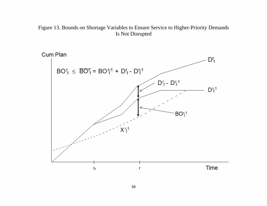
39
Figure 13. Bounds on Shortage Variables to Ensure Service to Higher-Priority Demands Is Not Disrupted
t0 t
40
In actual industrial large-scale calculations, the time required to optimize five demand classes took about twice the time to optimize the first demand class. Thus considerable richness in marketing strategy can be accommodated without enlarging the linear programming matrix from that required for a single demand class. It is simply a matter of solving for multiple objective functions and adjusting the values for the right hand side and the variable upper bounds. It is proposed to address the second area of marketing concern as follows. Each product in the product structure is declared by Marketing to be either build-to-plan (BTP) or build-to-order (BTO). Consistency within the product structure is required in the sense that BTO products may not be inputs to BTP products. A target inventory for BTP products may be declared at its corporate inventory point; replenishment of same is included in one of the safety stock demand classes. Within the linear programming formulations for forecast demand classes, the period one production start variable for each BTO product is bounded above by the optimal value of the corresponding variable in the linear program for the last safety stock rebuild demand class. Production start variables in subsequent variables are not so bounded. This technique ensures production in the first period is solely for customer orders or inventory replenishments. Production planned for subsequent periods includes response to forecasts. If the production plan is regenerated every period, then production of BTO products is only ever undertaken to meet customer orders or to replenish safety stocks. However, because planned production in periods 2 and thereafter considered forecast demands, availability of the products was generated. As orders consuming the availability materialize, production will be scheduled (assuming the production plan is regenerated). Again, responding to this concern does not require any structural change to the LP matrix, i.e., no additional rows or columns are required. It is simply a matter of incorporating the appropriate upper bounds on period one production variables for the BTO products in formulations for forecast classes. Objective Functions In the author’s experience, when attempting to develop a production planning system based on mathematical programming, the most controversial aspect of the methodology concerns the objective function or objective functions to be utilized. There is typically little controversy over the constraints. Everyone agrees that production plans must be feasible; the plans should reflect mass conservation of available machine and labor services and of products and raw materials, and appropriate lead times should be allowed for process flows considering the queues involved. But different departments in a corporation have different scopes and different objectives, sometimes conflicting. Marketing is concerned with on-time delivery and capturing the market revenue potential. Manufacturing is concerned with managing bottlenecks and maintaining stable workloads. Central Planning is concerned with wise allocation of products among alternative plants. This means allocating demands to expensive subcontractors only when in-house capacity is saturated. It also means that, when there are alternative plants to make the same product, consideration should be given to the relative yields and relative manufacturing lead times for the
41
alternative sources. Finally, Finance will be concerned with profit and loss implications of the plan. The strategy proposed herein rests on a foundation of the following principles: (1) On-time delivery performance to prior customer commitments takes precedence over cash flow from new sales. Bumping customer deliveries of lower-margin products in order to sell increased amounts of higher-margin products is viewed as a false economy. Typically, large industrial customers do not buy one product; they buy many products, both low-margin ones and high-margin ones. A shortage of a low-margin product can be just as damaging to the customer as a shortage of a high-margin product; it can shut down the customer’s production line just as a shortage of a high-margin product could shut it down. Poor customer service on low-margin products is likely to dissuade the customer from buying any product. (2) On-time delivery performance for replenishment of safety stocks is lower priority than honoring prior customer commitments, but takes precedence over generating availability for future sales. Risk of delivery failures must be controlled before generating additional commitments. As discussed above, within each demand class, we propose to maximize discounted cash flow. This approach rests on the following principles. (3) When it is impossible to provide on-time delivery of customer commitments for both products A and B then priority is given to the product with the higher average selling price. (4) When it is impossible to provide on-time delivery of safety stock replenishments for both products A and B then priority is given to the product with the higher average selling price. (5) When it is impossible to meet the portions of demand forecasts in excess of customer commitments and safety stock replenishments for products A and B, priority is given to demands for the product with maximum margin, i.e., average selling price less avoidable production cost. (6) The primary variables of the production plan are new production starts, and the sourcing of those starts at corporate inventory points. Work-in-process resident in between corporate inventory points is not re-scheduled; that is, the out schedule for WIP at the next corporate inventory point is an input to the planning decision, not an output of it. (7) Capacity required for the WIP flush up to the next corporate inventory point takes precedence over capacity consumption by new production. We maintain that the proposed objective functions and demand class structure satisfy, to the maximum extent feasible, the concerns of Marketing, Manufacturing, Central planning and Finance. The satisfaction of Marketing concerns already has been discussed. As for Manufacturing, the choice of variables in the formulation ensures that WIP is never re-scheduled. All schedules for production starts are rate-based, changing rate only at the period boundaries. Capacities of resources as defined by manufacturing are observed, i.e., bottlenecks
42
are never overloaded (unless already overloaded by initial WIP). If the market forecasts are sufficient, bottlenecks will be loaded to capacity as the formulation pursues maximum cash flow. As for Central Planning, avoidable costs for subcontracted production are much higher than for in-house production; thus subcontracting is utilized only when in-house capacity is inadequate. Moreover, when there are alternative routes with differing yields or lead times, the minimization of the discounted avoidable production costs means routes with higher yields are preferred (less production is required) and routes with shorter lead times are preferred (production may be started later, thereby reducing discounted costs). Finally, Finance can be assured that the plan presents the maximum possible discounted cash flow for the corporation, subject to fulfillment of customer service commitments, appropriate mitigation of supply risks, and subject to manufacturing capabilities. Demand is “pulled” through the factories in the sense that production is not started early unless necessary for reasons of capacity smoothing. (It is not started earlier than necessary because the production costs are discounted, and so starting later reduces costs.) Moreover, because cumulative demand constraints are formulated, demand opportunities never go away, and market potential as captured as soon as manufacturing capabilities permit. One interesting strategy for deploying the demand class structure is to define two order classes as follows. Class 1 includes customer commitments, sorted by the delivery date promised to the customer. Class 2 includes the same customer commitments, but now sorted by the customer’s request date. The customer request date is always earlier than or equal to the promise date. Although the total demand for each product is the same in these two classes, demand may occur earlier in the second class, and hence the cumulative curve for class 2 sometimes lies above the cumulative curve for class 1. In that sense, class 2 has “more” demand than does class 1. Solving the LPs for such classes produces a desirable business result: On-time delivery to customer promise dates is made is on-time as possible; given that performance, if it is possible to move up delivery of some order towards the customer request date without bumping service to promise dates for other products, then that is scheduled into the plan. In this way, the plan not only strives to achieve optimal on-time delivery to customer commitments, it also strives to optimize progress on improving deliveries towards the original customer request dates. Persistence in Planning An issue that arises in the repeated generation of production plans updated on a rolling horizon basis concerns what portions, if any, of the previous production plan should be frozen and exempt from revision, i.e., how much persistence of a previous plan in the new plan should there be. An approach to this issue suggested by some software vendors and some authors is to establish a time fence whereby plans within some short horizon are fixed and not changed in the new plan. In the author’s opinion, this is a meat-axe approach to the problem. A more thoughtful approach would consider, on the basis of sound business management, what decisions ought to persist vs. those that should be revisable in light of new information. It is asserted that the following things ought to persist: - On-time delivery to customer commitments, to the maximum extent feasible.
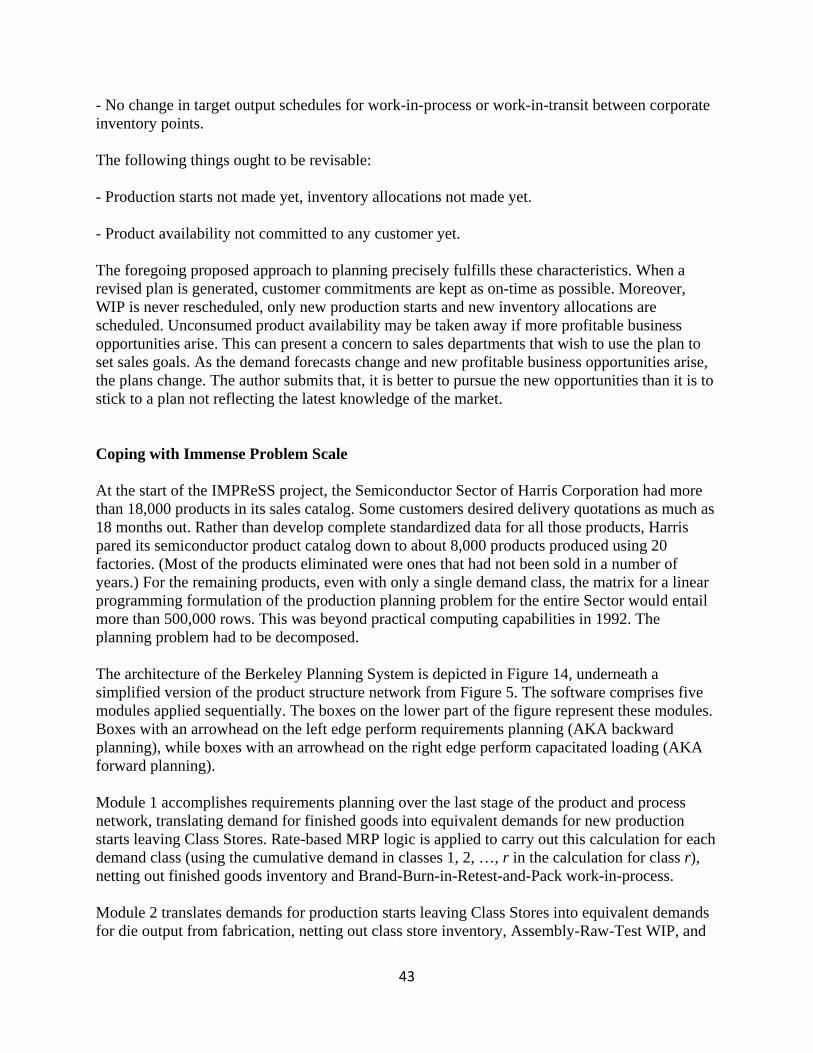
43
- No change in target output schedules for work-in-process or work-in-transit between corporate inventory points. The following things ought to be revisable: - Production starts not made yet, inventory allocations not made yet. - Product availability not committed to any customer yet. The foregoing proposed approach to planning precisely fulfills these characteristics. When a revised plan is generated, customer commitments are kept as on-time as possible. Moreover, WIP is never rescheduled, only new production starts and new inventory allocations are scheduled. Unconsumed product availability may be taken away if more profitable business opportunities arise. This can present a concern to sales departments that wish to use the plan to set sales goals. As the demand forecasts change and new profitable business opportunities arise, the plans change. The author submits that, it is better to pursue the new opportunities than it is to stick to a plan not reflecting the latest knowledge of the market. Coping with Immense Problem Scale At the start of the IMPReSS project, the Semiconductor Sector of Harris Corporation had more than 18,000 products in its sales catalog. Some customers desired delivery quotations as much as 18 months out. Rather than develop complete standardized data for all those products, Harris pared its semiconductor product catalog down to about 8,000 products produced using 20 factories. (Most of the products eliminated were ones that had not been sold in a number of years.) For the remaining products, even with only a single demand class, the matrix for a linear programming formulation of the production planning problem for the entire Sector would entail more than 500,000 rows. This was beyond practical computing capabilities in 1992. The planning problem had to be decomposed. The architecture of the Berkeley Planning System is depicted in Figure 14, underneath a simplified version of the product structure network from Figure 5. The software comprises five modules applied sequentially. The boxes on the lower part of the figure represent these modules. Boxes with an arrowhead on the left edge perform requirements planning (AKA backward planning), while boxes with an arrowhead on the right edge perform capacitated loading (AKA forward planning). Module 1 accomplishes requirements planning over the last stage of the product and process network, translating demand for finished goods into equivalent demands for new production starts leaving Class Stores. Rate-based MRP logic is applied to carry out this calculation for each demand class (using the cumulative demand in classes 1, 2, …, r in the calculation for class r), netting out finished goods inventory and Brand-Burn-in-Retest-and-Pack work-in-process. Module 2 translates demands for production starts leaving Class Stores into equivalent demands for die output from fabrication, netting out class store inventory, Assembly-Raw-Test WIP, and
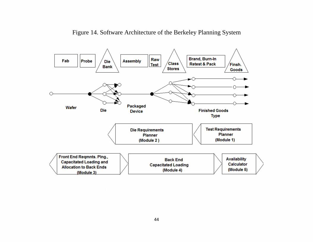
44
Figure 14. Software Architecture of the Berkeley Planning System

45
Die Bank inventory. Linear programs are formulated and solved as required to correctly plan die output requirements in the face of the substitution network at Die Bank and the binning and substitution networks in Raw Test and at Class Stores. Again, calculations are made for each demand class using demands cumulative over the higher-priority classes. As a computational strategy, the formulations for each demand class of a product family are collected into a single formulation, and formulations for up to 20 product families are collected into a single formulation. From experience, it was found that collecting these small linear programs into a larger linear program saved some computational time. In addition to the linear programming calculations, Revenue per assembly start item is calculated as a translation of the weighted average of the average selling prices for finished goods using that assembly item (taking account of yield losses and planned allocation of class stores items). Module 3 performs capacitated loading of fabrication and probe facilities. WIP-out projections of WIP past Wafer Bank are included in the formulation to determine a schedule for new production starts into fab and new starts leaving Wafer Bank. Revenue per die used in the objective functions is calculated based on a weighted average of the revenues per assembly start item calculated by Module 2. Module 4 performs capacitated loading of Assembly and Test facilities, taking the die supply calculated by Module 3 as a constraint while striving to meet the prioritized demands for finished goods. Finally, Module 4 takes planned worldwide output of finished goods and subtracts customer commits to determine product availability for use in delivery-date quotation. Splitting capacitated loading into sequential optimization calculations like this is, in general, suboptimal. It is conceivable that a severe bottleneck in assembly-test could block processing of die planned by Module 3. But this risk is low for the following reasons: (1) Fabricated dice can be placed in multiple types of packages and given many testing, burn-in and packing options. Assembly and test capacity constraints are for the most part separated by package type and testing option type. Despite tight capacity for one package type or testing option type, the die can still be sold under other options. (2) The capital investment in fabrication and probe facilities is more than an order of magnitude greater than that for assembly and test facilities. It is management’s strong desire that productivity of the fabrication asset should never be held back by assembly-test limitations. When planning capital investments, care is taken to make sure fab output is never held back by assembly-test capacity. While capacity constraints in fabrication are expensive and time-consuming to ease, constraints in assembly-test are relative cheaper and quicker to ease. Even for this serial decomposition of the planning problem, company-wide Module 3 and Module 4 calculations would have been too large for 1992 computing capabilities. Parallel decomposition also was engineered, as depicted in Figure 15. A single instance of Module 1, employing rate-based MRP computations, was deployed against worldwide data. Results for the six product lines were allocated to three UNIX workstation computers each running the Module 2 software. Requirements planning of die were conducted in parallel for the products belonging to pairs of product lines. These die requirements were allocated to two different instances of the Module 3 software, one handling the capacitated loading of the fabrication and probe facilities in
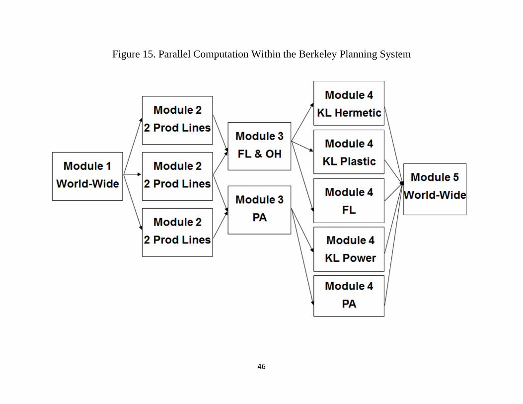
46
Figure 15. Parallel Computation Within the Berkeley Planning System

47
Pennsylvania that fabricated power products, the other handling the capacitated loading of all products at the fabrication and probe facilities in Florida and Ohio. These different product sets did not share capacity, so there was no loss of optimality by making separate, parallel capacity analyses of them using two parallel UNIX work station computers. The resulting die supply was allocated among five UNIX work stations, each equipped with the Module 4 software and each performing capacitated loading on a distinct set of assembly-test resources. These sets included hermetic package assembly and test in Kuala Lumpur, Malaysia; plastic package assembly and test in Kuala Lumpur, Malaysia; power product assembly and test in Kuala Lumpur, Malaysia; assembly-test in the Florida site; and assembly-test in the Pennsylvania site. Finally, a single Module 5 calculation was performed to determine availability of all products. The largest of the Module 3 instances solved linear programs with 60,000 – 70,000 constraints. The largest of the Module 4 instances solved linear programs with nearly 130,000 constraints. It was found that the interior point method was able to solve the Module 4 linear programs with more than 100,000 rows faster than could the simplex algorithm, but for the smaller linear programs in Module 2 and Module 3, the simplex algorithm was faster. A regenerative planning cycle was carried out every weekend at Harris. Considering the time window from start-of-Saturday midnight to start-of-Monday midnight at all manufacturing sites worldwide, only 17 hours was available to complete a planning cycle in time to make production start schedules available for the first shift on Monday. The total planning cycle for a full regenerative plan was 15-16 hours when the IMPReSS system began official use in the second half of 1992; within a year, the planning cycle time had been reduced to about 12 hours, with continued refinement in subsequent years. At the time of implementation, both IBM and Cplex reported that Harris was solving the largest linear programs on a frequent basis of any of their customers. The same five UNIX work stations crunching out a production plan on the weekend were used for maintenance of data in the databases supporting planning during the work week. This made for low computer hardware and software requirements for the planning system. IMPReSS History Up until 1988, the Semiconductor Sector of Harris Corporation was focused on the design and fabrication of integrated circuits for aerospace and military applications. Harris possessed strong patents on a specialized fabrication process generating so-called “rad-hard” (radiation-hardened) integrated circuits. Ordinary semiconductors are not resistant to solar radiation once taken out of the earth’s atmosphere. But chips fabricated using the Harris’ rad-hard process were insensitive to solar radiation. Thus Harris dominated the military and aerospace markets for integrated circuits. Harris would license integrated circuits designed by other companies to fabricate and market “rad-hard” versions of those products. This niche marketing strategy worked well for many years. The Semiconductor Sector had a profitable business, and rapid technological progress was fueled by substantial military funding and demand for advanced circuitry. But, by the late 1980s, the strategy was faltering. Space exploration expenditures had declined sharply compared to the 1960s and 1970s. The Cold War with the Soviet Union also was winding down, reducing expenditures on missiles and rocketry.

48
At the same time, the economic scale of fabrication facilities able to process leading-edge digital circuits continued to grow. Harris found itself in the situation whereby their dominant market share of the military-aerospace market provided insufficient volume to fill an economic-scale leading edge fabrication facility. Meanwhile, under the leadership of CEO Jack Welch, General Electric put its entire semiconductor business up for sale. This included the former Intersil products and factories, the former RCA Solid State products and factories, and GE proper products and factories. These three businesses had not been truly merged by GE. They had separate sites, separate managements, and separate business systems. Because the while business was up for sale, little or no effort was put into rationalizing it. Harris made the bold decision to buy GE’s entire semiconductor business, including all products, factories and employees. The deal closed on December 31, 1988. In so doing, the Semiconductor Sector was tripled in size, and took on much debt. The acquisition changed the Semiconductor Sector in profound ways. Beforehand, almost all semiconductor production was tied to programmed government acquisitions of military or aerospace equipment. Marketing was mainly a process of designing components of use to the government for its programs and preparing successful proposals. Manufacturing management was to a great extent program management, insuring contracts for the requisitioned components were faithfully met. For most products, Harris had no real competition. Afterwards, Harris was plunged into competitive markets for which there were many alternative suppliers. Customers of GE products operated their own production lines to assemble automobiles, robotics or switching equipment used in telecommunication networks. They expected quotations of delivery dates at time of order, and they expected those dates to be honored. Harris had little experience with such types of customers. Pressure was on Semiconductor Sector management to realize savings from the merger. Like process technologies from the predecessor companies were grouped into single manufacturing sites. Fabrication process technologies for analog products were concentrated in the former RCA fabrication lines in Findlay, Ohio; process technologies for power products were concentrated in the former GE fabrication lines in Mountaintop, Pennsylvania; and process technologies for digital technologies and “rad-hard” process variants were concentrated in the former Harris fabs in Palm Bay, Florida. There was a similar rationalization of assembly-test factory roles. With production of former Intersil, RCA, GE and Harris products shifting into manufacturing facilities of different predecessor companies, the four separate legacy business systems became a big problem. Production planners and customer service agents lost visibility to work-in-process, inventory and factory production decision-making. On-time delivery performance became poor, averaging about 75% in 1989, likely the worst performance among all major semiconductor

49
merchants at the time. By the end of the year, there were more than 5,000 delinquent line-items, an incredible number.2 Compared to the combined 1988 semiconductor sales of GE and Harris, Harris semiconductor sales dropped by more than $100 million in 1989. Large customers for former GE products informed Harris they intended to eliminate Harris as a vendor as soon as they could. It was painfully clear to Harris management that the on-time delivery weaknesses had to be rectified or the Sector would be plunged into bankruptcy. Harris management reviewed how other semiconductor firms addressed on-time delivery. They concluded it was unwise to simply emulate what much larger companies such as Texas Instruments, Motorola, NEC or Intel did; those companies could always outspend Harris. Instead, Harris management decided it would try to outsmart them. Starting in 1987, Harris sponsored the development of advanced production planning systems for semiconductor manufacturing at the University of California at Berkeley, under the direction of Professor Robert C. Leachman. The results of this research became known in the industry as the Berkeley Planning System (BPS). During the period 1987-1989, Harris applied BPS on a relatively small scale, addressing the planning of production of three fabrication facilities in Palm Bay, Florida. Interfaces to factory floor databases were developed, and automated planning of the fabs was achieved. Harris’ fab planners were pleased with the system; it saved them manual work, it analyzed more information than they could beforehand, and plans could be routinely updated at any time. This success encouraged Harris to develop a company-wide automated production planning and delivery quotation system spanning all semiconductor products in all factories. The new system to be developed and implemented at Harris was given the name IMPReSS – short for Integrated Manufacturing Production Requirements Scheduling System (Leachman et al [1996]). The IMPReSS project was launched in June, 1990. Professor Leachman took a one-year leave of absence from U. C. Berkeley to direct the IMPReSS project full-time at Harris. The IMPReSS project spanned the following areas of effort:
- Developing and implementing standardized databases across all factories and at the Palm Bay headquarters supporting automated production planning and delivery quotation
- Development of product structure (AKA bill of materials) and capacity data, and databases for same
- Installation of a demand forecasting system - Enhancement of the delivery quotation system - Development and enhancement of BPS for robust company-wide application
The last task was primarily carried out by Professor Leachman’s PhD students remaining in residence at U. C. Berkeley. A number of Berkeley bachelors and masters students worked as summer interns at various Harris sites in performance of the first two tasks.
2 A line‐item is a scheduled delivery of one product on one date. A typical customer order included multiple line items (because multiple deliveries were requested and/or deliveries of multiple products were requested. The on‐time delivery metric measures the percentage of line‐items delivered when promised.

50
Executive leadership of the IMPReSS project was impressive. Jon Cornell, CEO of the Semiconductor Sector, had built has own linear programming model for fab production planning when he was a fab manager. He recognized the potential of advanced operations research. An IMPReSS insignia was designed and printed on polo shirts issued to all project staff. Wearing an IMPReSS shirt himself, Cornell called a company-wide kick-off meeting and addressed the entire organization. (Remote sites attended via closed-circuit television.) Cornell asserted that the IMPReSS project was the most important project in the company. If the on-time delivery problem was not solved, the company had no future. Everyone must do whatever was needed to ensure the project was successful. In retrospect, the most difficult task was converting the entire company to a standard data model reflecting the standard product and process structure depicted in Figure 5. The databases in the various factories of the legacy companies defined differing boundary points between process flows and products and different product structures. These structures reflected differences in management organization, differences in the data structures allowed in factory floor systems, and differences in management philosophy. Examples:
- Many sites had inventory points between fab and probe and between assembly and test, prompted by the fact that the serial facilities had separate managements desiring asynchronous production schedules.
- The process flows defined in manufacturing execution systems for fabrication areas were
usually fab-in to fab-out flows, even though product names typically changed at wafer bank. Each product was assigned to such a flow, even though the product actually existed only on one side of wafer bank or the other. For example, if base wafer A served as the source material for wafer types A1 and A2, the factory floor database would show products A, A1, A2 were all products processed from fab-in to fab-out. Production control staff would manually re-label the product for a given manufacturing lot of product A once disposition of the lot between A1 and A2 was decided. Without data on the product structure, this business process was not automatable.
- Harris proper tended to have much fewer usable bins of quality and fewer finished goods
than the more commercial GE, RCA and Intersil products. The Harris proper managers preferred a product structure where one product name was used all the way through the test facility, with no inventory held at class stores. While perhaps suitable for the military aerospace business, it was an ill-suited strategy for the commercial products.
For many Harris staff not working on the factory floor and/or not intimate with the technical details of process and product design, the data presented in company databases was reality to them. It was quite discomforting to find out that the real product structure was actually quite different from what was presented in computer databases. The conversion upset long-held intuitions and conventions. But simply taking the union of all extant data structures was not a feasible option. This would have resulted in too many corporate inventory points for computationally-feasible linear programming calculations. Moreover, many changes were
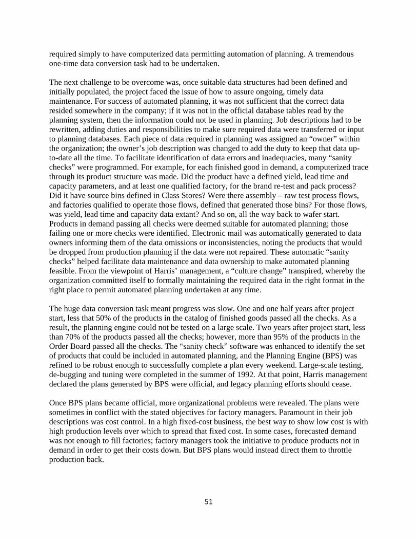
51
required simply to have computerized data permitting automation of planning. A tremendous one-time data conversion task had to be undertaken. The next challenge to be overcome was, once suitable data structures had been defined and initially populated, the project faced the issue of how to assure ongoing, timely data maintenance. For success of automated planning, it was not sufficient that the correct data resided somewhere in the company; if it was not in the official database tables read by the planning system, then the information could not be used in planning. Job descriptions had to be rewritten, adding duties and responsibilities to make sure required data were transferred or input to planning databases. Each piece of data required in planning was assigned an “owner” within the organization; the owner’s job description was changed to add the duty to keep that data up-to-date all the time. To facilitate identification of data errors and inadequacies, many “sanity checks” were programmed. For example, for each finished good in demand, a computerized trace through its product structure was made. Did the product have a defined yield, lead time and capacity parameters, and at least one qualified factory, for the brand re-test and pack process? Did it have source bins defined in Class Stores? Were there assembly – raw test process flows, and factories qualified to operate those flows, defined that generated those bins? For those flows, was yield, lead time and capacity data extant? And so on, all the way back to wafer start. Products in demand passing all checks were deemed suitable for automated planning; those failing one or more checks were identified. Electronic mail was automatically generated to data owners informing them of the data omissions or inconsistencies, noting the products that would be dropped from production planning if the data were not repaired. These automatic “sanity checks” helped facilitate data maintenance and data ownership to make automated planning feasible. From the viewpoint of Harris’ management, a “culture change” transpired, whereby the organization committed itself to formally maintaining the required data in the right format in the right place to permit automated planning undertaken at any time. The huge data conversion task meant progress was slow. One and one half years after project start, less that 50% of the products in the catalog of finished goods passed all the checks. As a result, the planning engine could not be tested on a large scale. Two years after project start, less than 70% of the products passed all the checks; however, more than 95% of the products in the Order Board passed all the checks. The “sanity check” software was enhanced to identify the set of products that could be included in automated planning, and the Planning Engine (BPS) was refined to be robust enough to successfully complete a plan every weekend. Large-scale testing, de-bugging and tuning were completed in the summer of 1992. At that point, Harris management declared the plans generated by BPS were official, and legacy planning efforts should cease. Once BPS plans became official, more organizational problems were revealed. The plans were sometimes in conflict with the stated objectives for factory managers. Paramount in their job descriptions was cost control. In a high fixed-cost business, the best way to show low cost is with high production levels over which to spread that fixed cost. In some cases, forecasted demand was not enough to fill factories; factory managers took the initiative to produce products not in demand in order to get their costs down. But BPS plans would instead direct them to throttle production back.
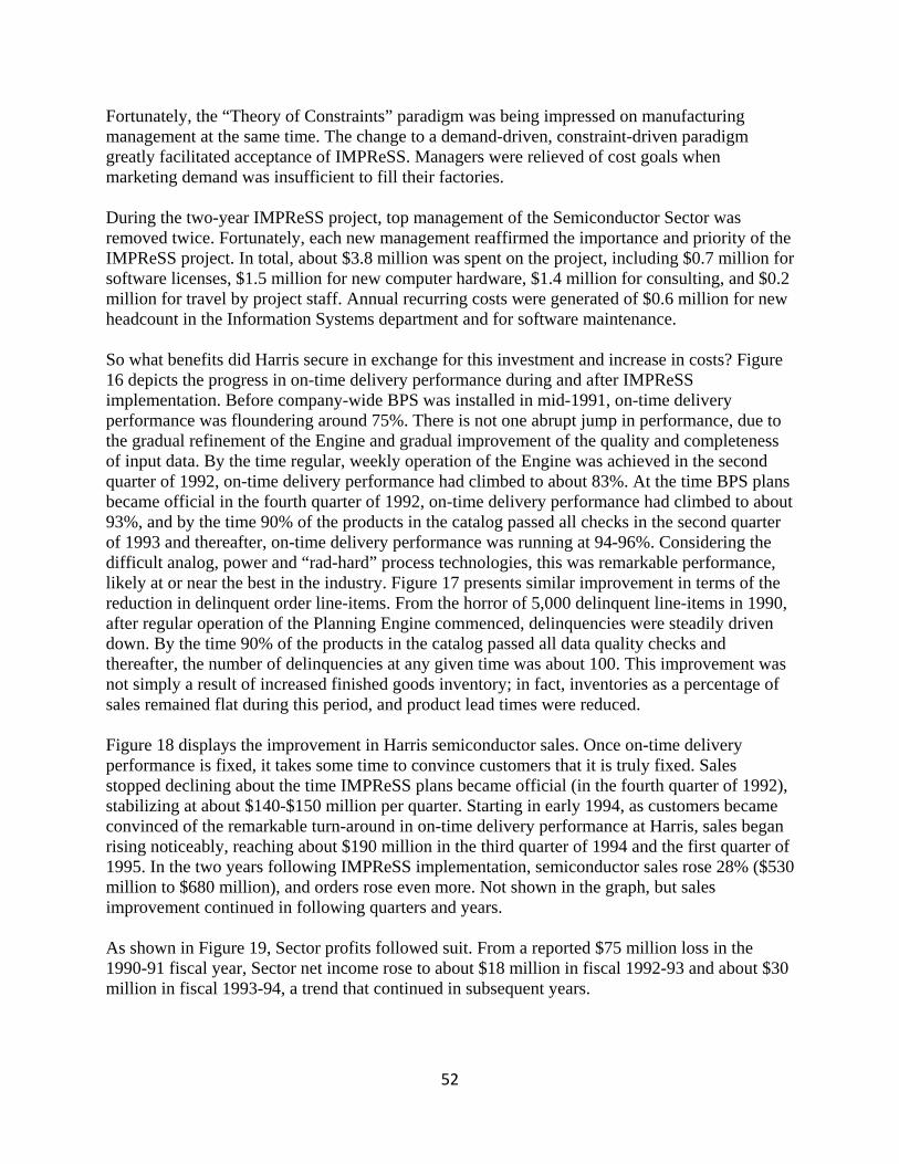
52
Fortunately, the “Theory of Constraints” paradigm was being impressed on manufacturing management at the same time. The change to a demand-driven, constraint-driven paradigm greatly facilitated acceptance of IMPReSS. Managers were relieved of cost goals when marketing demand was insufficient to fill their factories. During the two-year IMPReSS project, top management of the Semiconductor Sector was removed twice. Fortunately, each new management reaffirmed the importance and priority of the IMPReSS project. In total, about $3.8 million was spent on the project, including $0.7 million for software licenses, $1.5 million for new computer hardware, $1.4 million for consulting, and $0.2 million for travel by project staff. Annual recurring costs were generated of $0.6 million for new headcount in the Information Systems department and for software maintenance. So what benefits did Harris secure in exchange for this investment and increase in costs? Figure 16 depicts the progress in on-time delivery performance during and after IMPReSS implementation. Before company-wide BPS was installed in mid-1991, on-time delivery performance was floundering around 75%. There is not one abrupt jump in performance, due to the gradual refinement of the Engine and gradual improvement of the quality and completeness of input data. By the time regular, weekly operation of the Engine was achieved in the second quarter of 1992, on-time delivery performance had climbed to about 83%. At the time BPS plans became official in the fourth quarter of 1992, on-time delivery performance had climbed to about 93%, and by the time 90% of the products in the catalog passed all checks in the second quarter of 1993 and thereafter, on-time delivery performance was running at 94-96%. Considering the difficult analog, power and “rad-hard” process technologies, this was remarkable performance, likely at or near the best in the industry. Figure 17 presents similar improvement in terms of the reduction in delinquent order line-items. From the horror of 5,000 delinquent line-items in 1990, after regular operation of the Planning Engine commenced, delinquencies were steadily driven down. By the time 90% of the products in the catalog passed all data quality checks and thereafter, the number of delinquencies at any given time was about 100. This improvement was not simply a result of increased finished goods inventory; in fact, inventories as a percentage of sales remained flat during this period, and product lead times were reduced. Figure 18 displays the improvement in Harris semiconductor sales. Once on-time delivery performance is fixed, it takes some time to convince customers that it is truly fixed. Sales stopped declining about the time IMPReSS plans became official (in the fourth quarter of 1992), stabilizing at about $140-$150 million per quarter. Starting in early 1994, as customers became convinced of the remarkable turn-around in on-time delivery performance at Harris, sales began rising noticeably, reaching about $190 million in the third quarter of 1994 and the first quarter of 1995. In the two years following IMPReSS implementation, semiconductor sales rose 28% ($530 million to $680 million), and orders rose even more. Not shown in the graph, but sales improvement continued in following quarters and years. As shown in Figure 19, Sector profits followed suit. From a reported $75 million loss in the 1990-91 fiscal year, Sector net income rose to about $18 million in fiscal 1992-93 and about $30 million in fiscal 1993-94, a trend that continued in subsequent years.

53
Figure 16. Improvement in On-Time Delivery Performance at Harris Corporation – Semiconductor Sector
Source: Leachman et al [1996].
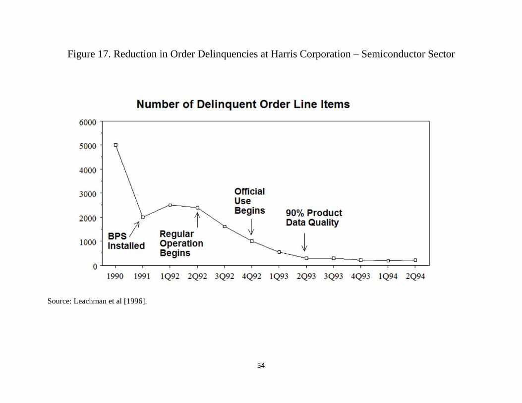
54
Figure 17. Reduction in Order Delinquencies at Harris Corporation – Semiconductor Sector
Source: Leachman et al [1996].

55
Figure 18. Improvement in Sales at Harris Corporation – Semiconductor Sector
Source: Leachman et al [1996].
56
Figure 19. Improvement in Net Income at Harris Corporation – Semiconductor Sector
Source: Leachman et al [1996].
Sector Net Income
57
As a result of IMPReSS, Harris observed many benefits. Product lead times and manufacturing cycle times were reduced. The improved on-time delivery performance enabled Harris to penetrate new markets; for example, after IMPReSS, Harris was able to make major sales into the Japanese telecommunications equipment market, a market they had not been able to sell into beforehand. The substantial increase in centralized data and data maintenance enabled other business processes to improve. For example, data concerning equipment process times for the various products enabled cost accounting improvements and improved pricing decisions. The Cost Accounting Department became a strong champion of maintenance of the IMPReSS capacity databases. In addition to on-line planning for establishing factory schedules and product availability, the IMPReSS software was utilized in off-line planning supporting capital planning and budgeting decisions. Before IMPReSS, equipment acquisition plans for fabrication and probe areas and for assembly and test areas were prepared independently. After IMPReSS, a company-wide analysis became feasible. For example, to realize the gains from purchasing a number of testers, a new ion implanter for a fabrication area also needed to be purchased. Considering the lead time to secure a new implanter, the timing of the purchase of the testers needed to be delayed. This led to much wiser capital spending decisions. President Farmer of Harris testified that the first-year savings in equipment purchases exceeded the cost of the entire IMPReSS project by a wide margin. IMPReSS provided an integrated, globally optimized production plan, replacing local optimization efforts. In general, IMPReSS enabled a global, common understanding of demands and constraints at the Semiconductor Sector of Harris. Other semiconductor companies were amazed at the level of communication and coordination between front-end (fabrication and probe) plants and back-end (assembly and test) plants. In 1995, the IMPReSS project was nominated for the Franz Edelman Award Competition. The Edelman Award is given annually by the Institute for Operations Research and the Management Sciences (INFORMS) recognizing outstanding industrial practice of the management sciences. The IMPReSS project won the competition. This was a fitting honor; Franz Edelman was one of the first three Operations Research PhDs from MIT and the Director of the Operations Research Dept. at RCA Corporation. Years later after Edelman’s retirement, RCA’s semiconductor business, which Edelman’s department had done much to improve in its early years, was part of the Harris Semiconductor business now recognized for carrying on his tradition. Rather than dying, the Semiconductor business of Harris survived and even thrived. In 1999, it was spun off from Harris as a new company with an old name – Intersil. The initial public offering raised more than $1 billion, the largest IPO in semiconductor industry history. In the wake of the Edelman Award, the basic BPS and IMPReSS methodologies were published in the open literature. Most semiconductor companies worked to integrate and automate their supply chain management. The typical strategy pursued was to integrate one of the generic ERP systems with an advanced planning engine. At least five vendors of advanced planning engines specially designed for the semiconductor industry began marketing their products to the industry, some optimization-based, others incorporating rule-based logic, constraint satisfaction and/or
58
artificial intelligence. All claimed to incorporate the important features pioneered in BPS. In the author’s opinion, none of them matched the capabilities of BPS. The IMPReSS system continued to run at Harris and then Intersil until 2004, a span of 12 years, when it was replaced by one of the commercial systems. The BPS software or precedents developed at U. C. Berkeley also saw application in other companies, including Intel, Advanced Micro Devices, Samsung, Cypress Semiconductor, and Micron Technology. References 1. Hung, Yi-Feng and R. C. Leachman, 1996. "A Production Planning Methodology for Semiconductor Manufacturing Based on Iterative Simulation and Linear Programming Calculations," EEE Transactions on Semiconductor Manufacturing, 9 (2), p. 257-269 (May, 1996). 2. Leachman, Robert C., 1993. “Modeling techniques for automated production planning in the semiconductor industry,” Optimization in Industry, T. A. Ciriani and R. C. Leachman, editors, John Wiley and Sons, Ltd., Chichester, England, p. 1-30. 3. Leachman, Robert C., 2001. "Semiconductor Production Planning," in Handbook of Applied Optimization, Panos M. Pardalos and Mauricio G. C. Resende (Eds.), Oxford University Press, New York, p. 746-762 (2001). 4. Leachman, Robert C., R. F. Benson, D. J. Raar and C. Liu, 1996. "IMPReSS: An Automated Production Planning and Delivery Quotation System at Harris Corporation - Semiconductor Sector," Interfaces, 26 (1), p. 6-37 (Jan – Feb, 1996). 5. Leachman Robert C., and Tali F. Carmon, 1992. "On Capacity Modeling for Production Planning With Alternative Machine Types," IIE Transactions, 24 (4), p. 62-72 (September, 1992). 6. Lin, Vincent, 1999. Advanced Semiconductor Production Planning, PhD Thesis, College of Engineering, University of California at Berkeley, Berkeley, CA.
Related Documents