Country risk ratings and financial crises 1995 – 2001: a survival analysis

- Bogotá - Colombia - Bogotá - Colombia - Bogotá - Colombia - Bogotá - Colombia - Bogotá - Colombia - Bogotá - Colombia - Bogotá - Colombia - Bogotá - Colombia - Bogotá -

Country risk ratings and financial crises 1995 - 2001: a survival analysis Por: Leonardo Bonilla, Andrés Felipe García, Mónica Roa

No. 4992008

Country risk ratings and financial crises 1995 – 2001: a

survival analysis

Leonardo Bonilla♣

Andrés Felipe García♦ & Mónica Roa†

Abstract Financial system’s health is a signal of economic growth therefore it is a key indicator to investors. As a consequence, one of the main purposes of policymakers is to keep its stability as well as protect it from foreign activity. Both financial and economic activity in general are susceptible of crises, as soon as this happen a country may face default risk, which can be measured with long term debt risk rating of countries. Through this variable we propose the use the survival analysis methodology, to analyze falls rating duration and capability of macroeconomic variables to predict that event. From the analysis, we point out important differences between developed and emerging economies, with variables which stand out exchange risk and economies indebtedness.

Resumen La dinámica del sistema financiero es una señal de crecimiento económico, por lo tanto es un indicador clave para los inversionistas. Por lo tanto, uno de los principales retos de la política económica es mantener la estabilidad así como proteger el sistema financiero de los fenómenos externos. La actividad financiera y la actividad económica son en general susceptibles a las crisis y dicho riesgo puede medirse a partir de la calificación de deuda de largo plazo. A través de esta variable proponemos aplicar el análisis de sobrevivencia, para explorar la duración de las caídas en la calificación de riesgo y la capacidad de variables macroeconómicas para predecirlas. Con ello se encontraron diferencias importantes en las economías desarrolladas y emergentes, teniendo en cuenta variables de riesgo cambiario y endeudamiento de la economía.

♣ Universidad Nacional de Colombia, research intern at Banco de la República. ♦ Researcher Universidad del Rosario, research intern at Banco de la República in 2006. † Researcher Universidad del Rosario. Contact information: [email protected] [email protected] [email protected] We thank José Eduardo Gomez, Jeffrey Wilson and Constanza Martinez for their useful comments. All errors remain ours.

2

Classification JEL: G15, G28, H81. Key words: financial crises, financial risk, foreign debt, survival models.

INTRODUCTION

As the world globalizes, financial stability is one of the main concerns all over the

world. Moreover, if one takes into account both financial system’s vulnerability to

foreign markets and its stability are a signal to investors, therefore bad behavior of the

system do not contribute to economic growth. A key indicator of the domestic capital

market’s health is the credit rating given to the long term debt, which gives information

of short term macroeconomic stability and payment capability at long term. Indeed, as

Ratha (2008) states “sovereign risk ratings from agencies such as Fitch, Moody’s, and

Standard and Poor’s affect capital flows to developing countries through international

bond, loan and equity markets. Sovereign rating also acts as a ceiling for the foreign

currency rating of sub-sovereign borrowers”.

Because of what was pointed out above, the present paper presents an approximation to

financial crises through sovereign risk ratings. Our analysis presents two important

aspects in rating falls, which were not considered before in this kind of analysis:

country’s effect and falls timing; to attain these points we propose the use of a survival

model. This paper uses this methodology to compute the risk function of a fall rating

controlling by macroeconomics and exchange monthly variables which reflect

economics’ health at short and mid term for 78 countries between 1995 and 20011. We

exclude from the analysis variables from the real sector as they may be endogenous with

country risk rating.

Authors who analyses sovereign ratings (Haque et al.: 1998, Reinhart, 2001, 2002)

focus on its determinants. This study offers a step forward by analyzing determinants in

time with a survival model, which was not used before in this kind of studies. This

methodology also allows us to forecast crisis duration and contagion by geographic and

economic regions. In the study we use a semiparametric methodology, which is better in

the analysis of non-monotonic risk functions given the persistence and contagion effect.

1 This period in which there were a world crisis, sovereign ratings changed as economic country conditions changed, these facts allows us the use of survival analysis

3

The paper is divided into six sections, the first is this introduction; the second is a short

reference to some hypothesis and theory about financial crises; the third one

summarizes the methodology; the fourth section presents the nonparametric survival

analysis based on risk functions; the fifth section includes the results, and the sixth is

the conclusion.

RELATED LITERATURE

As Eichengreen (1999) emphasizes, financial crisis are not new; the difference is their

violence and the damage they do. According with its time, connoisseurs catalog crisis in

three generations.

The first generation model, which was used to explain crises in the early 1980s, were

based on the macroeconomic imbalances. To support this point, Krugman (1979) uses a

simple model to show how attempts to defend a fixed exchange rate can collapse in the

face of a speculative attack. He shows how the persistence balance of payments deficits2

can push a run on the authorities’ stock of international reserves and destroy their

capacity to defend the exchange rate by sticking up the ability to intervene in the

foreign-exchange market. The central point of this generation studies is to demonstrate

how an attack collapsing the exchange rate can occur before reserves would have been

exhausted otherwise and to pin down its timing. As the point here is that government

exhausted the reserves and they cannot replenish them by borrowing abroad, the leading

indicators of this generation of crisis are budget deficits, excessive rates of growth of

money supply and dwindling reserves. Countries that are susceptible to speculative

attacks may also exhibit excessive inflation, real exchange rate overvaluated and rising

interest rates.

With the crisis of the early 1990s, the above symptoms were questioned, because not all

the countries that succumbed, displayed large fiscal and current account deficits. In

addition, as control to capitals were lifted and international markets growed, it was less

possible to assume that central banks could not borrow abroad to replenish their

2 Krugman assumed that payments imbalances and the currency crisis resulted from the tendency of governments to run expansionary monetary and fiscal policies, which are financed by printing money.

4

reserves. Obstfeld (1997) and Ozkan and Sutherland (1998) add the assumption that

governments balance the benefits of continuing to defend the currency through tight

monetary policies and high interest rates. Under these assumptions, authorities enhance

their commitment to defend the currency and to maintain price stability, but the impact

of high interest rates on the economy and the financial system are so high. Although

there are no restrictions to capital, in these second generation models the level of

reserves and the ability to get money abroad play no role in calculations. The issue here

is the role played by interest rates to defend currency and therefore, its impact on

depressing demand on the default of bank borrowers and on a large short term debt. The

decision of defending the currency came up from an economic and political self-

interest. Actually, by observing ninety-one countries over the period 1960-1996,

Gourinchas et al. (2001) found that probability of a bank of exchange crisis increases

once the country decides to adopt liberalization as a policy. They notice this may be due

to an absence of regulation or to partial liberalizations based on exchange measures and

not on monetary policies. Reinhart (2001) revalues liberalization notion by standing out

the need of protect domestic finances from capital flows fluctuations. Thus, in second

generation models the crisis depends on subtler unmeasured conditions such as the

strength of the banking system, or labor market flexibility, or the prospects of economic

growth and domestic political support to the government and its policies. In fact Calvo

and Reinhart (1996) prove that contagion mechanism is related with a fixed exchange

rate and high interest rates, and contrary of what may be thought its impact is the same

whether small or big countries. Indeed contagion effect occurs easier at a regional level

than in a global one, meaning affected countries not only belong to a specific

geographical region but also to a specific group.

Finally, the main differences between first and second generation models is that in the

latter the speculative attack can precipitate a devaluation that would not have occurred

in its absence; and that capital controls can bend the balance between the collapse of the

currency peg and its maintenance forever3. Therefore an attack that would have neither

occurred nor succeeded in the presence of capital controls may do both in their absence.

3 As in the absence of capital control restrictions, domestic interest rates equal foreign interest rate plus the expected rate of depreciation.

5

The crisis of the late 1990s came up with the third generation models. Based on the

facts observed in Asia, where there were combined issues from the first and second

generation models, connoisseurs pointed out that those models have something that was

missing. Additionally, by using data from more than seventy countries during 1960-

2000, Loaiza and Ranciere (2005) states that economic growth might be negative if the

country faces a weak financial system in a maturation process due to moral hazard and

incentive problems. Because of these new conclusions, connoisseurs proposed the third

generation models which were called crony capitalism and implicit guarantees.

Basically it was a moral hazard problem in which owners of banks and industrial

conglomerates on one side, and political leaders on the other, develop ties of mutual

dependence which left governments loath to let banks fail (Dooley: 1997 and Krugman:

1998 in Eichengreen: 1999). Once the capital account of the balance of payments was

opened, the implicit guarantees provided by government to banks were a lure to foreign

investors and with governments guaranteeing banks against failure, the specter of losses

was removed therefore, foreign capital flooded the economy and banking system.

Mackinnon and Pill (1997) argue that once this happened foreign borrowing was so

excessive and funds were so poorly allocated that capital inflow may reduce the growth

rates of the countries involved. Therefore the initial capital outflow with the problem

that governments’ guarantees can be provided only once, therefore, the relationship

between bankers and politicians’ guarantees provoked a populist backlash that brought

the crony capitalism. As the authorities leapt to the rescue of the banking system,

pumping in additional domestic credit, they were forced to disregard the constraints on

liquidity implied by the commitment to peg the exchange rate.

Finally there are some authors who have focused in studying all three generations

models by using whether a subjective definition of crisis (Manasse et. al.: 2003) or by

seeing the correlation between credit ratings and crisis episodes (Reinhart: 2002)

especially in Asia and Argentina. On a first sight both perspectives use macroeconomics

and political variables to check the influence on the dependent variable (crisis or credit

rating). On the other hand the authors who use ratings found not only an amazing

correlation between the credit rating and sovereign default but they also found that the

key determinants of ratings are macroeconomic variables meanwhile political variables

have a marginal effect (Haque et. al.: 1998, Bissoondoyal-Bheenick, 2005). In addition,

6

they found a pattern in country crises by pointing out that for most of the sample they

studied previous to the debt crisis there was a currency crisis.

SURVIVAL ANALYSIS

Probability models have been the most used methodology to study the determinants of

change. Later studies point out that the analysis allows the advance in mathematical and

statistical tools.

The first empirical studies reckoned the probability of leaving the current state by

explaining the individual characteristics at a specific moment based on binary models4

in which the probability of maintaining the current state or changing. Thought, this

method is a static approximation which does not capture nor temporality or deviation

from circumstances which may affect the conditional probability of change. Therefore,

by using this methodology it is not possible to answer questions such as: is there any

point in time in which the chance of change is higher? or which is the probability of

change the state given that the agent has been active until the present period?

Survival models are not only focused on the occurrence of the event, but also on the

impact of predictable variables (constant or changing in time)5 on the chance of change

the state. The dynamic method which takes account time and individual characteristics

depend on elements which are seen by traditional literature as specification errors,

which do not allow an efficient estimation and, therefore, probabilities may be

underestimated or overestimated. These elements may be summarized as: censoring,

continuous or discrete treatment, ties and multiple causes of ending.

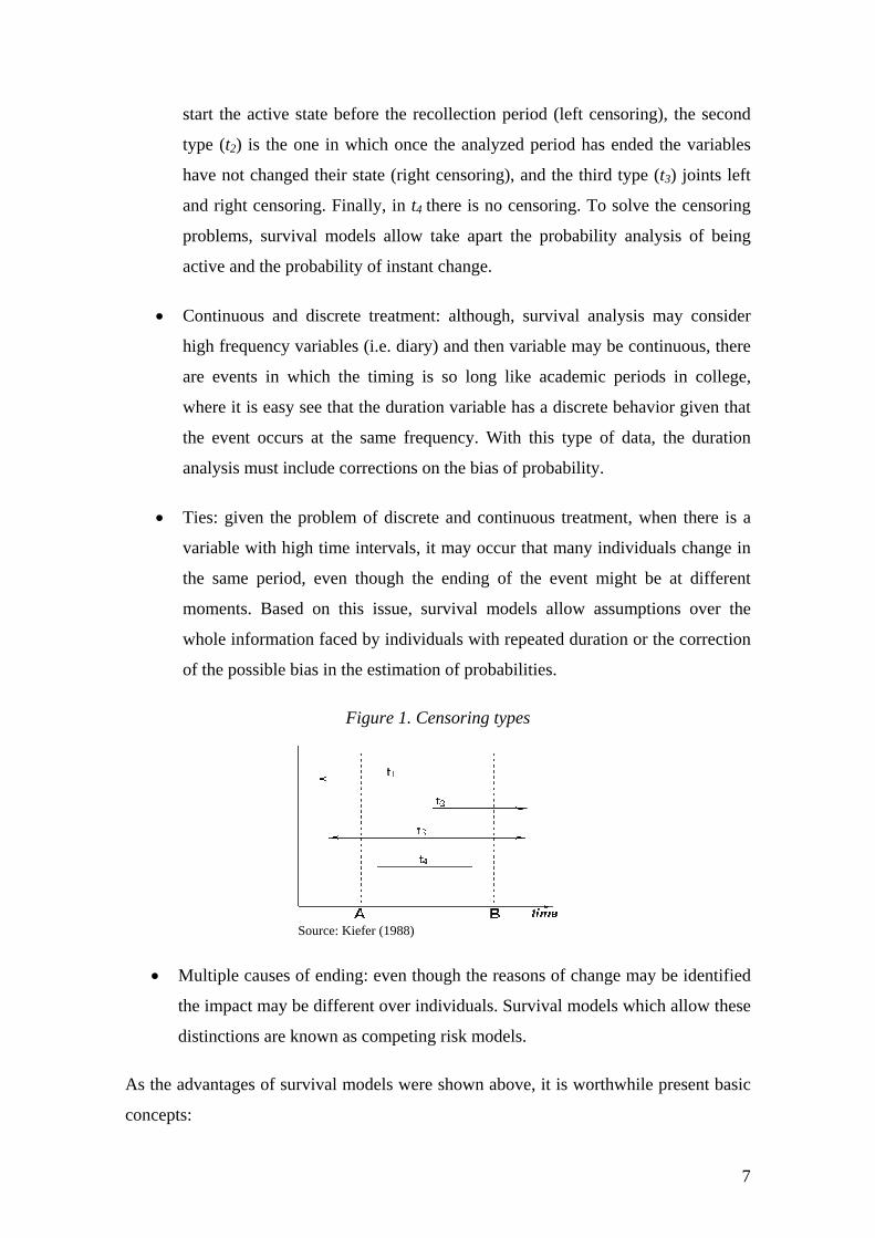
• Censoring: an observation is censored when it does not change in the analyzed

period. Based on this fact one may define three types of censoring which are

presented in Figure 1, the first (t1) makes reference to those observations which 4 In these models, the values of the dependent variable are 0 and it follows a particular distribution, the most commonly used are the logistic and the normal standard distributions 5 The inclusion of changing variables may cause simultaneity or autocorrelation.

7

start the active state before the recollection period (left censoring), the second

type (t2) is the one in which once the analyzed period has ended the variables

have not changed their state (right censoring), and the third type (t3) joints left

and right censoring. Finally, in t4 there is no censoring. To solve the censoring

problems, survival models allow take apart the probability analysis of being

active and the probability of instant change.

• Continuous and discrete treatment: although, survival analysis may consider

high frequency variables (i.e. diary) and then variable may be continuous, there

are events in which the timing is so long like academic periods in college,

where it is easy see that the duration variable has a discrete behavior given that

the event occurs at the same frequency. With this type of data, the duration

analysis must include corrections on the bias of probability.

• Ties: given the problem of discrete and continuous treatment, when there is a

variable with high time intervals, it may occur that many individuals change in

the same period, even though the ending of the event might be at different

moments. Based on this issue, survival models allow assumptions over the

whole information faced by individuals with repeated duration or the correction

of the possible bias in the estimation of probabilities.

Figure 1. Censoring types

Source: Kiefer (1988)

• Multiple causes of ending: even though the reasons of change may be identified

the impact may be different over individuals. Survival models which allow these

distinctions are known as competing risk models.

As the advantages of survival models were shown above, it is worthwhile present basic

concepts:

8

The first remark must be made on the dependent variable; the duration variable must be

a random nonegative variable, thus it may be represented by density function )(tf and

by a cumulative distribution function ( )tTPtF ≤=)( . The first function is related to the

duration of the event and the second is related to the maximum duration.

Based on the functions mentioned above, one constructs the survival and the risk

functions. The first function captures the probability that an individual lasts more than a

specific time, which may be assessed by the survival function ( ) ( )tTPtFtS ≥=−= )(1 .

The risk or hazard function, represents the instant probability of change, it means it

considers the duration between the active stage and when it ends, and this may be

represented as ( ) ( ) ( ) ( )( )tStftTtftTttTtPth =≥=≥∆+<≤= .

The purpose of survival models is to assess ( )tS and ( )th based on the observed

individual characteristics, to achieve it there are two kinds of survival methodologies:

parametric and nonparametric estimations. To obtain ( )tS , the methodology used is the

proposed by Kaplan and Meier (1958), which is based on the nonparametric estimators

of product limit, the most efficient estimator. The Kaplan-Meier estimator is given by:

( )⎪⎩

⎪⎨

⎧

≥⎟⎟⎠

⎞⎜⎜⎝

⎛−

<

=∏≤tt i

i

i

ttifyd1

ttif1tS

Where t is the period in which the first change occurs, iy is the sum of individuals who

may change of state at moment it and id is the number of individuals who change at

moment it .

Based on the survival function, one may get the cumulative risk function ( )tΛ meaning

the cumulative risk at specific moment; this is known as the Nelson-Aalen estimator,

which accomplishes with the Kaplan-Meiers’s estimator properties. The estimator is

denoted by:

( )⎪⎩

⎪⎨

⎧

≥

<=Λ ∏

≤tt i

i

i

ttifyd

ttif0tˆ

9

With ( )tΛ , one gets the instant probability of change; this is a raw nonparametric

estimator of the risk function; given by:

( ) ( ) ( )1ˆˆˆ −Λ−Λ=Λ∆ ttt

An estimation of the smooth risk function may be made by a kernel approximation

of ( )tΛ∆ ˆ . Risk function may be achieved by using, either parametric or semiparametric

estimators: the first estimators are based on the assumption that duration depends on a

monotonous way from the probability of change with weibull, exponencial or gompertz

distributions. The latest group estimators assumes that relation between survival and

probability may has a nonmonotonic form, which is an advantage, not only because this

more general but also because estimators are more efficient.

As in the present paper we use semiparametric estimators, we focus on some

specifications on them. The pioneer model is the one proposed by Cox (1972); this

assumes that risk function has a multiplicative form which allows split time effect and

the probability (baseline hazard) which captures the common risk of individuals at

specific time and the effect that depends on individual characteristics which is defined

by a nonnegative function, by simplicity one assumes this function as an indicator

exponential function, which is a lineal combination of individual characteristics. Then

the Cox model can be summarizing in the function6:

( ) ( ) βiethth ixx ′= 0

Where ( )th0 is the common risk function or baseline and βiex′ is the function which

points out individual characteristics´ effect on probability of change.

DATA AND NONPARAMETRIC ESTIMATION

The paper analyzes information of 78 countries between 1995 and 2001. Because of

asymptotic properties of the models we use and the frequency of independent variables

data frequency is monthly. The countries chosen were those which have sovereign risk

rating during the studied period. The sample is representative among countries with

6 One of the advantages of this approximation to the risk function is that it accomplishes the independence irrelevant alternative assumption, because risk relative function risk depends only on the individual characteristics.

10

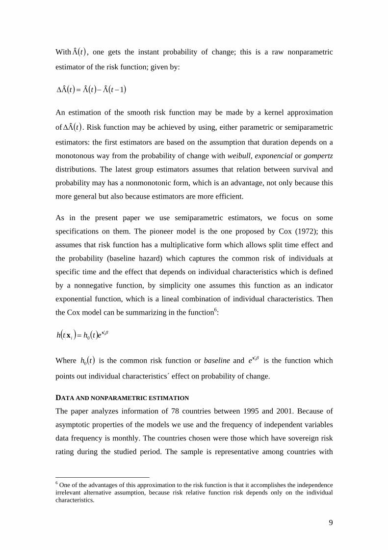
capital markets more or less developed. Ratings are classified by region and by OECD

members, as can be seen in Figure 2:

Figure 2. Number of countries by region and OECD

0

10

2030

40

50

6070

80

90

Africa America AsiaOceanía

Europa Totalgeneral

NO OECD OECD Total

The variable we use to assess risk country is the rating given by the agency Moody to

long term bond in foreign currency. The ratings go up from Aaa to C, with numeric

variations from 1 to 3 and; + or – signs if the changes were minimal. By observing data

ratings, we notice that meanwhile ratings higher or equal to Baa3 belong to investment

scale and, lower or equal ratings to Ba1 are in speculation scale. In the analysis every

fall rating is a default. In the analyzed period there were 72 ratings fall, the region with

more failures is Asia Pacific, followed by America and Europe. Although African

countries ratings do not fall, they confer information to survival function; therefore

African information must be included. Figure 3 presents failure distribution by OECD

country and region.

In contrast to other risk indicators, country risk rating from the agency Moody’s not

only takes account economic variables in a pure sense but also considers long term

issues. Although literature does not make difference between crisis and country’s

decline, we must call attention to one point: we define default as any fall rating. By

doing this we avoid subjective definitions of crisis like those proposed by Domaç and

Martinez (2000) and Gourinchas et al. (2001) and we make use of the above mentioned

ratings’ characteristics.

11

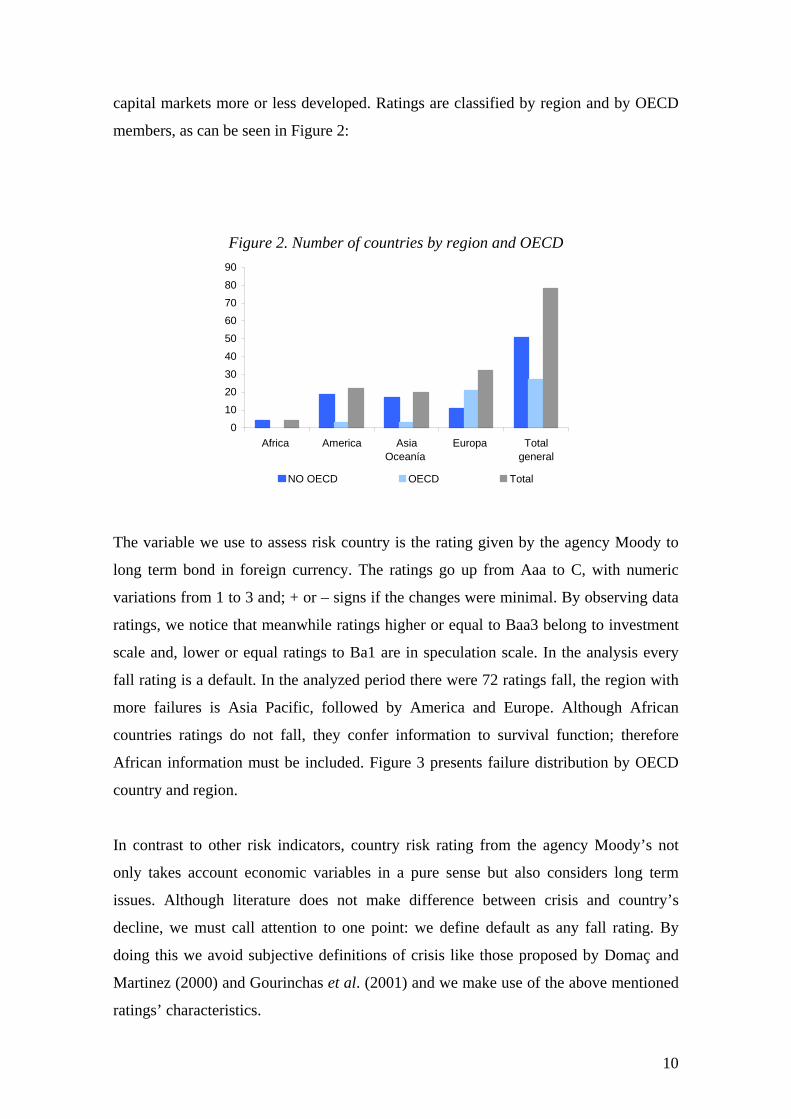
In the analysis every fall rating is a default. In the analyzed period there were 72 ratings

fall, the region with more failures is Asia Pacific, followed by America and Europe.

Figure 3. Number of sovereign risk rating falls by region and OECD

0

10

20

30

40

50

60

70

80

Africa America Asia Oceanía Europa Total general

NO OECD OECD Total

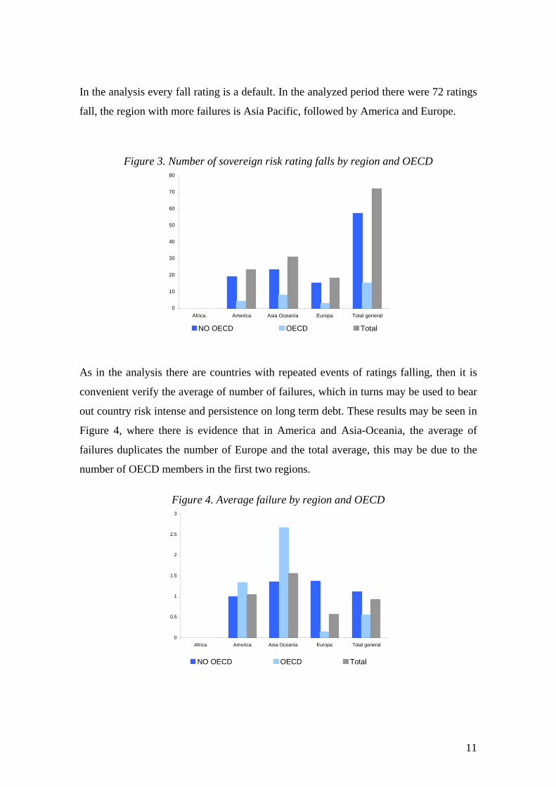
As in the analysis there are countries with repeated events of ratings falling, then it is

convenient verify the average of number of failures, which in turns may be used to bear

out country risk intense and persistence on long term debt. These results may be seen in

Figure 4, where there is evidence that in America and Asia-Oceania, the average of

failures duplicates the number of Europe and the total average, this may be due to the

number of OECD members in the first two regions.

Figure 4. Average failure by region and OECD

0

0.5

1

1.5

2

2.5

3

Africa America Asia Oceanía Europa Total general

NO OECD OECD Total

12

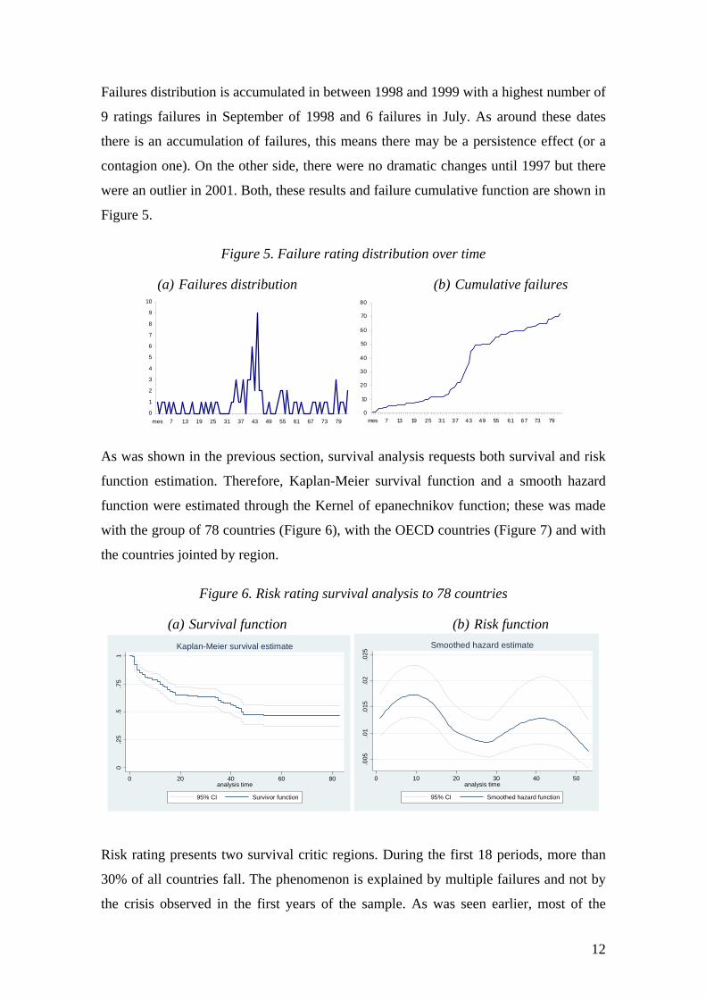
Failures distribution is accumulated in between 1998 and 1999 with a highest number of

9 ratings failures in September of 1998 and 6 failures in July. As around these dates

there is an accumulation of failures, this means there may be a persistence effect (or a

contagion one). On the other side, there were no dramatic changes until 1997 but there

were an outlier in 2001. Both, these results and failure cumulative function are shown in

Figure 5.

Figure 5. Failure rating distribution over time

(a) Failures distribution (b) Cumulative failures

0

1

2

3

4

5

6

7

8

9

10

mes 7 13 19 25 31 37 43 49 55 61 67 73 790

10

20

30

40

50

60

70

80

mes 7 13 19 25 31 37 43 49 55 61 67 73 79

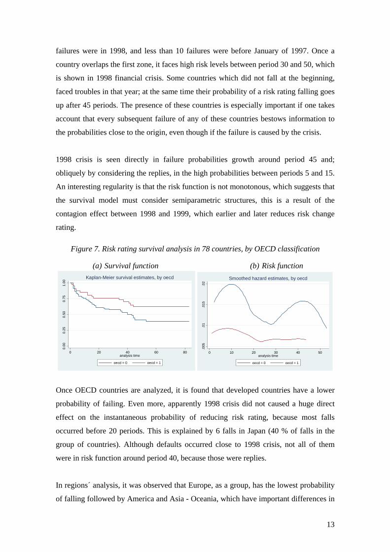
As was shown in the previous section, survival analysis requests both survival and risk

function estimation. Therefore, Kaplan-Meier survival function and a smooth hazard

function were estimated through the Kernel of epanechnikov function; these was made

with the group of 78 countries (Figure 6), with the OECD countries (Figure 7) and with

the countries jointed by region.

Figure 6. Risk rating survival analysis to 78 countries

(a) Survival function (b) Risk function

0.2

5.5

.75

1

0 20 40 60 80analysis time

95% CI Survivor function

Kaplan-Meier survival estimate

.005

.01

.015

.02

.025

0 10 20 30 40 50analysis time

95% CI Smoothed hazard function

Smoothed hazard estimate

Risk rating presents two survival critic regions. During the first 18 periods, more than

30% of all countries fall. The phenomenon is explained by multiple failures and not by

the crisis observed in the first years of the sample. As was seen earlier, most of the

13

failures were in 1998, and less than 10 failures were before January of 1997. Once a

country overlaps the first zone, it faces high risk levels between period 30 and 50, which

is shown in 1998 financial crisis. Some countries which did not fall at the beginning,

faced troubles in that year; at the same time their probability of a risk rating falling goes

up after 45 periods. The presence of these countries is especially important if one takes

account that every subsequent failure of any of these countries bestows information to

the probabilities close to the origin, even though if the failure is caused by the crisis.

1998 crisis is seen directly in failure probabilities growth around period 45 and;

obliquely by considering the replies, in the high probabilities between periods 5 and 15.

An interesting regularity is that the risk function is not monotonous, which suggests that

the survival model must consider semiparametric structures, this is a result of the

contagion effect between 1998 and 1999, which earlier and later reduces risk change

rating.

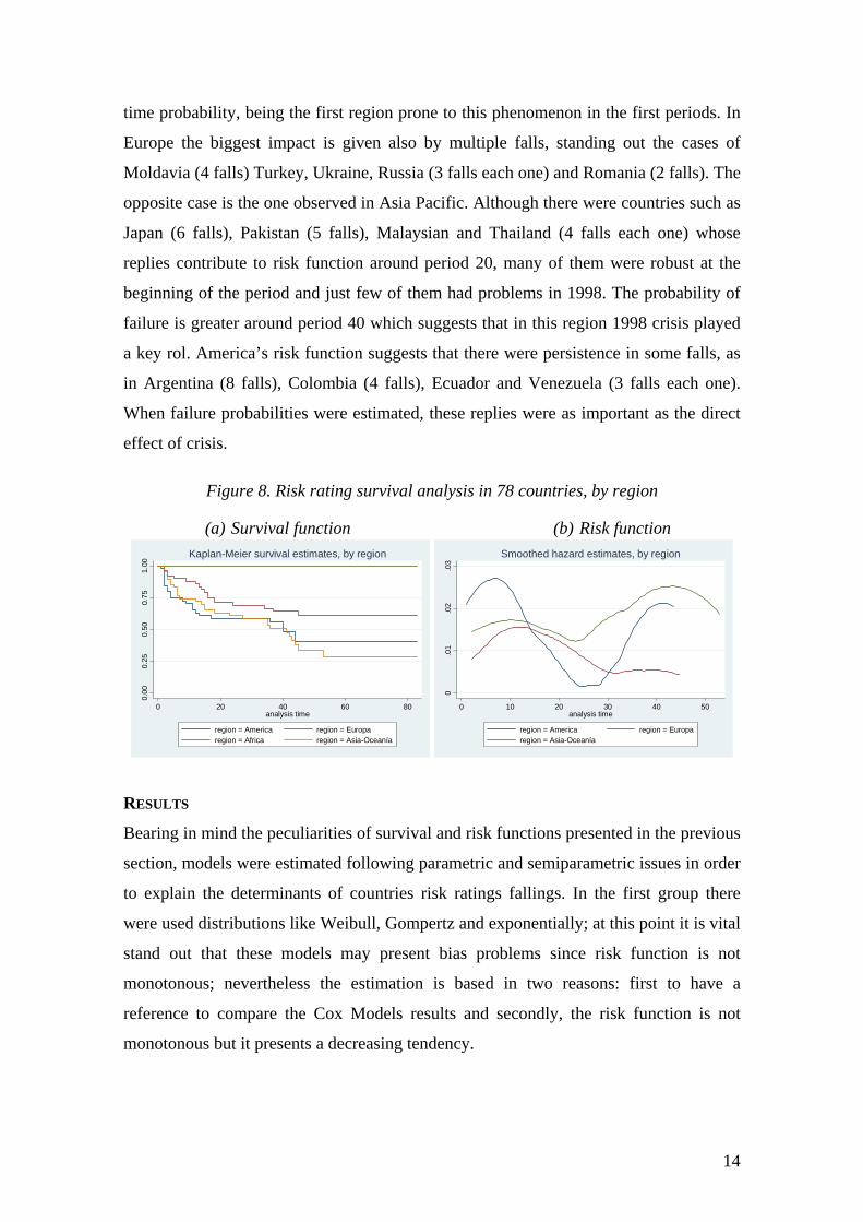
Figure 7. Risk rating survival analysis in 78 countries, by OECD classification


0.00

0.25

0.50

0.75

1.00


oecd = 0 oecd = 1

Kaplan-Meier survival estimates, by oecd

.005

.01

.015

.02


oecd = 0 oecd = 1

Smoothed hazard estimates, by oecd

Once OECD countries are analyzed, it is found that developed countries have a lower

probability of failing. Even more, apparently 1998 crisis did not caused a huge direct

effect on the instantaneous probability of reducing risk rating, because most falls

occurred before 20 periods. This is explained by 6 falls in Japan (40 % of falls in the

group of countries). Although defaults occurred close to 1998 crisis, not all of them

were in risk function around period 40, because those were replies.

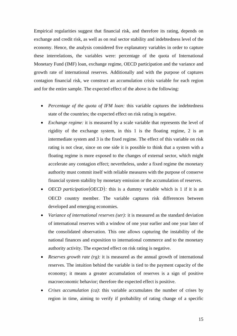
In regions´ analysis, it was observed that Europe, as a group, has the lowest probability

of falling followed by America and Asia - Oceania, which have important differences in

14

time probability, being the first region prone to this phenomenon in the first periods. In

Europe the biggest impact is given also by multiple falls, standing out the cases of

Moldavia (4 falls) Turkey, Ukraine, Russia (3 falls each one) and Romania (2 falls). The

opposite case is the one observed in Asia Pacific. Although there were countries such as

Japan (6 falls), Pakistan (5 falls), Malaysian and Thailand (4 falls each one) whose

replies contribute to risk function around period 20, many of them were robust at the

beginning of the period and just few of them had problems in 1998. The probability of

failure is greater around period 40 which suggests that in this region 1998 crisis played

a key rol. America’s risk function suggests that there were persistence in some falls, as

in Argentina (8 falls), Colombia (4 falls), Ecuador and Venezuela (3 falls each one).

When failure probabilities were estimated, these replies were as important as the direct

effect of crisis.

Figure 8. Risk rating survival analysis in 78 countries, by region


0.00

0.25

0.50

0.75

1.00


region = America region = Europaregion = Africa region = Asia-Oceanía

Kaplan-Meier survival estimates, by region

0.0

1.0

2.0

3


region = America region = Europaregion = Asia-Oceanía

Smoothed hazard estimates, by region

RESULTS

Bearing in mind the peculiarities of survival and risk functions presented in the previous

section, models were estimated following parametric and semiparametric issues in order

to explain the determinants of countries risk ratings fallings. In the first group there

were used distributions like Weibull, Gompertz and exponentially; at this point it is vital

stand out that these models may present bias problems since risk function is not

monotonous; nevertheless the estimation is based in two reasons: first to have a

reference to compare the Cox Models results and secondly, the risk function is not

monotonous but it presents a decreasing tendency.

15

Empirical regularities suggest that financial risk, and therefore its rating, depends on

exchange and credit risk, as well as on real sector stability and indebtedness level of the

economy. Hence, the analysis considered five explanatory variables in order to capture

these interrelations, the variables were: percentage of the quota of International

Monetary Fund (IMF) loan, exchange regime, OECD participation and the variance and

growth rate of international reserves. Additionally and with the purpose of captures

contagion financial risk, we construct an accumulation crisis variable for each region

and for the entire sample. The expected effect of the above is the following:

• Percentage of the quota of IFM loan: this variable captures the indebtedness

state of the countries; the expected effect on risk rating is negative.

• Exchange regime: it is measured by a scale variable that represents the level of

rigidity of the exchange system, in this 1 is the floating regime, 2 is an

intermediate system and 3 is the fixed regime. The effect of this variable on risk

rating is not clear, since on one side it is possible to think that a system with a

floating regime is more exposed to the changes of external sector, which might

accelerate any contagion effect; nevertheless, under a fixed regime the monetary

authority must commit itself with reliable measures with the purpose of conserve

financial system stability by monetary emission or the accumulation of reserves.

• OECD participation ( )OECD : this is a dummy variable which is 1 if it is an

OECD country member. The variable captures risk differences between

developed and emerging economies.

• Variance of international reserves (ser): it is measured as the standard deviation

of international reserves with a window of one year earlier and one year later of

the consolidated observation. This one allows capturing the instability of the

national finances and exposition to international commerce and to the monetary

authority activity. The expected effect on risk rating is negative.

• Reserves growth rate (rg): it is measured as the annual growth of international

reserves. The intuition behind the variable is tied to the payment capacity of the

economy; it means a greater accumulation of reserves is a sign of positive

macroeconomic behavior; therefore the expected effect is positive.

• Crises accumulation (ca): this variable accumulates the number of crises by

region in time, aiming to verify if probability of rating change of a specific

16

country has an inertial effect on rating change in the closest country(ies).

Although, one should notice that transmission mechanism may be due to trading

relations among countries, which in turns, are bigger among nearby countries.

In order to capture any nonlinear effect of this variable, we use a second degree

polynom. To avoid correlation between a variable and its square, when the

model incluyes the later, we use an ortogonal polynom generated by the crisis

accumulation of each region.

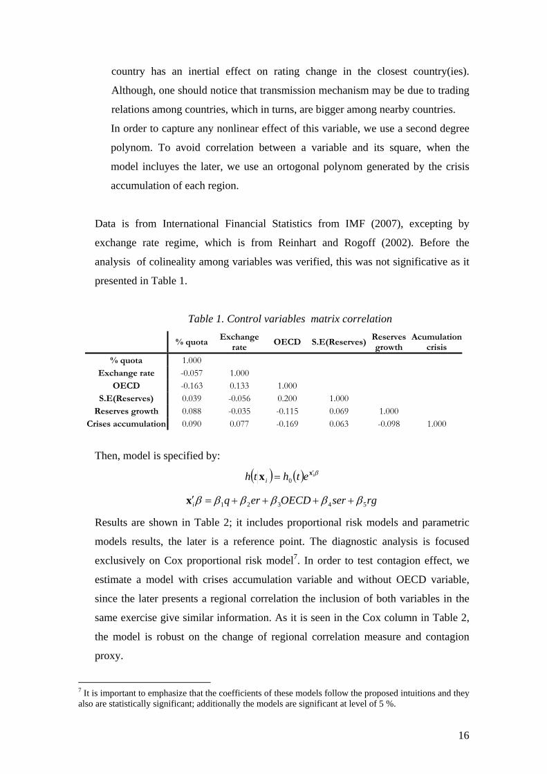
Data is from International Financial Statistics from IMF (2007), excepting by

exchange rate regime, which is from Reinhart and Rogoff (2002). Before the

analysis of colineality among variables was verified, this was not significative as it

presented in Table 1.

Table 1. Control variables matrix correlation

% quota Exchange

rate OECD S.E(Reserves)

Reserves growth

Acumulation crisis

% quota 1.000 Exchange rate -0.057 1.000

OECD -0.163 0.133 1.000 S.E(Reserves) 0.039 -0.056 0.200 1.000

Reserves growth 0.088 -0.035 -0.115 0.069 1.000 Crises accumulation 0.090 0.077 -0.169 0.063 -0.098 1.000

Then, model is specified by:

( ) ( ) βiethth ixx ′= 0

rgserOECDerqi 54321 ββββββ ++++=′x

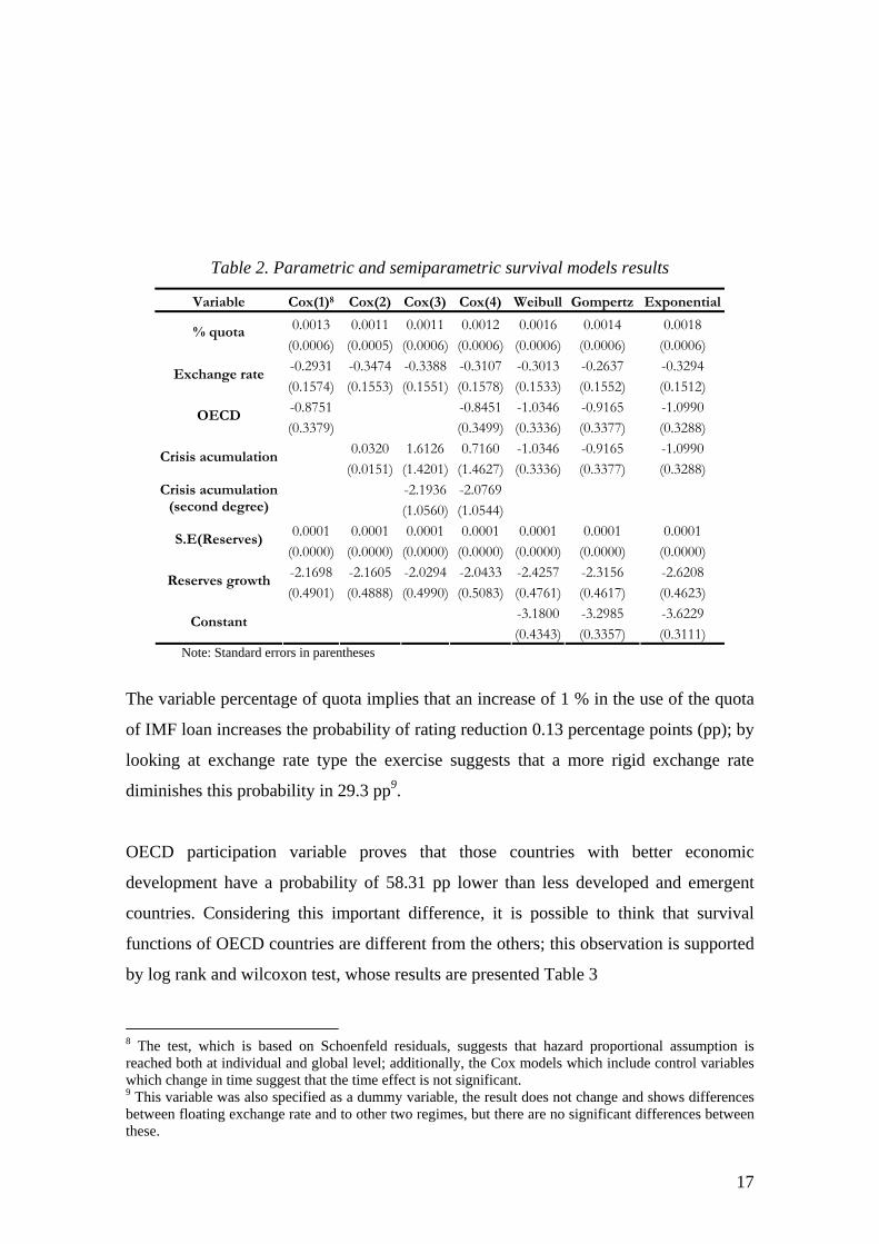
Results are shown in Table 2; it includes proportional risk models and parametric

models results, the later is a reference point. The diagnostic analysis is focused

exclusively on Cox proportional risk model7. In order to test contagion effect, we

estimate a model with crises accumulation variable and without OECD variable,

since the later presents a regional correlation the inclusion of both variables in the

same exercise give similar information. As it is seen in the Cox column in Table 2,

the model is robust on the change of regional correlation measure and contagion

proxy.

7 It is important to emphasize that the coefficients of these models follow the proposed intuitions and they also are statistically significant; additionally the models are significant at level of 5 %.

17

Table 2. Parametric and semiparametric survival models results

Variable Cox(1)8 Cox(2) Cox(3) Cox(4) Weibull Gompertz Exponential

0.0013 0.0011 0.0011 0.0012 0.0016 0.0014 0.0018 % quota (0.0006) (0.0005) (0.0006) (0.0006) (0.0006) (0.0006) (0.0006) -0.2931 -0.3474 -0.3388 -0.3107 -0.3013 -0.2637 -0.3294

Exchange rate (0.1574) (0.1553) (0.1551) (0.1578) (0.1533) (0.1552) (0.1512) -0.8751 -0.8451 -1.0346 -0.9165 -1.0990

OECD (0.3379) (0.3499) (0.3336) (0.3377) (0.3288)

0.0320 1.6126 0.7160 -1.0346 -0.9165 -1.0990 Crisis acumulation

(0.0151) (1.4201) (1.4627) (0.3336) (0.3377) (0.3288) -2.1936 -2.0769 Crisis acumulation

(second degree) (1.0560) (1.0544) 0.0001 0.0001 0.0001 0.0001 0.0001 0.0001 0.0001

S.E(Reserves) (0.0000) (0.0000) (0.0000) (0.0000) (0.0000) (0.0000) (0.0000) -2.1698 -2.1605 -2.0294 -2.0433 -2.4257 -2.3156 -2.6208

Reserves growth (0.4901) (0.4888) (0.4990) (0.5083) (0.4761) (0.4617) (0.4623)

-3.1800 -3.2985 -3.6229 Constant

(0.4343) (0.3357) (0.3111) Note: Standard errors in parentheses

The variable percentage of quota implies that an increase of 1 % in the use of the quota

of IMF loan increases the probability of rating reduction 0.13 percentage points (pp); by

looking at exchange rate type the exercise suggests that a more rigid exchange rate

diminishes this probability in 29.3 pp9.

OECD participation variable proves that those countries with better economic

development have a probability of 58.31 pp lower than less developed and emergent

countries. Considering this important difference, it is possible to think that survival

functions of OECD countries are different from the others; this observation is supported

by log rank and wilcoxon test, whose results are presented Table 3

8 The test, which is based on Schoenfeld residuals, suggests that hazard proportional assumption is reached both at individual and global level; additionally, the Cox models which include control variables which change in time suggest that the time effect is not significant. 9 This variable was also specified as a dummy variable, the result does not change and shows differences between floating exchange rate and to other two regimes, but there are no significant differences between these.

18

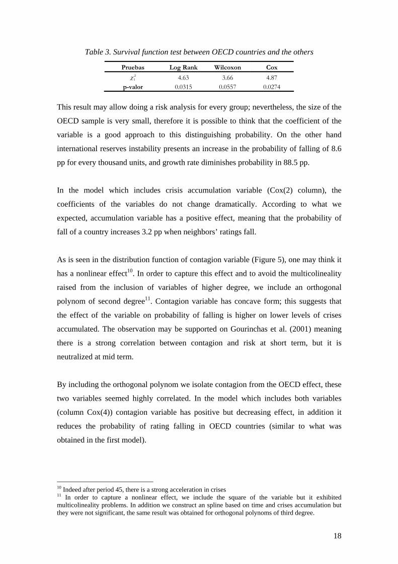
Table 3. Survival function test between OECD countries and the others

Pruebas Log Rank Wilcoxon Cox 21χ 4.63 3.66 4.87

p-valor 0.0315 0.0557 0.0274

This result may allow doing a risk analysis for every group; nevertheless, the size of the

OECD sample is very small, therefore it is possible to think that the coefficient of the

variable is a good approach to this distinguishing probability. On the other hand

international reserves instability presents an increase in the probability of falling of 8.6

pp for every thousand units, and growth rate diminishes probability in 88.5 pp.

In the model which includes crisis accumulation variable (Cox(2) column), the

coefficients of the variables do not change dramatically. According to what we

expected, accumulation variable has a positive effect, meaning that the probability of

fall of a country increases 3.2 pp when neighbors’ ratings fall.

As is seen in the distribution function of contagion variable (Figure 5), one may think it

has a nonlinear effect10. In order to capture this effect and to avoid the multicolineality

raised from the inclusion of variables of higher degree, we include an orthogonal

polynom of second degree11. Contagion variable has concave form; this suggests that

the effect of the variable on probability of falling is higher on lower levels of crises

accumulated. The observation may be supported on Gourinchas et al. (2001) meaning

there is a strong correlation between contagion and risk at short term, but it is

neutralized at mid term.

By including the orthogonal polynom we isolate contagion from the OECD effect, these

two variables seemed highly correlated. In the model which includes both variables

(column Cox(4)) contagion variable has positive but decreasing effect, in addition it

reduces the probability of rating falling in OECD countries (similar to what was

obtained in the first model).

10 Indeed after period 45, there is a strong acceleration in crises 11 In order to capture a nonlinear effect, we include the square of the variable but it exhibited multicolineality problems. In addition we construct an spline based on time and crises accumulation but they were not significant, the same result was obtained for orthogonal polynoms of third degree.

19

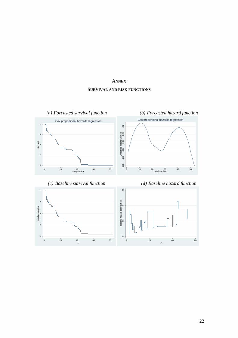
Survival, risk and cumulative risk functions getting out from Cox model, as well as

baseline estimations are in the Annex, where it is shown that the model replies the

regularities observed in the graphic analysis of the previous section which shows

financial falls persistence, which may be explained by replies in rating falling or region

contagion effects.

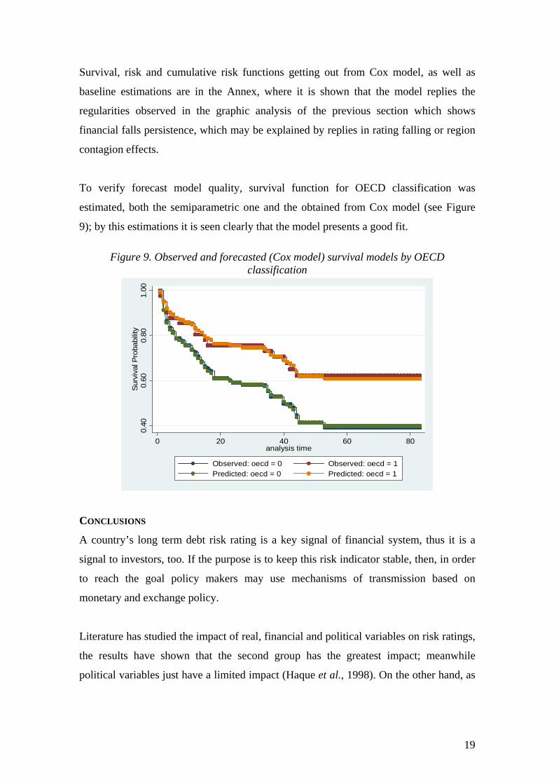
To verify forecast model quality, survival function for OECD classification was

estimated, both the semiparametric one and the obtained from Cox model (see Figure

9); by this estimations it is seen clearly that the model presents a good fit.

Figure 9. Observed and forecasted (Cox model) survival models by OECD classification

0.40

0.60

0.80

1.00

Surv

ival

Pro

babi

lity


Observed: oecd = 0 Observed: oecd = 1Predicted: oecd = 0 Predicted: oecd = 1

CONCLUSIONS

A country’s long term debt risk rating is a key signal of financial system, thus it is a

signal to investors, too. If the purpose is to keep this risk indicator stable, then, in order

to reach the goal policy makers may use mechanisms of transmission based on

monetary and exchange policy.

Literature has studied the impact of real, financial and political variables on risk ratings,

the results have shown that the second group has the greatest impact; meanwhile

political variables just have a limited impact (Haque et al., 1998). On the other hand, as

20

real variables are potentially endogenous with the rating, it is not possible to establish a

clear causality.

Because the space-temporal characteristic of survival models, it is feasible to combine

idiosyncratic country effects and time effects, which in turn is tied with financial

contagion. Therefore, in the studied period (1995-2001) which was characterized by a

great financial instability; through the model we conclude that an excessive

indebtedness with the IMF, exchange rigidities and international reserves instability

have a remarkable negative effect on risk ratings. On the other hand, by observing the

results between OECD and not OECD members and among regions, we found that the

higher is the GDP of a country the lower is the probability of rating fall, this event is

highly correlated with contagion effects by region which in turns has important positive

effect inside the model.

BIBLIOGRAPHY Bissoondoyal-Bheenick, Emawtee (2005) An analysis of the determinants of sovereign ratings. Global Finance Journal (15) 251– 280 Calvo, Sara and Carmen M. Reinhart (1996) Capital flows to Latin America: is there evidence of contagion effects. Policy research working paper 1619 Cleves, M., et al. (2004) An introduction to survival analysis using stata. Stata Press. Domaç, Ilker and Maria Soledad Martinez (2000) Banking Crises and Exchange Rate Regimes: Is There a Link? Policy Research Working Papers 2489 Eichengreen, Barry (1999) Toward a new international financial architecture. A practical Post-Asia Agenda. Institute for International Economics Gourinchas, Pierre-Olivier, Rodrigo Valdes and Oscar Landerretche (2001) Lending booms: Latin america and the World. NBER Working Paper #8249 International Monetary Fund (2007), International Financial Statistics. Database Haque, Nadeem U., Mark Nelson, and Donald J. Mathieson (1998) The Relative Importance of Political and Economic Variables in Creditworthiness Ratings IMF Working Paper 98/46 Jenkis, S. P., (1995). Easy Estimation Methods for Discrete-Time Duration Models. Oxford Bulletin of Economics and Statistics, 57, 129-138.

21

___________, (2005). Survival analysis. Institute for Social and Economic Research, University of Essex, Colchester. Kiefer, N. (1988). Economic Duration Data and Hazard Functions. Journal of Economic Literature, 26, 646-679. Krugman, Paul (1979) A model of Balance-of-Payments Crisis. Journal of Money, Credit and Banking 11:311-325 Loayza, Norman and Romain Ranciere (2005) Financial Development, Financial Fragility, and Growth. IMF Working Paper 170 Mackinnon, R. Huw, P. (1997) Credible Economic liberalization and overborrowing. American Economic Review Papers and Proceedings 87: 189-193 Manasse, Paolo, Nouriel Roubini, and Axel Schimmelpfennig (2003) Predicting Sovereign Debt Crisis IMF Working Paper, November 03/221 Obstfeld, Maurice (1997) Destabilizing effects of exchange rate escape clauses. Journal of International Economics 43:61-77 Ozkan, F. Gulcin and Alan Sutherland (1998) A currency crisis model with an optimizing policy maker. Journal of International Economics 44:339-364 Ratha, Dilip (2008) in http://dilipratha.com/countryrisk.htm in January 21st of 2008 Reinhart, C. (2002) Default, Currency Crisis and Sovereign Credit Ratings. NBER Working Paper 8738. Reinhart, C. (2001) Sovereign Credit Ratings Before and After Financial Crises in http://www.wam.umd.edu/~creinhar/Papers.html Reinhart, C. y Rogoff, K. (2002) The modern history of exchange rate arrangements: a reinterpretation. NBER Working Paper 8963.

22

ANNEX

SURVIVAL AND RISK FUNCTIONS

(a) Forcasted survival function (b) Forcasted hazard function

.6.7

.8.9

1S

urvi

val


Cox proportional hazards regression.0

05.0

06.0

07.0

08.0

09.0

1S

moo

thed

haz

ard

func

tion


Cox proportional hazards regression

(c) Baseline survival function (d) Baseline hazard function

.2.4

.6.8

1ba

selin

e su

rviv

or

0 20 40 60 80_t

0.0

5.1

.15

base

line

haza

rd c

ontri

butio

n

0 20 40 60_t

Country risk ratings and financial crises 1995 – 2001: a survival analysis

Documents