Contributions to Large-Signal Network Analysis Vrije Universiteit Brussel Faculteit Ingenieurswetenschappen Vakgroep ELEC Pleinlaan 2, B-1050 Brussels, Belgium Proefschrift ingediend tot het behalen van de academische graad van doctor in de ingenieurswetenschappen Frans Verbeyst Promotor: Prof. Dr. ir. Yves Rolain September 2006

Welcome message from author
This document is posted to help you gain knowledge. Please leave a comment to let me know what you think about it! Share it to your friends and learn new things together.
Transcript

Contributions toLarge-Signal Network Analysis
Vrije Universiteit BrusselFaculteit IngenieurswetenschappenVakgroep ELECPleinlaan 2, B-1050 Brussels, Belgium
Proefschrift ingediend tot het behalen van de academische graad vandoctor in de ingenieurswetenschappen
Frans Verbeyst
Promotor: Prof. Dr. ir. Yves Rolain
September 2006

Contributions toLarge-Signal Network Analysis
Vrije Universiteit BrusselFaculteit IngenieurswetenschappenVakgroep ELECPleinlaan 2, B-1050 Brussels, Belgium
Proefschrift ingediend tot het behalen van de academische graad vandoctor in de ingenieurswetenschappen
Frans Verbeyst
Voorzitter:Prof. Dr. ir. Jacques De Ruyck (Vrije Universiteit Brussel)
Vice-voorzitter:Prof. Dr. ir. Jean Vereecken (Vrije Universiteit Brussel)
Promotor: Prof. Dr. ir. Yves Rolain (Vrije Universiteit Brussel)
Secretaris:Prof. Dr. ir. Alain Barel (Vrije Universiteit Brussel)
Jury:Prof. Dr. ir. Don DeGroot (CCNi Measurement Services,
Andrews University, Michigan, USA)Prof. Dr. ir. Rik Pintelon (Vrije Universiteit Brussel)Prof. Dr. ir. Roger Pollard (University of Leeds, UK)Prof. Dr. ir. Johan Schoukens (Vrije Universiteit Brussel)Prof. Dr. ir. Steve Vanlanduit (Vrije Universiteit Brussel)

What lies behind us
and what lies in front of us
is nothing compared to
what lies within us.

Contributions to Large-Signal Network Analysis i
Preface
Acknowledgements
Abbreviations
CHAPTER 1: Software ArchitectureAbstract ................................................................................................ 1 - 2Introduction to object-oriented programming ....................................... 1 - 3Patterns for increased robustness ....................................................... 1 - 5
Handles and smart pointers ................................................................ 1 - 5Singletons ...................................................................................... 1 - 5
Patterns for increased flexibility ........................................................... 1 - 6Class and handle manager ................................................................. 1 - 6“Role” interface ................................................................................ 1 - 7Delegation versus inheritance ............................................................. 1 - 7Template Method pattern ................................................................... 1 - 8
Conclusion ........................................................................................... 1 - 9The open/close principle .................................................................... 1 - 9The Liskov substitution principle .......................................................... 1 - 9
References ........................................................................................ 1 - 10
CHAPTER 2: Enhancements to the nose-to-nose calibration technique.
Abstract ................................................................................................ 2 - 2Streamlined implementation ................................................................ 2 - 3Enhancement of the different parts ...................................................... 2 - 6
Time base drift estimation .................................................................. 2 - 6Positioning and width of time window ................................................... 2 - 8Enhanced time base distortion estimation and faster correction ............... 2 - 13Frequency domain interpolation using the chirp-z transform .................... 2 - 14
Conclusions ....................................................................................... 2 - 16References ........................................................................................ 2 - 17
CHAPTER 3: Comparison of the nose-to-nose and EOS-based calibration technique.
Abstract ................................................................................................ 3 - 2Amplitude comparison ......................................................................... 3 - 3
Table of contents

Table of contents
ii Contributions to Large-Signal Network Analysis
Overview ........................................................................................ 3 - 3Method #1: LSNA power measurement and scope in histogram mode ........ 3 - 4Method #2: LSNA power measurement and scope in normal mode ............ 3 - 5Method #3: amplitude characteristic based on nose-to-nose .................... 3 - 13Method #4: amplitude characteristic based on EOS ............................... 3 - 15Summary ...................................................................................... 3 - 17
Phase comparison ............................................................................. 3 - 18Conclusions ....................................................................................... 3 - 19References ........................................................................................ 3 - 20
CHAPTER 4: System identification approach applied to jitter estimation.
Abstract ................................................................................................ 4 - 2Modeling variance in the presence of additive and jitter noise ............ 4 - 3
Remark .......................................................................................... 4 - 5Estimators ............................................................................................ 4 - 6
Linear and nonlinear least squares ...................................................... 4 - 6Maximum Likelihood (ML) estimator ..................................................... 4 - 7Curiosity ....................................................................................... 4 - 10
Generation of simulation data ............................................................ 4 - 12Random number generator .............................................................. 4 - 15
Step 1: third order approximation of variance,known derivatives .............................................................................. 4 - 17
Estimated jitter standard deviation ..................................................... 4 - 17Estimated additive noise standard deviation ......................................... 4 - 18Value of the cost function ................................................................. 4 - 21Using the covariance matrix of the parameters ..................................... 4 - 24
Step 2: realistic variance,known derivatives .............................................................................. 4 - 27
Estimated jitter standard deviation ..................................................... 4 - 27Estimated additive noise standard deviation ......................................... 4 - 27Value of the cost function ................................................................. 4 - 27Using the covariance matrix of the parameters ..................................... 4 - 32
Step 3: realistic variance,derivatives based on sample mean ................................................... 4 - 36
Estimated jitter standard deviation ..................................................... 4 - 36Estimated additive noise standard deviation ......................................... 4 - 37Value of the cost function ................................................................. 4 - 39Using the covariance matrix of the parameters ..................................... 4 - 41
Step 4: influence of time base drift ..................................................... 4 - 44Time base jitter interpretable as time base drift ..................................... 4 - 48
Step 5: measurements ....................................................................... 4 - 50

Table of contents
Contributions to Large-Signal Network Analysis iii
Time base drift estimation ................................................................ 4 - 50Time base drift compensation ........................................................... 4 - 52Time base distortion estimation and compensation ................................ 4 - 54Time base jitter estimation ................................................................ 4 - 57The power of a solid stochastical framework ........................................ 4 - 61ML estimation ................................................................................ 4 - 62LS estimation ................................................................................ 4 - 63Bias in estimation of variance of additive noise ..................................... 4 - 64
Conclusions ....................................................................................... 4 - 66Future research ............................................................................. 4 - 66
References ........................................................................................ 4 - 67
CHAPTER 5: System identification approach applied to drift estimation.
Abstract ................................................................................................ 5 - 2Modelling and estimating drift in the presence of additive andjitter noise ............................................................................................ 5 - 3
Symbolic derivation .......................................................................... 5 - 5Analysis of the noise sources:additive white noise ............................................................................. 5 - 6
Is the noise circular complex distributed? .............................................. 5 - 6Weighted version of VLS .................................................................... 5 - 7Verification of the uncertainty on the estimated delays ............................. 5 - 7
Analysis of the noise sources:jitter noise .......................................................................................... 5 - 10
Simulation results ........................................................................... 5 - 10Calculation of the covariance matrix of the spectral noisein the frequency domain .................................................................. 5 - 18
The added value of the covariance matrixfor the WLS ........................................................................................ 5 - 25
LS parameter covariance matrix ........................................................ 5 - 25WLS estimator ............................................................................... 5 - 26
Simulations ........................................................................................ 5 - 27Estimators .................................................................................... 5 - 27Zero drift ...................................................................................... 5 - 27Linear drift .................................................................................... 5 - 28
Comparison to state-of-the-art methods ............................................ 5 - 30Comparison #1: no jitter, small additive noise ....................................... 5 - 33Comparison #2: no jitter, moderate additive noise ................................. 5 - 34Comparison #3: significant jitter, moderate additive noise ....................... 5 - 34Comparison #4: moderate jitter, small additive noise .............................. 5 - 35Comparison #5: moderate jitter, moderate additive noise ........................ 5 - 35Conclusions .................................................................................. 5 - 36

Table of contents
iv Contributions to Large-Signal Network Analysis
Measurements ................................................................................... 5 - 37Conclusions ....................................................................................... 5 - 41
Future research ............................................................................. 5 - 41References ........................................................................................ 5 - 42
CHAPTER 6: Volterra-based behavioural modelling.Abstract ................................................................................................ 6 - 2Introduction .......................................................................................... 6 - 3The one-tone VIOMAP and its inverse ................................................ 6 - 4Predistortion of narrowband signals based on an inverse VIOMAP .... 6 - 6One-tone and two-tone VIOMAP: some theory ................................... 6 - 7Measurement setup and results ........................................................ 6 - 10
Measurement setup ........................................................................ 6 - 10Model extraction. ............................................................................ 6 - 12Static two-tone VIOMAP and its inverse. ............................................. 6 - 15Predistortion based on static two-tone VIOMAP vs. one-tone VIOMAP. ...... 6 - 16
Conclusions ....................................................................................... 6 - 20References ........................................................................................ 6 - 21
Conclusions and ideas for further research
Publications
Patents
Awards

Contributions to Large-Signal Network Analysis v
Although scattering S-parameters have been around longer than I have, today, some
of us still manage to incompletely and therefore incorrectly define them as1 .
The other problem with S-parameters is that they got so ingrained that many peoplebelieve that they are omnipotent when it comes to solving microwave problems. Don’tget me wrong, S-parameter theory and the associated instrumentation has served andstill serves the RF community extremely well. Use it to its full power ... without denyingits basic assumptions: the superposition theorem, and therefore linear behaviour,must hold. S-parameters are all around, because they are technology-independent,because they can be measured and because they model the reflected and transmittedwaves as function of the incident waves and, as such, can be used during simulations.
Although its community is steadily growing, “Large-Signal Network Analysis” is still inits infancy and I guess not too many people can give a sufficiently correct descriptionof what LSNA stands for. Without claiming to hold the ultimate knowledge, LSNA hasthree major cornerstones. First, the device under test - referred to as the network - isput in (as) realistic (as possible) large-signal2 operating conditions, not only withrespect to input power levels, but also with respect to spectral content and mismatchconditions. Next, the behaviour of that DUT is completely and accuratelycharacterized in order to be analyzed. Because the basic quantities (voltage andcurrent) are measured, there is a natural link to make this data available in simulators.The data can be made available as is or through the use of a behavioural model.Finally, it is technology-independent, usable from the device up to the system level.It’s the engine of a unified approach ... “beyond S-parameters”. The behaviour of thedevice can be studied in the domain and in the format which is most convenient for theuser. Some people prefer the time domain, other the frequency domain. Some prefervoltage and current, others travelling voltage waves.
This work contains humble contributions to different aspects of “Large-Signal NetworkAnalysis”, which started more than 10 years ago.
Accurate measurements require both reliable hardware and software. I am the lastperson on earth to claim that building reliable hardware at microwave frequencies is apiece of cake. However, the hardware doesn’t have to be perfect. That’s becausethere are clever persons conceiving clever calibration algorithms. The software whichis used to control the hardware and to collect the raw data however must be perfect
1. corresponds to the transmitted or reflected voltage wave at port and represents the incident
voltage wave at port 2. large-signal refers to the fact that the stimulus becomes significant compared to the operating range
of the device
Sij
biaj----=
bi i aj
j
Preface

Preface
vi Contributions to Large-Signal Network Analysis
and must withstand the tooth of time. The chapter on “Software Architecture” shortlydescribes the basic principles used when designing and implementing the hardwareabstraction layer of a Large-Signal Network Analyzer.
Hardware at RF and microwave frequencies is never perfect. Fortunately, this can becompensated for, using a set of proper calibration elements and ditto calibrationtechniques. Calibration of a Large-Signal Network Analyzer is somewhat morecomplex than the calibration of a classical Vector Network Analyzer (VNA). On top of arelative calibration, the LSNA also requires an absolute power and phase calibration.The power calibration is performed using a power sensor, which is traceable up toNIST. The phase calibration however requires a new calibration element, which isreferred to as the Harmonic Phase Reference (HPR). The latter is a pulse generator,which itself must be calibrated. This is done using a high-frequency samplingoscilloscope. Unfortunately, this one isn’t perfect either and it seems to become anever-ending story. Luckily, the imperfections of the sampling oscilloscope can becompensated for using a “nose-to-nose” calibration technique. The basics, theindividual imperfections, their estimation and compensation are described in detail inanother PhD. In order to be really useful, additional work is required. The chapter“Enhancements to the nose-to-nose calibration technique” shortly describes thestreamlined implementation of the calibration technique and the replacement of someof the techniques by other techniques which were published and were proven to besuperior either in quality or in speed. I’m convinced that this additional work has beenessential in the adoption of the technique both by the people at NIST and by thecalibration lab of Agilent Technologies in Santa Rosa.
The nose-to-nose calibration and its application as a part of the calibration of theLarge-Signal Network Analyzer, fuelled the research at NIST related to their Electro-Optic Sampling (EOS) system. This system allows to characterize a photodiode up to110 GHz. By measuring the (known) impulse response of this photodiode using ahigh-frequency sampling oscilloscope, an alternative method does exist to determineboth the amplitude and the phase distortion introduced by this oscilloscope. Thediscrepancies that were reported by NIST are verified in the chapter “Comparison ofthe nose-to-nose and EOS-based calibration technique”. It is not the ambition of thechapter to find the reason of this discrepancy nor to eliminate it. Based on the workdescribed below, some of the required processing is performed in a different way, afterthe initial processing. As part of this additional verification, an exact expression isfound for the variance of different realizations of a sine wave in the presence ofnormally distributed jitter noise and additive noise. Implementations are realized bothin the absence and the presence of time base distortion.
The above verification has been the trigger for some recent research with respect tojitter estimation. Existing literature demonstrates that jitter, which has a symmetricalprobability density function, does not introduce any phase distortion. As such, jitterestimation was not given too much attention as a part of the nose-to-nose calibrationtechnique. Because jitter does have a low-pass effect on the amplitude, it becomesimportant when verifying the discrepancy that was reported for the amplitudecharacteristic. The main motivation for additional research is the observation that the

Preface
Contributions to Large-Signal Network Analysis vii
generally accepted first order model to describe the sample variance of repeatedmeasurements in the presence of both jitter noise and additive noise cannot explainsome of the measurement results that are obtained during the nose-to-nose and theEOS-based calibration. Backed up by the system identification knowledge, which isavailable at the department, the existing model is extended and different estimatorsare implemented. Several years earlier, I presented some of my behaviouralmodelling work based on neural networks to people of the department and I wasasked if the residual error was small or large. At that time, I didn’t understand therationale of that question and therefore I could not answer it. Fortunately, things havechanged and I feel the urge to ask that question too, each time others tell me how welltheir model works. Anyway, the power of a stochastical framework is demonstratedonce more when the excellent results that are obtained based on simulations are instrong contrast to the results based on measurements. It is found that the problem iscaused by overlooking the effect of time base drift compensation on the samplevariance. The solution that is found for that problem also properly deals with time basedistortion. The results are more than satisfactory. The rather extended “Systemidentification approach applied to jitter estimation“ chapter describes the work in detailand differs from the previous chapters by providing an avalanche of uncertaintyintervals.
During the review of the paper that describes the above research on jitter estimation,an enhanced version of the time base drift estimation has been proposed by one ofthe co-authors. This proposal and its implementation trigger new insights, especiallywhen jitter is present. Study of the covariance matrix of the spectral noise in thefrequency domain allows proper weighting of the contribution of the individual spectralcomponents to the cost function. This not only provides a relevant value for the costfunction, but it also reduces the uncertainty on the estimated drift in the presence of arealistic quantity of additive and jitter noise by a factor of 2. This work is described inthe “System identification approach applied to drift estimation“ chapter.
The last chapter reports on one of several contributions to another aspect of Large-Signal Network Analysis: closing the loop between measurements and simulations.Volterra-based behavioural modelling work has been performed in the early days. Theidea of predistorting a base-band signal using an inverse Volterra model is believed tobe original at that time and still today it seems to be alive and kicking. I vividlyremember that I was asked to write a C program to generate all unique combinationsof the spectral components at the inputs of a MIMO1 system, given the degrees ofnonlinearity of each output. The resulting model is referred to in literature asVIOMAP2. After performing some magic with pointers and recursion, I proudlypresented benchmarks for an increasing number of frequency components and anincreasing maximum degree of nonlinearity. History has taught me to be lessambitious. Nevertheless, original results are presented at the IMS 1995 conference3.
1. Multiple-Input-Multiple-Output.2. Volterra input-output map.3. IMS stands for International Microwave Symposium

Preface
viii Contributions to Large-Signal Network Analysis
A revised copy of the unpublished IMS paper can be found in the “Volterra-basedbehavioural modelling” chapter. It demonstrates that one must be very careful whenusing a model which is extracted using one class of excitation signals and then usedto predict the output of the system for another class of excitation signals.Unfortunately, there are still a lot of colleagues out there who need additionaleducation. The work also demonstrates that one should not overlook the effect of thebiasing circuitry. Other applications of the VIOMAP were targeted to bridge the gapbetween this Volterra-based technique and existing techniques. It is demonstratedthat the VIOMAP can be used as an alternative to load-pull measurements. TheVIOMAP is also a natural extension of S-parameters for weakly nonlinear devices.This statement is emphasized by extracting the VIOMAP for two different amplifiersand by predicting the behaviour of the cascade of both amplifiers by cascading theirindividual VIOMAPs.
Another application is the characterization at the fundamental frequency of thenonlinear behaviour of a device under test in a near 50 Ω environment. The combinedidea of linearizing the behavioural model with respect to the incident wave at theoutput and the use of readily available components like a load, open, short, adaptersand attenuators to synthesize different loads to extract such a model results in a USPatent Application Publication, No. US 2003/0057963 A1. This patent is filed asemployee of Agilent Technologies.
Recently, some new alternatives have been published to existing fundamental source-pull and load-pull techniques. Also, fundamental-only measurement-basedbehavioural models are introduced using either active injection in combination with amanual load tuner or using an electro-mechanical load tuner. This work has beenperformed as employee of NMDG Engineering and is referenced in the publication list.

Contributions to Large-Signal Network Analysis ix
When I graduated in 1986, I was sure about one thing: I would never get involved innonlinear stuff and especially not at microwave frequencies. At that time, both seemedmuch too complicated.
This PhD is yet another proof that there are no certainties in life. Fortunately, the latteris not one hundred percent true. As such, I first want to thank my wife Hilde forsupporting me in what I do and for the sacrifices, which seemed to converge to a localmaximum lately. It’s been a bumpy ride and it hasn’t been easy, but we made it !
Eli, thanks for being a great son, although there was much more mum than dad lately.This reminds me of being a son myself. I want to thank both my parents and myparents-in-law for giving me the opportunity to become what I am.
Next, I want to thank my promotor Yves Rolain, not only for his huge “open source”theoretical and practical knowledge, but also for his exceptional moral support. Thankyou for being there as a scientist and as a friend.
This PhD would never have been started nor finalized without the support of thedepartment ELEC. In particular, I want to thank Alain Barel, Rik Pintelon, JohanSchoukens and my promotor to provide the opportunity to “finally finalize” my PhD ona part-time basis at their department. I want to thank each of them for their enthusiasmduring the many discussions we had.
The same holds for Marc Vanden Bossche, who hired me as initial team member ofthe NMDG group of Hewlett - Packard and who allowed me to trade my full-time job atNMDG Engineering for a part-time job until “I was done”. I’m honoured to be part of hisnever-ending effort to make large-signal network analysis a success for each of us,meanwhile maintaining his attitude to live up to the spirit of Bill and Dave.
I had the privilege to work with several great people while I was with Hewlett - Packard(and later with Agilent Technologies). Doug Rytting was one of them and if there isone person, who is able to “promote” large-signal network analysis, it is surely him.
I want to say thanks to everyone at the department, including the technicians and thesecretaries, to my “room mates” Wendy and Salua, and to the new generation ofresearchers for their “energy” and for accepting an “older bloke”.
I want to thank all my co-authors too and all people worldwide whom I got in touchwith one way or another along the challenging large-signal network analysis road. Aspecial thanks to Tracy Clement at NIST for providing the measurement data that areused in the jitter and drift estimation chapters.
Acknowledgements

Acknowledgements
x Contributions to Large-Signal Network Analysis
Finally, I want to apologize to all other people who specifically contributed to this workand who are not explicitly mentioned here.
Merchtem, 06/06/2006

Contributions to Large-Signal Network Analysis xi
ADC A/D analog-to-digital (converter)
API application programming interface
ARFTG Automatic Radio Frequency Techniques Group
AWG arbitrary waveform generator
CLR common language runtime
CW continuous wave(form)
dB decibel
dBm decibels referenced to one milliwatt
DC direct current
DCA digital communication analyzer
DLL dynamic-link library
DUT device under test
EOS electro-optic sampling
FFT fast Fourier transform
GUI graphical user interface
HP Hewlett - Packard
HPR harmonic phase reference (see also REFGEN)
i.i.d. independent and identically distributed
IMS International Microwave Symposium
IMTC Instrumentation and Measurement Technology Conference
IQ in phase and quadrature phase
ISA industry standard architecture (bus)
Abbreviations

Abbreviations
xii Contributions to Large-Signal Network Analysis
IVI interchangeable virtual instrument
KIS keep it simple
LF low frequency
LOST load, open, short, thru
LS least squares
LSNA Large-Signal Network Analysis or Large-Signal Network Analyzer
MIMO multiple input multiple output
MLE ML maximum likelihood (estimator)
NIST National Institute of Standards and Technology
NMDG Network Measurement and Description Group
O/E opto-electrical (converter)
PC104 (ISA-based) personal computer (bus) utilizing 104 pins
PCI peripheral component interconnect (bus)
PDF probability density function
PISPO periodic in same period out
QAM quadrature amplitude modulation
REFGEN reference generator (see also HPR)
RF radio frequency
RMS root mean square
RTTI run-time type information
SNR S/N signal to noise (ratio)
SPMT single-pole multiple throw
TBDn time base distortion
var variance

Abbreviations
Contributions to Large-Signal Network Analysis xiii
VIOMAP Volterra input output map
VME versa module eurocard
VNA vector(ial) network analyzer
VXI VME extensions for instrumentation
WLS weighted least squares

Abbreviations
xiv Contributions to Large-Signal Network Analysis

Contributions to Large-Signal Network Analysis 1 - 1
• “Abstract” on page 1-2
• “Introduction to object-oriented programming” on page 1-3
• “Patterns for increased robustness” on page 1-5
• “Patterns for increased flexibility” on page 1-6
• “Conclusion” on page 1-9
• “References” on page 1-10
CHAPTER 1 Software Architecture

Software ArchitectureAbstract
1 - 2 Contributions to Large-Signal Network Analysis
Abstract
Characterization of the large-signal behaviour of a high-frequency active componentunder realistic conditions requires a measurement system, which is very versatile withrespect to both the applied excitations and mismatch conditions.
Given the disruptive character of such measurement systems, both the underlyinghardware and software must be kept as flexible as possible. A typical architecture of aLarge-Signal Network Analyzer (LSNA) is shown in figure 1-1.
The device under test is connected to the LSNA hardware. The hardware abstractionlayer allows the LSNA core software to communicate with this hardware in an abstractway. The design goal of this layer is to be able to replace part of the hardware by otherhardware with similar capabilities, without impacting the core software. The lattermainly takes care of the data collection and the calibration of the LSNA. Themeasured data is provided in different domains and formats and can be bothuncalibrated and calibrated. A user can interact with the system through a graphicaluser interface (GUI) and create applications running on top of the LSNA corefunctionality, using the LSNA application programming interface (API).
This chapter describes the hardware abstraction layer, which must be both robust, fastand flexible. Based on these requirements, this layer is written in C++. Furthermore,the necessary foundations are added to provide robustness and flexibility. The initialimplementation dates from the early 90’s, before similar idioms and patterns weredescribed in literature [1], [2]. Almost fifteen years later, the same software hassurvived the transition from VXI to both PC104 and PCI and provides the heartbeat ofthe MT4463 Large-Signal Network Analyzer, commercialized by Maury Microwavesand NMDG Engineering BVBA.
Figure 1-1. Typical architecture of a Large-Signal Network Analyzer.
Hardware Abstraction Layer
LSNA Core Functionality Layer
Data Representation &Application Layer
LSNA API
LSNA Hardware Layer
DUT
LSNA user
Hardware Abstraction Layer
LSNA Core Functionality Layer
Data Representation &Application Layer
LSNA API
LSNA Hardware Layer
DUTDUT
LSNA user LSNA user

Software ArchitectureIntroduction to object-oriented programming
Contributions to Large-Signal Network Analysis 1 - 3
Introduction to object-oriented programming
First, fundamental concepts of object-oriented programming, such as classes, objectsand abstraction are shortly introduced, based on an example: the LSNA test set.
The main functionality of an LSNA test set is to simplify its calibration by routing thesignal, which is applied to its input, to one of its outputs. Meanwhile other outputs areterminated, typically into 50 Ohms.
The set of possible test set modes is defined, as described in figure 1-2.
The name convention used for these modes answers the following simple question ina consistent way: “where is the calibration element connected?” or “what is theprimary calibration port?”.
LOST refers to the connection of a Load, Open, Short or Thru calibration element.PWM corresponds to the connection of a power sensor to allow absolute amplitudecalibration. REFGEN refers to the phase reference generator, which is in fact a pulsegenerator and used as part of the phase calibration of the LSNA.
A test set is able to indicate if it supports any of these modes, to put itself into thespecified mode and to return its actual mode. How this is done is of no concern to theusers of this test set. This in fact defines the abstract interface of a test set.
Figure 1-2. Example modes of a test set used as part of the Large-Signal Network Analyzer.
THRU
50 Ω
THRU
THRU
THRU
50 Ω
50 Ω
50 Ω
50 Ω
50 Ω
FORWARD AUX 2
REFGEN AUX 1
FORWARD PORT 1
REFGEN PORT 1
FORWARD PORT 2
REFGEN PORT 2
FORWARD AUX 1
REFGEN AUX 2
LOSTPWM
LOSTPWM
REFGEN
LOSTPWM
LOSTPWM
REFGEN
REFGEN
REFGEN
THRU
50 Ω
THRU
THRU
THRU
50 Ω
50 Ω
50 Ω
50 Ω
50 Ω
FORWARD AUX 2
REFGEN AUX 1
FORWARD PORT 1
REFGEN PORT 1
FORWARD PORT 2
REFGEN PORT 2
FORWARD AUX 1
REFGEN AUX 2
LOSTPWM
LOSTPWM
REFGEN
LOSTPWM
LOSTPWM
REFGEN
REFGEN
REFGEN

Software ArchitectureIntroduction to object-oriented programming
1 - 4 Contributions to Large-Signal Network Analysis
Classes describe the common characteristics and functionality of a group of similarobjects. Test sets can be realized using different hardware, typically using a set ofsingle-pole-multiple-throw (SPMT) switches and/or transfer switches. Each of theserealizations typically is given a model number and represents a concrete class.
Objects correspond to unique instantiations of a class. Each individual test set, itsuniqueness being represented by a unique serial number, corresponds to an object.
Software ArchitecturePatterns for increased robustness
Contributions to Large-Signal Network Analysis 1 - 5
Patterns for increased robustness
Handles and smart pointers
In the C and C++ programming language, the programmer is responsible for thedynamic memory management. The proper amount of memory must be allocated atruntime, when the object is constructed. When the object is no longer needed, theassociated dynamic memory must be freed. This must be done “just in time”.
If memory is released too soon, other objects may still hold a pointer to that memory.Such a pointer is referred to as a dangling pointer and results in undesired behaviourof the software and even system failure.
When the object is no longer needed and the programmer forgets to free thecorresponding memory, this memory cannot be reused later on. This situation isreferred to as memory leakage. Although memory is cheap these days and plenty of itis available, eventually the program will run out of memory and fail.
In order to avoid these problems and automate the release of memory, the C++ layerof the LSNA uses handles instead of pointers. Handles are objects which refer tosmart pointers. The latter keep track of how many times the underlying dynamicmemory is referenced. Because handles are objects, a programmer can rely on theC++ compiler and the correct implementation of the copy constructor, the assignmentoperator and the destructor of the Handle class. The required code is implementedonce, either as a macro or as a template. If this code is properly implemented, one isassured that the underlying dynamic memory is freed only if, and as soon as, no oneelse references this memory.
Finally, the handles should be implemented such that they allow late binding. Thelatter is a powerful mechanism to be used in combination with abstraction, i.e. theactual implementation of the abstract interface is determined at run-time instead of atcompile time.
Singletons
Sometimes it is important to make sure to have one and only one instance of a class.Typically this is the case for “manager” classes. The C++ layer of the LSNA uses twosuch classes, being the class manager and the handle manager. The former keepstrack of all LSNA-related classes being available to the software, the latter doing thesame for LSNA-related handles. It is essential for the robustness to make sure that allobjects communicate with “the” class manager and “the” handle manager. Accordingto [1], this is referred to as the Singleton pattern. The need for both a class and handlemanager as part of the LSNA C++ software is described in the next paragraph.

Software ArchitecturePatterns for increased flexibility
1 - 6 Contributions to Large-Signal Network Analysis
Patterns for increased flexibility
Given the disruptive nature of the Large-Signal Network Analyzer, both hardware andsoftware must be flexible. Over time the Large-Signal Network Analyzer has evolvedfrom a VXI-based instrument to a PC104-based instrument. The original calibrationmodule was replaced by a test set, while four one-channel VXI-based ADC cardswere replaced by one four-channel PCI-based ADC card.
Below, several patterns are shortly described, providing the required flexibility at thehardware abstraction level, such that the same core LSNA software can be used onall existing systems.
For the remainder of this chapter, a handle to an object will be referred to as either ahandle or an object.
Class and handle manager
Each software object, which is part of the LSNA, is referred to by a unique name. Ingeneral, each software object represents a hardware component. The functionality ofthese objects is implemented in classes and these too are referred to by a uniquename.
The mapping of unique object names onto unique handles is taken care of by thehandle manager. The same is done at the class level by the class manager.
All LSNA-related classes register themselves to the class manager. In the case ofstatic libraries this is done automatically by applying the appropriate pattern. In thecase of dynamic-link libraries (DLLs), one either needs to instantiate a dummy objectof each required type in the main function of the application or one can force thenecessary symbol references when linking the main application to the libraries.
Using names for both classes and objects, the actual hardware configuration can bestored in one or more configuration files. Each line of such a configuration file startswith the class name followed by the object name. At that moment both the class andhandle manager come into play. First the handle manager verifies if an object with thatname already exists. If this is the case and the object turns out to be of the correcttype, a handle to that object is returned by the handle manager.
If the object does not yet exist, the handle manager uses the class manager to createan object, based on the specified class name. In fact each LSNA-related classimplements two member functions which can be invoked by the class manager. Thefirst function allows the interactive configuration of the object, while the other readsthe remainder of the configuration of that object from file.

Software ArchitecturePatterns for increased flexibility
Contributions to Large-Signal Network Analysis 1 - 7
If the remainder of the configuration refers to other objects, the handle manager isused once more. When an object with the specified name already exists and if theobject turns out to be of the correct type, the handle manager returns a handle to thatobject. If the object does not yet exist and interactive configuration is allowed, a dialogis initiated with the user through the console window to configure the missing object.
Finally, a mechanism is implemented allowing to find out class information at run-time.This allows to verify if an object is an instantiation of a specified class or aninstantiation of a concrete subclass, in the case the specified class is an abstractclass. It also allows to find all concrete subclasses of a specified class. Again, this is apowerful feature when correctly used in combination with abstraction. After the initialimplementation as part of the LSNA, this mechanism was added to the C++ standardand is referred to as RTTI (Run-Time Type Information).
“Role” interface
Instrument drivers can be either very specific or rather abstract. Specific drivers havethe advantage that they allow to exploit the full power of the instrument, while abstractdrivers promote reusability and interchangeability. The hardware abstraction layer ofthe Large-Signal Network Analyzer contains both. However, only the abstract versionof the driver is made available to the outside world. This interface is based upon thefunctionality required by the Large-Signal Network Analyzer.
Recently, this concept is described as part of IVI (Interchangeable Virtual Instruments)[3] and more specifically as part of the Measurement and Stimulus SubsystemsSpecification. The latter describes the concept of a Role Control Module, which mapsan instrument interface on a “role” interface. This role interface corresponds to therequired functionality when the instrument or hardware is used as part of the Large-Signal Network Analyzer.
In [1] this concept is described as the Adapter pattern.
The IVI driver architecture also specifies different operational modes. One of them issimulation mode, which allows to write software based on the instrument driver beforethe physical instrument itself is available. This concept was used as part of thehardware abstraction layer way before it was published by the VXI Consortium.
Delegation versus inheritance
C++ promotes code reuse through inheritance. However, inheritance tends to beoverused, resulting in an explosion of the number of classes. An alternative toinheritance is delegation.
Proper combination of inheritance, delegation and abstraction is important whendealing with hardware which can be controlled in different ways. A good example is astep attenuator which can be controlled using either an Agilent E1339A Digital Output/

Software ArchitecturePatterns for increased flexibility
1 - 8 Contributions to Large-Signal Network Analysis
Relay Driver VXI interface card, an Agilent 11713A Attenuator/Switch Driver ordedicated PC104 hardware. It is necessary to separate the functionality of a stepattenuator from the way it is controlled.
Typical functionality of a step attenuator is to realize a specified attenuation asfaithfully as possible and to return the actually realized attenuation. In case the S-parameters are measured in a certain frequency range, the step attenuator can alsoreturn its S-parameter values for the actual attenuation as a function of frequency.This is a typical situation where subclassing is used: adding S-parameter capability tothe basic functionality of a step attenuator.
With respect to the control part of the step attenuator, first an abstract “role” interfaceis defined. Step attenuators are typically controlled by activating and deactivating oneor more sections. Each concrete implementation of this control API is written on top ofthe specific E1339A and 11713A driver and as such allows easy replacement of thecontrol hardware.
Finally a handle to this abstract “role” interface is defined as a part of the stepattenuator class, resulting in an orthogonal solution. The functionality of the stepattenuator itself can grow by proper subclassing. Meanwhile the control portion isdelegated through the handle. New control hardware can be added by properimplementation of the “role” interface.
Template Method pattern
Another pattern, which can be found in the hardware abstraction layer, is the TemplateMethod pattern.
This design pattern is mainly used to define the skeleton of a complex algorithm in thebase class and have the subclasses implement different versions for each part of thealgorithm.
The abstract step attenuator driver base class does not know how to activate ordeactivate a step attenuator section. However it keeps track of which section isactivated, such that the concrete subclasses are relieved from this burden. As suchthe abstract driver class defines a public activateSection () member function whichprovides the template. This template correctly keeps track of the activated sectionsand leaves the physical activation or deactivation to the concrete subclass by callingthe appropriate private virtual doActivateSection () member function. Defining amember function as private, makes sure that this function cannot be invoked fromoutside the abstract base class. Virtual functions are used in C++ to support the latebinding, as explained on page 1-5.

Software ArchitectureConclusion
Contributions to Large-Signal Network Analysis 1 - 9
Conclusion
We conclude with two well-known principles [4] in the object-oriented design world,which help to create more scalable, robust and reusable applications.
The open/close principle
Bertrand Meyer stated in 1996 that: “Software entities (classes, modules, etc.) shouldbe open for extension, but closed for modification.”
In plain English this means that software modules should be designed such that theirbehaviour can be modified (open) without making source code modifications (closed),but by adding new code.
The Liskov substitution principle
Barbara Liskov stated 8 years earlier that: “Derived classes must be usable throughthe base class interface without the need for the user to know the difference.”
Both principles emphasis the proper usage of abstraction. Given the fact that theLSNA hardware abstraction layer software was conceived in the early nineties and issuccessfully used today in both legacy (VXI-based) and new (PC104/PCI-based)LSNA systems, without causing any frustration to both conceiver and users, it can beclaimed that the used approach “simply works”.

Software ArchitectureReferences
1 - 10 Contributions to Large-Signal Network Analysis
References
[1] E. Gamma, R. Helm, R. Johnson, J. Vlissides, “Design Patterns. Elements ofReusable Object-Oriented Software,” Addison-Wesley, 1995.[2] D. Box, “Essential COM,” Addison-Wesley, 1997.[3] “IVI-3.10: Measurement and Stimulus Subsystem (IVI-MSS) Specification,” 2001,http://www.ivifoundation.org.[4] R. Martin, “Agile Software Development Principles, Patterns, and Practices,” Pren-tice Hall, 2002.

Contributions to Large-Signal Network Analysis 2 - 1
• “Abstract” on page 2-2
• “Streamlined implementation” on page 2-3
• “Enhancement of the different parts” on page 2-6
• “Conclusions” on page 2-16
• “References” on page 2-17
CHAPTER 2 Enhancements to the nose-to-nose calibration technique.
Enhancements to the nose-to-nose calibration technique.Abstract
2 - 2 Contributions to Large-Signal Network Analysis
Abstract
A Large-Signal Network Analyzer is conceived to analyze the behaviour of nonlineardevices. This implies that the superposition principle no longer holds for thesedevices. Even when applying a pure sine wave at the input of such a device andterminating it into 50 Ohm, the reflected and transmitted voltage wave will no longerbe a pure sine wave. As such, in order to accurately measure incident and scatteredvoltage waves, not only a relative calibration like Short - Open - Load - Thru isrequired, but also a power and phase calibration. The power calibration is performedusing a calibrated power sensor, while phase calibration is performed using acalibrated harmonic phase reference. The latter is a pulse generator which has asufficiently rich harmonic content for a sufficiently broad range of fundamentalfrequencies. In order to use this pulse generator as an additional calibration standard,one needs to know the exact phase relationship between the different spectralcomponents of the pulse at each fundamental frequency1.
Therefore the harmonic phase reference is measured using a high-frequencysampling oscilloscope. Unfortunately this sampling oscilloscope also introducesdistortions. These are mainly caused by the non-ideal time base and the non-idealimpulse response of the sampling oscilloscope, resulting in both amplitude and phasedistortion. Nonlinear distortions are avoided by limiting the amplitude of the measuredsignals, while offset and gain errors are removed by performing a vertical calibration.
The list of distortions introduced by a high-frequency sampling oscilloscope were firststudied and described separately in [1]. The characterization and compensation ofthese distortions are referred to as the “nose-to-nose” calibration technique. In orderto be really useful, the problems and solutions described in [1] needed additionaleffort. The first contribution to the enhancement of the nose-to-nose calibrationtechnique is the implementation of a streamlined process, such that the calibrationcan be performed in a repetitive way and, if necessary, by a technician. Furthermore,it allowed to share this procedure in detail with people from NIST for thoroughcrossverification. As a result, numerous articles were published by NIST related to the“nose-to-nose” calibration technique [2]-[7]. Finally, the procedure was transferred intothe calibration lab of Agilent Technologies at Santa Rosa in order to allow the phasecalibration of the Agilent 86030A 50 GHz Lightwave Component Analyzer, which gaveit a unique competitive advantage and contributed significantly to its success. Thesecond contribution is the replacement of techniques described in [1] by othertechniques, which are superior either in quality or in speed.
Starting from a nose-to-nose calibrated oscilloscope, one can characterize either theharmonic phase reference to be used as part of the Large-Signal Network Analyzer orthe opto-electrical subsystem of the Lightwave Component Analyzer.
1. This fundamental frequency corresponds to the repetition frequency of the pulse.

Enhancements to the nose-to-nose calibration technique.Streamlined implementation
Contributions to Large-Signal Network Analysis 2 - 3
Streamlined implementation
In order to be able to perform nose-to-nose calibrations on a regular basis and inorder to allow a trained technician to perform these calibrations, a streamlinedprocess is implemented in VEEtest™ from Agilent Technologies. The full calibrationprocess typically takes 4 hours.
First, a time base distortion measurement of the scope is performed. This requires themeasurement of sine waves at two or more non-harmonically related frequencies. Ateach frequency, the sine wave must be measured twice, where ideally the secondmeasurement has a phase shift of 90° with respect to the first measurement. Typically,this is taken care of by using two channels and adding a delay line in the secondchannel, resulting in a phase shift of approximately 90° at discrete frequencies. Theusage of different frequencies allows the estimation method [8] to discriminatebetween a harmonic due to nonlinear behaviour and due to time base distortion. Thedetection of the time base distortion is insensitive when the slope of the applied signalis small. Using a sine wave, the slope is minimal in the extrema and maximal in thezero crossings. Applying a 90° phase shift, the delayed sine wave has a maximalslope whenever the original sine wave has a minimal slope and vice versa. Oncethese measurements are performed, an estimate for the time base distortion and itsuncertainty is obtained. Figure 2-1 shows the estimated time base distortion, definedas , the non-equidistant time stamps being represented by ;
corresponds to the time sample index and represents the assumed constant
equivalent-time sample rate. For an ideal time base, all values equal zero.
Acquiring 128 dual-channel traces of 2048 points at 12.4, 13.6 and 14.8 GHz, using
Figure 2-1. Estimated time base distortion as part of the nose-to-nose calibration.
TBDn i[ ] ti i ∆t⋅–= tii ∆t
TBDn i[ ]
64 65 66 67time ns
4
2
2
estimatedTBDn ps

Enhancements to the nose-to-nose calibration technique.Streamlined implementation
2 - 4 Contributions to Large-Signal Network Analysis
[8], the 95% confidence interval on the estimated time base distortion is approximately0.075 ps.
Next, the combined impulse response of two sampling oscilloscopes is measuredusing a “nose-to-nose” setup (figure 2-2). To do so, the inputs of two samplingoscilloscopes are connected to each other. A DC offset is applied to one oscilloscope.Whenever its samplers are closed, a pulse is fired from the internal samplers towardsthe input connector of the oscilloscope. This pulse is referred to as the kickout pulse.The nose-to-nose calibration technique is based on the assumption that the kickoutpulse is proportional to the impulse response of the sampling oscilloscope and isdescribed in detail in [1]. This kickout is then measured by the second samplingoscilloscope. The measured pulse is the convolution of the impulse response of bothoscilloscopes. By measuring 3 sampling oscilloscope combinations, it is possible toretrieve the impulse response of each contributing sampling oscilloscope (Eq. 2-1).These combinations are referred to as Mij measurements, where i represents thekickout-receiving oscilloscope and j represents the kickout-generating oscilloscope.
Eq. 2-1
In order to estimate and reduce the uncertainty on each Mij measurement, properaveraging is required. Since it is possible that the time base drifts, this phenomenonmust be estimated and compensated before averaging. The drift is mainly caused bytemperature variations in combination with air flow. During this step of the procedure,the time base drift is estimated and compensated before averaging. Also, based onthe mean value and the variance of the pulse in the time domain, an estimate is givenfor the jitter standard deviation. More recent work on jitter estimation is described in aseparate chapter: “System identification approach applied to jitter estimation”.
A portion of the strobe pulse, which fires the samplers, leaks through towards theoutput (the input connector). In order to eliminate this common mode portion of thekickout, two measurements are performed. First a positive DC offset and then anegative DC offset is applied to the kickout-generating sampling oscilloscope. The
Figure 2-2. The “nose-to-nose” setup.
±100 mV
±∆
offset
sampling scope B
M21 ÷ H2 . H1
H2 50 psH1
sampling scope A
±∆plug-in 1 plug-in 2
±100 mV
±∆
offset
sampling scope B
M21 ÷ H2 . H1
H2 50 psH1
sampling scope A
±∆plug-in 1 plug-in 2
M12 H1 H2⋅÷M13 H1 H3⋅÷
M12 M13⋅M23
------------------------- H1÷
M23 H2 H3⋅÷

Enhancements to the nose-to-nose calibration technique.Streamlined implementation
Contributions to Large-Signal Network Analysis 2 - 5
inversion of polarity will cause a polarity reverse for the kickout pulse, while it willleave the strobe contribution untouched. Hence, after averaging both the positive andnegative kickout and after proper alignment, one can subtract both kickouts to removethe common mode contribution of the strobe pulse.
After these three Mij measurements, a second time base distortion measurement isperformed to verify if the time base distortion has not changed during these Mijmeasurements.
Finally, postprocessing is performed to correct the Mij data, based on the estimatedtime base distortion [9]. In order to provide the amplitude and phase distortion of thesampling oscilloscope on a specified frequency grid, a chirp-z transform [10] isapplied. Using a proper combination of the corrected and interpolated Mij data, bytaking the mismatch of each oscilloscope and the required adapter into account andafter correcting for the low-pass effect of the jitter on the amplitude characteristic, oneends up with an estimate of the amplitude and phase characteristic of the threeoscilloscope plug-ins separately.
This procedure and its implementation was shared with - and explained to - peoplefrom the Optoelectronics Division, the Statistical Engineering Division and the Radio-Frequency Technology Division within NIST. The procedure was re-implementedindependently at NIST. No anomalies were found and the above procedure wasdescribed in detail [2].

Enhancements to the nose-to-nose calibration technique.Enhancement of the different parts
2 - 6 Contributions to Large-Signal Network Analysis
Enhancement of the different parts
The implementation was performed using an Agilent 83480 Digital CommunicationsAnalyzer (DCA) and three dual-channel 50 GHz 83484A plug-ins. Later, the code wasadapted to support also the Agilent 86100 DCA Oscilloscope. Both instruments useequivalent-time sampling.
Time base drift estimation
The best way to get rid of the time base drift is not to have it at all. Hence, one shouldalways try to minimize sudden temperature variations and uncontrolled air flow whenperforming measurements using a high-frequency sampling oscilloscope.
The logarithmic averaging of the spectral data proposed and described in [1] has thedisadvantage that a bias on the amplitude estimation is introduced which becomessignificant when the S/N ratio approximates 0 dB1. Also, logarithmic averaging doesnot decrease the noise floor. This turned out to be a limitation during the measurementof the impulse response of the opto-electrical subsystem of the Lightwave ComponentAnalyzer, given its very poor S/N ratio (< 0 dB). As such, it was decided to replace thelogarithmic averaging by regular averaging after estimating and compensating for thetime drift.
The time base drift is estimated by minimizing
Eq. 2-2
with respect to , within the bandwidth2 of the signal. represents the
measured spectral data of the reference signal at , while
represents the corresponding measured spectral data of the signal to be aligned with
respect to the reference signal. , where represents the
width of the time window, used to capture the impulse response. A starting value for is obtained, either based on a crosscorrelation test or by calculating the value of thecost function for a limited range of values on a sufficiently dense grid.
1. Based on equation (3.6-6) of [1] the bias on the amplitude estimation for a S/N ratio of 0 dB equals 0.9 dB.
2. In the case of impulse responses, measured using the 50 GHz sampling oscilloscopes, frequencies up to the first transmission zero (70 GHz) of the sampling oscilloscope are taken into account.
V Xref ωm( ) ejωmτ–
X ωm( )⋅–2
m 1=
M
=
τ Xref ωm( )
ωm 2πfm= X ωm( )
ωm m ω0⋅ m 2πT0------⋅= = T0
τ
τ

Enhancements to the nose-to-nose calibration technique.Enhancement of the different parts
Contributions to Large-Signal Network Analysis 2 - 7
In the actual implementation, the first measurement is taken as a reference and allsuccessive measurements are aligned with respect to that reference. In [6], it is shownthat a better alignment is possible when estimating the relative shifts of eachmeasurement with respect to all other measurements or by using an adaptivereference. Because these methods require that one keeps track of all the realizations,these methods are not implemented as part of the streamlined implementation.Furthermore, a comparison of the estimated drifts under realistic conditions (figure 2-3, figure 2-4), shows a good correspondence between the actual implementation andthe optimal implementation referred to in [6]. Furthermore, in the “System identificationapproach applied to jitter estimation” chapter, it is explained that time base jitter isinterpreted as time base drift and smoothing of the estimated time base drift isproposed.
Due to the presence of the feedthrough of the strobe pulse, one must measure apositive and negative kickout to eliminate this unwanted response. To minimize theelapsed time between the measurement of a positive and a negative kickout, themeasurement of a positive kickout is followed immediately by the measurement of anegative kickout. Using the above method, all positive kickouts can be aligned andaveraged. The same is done for the negative kickouts.
Finally the mean value of the positive kickout and the mean value of the negative
pulse must be aligned with respect to each other before they can be subtracted. Let
be the estimated time base drift of the th measurement of the positive kickout
with respect to the first measurement, while is the equivalent for the negative
kickout. It is observed that the overall shape of closely resembles that of as
Figure 2-3. Estimated time base drift (x: actual implementation, dots: implementation proposed by NIST [6]) based on 500 impulse response measurements performed at NIST.
100 200 300 400 500index
0.5
1
1.5
2
est. drift ps
τk+ k
τk-
τk- τk
+
Enhancements to the nose-to-nose calibration technique.Enhancement of the different parts
2 - 8 Contributions to Large-Signal Network Analysis
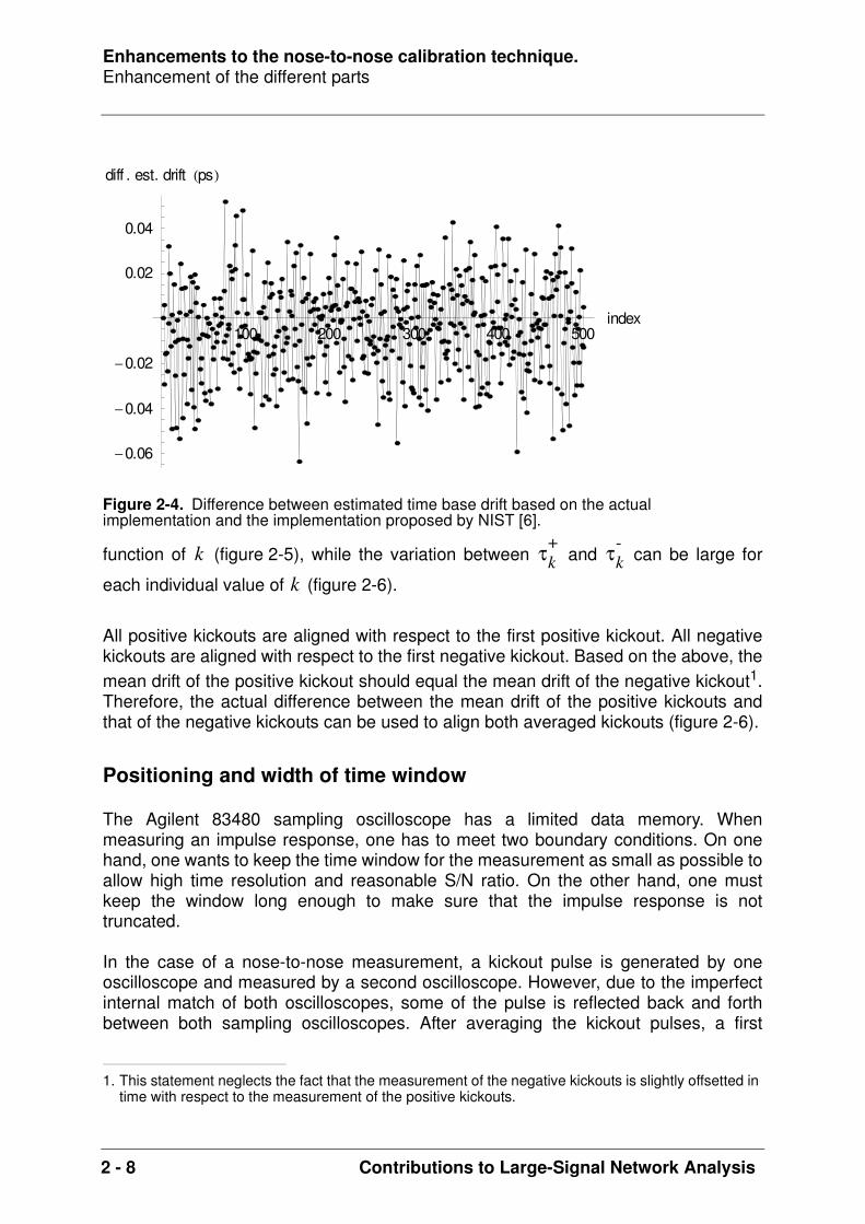
function of (figure 2-5), while the variation between and can be large for
each individual value of (figure 2-6).
All positive kickouts are aligned with respect to the first positive kickout. All negativekickouts are aligned with respect to the first negative kickout. Based on the above, themean drift of the positive kickout should equal the mean drift of the negative kickout1.Therefore, the actual difference between the mean drift of the positive kickouts andthat of the negative kickouts can be used to align both averaged kickouts (figure 2-6).
Positioning and width of time window
The Agilent 83480 sampling oscilloscope has a limited data memory. Whenmeasuring an impulse response, one has to meet two boundary conditions. On onehand, one wants to keep the time window for the measurement as small as possible toallow high time resolution and reasonable S/N ratio. On the other hand, one mustkeep the window long enough to make sure that the impulse response is nottruncated.
In the case of a nose-to-nose measurement, a kickout pulse is generated by oneoscilloscope and measured by a second oscilloscope. However, due to the imperfectinternal match of both oscilloscopes, some of the pulse is reflected back and forthbetween both sampling oscilloscopes. After averaging the kickout pulses, a first
Figure 2-4. Difference between estimated time base drift based on the actual implementation and the implementation proposed by NIST [6].
1. This statement neglects the fact that the measurement of the negative kickouts is slightly offsetted in time with respect to the measurement of the positive kickouts.
100 200 300 400 500index
0.06
0.04
0.02
0.02
0.04
diff . est. drift ps
k τk+ τk
-
k
Enhancements to the nose-to-nose calibration technique.Enhancement of the different parts
Contributions to Large-Signal Network Analysis 2 - 9
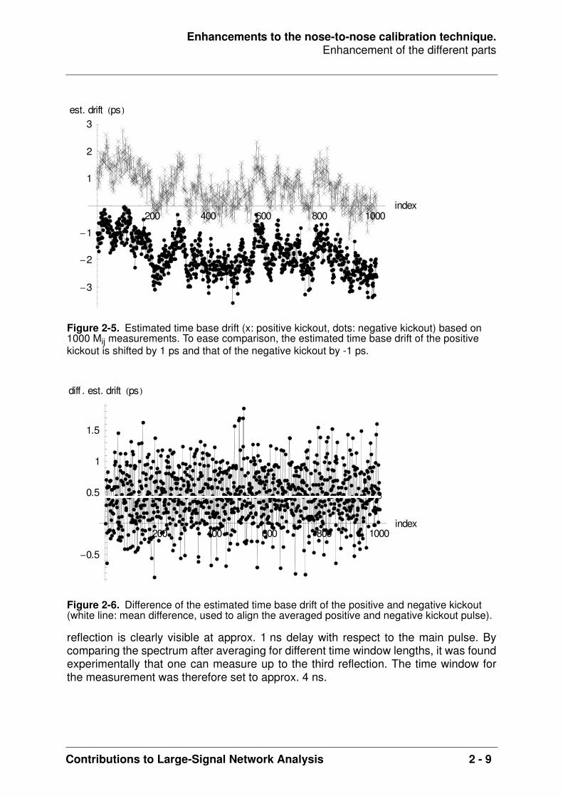
reflection is clearly visible at approx. 1 ns delay with respect to the main pulse. Bycomparing the spectrum after averaging for different time window lengths, it was foundexperimentally that one can measure up to the third reflection. The time window forthe measurement was therefore set to approx. 4 ns.
Figure 2-5. Estimated time base drift (x: positive kickout, dots: negative kickout) based on 1000 Mij measurements. To ease comparison, the estimated time base drift of the positive kickout is shifted by 1 ps and that of the negative kickout by -1 ps.
Figure 2-6. Difference of the estimated time base drift of the positive and negative kickout (white line: mean difference, used to align the averaged positive and negative kickout pulse).
200 400 600 800 1000index
3
2
1
1
2
3est. drift ps
200 400 600 800 1000index
0.5
0.5
1
1.5
diff . est. drift ps

Enhancements to the nose-to-nose calibration technique.Enhancement of the different parts
2 - 10 Contributions to Large-Signal Network Analysis
It was found that the actual distortion of certain portions of the time base of the50 GHz sampling oscilloscopes varies both with the trigger frequency and theselected time step. This means that the time base distortion measurement must beperformed using the same trigger and time step settings as the ones that are usedduring the actual measurement. Due to practical limitations of the samplingoscilloscope, the trigger frequency during nose-to-nose can not be increased above2.5 kHz. Due to other trigger hardware limitations, the smallest achievable triggerfrequency during the measurement of the time base distortion is approx. 5 kHz. It wasfound experimentally that the impacted regions of the time base are located at thebeginning of the time window and after each discontinuity of the time base. For theAgilent 83480A Digital Communication Analyzer, the position of these discontinuitiesis known to be located at 22 ns + k.4 ns, . The discontinuity of the time base isdue to the usage of a 250 MHz restartable oscillator in combination with a fine ramp of4 ns to create the time base. The impacted regions were found to span up to severaltenths of nanoseconds and the spans seem to increase with temperature. Figure 2-7up to figure 2-10 show the impact of changing the trigger repetition rate on the timebase distortion.
As such, it is important that the main pulse and its main reflections are not located inthis region. Therefore the time window is set to start at 63 ns (1 ns after the 62 nsdiscontinuity) and the main pulse is located at 0.5 ns delay with respect to the leftedge of the time window.
The shape of the difference of the estimated time base distortion (figure 2-10)deserves some additional attention. Because of the equivalent-time sampling, thephysical time between two successive sampling instants does not correspond to the
Figure 2-7. Estimated time base distortion (trigger rep. rate of 4.7 kHz and 27 kHz). To ease comparison, the estimated time base distortion using the 4.7 kHz trigger is shifted by 1 ps (upper curve) and that of the 27 kHz trigger is shifted by -1 ps (lower curve).
k N∈
64 65 66 67time ns
4
2
2
4
est. TBDn ps

Enhancements to the nose-to-nose calibration technique.Enhancement of the different parts
Contributions to Large-Signal Network Analysis 2 - 11
specified time step, but is determined by the trigger period1. As such, using a triggerrepetition rate of 27 kHz and using an equivalent-time step of 1 ps, a time window of0.17 ns corresponds to 170 samples and a physical time of 6.3 ms. Using a triggerrepetition rate of 4.7 kHz, the same physical time of 6.3 ms corresponds to
Figure 2-8. Difference of estimated time base distortion (trigger rep. rate of 4.7 kHz versus 27 kHz).
Figure 2-9. Difference of estimated time base distortion (trigger rep. rate of 4.7 kHz versus 27 kHz). Zooming in to the start of the window.
1. For the 83480 DCA, the internal sample frequency equals the trigger repetition rate, if this one is smaller than or equal to 40 kHz. Otherwise the internal sample frequency is limited to 40 kHz.
64 65 66 67time ns
1.5
1
0.5
0.5
1
1.5
2
diff .est. TBDn ps
63.05 63.1 63.15 63.2 63.25 63.3 63.35time ns
2
1.5
1
0.5
0.5diff . est. TBDn ps

Enhancements to the nose-to-nose calibration technique.Enhancement of the different parts
2 - 12 Contributions to Large-Signal Network Analysis
30 samples and an equivalent-time of 0.03 ns. This means that a phenomenon with agiven physical duration will manifest itself differently, depending on the applied triggerrepetition rate. Figure 2-11 shows a time base distortion step of 2.2 ps, which linearlydecreases as function of the physical time. As explained above, the impactedequivalent-time is different for a trigger repetition rate of 27 kHz and 4.7 kHz.Subtracting this effect results in a difference which is very similar to the one shown infigure 2-10.
Figure 2-10. Difference of estimated time base distortion (trigger rep. rate of 4.7 kHz versus 27 kHz). Zooming in to the portion of the time base at the discontinuity of 66 ns.
Figure 2-11. Simple model for the difference of the estimated time base distortion, corresponding to different trigger repetition rates. (long dashed line: 4.7 kHz trigger, short dashed line: 27 kHz trigger, thick line: difference of short and long dashed line).
65.9 65.95 66.05 66.1 66.15 66.2 66.25 66.3time ns
0.5
0.5
1
1.5
2diff . est. TBDn ps
65.9 65.95 66.05 66.1 66.15 66.2 66.25 66.3time ns
0.5
0.5
1
1.5
2
2.5diff . est. TBDn ps
Enhancements to the nose-to-nose calibration technique.Enhancement of the different parts
Contributions to Large-Signal Network Analysis 2 - 13
Enhanced time base distortion estimation and faster correction
The original time base distortion estimation is replaced by a better technique, whilethe compensation is replaced by a faster technique. The latter allows to choose asimple local interpolator such that the systematic interpolation error remains below thenoise floor of the reconstructed signal.
The original time base distortion estimation, as described in [1], basically performs aphase demodulation to extract the time base distortion. Systematic errors areintroduced because of two reasons. First, the method assumes that the time basedistortion can be represented by a band limited signal. This explains the modellingerrors around the discontinuities of the time base. Also, the windowing which isperformed in the time domain to reduce leakage, introduces large systematic errors atthe boundaries of the time window.
The estimation is replaced by the maximum likelihood estimator (MLE), described in[8]. It combines the advantages of a non-parametric time base and the efficiency androbustness provided by the use of a statistical framework. In practice, the comparisonof the actual value of the cost function and its expected value allows to verify for thepresence of model errors. For instance, the method requires measurements at two ormore non-harmonically related frequencies to distinguish between harmonics due totime base distortion and due to the (vertical) nonlinear behaviour of the oscilloscope.Harmonics can also be produced by the source. It was found that using certaincombinations of frequencies, the actual cost was significantly larger than the expectedone. It turned out that this was caused by the fact that the actual time base distortionvaried with the applied frequency, while the method assumes that the time basedistortion is independent of the applied frequency. The second advantage of thestatistical framework is that uncertainty bounds are provided, which can be used toprovide uncertainty bounds for the overall nose-to-nose method.
Once the time base distortion has been estimated, the next step is to compensate theMij measurements for this distortion. Although this may seem to be simple, the originaltime base distortion compensation, as described in [1], is very time consuming. Thecompensation is based on the construction of a least-squares estimator and requiresthe solution of a set of linear equations in a least-square sense. is a
real matrix, represents the assumed number of spectral
components and corresponds to the number of non-equidistant measured time
points. A typical value for is 2048 while is approx. 300 to 600. Using singular
value decomposition1 to calculate the solution, it was found that the calculation is too
time consuming. Indeed, a typical solver requires operations tosolve this set of equations. As such, it does not allow a Monte Carlo analysis to study
1. based on the implementation in C++ of a commercially available mathematical library M++.
y A x⋅= AN 2C 1+( )× C
NN C
O N2
2C 1+( )⋅( )

Enhancements to the nose-to-nose calibration technique.Enhancement of the different parts
2 - 14 Contributions to Large-Signal Network Analysis
the uncertainty after time base distortion correction, taking both the uncertainty on theestimated time base distortion and the uncertainty on the sample values into account.
To speed up the compensation, the solution of the set of equations is replaced by aKIS (“Keep It Simple”) approach as described in [9]. The cubic interpolation method isvery fast and requires only operations. The error introduced by this
interpolation increases with the relative bandwidth1 of the signal to be interpolated.Fortunately, based on the inherent high oversampling rate of an equivalent-timesampling oscilloscope, the bandwidth of the measured signal relative to the samplingfrequency is low: given a signal bandwidth of approx. 50 GHz, a 4 ns time window and2000 points, the relative bandwidth is 0.1. In worst case, the systematic deviation fromthe equidistant time grid2 equals : the sampling instance based on the distortedtime base is located right in between the ideal equidistant sampling instances. For thisrelative bandwidth and systematic deviation, based on the simulations performed in[9], the mean squared error is approx. -40 dB relative to the root-mean-square (RMS)value of the signal.
A typical value for the jitter standard deviation is approx. 1 ps, which corresponds to. Applying an offset of 0.1 V to the kickout generator, an Mij measurement
typically has a signal-to-noise ratio (SNR) of approx. 20 dB. Given the above andbased on the interpolator selection table in [9], it makes sense to use a simple cubicinterpolation if time base distortion compensation is required before averaging. If onecan increase the SNR first by averaging, it makes sense to consider cubic splineinterpolation instead. Figure 2-12 shows that the reconstruction error using the fastKIS approach remains well below the measurement noise, even after averaging.
The actual nose-to-nose implementation uses cubic interpolation to allow time basedistortion compensation before averaging. This was based on the consideration thatwithin the actual time window, the time base distortion is fixed for all Mij realizations.As such, it makes sense to compensate first for time base distortion, before estimatingthe time base drift. As described earlier, the latter is necessary to allow regularaveraging. It was found however that compensating for time base distortion first hadno noticeable effect. As such, one may choose to apply averaging first to increase theSNR and to decrease the equivalent time jitter such that one can use cubic splineinterpolation instead of cubic interpolation. Due to time constraints, this alternativeapproach is not implemented or tested.
Frequency domain interpolation using the chirp-z transform
In general, an estimate of the phase distortion of the sampling oscilloscope is requiredat a frequency grid which does not correspond to the original 250 MHz frequency grid,
1. relative bandwidth being defined in [9] as the signal bandwidth divided by half the sampling fre-quency.
2. this systematic deviation from an equidistant time grid is referred to as ‘jitter deviation’ in [9]
O N( )
0.5∆t
0.5∆t

Enhancements to the nose-to-nose calibration technique.Enhancement of the different parts
Contributions to Large-Signal Network Analysis 2 - 15
based on the initial 4 ns time window. For instance, for the calibration of the harmonicphase reference a frequency grid of 2 MHz is required. Because Mij corresponds to animpulse response, one can use the fact that the signal is zero at both edges. As suchit is possible to append zero values. The naive implementation is to do so in the timedomain, but then one cannot obtain an arbitrary frequency grid. An arbitrary frequencygrid can be obtained using a chirp-z transform [8].
Another option, which is not implemented or tested, is to use a linear time-invariantmodel.
Figure 2-12. Example Mij spectrum up to 200 GHz, based on 1000 averages and after TBDn compensation based on [1] (solid line). Dashed line: complex difference (in dB) between the TBDn-compensated Mij, based on the time-consuming approach proposed by [1] and based on the fast KIS-alternative [9].
50 100 150 200freq GHz
140
120
100
M21 dB

Enhancements to the nose-to-nose calibration technique.Conclusions
2 - 16 Contributions to Large-Signal Network Analysis
Conclusions
The implementation of a streamlined process allowed to transfer the nose-to-nosecalibration technique to the calibration lab of the Lightwave division within AgilentTechnologies. It contributed significantly to the success of the Agilent 86030A 50 GHzLightwave Component Analyzer.
Based on the demonstration and explanation of the process, the nose-to-nosecalibration technique was evaluated and implemented successfully by people at NIST.
Over time, some of the original algorithms, described in [1], were replaced by newalgorithms, which are superior either in speed or in quality.

Enhancements to the nose-to-nose calibration technique.References
Contributions to Large-Signal Network Analysis 2 - 17
References
[1] Jan Verspecht, “Calibration of a Measurement System for High Frequency Nonlin-ear Devices”, PhD dissertation, 1995.[2] P. Hale, T. Clement, K. Coakley, C. Wand, D. DeGroot and A. Verdoni, “Estimatingthe Magnitude and Phase Response of a 50 GHz Sampling Oscilloscope Using the“Nose-To-Nose” Method”, 55th ARFTG Conf. Digest, June 2000.[3] D. DeGroot, P. Hale, M. Vanden Bossche, F. Verbeyst, and J. Verspecht, "Analysisof interconnection networks and mismatch in the nose-to-nose calibration," 55thARFTG Conf. Digest, pp. 116-121, June 2000.[4] C. Wang, P. Hale and K. Coakley, “Least-Squares Estimation of Time-Base Distor-tion of Sampling Oscilloscopes,” IEEE Transactions on Instrumentation and Measure-ment, Vol. 48, No. 6, December 1999[5] C. Wang, P. Hale, K. Coakley and T. Clement, “Uncertainty of Oscilloscope Time-base Distortion Estimate,” IEEE Transactions on Instrumentation and Measurement,Vol. 51, No. 1, February 2002[6] K. Coakley and P. Hale, “Alignment of Noisy Signals,” IEEE Transactions onInstrumentation and Measurement, Vol. 50, No. 1, February 2001[7] K. Coakley, C. Wang, P. Hale, T. Clement, “Adaptive Characterization of JitterNoise in Sampled High-Speed Signals,” IEEE Transactions on Instrumentation andMeasurement, Vol. 52, No. 5, October 2003[8] G. Vandersteen, Y. Rolain, J. Schoukens, “An Identification Technique for DataAcquisition Characterization in the Presence of Nonlinear Distortions and Time BaseDistortions,” IEEE Transactions on Instrumentation and Measurement, Vol. 50, No. 5,October 2001[9] Y. Rolain, J. Schoukens and G. Vandersteen, “Signal Reconstruction for Non-Equi-distant Finite Length Sample Sets: a “KIS” approach,” IEEE Transactions on Instru-mentation and Measurement, Vol. 47, No. 5, October 1998, pp. 1046 - 1052[10] A. Oppenheim and R. Shafer, “Digital Signal Processing,” Prentice-Hall, 1975

Enhancements to the nose-to-nose calibration technique.References
2 - 18 Contributions to Large-Signal Network Analysis

Contributions to Large-Signal Network Analysis 3 - 1
• “Abstract” on page 3-2
• “Amplitude comparison” on page 3-3
• “Phase comparison” on page 3-18
• “Conclusions” on page 3-19
• “References” on page 3-20
CHAPTER 3 Comparison of the nose-to-nose and EOS-based calibration technique.

Comparison of the nose-to-nose and EOS-based calibration technique.Abstract
3 - 2 Contributions to Large-Signal Network Analysis
Abstract
Only recently, the electro-optic sampling (EOS) system [1]-[4] at NIST allows tocalibrate the impulse response of an opto-electrical (O/E) converter up to 110 GHz. Ifone then measures this impulse response using a high-speed sampling oscilloscope,one effectively measures the convolution of the (known) impulse response of the O/Eand that of the sampling oscilloscope. In fact, the reality is more complex because onestill needs to estimate and compensate for the time base drift, time base distortion andtime base jitter of the oscilloscope. One also has to take into account the mismatch ofthe O/E and the oscilloscope and the S-parameters of the adapter to obtain theamplitude and phase distortion of the oscilloscope. Having done so, it becomespossible to compare the amplitude and phase distortion of a 50 GHz samplingoscilloscope plug-in, based on the nose-to-nose calibration technique, to the oneobtained using a calibrated O/E.
A discrepancy was reported with respect to the phase distortion obtained by bothcalibration methods [5]. The difference starts around 20 GHz and increases as afunction of the frequency. Earlier, a discrepancy was reported between the nose-to-nose based amplitude distortion and the amplitude distortion that is obtained using astepped sine measurement [6].
The goal of this chapter is to verify the reported discrepancies. Therefore, an Agilent83484A 50 GHz electrical plug-in was shipped to NIST, to measure the impulseresponse of an O/E converter, which has been calibrated using the EOS system.Based on these measurements, it is possible to verify the presence and themagnitude of the phase discrepancy reported in [5]. At the same time, the presence ofthe amplitude discrepancy is verified using two methods: one method that is similar tothe one described in [6] and another new method.
As a consequence of this verification, the jitter estimation was given additionalattention. This was the motivation for additional research and original work aimed atthe estimation of drift in the presence of both additive and jitter noise. This work ispresented in separate chapters.

Comparison of the nose-to-nose and EOS-based calibration technique.Amplitude comparison
Contributions to Large-Signal Network Analysis 3 - 3
Amplitude comparison
Overview
The amplitude characteristic of one channel of an Agilent 83484A 50 GHz electricalplug-in, inserted in a 83480A sampling oscilloscope mainframe, is obtained using fourdifferent methods (see figure 3-1 and figure 3-2). The first two approaches are basedon stepped sine measurements, where a sine wave of fixed amplitude is stepped overthe frequency band of interest in a number of steps, and the magnitude is measuredseparately at each frequency. The other two methods obtain the amplitudecharacteristic of the plug-in starting from impulse response measurements.
The first (stepped sine) technique is similar to the one described in [6], except that thepower of the incident voltage wave is measured using a one-port calibrated1 Large-Signal Network Analyzer (LSNA) instead of using two power sensors. The samplingoscilloscope is used in freerun mode and a vertical histogram measurement isperformed.
This technique has some disadvantages. In freerun mode, the one-step-aheadpredictor used in the sampler of the scope is disabled [7], while it is enabled in
Figure 3-1. Estimated amplitude characteristic of a 50 GHz plug-in. (x: power meas. and histogram mode, +: power meas. and normal mode, -x-: nose-to-nose, dots: EOS).
1. Short, Open, Load and power calibration (no phase calibration).
10 20 30 40 50
freqGHz
2
1.5
1
0.5
0.5
1
amp dB
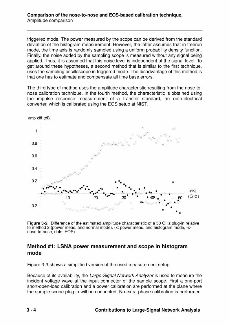
Comparison of the nose-to-nose and EOS-based calibration technique.Amplitude comparison
3 - 4 Contributions to Large-Signal Network Analysis
triggered mode. The power measured by the scope can be derived from the standarddeviation of the histogram measurement. However, the latter assumes that in freerunmode, the time axis is randomly sampled using a uniform probability density function.Finally, the noise added by the sampling scope is measured without any signal beingapplied. Thus, it is assumed that this noise level is independent of the signal level. Toget around these hypotheses, a second method that is similar to the first technique,uses the sampling oscilloscope in triggered mode. The disadvantage of this method isthat one has to estimate and compensate all time base errors.
The third type of method uses the amplitude characteristic resulting from the nose-to-nose calibration technique. In the fourth method, the characteristic is obtained usingthe impulse response measurement of a transfer standard, an opto-electricalconverter, which is calibrated using the EOS setup at NIST.
Method #1: LSNA power measurement and scope in histogram mode
Figure 3-3 shows a simplified version of the used measurement setup.
Because of its availability, the Large-Signal Network Analyzer is used to measure theincident voltage wave at the input connector of the sample scope. First a one-portshort-open-load calibration and a power calibration are performed at the plane wherethe sample scope plug-in will be connected. No extra phase calibration is performed.
Figure 3-2. Difference of the estimated amplitude characteristic of a 50 GHz plug-in relative to method 2 (power meas. and normal mode). (x: power meas. and histogram mode, -x-: nose-to-nose, dots: EOS).
10 20 30 40 50
freqGHz
0.2
0.2
0.4
0.6
0.8
1
amp diff dB
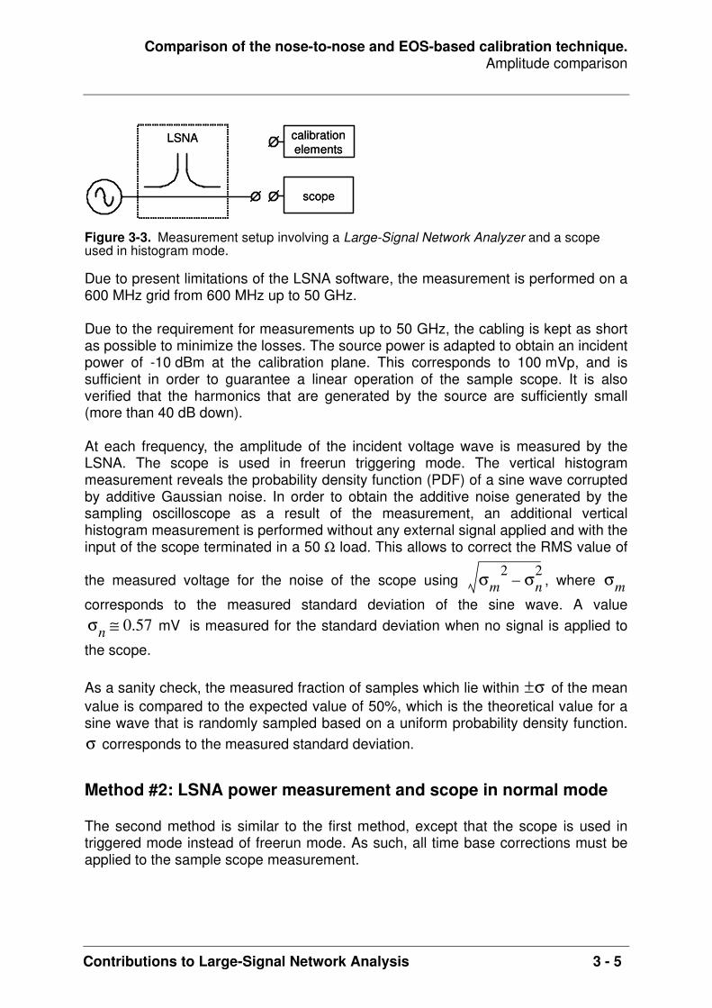
Comparison of the nose-to-nose and EOS-based calibration technique.Amplitude comparison
Contributions to Large-Signal Network Analysis 3 - 5
Due to present limitations of the LSNA software, the measurement is performed on a600 MHz grid from 600 MHz up to 50 GHz.
Due to the requirement for measurements up to 50 GHz, the cabling is kept as shortas possible to minimize the losses. The source power is adapted to obtain an incidentpower of -10 dBm at the calibration plane. This corresponds to 100 mVp, and issufficient in order to guarantee a linear operation of the sample scope. It is alsoverified that the harmonics that are generated by the source are sufficiently small(more than 40 dB down).
At each frequency, the amplitude of the incident voltage wave is measured by theLSNA. The scope is used in freerun triggering mode. The vertical histogrammeasurement reveals the probability density function (PDF) of a sine wave corruptedby additive Gaussian noise. In order to obtain the additive noise generated by thesampling oscilloscope as a result of the measurement, an additional verticalhistogram measurement is performed without any external signal applied and with theinput of the scope terminated in a 50 Ω load. This allows to correct the RMS value of
the measured voltage for the noise of the scope using , where
corresponds to the measured standard deviation of the sine wave. A value is measured for the standard deviation when no signal is applied to
the scope.
As a sanity check, the measured fraction of samples which lie within of the meanvalue is compared to the expected value of 50%, which is the theoretical value for asine wave that is randomly sampled based on a uniform probability density function.
corresponds to the measured standard deviation.
Method #2: LSNA power measurement and scope in normal mode
The second method is similar to the first method, except that the scope is used intriggered mode instead of freerun mode. As such, all time base corrections must beapplied to the sample scope measurement.
Figure 3-3. Measurement setup involving a Large-Signal Network Analyzer and a scope used in histogram mode.
calibrationelements
LSNA
scope
calibrationelements
LSNA
scope
σm2 σn
2– σm
σn 0.57 mV≅
σ±
σ

Comparison of the nose-to-nose and EOS-based calibration technique.Amplitude comparison
3 - 6 Contributions to Large-Signal Network Analysis
First, a time base distortion measurement is performed. Subtle effects like the thermaltail1 must be properly dealt with. Therefore, both the trigger rate and the time baseresolution are selected to be identical during the measurements that are used toestimate the time base distortion and during the actual measurements. In order toavoid leakage after time base distortion correction, the width of the selectedacquisition window must equal an integer number of periods. All applied frequenciesare an integer multiple of 600 MHz and therefore an acquisition window width of 5 nsis selected.
The time base drift estimation and the time base distortion correction are based on themethods described in the “Enhancements to the nose-to-nose calibration technique”chapter. Figure 3-4 shows the spectrum before time base distortion correction, basedon the sample mean of 500 measured records of 4000 points each. The mean iscalculated after time base drift estimation and compensation. The amplitude at48 GHz is found to be -14.57 dBm. Figure 3-5 shows the spectrum after time basedistortion correction. The amplitude at 48 GHz is now found to be -13.05 dBm. Thisdemonstrates that a bias of 1.5 dB is introduced when one neglects the time basedistortion. Figure 3-5 reveals a strange residual shaping of the spectrum around48 GHz. Comparing the time signal to the pure sine wave based on the amplitude andphase at 48 GHz (figure 3-6) clearly shows some small residual “thermal tail” effect,which is assumed to be caused by small temperature variations in between the timebase distortion measurements and the measurements at 48 GHz.
1. described in the “Enhancements to the nose-to-nose calibration technique” chapter.
Figure 3-4. Measured averaged spectrum before time base distortion correction (48 GHz).
20 40 60 80 100freq GHz
80
70
60
50
40
30
20
10ampl dBm
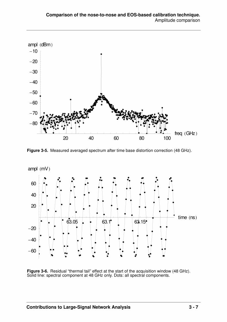
Comparison of the nose-to-nose and EOS-based calibration technique.Amplitude comparison
Contributions to Large-Signal Network Analysis 3 - 7
Figure 3-5. Measured averaged spectrum after time base distortion correction (48 GHz).
Figure 3-6. Residual “thermal tail” effect at the start of the acquisition window (48 GHz).Solid line: spectral component at 48 GHz only. Dots: all spectral components.
20 40 60 80 100freq GHz
80
70
60
50
40
30
20
10ampl dBm
63.05 63.1 63.15time ns
60
40
20
20
40
60
ampl mV
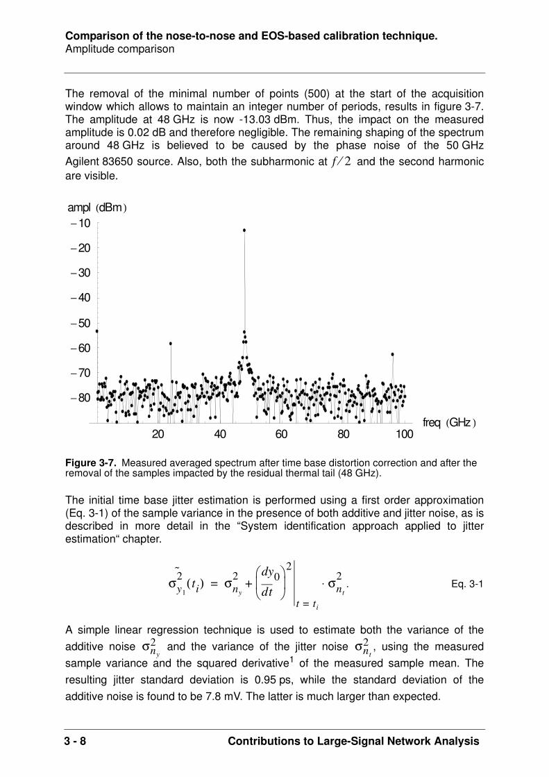
Comparison of the nose-to-nose and EOS-based calibration technique.Amplitude comparison
3 - 8 Contributions to Large-Signal Network Analysis
The removal of the minimal number of points (500) at the start of the acquisitionwindow which allows to maintain an integer number of periods, results in figure 3-7.The amplitude at 48 GHz is now -13.03 dBm. Thus, the impact on the measuredamplitude is 0.02 dB and therefore negligible. The remaining shaping of the spectrumaround 48 GHz is believed to be caused by the phase noise of the 50 GHzAgilent 83650 source. Also, both the subharmonic at and the second harmonicare visible.
The initial time base jitter estimation is performed using a first order approximation(Eq. 3-1) of the sample variance in the presence of both additive and jitter noise, as isdescribed in more detail in the “System identification approach applied to jitterestimation“ chapter.
. Eq. 3-1
A simple linear regression technique is used to estimate both the variance of theadditive noise and the variance of the jitter noise , using the measuredsample variance and the squared derivative1 of the measured sample mean. Theresulting jitter standard deviation is 0.95 ps, while the standard deviation of theadditive noise is found to be 7.8 mV. The latter is much larger than expected.
Figure 3-7. Measured averaged spectrum after time base distortion correction and after the removal of the samples impacted by the residual thermal tail (48 GHz).
f 2⁄
20 40 60 80 100freq GHz
80
70
60
50
40
30
20
10ampl dBm
σy1
2 ti( ) σny
2td
dy0
2
t ti=
σnt
2⋅+=
σny
2 σnt
2
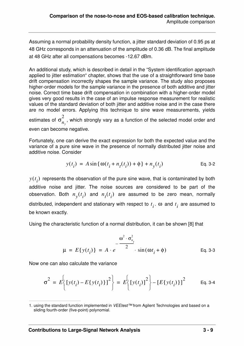
Comparison of the nose-to-nose and EOS-based calibration technique.Amplitude comparison
Contributions to Large-Signal Network Analysis 3 - 9
Assuming a normal probability density function, a jitter standard deviation of 0.95 ps at48 GHz corresponds in an attenuation of the amplitude of 0.36 dB. The final amplitudeat 48 GHz after all compensations becomes -12.67 dBm.
An additional study, which is described in detail in the “System identification approachapplied to jitter estimation“ chapter, shows that the use of a straightforward time basedrift compensation incorrectly shapes the sample variance. The study also proposeshigher-order models for the sample variance in the presence of both additive and jitternoise. Correct time base drift compensation in combination with a higher-order modelgives very good results in the case of an impulse response measurement for realisticvalues of the standard deviation of both jitter and additive noise and in the case thereare no model errors. Applying this technique to sine wave measurements, yields
estimates of , which strongly vary as a function of the selected model order and
even can become negative.
Fortunately, one can derive the exact expression for both the expected value and thevariance of a pure sine wave in the presence of normally distributed jitter noise andadditive noise. Consider
Eq. 3-2
represents the observation of the pure sine wave, that is contaminated by both
additive noise and jitter. The noise sources are considered to be part of theobservation. Both and are assumed to be zero mean, normally
distributed, independent and stationary with respect to . and are assumed to
be known exactly.
Using the characteristic function of a normal distribution, it can be shown [8] that
Eq. 3-3
Now one can also calculate the variance
Eq. 3-4
1. using the standard function implemented in VEEtest™ from Agilent Technologies and based on a sliding fourth-order (five-point) polynomial.
σny
2
y ti( ) A ω ti nt ti( )+( ) φ+ sin ny ti( )+=
y ti( )
ny ti( ) nt ti( )
ti ω ti
µ E y ti( ) A e
ω2 σnt
2⋅
2-----------------–
ωti φ+( )sin⋅ ⋅= =
σ2 E y ti( ) E y ti( ) –[ ]2
E y ti( )[ ]2
E y ti( ) [ ]2–= =

Comparison of the nose-to-nose and EOS-based calibration technique.Amplitude comparison
3 - 10 Contributions to Large-Signal Network Analysis
The first term in this expression is found to be:
Eq. 3-5
Combining equations Eq. 3-3 up to Eq. 3-5, one obtains the value of the variance:
Eq. 3-6
In the absence of time base distortion, one can easily retrieve the values of , ,
and using the Fourier transform of Eq. 3-3 and Eq. 3-6.
When time base distortion is present, as is the case during our measurements, one
can obtain an estimate for , , and by minimizing the following cost
function with respect to these unknowns:
Eq. 3-7
E A ω ti nt ti( )+( ) φ+ sin ny ti( )+[ ]2
A2
2------ A2
2------ E 2ω ti nt ti( )+( ) 2φ+[ ]cos ⋅ σny
2+–=
A2
2------ A
2
2------ e
2ω( )2 σnt
2⋅
2--------------------------–
2 ωti φ+( )[ ]cos⋅ ⋅ σny
2+–=
A2E ω ti nt ti( )+( ) φ+ sin[ ]2
σny
2+=
σ2 σny
2 A2
2------ 1 e
ω2 σnt
2⋅––
1 eω2 σnt
2⋅–2 ωti φ+( )[ ]cos⋅+
+=
A φ σny
2
σnt
2
A φ σny
2 σnt
2
V W( )LS1
Wi2
------- σi2 σny
2– A2
2------ 1 e
ω2 σnt
2⋅––
1 eω2 σnt
2⋅–2ωti( )cos⋅+
–
2
i 1=
N
=
1
Wi'2
---------- µi A e
ω2 σnt
2⋅
2-----------------–
ωti φ+( )sin⋅ ⋅–
2
i 1=
N
+
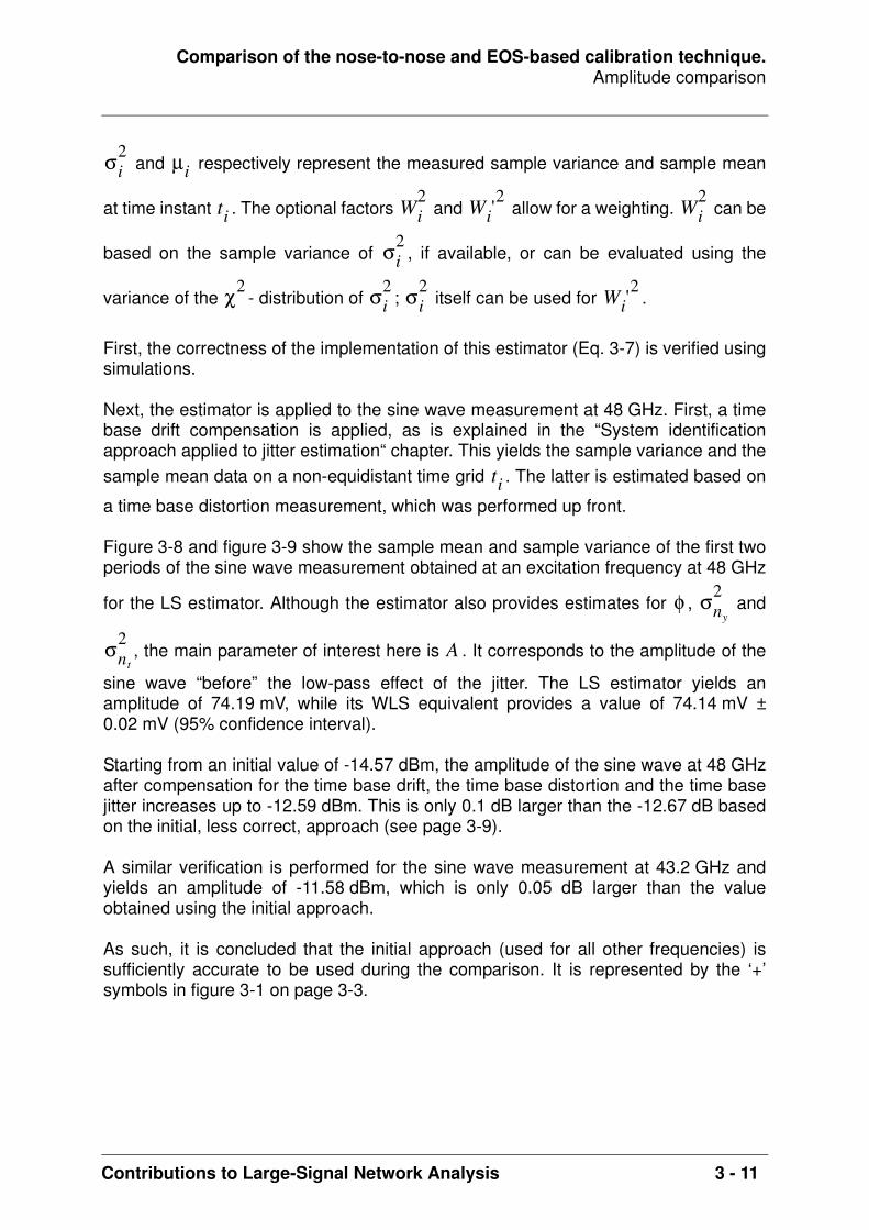
Comparison of the nose-to-nose and EOS-based calibration technique.Amplitude comparison
Contributions to Large-Signal Network Analysis 3 - 11
and respectively represent the measured sample variance and sample mean
at time instant . The optional factors and allow for a weighting. can be
based on the sample variance of , if available, or can be evaluated using the
variance of the - distribution of ; itself can be used for .
First, the correctness of the implementation of this estimator (Eq. 3-7) is verified usingsimulations.
Next, the estimator is applied to the sine wave measurement at 48 GHz. First, a timebase drift compensation is applied, as is explained in the “System identificationapproach applied to jitter estimation“ chapter. This yields the sample variance and thesample mean data on a non-equidistant time grid . The latter is estimated based on
a time base distortion measurement, which was performed up front.
Figure 3-8 and figure 3-9 show the sample mean and sample variance of the first twoperiods of the sine wave measurement obtained at an excitation frequency at 48 GHz
for the LS estimator. Although the estimator also provides estimates for , and
, the main parameter of interest here is . It corresponds to the amplitude of the
sine wave “before” the low-pass effect of the jitter. The LS estimator yields anamplitude of 74.19 mV, while its WLS equivalent provides a value of 74.14 mV ±0.02 mV (95% confidence interval).
Starting from an initial value of -14.57 dBm, the amplitude of the sine wave at 48 GHzafter compensation for the time base drift, the time base distortion and the time basejitter increases up to -12.59 dBm. This is only 0.1 dB larger than the -12.67 dB basedon the initial, less correct, approach (see page 3-9).
A similar verification is performed for the sine wave measurement at 43.2 GHz andyields an amplitude of -11.58 dBm, which is only 0.05 dB larger than the valueobtained using the initial approach.
As such, it is concluded that the initial approach (used for all other frequencies) issufficiently accurate to be used during the comparison. It is represented by the ‘+’symbols in figure 3-1 on page 3-3.
σi2 µi
ti Wi2
Wi'2
Wi2
σi2
χ2 σi2 σi
2 Wi'2
ti
φ σny
2
σnt
2A

Comparison of the nose-to-nose and EOS-based calibration technique.Amplitude comparison
3 - 12 Contributions to Large-Signal Network Analysis
Figure 3-8. First two periods of the measured sample mean at 48 GHz (black dots), its 95% confidence interval (vertical black lines) and the estimated mean (red solid line).
Figure 3-9. Corresponding measured sample variance at 48 GHz (black dots), its 95% confidence interval (vertical black lines) and the estimated variance (red solid line).
0.01 0.02 0.03 0.04time ns
60
40
20
20
40
60
mean mV
0.01 0.02 0.03 0.04time ns
0.2
0.4
0.6
0.8
var x103 V2
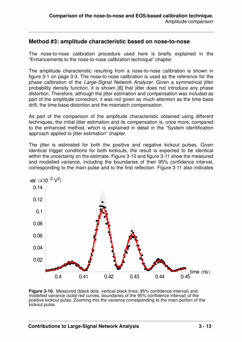
Comparison of the nose-to-nose and EOS-based calibration technique.Amplitude comparison
Contributions to Large-Signal Network Analysis 3 - 13
Method #3: amplitude characteristic based on nose-to-nose
The nose-to-nose calibration procedure used here is briefly explained in the“Enhancements to the nose-to-nose calibration technique” chapter.
The amplitude characteristic resulting from a nose-to-nose calibration is shown infigure 3-1 on page 3-3. The nose-to-nose calibration is used as the reference for thephase calibration of the Large-Signal Network Analyzer. Given a symmetrical jitterprobability density function, it is shown [8] that jitter does not introduce any phasedistortion. Therefore, although the jitter estimation and compensation was included aspart of the amplitude correction, it was not given as much attention as the time basedrift, the time base distortion and the mismatch compensation.
As part of the comparison of the amplitude characteristic obtained using differenttechniques, the initial jitter estimation and its compensation is, once more, comparedto the enhanced method, which is explained in detail in the “System identificationapproach applied to jitter estimation“ chapter.
The jitter is estimated for both the positive and negative kickout pulses. Givenidentical trigger conditions for both kickouts, the result is expected to be identicalwithin the uncertainty on the estimate. Figure 3-10 and figure 3-11 show the measuredand modelled variance, including the boundaries of their 95% confidence interval,corresponding to the main pulse and to the first reflection. Figure 3-11 also indicates
Figure 3-10. Measured (black dots, vertical black lines: 95% confidence interval) and modelled variance (solid red curves, boundaries of the 95% confidence interval) of the positive kickout pulse. Zooming into the variance corresponding to the main portion of the kickout pulse.
0.4 0.41 0.42 0.43 0.44 0.45time ns
0.02
0.04
0.06
0.08
0.1
0.12
0.14var x103 V2

Comparison of the nose-to-nose and EOS-based calibration technique.Amplitude comparison
3 - 14 Contributions to Large-Signal Network Analysis
that the model is also capable to model the variance of the additive noise. A leastsquare estimator is used in combination with a third order model because the jitterstandard deviation exceeds 1 ps. The rationale of this decision and the details of thejitter estimation are explained in the “System identification approach applied to jitterestimation“ chapter.
The estimate of the jitter standard deviation for the positive kickout pulse is found tobe 1.383 ps ± 21 fs (95% confidence interval). The estimate of the jitter standarddeviation for the negative kickout pulse is found to be 1.385 ps ± 19 fs and equals thatof the positive kickout within the 95% confidence interval.
Figure 3-12 shows the relative difference (in dB) of the amplitude characteristic of theM12 measurement1 after time base drift and time base jitter estimation and dittocompensation, based on the original and the new approach. The new approach givesa slightly larger amplitude at 50 GHz.
Given a difference of 80 mdB at 50 GHz, it can be concluded that the originalapproach is sufficiently accurate to be used during the actual comparison of theamplitude characteristic of the 50 GHz plug-in.
Figure 3-11. Measured (black dots, vertical black lines: 95% confidence interval) and modelled variance (solid red curves, boundaries of the 95% confidence interval) of the positive kickout pulse. Zooming into the variance corresponding to the first reflection of the kickout pulse.
1. the M12 measurement uses plug-in 2 as kickout generator and plug-in 1 as kickout receiver.
1.4 1.45 1.5 1.55 1.6 1.65time ns
0.2
0.4
0.6
0.8
1
var x106 V2

Comparison of the nose-to-nose and EOS-based calibration technique.Amplitude comparison
Contributions to Large-Signal Network Analysis 3 - 15
Method #4: amplitude characteristic based on EOS
The last method uses an opto-electrical (O/E) converter which is calibrated up to110 GHz using the electro-optical sampling system [1]-[4] at NIST as a referenceelement. This O/E converter is then used in the setup described in figure 3-13. Thecalibrated O/E converter is excited by an optical impulse. After compensating for alltime base effects and mismatch effects, the impulse response measured by thesampling scope equals the convolution of the (known) impulse response of the O/Eand the (unknown) impulse response of the sampling oscilloscope plug-in. As theimpulse response of the O/E is known, the latter can be obtained. The second O/E inthe trigger path is solely used to convert the optical pulse into an electrical pulse thatcan be used to trigger the sampling oscilloscope.
Figure 3-12. Relative difference between the estimated plug-in amplitude characteristic based on the new time base drift and jitter compensation and the original implementation.
Figure 3-13. Block diagram of the setup used during the sampling oscilloscope calibration using a EOS-calibrated O/E converter.
10 20 30 40 50freq GHz
0.02
0.04
0.06
0.08
difference dB
impulselaser
calibratedO/E
samplingoscilloscope
trigger2nd O/E
Ch1/3impulselaser
impulselaser
calibratedO/E
calibratedO/E
samplingoscilloscope
trigger2nd O/E
Ch1/3
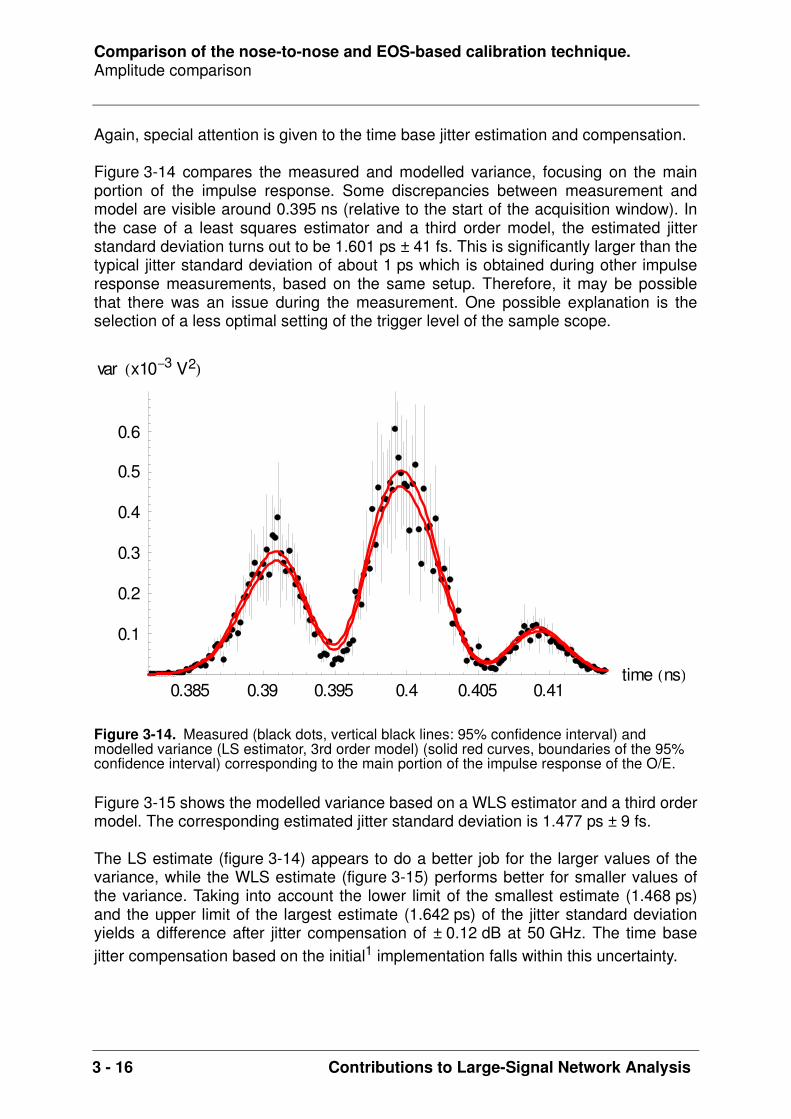
Comparison of the nose-to-nose and EOS-based calibration technique.Amplitude comparison
3 - 16 Contributions to Large-Signal Network Analysis
Again, special attention is given to the time base jitter estimation and compensation.
Figure 3-14 compares the measured and modelled variance, focusing on the mainportion of the impulse response. Some discrepancies between measurement andmodel are visible around 0.395 ns (relative to the start of the acquisition window). Inthe case of a least squares estimator and a third order model, the estimated jitterstandard deviation turns out to be 1.601 ps ± 41 fs. This is significantly larger than thetypical jitter standard deviation of about 1 ps which is obtained during other impulseresponse measurements, based on the same setup. Therefore, it may be possiblethat there was an issue during the measurement. One possible explanation is theselection of a less optimal setting of the trigger level of the sample scope.
Figure 3-15 shows the modelled variance based on a WLS estimator and a third ordermodel. The corresponding estimated jitter standard deviation is 1.477 ps ± 9 fs.
The LS estimate (figure 3-14) appears to do a better job for the larger values of thevariance, while the WLS estimate (figure 3-15) performs better for smaller values ofthe variance. Taking into account the lower limit of the smallest estimate (1.468 ps)and the upper limit of the largest estimate (1.642 ps) of the jitter standard deviationyields a difference after jitter compensation of ± 0.12 dB at 50 GHz. The time basejitter compensation based on the initial1 implementation falls within this uncertainty.
Figure 3-14. Measured (black dots, vertical black lines: 95% confidence interval) and modelled variance (LS estimator, 3rd order model) (solid red curves, boundaries of the 95% confidence interval) corresponding to the main portion of the impulse response of the O/E.
0.385 0.39 0.395 0.4 0.405 0.41time ns
0.1
0.2
0.3
0.4
0.5
0.6
var x103 V2

Comparison of the nose-to-nose and EOS-based calibration technique.Amplitude comparison
Contributions to Large-Signal Network Analysis 3 - 17
Summary
Although the comparison does not include any confidence intervals, figure 3-1 onpage 3-3 shows good correspondence between all methods, except for the nose-to-nose which seems too yield an amplitude characteristic which is consistently toolarge. A possible explanation can be found in [9]. The difference between the nose-to-nose and the other methods (see figure 3-2 on page 3-4) is very similar to thediscrepancy reported by NIST [6], both in shape and in order of magnitude. Thedifference is larger than can be contributed to differences in time base drift and timebase jitter correction.
1. less correct with respect to time base jitter estimation as explained in the “System identification approach applied to jitter estimation“ chapter.
Figure 3-15. Measured (black dots, vertical black lines: 95% confidence interval) and modelled variance (WLS estimator, 3rd order model) (solid red curves, boundaries of the 95% confidence interval) corresponding to the main portion of the impulse response of the O/E.
0.385 0.39 0.395 0.4 0.405 0.41time ns
0.1
0.2
0.3
0.4
0.5
0.6
var x103 V2
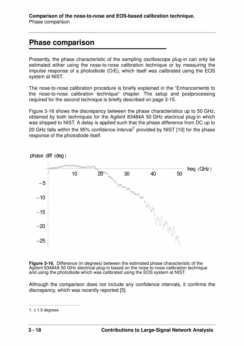
Comparison of the nose-to-nose and EOS-based calibration technique.Phase comparison
3 - 18 Contributions to Large-Signal Network Analysis
Phase comparison
Presently, the phase characteristic of the sampling oscilloscope plug-in can only beestimated either using the nose-to-nose calibration technique or by measuring theimpulse response of a photodiode (O/E), which itself was calibrated using the EOSsystem at NIST.
The nose-to-nose calibration procedure is briefly explained in the “Enhancements tothe nose-to-nose calibration technique” chapter. The setup and postprocessingrequired for the second technique is briefly described on page 3-15.
Figure 3-16 shows the discrepancy between the phase characteristics up to 50 GHz,obtained by both techniques for the Agilent 83484A 50 GHz electrical plug-in whichwas shipped to NIST. A delay is applied such that the phase difference from DC up to20 GHz falls within the 95% confidence interval1 provided by NIST [10] for the phaseresponse of the photodiode itself.
Although the comparison does not include any confidence intervals, it confirms thediscrepancy, which was recently reported [5].
1. ± 1.5 degrees
Figure 3-16. Difference (in degrees) between the estimated phase characteristic of the Agilent 83484A 50 GHz electrical plug-in based on the nose-to-nose calibration technique and using the photodiode which was calibrated using the EOS system at NIST.
10 20 30 40 50freq GHz
25
20
15
10
5
phase diff deg
Comparison of the nose-to-nose and EOS-based calibration technique.Conclusions
Contributions to Large-Signal Network Analysis 3 - 19
Conclusions
The performed comparisons confirm the discrepancies which were reported, both withrespect to the amplitude characteristic and the phase characteristic of a 50 GHzelectrical plug-in, obtained after a nose-to-nose calibration.
Finding an explanation for this discrepancy is left as topic for future research. Fitting aparametric model on the amplitude and phase discrepancy may provide some insight.Also, it makes sense to mention that [11] reports a much better correspondence forthe amplitude characteristic of a sampler up to 120 GHz, based on a nose-to-nosecalibration and a power measurement.
Eq. 3-6 gives the exact expression of the variance for a sine wave which is disturbedby both additive and jitter noise, in the case the latter has a normal probability densityfunction. It is a rather small effort to provide the exact expression for otherdistributions, based on [8].
Comparison of the nose-to-nose and EOS-based calibration technique.References
3 - 20 Contributions to Large-Signal Network Analysis
References
[1] D. Williams, P. Hale, T. Clement, and J. Morgan, "Mismatch corrections for electro-optic sampling systems," 56th ARFTG Conference Digest, pp. 141-145, Nov. 30-Dec.1, 2000[2] D. Williams, P. Hale, T. Clement, and J. Morgan, "Calibrating electro-optic sam-pling systems," Int. Microwave Symposium Digest, Phoenix, AZ, pp. 1527-1530, May20-25, 2001[3] T. Clement, D. Williams, P. Hale, and J. Morgan, "Calibrating photoreceiverresponse to 110 GHz," Proc. 15th Annual Meeting, IEEE Lasers and Electro-opticsSoc., Glasgow, Scotland, 2002[4] D. Williams, P. Hale, T. Clement, C-M. Wang, "Uncertainty of the NIST Electro-optic Sampling System," NIST Technical Note 1535, 2004[5] D. Williams, P. Hale, T. Clement, “Electrical-phase Traceability to NIST’s EOS Sys-tem,” research update presented at the 4th ARFTG NVNA User’s Forum, June 2004(http://www.arftg.org/LSNA/4th/UsersForum_June2004_Minutes2.pdf)[6] P. Hale, T. Clement, K. Coakley, C. Wand, D. DeGroot and A. Verdoni, “Estimatingthe Magnitude and Phase Response of a 50 GHz Sampling Oscilloscope Using the“Nose-To-Nose” Method”, 55th ARFTG Conf. Digest, June 2000.[7] Marc Vanden Bossche, private communication 2005.[8] T. Souders, D. Flach, C. Hagwood and G. Yang, “The Effects of Timing Jitter inSampling Systems,” IEEE Transactions on Instrumentation and Measurement, Vol.39, No. 1, February 1990[9] K. Remley, “The Impact of Internal Sampling Circuitry on the Phase Error of theNose-to-Nose Oscilloscope Calibration”, NIST Technical Note 1528.[10] T. Clement, P. Hale and D. Williams, “Report of special test (42161S)”, NIST IDnumber 814627.[11] J. Scott, "Rapid Millimetre-wave Sampler Response Characterization to WellBeyond 120 GHz Using an Improved Nose-to-nose Method," Int. Microwave Sympo-sium Digest, Philadelphia, pp. 1511-1514, June 2003

Contributions to Large-Signal Network Analysis 4 - 1
• “Abstract” on page 4-2
• “Modeling variance in the presence of additive and jitter noise” on page 4-3
• “Estimators” on page 4-6
• “Generation of simulation data” on page 4-12
• “Step 1: third order approximation of variance, known derivatives” on page 4-17
• “Step 2: realistic variance, known derivatives” on page 4-27
• “Step 3: realistic variance, derivatives based on sample mean” on page 4-36
• “Step 4: influence of time base drift” on page 4-44
• “Step 5: measurements” on page 4-50
• “Conclusions” on page 4-66
• “References” on page 4-67
CHAPTER 4 System identification approach applied to jitter estimation.

System identification approach applied to jitter estimation.Abstract
4 - 2 Contributions to Large-Signal Network Analysis
Abstract
Given a symmetrical probability density function, jitter does not introduce phasedistortion [1]. However, it has a low-pass effect on the amplitude characteristic.Because the nose-to-nose calibration procedure was mainly used to provide phaseinformation, initially jitter estimation was of less importance.
However, the crossverification of the amplitude distortion of a 50 GHz samplingoscilloscope based on the nose-to-nose calibration technique and the electro-opticsampling system of NIST, justifies additional research with respect to jitter estimation.
A system identification1 approach is applied to estimate the jitter introduced by a high-frequency sampling oscilloscope.
First, an extended model is proposed to describe the sample variance of a set ofrepeated (impulse response) measurements in the presence of additive and jitternoise. It is important to remember that the primary goal in this work is to estimate thejitter and as such not the deterministic part of the system, i.e. the impulse response.
Next, the (weighted) least-squares and maximum likelihood estimator are introduced.
Results are shown based on simulations. First, the simulated variance is based on aknown model, involving both jitter and additive noise. This allows to test both thecorrectness of the implementations and to verify the ability to detect model errors.Next, more realistic simulations are performed using “real” jitter. The simulations alsoallow to study the effect of uncertainties on the input signal. More specifically, first theexact derivatives of the exact signal are used, while in a next step, these derivativesare calculated from the sample mean of the signal.
Finally, the jitter and additive noise standard deviation are estimated on realmeasurements by performing impulse response measurements using an Agilent83480A sampling oscilloscope in combination with 83484A 50 GHz electrical plug-ins.Additional challenges, such as the conjugated effect of time base drift and time basedistortion, are described and correctly taken care of, demonstrating the real power of asolid stochastical framework.
1. “The aim of identification theory is to provide a systematic approach to fit a mathematical model, as well as possible, to the deterministic part of the system, eliminating the noise distortions as much as possible.” (extracted from “An Introduction to System Identification”, Prof. J. Schoukens, published by the Vrije Universiteit Brussel)

System identification approach applied to jitter estimation.Modeling variance in the presence of additive and jitter noise
Contributions to Large-Signal Network Analysis 4 - 3
Modeling variance in the presence of additive and jitter noise
High-frequency sampling oscilloscopes often use an equivalent-time samplingprinciple and suffer from both additive measurement noise and timing jitter
noise at the sampling time instance .
Eq. 4-1
represents the measurement of the exact signal when both additive
noise and jitter are added as part of the measurement. Both and are
assumed to be zero mean, normally distributed1, independent and stationary withrespect to .
In general it is assumed that the time jitter is small compared to the characteristic timeconstant2 of the exact signal . In that case is approximated by
its first order Taylor series approximation:
Eq. 4-2
Given zero mean additive and jitter noise, the expected value of equals
and it makes sense to note that this first order approximation cannot explain the low-pass effect introduced by jitter.
Furthermore, the variance of equals
1. Extract of a private communication with Bernie Hovden, Technical Support Engineer Digital Signal Analysis of Agilent Technologies in Santa Rosa to support the assumption of a normal distribution of the jitter in the case of the Agilent 83480A sampling oscilloscope from a hardware point of view:“The inherent trigger jitter in the 83480A basically comes from the translation of amplitude noise (which is typically Gaussian) on the finite rise time trigger source to time in the trigger and time base circuits from the recognition of a trigger event to the firing of the sampler. The decision circuit typically operates over a linear part of the transition so the converted noise should remain Gaussian. Both the trigger and time base circuits have multiple independent stages where the threshold detection takes place sequentially, with no synchronization between the stages. An educated guess is that there are at least 14 separate translations of amplitude to time. The central limit theorem says that a large number of independent events with uncertainties will tend to a Gaussian PDF.”
2. defined as in case of an impulse response or in case of a multi-tone
ny ti( )
nt ti( ) ti
y ti( ) y0 ti nt ti( )+( ) ny ti( )+=
y ti( ) y0 ti( )
ny ti( ) nt ti( )
t
y0 ti( ) y0 ti nt ti( )+( )
1 ω 3dB–⁄ 1 ωmax⁄
y1˜ ti( ) y0 ti( )
td
dy0
t ti=nt ti( )⋅ ny ti( )+ +=
y1˜ ti( ) y0 ti( )
y1˜ ti( )
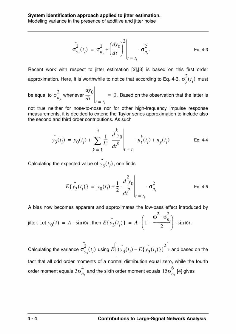
System identification approach applied to jitter estimation.Modeling variance in the presence of additive and jitter noise
4 - 4 Contributions to Large-Signal Network Analysis
. Eq. 4-3
Recent work with respect to jitter estimation [2],[3] is based on this first order
approximation. Here, it is worthwhile to notice that according to Eq. 4-3, must
be equal to whenever . Based on the observation that the latter is
not true neither for nose-to-nose nor for other high-frequency impulse responsemeasurements, it is decided to extend the Taylor series approximation to include alsothe second and third order contributions. As such
Eq. 4-4
Calculating the expected value of , one finds
Eq. 4-5
A bias now becomes apparent and approximates the low-pass effect introduced by
jitter. Let , then .
Calculating the variance using and based on the
fact that all odd order moments of a normal distribution equal zero, while the fourth
order moment equals and the sixth order moment equals [4] gives
σy1
2ti( ) σny
2td
dy0
2
t ti=
σnt
2⋅+=
σy2 ti( )
σny
2td
dy0
t ti=0=
y3˜ ti( ) y0 ti( ) 1
k!----
tk
k
d
d y0
t ti=
ntk
ti( )⋅ ⋅
k 1=
3
ny ti( )+ +=
y3˜ ti( )
E y3˜ ti( ) y0 ti( ) 1
2---
t2
2
d
d y0
t ti=
σnt
2⋅ ⋅+=
y0 t( ) A ωtsin⋅= E y3˜ ti( ) A 1
ω2 σnt
2⋅
2-------------------–
ωtsin⋅ ⋅=
σy3
2 ti( ) E y3˜ ti( ) E y3
˜ ti( ) –( )2
3σnt
415σnt
6
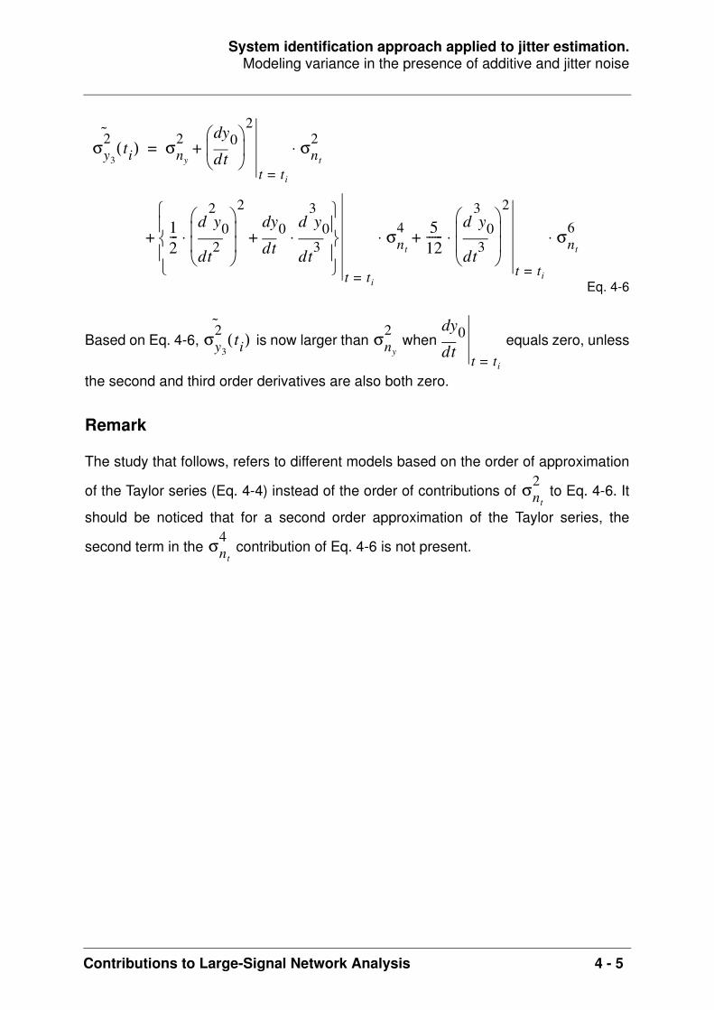
System identification approach applied to jitter estimation.Modeling variance in the presence of additive and jitter noise
Contributions to Large-Signal Network Analysis 4 - 5
Eq. 4-6
Based on Eq. 4-6, is now larger than when equals zero, unless
the second and third order derivatives are also both zero.
Remark
The study that follows, refers to different models based on the order of approximation
of the Taylor series (Eq. 4-4) instead of the order of contributions of to Eq. 4-6. It
should be noticed that for a second order approximation of the Taylor series, the
second term in the contribution of Eq. 4-6 is not present.
σy3
2 ti( ) σny
2td
dy0
2
t ti=
σnt
2⋅+=
12---
t2
2
d
d y0
2
⋅td
dy0
t3
3
d
d y0⋅+
t ti=
σnt
4⋅ 512------
t3
3
d
d y0
2
t ti=
σnt
6⋅ ⋅+ +
σy3
2ti( ) σny
2
td
dy0
t ti=
σnt
2
σnt
4
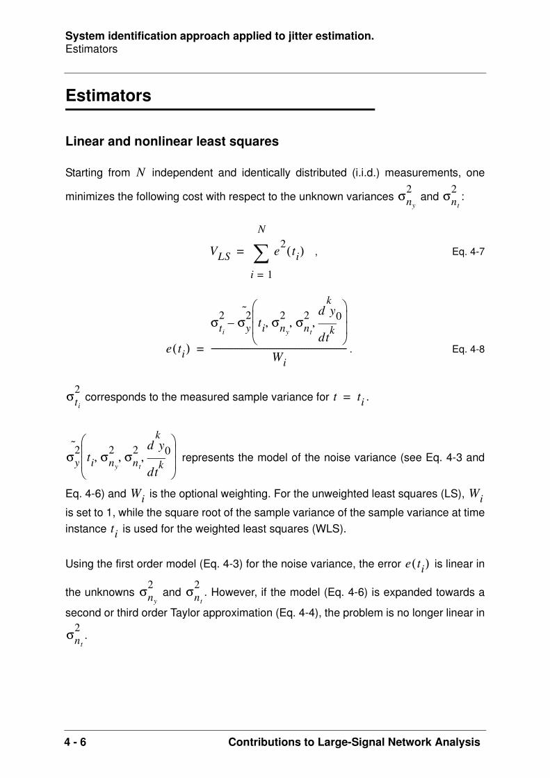
System identification approach applied to jitter estimation.Estimators
4 - 6 Contributions to Large-Signal Network Analysis
Estimators
Linear and nonlinear least squares
Starting from independent and identically distributed (i.i.d.) measurements, one
minimizes the following cost with respect to the unknown variances and :
, Eq. 4-7
. Eq. 4-8
corresponds to the measured sample variance for .
represents the model of the noise variance (see Eq. 4-3 and
Eq. 4-6) and is the optional weighting. For the unweighted least squares (LS),
is set to 1, while the square root of the sample variance of the sample variance at timeinstance is used for the weighted least squares (WLS).
Using the first order model (Eq. 4-3) for the noise variance, the error is linear in
the unknowns and . However, if the model (Eq. 4-6) is expanded towards a
second or third order Taylor approximation (Eq. 4-4), the problem is no longer linear in
.
N
σny
2 σnt
2
VLS e2 ti( )
i 1=
N
=
e ti( )
σti
2 σy2˜ ti σny
2 σnt
2
tk
k
d
d y0, , ,
–
Wi---------------------------------------------------------------=
σti
2t ti=
σy2˜ ti σny
2 σnt
2
tk
k
d
d y0, , ,
Wi Wi
ti
e ti( )
σny
2 σnt
2
σnt
2

System identification approach applied to jitter estimation.Estimators
Contributions to Large-Signal Network Analysis 4 - 7
Maximum Likelihood (ML) estimator
In [2] it is shown that the ML estimator produces statistically more efficient estimates
for and than a linear least squares estimator, assuming that the
model equals
Eq. 4-9
and corresponds to the exact model.
This estimator uses the knowledge that if each stochastical variable has a
normal distribution with unity variance and zero mean, then has a
chi-squared distribution with degrees of freedom. If the mean value of is
unknown, the (sample) mean has to be calculated and the number of degrees offreedom has to be decreased by 1.
The model described by Eq. 4-6 is now used to extend the ML estimator described in[2].
First, we derive the ML estimator in more detail based on a first order model,
Eq. 4-10
Then the distribution of the modelled output is derived, based on the
observation that for and ,
. Eq. 4-11
The distribution can then be normalized as follows:
σny
2ti( ) σnt
2ti( )
σy1
2 ti( ) σny
2td
dy0
2
t ti=
σnt
2⋅+=
Xi
N 0 1,( ) Xi2
i 1=
r
χr2 r Xi
y1˜ ti( ) y0 ti( )
td
dy0
t ti=nt ti( )⋅ ny ti( )+ +=
y1˜ ti( )
nt ti( ) N 0 σnt,( )∼ ny ti( ) N 0 σny
,( )∼
y1˜ ti( ) N y0 ti( ) σny
2td
dy0
2
t ti=
σnt
2⋅+,
∼

System identification approach applied to jitter estimation.Estimators
4 - 8 Contributions to Large-Signal Network Analysis
Eq. 4-12
Acquiring realizations of at , representing the realization index, it follows
that
. Eq. 4-13
Eq. 4-13 assumes that is known.
Using the sample mean and sample variance of
, Eq. 4-14
Eq. 4-13 becomes
. Eq. 4-15
Let to simplify the notation.
In order to derive the log likelihood function, one starts from the chi-squaredprobability distribution function with degrees of freedom
yN ti( )y1˜ ti( ) y0 ti( )–
σny
2td
dy0
2
t ti=
σnt
2⋅+
----------------------------------------------------------- N 0 1,( )∼=
K y t ti= k
yN2 ti k,( )
k 1=
K
y ti k,( ) y0 ti( )– 2
σny
2td
dy0
2
t ti=
σnt
2⋅+
-------------------------------------------------------
k 1=
K
χK2∼=
y0 ti( )
σti
2y ti( )
σti
2 1K 1–------------- y ti k,( ) 1
K---- y ti l,( )
l 1=
K
⋅–
2
k 1=
K
⋅=
yN2 ti k,( )
k 1=
K
K 1–( ) σti
2⋅
σny
2td
dy0
2
t ti=
σnt
2⋅+
------------------------------------------------------- χ K 1–( )2∼=
n K 1–=
n

System identification approach applied to jitter estimation.Estimators
Contributions to Large-Signal Network Analysis 4 - 9
. Eq. 4-16
Here .
First the integrand of Eq. 4-16 is evaluated.
Substitution of and , representing the
model, leads to
.
When maximizing the log likelihood function with respect to the model parameters, theconstant terms can be omitted. As such, the log likelihood function to be maximizedequals
. Eq. 4-17
Based on i.i.d. measurements, the following cost needs to be minimized with
respect to and :
F χ2( ) 1
2n 2⁄ Γ n2--- ⋅
----------------------------- x
n2--- 1–
e
x–2-----
⋅ ⋅ xd0
χ2
=
xn σti
2⋅
σny
2td
dy0
2
t ti=
σnt
2⋅+
-------------------------------------------------------=
x' σti
2= α σny
2td
dy0
2
t ti=
σnt
2⋅+= α
1
2n 2⁄ Γ n
2--- ⋅
----------------------------- x
n2--- 1–
e
x–2-----
⋅ ⋅ xd 1
2n 2⁄ Γ n
2--- ⋅
----------------------------- n x'⋅α
-----------
n2--- 1–
e
n x'⋅–2α
--------------nα--- dx'⋅⋅ ⋅ ⋅=
fln n2--- 1– αln⋅– n x'⋅
2α----------- αln–– n
2---– αln x'
α---+
⋅= =
N
σny
2 σnt
2

System identification approach applied to jitter estimation.Estimators
4 - 10 Contributions to Large-Signal Network Analysis
. Eq. 4-18
As such, the MLE cost in case of a third order model becomes
where must be substituted using Eq. 4-6.
Also, it is straightforward to extend Eq. 4-18 to deal with situations where the numberof degrees of freedom varies with . The relevance of this extension will become clearin “Step 4: influence of time base drift” on page 4-44. Eq. 4-18 becomes
, Eq. 4-19
where corresponds to the number of degrees of freedom for .
Curiosity
During simulations it was found that the second term contributing to the MLE cost incase of a first order model (Eq. 4-18) always equals . At first, this was believed to bea programming error. However, it is proven here that in the solution, this contributionalways equals .
VML =
n2--- σny
2td
dy0
2
t ti=
σnt
2⋅+
lnσti
2
σny
2td
dy0
2
t ti=
σnt
2⋅+
-------------------------------------------------------+
i 1=
N
⋅
n2--- βln
σti
2
β------+
i 1=
N
⋅
β
i
VML =
ni2---- σny
2td
dy0
2
t ti=
σnt
2⋅+
lnσti
2
σny
2td
dy0
2
t ti=
σnt
2⋅+
-------------------------------------------------------+⋅
i 1=
N
ni t ti=
N
N

System identification approach applied to jitter estimation.Estimators
Contributions to Large-Signal Network Analysis 4 - 11
Let , while and are estimates of and by minimizing
the cost (Eq. 4-18).
Then Eq. 4-18 becomes to be minimized with
respect to and .
Eq. 4-20
Eq. 4-21
Multiplying Eq. 4-20 by and Eq. 4-21 by and adding both equations, the sum iszero in the solution.
, which proves that .
This is exactly the second term in the cost function (Eq. 4-18).
xi td
dy0
2
t ti=
= a b σny
2 σnt
2
a b xi⋅+( )lnσti
2
a b xi⋅+---------------------+
i 1=
N
a b
a∂∂ 0= 1
a b xi⋅+---------------------
σti
2
a b xi⋅+( )2----------------------------–
i 1=
N
⇔ 0=
b∂∂ 0=
xia b xi⋅+---------------------
σti
2xi⋅
a b xi⋅+( )2----------------------------–
i 1=
N
⇔ 0=
a b
1σti
2
a b xi⋅+---------------------–
i 1=
N
0=σti
2
σny
2td
dy0
2
t ti=
σnt
2⋅+
-------------------------------------------------------
i 1=
N
N=

System identification approach applied to jitter estimation.Generation of simulation data
4 - 12 Contributions to Large-Signal Network Analysis
Generation of simulation data
First the different models and estimators are tested using simulation data.
This data should be kept as realistic as possible. Therefore, the combined impulseresponse of a real-world opto-electrical converter (O/E) and a 50 GHz samplingoscilloscope is used as a starting point. Figure 4-1 shows the block diagram of therequired setup. The second O/E in the trigger path is solely used to convert the opticalpulse into an electrical pulse that can be used to trigger the sampling oscilloscope.
For the measurement of the impulse response, a time record of 5 ns is used starting at143 ns and 500 records of 4096 points are acquired. The data are corrected for timebase drift and time base distortion. The resulting averaged impulse response is shownin figure 4-2. Figure 4-3 shows the same information on a logarithmic scale.
Figure 4-4 zooms in to the main portion of the averaged pulse and its correspondingsample variance. It is clearly shown that at the time instants where the averaged pulse
Figure 4-1. Block diagram of the setup used during the impulse measurement.
Figure 4-2. Averaged impulse response.
impulselaser
calibratedO/E
samplingoscilloscope
trigger2nd O/E
Ch1/3impulselaser
impulselaser
calibratedO/E
calibratedO/E
samplingoscilloscope
trigger2nd O/E
Ch1/3
1 2 3 4 5time ns
0.02
0.02
0.04
0.06
0.08
meanV

System identification approach applied to jitter estimation.Generation of simulation data
Contributions to Large-Signal Network Analysis 4 - 13
has a zero slope, the variance is larger than the constant level at both sides of thepulse, which corresponds to the variance of the additive noise. This means that Eq. 4-9 does not correspond to the exact model for the measured jittered signal.
To further increase the S/N ratio of the test signal, a rectangular window is first appliedin the frequency domain. All frequency components up to the first transmission zero(located at about 70 GHz) are kept. The other lines are set to zero. In order to removethe small ringing at the edges in the time domain, an ad hoc window is applied theretoo.
The corresponding analytical expression for the time signal is then given by its Fourierseries
Eq. 4-22
and allows to calculate the exact derivatives. represents the real part of the
complex value . If the number of relevant spectral lines becomes too large, the
calculation of using Eq. 4-22 becomes very time consuming and a fastimplementation of the inverse Fourier transform is used instead. However, whensimulating jitter noise, the time samples are no longer on an equidistant grid. In orderto avoid the calculation using Eq. 4-22, a two step approach is used. First, theequidistant is evaluated on a sufficiently oversampled time grid and then cubic
Figure 4-3. Averaged impulse response (logarithmic scale).
1 2 3 4 5time ns
120
80
60
40
20mean dBV
x t( ) re X m( ) e j2πm ∆f t⋅ ⋅⋅
m 0=
M
=
re x( )x Mx t( )
x t( )

System identification approach applied to jitter estimation.Generation of simulation data
4 - 14 Contributions to Large-Signal Network Analysis
interpolation is used to obtain the value at . Given the above impulse
response, it was found that oversampling by a factor of 128 in combination with cubicinterpolation leads to an RMS value for the difference between the exact andinterpolated signal that is about 200 dB down with respect to the RMS value of thesignal.
Figure 4-4. Zooming into the main portion of the averaged impulse response and its variance.
0.44 0.46 0.48 0.5 0.52 0.54 0.56time ns
0.02
0.02
0.04
0.06
0.08
meanV
0.44 0.46 0.48 0.5 0.52 0.54 0.56time ns
0.1
0.2
0.3
0.4
var x103 V2
x t nt t( )+( )

System identification approach applied to jitter estimation.Generation of simulation data
Contributions to Large-Signal Network Analysis 4 - 15
Random number generator
Another critical element during simulation is the random number generator that isused to generate the noisy simulations. It was found that it makes sense to verify thefitness of the generator before questioning the correctness of the implementation ofthe model extraction. The latter is implemented in C in order to keep the simulationtime reasonable. For performance reasons, the Vector Statistical Library [5] includedin the Intel® Math Kernel Library is used.
Initially, the sample variance of the variance of the additive noise, estimated usingboth the MLE and WLS for different values of the variance of the jitter noise,consistently turned out to be approximately 50% smaller than the variance predictedby the corresponding element of the parameter covariance matrix.
It was found that this artifact was caused by a poor selection of the underlying basicrandom number generator. Replacing the 31-bit multiplicative congruential generator1
(MCG31m1) by a combined multiple recursive generator with two components oforder 3 (MRG32k3a) [5], this problem was solved. The main problem with the originalbasic random number generator is its relatively small period length with respect to therelatively large sampling.
The fitness of the random number generator is tested by calculating the sample meanand sample variance of realizations of the following cost
Eq. 4-23
where and respectively represent the sample mean and sample
variance of realizations of with , and
. As such and its expected value .
1. According to Intel MKL support, “MCG31 has a rather short period (~232) and is not recommended for applications demanding a large volume of random numbers.” The number of samples used during step 1 of the simulations (see page 4-21) is100 x 4096 x 200 x 250 ~= 2x 10¹⁰ while 232 ~= 4x 10⁹.The MRG32k3a pseudo-random generator has a period of ~2191 (~3x 1057).
Ne
VzNw j, Ns–( )
2
SNw j,2
--------------------------------
j 1=
Nt
=
zNw j, SNw j,2
Nw zj xij2
i 1=
Ns
= xij N 0 1,( )∼ i 1 .. Ns=
j 1 .. Nt= zj χNs
2∼ E zj Ns=

System identification approach applied to jitter estimation.Generation of simulation data
4 - 16 Contributions to Large-Signal Network Analysis
If is chosen large enough, then , its sample mean and sample
variance are known to be independent and [6] can be used to verify the properties ofthe sample mean and sample variance based on Eq. 4-23.
Eq. 4-24
Eq. 4-25
Eq. 4-24 and Eq. 4-25 represent the increase of the expected value and variance ofthe cost when replacing the exact variance of by its sample variance based on
real (non-complex) data sets.
If is chosen sufficiently large, then
Eq. 4-26
and one can calculate the 95% confidence intervals of its sample mean and sample
variance using the Student-t and distribution for realizations [7].
It was found that using the Box-Müller transformation [5] in combination with the 31-bitmultiplicative congruential generator (MCG31m1) of the Intel® Math Kernel Library didnot pass the 95% confidence interval test for , ,
and , while the combined multiple recursive generator with two
components of order 3 (MRG32k3a) did. As such the latter is used during simulation.
Ns zj N Ns 2Ns,( )∼
µV E V Nw 1–
Nw 3–---------------- Nt⋅= =
σV2
E V E V –( )2 Nw 1–( )3
Nw 3–( )2 Nw 5–( )⋅-------------------------------------------------- 2Nt⋅= =
zj Nw
Nt
V NNw 1–
Nw 3–---------------- Nt⋅
Nw 1–( )3
Nw 3–( )2Nw 5–( )⋅
-------------------------------------------------- 2Nt⋅,
∼
χ Ne 1–( )2
Ne
Ns 100= Nw 200= Nt 400=
Ne 500=
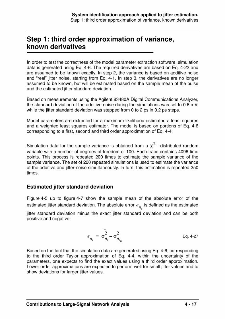
System identification approach applied to jitter estimation.Step 1: third order approximation of variance, known derivatives
Contributions to Large-Signal Network Analysis 4 - 17
Step 1: third order approximation of variance,known derivatives
In order to test the correctness of the model parameter extraction software, simulationdata is generated using Eq. 4-6. The required derivatives are based on Eq. 4-22 andare assumed to be known exactly. In step 2, the variance is based on additive noiseand “real” jitter noise, starting from Eq. 4-1. In step 3, the derivatives are no longerassumed to be known, but will be estimated based on the sample mean of the pulseand the estimated jitter standard deviation.
Based on measurements using the Agilent 83480A Digital Communications Analyzer,the standard deviation of the additive noise during the simulations was set to 0.6 mV,while the jitter standard deviation was stepped from 0 to 2 ps in 0.2 ps steps.
Model parameters are extracted for a maximum likelihood estimator, a least squaresand a weighted least squares estimator. The model is based on portions of Eq. 4-6corresponding to a first, second and third order approximation of Eq. 4-4.
Simulation data for the sample variance is obtained from a - distributed randomvariable with a number of degrees of freedom of 100. Each trace contains 4096 timepoints. This process is repeated 200 times to estimate the sample variance of thesample variance. The set of 200 repeated simulations is used to estimate the varianceof the additive and jitter noise simultaneously. In turn, this estimation is repeated 250times.
Estimated jitter standard deviation
Figure 4-5 up to figure 4-7 show the sample mean of the absolute error of theestimated jitter standard deviation. The absolute error is defined as the estimated
jitter standard deviation minus the exact jitter standard deviation and can be bothpositive and negative.
Eq. 4-27
Based on the fact that the simulation data are generated using Eq. 4-6, correspondingto the third order Taylor approximation of Eq. 4-4, within the uncertainty of theparameters, one expects to find the exact values using a third order approximation.Lower order approximations are expected to perform well for small jitter values and toshow deviations for larger jitter values.
χ2
ent
entσnt
2 σnt0
2–=
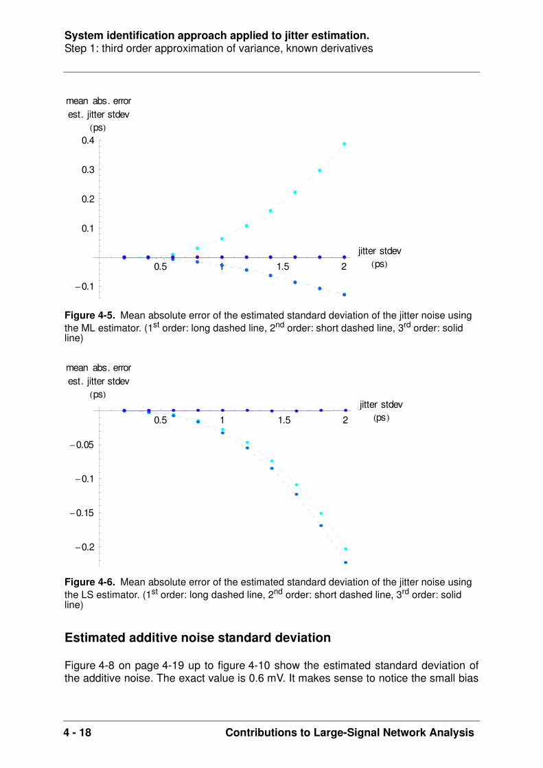
System identification approach applied to jitter estimation.Step 1: third order approximation of variance, known derivatives
4 - 18 Contributions to Large-Signal Network Analysis
Estimated additive noise standard deviation
Figure 4-8 on page 4-19 up to figure 4-10 show the estimated standard deviation ofthe additive noise. The exact value is 0.6 mV. It makes sense to notice the small bias
Figure 4-5. Mean absolute error of the estimated standard deviation of the jitter noise using the ML estimator. (1st order: long dashed line, 2nd order: short dashed line, 3rd order: solid line)
Figure 4-6. Mean absolute error of the estimated standard deviation of the jitter noise using the LS estimator. (1st order: long dashed line, 2nd order: short dashed line, 3rd order: solid line)
0.5 1 1.5 2
jitter stdevps
0.1
0.1
0.2
0.3
0.4
mean abs. errorest. jitter stdev
ps
0.5 1 1.5 2
jitter stdevps
0.2
0.15
0.1
0.05
mean abs. errorest. jitter stdev
ps

System identification approach applied to jitter estimation.Step 1: third order approximation of variance, known derivatives
Contributions to Large-Signal Network Analysis 4 - 19
present in the WLS estimate. This bias turns out to be independent of the jitter value.
The relative error of the estimated variance is empirically found to equal ,
where equals the number of degrees of freedom of the sampled - distribution,
Figure 4-7. Mean absolute error of the estimated standard deviation of the jitter noise using the WLS estimator. (1st order: long dashed line, 2nd order: short dashed line, 3rd order: solid line)
Figure 4-8. Mean estimated standard deviation of the additive noise using the ML estimator. (1st order: long dashed line, 2nd order: short dashed line, 3rd order: solid line)
0.5 1 1.5 2
jitter stdevps
0.25
0.2
0.15
0.1
0.05
mean abs. errorest. jitter stdev
ps
0.5 1 1.5 2
jitter stdevps
0.5994
0.5996
0.5998
0.6002
mean est. stdevadd. noise mV
4Ns Nw⋅------------------
Ns χ2

System identification approach applied to jitter estimation.Step 1: third order approximation of variance, known derivatives
4 - 20 Contributions to Large-Signal Network Analysis
and is the number of repeated realizations. As such equals the overall
number of degrees of freedom of the averaged data used to estimate bothparameters. During this simulation and . The corresponding
relative error is , the estimated standard deviation is
Figure 4-9. Mean estimated standard deviation of the additive noise using the LS estimator. (1st order: long dashed line, 2nd order: short dashed line, 3rd order: solid line)
Figure 4-10. Mean estimated standard deviation of the additive noise using the WLS estimator. (1st order: long dashed line, 2nd order: short dashed line, 3rd order: solid line)
0.5 1 1.5 2
jitter stdevps
0.62
0.64
0.66
0.68
0.7
0.72
mean est. stdevadd. noise mV
0.5 1 1.5 2
jitter stdevps
0.5998
0.6002
0.6004
0.6006
0.6008
mean est. stdevadd. noise mV
Nw Ns Nw⋅
Ns 100= Nw 200=
2 10 4–⋅

System identification approach applied to jitter estimation.Step 1: third order approximation of variance, known derivatives
Contributions to Large-Signal Network Analysis 4 - 21
mV. This value corresponds to the small offsetvisible for the third order model in figure 4-10.
Value of the cost function
The value of the cost function in case of a weighted least-squares deserves specialattention, because one can calculate the expected value of the cost and its 95%confidence interval. Figure 4-11 shows the cost for the first, second and third ordermodel. It clearly demonstrates the sensitivity of the cost with respect to model errors.Figure 4-12 and figure 4-13 on page 4-23 zoom into the sample mean and samplevariance of the cost when there are no model errors.
In order to obtain the expected value and the variance of the cost, one can reuse theexplanation found under “Random number generator” on page 4-15, taking intoaccount that the number of degrees of freedom is decreased by the number ofparameters ( ). During the simulation, the following values were used:
, , and . Replacing by in
Eq. 4-26, the expected value of the cost is found to be 4136. The variance of the
cost equals 8526. Based on realizations of the cost, one can calculate the
95% confidence intervals of its sample mean and sample variance using the
Figure 4-11. Mean value of the cost using the WLS estimator. (1st order: long dashed line, 2nd order: short dashed line, 3rd order: solid line)
0.6 1 2 10 4–⋅–⋅ 0.59994=
0.5 1 1.5 2
jitter stdevps
25
50
75
100
125
150
175
cost x103
p 2=Ns 100= Nt 4096= Nw 200= Ne 250= Nt Nt p–
µV
σV2
Ne
VNeSNe
2

System identification approach applied to jitter estimation.Step 1: third order approximation of variance, known derivatives
4 - 22 Contributions to Large-Signal Network Analysis
Student-t and - distribution:
Eq. 4-28
Eq. 4-29
For the actual simulation parameters, the 95% confidence intervals become:
Eq. 4-30
Eq. 4-31
The 95% confidence intervals are shown in figure 4-12 and figure 4-13.
Based on the simulation results it can be concluded that the estimated parametersconverge to the exact parameters when there are no model errors. A small biasbecomes apparent for the estimated standard deviation of the additive noise in case ofthe weighted least-squares estimator. This bias decreases as function of anincreasing number of averages1 used while estimating the standard deviation of theadditive noise.
In case of a WLS estimator, it is demonstrated that both the sample mean and samplevariance of the cost match their expected value within their 95% confidence intervalswhen there are no model errors, while there is a significant difference when there aremodel errors. This clearly shows the capability of a WLS estimator with respect tomodel selection.
1. Corresponding to a - distribution with an increasing number of degrees of freedom, as such converging to a normal distribution.
χ Ne 1–( )2
PNe 1–( ) SNe
2
χNe 1– 1 α
2---–,
2------------------------------ σV
2 Ne 1–( ) SNe
2
χNe 1– α
2---,
2-----------------------------≤ ≤
1 α–=
P VNe
SNe
Ne
---------- tNe 1– 1 α
2---–,
– µV VNe
SNe
Ne
---------- tNe 1– 1 α
2---–,
+≤ ≤
1 α–=
0.845 SNe
2 σV2
1.202 SNe
2≤ ≤
VNe1.970
SNe
2
Ne--------– µV VNe
1.970SNe
2
Ne--------+≤ ≤
χ2

System identification approach applied to jitter estimation.Step 1: third order approximation of variance, known derivatives
Contributions to Large-Signal Network Analysis 4 - 23
Figure 4-12. Expected value (dashed line) of the cost of the 3rd order model using the WLS estimator, compared to its sample mean value (250 realizations) and its 95% confidence interval.
Figure 4-13. Expected variance (dashed line) of the cost of the 3rd order model using the WLS estimator, compared to its sample variance value (250 realizations) and its 95% confidence interval.
0.5 1 1.5 2
jitter stdevps
4120
4130
4140
4150
4160
4170mean cost
0.5 1 1.5 2
jitter stdevps
7
8
9
10
11
12
variance ofcost x103

System identification approach applied to jitter estimation.Step 1: third order approximation of variance, known derivatives
4 - 24 Contributions to Large-Signal Network Analysis
Using the covariance matrix of the parameters
Finally it is verified that the uncertainty on the parameters, indicated by the parametercovariance matrix, corresponds to the sample variance of the parameters based on
repeated estimations.
In order not to clutter the figures, the 95% confidence interval of the sample varianceof the estimated variances is not shown.
For estimations, .
Figure 4-14 shows the comparison of the estimated variance of the additive noise fora third order model in combination with the WLS estimator. Figure 4-15 repeats thiscomparison for the estimated variance of the jitter noise for the same model andestimator. Finally, figure 4-16 shows that the uncertainty on the estimated jittervariance is indeed smaller using a WLS estimator instead of a (unweighted) LSestimator.
It can be concluded that the parameter covariance matrix can be used to obtain anestimate of the uncertainty on the estimated parameters. As such, one does not haveto perform repeated estimations in order to get an idea of the uncertainty on theestimated parameters.
An overview of the simulation results can be found in Table 4-1 and Table 4-2.
Figure 4-14. Variance of the estimated variance of the additive noise (solid line: based on the parameter covariance matrix, dashed line: sample variance based on 250 estimations), 3rd order model using the WLS estimator.
Ne
σ
Ne 250= 0.845 SNe
2 σ2 1.202 SNe
2≤ ≤
0.5 1 1.5 2
jitter stdevps
2.8
3.2
3.4
3.6
3.8
4
var est. var add. noisex1021 V2

System identification approach applied to jitter estimation.Step 1: third order approximation of variance, known derivatives
Contributions to Large-Signal Network Analysis 4 - 25
Figure 4-15. Variance of the estimated variance of the jitter noise (solid line: based on the parameter covariance matrix, dashed line: sample variance based on 250 estimations), 3rd order model using the WLS estimator.
Figure 4-16. Variance of the estimated variance of the jitter noise (solid line: based on the parameter covariance matrix, dashed line: sample variance based on 250 estimations), 3rd order model using the LS estimator.
0.5 1 1.5 2
jitter stdevps
0.2
0.4
0.6
0.8
1
1.2
1.4
var est. var jitter noisex1053 s2
0.5 1 1.5 2
jitter stdevps
2.5
5
7.5
10
12.5
15
17.5
var est. var jitter noisex1053 s2

System identification approach applied to jitter estimation.Step 1: third order approximation of variance, known derivatives
4 - 26 Contributions to Large-Signal Network Analysis
estimatororder of model
mean abs. err. of est.
(ps)
one sigma unc. on est.
(fs)
mean abs. err. of est.
(mV)
one sigma unc. on est.
(µV)LS 1 -0.027 1.645 0.008 0.486
2 -0.032 1.589 0.001 0.504
3 0.000 1.801 0.000 0.501
WLS 1 -0.007 0.765 0.000 0.047
2 -0.031 0.636 0.000 0.047
3 0.000 0.699 0.000 0.047
MLE 1 0.065 0.843 0.000 0.048
2 -0.026 0.633 0.000 0.048
3 0.000 0.703 0.000 0.048
Table 4-1. Summary of the simulation results in case of a 3rd order approximation of the variance and in case of known derivatives. Case of known standard deviation of additive noise
of 0.6 mV and known standard deviation of jitter noise of 1 ps.
estimatororder of model
mean abs. err. of est.
(ps)
one sigma unc. on est.
(fs)
mean abs. err. of est.
(mV)
one sigma unc. on est.
(µV)LS 1 -0.203 2.727 0.127 1.673
2 -0.223 2.400 0.043 1.748
3 0.000 3.364 0.000 1.509
WLS 1 -0.253 0.985 0.001 0.048
2 -0.244 0.760 0.000 0.048
3 0.000 0.917 0.000 0.048
MLE 1 0.388 1.414 0.000 0.049
2 -0.128 0.739 -0.001 0.049
3 0.000 0.922 0.000 0.048
Table 4-2. Summary of the simulation results in case of a 3rd order approximation of the variance and in case of known derivatives. Case of known standard deviation of additive noise
of 0.6 mV and known standard deviation of jitter noise of 2 ps.
σntσnt
σnyσny
σnyσnt
σntσnt
σnyσny
σnyσnt

System identification approach applied to jitter estimation.Step 2: realistic variance, known derivatives
Contributions to Large-Signal Network Analysis 4 - 27
Step 2: realistic variance,known derivatives
Here, the simulated sample variance is obtained based on
. Eq. 4-32
The standard deviation of the additive noise is fixed to 0.6 mV, while the
standard deviation of the jitter noise is stepped from 0 to 2 ps in 0.2 ps steps.
The required derivatives of the pulse are assumed to be known. In step 3, thederivatives will be calculated starting from the sample mean of the pulse and theestimated variance of the jitter noise. This allows to verify the impact of uncertaintieson the required derivatives.
Simulation data for the sample mean and sample variance of the pulse is obtainedusing a normal distribution for both and , and based on
100 realizations of the pulse. The sample variance of the sample variance is based on100 repeated realizations. Finally, the variance of the additive and jitter noise isestimated and this process is repeated 50 times.
Estimated jitter standard deviation
Figure 4-17 up to figure 4-19 show the sample mean of the absolute error of theestimated jitter standard deviation. It is clear that the third order model in combinationwith an unweighted LS estimator provides the best estimate for the jitter standarddeviation. The mean relative error is 0.03% for a jitter standard deviation of 1 ps, whileit is 0.3% using the WLS estimator.
Estimated additive noise standard deviation
Figure 4-20 on page 4-29 up to figure 4-22 show the estimated standard deviation ofthe additive noise. The exact value is 0.6 mV. Note that the mean relative error of afirst order model in combination with an unweighted LS estimator is 1.25% for a jitterstandard deviation of 1 ps. Using a third order model, this relative error is reduced to0.11% and using a WLS estimator this error is further reduced to 0.02%.
Value of the cost function
Again, the value of the cost function in case of a weighted least-squares deservesspecial attention. Figure 4-23 shows the cost for the first, second and third order
y ti( ) y0 ti nt ti( )+( ) ny ti( )+=
ny ti( )
nt ti( )
ny ti( ) nt ti( ) i 1 .. 4096=
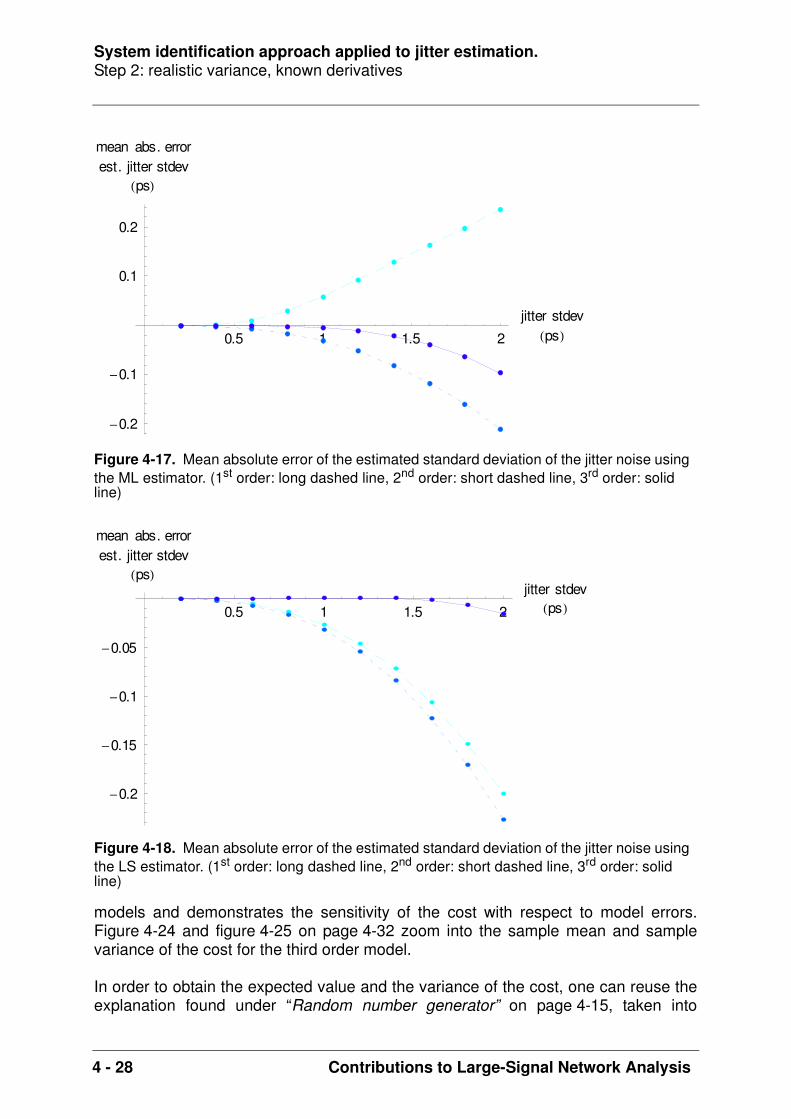
System identification approach applied to jitter estimation.Step 2: realistic variance, known derivatives
4 - 28 Contributions to Large-Signal Network Analysis
models and demonstrates the sensitivity of the cost with respect to model errors.Figure 4-24 and figure 4-25 on page 4-32 zoom into the sample mean and samplevariance of the cost for the third order model.
In order to obtain the expected value and the variance of the cost, one can reuse theexplanation found under “Random number generator” on page 4-15, taken into
Figure 4-17. Mean absolute error of the estimated standard deviation of the jitter noise using the ML estimator. (1st order: long dashed line, 2nd order: short dashed line, 3rd order: solid line)
Figure 4-18. Mean absolute error of the estimated standard deviation of the jitter noise using the LS estimator. (1st order: long dashed line, 2nd order: short dashed line, 3rd order: solid line)
0.5 1 1.5 2
jitter stdevps
0.2
0.1
0.1
0.2
mean abs. errorest. jitter stdev
ps
0.5 1 1.5 2
jitter stdevps
0.2
0.15
0.1
0.05
mean abs. errorest. jitter stdev
ps

System identification approach applied to jitter estimation.Step 2: realistic variance, known derivatives
Contributions to Large-Signal Network Analysis 4 - 29
account that the number of degrees of freedom is decreased by the number ofparameters ( ). During this simulation, the following values were used:
, , and . Replacing by in Eq.
4-26, the expected value of the cost is found to be 4178. The variance of the cost
Figure 4-19. Mean absolute error of the estimated standard deviation of the jitter noise using the WLS estimator. (1st order: long dashed line, 2nd order: short dashed line, 3rd order: solid line)
Figure 4-20. Mean estimated standard deviation of the additive noise using the ML estimator. (1st order: long dashed line, 2nd order: short dashed line, 3rd order: solid line)
0.5 1 1.5 2
jitter stdevps
0.3
0.25
0.2
0.15
0.1
0.05
mean abs. errorest. jitter stdev
ps
0.5 1 1.5 2
jitter stdevps
0.5992
0.5994
0.5996
0.5998
mean est. stdevadd. noise mV
p 2=Ns 100= Nt 4096= Nw 100= Ne 50= Nt Nt p–
µV

System identification approach applied to jitter estimation.Step 2: realistic variance, known derivatives
4 - 30 Contributions to Large-Signal Network Analysis
equals 8888. Using Eq. 4-28 and Eq. 4-29, one can calculate the 95% confidence
intervals for the expected value of the cost and its variance. These are shown infigure 4-24 and figure 4-25. For jitter standard deviations of more than 1 ps, therealized costs clearly deviate from the expected value of the cost. The asymmetry ofthe 95% confidence interval of the sample variance of the cost is due to the
Figure 4-21. Mean estimated standard deviation of the additive noise using the LS estimator. (1st order: long dashed line, 2nd order: short dashed line, 3rd order: solid line)
Figure 4-22. Mean estimated standard deviation of the additive noise using the WLS estimator. (1st order: long dashed line, 2nd order: short dashed line, 3rd order: solid line)
0.5 1 1.5 2
jitter stdevps
0.58
0.62
0.64
0.66
0.68
mean est. stdevadd. noise mV
0.5 1 1.5 2
jitter stdevps
0.5996
0.5998
0.6002
0.6004
mean est. stdevadd. noise mV
σV2
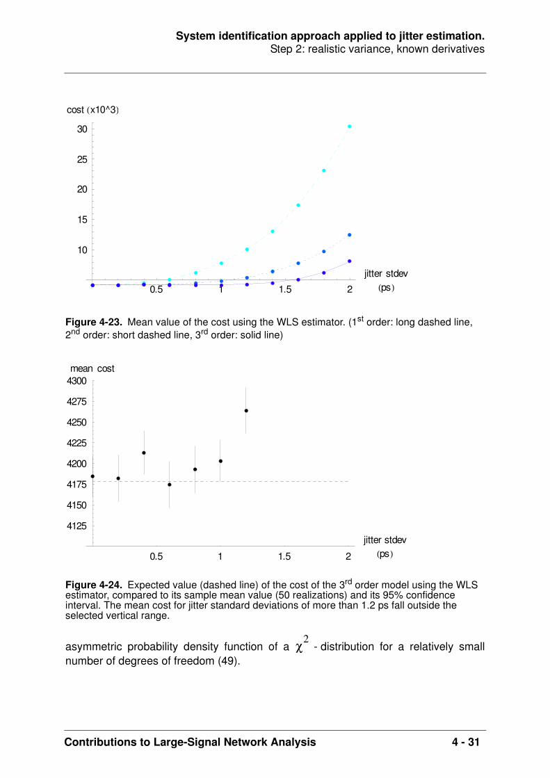
System identification approach applied to jitter estimation.Step 2: realistic variance, known derivatives
Contributions to Large-Signal Network Analysis 4 - 31
asymmetric probability density function of a - distribution for a relatively smallnumber of degrees of freedom (49).
Figure 4-23. Mean value of the cost using the WLS estimator. (1st order: long dashed line, 2nd order: short dashed line, 3rd order: solid line)
Figure 4-24. Expected value (dashed line) of the cost of the 3rd order model using the WLS estimator, compared to its sample mean value (50 realizations) and its 95% confidence interval. The mean cost for jitter standard deviations of more than 1.2 ps fall outside the selected vertical range.
0.5 1 1.5 2
jitter stdevps
10
15
20
25
30
cost x10^3
0.5 1 1.5 2
jitter stdevps
4125
4150
4175
4200
4225
4250
4275
4300mean cost
χ2
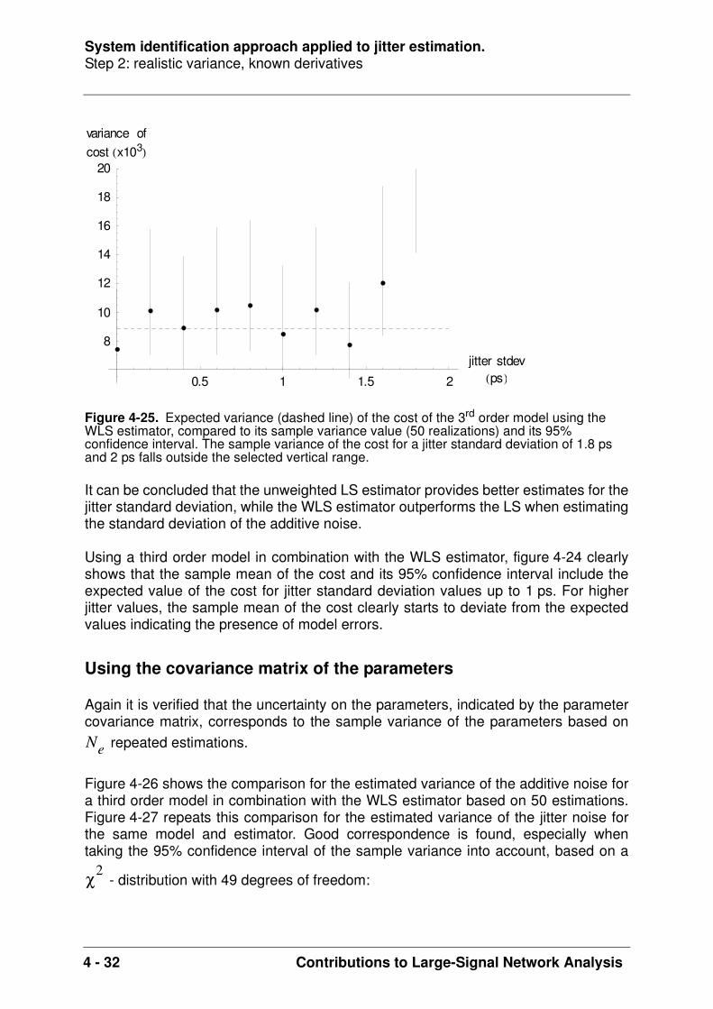
System identification approach applied to jitter estimation.Step 2: realistic variance, known derivatives
4 - 32 Contributions to Large-Signal Network Analysis
It can be concluded that the unweighted LS estimator provides better estimates for thejitter standard deviation, while the WLS estimator outperforms the LS when estimatingthe standard deviation of the additive noise.
Using a third order model in combination with the WLS estimator, figure 4-24 clearlyshows that the sample mean of the cost and its 95% confidence interval include theexpected value of the cost for jitter standard deviation values up to 1 ps. For higherjitter values, the sample mean of the cost clearly starts to deviate from the expectedvalues indicating the presence of model errors.
Using the covariance matrix of the parameters
Again it is verified that the uncertainty on the parameters, indicated by the parametercovariance matrix, corresponds to the sample variance of the parameters based on
repeated estimations.
Figure 4-26 shows the comparison for the estimated variance of the additive noise fora third order model in combination with the WLS estimator based on 50 estimations.Figure 4-27 repeats this comparison for the estimated variance of the jitter noise forthe same model and estimator. Good correspondence is found, especially whentaking the 95% confidence interval of the sample variance into account, based on a
- distribution with 49 degrees of freedom:
Figure 4-25. Expected variance (dashed line) of the cost of the 3rd order model using the WLS estimator, compared to its sample variance value (50 realizations) and its 95% confidence interval. The sample variance of the cost for a jitter standard deviation of 1.8 ps and 2 ps falls outside the selected vertical range.
0.5 1 1.5 2
jitter stdevps
8
10
12
14
16
18
20
variance ofcost x103
Ne
χ2

System identification approach applied to jitter estimation.Step 2: realistic variance, known derivatives
Contributions to Large-Signal Network Analysis 4 - 33
Eq. 4-33
Finally, figure 4-28 shows that the uncertainty on the estimated jitter variance isindeed smaller when using a WLS estimator instead of a (unweighted) LS estimator.However, the uncertainty on the estimated jitter standard deviation is sufficiently smallto prefer the LS estimator over the WLS. Indeed, starting from the sample variance ofthe sample variance, one can calculate the standard deviation on the standarddeviation:
Eq. 4-34
As such, the variance of the estimated variance of 2.5 10-53 boils down to a 95%confidence interval on the estimated jitter standard deviation of ± 5 fs in case of aknown jitter standard deviation of 1 ps.
It should be noticed that the number of pulse realizations used for one estimate of theparameters, is 104. Decreasing this number will increase the uncertainty on theparameters. Given a specified tolerance on the estimated parameters, using a smallernumber of realizations, the larger uncertainty of the LS-based estimates may becomean argument to prefer the WLS estimator over the LS estimator. Finally, one shouldrecall that the WLS estimator has the additional advantage of providing a cost which
Figure 4-26. Variance of the estimated variance of the additive noise (solid line: based on the parameter covariance matrix, dashed line: sample variance based on 50 estimations), 3rd order model using the WLS estimator.
0.5 1 1.5 2
jitter stdevps
5.5
6.5
7
7.5
8
8.5
var est. var add. noisex1021 V2
0.698 SNe
2 σV2 1.553 SNe
2≤ ≤
σx
σx2
4x------≅
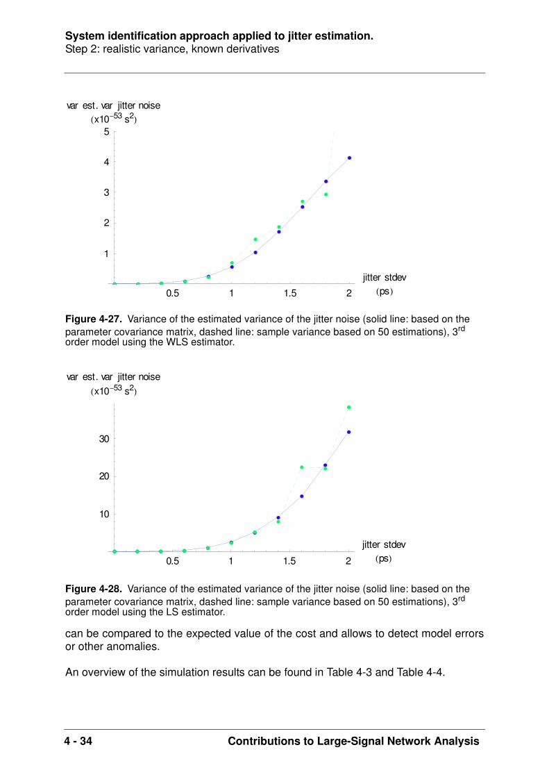
System identification approach applied to jitter estimation.Step 2: realistic variance, known derivatives
4 - 34 Contributions to Large-Signal Network Analysis
can be compared to the expected value of the cost and allows to detect model errorsor other anomalies.
An overview of the simulation results can be found in Table 4-3 and Table 4-4.
Figure 4-27. Variance of the estimated variance of the jitter noise (solid line: based on the parameter covariance matrix, dashed line: sample variance based on 50 estimations), 3rd order model using the WLS estimator.
Figure 4-28. Variance of the estimated variance of the jitter noise (solid line: based on the parameter covariance matrix, dashed line: sample variance based on 50 estimations), 3rd order model using the LS estimator.
0.5 1 1.5 2
jitter stdevps
1
2
3
4
5
var est. var jitter noisex1053 s2
0.5 1 1.5 2
jitter stdevps
10
20
30
var est. var jitter noisex1053 s2

System identification approach applied to jitter estimation.Step 2: realistic variance, known derivatives
Contributions to Large-Signal Network Analysis 4 - 35
estimatororder of model
mean abs. err. of est.
(ps)
one sigma unc. on est.
(fs)
mean abs. err. of est.
(mV)
one sigma unc. on est.
(µV)LS 1 -0.027 2.249 0.008 0.683
2 -0.032 2.175 0.000 0.701
3 0.000 2.468 -0.001 0.696
WLS 1 -0.026 1.128 0.000 0.067
2 -0.041 1.028 0.000 0.067
3 -0.003 1.183 0.000 0.067
MLE 1 0.058 1.180 0.000 0.067
2 -0.031 0.890 0.000 0.067
3 -0.005 0.987 0.000 0.067
Table 4-3. Summary of the simulation results in case of a realistic variance and in case of
known derivatives. Case of known standard deviation of additive noise of 0.6 mV and
known standard deviation of jitter noise of 1 ps.
estimatororder of model
mean abs. err. of est.
(ps)
one sigma unc. on est.
(fs)
mean abs. err. of est.
(mV)
one sigma unc. on est.
(µV)LS 1 -0.200 3.417 0.093 2.361
2 -0.227 3.064 0.014 2.286
3 -0.016 4.457 -0.017 1.957
WLS 1 -0.305 1.305 0.000 0.068
2 -0.337 1.095 0.000 0.068
3 -0.108 1.607 0.000 0.068
MLE 1 0.236 1.811 0.000 0.068
2 -0.211 0.987 -0.001 0.068
3 -0.097 1.223 0.000 0.068
Table 4-4. Summary of the simulation results in case of a realistic variance and in case of
known derivatives. Case of known standard deviation of additive noise of 0.6 mV and
known standard deviation of jitter noise of 2 ps.
σntσnt
σnyσny
σny
σnt
σntσnt
σnyσny
σny
σnt
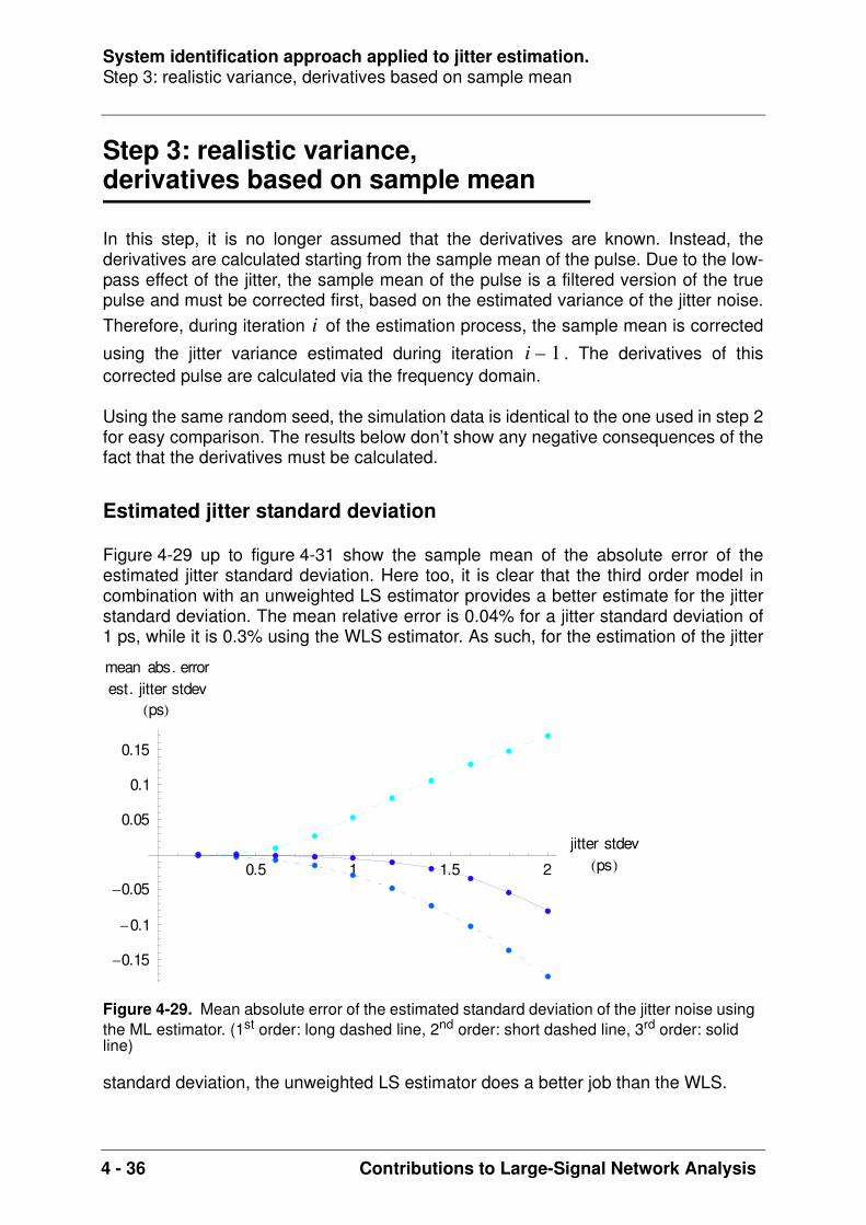
System identification approach applied to jitter estimation.Step 3: realistic variance, derivatives based on sample mean
4 - 36 Contributions to Large-Signal Network Analysis
Step 3: realistic variance,derivatives based on sample mean
In this step, it is no longer assumed that the derivatives are known. Instead, thederivatives are calculated starting from the sample mean of the pulse. Due to the low-pass effect of the jitter, the sample mean of the pulse is a filtered version of the truepulse and must be corrected first, based on the estimated variance of the jitter noise.Therefore, during iteration of the estimation process, the sample mean is corrected
using the jitter variance estimated during iteration . The derivatives of thiscorrected pulse are calculated via the frequency domain.
Using the same random seed, the simulation data is identical to the one used in step 2for easy comparison. The results below don’t show any negative consequences of thefact that the derivatives must be calculated.
Estimated jitter standard deviation
Figure 4-29 up to figure 4-31 show the sample mean of the absolute error of theestimated jitter standard deviation. Here too, it is clear that the third order model incombination with an unweighted LS estimator provides a better estimate for the jitterstandard deviation. The mean relative error is 0.04% for a jitter standard deviation of1 ps, while it is 0.3% using the WLS estimator. As such, for the estimation of the jitter
standard deviation, the unweighted LS estimator does a better job than the WLS.
Figure 4-29. Mean absolute error of the estimated standard deviation of the jitter noise using the ML estimator. (1st order: long dashed line, 2nd order: short dashed line, 3rd order: solid line)
ii 1–
0.5 1 1.5 2
jitter stdevps
0.15
0.1
0.05
0.05
0.1
0.15
mean abs. errorest. jitter stdev
ps

System identification approach applied to jitter estimation.Step 3: realistic variance, derivatives based on sample mean
Contributions to Large-Signal Network Analysis 4 - 37
Estimated additive noise standard deviation
Figure 4-32 up to figure 4-34 show the estimated standard deviation of the additivenoise. The exact value is 0.6 mV. Note that the mean relative error of a first order
Figure 4-30. Mean absolute error of the estimated standard deviation of the jitter noise using the LS estimator. (1st order: long dashed line, 2nd order: short dashed line, 3rd order: solid line)
Figure 4-31. Mean absolute error of the estimated standard deviation of the jitter noise using the WLS estimator. (1st order: long dashed line, 2nd order: short dashed line, 3rd order: solid line)
0.5 1 1.5 2
jitter stdevps
0.175
0.15
0.125
0.1
0.075
0.05
0.025
mean abs . errorest. jitter stdev
ps
0.5 1 1.5 2
jitter stdevps
0.25
0.2
0.15
0.1
0.05
mean abs. errorest. jitter stdev
ps
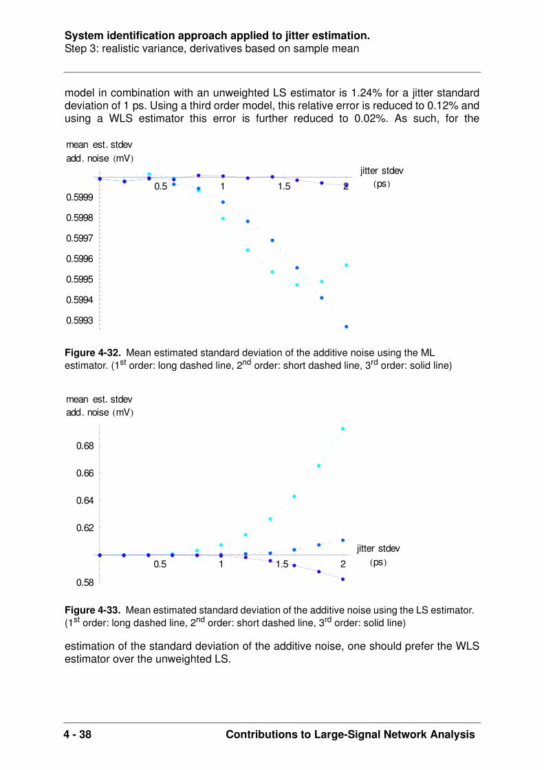
System identification approach applied to jitter estimation.Step 3: realistic variance, derivatives based on sample mean
4 - 38 Contributions to Large-Signal Network Analysis
model in combination with an unweighted LS estimator is 1.24% for a jitter standarddeviation of 1 ps. Using a third order model, this relative error is reduced to 0.12% andusing a WLS estimator this error is further reduced to 0.02%. As such, for the
estimation of the standard deviation of the additive noise, one should prefer the WLSestimator over the unweighted LS.
Figure 4-32. Mean estimated standard deviation of the additive noise using the ML estimator. (1st order: long dashed line, 2nd order: short dashed line, 3rd order: solid line)
Figure 4-33. Mean estimated standard deviation of the additive noise using the LS estimator. (1st order: long dashed line, 2nd order: short dashed line, 3rd order: solid line)
0.5 1 1.5 2
jitter stdevps
0.5993
0.5994
0.5995
0.5996
0.5997
0.5998
0.5999
mean est. stdevadd. noise mV
0.5 1 1.5 2
jitter stdevps
0.58
0.62
0.64
0.66
0.68
mean est. stdevadd. noise mV

System identification approach applied to jitter estimation.Step 3: realistic variance, derivatives based on sample mean
Contributions to Large-Signal Network Analysis 4 - 39
Value of the cost function
Figure 4-35 shows the mean cost for the first, second and third order model incombination with a WLS estimator. Figure 4-36 and figure 4-37 zoom into the samplemean and sample variance of the cost for the third order model.
Figure 4-34. Mean estimated standard deviation of the additive noise using the WLS estimator. (1st order: long dashed line, 2nd order: short dashed line, 3rd order: solid line)
Figure 4-35. Mean value of the cost using the WLS estimator. (1st order: long dashed line, 2nd order: short dashed line, 3rd order: solid line)
0.5 1 1.5 2
jitter stdevps
0.5998
0.6002
0.6004
mean est. stdevadd. noise mV
0.5 1 1.5 2
jitter stdevps
10
15
20
25
cost x103

System identification approach applied to jitter estimation.Step 3: realistic variance, derivatives based on sample mean
4 - 40 Contributions to Large-Signal Network Analysis
The expected value of the cost, , its variance and their 95% confidence
interval equal those of step 2. These are shown in figure 4-36 and figure 4-37.
Figure 4-36. Expected value (dashed line) of the cost of the 3rd order model using the WLS estimator, compared to its sample mean value (50 realizations) and its 95% confidence interval. The mean cost for jitter standard deviations of more than 1.2 ps fall outside the selected vertical range.
Figure 4-37. Expected variance (dashed line) of the cost of the 3rd order model using the WLS estimator, compared to its sample variance value (50 realizations) and its 95% confidence interval. The sample variance of the cost for a jitter standard deviation of 1.8 ps and 2 ps falls outside the selected vertical range.
0.5 1 1.5 2
jitter stdevps
4125
4150
4175
4200
4225
4250
4275
4300mean cost
0.5 1 1.5 2
jitter stdevps
8
10
12
14
16
18
20
variance ofcost x103
µV σV2

System identification approach applied to jitter estimation.Step 3: realistic variance, derivatives based on sample mean
Contributions to Large-Signal Network Analysis 4 - 41
Comparing figure 4-24 to figure 4-36 and figure 4-25 to figure 4-37, it is clear that theeffect of not knowing the exact derivatives is negligible. As was the case in step 2, thecost starts deviating from the expected cost for jitter values larger than 1 ps, implyingthe presence of model errors.
Using the covariance matrix of the parameters
Again, the uncertainty on the parameters obtained from theory and simulation arecompared. It is verified if the uncertainty on the parameters, indicated by theparameter covariance matrix, corresponds to the sample variance of the parametersbased on repeated estimations.
Figure 4-38 shows the comparison for the estimated variance of the additive noise fora third order model in combination with the WLS estimator based on 50 estimations.Again, good correspondence is found after taking the 95% confidence interval of the
sample variance into account, based on a - distribution with 49 degrees offreedom (Eq. 4-33). Figure 4-39 repeats this comparison for the estimated variance ofthe jitter noise for the same model and estimator. Finally, figure 4-40 shows that oncemore the uncertainty on the estimated jitter variance is smaller using a WLS estimatorinstead of a (unweighted) LS estimator. Again, the uncertainty on the estimated jitterstandard deviation is similar to that of step 2 and as such sufficiently small to preferthe LS estimator over the WLS for the estimation of the jitter standard deviation, whilethe WLS is preferred over the LS estimator when estimating the standard deviation ofthe additive noise.
Figure 4-38. Variance of the estimated variance of the additive noise (solid line: based on the parameter covariance matrix, dashed line: sample variance based on 50 estimations), 3rd order model using the WLS estimator.
Ne
0.5 1 1.5 2
jitter stdevps
5.5
6.5
7
7.5
8
8.5
var est. var add. noisex1021 V2
χ2

System identification approach applied to jitter estimation.Step 3: realistic variance, derivatives based on sample mean
4 - 42 Contributions to Large-Signal Network Analysis
An overview of the simulation results can be found in Table 4-5 and Table 4-6.
Figure 4-39. Variance of the estimated variance of the jitter noise (solid line: based on the parameter covariance matrix, dashed line: sample variance based on 50 estimations), 3rd order model using the WLS estimator.
Figure 4-40. Variance of the estimated variance of the jitter noise (solid line: based on the parameter covariance matrix, dashed line: sample variance based on 50 estimations), 3rd order model using the LS estimator.
0.5 1 1.5 2
jitter stdevps
1
2
3
4
5
var est. var jitter noisex1053 s2
0.5 1 1.5 2
jitter stdevps
10
20
30
40
var est. var jitter noisex1053 s2

System identification approach applied to jitter estimation.Step 3: realistic variance, derivatives based on sample mean
Contributions to Large-Signal Network Analysis 4 - 43
estimatororder of model
mean abs. err. of est.
(ps)
one sigma unc. on est.
(fs)
mean abs. err. of est.
(mV)
one sigma unc. on est.
(µV)LS 1 -0.025 2.257 0.007 0.682
2 -0.030 2.184 0.000 0.701
3 0.000 2.468 -0.001 0.696
WLS 1 -0.024 1.133 0.000 0.067
2 -0.038 1.034 0.000 0.067
3 -0.003 1.184 0.000 0.067
MLE 1 0.053 1.173 0.000 0.068
2 -0.029 0.898 0.000 0.068
3 -0.005 0.993 0.000 0.068
Table 4-5. Summary of the simulation results in case of a realistic variance and in case of derivatives based on the sample mean. Case of known standard deviation of additive noise
of 0.6 mV and known standard deviation of jitter noise of 1 ps.
estimatororder of model
mean abs. err. of est.
(ps)
one sigma unc. on est.
(fs)
mean abs. err. of est.
(mV)
one sigma unc. on est.
(µV)LS 1 -0.161 3.564 0.093 2.351
2 -0.185 3.199 0.011 2.270
3 -0.012 4.474 -0.018 1.954
WLS 1 -0.219 1.435 0.000 0.068
2 -0.250 1.195 0.000 0.068
3 -0.082 1.646 0.000 0.068
MLE 1 0.170 1.700 0.000 0.069
2 -0.173 1.047 -0.001 0.069
3 -0.080 1.257 0.000 0.069
Table 4-6. Summary of the simulation results in case of a realistic variance and in case of derivatives based on the sample mean. Case of known standard deviation of additive noise
of 0.6 mV and known standard deviation of jitter noise of 2 ps.
σntσnt
σnyσny
σnyσnt
σntσnt
σnyσny
σnyσnt
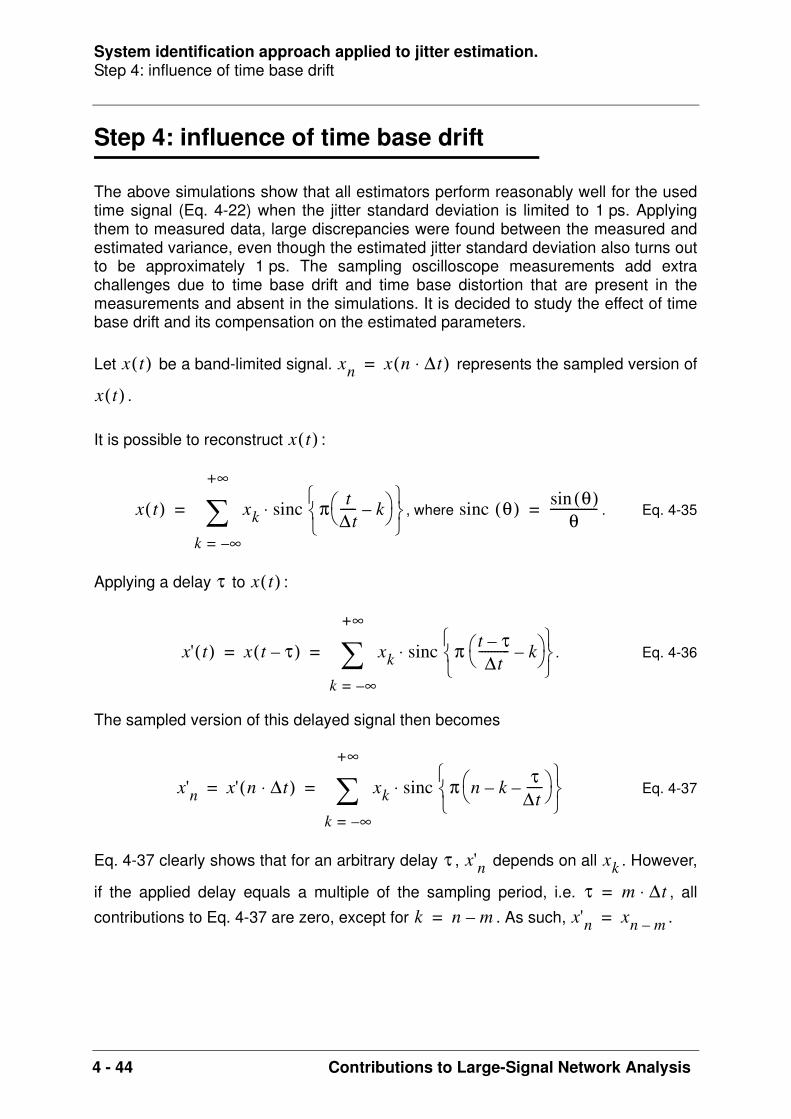
System identification approach applied to jitter estimation.Step 4: influence of time base drift
4 - 44 Contributions to Large-Signal Network Analysis
Step 4: influence of time base drift
The above simulations show that all estimators perform reasonably well for the usedtime signal (Eq. 4-22) when the jitter standard deviation is limited to 1 ps. Applyingthem to measured data, large discrepancies were found between the measured andestimated variance, even though the estimated jitter standard deviation also turns outto be approximately 1 ps. The sampling oscilloscope measurements add extrachallenges due to time base drift and time base distortion that are present in themeasurements and absent in the simulations. It is decided to study the effect of timebase drift and its compensation on the estimated parameters.
Let be a band-limited signal. represents the sampled version of
.
It is possible to reconstruct :
, where . Eq. 4-35
Applying a delay to :
. Eq. 4-36
The sampled version of this delayed signal then becomes
Eq. 4-37
Eq. 4-37 clearly shows that for an arbitrary delay , depends on all . However,
if the applied delay equals a multiple of the sampling period, i.e. , all
contributions to Eq. 4-37 are zero, except for . As such, .
x t( ) xn x n ∆t⋅( )=
x t( )
x t( )
x t( ) xk sinc π t∆t----- k–
⋅
k ∞–=
+∞
= sinc θ( ) θ( )sinθ
---------------=
τ x t( )
x' t( ) x t τ–( ) xk sinc π t τ–∆t
---------- k–
⋅
k ∞–=
+∞
= =
x'n x' n ∆t⋅( ) xk sinc π n k τ∆t-----––
⋅
k ∞–=
+∞
= =
τ x'n xk
τ m ∆t⋅=k n m–= x'n xn m–=

System identification approach applied to jitter estimation.Step 4: influence of time base drift
Contributions to Large-Signal Network Analysis 4 - 45
Based on the above, it is clear that, starting from a time sequence , , of
independent stochastical variables with known variance , the variance of the
sampled version of the arbitrarily delayed signal equals
. Moreover, is no longer independent with respect to .
Applying the same delay to the original variance , .
Obviously for a general sequence .
If the applied delay is an integer multiple of the sampling period, i.e. , then
. In that case .
The analytical pulse (Eq. 4-22) is used to study the shaping of the variance as function
of . First a known delay , , is applied to the
analytical expression. The sample variance of this delayed pulse is obtained based on1000 realizations using a standard deviation of 0.6 mV of the additive noise and astandard deviation of 1 ps of the jitter noise. Next the inverse delay is applied to thissample variance and compared to the sample variance of the original pulse( ).
Figure 4-41 clearly indicates that the shaping of the sample variance is very limitedwhen the delay is limited to .
However, when a delay is applied of , the effect is significant.
Especially the increased level of the minima of the sample variance, corresponding toa zero slope of the average pulse, incorrectly amplifies the observation that the firstorder approximation of the model equation (Eq. 4-3) no longer holds.
xn n 1 .. = N
σn2
x'n ak xk⋅
k 1=
N
=
σ'n2
ak2 σk
2⋅
k 1=
N
= x'n n
σn2 σn
2ak σk
2⋅
k 1=
N
=
σ'n2 σn
2≠ ak
τ m ∆t⋅=
x'n xn m–= σ'n2 σn
2=
τ∆t----- τ k ∆t
10------⋅= k 1 .. 5= ∆t 5 ns
4096------------=
∆t 0=
0.1∆t
0.5∆t
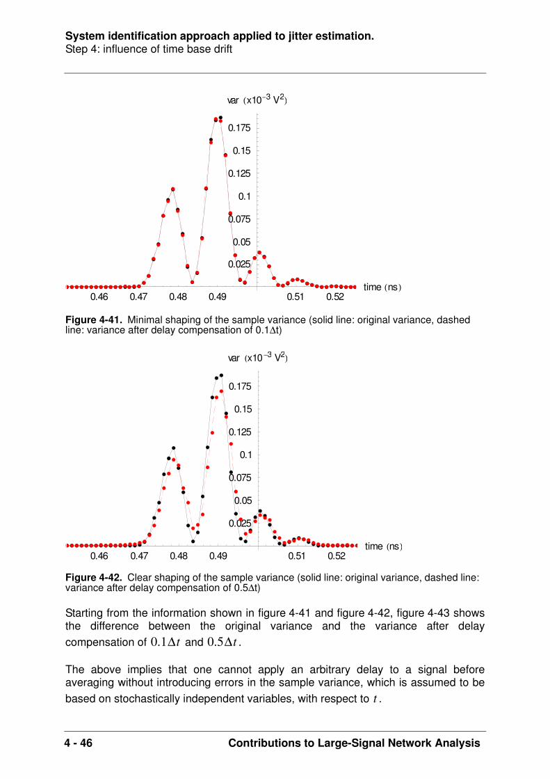
System identification approach applied to jitter estimation.Step 4: influence of time base drift
4 - 46 Contributions to Large-Signal Network Analysis
Starting from the information shown in figure 4-41 and figure 4-42, figure 4-43 showsthe difference between the original variance and the variance after delaycompensation of and .
The above implies that one cannot apply an arbitrary delay to a signal beforeaveraging without introducing errors in the sample variance, which is assumed to bebased on stochastically independent variables, with respect to .
Figure 4-41. Minimal shaping of the sample variance (solid line: original variance, dashed line: variance after delay compensation of 0.1∆t)
Figure 4-42. Clear shaping of the sample variance (solid line: original variance, dashed line: variance after delay compensation of 0.5∆t)
0.46 0.47 0.48 0.49 0.51 0.52time ns
0.025
0.05
0.075
0.1
0.125
0.15
0.175
var x103 V2
0.46 0.47 0.48 0.49 0.51 0.52time ns
0.025
0.05
0.075
0.1
0.125
0.15
0.175
var x103 V2
0.1∆t 0.5∆t
t

System identification approach applied to jitter estimation.Step 4: influence of time base drift
Contributions to Large-Signal Network Analysis 4 - 47
According to figure 4-4 on page 4-14, which shows the sample variance of impulseresponse measurements after time base drift compensation, the measurement indeedsuffers from the above error. Using this sample variance, the estimated time base jitteris incorrect.
A similar problem becomes apparent when compensating for the time base distortion.Any interpolation combines two or more values of the non-equidistant time grid toobtain an estimate of the value at the equidistant time grid points. This again shapesthe variance and introduces correlation between successive time points.
The error introduced by time base drift compensation before averaging can be limitedbased on the observations that
• applying a delay which is an integer multiple of the sampling period introduces no error,• for the impulse response of interest, the shaping of the variance and as such the error is very small1 when the delay is limited to .
Therefore, the different realizations of the pulse are first delayed by integer multiplesof such that all realizations are aligned within .
Then all realizations are divided into time buckets which are wide, resulting ina 5-times oversampled signal as compared to the original signal.
Figure 4-43. Difference between the original variance and the one after delay compensation (solid line: delay of 0.1∆t, dashed line: delay of 0.5∆t)
1. The RMS value of the difference is 1.6% of the RMS value of the original variance, while the maximum value of the difference is 2.1% of the maximum value of the original variance.
0.46 0.47 0.48 0.49 0.51 0.52time ns
0.03
0.02
0.01
0.01
0.02
0.03
0.04var x103 V2
∆t
0.1∆t
∆t 0.5∆t±
0.1∆t±

System identification approach applied to jitter estimation.Step 4: influence of time base drift
4 - 48 Contributions to Large-Signal Network Analysis
Depending on the shape of the time base drift, in general the buckets will not beequally filled. As such, the uncertainty on the sample variance will vary as function ofthe bucket index. This is not an issue when using a weighted least squares to extractthe model parameters.
Time base jitter interpretable as time base drift
In case of measurements, the time base drift of each acquisition with respect to thefirst one is estimated by minimizing
Eq. 4-38
within the bandwidth of the signal .
It is impossible to fully separate time base drift and time base jitter, because the lattercan be interpreted as time base drift as shown by the following simulation. Theanalytical pulse is distorted by additive noise (0.6 mV standard deviation) and jitternoise (1 ps standard deviation). 500 realizations of 4096 points each are generated.
First the drift - which is known to be zero - is estimated using the first realization asreference signal. Next, the drift of each realization with respect to any other one isestimated in order to obtain an enhanced drift estimate with respect to the firstrealization, as advised in [8]. Figure 4-44 shows no noticeable difference betweenboth approaches.
The sample standard deviation of the estimated drift, in the case of a jitter standarddeviation of 1 ps and based on the 500 realizations, equals 0.26 ps (0.25 ps for theenhanced estimate).
Given the above and based on reasonable time constants1 corresponding to thermaleffects, it makes sense to apply smoothing to the estimated time base drift. This willaverage out the effect of the fast jitter, while it will leave the slow drift mainlyunaffected. Additional motivation for this smoothing can be found in the chapter ondrift estimation in the presence of both jitter and additive noise.
1. Assumptions with respect to time constants are explained in step 5.
V Xref ωi( ) ejωiτ–
X ωi( )⋅–2
i 1=
N
=
X ωi( )

System identification approach applied to jitter estimation.Step 4: influence of time base drift
Contributions to Large-Signal Network Analysis 4 - 49
Figure 4-44. Time base jitter interpreted as time base drift (full line: “naive” estimate, dots: enhanced estimate).
100 200 300 400 500
realizationindex
0.5
0.25
0.25
0.5
0.75
estimateddrift ps

System identification approach applied to jitter estimation.Step 5: measurements
4 - 50 Contributions to Large-Signal Network Analysis
Step 5: measurements
The measurement data correspond to the combined impulse response of an opto-electrical converter and a 50 GHz sampling oscilloscope (see figure 4-1 on page 4-12). The impulse response measurement and the required time base distortionmeasurements were performed by Tracy Clement at NIST. This contribution isgratefully acknowledged.
A time record of 5 ns was used starting at 143 ns delay and 5000 records of4096 points were acquired.
Time base drift estimation
The drift is estimated, using the first measurement as reference. Based on the factthat simulations confirmed that time base jitter may incorrectly be interpreted as timebase drift (see above) and based on reasonable time constants corresponding tothermal effects, the estimated drift is smoothed.
The thermal time constant of the sampling oscilloscope is assumed to be of the orderof minutes. The collection and storage of 5000 records of 4096 points is found to take32 minutes. As such, approximately 150 records are collected per minute. Also,practical experience shows that the shape of the time base drift strongly depends onthe environment, both with respect to temperature variations and airflow.
The smoothing can either be done using a global model such as a low-orderpolynomial or by applying a local model such as a moving average window. The latterhas the disadvantage that some realizations at both edges cannot be used, becauseno moving average exists for these realizations.
Figure 4-45 shows the estimated time base drift and its smoothed version using a4th order polynomial. The residue (figure 4-46) has a standard deviation of 0.30 psand as such approximates the 0.26 ps found earlier1 based on a jitter standarddeviation of 1 ps.
Figure 4-47 shows the equivalent when using a moving average window, which is101 realizations wide. The standard deviation of the residue (figure 4-48) is slightlysmaller: 0.28 ps.
It is unclear which smoothing method is to be preferred. It looks like themeasurements at NIST were performed under very good conditions with respect totemperature variations and airflow. Given the disadvantage of the moving averagewith respect to the loss of measurements, the smoothing based on the 4th order
1. see end of step 4 on page 4-48.
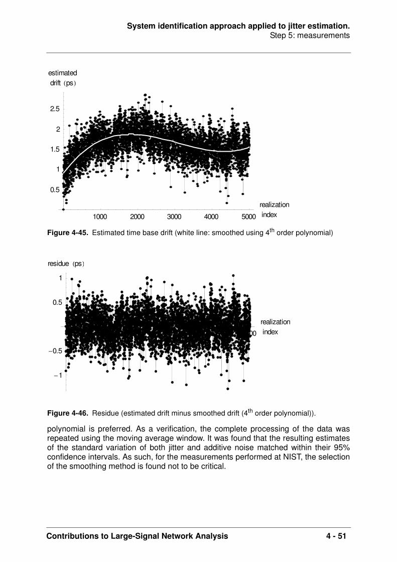
System identification approach applied to jitter estimation.Step 5: measurements
Contributions to Large-Signal Network Analysis 4 - 51
polynomial is preferred. As a verification, the complete processing of the data wasrepeated using the moving average window. It was found that the resulting estimatesof the standard variation of both jitter and additive noise matched within their 95%confidence intervals. As such, for the measurements performed at NIST, the selectionof the smoothing method is found not to be critical.
Figure 4-45. Estimated time base drift (white line: smoothed using 4th order polynomial)
Figure 4-46. Residue (estimated drift minus smoothed drift (4th order polynomial)).
1000 2000 3000 4000 5000
realizationindex
0.5
1
1.5
2
2.5
estimateddrift ps
1000 2000 3000 4000 5000
realizationindex
1
0.5
0.5
1
residue ps

System identification approach applied to jitter estimation.Step 5: measurements
4 - 52 Contributions to Large-Signal Network Analysis
Time base drift compensation
The smoothing, based on the 4th order polynomial, is used to align the differentrealizations. First all realizations are aligned within , as shown in figure 4-49.This does not introduce any shaping of the variance, as only shifts over an integernumber of samples are used.
Figure 4-47. Estimated time base drift (white line: smoothed using moving average)
Figure 4-48. Residue (estimated drift minus smoothed drift (moving average)).
1000 2000 3000 4000 5000
realizationindex
0.5
1
1.5
2
2.5
estimateddrift ps
1000 2000 3000 4000 5000
realizationindex
1
0.5
0.5
residue ps
0.5∆t±

System identification approach applied to jitter estimation.Step 5: measurements
Contributions to Large-Signal Network Analysis 4 - 53
Next, the realizations are divided in 5 buckets, each being wide. Allrealizations within each bucket are aligned with respect to the center of that bucket.Given a maximum delay of , the resulting shaping of the variance that isintroduced by the alignment can be neglected.
Figure 4-50 shows the unequal distribution of the 5000 realizations over the differentbuckets.
Figure 4-49. Drift compensated within ± 0.5 ∆t.
Figure 4-50. Distribution of the 5000 realizations over the different buckets.
1000 2000 3000 4000 5000
realizationindex
0.6
0.4
0.2
0.2
0.4
0.6
drift ps
0.1∆t±
0.1∆t
0.488 0.244 0. 0.244 0.488time ps
500
1000
1500
2000
# realizationsper bucket
879
169254
2000
1698
System identification approach applied to jitter estimation.Step 5: measurements
4 - 54 Contributions to Large-Signal Network Analysis
In order to obtain variance information, required by the WLS estimator, the realizationsper bucket must be divided into different data sets. The effect of using the samplevariance, instead of the exact variance, on the expected value and variance of thecost and on the uncertainty of the parameters as function of the number of the datasets, is studied in [6].
In order to minimize the increase of these parameters, the number of the data setsshould be sufficiently large. On the other hand, the number of realizations within each
data set should be sufficiently large too, because of the - distribution of the
sample variance, representing the number of realizations of the pulse used to
calculate the sample variance. This distribution approaches a normal distribution(assumed by [6]), only if is sufficiently large.
A possible compromise is to use a square root law. Based on the smallest number ofrealizations per bucket, as indicated in figure 4-50, both the number of data sets and
the number of realizations per data set is set to .
Another possible criterion is the allowed increase of the uncertainty of the parameters.In order to limit this increase to 10%, the number of data sets must at least be 25
( ). The corresponding increase of the expected value of the cost is
also smaller than 10%, while the uncertainty on the cost increases by less than 20%.
The jitter was estimated using two different number of data sets, i.e. 13 and 25, basedon the above mentioned criteria.
Figure 4-51 shows the sample mean of both the sample mean and sample variance ofthe 5 times oversampled pulse, each based on 25 data sets. Depending on the bucketindex, the number of realizations per data set varies from 6 to 80. As such theuncertainty on the sample variance becomes a function of the bucket index.
Time base distortion estimation and compensation
Due to the time base distortion of the Agilent 83480A Digital Communication Analyzer,the sample mean and the sample variance are specified on a non-equidistant timegrid.
The actual time jitter estimation algorithm does not require the sample mean andsample variance to be specified on an equidistant time grid. However, in order toefficiently calculate the derivatives of the mean pulse via the frequency domain usingan FFT, cubic interpolation is used to obtain the values of the sample mean on an
χNs 1–2
Ns
Ns
169 13=
Nw
Nw 1–
Nw 5–---------------- 1.1≤

System identification approach applied to jitter estimation.Step 5: measurements
Contributions to Large-Signal Network Analysis 4 - 55
equidistant grid, as proposed in [9]. Finally, the derivatives are obtained at the originalnon-equidistant grid, again by applying the “inverse” cubic interpolation. As a result,some of the points at both edges of the time record may be lost when extrapolation isnot allowed.
The time base distortion is estimated first, using [10], after collecting the required dataand making sure that both the trigger rate and time base settings are identical to thoseused during the combined impulse response measurement of the opto-electricalconverter and the sampling oscilloscope.
Figure 4-51. Sample mean of sample mean and sample variance of the oversampled pulse, each based on 25 data sets.
0.46 0.48 0.5 0.52 0.54 0.56time ns
20
20
40
60
80
mean mV
0.46 0.48 0.5 0.52 0.54 0.56time ns
0.05
0.1
0.15
0.2
var x103 V2

System identification approach applied to jitter estimation.Step 5: measurements
4 - 56 Contributions to Large-Signal Network Analysis
Figure 4-52 shows the estimated time base distortion, defined as, the non-equidistant time stamps being represented by .
For an ideal time base, all values equal zero. The lower plot zooms into theportion of the time base where the main portion of the pulse is located. All points,contributing to the main pulse, are approximately shifted 0.6 ps to the left with respectto the ideal time base. Therefore their relative distance with respect to each other isvery close to . As such it can be concluded that in this case the influence of the
Figure 4-52. Estimated time base distortion (lower plot = zoom into main portion of pulse + 95% confidence interval).
1 2 3 4 5time ns
3
2
1
1
2
estimatedTBDn ps
0.46 0.48 0.5 0.52 0.54 0.56time ns
3
2
1
1
2
estimatedTBDn ps
TBDn i[ ] ti i ∆t⋅–= tiTBDn i[ ]
∆t
System identification approach applied to jitter estimation.Step 5: measurements
Contributions to Large-Signal Network Analysis 4 - 57
time base distortion is minimal, because the main portion of the pulse does not sufferfrom any significant time base distortion, it is only shifted over a constant delay.
Applying cubic interpolation to both sample mean and sample variance , is
statistically incorrect. Indeed, the implemented cubic interpolation uses a linearcombination of the four surrounding non-equidistant points to calculate the value atthe equidistant grid:
Eq. 4-39
The correct corresponding variance equals
Eq. 4-40
Using the first order approximation to describe the variance (Eq. 4-3), the variance
on the equidistant grid becomes
. Eq. 4-41
This still requires to calculate the derivatives at the non-equidistant grid. As such it iseasier to remain on the non-equidistant grid.
Time base jitter estimation
Finally, the time base jitter can be estimated using the proposed model (Eq. 4-6) and aweighted least squares estimator, taking the varying variance of the sample varianceas function of the bucket index into account, in order to minimize the uncertainty onthe estimated parameters.
Another advantage of the weighted least squares is the fact that one is able tocalculate the expected value of the cost and its 95% confidence interval as a mean toverify the presence of model errors or other anomalies.
yi σti
2
yk∆t ai yi⋅
i 1=
4
=
σk∆t2
ai2 σti
2⋅
i 1=
4
ai σti
2⋅
i 1=
4
≠=
σti
2
σy2 k ∆t⋅( ) ai
2 σny
2⋅
i 1=
4
ai2
td
dy0
2
t ti=
σnt
2⋅ ⋅
i 1=
4
+=

System identification approach applied to jitter estimation.Step 5: measurements
4 - 58 Contributions to Large-Signal Network Analysis
Figure 4-53 shows the correctly aligned “measured” variance on a logarithmic verticalscale. It clearly shows the increased variance due to jitter corresponding to the mainpulse and to the reflection about 0.8 ps after the main pulse.
Given 25 data sets, 4096 time points1 and 2 parameters, the expected value of thecost and its 95% confidence interval equals 22324 ± 474. The actual value of the costfunction for a third order model is found to be 23582. Its value is less than 6% largerthan the expected value of the cost and slightly outside the 95% confidence interval.With respect to the first order model, the cost is decreased by more than 13%.
The estimated variance of the additive noise equals (0.258 10-6 ± 0.163 10-9) V2 andthat of the jitter noise is (0.923 10-24 ± 4.99 10-27) s2. The uncertainties correspond tothe 95% confidence interval.
The corresponding standard deviation values for the additive and jitter noise and their95% confidence intervals are 0.508 mV ± 0.16 µV and 0.961 ps ± 2.6 fs.
It is time to compare the modelled variance to the measured variance and its 95%confidence interval based on the sample variance of the measured variance. Whilefigure 4-54 zooms into the main pulse, figure 4-55 demonstrates an equally excellentfit for the first reflection. Figure 4-56 and figure 4-57 show the variance at both edgesof the record and demonstrate that also the additive noise portion fits exceptionallywell. Finally, figure 4-58 zooms into the maximum value of the variance to show the
Figure 4-53. Correctly aligned “measured” variance (logarithmic vertical scale).
1. The actual number of time points turns out to be 20466, based on the oversampling by a factor 5 and the loss of 14 points at both edges based on the cubic interpolation followed by an inverse cubic interpolation to obtain the derivatives.
1 2 3 4 5time ns
6.5
6
5.5
5
4.5
4
3.5log10var V2

System identification approach applied to jitter estimation.Step 5: measurements
Contributions to Large-Signal Network Analysis 4 - 59
uncertainty of the estimated variance as a result of the uncertainty on the estimatedparameters.
Figure 4-54. Comparing (the boundaries of the 95% confidence interval of) the (3rd order model, WLS estimator) modelled variance (red lines) and the correctly aligned “measured” variance at the main pulse (black dots and vertical black lines, boundaries of the 95% confidence intervals based on the sample variance of the sample variance).
Figure 4-55. Comparing (the boundaries of the 95% confidence interval of) the (3rd order model, WLS estimator) modelled variance (red lines) and the correctly aligned “measured” variance at the first reflection (black dots and vertical black lines, boundaries of the 95% confidence intervals based on the sample variance of the sample variance).
0.49 0.5 0.51 0.52time ns
0.05
0.1
0.15
0.2
0.25
var x103 V2
1.3 1.31 1.32 1.33time ns
0.25
0.5
0.75
1
1.25
1.5
1.75var x106 V2
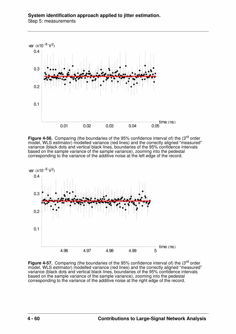
System identification approach applied to jitter estimation.Step 5: measurements
4 - 60 Contributions to Large-Signal Network Analysis
Figure 4-56. Comparing (the boundaries of the 95% confidence interval of) the (3rd order model, WLS estimator) modelled variance (red lines) and the correctly aligned “measured” variance (black dots and vertical black lines, boundaries of the 95% confidence intervals based on the sample variance of the sample variance), zooming into the pedestal corresponding to the variance of the additive noise at the left edge of the record.
Figure 4-57. Comparing (the boundaries of the 95% confidence interval of) the (3rd order model, WLS estimator) modelled variance (red lines) and the correctly aligned “measured” variance (black dots and vertical black lines, boundaries of the 95% confidence intervals based on the sample variance of the sample variance), zooming into the pedestal corresponding to the variance of the additive noise at the right edge of the record.
0.01 0.02 0.03 0.04 0.05time ns
0.1
0.2
0.3
0.4var x106 V2
4.96 4.97 4.98 4.99 5time ns
0.1
0.2
0.3
0.4var x106 V2

System identification approach applied to jitter estimation.Step 5: measurements
Contributions to Large-Signal Network Analysis 4 - 61
The correlation coefficient between the estimated variance of additive and jitter noiseturns out to be -0.12. As such there is no statistical evidence of a significantcorrelation between both estimated parameters.
Repeating the estimation based on 13 data sets, the standard deviation of the additiveand jitter noise and their 95% confidence intervals are 0.508 mV ± 0.15 µV and0.962 ps ± 2.5 fs. As such, selecting a different number of data sets has no effect onthe final estimate. The expected and realized value of the cost and its variancehowever did change, according to [6]. The realized cost turns out to be 25597, 4%above the expected value of the cost and slightly outside the 95% interval:24557 ± 583.
The power of a solid stochastical framework
It is shown that, using a solid stochastical framework, one is able to detect anomalieslike overlooking the shaping of the variance due to drift compensation. This is similarto the power demonstrated by [10] to capture anomalies with respect to the time basedistortion: due to the fact that the realized cost was significantly larger than theexpected value of the cost, it was found that, for that particular setup, the time basedistortion varied with the applied calibration frequency, while the model assumes thatthis time base distortion is identical for all applied calibration frequencies.
Suppose the shaping of the variance due to time base drift compensation isoverlooked. Repeating the above estimation procedure, using 70 data sets accordingto the “square root” rule starting from 5000 realizations, but not using any
Figure 4-58. Comparing the boundaries of the 95% confidence interval of the (3rd order model, WLS estimator) modelled variance (red lines) and the correctly aligned “measured” variance (black dots and vertical black lines, boundaries of the 95% confidence intervals based on the sample variance of the sample variance), zooming into the maximum value.
0.5 0.501 0.502 0.503 0.504 0.505time ns
0.16
0.18
0.2
0.22
var x103 V2

System identification approach applied to jitter estimation.Step 5: measurements
4 - 62 Contributions to Large-Signal Network Analysis
oversampling to limit the drift compensation to , the expected value of the costand its 95% confidence interval equals 4212 ± 188. The realized cost using a thirdorder model turns out to be 14764, which is 3.5 times the expected value of the cost.As can be seen in figure 4-59, this is confirmed by a poor correspondence betweenthe model and the variance based on incorrectly processed measurements.
Using the knowledge of the - distribution of the variance of the sample variance ofthe pulse, one can avoid the calculation of the sample variance of the sample varianceand as such reduce the number of required measurements. Figure 4-60 compares themodelled variance to the measured variance and its 95% confidence interval based
on a - distribution. The value of the cost function turns out to be 7% larger than theexpected value of the cost and is located slightly outside the 95% confidence intervalof the expected value of the cost. The standard deviation of the estimated additive andjitter noise and their 95% confidence intervals are 0.508 mV ± 0.16 µV and0.965 ps ± 2.3 fs and these match the values, obtained by using the sample varianceof the sample variance.
ML estimation
Based on Eq. 4-19, the MLE implementation can take care of the unequal distributionof the 5000 realizations over the different buckets. The corresponding varyinguncertainty is taken into account by using the appropriate number of degrees offreedom as function of the bucket index.
Figure 4-59. Comparing the (3rd order model, WLS estimator) modelled variance (connected red dots) and the incorrectly shaped “measured” variance (black dots and vertical black lines, boundaries of the 95% confidence intervals based on the sample variance of the sample variance).
0.1∆t±
0.49 0.5 0.51 0.52time ns
0.05
0.1
0.15
0.2
var x103 V2
χ2
χ2

System identification approach applied to jitter estimation.Step 5: measurements
Contributions to Large-Signal Network Analysis 4 - 63
Based on a third order model, the estimated jitter standard deviation is found to be0.970 ps ± 2.3 fs, while the estimated standard deviation of the additive noise is foundto be 0.509 mV ± 0.16 µV. Compared to the result of the WLS estimator(0.508 mV ± 0.16 µV and 0.965 ps ± 2.3 fs), it is clear that the 95% confidenceintervals almost overlap. Furthermore, the uncertainty of the parameters for themaximum likelihood estimator is found to equal that of the WLS estimates. Also, thecrosscorrelation between both parameters turns out to be -0.11 as was the case forthe WLS estimator.
As such, excellent correspondence can be claimed between the estimated standardvariation of both jitter and additive noise, based on the WLS estimator and the MLestimator. The WLS estimator is to be preferred because the actual value of the costcan be used to detect model errors by comparing it to its expected value. Interpretingthe value of the cost based on the ML estimator is found to be less obvious.
LS estimation
In step 2 and 3 of the simulation, the LS estimator provided the best predictions for thejitter standard deviation. Used in combination with the third order model and based onthe correctly aligned measured variance, the estimated jitter standard deviation turnsout to be 0.955 ps ± 10.5 fs, while the estimated standard deviation of the additivenoise is found to be 0.514 mV ± 4 µV. Compared to the result of the WLS estimator(0.508 mV ± 0.16 µV and 0.965 ps ± 2.3 fs), it is clear that the 95% confidenceintervals overlap for the jitter estimation and almost overlap for the additive noise
Figure 4-60. Comparing (the boundaries of the 95% confidence interval of) the (3rd order model, WLS estimator) modelled variance (red lines) and the correctly aligned “measured” variance (black dots and vertical black lines, boundaries of the 95% confidence intervals based on the χ2 - distribution of the sample variance (known number of degrees of freedom)).
0.49 0.5 0.51 0.52time ns
0.05
0.1
0.15
0.2
0.25
var x103 V2

System identification approach applied to jitter estimation.Step 5: measurements
4 - 64 Contributions to Large-Signal Network Analysis
estimation. Furthermore, as expected, the uncertainty of the parameters is obviouslylarger for the LS estimate than for the WLS estimate. Finally, the crosscorrelationbetween both parameters turns out to be -0.82, which is significantly larger than -0.11using the WLS estimator.
Again, excellent correspondence can be claimed between the estimated standardvariation of both jitter and additive noise, based on the WLS estimator and the LSestimator. The WLS estimator is to be preferred because the value of the cost can beused to detect model errors, while this is impossible for the LS estimator. Furthermore,the uncertainty on both estimated parameters is significantly smaller using the WLSestimator.
Figure 4-61 and figure 4-62 clearly show the increased uncertainty of the modelledvariance with respect to the WLS estimator.
Bias in estimation of variance of additive noise
Finally, it is mentioned that overlooking the shaping of the variance, due to time basedrift compensation, in combination with a first order model and a (unweighted) least-squares estimator, introduces a bias of more than 10% on the estimate of the varianceof the additive noise (figure 4-63). This may explain why in [3] the additive noise isestimated separately.
Figure 4-61. Comparing the boundaries of the 95% confidence interval of the (3rd order model, LS estimator) modelled variance (red lines) and the correctly aligned “measured” variance (black dots and vertical black lines, boundaries of the 95% confidence intervals based on the χ2 - distribution of the sample variance (known number of degrees of freedom)).
0.49 0.5 0.51 0.52time ns
0.05
0.1
0.15
0.2
0.25
var x103 V2

System identification approach applied to jitter estimation.Step 5: measurements
Contributions to Large-Signal Network Analysis 4 - 65
It is found that this offset is removed by properly aligning the pulses, as is done in themethods proposed here.
Figure 4-62. Comparing the boundaries of the 95% confidence interval of the (3rd order model, LS estimator) modelled variance (red lines) and the correctly aligned “measured” variance (95% confidence interval of the “measured” variance based on the χ2 - distribution of the sample variance (known number of degrees of freedom), zooming into the maximum.
Figure 4-63. Zooming into the additive noise portion contribution, showing a bias on the estimated variance (red line) for a 1st order model, LS estimator and incorrectly aligned “measured” variance.
0.5 0.501 0.502 0.503 0.504 0.505time ns
0.16
0.18
0.2
0.22
var x103 V2
1 2 3 4 5time ns
0.1
0.2
0.3
0.4
0.5var x106 V2
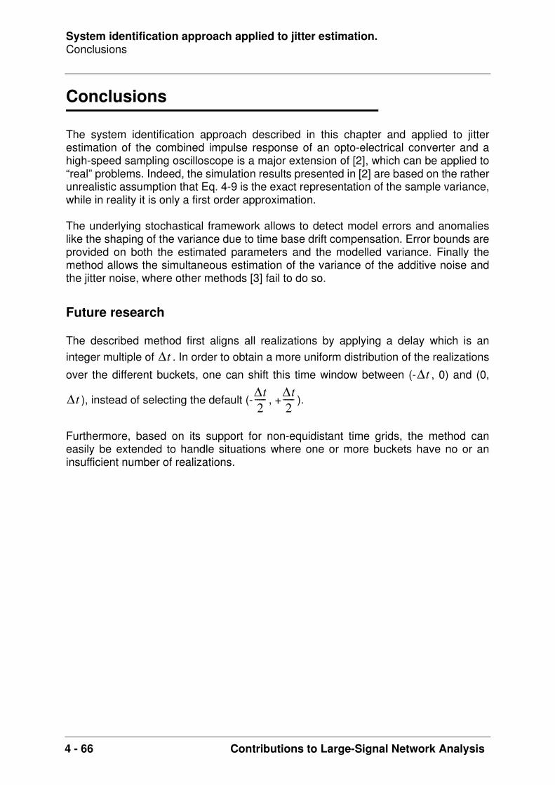
System identification approach applied to jitter estimation.Conclusions
4 - 66 Contributions to Large-Signal Network Analysis
Conclusions
The system identification approach described in this chapter and applied to jitterestimation of the combined impulse response of an opto-electrical converter and ahigh-speed sampling oscilloscope is a major extension of [2], which can be applied to“real” problems. Indeed, the simulation results presented in [2] are based on the ratherunrealistic assumption that Eq. 4-9 is the exact representation of the sample variance,while in reality it is only a first order approximation.
The underlying stochastical framework allows to detect model errors and anomalieslike the shaping of the variance due to time base drift compensation. Error bounds areprovided on both the estimated parameters and the modelled variance. Finally themethod allows the simultaneous estimation of the variance of the additive noise andthe jitter noise, where other methods [3] fail to do so.
Future research
The described method first aligns all realizations by applying a delay which is aninteger multiple of . In order to obtain a more uniform distribution of the realizations
over the different buckets, one can shift this time window between (- , 0) and (0,
), instead of selecting the default (- , + ).
Furthermore, based on its support for non-equidistant time grids, the method caneasily be extended to handle situations where one or more buckets have no or aninsufficient number of realizations.
∆t∆t
∆t ∆t2----- ∆t
2-----

System identification approach applied to jitter estimation.References
Contributions to Large-Signal Network Analysis 4 - 67
References
[1] T. Souders, D.Flach, C. Hagwood and G. Yang, “The Effects of Timing Jitter inSampling Systems,” IEEE Transactions on Instrumentation and Measurement, Vol.39, No. 1, February 1990[2] G. Vandersteen and R. Pintelon, “Maximum Likelihood Estimator for Jitter NoiseModels,” IEEE Transactions on Instrumentation and Measurement, Vol. 49, No. 6,December 2000[3] K. Coakley, C.-M. Wang, P. Hale and T. Clement, “Adaptive Characterization of Jit-ter Noise in Sampled High-Speed Signals,” IEEE Transactions on Instrumentation andMeasurement, Vol. 52, No. 5, October 2003[4] Mathematica, Wolfram Research[5] “Vector Statistical Library Notes. Intel® Math Kernel Library,” Version 6.0, July2004[6] J. Schoukens, R. Pintelon and Y. Rolain, “Maximum Likelihood Estimation ofErrors-In-Variables Models using the Sample Covariance Matrix Obtained from SmallData Sets,” published as part of “Recent Advances in Total Least Squares Techniquesand Errors-In-Variables Modeling”, Sabine Van Huffel (editor), Siam, Philadelphia,1997[7] J. Schoukens, “Inleiding in de waarschijnlijksheidsrekening en de statistiek,” VrijeUniversiteit Brussel[8] K. Coakley and P. Hale, “Alignment of Noisy Signals,” IEEE Transactions onInstrumentation and Measurement, Vol. 50, No 1., February 2001[9] Y. Rolain, J. Schoukens and G. Vandersteen, “Signal Reconstruction for Non-Equi-distant Finite Length Sample Sets: a “KIS” approach,” IEEE Transactions on Instru-mentation and Measurement, Vol. 47, No. 5, October 1998, pp. 1046 - 1052[10] G. Vandersteen, Y. Rolain and J. Schoukens, “An Identification Technique forData Acquisition Characterization in the Presence of Nonlinear Distortions and TimeBase Distortions,” IEEE Transactions on Instrumentation and Measurement, Vol. 50,No. 5, October 2001

System identification approach applied to jitter estimation.References
4 - 68 Contributions to Large-Signal Network Analysis

Contributions to Large-Signal Network Analysis 5 - 1
• “Abstract” on page 5-2
• “Modelling and estimating drift in the presence of additive and jitter noise” on page 5-3
• “Analysis of the noise sources: additive white noise” on page 5-6
• “Analysis of the noise sources: jitter noise” on page 5-10
• “The added value of the covariance matrix for the WLS” on page 5-25
• “Simulations” on page 5-27
• “Comparison to state-of-the-art methods” on page 5-30
• “Measurements” on page 5-37
• “Conclusions” on page 5-41
• “References” on page 5-42
CHAPTER 5 System identification approach applied to drift estimation.

System identification approach applied to drift estimation.Abstract
5 - 2 Contributions to Large-Signal Network Analysis
Abstract
When collecting a large number of repeated measurement records of the impulseresponse of a linear time-invariant system using a high-frequency samplingoscilloscope, it was found that the successive measurements of this impulse responseslightly shift over time, within the acquisition window. This phenomenon is referred toas time base drift.
Time base drift and its estimation in the presence of both additive and jitter noise hasalready been mentioned in this work as part of the “Enhancements to the nose-to-nose calibration technique” and during the “System identification approach applied tojitter estimation”. In this initial approach, the first measurement record is used as areference signal during the alignment of successive measurements. This givesestimates, which are comparable to the ones based on the method proposed in [1].Here, an enhanced version of the initial approach is proposed. In this method, thealigned average is used as a reference signal instead of the first measurement.
A system identification approach is applied to estimate the time base drift introducedby a high-frequency sampling oscilloscope. First, a new least squares estimator isproposed to estimate the delay of a set of repeated measurements in the presence ofadditive and jitter noise. Next, the effect of both additive and jitter noise is studied inthe frequency domain using simulations.
Special attention is devoted to the covariance matrix of the experiments. The use ofthis matrix allows to come up with a good estimate of the uncertainty on the estimateddelays. Using the covariance matrix, a weighted least squares estimator isimplemented to minimize the uncertainty on the estimated delays. Comparativeresults are shown based on simulations proposed by [1].
Finally, the enhanced method is applied to estimate the drift using the samemeasurements as those that were used during the jitter estimation. The impulseresponse of an opto-electrical converter is measured using an Agilent 83480Asampling oscilloscope in combination with a 83484A 50 GHz electrical plug-in.

System identification approach applied to drift estimation.Modelling and estimating drift in the presence of additive and jitter noise
Contributions to Large-Signal Network Analysis 5 - 3
Modelling and estimating drift in the presence of additive and jitter noise
High-frequency sampling oscilloscopes often use an equivalent-time samplingprinciple to diminish the needed conversion rate. They suffer from both additivemeasurement noise and timing jitter noise at the sampling time instant
. Furthermore, it is observed that these oscilloscopes also suffer from time base
drift. Time base drift is due to imperfections on the position of the trigger point relativeto the signal and results in a movement of the signal in the acquisition window. As aresult, successive measurements correspond to delayed versions of the “exact”signal. The delay models this effect and varies with respect to the realization index
. The resulting signal model is
Eq. 5-1
Herein, represents the -th measurement of the exact signal when
both additive noise and jitter are added as a part of the measurement. Both
and are assumed to be zero mean, normally distributed, independent and
stationary with respect to , and as a result they are also independent with respect to
realization index . Furthermore, it is assumed that . represents the
sampling period.
Let correspond to the discrete Fourier transform of . As part of the
enhancements to the nose-to-nose calibration technique and the system identificationapproach applied to jitter estimation, the time base drift of each acquisition wasestimated using the first acquisition as a reference signal. In the approach proposedhere, the (unknown) exact signal is used as the reference signal. The LS cost functionthen becomes
Eq. 5-2
Eq. 5-2 must be minimized with respect to both the unknown delays and the
Fourier coefficients of the unknown exact signal . Since the spectra
appear linearly in the equation error, it is possible to eliminate them from the cost.Therefore, the symbolic derivative of Eq. 5-2 with respect to is set to zero1.
ny ti( ) nt ti( )
ti
τk
k
yk ti( ) y0 ti nt ti( ) τk+ +( ) ny ti( )+=
yk ti( ) k y0 ti( )
ny ti( )
nt ti( )
tk ti i t∆= t∆
Yk ωm( ) yk ti( )
VLS Yk ωm( ) e jωmτk– Y0 ωm( )⋅– 2
k m,=
τk
Y0 ωm( ) Y0 ωm( )
Y0 ωm( )

System identification approach applied to drift estimation.Modelling and estimating drift in the presence of additive and jitter noise
5 - 4 Contributions to Large-Signal Network Analysis
Eq. 5-3
Eq. 5-4
Here corresponds to the complex conjugate of . can now be calculated
as follows:
. Eq. 5-5
represents the number of repeated realizations of delayed versions of .
Substituting Eq. 5-5 in Eq. 5-2 and using the fact that , results in a cost
function which is only a function of the unknown delays :
Eq. 5-6
It is possible to introduce an arbitrary delay as follows
, , Eq. 5-7
without influencing . If is considered to be the new
reference, it is clear that there is a degeneracy: (only) one delay can be freely chosen.One possibility is to select one delay to be zero. For example, here it is assumed that
.
1. Since the function VLS is not an analytical form in Y0 due to the presence of the complex conjugate, this deserves some additional explanation (see page 5-5).
Y0 ωm( )∂∂VLS 0=
Yk ωm( ) e jωmτk– Y0 ωm( )⋅–[ ]∗
k e jωmτk––( )⋅ 0=⇔
Y∗ Y Y0 ωm( )
Y0ˆ ωm( ) 1
K---- Yk ωm( ) ejωmτk⋅
k 1=
K
=
K Y0 ωm( )
e jθ– 1=τk
VLS τ1 .. τK, ,( ) Yk ωm( ) ejωmτk⋅ 1K---- Yl ωm( ) ejωmτl⋅
l 1=
K
–
2
k m,=
τ
Yk ω( ) e jωτk– Y0 ω( )⋅ e jω τk τ+( )– Y0 ω( ) ejωτ⋅[ ]⋅= = k 1.. K=
VLS Y0˜ ω( ) Y0 ω( ) ejωτ⋅=
τ1 0=

System identification approach applied to drift estimation.Modelling and estimating drift in the presence of additive and jitter noise
Contributions to Large-Signal Network Analysis 5 - 5
The derivatives of Eq. 5-6 with respect to up to yield the gradient while the
second derivatives yield the Hessian of the cost. The Newton-Raphson iterationscheme is then used to find the estimates which minimize Eq. 5-6, given
that .
Starting values are readily available from the initial implementation1 (also imposing) which uses the first realization as reference signal, instead of the
average signal, as is obtained after the alignment of the records.
Although these starting values reduce the number of iterations that are needed toconverge to the solution, it was found that zero starting values also do the job. Evenstarting values where the sign of the delay is incorrect still lead to convergence to thesame solution. This shows the robustness of the method to poor starting values.
Symbolic derivation
To justify the use of symbolic derivatives [2] with respect to Eq. 5-2, consider
as an alternative for , where represents the complex
conjugate of .
Eq. 5-8
Eq. 5-9
Based on Eq. 5-8 and Eq. 5-9, and given , it is clear that
Eq. 5-10
1. As described as part of the “Enhancements to the nose-to-nose calibration technique” and during the “System identification approach applied to jitter estimation”.
τ2 τK
τ2 .. τK, ,
τ1 0=
τ1 0= Y1 ω( )
f x x∗,( ) |R∈ f xR xI,( ) x∗
x xR jxI+=
xR∂∂f
x∂∂f
xR∂∂x⋅
x∗∂∂f x∗∂
xR∂---------⋅+
x∂∂f
x∗∂∂f+= =
xI∂∂f
x∂∂f
xI∂∂x⋅
x∗∂∂f x∗∂
xI∂--------⋅+ j
x∂∂f
x∗∂∂f–
= =
x∗∂∂f
x∂∂f
∗=
xR∂∂f
xI∂∂f 0= = Re
x∂∂f⇔ Im
x∂∂f 0= =
x∂∂f 0=⇔

System identification approach applied to drift estimation.Analysis of the noise sources: additive white noise
5 - 6 Contributions to Large-Signal Network Analysis
Analysis of the noise sources:additive white noise
Is the noise circular complex distributed?
For personal educational purposes, first it is verified that the assumption of circularcomplex noise in the frequency domain holds in the case of additive noise, which isstationary with respect to time. To this end, realistic simulations will be used. Thecovariance matrix of the noise in the frequency domain is obtained as a by-product,and is based on covariance information in the time domain.
In order to keep the simulation as realistic as possible, the analytical expression of theimpulse response that has been used during the system identification approachapplied to jitter estimation is reused here.
500 realizations of this impulse response are generated in the presence of additivenoise, which is chosen to be zero mean, is normally distributed and is stationary withrespect to time. The standard deviation is chosen to be 3 mV. The delay is set to zero.
A scaling factor of is used during the calculation of the discrete Fourier transform
( represents the number of time points within each realization of the simulation).
Starting from a variance = 9x10⁻⁶ V2 at each time instant, it is found that 9x10⁻⁶
falls inside the 95% confidence interval of the resulting sample variance at eachfrequency.
As can be expected, the additive noise shows up as circular complex white noise in
the frequency domain, with and , i.e. the variance of the
real part of the spectrum equals that of the imaginary part, while there is nostochastically significant correlation between the real and the imaginary part.Furthermore, the variance does not vary and is uncorrelated as a function of thefrequency.
The calculation of the covariance in the frequency domain is based on the linearrelationship between the Fourier coefficients and the time samples. Therefore
, Eq. 5-11
where represents the hermitian transpose of , with .
NN
σ2
σR2 σI
2 σ2
2------= = σRI
20=
Cov Y ω( )[ ] J Cov y t( )[ ] JH⋅ ⋅=
J H J Jmi
Y ωm( )∂y ti( )∂
-------------------=

System identification approach applied to drift estimation.Analysis of the noise sources: additive white noise
Contributions to Large-Signal Network Analysis 5 - 7
In the case where and , , .
Using Eq. 5-11 in the special case , where represents a
identity matrix, one finds the known result: .
Weighted version of VLS
In the case of only additive white noise, . It is then simple toobtain the expected value of the cost function, which is easy to interpret if Eq. 5-2 is
divided by . A scale factor of is consistently used during the calculation of theFFT. This allows simple validation of the model by comparison of the value of the costfunction taken in the estimates to the expected cost.
Given the number of realizations of the measurement and the number of
frequency components used to estimate the delays, the expected value of the costequals the number of measurement data minus the number of parameters, i.e.
.
As a quick sanity check, three sets of 500 realizations (all = 0) of the impulse
response are generated, one with = 0.6 mV and two with = 3 mV. The samesignal is used as during the preceding tests. If one takes frequency components up to100 GHz into account, 500 frequency components are used in the case of a frequencyresolution of 200 MHz. The expected value of the cost is 249500 while the 95%
confidence interval for the - distributed cost equals = 1413. Allthree realized cost functions (248899, 248900 and 249757) fall inside the 95%confidence interval of the expected cost.
Verification of the uncertainty on the estimated delays
Again, only additive noise with is considered to be present.One obtains an estimate of the parameter covariance matrix [3]:
Eq. 5-12
ti i ∆t⋅= ωm2πmN ∆t⋅--------------= Jmi
1N
-------- e2π j mi
N------–
= j 1–=
Cov y t( )[ ] σ2 I⋅= I N N×
Cov Y ω( )[ ] σ2 J J H⋅ ⋅ σ2 I⋅= =
Cov Y ω( )[ ] σ2 I⋅=
σ2 N
K MK
E VLS K M 1–( )⋅=
τk
σ σ
χ2 2 2K M 1–( )⋅
Cov Y ω( )[ ] σ2 I⋅=
Cov τ[ ] 2re JHJ( )[ ]
1–2re J
HCov Y ω( )[ ] J( ) 2re J
HJ( )[ ]
1–⋅ ⋅≅

System identification approach applied to drift estimation.Analysis of the noise sources: additive white noise
5 - 8 Contributions to Large-Signal Network Analysis
Eq. 5-13
Here corresponds to the Jacobian of the complex error vector ;
is the vector equivalent of Eq. 5-6.
If one considers 500 realizations of the impulse response and 500 frequencycomponents per experiment, the Jacobian is a 250,000 by 499 complex matrix.Therefore, initially the calculation of the Jacobian is avoided. In the absence of modelerrors and, when evaluated in the solution, Eq. 5-13 can be approximated by
, Eq. 5-14
where represents the Hessian, i.e. the second derivative of the cost function (Eq.
5-2) with respect to the estimated parameters . The inverse Hessian is
readily available as a part of the Newton-Raphson algorithm.
The same sanity check as was mentioned above shows that for the two realizations ofthe impulse response with = 3 mV, the uncertainty on the estimated delays basedon the inverse Hessian is found to be 70.9 fs. It lies once within and once just outside
the 95% confidence interval of the observed uncertainties (based on a -
distribution, resp. 61.3 fs .. 69.6 fs and 63.5 fs .. 72.1 fs).
A more detailed inspection of the parameter covariance matrix shows a correlationcoefficient between any two delays which approximates 0.5 for all estimated delays.Although initially this might come as a surprise, a correlation coefficient of 0.5 caneasily be explained. Indeed, because of the constraint that was set to 0, the
remaining estimates in fact correspond to estimates of
where , are assumed to be identically distributed and uncorrelated.
As such, for
Eq. 5-15
Cov τ[ ] 2re J HJ( )[ ]1–
σ2⋅≅
J J e τ( )∂τ∂
-------------= e τ( )
VLS τ( ) e H τ( ) e τ( )⋅=
Cov τ[ ] H 1– σ2⋅≅
Hτ2 .. τK, ,
σ
χ5002
τ1
τ2 .. τK, , τ2 τ1 .. τK τ1–, ,–
τk k 1 .. K, ,=
k l≠
στkτl
2 E τk E τk –( ) τl E τl –( )[ ]=
E τk τ1– E τk τ1– –( ) τl τ1– E τl τ1– –( )[ ]=
E τ1 E τ1 –( )2
[ ] α==

System identification approach applied to drift estimation.Analysis of the noise sources: additive white noise
Contributions to Large-Signal Network Analysis 5 - 9
while for
Eq. 5-16
The correlation coefficient therefore equals to .
k l=
στkτk
2E τk E τk –( )2[ ]=
E τk τ1– E τk τ1– –( )2
[ ]=
E τ1 E τ1 –( )2
[ ] E τk E τk –( )2
[ ]+ 2α==
ρστkτl
2
στkτk
2------------ α
2α------- 1
2---= = =

System identification approach applied to drift estimation.Analysis of the noise sources: jitter noise
5 - 10 Contributions to Large-Signal Network Analysis
Analysis of the noise sources:jitter noise
The next logical step is to study the influence of jitter noise on the measurements inthe frequency domain. The additive noise is set to zero.
The jitter noise is assumed to be zero mean, normally distributed, independent
and stationary with respect to . Its standard deviation is assumed to be known and isset equal to 1 ps.
First, the study is performed based on simulations using the sample variance of thereal and the imaginary part of the spectral data corresponding to the realizations of thesame known signal1 as before that is disturbed by jitter noise only.
Next, the covariance matrix in the frequency domain is calculated based on thecovariance matrix in the time domain. For the considered jitter noise, the latterreduces to a diagonal matrix. The values on the diagonal correspond to the varianceand their value depends on the derivatives of the underlying signal with respect to .
In order to minimize the variation of the phase spectrum of the considered impulseresponse as a function of the frequency, the analytical expression of the impulseresponse is adapted such that its peak value is located at . This way, thedeterministic portion of the variation of the real and the imaginary part of the spectrum,when taken as a function of the frequency, is minimized.
Simulation results
Figure 5-1 shows the sample mean of 5000 realizations of the considered impulseresponse. Figure 5-2 zooms in on the left edge of the time window and clearly showsthat the peak value of the impulse response is located at .
Figure 5-3 and figure 5-4 show the corresponding sample variance of the signalsshown in figure 5-1 and figure 5-2.
Although it has no physical meaning, it is useful to take a look at the discrete Fouriertransform of the sample variance. Later, it will become apparent that there is arelationship between this Fourier transform and the sample variance of the real andthe imaginary part of the spectrum of the 5000 realizations. Figure 5-5 and figure 5-6respectively show the real and the imaginary part of the Fourier transform of the
1. Again, the same analytical expression of the impulse response is used as during the system identifi-cation approach applied to jitter estimation.
nt ti( )
t
t
t 0=
t 0=

System identification approach applied to drift estimation.Analysis of the noise sources: jitter noise
Contributions to Large-Signal Network Analysis 5 - 11
sample variance (figure 5-3).
Figure 5-7 and figure 5-8 show the sample variance of the real and the imaginary partof the spectrum for the 5000 realizations of the impulse response.
Figure 5-1. Sample average of the impulse response disturbed by jitter noise.
Figure 5-2. Sample average of the impulse response disturbed by jitter noise(zoomed in around t = 0).
1 2 3 4 5time ns
0.02
0.02
0.04
0.06
0.08
mean V
0.02 0.04 0.06 0.08 0.1time ns
0.02
0.02
0.04
0.06
0.08
mean V

System identification approach applied to drift estimation.Analysis of the noise sources: jitter noise
5 - 12 Contributions to Large-Signal Network Analysis
Visual comparison of figure 5-5 and figure 5-7 suggests that there is a relationshipbetween the Fourier transform of the sample variance of the signal and the samplevariance of the Fourier transform of the signal, especially when taking the folding ofthe frequency axis by a factor of 2 into account. This is explained in more detail onpage 5-20.
Figure 5-3. Sample variance of the impulse response disturbed by jitter noise.
Figure 5-4. Sample variance of the impulse response disturbed by jitter noise(zoomed in around t = 0).
1 2 3 4 5time ns
0.025
0.05
0.075
0.1
0.125
0.15
0.175
var x103 V2
0.02 0.04 0.06 0.08 0.1time ns
0.025
0.05
0.075
0.1
0.125
0.15
0.175
var x103 V2

System identification approach applied to drift estimation.Analysis of the noise sources: jitter noise
Contributions to Large-Signal Network Analysis 5 - 13
Calculating the sample variance of realizations of a complex number
as , it is clear that equals the
sum of the sample variance of the real and the imaginary part of that number.
Figure 5-5. Real part of the Fourier transform of the sample variance (figure 5-3).
Figure 5-6. Imaginary part of the Fourier transform of the sample variance (figure 5-3).
200 400 600 800freq GHz
0.2
0.1
0.1
0.2
0.3
0.4
re var x106 V2
200 400 600 800freq GHz
0.1
0.05
0.05
0.1
im var x106 V2
σx K,2 K x k( ) x
σx K,2 1
K 1–------------- x k( ) 1
K---- x l( )
l 1=K
–2
k 1=K
= σx K,2

System identification approach applied to drift estimation.Analysis of the noise sources: jitter noise
5 - 14 Contributions to Large-Signal Network Analysis
Figure 5-9 shows this sample variance for the spectrum of the 5000 realizations of theimpulse response. Taking into account the width of the 95% confidence interval, it isacceptable to consider that this value is a constant as a function of the frequency.
Using the 95% confidence interval of a distribution, this was verified for the
Figure 5-7. Sample variance of the real part of the Fourier transform of the 5000 realizations of the impulse response.
Figure 5-8. Sample variance of the imaginary part of the Fourier transform of the 5000 realizations of the impulse response.
200 400 600 800freq GHz
0.1
0.2
0.3
0.4
0.5var re x106 V2
200 400 600 800freq GHz
0.1
0.2
0.3
0.4
0.5var im x106 V2
χ2

System identification approach applied to drift estimation.Analysis of the noise sources: jitter noise
Contributions to Large-Signal Network Analysis 5 - 15
frequency band where there is no apparent correlation between the noise on the realand the imaginary part. Correct calculation of the 95% confidence interval in case acorrelation is present, requires the use of the Wishart distribution [4] and is not dealtwith at this moment.
Another important verification is to check whether the correlation between the real andthe imaginary part of the spectrum is not significant and the result is shown in figure 5-10. The correlation coefficient of two stochastical quantities and is defined as
. Eq. 5-17
Figure 5-11 zooms in to the lower frequency band and shows the correlation betweenthe noise on the real and the imaginary part of the spectrum up to about 65 GHz.Correct calculation of the 95% confidence interval requires additional work and is notprovided1.
Next it makes sense to look at the 5000 realizations of the real and the imaginaryvalue of the spectrum at some frequencies of interest:
• at 4 GHz: the correlation has its largest negative value
Figure 5-9. Sample variance of the Fourier transform of the 5000 realizations of the impulse response.
1. However, visual comparison of figure 5-11 and figure 5-18 shows good correspondence, the latter being calculated starting from the variance in the time domain.
200 400 600 800freq GHz
0.1
0.2
0.3
0.4
0.5var x106 V2
ρ x y
ρσxy
2
σx σy⋅----------------=

System identification approach applied to drift estimation.Analysis of the noise sources: jitter noise
5 - 16 Contributions to Large-Signal Network Analysis
• at 38 GHz: the correlation changes from a negative to a positive value• at 50 GHz: the correlation has its largest positive value• at 70 GHz: no correlation is present between the real and the imaginary part
Figure 5-10. Correlation coefficient of the real and the imaginary part of the Fourier transform of the 5000 realizations of the impulse response.
Figure 5-11. Correlation coefficient of the real and the imaginary part of the Fourier transform of the 5000 realizations of the impulse response (DC up to 80 GHz).
200 400 600 800freq GHz
0.4
0.2
0.2
0.4
ρ re,im
10 20 30 40 50 60 70 80freq GHz
0.4
0.2
0.2
0.4
ρ re,im

System identification approach applied to drift estimation.Analysis of the noise sources: jitter noise
Contributions to Large-Signal Network Analysis 5 - 17
Figure 5-12 up to figure 5-15 show the results using a 1:1 aspect ratio for all plots.
Clearly the assumption that the spectral noise is circular complex is not valid,especially at lower frequencies. The bandwidth where the correlation is significantdepends on the measured signal itself.
Figure 5-12. 5000 realizations of the real and the imaginary value of the spectrum at 4 GHz (maximum negative correlation ).
Figure 5-13. 5000 realizations of the real and the imaginary valueof the spectrum at 38 GHz (zero correlation, but clearly not circular).
10 11 12 13 14re mV
10.750.5
0.25
0.250.5
0.751
im mV
0.4–≅
9.5 10 10.5 11re mV
1
2
3
im mV

System identification approach applied to drift estimation.Analysis of the noise sources: jitter noise
5 - 18 Contributions to Large-Signal Network Analysis
In the presence of jitter noise, the covariance matrix in the frequency domain musttake into account the contributions of the real and the imaginary part of the spectrumseparately.
Furthermore, one can take a look at the correlation between spectral contributionsoriginating from different frequencies (real, real), (real, imag), (imag, real) and (imag,imag). Correlation is observed up to about 130 GHz.
Calculation of the covariance matrix of the spectral noise in the frequency domain
It is shown that it is possible to calculate the covariance matrix in the frequencydomain, if one has an estimate of the variance in the time domain. The time domainvariance has been obtained in the chapter on jitter estimation. There, it isdemonstrated that it is indeed possible to estimate the standard deviation of both theadditive and the jitter noise, hence also the variance as a function of time. Thisinformation can be used to come up with an estimate of the covariance matrix in thefrequency domain. This allows to obtain an optimal scaling of each frequencycontribution of the cost function in the sense that it becomes possible to know theexpected value of the cost in advance and to minimize and estimate the uncertaintyon the estimated delays.
Figure 5-14. 5000 realizations of the real and the imaginary valueof the spectrum at 50 GHz (maximum positive correlation ).
5.5 6 6.5 7 7.5re mV
4.5
3.5
3
2.5
2
1.5
1
im mV
0.2≅

System identification approach applied to drift estimation.Analysis of the noise sources: jitter noise
Contributions to Large-Signal Network Analysis 5 - 19
Because the above simulations show that the noise is not circular complex, thefrequency covariance matrix must take the real and the imaginary part of the spectruminto account separately. The covariance matrix in the frequency domain can then becalculated similar to Eq. 5-11, provided that the real and the imaginary part areseparated.
Eq. 5-18
In Eq. 5-18, represents the transpose of the Jacobian matrix ,whichis the matrix notation of the discrete Fourier transform where the odd rows correspondto the real part and the even rows to the imaginary part of the Fourier coefficient.
represents the number of frequency components of interest and is the number oftime points of one realization of the impulse response. The covariance matrix in the
time domain reduces to a diagonal matrix in case the jitter isnot correlated as a function of time. The values on this diagonal correspond to thevariance as function of time. Based on the analytical expression of the impulseresponse and the standard deviation of the jitter, it is possible to calculate the requiredderivatives of the signal with respect to time and hence to obtain the variance as afunction of time.
Figure 5-15. 5000 realizations of the real and the imaginary value of the spectrum at 70 GHz (no correlation, circular complex noise).
1.5 1 0.5 0.5 1 1.5re mV
1.5
1
0.5
0.5
1
1.5
im mV
Cov Y ω( )[ ] J Cov y t( )[ ] J T⋅ ⋅=
J T J |R2M N×∈
MN
Cov y t( )[ ] |RN N×∈

System identification approach applied to drift estimation.Analysis of the noise sources: jitter noise
5 - 20 Contributions to Large-Signal Network Analysis
Eq. 5-19
In the chapter on jitter estimation, for the considered impulse response, Eq. 5-19 wasfound to provide a very good approximation for the variance in the case of Gaussianjitter that has a standard deviation less than or equal to 1 ps.
The rows of the Jacobian matrix contain the coefficients of the discrete
Fourier transform that yield the real and the imaginary part of the th frequency
component. In the case is a diagonal matrix with on the diagonal,
the sum of each row of corresponds to the real, resp. the imaginarypart of the Fourier transform of the variance as function of time.
, Eq. 5-20
For the diagonal terms of , the matrix product yields
for the even rows,
for the odd rows.
This is not equal to the real and the imaginary part of . The
latter corresponds to a scaled version of Eq. 5-20, except for the fact that the complex
exponential is now replaced by with . It looks as if
is divided by a factor of 2 and therefore the frequency axis appears to be folded by
σy3
2ti( )
td
dy0
2
t ti=
σnt
2⋅=
12---
t2
2
d
d y0
2
⋅td
dy0
t3
3
d
d y0⋅+
t ti=
σnt
4⋅ 512------
t3
3
d
d y0
2
t ti=
σnt
6⋅ ⋅+ +
2k 2k 1+, Jk
Cov y t( )[ ] σy3
2ti( )
J Cov y t( )[ ]⋅
ΣY3
2m( ) 1
N-------- σy3
2i( ) e
j2πmi N⁄–⋅
i 0=
N 1–
= m 0 .. N 1–=
Cov Y ω( )[ ] J Cov y t( )[ ] JT⋅ ⋅
1N---- σy3
2i( ) 2πki N⁄( )cos
2⋅
i 0=
N 1–
1N---- σy3
2i( ) 2πki N⁄( )sin
2⋅
i 0=
N 1–
1N---- σy3
2 i( ) e j4πki N⁄–⋅
i 0=
N 1–
e j2πkn N⁄– e j2πkn N '⁄– N ' N2----=
N

System identification approach applied to drift estimation.Analysis of the noise sources: jitter noise
Contributions to Large-Signal Network Analysis 5 - 21
a factor of 2. This explains both the apparent similarity and the difference (seefigure 5-5 up to figure 5-8) between the sample variance of the spectral data and thespectral data corresponding to the sample variance.
Figure 5-16. Variance as a function of the frequency using Eq. 5-18 and Eq. 5-19 (even rows).
Figure 5-17. Variance as a function of the frequency using Eq. 5-18 and Eq. 5-19 (odd rows).
100 200 300 400freq GHz
0.1
0.2
0.3
0.4
0.5var re x106 V2
100 200 300 400freq GHz
0.1
0.2
0.3
0.4
0.5var im x106 V2

System identification approach applied to drift estimation.Analysis of the noise sources: jitter noise
5 - 22 Contributions to Large-Signal Network Analysis
Figure 5-16 and figure 5-17 show the variance as function of frequency, based on Eq.
5-18 and Eq. 5-19 for the even and odd rows of the diagonal of .
The sum of both turns out to be 0.422 10-6 V2, is constant as a function of thefrequency and corresponds to the mean value of the sample variance shown infigure 5-9. When comparing figure 5-16 and figure 5-17 to figure 5-7 and figure 5-8, itshould be noted that, due to memory limitations, the number of time points wasreduced from 4096 to 2048. This explains the decrease of the sampling frequencywith respect to figure 5-7 and figure 5-8.
Figure 5-18 is the equivalent of figure 5-11, but is now calculated based on thecovariance matrix, obtained using Eq. 5-18.
Finally, the artwork resulting from the contour plots of each portion ((re,re), (re,im),(im,re) and (im,im)) of the frequency covariance matrix is shown in figure 5-19 up tofigure 5-22. White is mapped onto the largest value and black to the smallest value.
It can be concluded that an estimate of the variance in the time domain (Eq. 5-19)allows to construct the full covariance matrix in the frequency domain.
Figure 5-18. Correlation coefficient of the real and the imaginary part using Eq. 5-18 andEq. 5-19.
Covariance min. value (V2) max. value (V2)(re,re) -0.183 µ 0.422 µ(im,im) -0.303 µ 0.303 µ(re,im) and (im,re) -0.117 µ 0.117 µ
Table 5-1. Min. and max. values of the different portions of the frequency covariance matrix.
J Cov y t( )[ ] J T⋅ ⋅
10 20 30 40 50 60 70 80freq GHz
0.4
0.2
0.2
0.4
ρ re,im
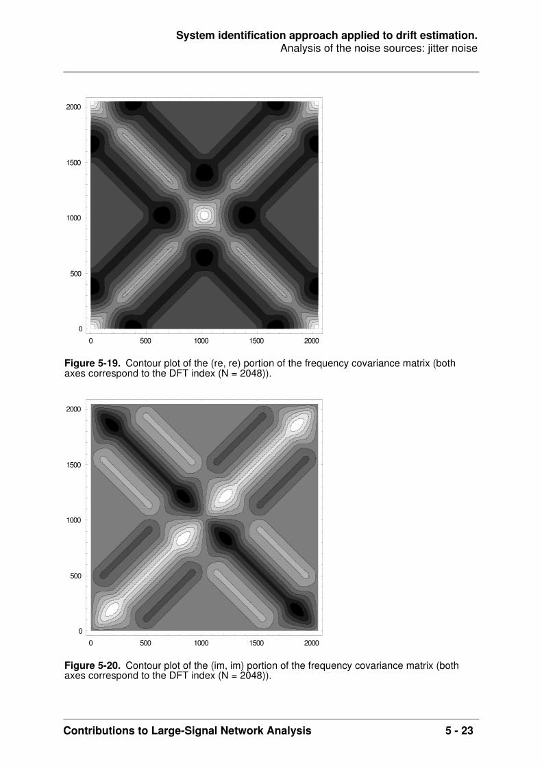
System identification approach applied to drift estimation.Analysis of the noise sources: jitter noise
Contributions to Large-Signal Network Analysis 5 - 23
Figure 5-19. Contour plot of the (re, re) portion of the frequency covariance matrix (both axes correspond to the DFT index (N = 2048)).
Figure 5-20. Contour plot of the (im, im) portion of the frequency covariance matrix (both axes correspond to the DFT index (N = 2048)).
0 500 1000 1500 2000
0
500
1000
1500
2000
0 500 1000 1500 2000
0
500
1000
1500
2000
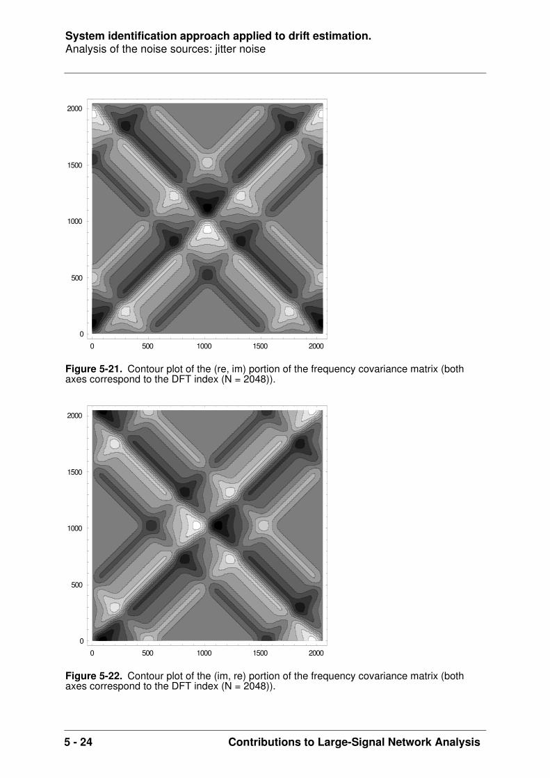
System identification approach applied to drift estimation.Analysis of the noise sources: jitter noise
5 - 24 Contributions to Large-Signal Network Analysis
Figure 5-21. Contour plot of the (re, im) portion of the frequency covariance matrix (both axes correspond to the DFT index (N = 2048)).
Figure 5-22. Contour plot of the (im, re) portion of the frequency covariance matrix (both axes correspond to the DFT index (N = 2048)).
0 500 1000 1500 2000
0
500
1000
1500
2000
0 500 1000 1500 2000
0
500
1000
1500
2000
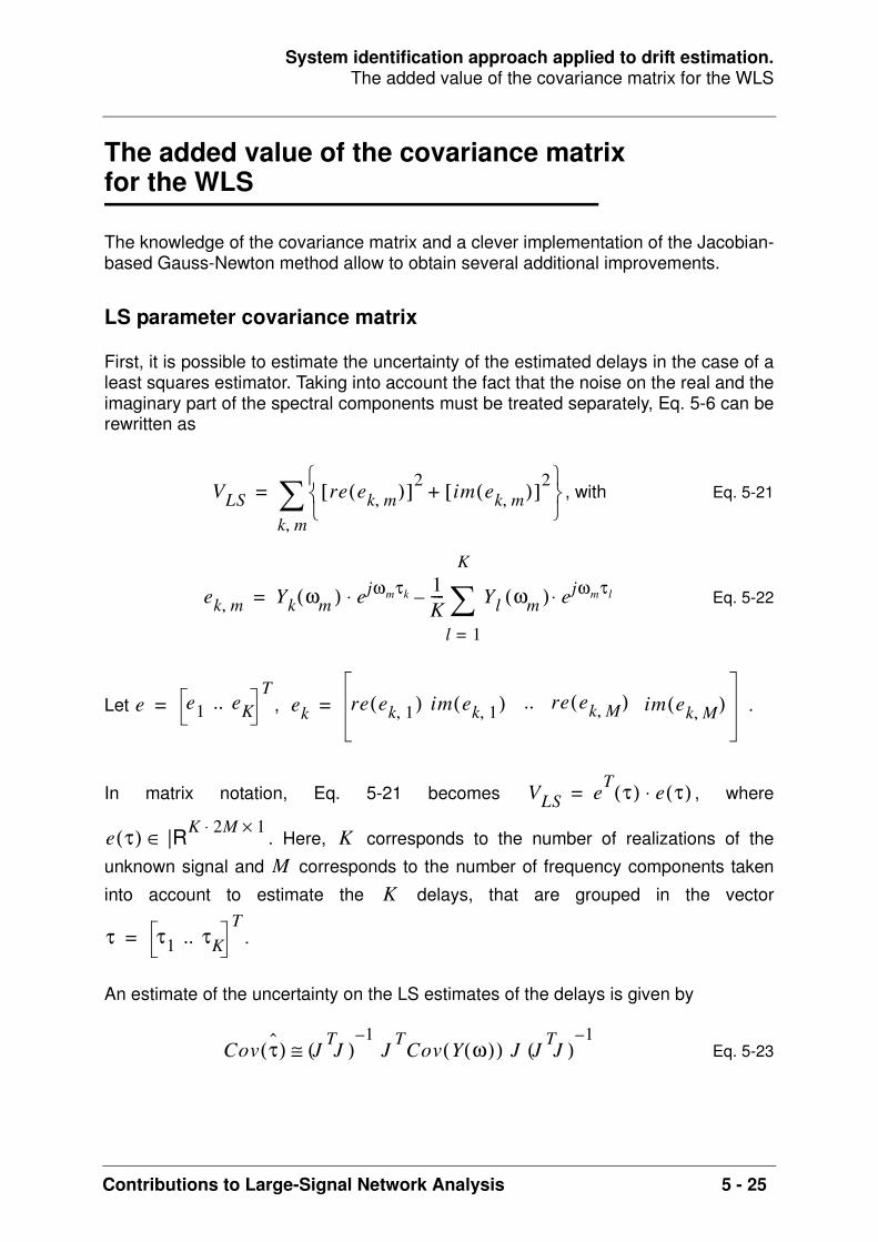
System identification approach applied to drift estimation.The added value of the covariance matrix for the WLS
Contributions to Large-Signal Network Analysis 5 - 25
The added value of the covariance matrixfor the WLS
The knowledge of the covariance matrix and a clever implementation of the Jacobian-based Gauss-Newton method allow to obtain several additional improvements.
LS parameter covariance matrix
First, it is possible to estimate the uncertainty of the estimated delays in the case of aleast squares estimator. Taking into account the fact that the noise on the real and theimaginary part of the spectral components must be treated separately, Eq. 5-6 can berewritten as
, with Eq. 5-21
Eq. 5-22
Let , .
In matrix notation, Eq. 5-21 becomes , where
. Here, corresponds to the number of realizations of the
unknown signal and corresponds to the number of frequency components taken
into account to estimate the delays, that are grouped in the vector
.
An estimate of the uncertainty on the LS estimates of the delays is given by
Eq. 5-23
VLS re ek m,( )[ ]2 im ek m,( )[ ]2+
k m,=
ek m, Yk ωm( ) ejωmτk⋅ 1K---- Yl ωm( ) ejωmτl⋅
l 1=
K
–=
e e1 .. eKT
= ek re ek 1,( ) im ek 1,( ) .. re ek M,( ) im ek M,( )=
VLS eT τ( ) e τ( )⋅=
e τ( ) |RK 2M⋅ 1×∈ KM
K
τ τ1 .. τKT
=
Cov τ( ) JTJ( )
1– J
TCov Y ω( )( ) J J
TJ( )
1–≅

System identification approach applied to drift estimation.The added value of the covariance matrix for the WLS
5 - 26 Contributions to Large-Signal Network Analysis
where represents the Jacobian and equals . Based on the degeneracy
mentioned earlier (Eq. 5-7), is again fixed equal to zero and the Jacobian matrix
looses one column: , while .
Typical values for both and in an experimental environment are 500. Thisresults in a large Jacobian matrix of size 500,000 x 499 and a covariance matrix of1000 x 1000. Fortunately, there is some structure in the Jacobian matrix derived fromEq. 5-22, such that the problem can be solved in blocks of size .
WLS estimator
Secondly, it is possible to construct a weighted least squares estimator whichminimizes the uncertainty on the estimated delays and, at the same time, has a knownexpected value of the cost function, such that the obtained cost function can becompared to its expected value. This criterion can then be used to detect modelerrors.
Eq. 5-24
The advantages of this method will become apparent when it will be applied to bothsimulations and measurements.
J e τ( )∂τ∂
-------------
τ1
J |RK 2M⋅ K 1–( )×∈ Cov Y ω( )( ) |R2M 2M×∈
K M
2M K 1–( )×
VWLS eT τ( ) Cov Y ω( )( )[ ] 1–
e τ( )⋅ ⋅=

System identification approach applied to drift estimation.Simulations
Contributions to Large-Signal Network Analysis 5 - 27
Simulations
A first set of simulations is based on the same analytical expression of the impulseresponse as the one that is used during the simulations of the jitter estimation. Thedrift is estimated in the presence of both additive and jitter noise. The jitter noise andthe additive noise are set to have realistic values: both are Gaussian, zero mean witha standard deviation of respectively 1 ps and 0.6 mV. The exact signal is assumed tobe known. Therefore, using Eq. 5-18 and Eq. 5-19, one can calculate .
Each simulation consists of 500 realizations of the signal. Hence, . Eachrealization contains 4096 time samples of the impulse response, which spans anacquisition window of 5 ns. If the spectral components are taken into account up to100 GHz, then .
Estimators
Different estimators are compared:
• based on Eq. 5-2, using the first realization as a reference instead of the aligned sample average. Inspired by the terminology used in [1], this estimator will be referred to as the “naive” LS estimator.• the “enhanced” LS estimator, corresponding to Eq. 5-6, uses the aligned sample average as reference.• the “enhanced” WLS estimator, based on Eq. 5-24, also uses the aligned sample average as reference and adds weighting based on the inverse full covariance matrix. This takes the uncertainty on the real and the imaginary part into account separately.
Zero drift
During the first simulation, the drift is set to be exactly zero. Due to the jitter noise andthe additive noise, the estimated drift is not exactly zero, however, but rather becomesa stochastical variable. Because of the degeneracy, demonstrated by Eq. 5-7, only itsstandard deviation is shown in Table 5-2.
Estimator Uncertainty of estimated (ps) 95% confidence interval (ps) of
naive LS 0.260 0.245 .. 0.277
enhanced LS 0.253 0.238 .. 0.270
enhanced WLS 0.132 0.124 .. 0.141
Table 5-2. Uncertainty of the estimated drift (case where the exact drift is zero).
Cov Y ω( )( )
K 500=
M 500=
στ τ στ

System identification approach applied to drift estimation.Simulations
5 - 28 Contributions to Large-Signal Network Analysis
Table 5-2 clearly shows that the naive and the enhanced LS estimator obtain thesame performance. Their uncertainties lie inside their respective confidence intervals.The enhanced WLS estimator reduces the uncertainty on the estimated delay byabout a factor 2.
If, in the presence of jitter, the noise in the frequency domain is assumed to be circularcomplex noise, the uncertainty on the estimated delay for the enhanced LS estimatorbased on the parameter covariance matrix (Eq. 5-14) equals 0.021 ps. Hence, itunderestimates the obtained uncertainty by a factor of more than 10. Using the fullcovariance matrix (Eq. 5-23), the estimated uncertainty on the delay turns out to be0.242 ps and this value falls within the 95% confidence interval of the obtaineduncertainty.
In the case of the enhanced WLS estimator, the expected value of the cost is499500 ± 1999. The realized cost turns out to be 497250 and falls within the 95%confidence interval of the expected value of the cost. It can thus be concluded thatthere are no detectable model errors1.
Linear drift
During the second simulation, the drift is known to be a linear function of therealization index. Applying a delay of 0.01 ps per realization, the drift of the firstrealization is zero, while that of the 500th realization is known to be 4.99 ps.
1. relative to the variance of the measurements.
Figure 5-23. Using the enhanced LS estimator (case of linear drift).
100 200 300 400 500
realizationindex
1
2
3
4
5
estimatedTBDt ps

System identification approach applied to drift estimation.Simulations
Contributions to Large-Signal Network Analysis 5 - 29
Figure 5-23 shows the results for the enhanced LS estimator, which turns out to bevisibly indistinguishable from that of the naive LS estimator. Figure 5-24 clearly showsthe reduced uncertainty for the enhanced WLS estimator.
The residuals for each estimator are found by fitting a best linear approximation withslope 0.01 ps per realization through the estimated delay and subtracting thecorresponding value from the estimated delay for each realization.
The same conclusions can be drawn as for the zero drift. In this case the realizedvalue of the cost for the enhanced WLS estimator turns out to be 498240 and againfalls inside the 95% confidence interval of the expected value of the cost.
The general conclusion is that in realistic situations, corresponding to nose-to-noseand EOS-based measurements, the effect of using the aligned average instead of thefirst realization as a reference signal is minimal. However, use of proper weightingbased on the full covariance matrix of the measurements has significant impact.
Figure 5-24. Using the enhanced WLS estimator (case of linear drift).
Estimator Uncertainty of estimated (ps) 95% confidence interval (ps) of
naive LS 0.264 0.249 .. 0.281
enhanced LS 0.257 0.242 .. 0.274
enhanced WLS 0.123 0.116 .. 0.131
Table 5-3. Uncertainty on the estimated drift (case of linear drift).
100 200 300 400 500
realizationindex
1
2
3
4
5
estimatedTBDt ps
στ τ στ

System identification approach applied to drift estimation.Comparison to state-of-the-art methods
5 - 30 Contributions to Large-Signal Network Analysis
Comparison to state-of-the-art methods
Here the performance of the implemented estimators is compared to two of theestimators described in [1]. The comparison is based on the simulated signal that isdescribed in Appendix I of [1]. Figure 5-25 shows this noise-free signal, where boththe time and amplitude are given in arbitrary units. In fact, the time scale is expressedin integer multiples of the sampling period .
The paper mainly compares four estimators. Two of them are described below.
The “naive cross-correlation” method can be compared to the naive LS estimatordescribed in this work, because both use the first realization as a reference signal.However, the naive method described in [1] is based on a cross-correlation techniqueperformed in the time domain and as such restricted to a grid corresponding to integermultiples of . In order to overcome this limitation, [1] searches for the globalminimum about the grid value which maximizes the cross-correlation based on agolden search and parabolic interpolation (sic).
The “complete cross-correlation” method calculates the relative drift between anycombination of the realizations to come up with an averaged drift of all realizationswith respect to the first realization. As such, this method is similar to the enhanced LSestimator described in this chapter.
The comparison is based on the simulations proposed in [1]. The complete cross-correlation method performs best and the naive cross-correlation in general performs
Figure 5-25. Noise-free simulated signal as described in [1] (both axes in arbitrary units).
∆t
0 1000 2000 3000 4000
2
1
0
1
2
∆t
K

System identification approach applied to drift estimation.Comparison to state-of-the-art methods
Contributions to Large-Signal Network Analysis 5 - 31
worst for these simulations and are therefore selected as reference methods tocompare them to the estimators proposed in this work.
For different values of the standard deviation of the jitter noise and the standard
deviation of the additive noise , that are both expressed in arbitrary units1, a set of
100 misaligned signals are realized. The standard deviation of the random driftassociated with each signal is 2.5. In fact the value of should be compared to a
peak-to-peak value of about 4.2, while both and the random drift are expressed
as multiples of .
The simulation results are summarized in figure 4 of [1]. The RMS prediction error isused as performance criterion and is defined in Appendix II of [1]. For selectedvalues of and , the RMS prediction errors are retrieved as well as possible
from figure 4 of [1] and are used in this comparison.
The RMS prediction error as defined2 in [1] is shown in Eq. 5-25.
Eq. 5-25
Here represents the true absolute drift and the estimated drift. Both values are
compared to their respective sample mean and
.
The limited selection of values for and is motivated in Table 5-4. One value is
taken for each kind of behaviour.
In order to get an idea of what is meant by “moderate” jitter and “moderate”
additive noise , figure 5-26 shows the noise-free signal, while figure 5-27
1. This allows easy comparison to [1]. In that paper represents the standard deviation of the jitter
noise and represents the standard deviation of the additive noise.
2. Normally the summation under the root sign should be divided by .
σnt
σny
σj i t
σadd
σny
σnt
∆t
σntσny
K
RMS δk δ–( ) dkˆ d
ˆ–( )–[ ]
2
k 1=K
=
δk dkˆ
δ 1K---- δkk 1=
K=
dˆ 1
K---- dk
ˆk 1=K
=
σntσny
σnt1=
σny0.1=

System identification approach applied to drift estimation.Comparison to state-of-the-art methods
5 - 32 Contributions to Large-Signal Network Analysis
shows one realization of such a noisy signal while zooming in to the main portion ofthe pulse to show the jitter.
The RMS prediction error as defined by Eq. 5-25 is also expressed in arbitrary units.In fact, to obtain an absolute measure, its value has to be multiplied by .
The values filled in below for the naive and complete cross-correlation method areretrieved from figure 4 of [1] and therefore are approximate values. Given the fact thatthe RMS value is based on 100 realizations and the corresponding 95% confidenceinterval (0.877 .. 1.163 ), the retrieved values are sufficiently accurate to allowcomparison.
Situation
no jitter, small additive noise 0 0.02
no jitter, moderate additive noise 0 0.1
significant jitter, moderate additive noise 3 0.1
moderate jitter, small additive noise 1 0.02
moderate jitter, moderate additive noise 1 0.1
Table 5-4. Selected values of and (in arbitrary units).
Figure 5-26. Zoomed version of the noise-free simulated signal (both axes are labelled in arbitrary units).
σntσny
σntσny
400 500 600 700 800 900 1000
2
1
0
1
2
∆t
σ σ

System identification approach applied to drift estimation.Comparison to state-of-the-art methods
Contributions to Large-Signal Network Analysis 5 - 33
The enhanced WLS estimator is only added for the case of moderate jitter. In order forthis estimator to yield better results, jitter must be present and it must not be excessivein order for the third order model (Eq. 5-19) to remain valid.
All values below are given in arbitrary units, unless stated otherwise.
Comparison #1: no jitter, small additive noise
It is clear that in the case of zero jitter and small additive noise, the naive LS methodperforms equally well as both the complete cross-correlation method and theenhanced LS method. The performance of the naive cross-correlation method isworse.
Figure 5-27. Zoomed version of the simulated signal in case of moderate jitter and moderate additive noise (both axes are labelled in arbitrary units).
Estimator RMS prediction error 95% confidence intervalnaive cross-correlation ~0.03
complete cross-correlation ~0.02
naive LS 0.0164 0.0144 .. 0.0191
enhanced LS 0.0161 0.0141 .. 0.0187
Table 5-5. RMS prediction error for a simulation where and .
400 500 600 700 800 900 1000
2
1
0
1
2
σnt0= σny
0.02=

System identification approach applied to drift estimation.Comparison to state-of-the-art methods
5 - 34 Contributions to Large-Signal Network Analysis
Comparison #2: no jitter, moderate additive noise
In the case of zero jitter and moderate additive noise, the naive LS method is notmuch worse than the complete cross-correlation method and performs significantlybetter than the naive cross-correlation method. It is believed that this is due to the factthat the latter suffers from interpolation problems. Indeed, an interpolation technique isrequired to increase the time resolution to a value that is smaller than , and thismay cause problems in the presence of noise.
In this case, using the aligned average as reference signal instead of the firstrealization reduces the RMS prediction error by a factor 1.75.
Comparison #3: significant jitter, moderate additive noise
One can question the experimental relevance of a jitter process, whose standarddeviation , relative to . This means that the jitter may mix up the position
of the samples over a range of 6 samples with a probability of 67%. Clearly, this is thekind of performance one wants to avoid in a practical setup. The comparison is addedfor completeness only.
Again, it is clear that the naive LS method outperforms the naive cross-correlationmethod. The naive LS and the complete cross-correlation method perform equallywell. Although the improvement of the enhanced LS method is measurable, it remainslimited.
Estimator RMS prediction error 95% confidence intervalnaive cross-correlation ~0.55
complete cross-correlation ~0.10
naive LS 0.14 0.12 .. 0.16
enhanced LS 0.08 0.07 .. 0.09
Table 5-6. RMS prediction error for a simulation where and .
Estimator RMS prediction error 95% confidence intervalnaive cross-correlation ~1.10
complete cross-correlation ~0.60
naive LS 0.60 0.53 .. 0.70
enhanced LS 0.50 0.44 .. 0.58
Table 5-7. RMS prediction error for a simulation where and .
∆t
σnt0= σny
0.1=
σnt3= σny
0.1=
σnt3= ∆t

System identification approach applied to drift estimation.Comparison to state-of-the-art methods
Contributions to Large-Signal Network Analysis 5 - 35
Comparison #4: moderate jitter, small additive noise
Both the naive, the enhanced LS method and the complete cross-correlation methodperform equally well. They outperform the naive cross-correlation method.
The enhanced WLS method reduces the RMS prediction error by a factor of 2 andclearly outperforms all other methods altogether.
The most important improvement of the WLS method is that it allows to compare theexpected value of the cost to the realized value of the cost. Based on 100 realizationsand 500 spectral component, the expected value of the cost is 99900 ± 894. Therealized cost turns out to be 99525 and falls within the 95% confidence interval.Hence, it can be concluded that there are no detectable model errors, given the levelsof noise of the simulation. The other methods provide no information to the user todraw such conclusions.
Comparison #5: moderate jitter, moderate additive noise
In this case, the performance of the naive LS method equals that of the completecross-correlation method and is significantly better than the naive cross-correlationmethod.
Again, the enhanced WLS method has the best performance. However, theimprovement with respect to the enhanced LS method is rather limited. The enhancedLS method in its turn shows a limited improvement over the naive LS method.
Estimator RMS prediction error 95% confidence intervalnaive cross-correlation ~0.25
complete cross-correlation ~0.15
naive LS 0.16 0.14 .. 0.19
enhanced LS 0.16 0.14 .. 0.19
enhanced WLS 0.08 0.07 .. 0.09
Table 5-8. RMS prediction error for a simulation where and .
Estimator RMS prediction error 95% confidence intervalnaive cross-correlation ~0.60
complete cross-correlation ~0.22
naive LS 0.21 0.18 .. 0.24
enhanced LS 0.18 0.16 .. 0.21
enhanced WLS 0.16 0.14 .. 0.19
Table 5-9. RMS prediction error for a simulation where and .
σnt1= σny
0.02=
σnt1= σny
0.1=

System identification approach applied to drift estimation.Comparison to state-of-the-art methods
5 - 36 Contributions to Large-Signal Network Analysis
The realized cost of the WLS method turns out to be 99562 and lies within the 95%confidence interval of the expected value of the cost (99900 ± 894).
Conclusions
During all comparisons, the naive LS method clearly outperforms the naive cross-correlation method in estimating the drift in the presence of noise. It is believed thatthis is due to the fact that the latter suffers from interpolation problems. Aninterpolation technique is required to increase the time resolution to a value that issmaller than , and this may cause problems in the presence of noise.
In the case of small additive noise or whenever the jitter contribution is dominant, thenaive LS method and the complete cross-correlation method have the sameperformance.
In the case of moderate but dominant additive noise (comparison #2), theperformance of the naive LS method is slightly worse than that of the complete cross-correlation method. At the same time, the performance gain of the enhanced LSmethod is meaningful.
In the case of moderate but dominant jitter noise (comparison #4), the performancegain of the WLS method with respect to the complete cross-correlation method andboth the naive and enhance LS method is significant. This could be expected, as thisis the case where the noise is maximally non-circular distributed.
In the presence of both moderate jitter and additive noise, where neither of both isdominant, some limited improvement can be observed of the enhanced WLS methodover the enhanced LS method. In its turn, the latter is slightly better than both thenaive LS and complete cross-correlation method.
∆t

System identification approach applied to drift estimation.Measurements
Contributions to Large-Signal Network Analysis 5 - 37
Measurements
The same set of impulse response measurements is processed as in the chapter onjitter estimation.
Figure 5-28. Comparison of the estimated drift using the naive LS method (connected gray dots) and using the enhanced LS method (black dots) for the first 500 measured realizations.
Figure 5-29. Difference of the estimated drift using the naive LS method and using the enhanced LS method for the first 500 measured realizations.
100 200 300 400 500
realizationindex
0.5
1
1.5
2
estimateddrift ps
100 200 300 400 500
realizationindex
0.1
0.05
0.05
0.1
differenceps

System identification approach applied to drift estimation.Measurements
5 - 38 Contributions to Large-Signal Network Analysis
The data corresponds to the impulse response of an O/E converter, which wasmeasured by Tracy Clement at NIST using an Agilent 83480A sampling oscilloscopein combination with a 83484A 50 GHz electrical plug-in.
The jitter standard deviation was estimated to be about 1 ps and the standarddeviation of the additive noise was estimated to be about 0.5 mV. This information canbe used to calculate the signal variance as a function of time. Using Eq. 5-18, it is thenpossible to construct the full covariance matrix in the frequency domain, where thereal and the imaginary spectral contributions are considered separately.
Figure 5-28 compares the drift estimated by the naive LS method and the enhancedLS method. Although there is some difference, the difference is rather limited as isshown by figure 5-29.
However, when the full covariance matrix based on the estimated jitter and additivenoise standard deviation is used to construct the WLS estimator, figure 5-30 shows asignificantly smoother characteristic, resulting from a decreased uncertainty on theestimated drift. This is an expected property of the WLS, and is due to the use of aproper weighting of the frequency components in the cost function.
These results are consistent with those of simulation #4, where both the additive noiseand jitter noise are moderate, but where the latter is dominant.
Finally, it makes sense to compare the standard deviation of the residual afterapplying a moving average window, to the uncertainty on the estimated drift. The latteris obtained using the values found on the diagonal of the parameter covariance
Figure 5-30. Comparison of the estimated drift using the enhanced LS method (connected gray dots) and using the enhanced WLS method (black dots) for the first 500 realizations.
100 200 300 400 500
realizationindex
0.5
1
1.5
2
estimateddrift ps

System identification approach applied to drift estimation.Measurements
Contributions to Large-Signal Network Analysis 5 - 39
matrix. The latter is found to be 0.234 ps in the case of the enhanced LS estimator.Figure 5-31 and figure 5-32 show the smoothing based on a moving average window,which is 51 points wide.
Figure 5-31. Estimated time base drift, using the enhanced LS method (white line: smoothed version using moving average window of width 51 samples).
Figure 5-32. Residual of the estimated time base drift, using the enhanced LS method, after applying a moving average window of width 51 samples.
100 200 300 400 500
realizationindex
0.5
1
1.5
2
estimateddrift ps
100 200 300 400
realizationindex
0.75
0.5
0.25
0.25
0.5
0.75
residue ps
System identification approach applied to drift estimation.Measurements
5 - 40 Contributions to Large-Signal Network Analysis
The residual has a standard deviation of 0.265 ps, which is only 13% larger than theuncertainty indicated by the parameter covariance matrix.
Using the enhanced WLS method, the residue is found to have a standard deviation of0.128 ps, which confirms the reduction of the uncertainty by a factor 2 as was foundbased on simulation #4.
The above justifies the smoothing applied to the estimated drift in the chapter on jitterestimation.

System identification approach applied to drift estimation.Conclusions
Contributions to Large-Signal Network Analysis 5 - 41
Conclusions
Using proper system identification techniques, it is possible to come up with anestimate of time base drift in the presence of both additive and jitter noise. To theknowledge of the author, this method performs better than any other publishedtechnique.
The use of a proper weighting of the contribution of the individual spectral componentsto the cost function not only provides a relevant value for the cost function. It alsoreduces the uncertainty on the estimated drifts in the presence of a realistic quantity ofadditive and jitter noise by a factor of 2. The weighting is based on the full covariancematrix, where the contributions of the real and the imaginary part are separately takeninto account.
Future research
The uncertainty on the estimated drift based on the parameter covariance matrix incase of the WLS estimator is about 0.6 times the realized uncertainty. For the timebeing, it is not understood why this discrepancy exists.
It is also possible to estimate a parametric model for , named , instead of a
non-parametric one as above. The cost function is then minimized with respect to
instead of with respect to using the fact that .
This approach is expected to work fine in a very stable measurement environment,resulting in a smooth drift characteristic as observed for the impulse responsemeasurements performed at NIST.
τ τ θ( )θ
τk θ∂∂
τk∂∂
θ∂∂τk⋅=

System identification approach applied to drift estimation.References
5 - 42 Contributions to Large-Signal Network Analysis
References
[1] K. Coakley and P. Hale, “Alignment of Noisy Signals,” IEEE Transactions onInstrumentation and Measurement, Vol. 50, No. 1, February 2001[2] A. Van den Bos, “Estimation of complex parameters,” Sysid ’94, X. IFAC/IFORSInternational Symposium on System Identification and Parameter Estimation, Copen-hagen, 1994, Vol. 3, pp. 495–9[3] H. W. Sorenson, “Parameter estimation. Principles and problems.,” Marcel BekkerInc., 1980.[4] E. W. Weisstein, "Wishart Distribution.", MathWorld, A Wolfram Web Resource.http://mathworld.wolfram.com/WishartDistribution.html

Contributions to Large-Signal Network Analysis 6 - 1
• “Abstract” on page 6-2
• “Introduction” on page 6-3
• “The one-tone VIOMAP and its inverse” on page 6-4
• “Predistortion of narrowband signals based on an inverse VIOMAP” on page 6-6
• “One-tone and two-tone VIOMAP: some theory” on page 6-7
• “Measurement setup and results” on page 6-10
• “Conclusions” on page 6-20
• “References” on page 6-21
CHAPTER 6 Volterra-based behavioural modelling.
Volterra-based behavioural modelling.Abstract
6 - 2 Contributions to Large-Signal Network Analysis
Abstract
The behaviour of a class of nonlinear devices, the PISPO1 systems, can be describedby the Volterra theory [1] [2] [3]. During the initial phase of the research, a black-boxmodel for this type of devices was developed in the frequency domain: the Volterrainput-output map, a.k.a. “VIOMAP”. The name refers to the fact that the model mapsproducts of spectral components at one or more inputs onto the resulting spectralcomponents at one or more outputs using a set of complex valued kernel values.
Initially, an optimized C program was written to generate all kernels of the model. Itwas able to deal with a large number of input frequencies applied to one or moreinputs and to generate all the unique contributions for all the resulting outputfrequencies at one or more outputs for a given degree of nonlinearity in a very efficientway. It quickly became apparent that the effort required to generate thesecontributions was nothing compared to the determination of their values.
Nevertheless, it was possible to show the usability of the method for someapplications, based on the fact that the VIOMAP is a natural extension of S-parameters for weakly nonlinear RF and microwave devices. The VIOMAP was usedas alternative for load-pull measurements [4]. It was demonstrated that one is able topredict the overall behaviour of cascaded nonlinear RF and microwave devices [5].The VIOMAP that was extracted using a CW2 experiment was also used to predict theoutput of a nonlinear system excited by narrowband input signals [6]. Modelling anonlinear device, based on measurements at one carrier frequency only, it is possibleto predict its response to narrowband signals like 16QAM.
The next logical step is to try to compensate for the nonlinear behaviour ofcomponents like mixers and amplifiers, based on that model. Using an inverse of thismodel to predistort the IQ signal may result in poor reduction of spectral regrowth dueto unmodelled subtle side effects. An extension of the experiment to use two-toneexcitations, allows to extract a better model. The linearity of the overall compensatedsystem is then significantly enhanced.
This work was presented at the International Microwave Symposium (IMS) in Orlandoin 1995. A less theoretical version of the paper [7] received the “best conferencepaper award” at the 45th Automatic RF Techniques Group (ARFTG) conference,which was held in conjunction with IMS. A revised copy of the unpublished IMS paperis added here, as the method and its application are still up-to-date, even after11 years.
1. A PISPO system is a system that, when excited with a periodic waveform, outputs a periodic wave-form with the same periodicity.
2. continuous wave

Volterra-based behavioural modelling.Introduction
Contributions to Large-Signal Network Analysis 6 - 3
Introduction
Mixers and amplifiers are indispensable components in telecommunication links, butare also the cause of potential waste of frequency spectrum through their nonlinearbehaviour. On the other hand, being unable to use a power amplifier beyond its regionof linear operation results in an inefficient use of the available DC power. An increasedback-off from the 1 dB compression point results in a lower power efficiency.
In this work, it is shown that one can compensate for the nonlinear behaviour of apower amplifier operated under a narrowband excitation. First, the behaviour of theamplifier is measured at the carrier frequency using a one-tone experiment. Next, aVIOMAP model is extracted based on this experiment and the inverse model iscalculated. This inverse model is then used to predistort the modulated data.Measurement of the response of the compensated system show that both thedistortion of the constellation diagram and the pollution of out-of-band frequencies(spectral regrowth) are reduced when predistortion is applied to the base-band signal.On the other hand, it turns out that the inverse VIOMAP based on a one-tonemeasurement results in an overcompensation of the base-band signal. A moredetailed study reveals a variation of the nonlinear behaviour of the amplifier in theimmediate neighbourhood of the carrier frequency. This behaviour becomes apparentwhen exciting the amplifier with a two-tone and by varying the frequency spacingbetween the tones. This additional effect fully explains the overcompensation, which isvisualized by integrating the VIOMAP model in an existing harmonic balancesimulator. It provides an enhanced inverse VIOMAP resulting in a more efficientreduction of the distortion of the constellation diagram and the corresponding spectralregrowth.
In order to prevent confusion, the model extrapolation referred to in this work, isrelated to the covered range of input frequency components and not to the coveredinput power range, unless explicitly mentioned otherwise.
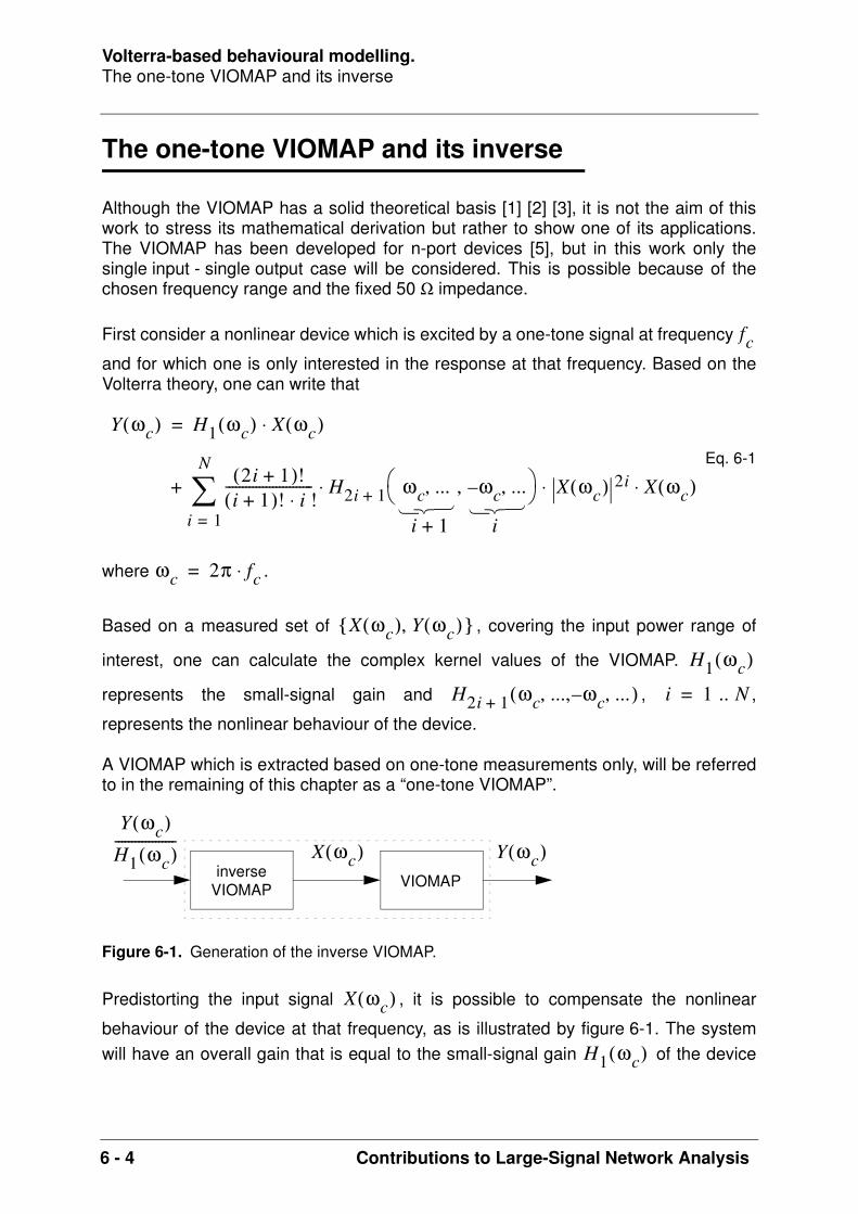
Volterra-based behavioural modelling.The one-tone VIOMAP and its inverse
6 - 4 Contributions to Large-Signal Network Analysis
The one-tone VIOMAP and its inverse
Although the VIOMAP has a solid theoretical basis [1] [2] [3], it is not the aim of thiswork to stress its mathematical derivation but rather to show one of its applications.The VIOMAP has been developed for n-port devices [5], but in this work only thesingle input - single output case will be considered. This is possible because of thechosen frequency range and the fixed 50 Ω impedance.
First consider a nonlinear device which is excited by a one-tone signal at frequency
and for which one is only interested in the response at that frequency. Based on theVolterra theory, one can write that
Eq. 6-1
where .
Based on a measured set of , covering the input power range of
interest, one can calculate the complex kernel values of the VIOMAP.
represents the small-signal gain and , ,
represents the nonlinear behaviour of the device.
A VIOMAP which is extracted based on one-tone measurements only, will be referredto in the remaining of this chapter as a “one-tone VIOMAP”.
Predistorting the input signal , it is possible to compensate the nonlinear
behaviour of the device at that frequency, as is illustrated by figure 6-1. The systemwill have an overall gain that is equal to the small-signal gain of the device
Figure 6-1. Generation of the inverse VIOMAP.
fc
Y ωc( ) H1 ωc( ) X ωc( )⋅=
2i 1+( )!i 1+( )! i !⋅
-------------------------- H2i 1+ ωc ..., ωc– ...,, X ωc( ) 2i⋅ ⋅
i 1=
N
X ωc( )⋅+
i 1+ i
ωc 2π fc⋅=
X ωc( ) Y ωc( ),
H1 ωc( )
H2i 1+ ωc ..., ω– c ...,,( ) i 1 .. N=
Y ωc( )H1 ωc( )------------------ X ωc( ) Y ωc( )
inverseVIOMAP VIOMAP
X ωc( )
H1 ωc( )
Volterra-based behavioural modelling.The one-tone VIOMAP and its inverse
Contributions to Large-Signal Network Analysis 6 - 5
under test, if for each measured output the corresponding input equals
. One can now generate a second data set starting from
the measured data set and use it to calculate the complex kernel
values of the “inverse VIOMAP”. It is important to notice that using this approach thebehaviour of the overall system will only be linearized for input powers in the power
range covered by , and not for the powers in the original range covered by
.
Y ωc( )
Y ωc( )H1 ωc( )------------------
Y ωc( )H1 ωc( )------------------ X ωc( ),
X ωc( ) Y ωc( ),
Y ωc( )H1 ωc( )------------------
X ωc( )

Volterra-based behavioural modelling.Predistortion of narrowband signals based on an inverse VIOMAP
6 - 6 Contributions to Large-Signal Network Analysis
Predistortion of narrowband signals based on an inverse VIOMAP
The one-tone VIOMAP, extracted based on measurements at the center frequency,can be extended to describe the response of weakly nonlinear systems to narrowbandsignals [6]. The verification of the validity of this “extrapolation” is one of the maintopics of this work and will be discussed in detail further on.
A narrowband band-pass signal can always be written as
. The function is called the envelope of and is
referred to as the phase modulation function. The corresponding output can be predicted based on the VIOMAP, measured
at , as is shown below. Using the complex notation, one finds
Eq. 6-2
In the case of IQ modulation, , such that
corresponds to and to
. This way, it is easy to understand how to
predistort and : if is changed to become
, then the response of the
system to the modulation is the desired modulated signal. Here,
represents the inverse VIOMAP, and represent the predistorted versions
of and , and .
x t( )a t( ) ωct φ t( )+( )cos⋅ a t( ) x t( ) φ t( )
y t( ) b t( ) ωct ψ t( )+( )cos⋅=
fc
Y ωc t,( ) 12--- b t( ) e
jψ t( )⋅ ⋅ H1 ωc( ) X ωc t,( )⋅= =
2i 1+( )!i 1+( )! i !⋅
-------------------------- H2i 1+ ωc .. ωc– .., , ,( ) X ωc t,( ) 2i X ωc t,( )⋅ ⋅ ⋅i 1=
N
+
X ωc t,( ) 12--- a t( ) ejφ t( )⋅ ⋅=
x t( ) i t( ) ωct( )cos⋅ q t( ) ωct( )sin⋅–=
i t( ) a t( ) φ t( )[ ]cos⋅ 2 re X ωc t,( )( )⋅= q t( )
a t( ) φ t( )[ ]sin⋅ 2 im X ωc t,( )( )⋅=
i t( ) q t( ) X ωc t,( ) 12--- i t( ) j q t( )⋅+[ ]⋅=
X' ωc t,( ) Hinv X ωc t,( )[ ] 12--- i' t( ) jq' t( )+[ ]⋅= =
i' t( ) jq' t( )+ Hinv
i' t( ) q' t( )i t( ) q t( ) j 1–=
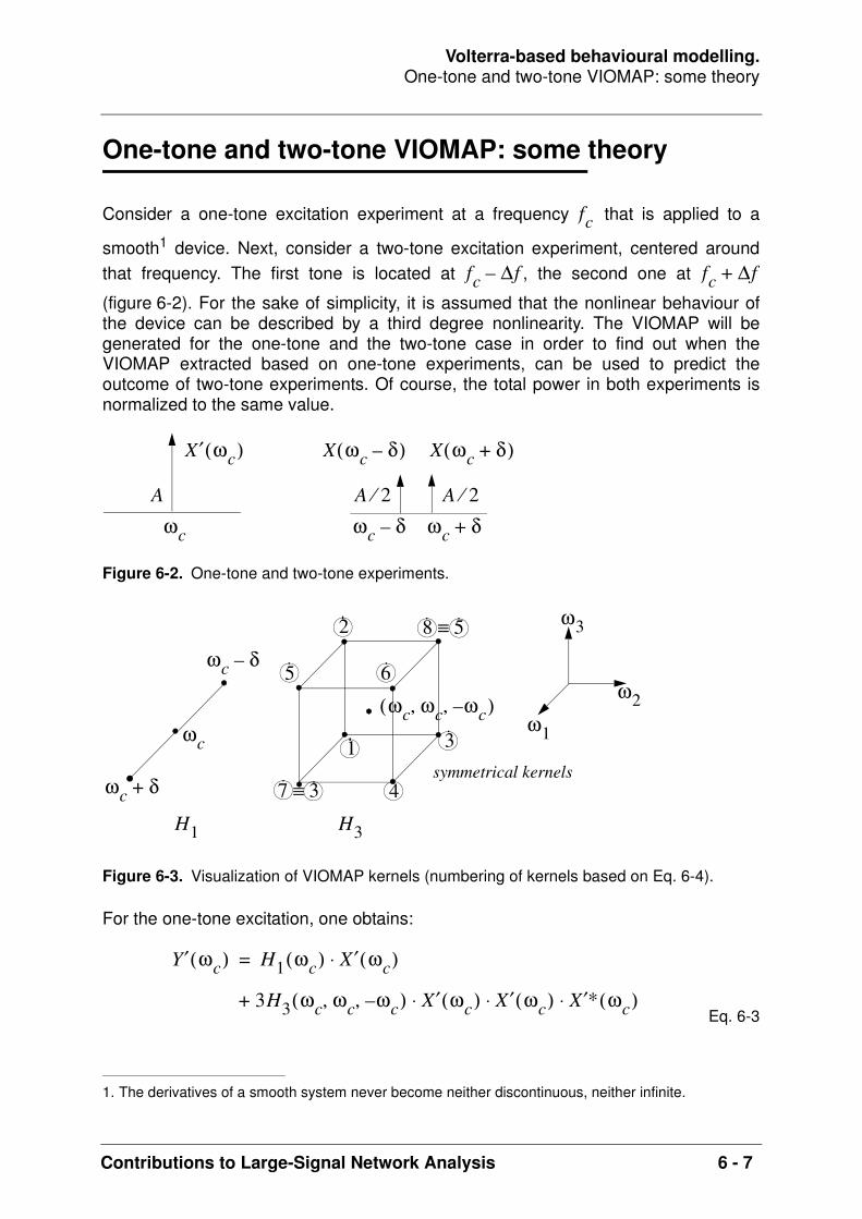
Volterra-based behavioural modelling.One-tone and two-tone VIOMAP: some theory
Contributions to Large-Signal Network Analysis 6 - 7
One-tone and two-tone VIOMAP: some theory
Consider a one-tone excitation experiment at a frequency that is applied to a
smooth1 device. Next, consider a two-tone excitation experiment, centered aroundthat frequency. The first tone is located at , the second one at
(figure 6-2). For the sake of simplicity, it is assumed that the nonlinear behaviour ofthe device can be described by a third degree nonlinearity. The VIOMAP will begenerated for the one-tone and the two-tone case in order to find out when theVIOMAP extracted based on one-tone experiments, can be used to predict theoutcome of two-tone experiments. Of course, the total power in both experiments isnormalized to the same value.
For the one-tone excitation, one obtains:
Eq. 6-3
1. The derivatives of a smooth system never become neither discontinuous, neither infinite.
Figure 6-2. One-tone and two-tone experiments.
Figure 6-3. Visualization of VIOMAP kernels (numbering of kernels based on Eq. 6-4).
fc
fc ∆f– fc ∆f+
A
X′ ωc( ) X ωc δ–( ) X ωc δ+( )
A 2⁄A 2⁄ωc δ– ωc δ+ωc
1
2
3
4
5 6
7 3≡
8 5≡
H1 H3
ω1
ωc δ+
ω2
ωc δ–
ω3
ωc
ωc ωc ωc–, ,( )
symmetrical kernels
Y′ ωc( ) H1 ωc( ) X′ ωc( )⋅=
3H3 ωc ωc ω– c, ,( ) X′ ωc( ) X′ ωc( ) X′∗ ωc( )⋅ ⋅ ⋅+

Volterra-based behavioural modelling.One-tone and two-tone VIOMAP: some theory
6 - 8 Contributions to Large-Signal Network Analysis
Let , and , then the response for the two-
tone experiment is:
Eq. 6-4
Now let to normalize the power for both experiments. One then
obtains:
Eq. 6-5
which is equal to Eq. 6-3.
Eq. 6-4 and figure 6-3 show under which conditions it becomes possible to use thekernels of the one-tone VIOMAP at a given center frequency to predict the output
in the case of two-tone measurements at the frequencies and . This
requires the monitoring of the variation of the complex kernels around in the th-dimensional space. Here
represents the degree of nonlinearity. The more constant these kernels remain in the
δ 2π∆f= ω+ ωc δ+= ω- ωc δ–=
Y ωc 3δ–( ) 3H3 ω- ω- ω+–, ,( ) X ω-( ) X ω-( ) X∗ ω+( )⋅ ⋅ ⋅=
3H3 ω- ω- ω-–, ,( ) X ω-( ) X ω-( ) X∗ ω-( )⋅ ⋅ ⋅+
Y ωc δ–( ) H1 ωc δ–( ) X ωc δ–( )⋅=
Y ωc δ+( ) H1 ωc δ+( ) X ωc δ+( )⋅=
6H3 ω- ω+ ω+–, ,( ) X ω-( ) X ω+( ) X∗ ω+( )⋅ ⋅ ⋅+
3H3 ω+ ω+ ω+–, ,( ) X ω+( ) X ω+( ) X∗ ω+( )⋅ ⋅ ⋅+
6H3 ω+ ω- ω-–, ,( ) X ω+( ) X ω-( ) X∗ ω-( )⋅ ⋅ ⋅+
Y ωc 3δ+( ) 3H3 ω+ ω+ ω-–, ,( ) X ω+( ) X ω+( ) X∗ ω-( )⋅ ⋅ ⋅=
Y ωc( ) 2H1 ωc( ) X ωc( )⋅=
24H3 ωc ωc ωc–, ,( ) X ωc( ) X ωc( ) X∗ ωc( )⋅ ⋅ ⋅+
δ 0→( )
1
2
4
3
5
6
X′ ωc( ) 2 X ωc( )⋅=
Y ωc( ) H1 ωc( ) X′ ωc( )⋅=
3H3 ωc ωc ω– c, ,( ) X′ ωc( ) X′ ωc( ) X′∗ ωc( )⋅ ⋅ ⋅+
fcfc ∆f– fc ∆f+
H2i 1+ ωc ... ωc ...,–, ,( ) 2i 1+( ) 2i 1+( )

Volterra-based behavioural modelling.One-tone and two-tone VIOMAP: some theory
Contributions to Large-Signal Network Analysis 6 - 9
neighbourhood of the point at coordinates , the better the prediction
of the spectral components at the output will be. Hence, this results in a quasi-statichypothesis.
Due to the ill-conditioned nature of power series approximations, verification based onconstant values of the VIOMAP kernels may turn out not to be a practically usablesolution. A much simpler and more practical approach is to take a look at the variationof the generated spectral components at the output, both in amplitude and in phase,based on two-tone measurements with constant input power and varying frequencyspacing. A concrete example of this approach can be found further on in this work.
ωc ... ωc ...,–, ,( )

Volterra-based behavioural modelling.Measurement setup and results
6 - 10 Contributions to Large-Signal Network Analysis
Measurement setup and results
Measurement setup
Figure 6-4 shows a simple communication link consisting of an IQ modulator, anamplifier and an IQ demodulator [8]. The distortion introduced by mixers will not beconsidered in this work, although it can be characterized using the VIOMAP modeltoo.
To demonstrate the use of the VIOMAP for narrowband signals, a measurement setup(figure 6-5) is realized where the modulator and demodulator are implemented insoftware and converted to real-word signals using an “arbitrary waveform generator”VXI card (HP/Agilent E1445A) and two “analog-to-digital convertor” VXI cards (HP/Agilent E1430A). A calibration process using a stepped sine wave is performed toeliminate the effect of the 10 MHz reconstruction filter of the arbitrary waveformgenerator (AWG) and the characteristics of the anti-aliasing filters at the inputs of the
Figure 6-4. A simple communication link.
Figure 6-5. The VXI-based measurement setup.
Φ2πfctcos
H
i(t)
q(t)
i’(t)
q’(t)
x(t)
y(t)90– ° 90– °
CostasLoop
Hx(t)
y(t)
-900
iin(t)
qin(t)
-900
iout(t)
qout(t)
-900
2πfctcosi(t)
q(t)
2πfctcos
2πfctcos
VXI
e1445a
40 MHz
reference clock: 40 MHz / 4
10 MHz
e1430a
e1430a channel 1
channel 2

Volterra-based behavioural modelling.Measurement setup and results
Contributions to Large-Signal Network Analysis 6 - 11
A/D convertors on the frequency grid of interest. The AWG runs at a samplingfrequency of 40 MHz and generates the 10 MHz master clock of the acquisition cardsputting a ‘0011’ marker sequence on the VXI backplane. The sequence which isdownloaded into the AWG is repeated continuously. At the end of each sequence a25 ns pulse is generated via the ‘Marker Out’ front panel connector and is used totrigger the acquisition cards, allowing repeated triggered measurements.
First the one-tone VIOMAP of the broadband (20 kHz - 2 GHz) Sonoma amplifier isdetermined using a sine wave excitation at the carrier frequency = 1.25 MHz. The
input power is swept from -26 dBm to -7 dBm. The linear (small-signal) gain of thisamplifier is found to be 20.75 dB. At an input power of -7 dBm this gain drops to19.15 dB, resulting in a gain compression of 1.6 dB. The corresponding phase shift of179.6 degrees is not sensitive to a change of the input power. In fact this is to beregretted, because the phase distortion is also described by the VIOMAP andtherefore can be corrected for by the inverse VIOMAP.
As will be explained later, also two-tone signals are generated in the close vicinity ofthe carrier frequency. Fixing the input power and sweeping the frequency spacingreveals subtle side effects.
A random sequence of 256 4-bit words is generated in software (figure 6-6). Thesymbol rate in set at 10 MHz / 256 = 39 kHz and 16QAM encoding is selected.Choosing powers of 2 for the record length allows the use of Fast Fourier Transformsto transform waveforms between the time domain and the frequency domain. In orderto keep the signals bandlimited, a raised-cosine filter [8] is used with a roll-off factor
= 0.5. This way, the bandwidth of the signal is limited to times the signal
rate, which results in 58.6 kHz. The filtered and are optionally predistortedby the inverse VIOMAP to compensate the nonlinear behaviour of the Sonomaamplifier. Finally these signals are modulated with a carrier frequency of 10 MHz /8 = 1.25 MHz. The resulting sequence is downloaded into the arbitrary waveform
generator and is continuously repeated. The 38.75 MHz alias component of thecarrier frequency is suppressed by the 10 MHz reconstruction filter. This is veryimportant when dealing with nonlinear devices. The maximum levels of the basebandsignals are scaled to correspond to an input power of -8.1 dBm, driving the amplifier
Figure 6-6. The generation of a (predistorted) 16QAM signal.
fc
raised cosine filter
i (t)
q (t) q’ (t)
i’ (t)random
sequenceof 256
4-bit symbols
16QAM
encoding
optionalpredistortion
based oninverse
VIOMAP
α = 0.5
1.25 MHz
+45º
-45º
RFout
α 1 α+( )i t( ) q t( )

Volterra-based behavioural modelling.Measurement setup and results
6 - 12 Contributions to Large-Signal Network Analysis
1.1 dB in compression. This input power must be covered by the VIOMAP in order toprevent extrapolation of the series approximation.
Model extraction.
A VIOMAP is extracted based on one-tone measurements at the carrier frequency,that cover an input power range of -26 dBm to -7 dBm. This one-tone VIOMAPcontains 6 complex parameters and describes the power of the
fundamental spectral component at the output as a function of the input power within0.01 dB. The maximum phase deviation is smaller than the measurement noise.Predistortion based on the corresponding inverse VIOMAP reduces the distortion ofthe constellation diagram and the corresponding spectral regrowth, but theimprovement is not as drastic as could be expected. Measurement of the constellationdiagram at the output reveals the presence of overcompensation.
To investigate the effect in more detail, a simple IQ signal is generated resulting in atwo-tone excitation of the amplifier. Choosing an appropriate baseband signal
the corresponding modulated signal
Figure 6-7. Measurement and prediction of iout(t) in the case of a simple IQ signal.
H1 H3 ..., H11, ,( )
-1.0
-0.8
-0.6
-0.4
-0.2
0.0
0.2
0.4
0.6
0.8
1.0
0 .1 .2
.90
.91
.92
.93
.09 .10 .11
measurementprediction based on one-tone VIOMAPprediction based on static two-tone VIOMAP (± 5 kHz)prediction based on static two-tone VIOMAP (± 30 kHz)
iin (t) = qin (t) = A.cos (2π.∆f.t)A = . 1 V
∆ f = 5 kHz
t (ms)
t (ms)
iout (t)
fc = 1.25 MHz
iout (t)
i t( ) q t( ) A 2π∆f t⋅( )cos⋅= = x t( )
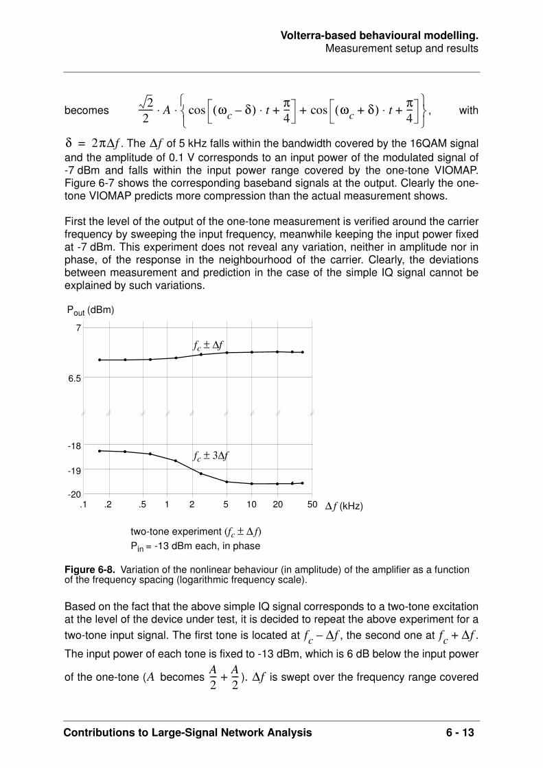
Volterra-based behavioural modelling.Measurement setup and results
Contributions to Large-Signal Network Analysis 6 - 13
becomes , with
. The of 5 kHz falls within the bandwidth covered by the 16QAM signaland the amplitude of 0.1 V corresponds to an input power of the modulated signal of-7 dBm and falls within the input power range covered by the one-tone VIOMAP.Figure 6-7 shows the corresponding baseband signals at the output. Clearly the one-tone VIOMAP predicts more compression than the actual measurement shows.
First the level of the output of the one-tone measurement is verified around the carrierfrequency by sweeping the input frequency, meanwhile keeping the input power fixedat -7 dBm. This experiment does not reveal any variation, neither in amplitude nor inphase, of the response in the neighbourhood of the carrier. Clearly, the deviationsbetween measurement and prediction in the case of the simple IQ signal cannot beexplained by such variations.
Based on the fact that the above simple IQ signal corresponds to a two-tone excitationat the level of the device under test, it is decided to repeat the above experiment for atwo-tone input signal. The first tone is located at , the second one at .
The input power of each tone is fixed to -13 dBm, which is 6 dB below the input power
of the one-tone ( becomes ). is swept over the frequency range covered
Figure 6-8. Variation of the nonlinear behaviour (in amplitude) of the amplifier as a function of the frequency spacing (logarithmic frequency scale).
22
------- A ωc δ–( ) t⋅ π4---+cos ωc δ+( ) t⋅ π
4---+cos+
⋅ ⋅
δ 2π∆f= ∆f
-20
-19
-18
6.5
7
.1 1 5 10 202 50.2 .5 ∆ f (kHz)
Pout (dBm)
fc ± ∆f
fc ± 3∆f
two-tone experiment (fc ± ∆ f)Pin = -13 dBm each, in phase
fc ∆f– fc ∆f+
A A2--- A
2---+ ∆f

Volterra-based behavioural modelling.Measurement setup and results
6 - 14 Contributions to Large-Signal Network Analysis
by the modulated 16QAM signal. This experiment clearly shows a variation of thenonlinear behaviour of the amplifier as a function of , as indicated by the variationof both amplitude (figure 6-8) and phase of the fundamental tones and their closestside lobes. Repeating the experiment at a carrier frequency of 1.23 MHz, which
corresponds to a of 20 kHz when using a carrier at 1.25 MHz, results in identicalplots. This way it is proven that the phenomenon is independent of small variations ofthe carrier frequency itself. The measurement of the linear gain of the amplifier at lowfrequencies (figure 6-9) reveals the presence of a transition zone starting at 10 kHz.This corresponds to twice the transition at a of 5 kHz in the case of the two-toneexperiment (figure 6-8). At that moment the frequency spacing of the two-tone equals10 kHz. Assuming that the low-pass characteristic of the DC bias circuit has acomparable bandwidth and that its cut-off frequency is larger than that of the ACcoupling of the Sonoma amplifier, the variation of the nonlinear behaviour can beexplained by the self-biasing effect of the amplifier which is mirrored around the carrierfrequency.
Under a one-tone excitation, the power of the RF input signal will determine the shift ofthe bias point, but it will only induce a shift in the DC bias settings. As soon as onemodulates the one-tone signal, the DC bias will try to track the modulation. Because aDC bias network is a low-pass circuit, it can’t always track the modulation immediately.Therefore, low-frequency voltages and currents are induced which reflect the low-frequent (LF) characteristics of the bias circuitry. This is referred to as (one possiblesource of) memory effects. Unfortunately, these effects get multiplied back to the RFsignal such that one can observe the LF behaviour in the modulation of the RF signal.This leads to different input-output characteristics depending on the test signal.
Figure 6-9. Linear gain of the broadband amplifier (Pin = -35 dBm).
∆f
fc∆f
∆f
-60
-50
-40
-30
-20
-10
0
10
20
0 10 20 30 40
gain (dB)
f (kHz)

Volterra-based behavioural modelling.Measurement setup and results
Contributions to Large-Signal Network Analysis 6 - 15
Static two-tone VIOMAP and its inverse.
Based on the two-tone measurement that reveals the variation of the nonlinearbehaviour of the amplifier as a function of the frequency spacing of the two-tone,a better model can be extracted to predict the response of the amplifier in the case ofthe 16QAM signal. Because the 16QAM signal uniformly covers a frequency range up
to a of 29.3 kHz, 83% (= ) of the signal is well described by a two-tone
measurement with a higher than 5 kHz. Therefore, a static VIOMAP is extracted
based on two-tone measurements with a of 30 kHz. The input power of each toneis raised from -32 dBm to -13 dBm. The individual input powers of each tone arecombined such that an equidistant two-dimensional grid is covered, each axiscorresponding to the input power of each tone, expressed in dBm. The VIOMAP ischosen to be static in order to map its kernels on the ones found
based on one-tone measurements at the carrier frequency. As such, these new kernelvalues are able to predict the outcome of the set of one-tone
experiments, which were used to generate the one-tone VIOMAP, thus creating a setof pairs. As expected, the resulting compression characteristic
Figure 6-10. Compression characteristic of the amplifier at 1.25 MHz (one-tone vs. two-tone).
prediction based on static two-tone VIOMAP (± 30 kHz)one-tone measurement
Pin (dBm) -5.0E+00-30.0E+00
-6.0
Pout(dBm)
14.0
Pin(dBm) -7.0E+00-10.0E+00
Pout(dBm)
10.0
12.5
2∆f
∆f 29.3 5–29.3
-------------------
∆f∆f
H1 H3 ..., H11, ,( )
Ypred ωc( )
X ωc( ) Ypred ωc( ),
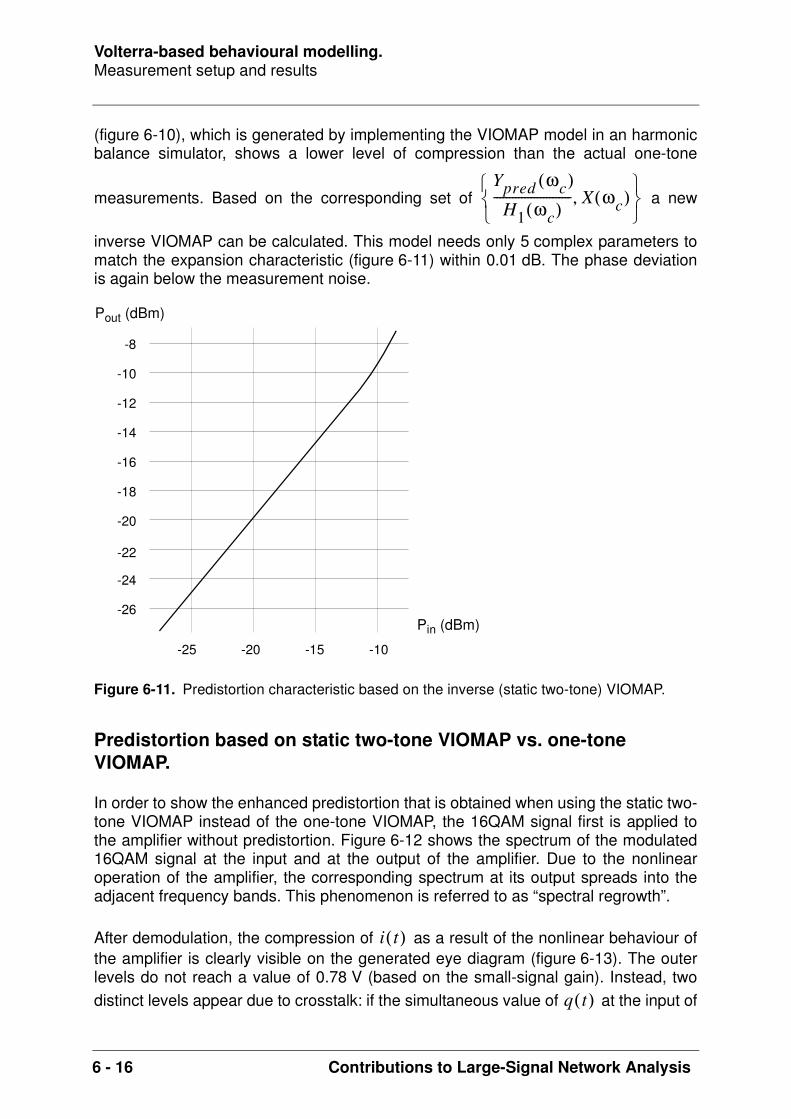
Volterra-based behavioural modelling.Measurement setup and results
6 - 16 Contributions to Large-Signal Network Analysis
(figure 6-10), which is generated by implementing the VIOMAP model in an harmonicbalance simulator, shows a lower level of compression than the actual one-tone
measurements. Based on the corresponding set of a new
inverse VIOMAP can be calculated. This model needs only 5 complex parameters tomatch the expansion characteristic (figure 6-11) within 0.01 dB. The phase deviationis again below the measurement noise.
Predistortion based on static two-tone VIOMAP vs. one-tone VIOMAP.
In order to show the enhanced predistortion that is obtained when using the static two-tone VIOMAP instead of the one-tone VIOMAP, the 16QAM signal first is applied tothe amplifier without predistortion. Figure 6-12 shows the spectrum of the modulated16QAM signal at the input and at the output of the amplifier. Due to the nonlinearoperation of the amplifier, the corresponding spectrum at its output spreads into theadjacent frequency bands. This phenomenon is referred to as “spectral regrowth”.
After demodulation, the compression of as a result of the nonlinear behaviour ofthe amplifier is clearly visible on the generated eye diagram (figure 6-13). The outerlevels do not reach a value of 0.78 V (based on the small-signal gain). Instead, twodistinct levels appear due to crosstalk: if the simultaneous value of at the input of
Figure 6-11. Predistortion characteristic based on the inverse (static two-tone) VIOMAP.
Ypred ωc( )H1 ωc( )
------------------------- X ωc( ),
-26
-24
-22
-20
-18
-16
-14
-12
-10
-8
-20 -10-25 -15
Pout (dBm)
Pin (dBm)
i t( )
q t( )

Volterra-based behavioural modelling.Measurement setup and results
Contributions to Large-Signal Network Analysis 6 - 17
the amplifier correspond to one of both outer levels too, the amplifier will be drivenmore into compression and the resulting at the output will be smaller than in the
case the value of at the input of the amplifier correspond to one of both innerlevels. This is clear when looking at the corresponding constellation diagram (figure 6-14).
It should be noted that figure 6-13 and figure 6-14 correspond to measurementsperformed as part of [6]. In that case, the outer levels should reach a value of 1.2 V(based on the small-signal gain). During the predistortion experiment, the maximumlevels of and have been reduced.
The effect of predistortion on the spectrum at the input of the amplifier is shown forboth the one-tone and two-tone VIOMAP (upper portion of figure 6-15) and theresulting spectrum at the output clearly shows the enhancement when thepredistortion is based on a static two-tone VIOMAP instead of a one-tone VIOMAP(lower portion of figure 6-15). The spectral regrowth is reduced an extra 10 dB,
Figure 6-12. Original 16QAM input (thin) and output (thick) spectrum.
-100
-90
-80
-70
-60
-50
-40
-30
-20
-10
Pin,out (dBm)
1.24 1.25 1.26 f (MHz)
-110
-120
-130
i t( )q t( )
i t( ) q t( )

Volterra-based behavioural modelling.Measurement setup and results
6 - 18 Contributions to Large-Signal Network Analysis
Figure 6-13. Measured eye diagram of i(t) at the output of the amplifier (no predistortion) for maximum levels of i(t) and q(t) at the input, which result in 2 dB compression. Two distinct levels become apparent at the indicated outer levels (circles) and even at the inner levels.
Figure 6-14. Measured constellation diagram at the output of the amplifier (no predistortion) for maximum levels of i(t) and q(t) at the input, which result in 2 dB compression.
-1.4
-1.2
-1.0
-0.8
-0.6
-0.4
-0.2
0
0.2
0.4
0.6
0 10 t (µs)
iout(t) (V)
20 30 40 50
0.8
1.0
1.2
1.4
-1.2
-1.0
-0.8
-0.6
-0.4
-0.2
0
0.2
0.4
0.6
qout(t) (V)
0.8
1.0
1.2
iout(t) (V)-1.2-0.8-0.400.40.81.2
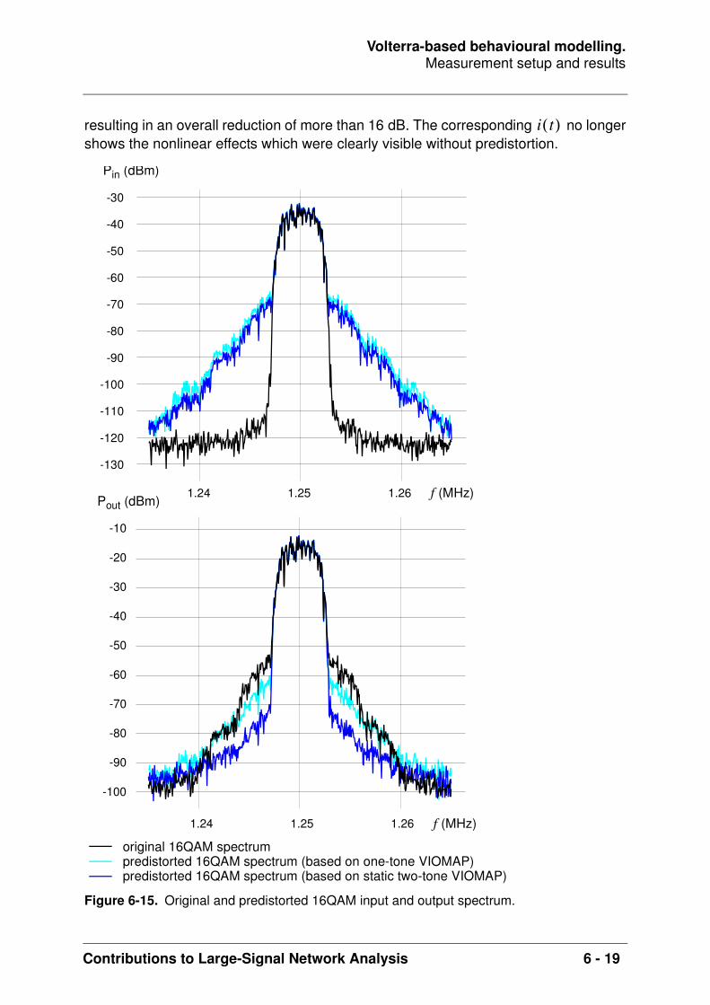
Volterra-based behavioural modelling.Measurement setup and results
Contributions to Large-Signal Network Analysis 6 - 19
resulting in an overall reduction of more than 16 dB. The corresponding no longershows the nonlinear effects which were clearly visible without predistortion.
Figure 6-15. Original and predistorted 16QAM input and output spectrum.
i t( )
-130
-120
-110
-100
-90
-80
-70
-60
-50
-40
-30
1.24 1.25 1.26
original 16QAM spectrumpredistorted 16QAM spectrum (based on one-tone VIOMAP)predistorted 16QAM spectrum (based on static two-tone VIOMAP)
f (MHz)
Pin (dBm)
-100
-90
-80
-70
-60
-50
-40
-30
-20
-10
1.24 1.25 1.26 f (MHz)
Pout (dBm)
Volterra-based behavioural modelling.Conclusions
6 - 20 Contributions to Large-Signal Network Analysis
Conclusions
It is shown that using an inverse VIOMAP, it is possible to enhance the linearity ofdigital communication channels. It is also demonstrated that one should be verycareful when extrapolating a nonlinear model that has been extracted at the carrierfrequency, to predict the response of the system to narrowband signals. Based onswept two-tone measurements one was able to explain the overcompensation whichshowed up during the 16QAM experiment when predistorting the baseband signalsusing an inverse VIOMAP based on measurements at the carrier frequency only. Atthe same time these measurements allowed the extraction of a better model resultingin an overall reduction of the spectral regrowth of more than 16 dB.
Volterra-based behavioural modelling.References
Contributions to Large-Signal Network Analysis 6 - 21
References
[1] M. Schetzen, “The Volterra and Wiener Theories of Nonlinear Systems”, Robert E.Krieger Publishing Company, 1989[2] W.J. Rugh, “Nonlinear System Theory. The Volterra/Wiener Approach”, John Hop-kins University Press, 1981[3] M. Vanden Bossche, “Measuring Nonlinear Systems. A Black Box Approach forInstrument Implementation”, Doctoral Dissertation, Vrije Universiteit Brussel, May1990[4] F. Verbeyst and M. Vanden Bossche, “The Volterra Input-Output Map of a HighFrequency Amplifier as a Practical Alternative to Load-Pull Measurements”, publishedin the Conference Proceedings of IMTC/94 and published in the Special Issue onSelected Papers IMTC/94 of the IEEE Transactions on Instrumentation and Measure-ment, vol. 44, no. 3, June 1995, pp 662 - 665.[5] F. Verbeyst and M. Vanden Bossche, “VIOMAP, the S-parameter equivalent forweakly nonlinear RF and microwave devices”, published in the Microwave Sympo-sium Digest of IEEE 1994 MTT-S International and published in the 1994 SpecialSymposium Issue of the MTT Transactions, vol. 42, no. 12, pp. 2531 - 2535.[6] F. Verbeyst, J. Verspecht and M. Vanden Bossche, “VIOMAP, a Way to Predict theDistortion of a Constellation Diagram due to Amplifier Nonlinearities”, published in theDigest of IEEE MTT-S European Topical Congress, Technologies for Wireless Appli-cations, Turin, November 1994.[7] F. Verbeyst and M. Vanden Bossche, “VIOMAP, 16QAM and Spectral Regrowth:Enhanced Prediction and Predistortion based on Two-Tone Black-Box Model Extrac-tion”, published in the Proceedings of the 45th ARFTG Conference, Orlando, June1995 and winner of the “Best Conference Paper Award”.[8] K. Feher, “Digital Communication. Satellite/Earth Station Engineering”, Prentice-Hall, 1983.

Volterra-based behavioural modelling.References
6 - 22 Contributions to Large-Signal Network Analysis

Contributions to Large-Signal Network Analysis i
“Large-Signal Network Analysis” is still in its infancy. The work presented here arehumble contributions. Nevertheless it is believed that they represent a meaningfulcontribution to a growing community in a world where nonlinearities can no longer beignored.
The LSNA hardware abstraction layer was conceived more than 10 years ago andsurvived the replacement of several major hardware components without causing anyfrustration neither to the conceiver nor to its users. It is still used today at differentlocations worldwide. A few years ago, Microsoft launched its .NET1 initiative. Thepromise is that each of us can select the programming language we feel mostcomfortable with, as long as it targets the CLR2. It resulted in a new language calledC#3. It is an attempt to take the best of C++ and Java. I believe languages like C, C++and even Fortran remain key to the scientific community. Nevertheless, researchersshould keep an eye on this new evolution, especially when they have the ambition toallow as many people as possible to use their work “as is”. I’m convinced that newversions of the LSNA hardware abstraction layer should be “.NET aware”, either bydirectly targeting the .NET platform or by using the interoperability provided byMicrosoft between .NET managed code and native unmanaged code. Anotherevolution is driven by the multiple-core processors which were recently released bycompanies like Intel. Microsoft is working on concepts which should alleviate the painfor those who want to take advantage of multi-threaded programming.
The streamlined and enhanced implementation of the nose-to-nose calibrationtechnique and its application as a part of the calibration of the Large-Signal NetworkAnalyzer and the Lightwave Component Analyzer have served the community welland still does. The involvement of institutes like NIST was and remains essential toshow to the community that good calibration techniques are key components to obtaingood measurements. Furthermore, it fuelled the research at NIST related to theelectro-optic sampling system to become an alternative to the nose-to-nosecalibration technique. It also pushes the upper frequency limit at which calibratedLSNA measurements are possible. I’m convinced that it remains crucial to haveindependent techniques and as such I welcome further efforts, both with respect tonose-to-nose and EOS-based calibration techniques. Work has been performed atNIST (Technical Note 1528 by K. Remley) explaining the impact of the internalsampling circuitry on the phase error of the nose-to-nose calibration. This work andthe work reported by J. Scott, as referenced in the “Comparison of the nose-to-noseand EOS-based calibration technique“ chapter can serve as a starting point toimprove the actual nose-to-nose calibration further. To convince the sceptics amongst
1. pronounced as “dot NET”2. Common Language Runtime3. pronounced as “C sharp”
Conclusions and ideas for further research

Conclusions and ideas for further research
ii Contributions to Large-Signal Network Analysis
us, it may help to set up a comparison between the results obtained at NIST and thosebased on other electro-optic sampling systems. Clever researchers may come up witha third method that allows broad-band calibration. One challenge is to push the upperfrequency limit, increasing the frequency resolution of the phase calibration is another,as it is a key component to accurate large-signal measurements under modulatedexcitation. Therefore, I warmly welcome the recent efforts at the department and lookforward to the fruits of this work.
Many high-frequency sampling oscilloscopes still suffer from time base imperfections,namely distortion, drift and jitter. To my knowledge, the system identificationtechniques which are applied to enhance both jitter and drift estimation embody thefirst work which tackles the effects of both jitter and drift simultaneously. Although theresults can stand the comparison with other state-of-the-art techniques, it is expectedthat even better results can be obtained by combining the results of the chapter onjitter and drift estimation. Ideally, all time base effects should be consideredsimultaneously and correctly dealt with. Researchers, who feel challenged, may learnfrom a method1 which was recently reported by people at NIST and theimplementation is made available to others. A drawback of this approach is that itrequires the measurement of two quadrature sinusoids performed simultaneously withthe waveform of interest.
Simulations and designs rely on good models. The potential of Volterra-based modelshas been demonstrated through several applications. It is essential for practisingengineers to understand that omnipotent models which truthfully describe thenonlinear behaviour of their components under all possible large-signal conditionssimply don’t exist. One of the major goals of the early work on predistortion is to showthe potential pitfalls when using a model which is extracted using one class ofexcitation signals to predict the output of the system when applying another class ofexcitation signals. Predistortion based on such a model has the effect of a magnifying-glass. There is a strong need for additional research on measurement-basedbehavioural models. Researchers should “sell” new contributions by demonstratingtheir potential, without being tempted to “oversell” their models. I strongly believe thatthe use of random multi-sines will provide new insights in the analysis and modellingof large-signal behaviour. The major challenge there is to build a strong case todefend it in front of a potentially biased jury.
I believe that the research community has the difficult but challenging mission to push“Large-Signal Network Analysis” forward, without forgetting the poor souls out there,doing their best based on their present knowledge and experience. A balanced mix offundamental research, education and carefully chosen applications which “speak thelanguage” of the practising community is key to make “Large-Signal NetworkAnalysis” a success for all of us.
1. “Compensation of Random and Systematic Timing Errors in Sampling Oscilloscopes”, submitted for publication in the IEEE Transactions on Instrumentation and Measurement.A copy of the revised version which was submitted to IEEE and the software can be downloaded from http://www.boulder.nist.gov/div815/HSM_Project/Software.htm

Contributions to Large-Signal Network Analysis iii
Publications
PublicationsInternational periodicals
iv Contributions to Large-Signal Network Analysis
International periodicals
[1] Frans Verbeyst, M. Vanden Bossche, “Speed up power amplifier design by fastsource-pull, real-time load-pull and accurate measurement-based behaviouralmodels”, Microwave Engineering Europe - Editorial, November 2005, pp. 24-30 andMaury Microwave Application Note 5C-077
[2] J. Scott, J. Verspecht, B. Behnia, M. Vanden Bossche, A. Cognata, F. Verbeyst, M.Thorn, D. Scherrer, “Enhanced on-wafer time-domain waveform measurementthrough removal of interconnect dispersion and measurement instrument jitter”, IEEETransactions on Microwave Theory and Techniques, Vol. 50, No. 12, pp. 3022-28,December 2002
[3] F. Verbeyst, M. Vanden Bossche, “The Volterra Input-Output Map of a High-Frequency Amplifier as a Practical Alternative to Load-Pull Measurements”, IEEETransactions on Instrumentation and Measurement, Vol. 44, No. 3, pp. 662-65, June1995
[4] F. Verbeyst, M. Vanden Bossche, “VIOMAP, the S-parameter equivalent for weaklynonlinear RF and microwave devices”, Special Symposium Issue of IEEETransactions on Microwave Theory and Techniques, Vol. 42, No. 12, pp. 2531-35,December 1994
[5] R. Pintelon, P. Guillaume, Y. Rolain, F. Verbeyst, “Identification of linear systemscaptured in a feedback loop”, IEEE Transactions on Instrumentation andMeasurement, Vol. 41, No. 6, pp. 747-54, December 1992

PublicationsNational periodicals
Contributions to Large-Signal Network Analysis v
National periodicals
[6] F. Verbeyst, E. Vandamme, “Large-signal network analysis. Overview of themeasurement capabilities of a large-signal network analyzer”, Revue HF, No. 4,pp. 57-66, 2002
[7] F. Verbeyst, M. Vanden Bossche, “VIOMAP, 16QAM and spectral regrowth:enhanced prediction and predistortion based on two-tone black-box model extraction”,Revue HF, No. 2 : pp. 25-34, 1996

PublicationsConference papers
vi Contributions to Large-Signal Network Analysis
Conference papers
[8] L. Gommé, A. Barel, Y. Rolain, F. Verbeyst, “Fine frequency grid phase calibrationsetup for the Large Signal Network Analyzer”, Proceedings of the IEEE MTT-SInternational Microwave Symposium, MTT ‘06, June 2006, San Francisco, CA, USA
[9] F. Verbeyst, Y. Rolain, J. Schoukens, R. Pintelon, “System Identification ApproachApplied to Jitter Estimation”, IMTC Conference Proceedings, pp. 1752-57, winner of a"Honorable mention recognized by the Award Commission of Agilent Technologies",IMTC ‘06, April 2006, Sorrento, Italy
[10] F. Verbeyst, M. Vanden Bossche, “Measurement-based Behavioral Model underMismatched Conditions, a new and easy approach for an accurate model”,Proceedings of the 35th European Microwave Conference, October 2005, Paris,France
[11] S. Myoung, X. Cui, D. Chaillot, P. Roblin, F. Verbeyst, M. Vanden Bossche, S.Doo and W. Dai, “Large-signal network analyzer with trigger for baseband & RFsystem characterization with application to K-modeling & output baseband modulationlinearization”, Proceedings of the 64th ARFTG Conference, pp. 189-95, December2004, Orlando, USA
[12] F. Verbeyst, M. Vanden Bossche, “Real-time and optimal PA characterizationspeeds up PA design”, Proceedings of the 34th European Microwave Conference,pp. 431-34, October 2004, Amsterdam, The Netherlands
[13] S. Vandenplas, J. Verspecht, F. Verbeyst, E. Vandamme, M. Vanden Bossche,“Calibration Issues for the Large-Signal Network Analyzer”, Proceedings of the 60thARFTG Conference, pp. 99-106, December 2002, Washington DC, USA
[14] G. Vandersteen, F. Verbeyst, P. Wambacq, S. Donnay, “High-frequency nonlinearamplifier model for the efficient evaluation of inband distortion under nonlinear load-pull conditions”, Proceedings of the 2002 Design, Automation and Test in EuropeConference, pp. 586-90, March 2002, Paris, France
[15] J. Scott, B. Behnia, M. Vanden Bossche, A. Cognata, J. Verspecht, F. Verbeyst,M. Thorn, D. Scherrer, “Removal of Cable and Connector Dispersion in Time-DomainWaveform Measurements on 40Gb Integrated Circuits”, Proceedings of the IEEEMTT-S International Microwave Symposium, MTT ‘02, Vol. 3, pp. 1669-72, June 2002,Seattle, USA
[16] J. Verspecht, F. Verbeyst, M. Vanden Bossche, “Network Analysis Beyond S-parameters: Characterizing and Modeling Component Behaviour under ModulatedLarge-Signal Operating Conditions”, Proceedings of the 56th ARFTG Conference,December 2000, Boulder, USA

PublicationsConference papers
Contributions to Large-Signal Network Analysis vii
[17] J. Verspecht, F. Verbeyst, M. Vanden Bossche, “Measurement based behavioralmodeling of components under modulated large-signal operating conditions”,Proceedings of the 30th European Conference on Wireless Technologies, pp. 167-70,October 2000, Paris, France
[18] J. Verspecht, F. Verbeyst, M. Vanden Bossche, “Network analysis beyond S-parameters: Characterizing and modeling component behaviour under modulatedlarge-signal operating conditions”, Proceedings of the 30th European MicrowaveConference, Vol.2, pp. 373-76, October 2000, Paris, France
[19] D. DeGroot, P. Hale, M. Vanden Bossche, F. Verbeyst, J. Verspecht, “Analysis ofInterconnection Networks and Mismatch in the Nose-to-Nose Calibration”,Proceedings of the 55th ARFTG Conference, pp. 116-21, winner of the "Best PosterPaper Award", June 2000, Boston, USA
[20] J. Verspecht, F. Verbeyst, M. Vanden Bossche, P. Van Esch, “System LevelSimulation Benefits from Frequency Domain Behavioral Models of Mixers andAmplifiers”, Proceedings of the 29th European Microwave Conference, Vol. 2, pp. 29-32, October 1999, Munich, Germany
[21] M. Vanden Bossche, F. Verbeyst, J. Verspecht, “The Three Musketeers of LargeSignal RF and Microwave Design - Measurement, Modeling and CAE”, Proceedingsof the 53rd ARFTG Conference, June 1999, Anaheim, USA
[22] J. Verspecht, M. Vanden Bossche, F. Verbeyst, “Characterizing ComponentsUnder Large Signal Excitation: Defining Sensible Large Signal S-Parameters'?!”,Proceedings of the 49th ARFTG Conference, pp. 109-17, June 1997, Denver, USA
[23] F. Verbeyst, “Using Orthogonal Polynomials as Alternative for VIOMAP to ModelHardly Nonlinear Devices”, Proceedings of the 47th ARFTG Conference, June 1996,San Francisco, USA
[24] F. Verbeyst, M. Vanden Bossche, “VIOMAP, 16QAM and Spectral Regrowth:Enhanced Prediction and Predistortion based on Two-Tone Black-Box ModelExtraction”, Proceedings of the 45th ARFTG Conference, and winner of the “BestConference Paper Award”, June 1995, Orlando, USA
[25] F. Verbeyst, M. Vanden Bossche, “Enhancing the Linearity of DigitalCommunication Channels Using IQ Predistortion Based Upon an Inverse VIOMAP”,IEEE MTT-S International Microwave Symposium, MTT ‘95, May 1995, Orlando, USA
[26] F. Verbeyst, J. Verspecht, M. Vanden Bossche, “VIOMAP, a Way to Predict theDistortion of a Constellation Diagram due to Amplifier Nonlinearities”, Proceedings ofthe IEEE MTT-S European Topical Congress, Technologies for Wireless Applications,pp. 81-85, November 1994, Turin, Italy
PublicationsConference papers
viii Contributions to Large-Signal Network Analysis
[27] F. Verbeyst, M. Vanden Bossche, “VIOMAP, the S-parameter equivalent forweakly nonlinear RF and microwave devices”, Proceedings of the IEEE MTT-SInternational Microwave Symposium, Vol. 3, pp. 1369-72, MTT ‘94, May 1994, SanDiego, USA
[28] F. Verbeyst, M. Vanden Bossche, “The Volterra input-output map of a highfrequency amplifier as a practical alternative to load-pull measurements”, Proceedingsof the IEEE Instrumentation and Measurement Technology Conference, Vol. 1,pp. 283-86, IMTC '94, May 1994, Hamamatsu, Japan
[29] R. Pintelon, P. Guillaume, Y. Rolain, F. Verbeyst, “Identification of linear systemscaptured in a feedback loop”, Proceedings of the IEEE Instrumentation andMeasurement Technology Conference, pp. 14-20, IMTC '92, New York, USA

Contributions to Large-Signal Network Analysis ix
“Method of and an arrangement for characterizing non-linear behavior of RF andmicrowave devices in a near matched environment.”
F. Verbeyst, J. VerspechtUS Patent Application Publication, No. US 2003/0057963 A1USA, March 2003
Patents

Patents
x Contributions to Large-Signal Network Analysis

Contributions to Large-Signal Network Analysis xi
[1] Best Conference Paper Award at the 45th ARFTG Conference for the paper:“VIOMAP, 16QAM and Spectral Regrowth: Enhanced Prediction and Predistortionbased on Two-Tone Black-Box Model Extraction” by F. Verbeyst and M. VandenBossche, Orlando, USA, June 1995.
[2] ARFTG Technology Award1 for the “Development of Large-Signal MeasurementTechnology”, Washington DC, USA, December 2002.
[3] IMTC 2006 Honorable Mention recognized by the Agilent Technologies AwardCommission for the paper: “System Identification Approach Applied to JitterEstimation” by F. Verbeyst, Y. Rolain, J. Schoukens and R. Pintelon, Sorrento, Italy,April 2006.
1. Recipients of the same award: M. Vanden Bossche and J. Verspecht.
Awards

Awards
xii Contributions to Large-Signal Network Analysis
Related Documents