Aalborg Universitet Modeling and control of large-signal stability in power electronic-based power systems Shakerighadi, Bahram Publication date: 2020 Document Version Publisher's PDF, also known as Version of record Link to publication from Aalborg University Citation for published version (APA): Shakerighadi, B. (2020). Modeling and control of large-signal stability in power electronic-based power systems. Aalborg Universitetsforlag. Ph.d.-serien for Det Ingeniør- og Naturvidenskabelige Fakultet, Aalborg Universitet General rights Copyright and moral rights for the publications made accessible in the public portal are retained by the authors and/or other copyright owners and it is a condition of accessing publications that users recognise and abide by the legal requirements associated with these rights. - Users may download and print one copy of any publication from the public portal for the purpose of private study or research. - You may not further distribute the material or use it for any profit-making activity or commercial gain - You may freely distribute the URL identifying the publication in the public portal - Take down policy If you believe that this document breaches copyright please contact us at [email protected] providing details, and we will remove access to the work immediately and investigate your claim. Downloaded from vbn.aau.dk on: April 03, 2022

Welcome message from author
This document is posted to help you gain knowledge. Please leave a comment to let me know what you think about it! Share it to your friends and learn new things together.
Transcript

Aalborg Universitet
Modeling and control of large-signal stability in power electronic-based power systems
Shakerighadi, Bahram
Publication date:2020
Document VersionPublisher's PDF, also known as Version of record
Link to publication from Aalborg University
Citation for published version (APA):Shakerighadi, B. (2020). Modeling and control of large-signal stability in power electronic-based power systems.Aalborg Universitetsforlag. Ph.d.-serien for Det Ingeniør- og Naturvidenskabelige Fakultet, Aalborg Universitet
General rightsCopyright and moral rights for the publications made accessible in the public portal are retained by the authors and/or other copyright ownersand it is a condition of accessing publications that users recognise and abide by the legal requirements associated with these rights.
- Users may download and print one copy of any publication from the public portal for the purpose of private study or research. - You may not further distribute the material or use it for any profit-making activity or commercial gain - You may freely distribute the URL identifying the publication in the public portal -
Take down policyIf you believe that this document breaches copyright please contact us at [email protected] providing details, and we will remove access tothe work immediately and investigate your claim.
Downloaded from vbn.aau.dk on: April 03, 2022


BA
HR
AM
SHA
KER
IGH
AD
IM
OD
ELING
AN
D C
ON
TRO
L OF LA
RG
E-SIGN
AL STA
BILITY
IN PO
WER
ELECTR
ON
IC-B
ASED
POW
ER SYSTEM
S
MODELING AND CONTROL OF LARGE-SIGNAL STABILITY IN POWER
ELECTRONIC-BASED POWER SYSTEMS
BYBAHRAM SHAKERIGHADI
DISSERTATION SUBMITTED 2020


Modeling and control of large-signal
stability in power electronic-based
power systems
by
Bahram Shakerighadi
Dissertation submitted July 24, 2020

Dissertation submitted: July 24, 2020
PhD supervisor: Prof. Frede Blaabjerg, Aalborg University
Assistant PhD supervisors: Prof. Claus Leth Bak, Aalborg University
Dr. Esmaeil Ebrahimzadeh, Ørsted Wind Power A/S, Fredericia, Denmark.
PhD committee: Professor Zhe Chen (chairman) Aalborg University
Professor JinJun Liu Xi’an Jiantong University
Professor Qing-Chang Zhong Illinois Institute of Technology
PhD Series: Faculty of Engineering and Science, Aalborg University
Department: Department of Energy Technology
ISSN (online): 2446-1636ISBN (online): 978-87-7210-679-3
Published by:Aalborg University PressKroghstræde 3DK – 9220 Aalborg ØPhone: +45 [email protected]
© Copyright: Bahram Shakerighadi
Printed in Denmark by Rosendahls, 2020

5
CV
{Bahram Shakerighadi} (SM’ 17) received the B.Sc. degree from University of
Mazandaran, Iran, in 2010 and the M.Sc. degree from University of Tehran, Iran, in
2014. He is currently working toward the Ph.D. degree in modeling and stability
assessment of the power-electronic-based power systems with Department of Energy
Technology, Aalborg University, Denmark.
He was also a Visiting Researcher with ABB Corporate Research, Västerås, Sweden.
His current research interests include modeling and stability assessment of Power
Electronic-based power systems, and control of grid-tied voltage source converters.


7
Abstract
Nowadays, power-electronic-based (PE-based) energy sources, such as wind turbines
and photovoltaics (PV), are increasing in capacity in electrical grids. Increasing the
penetration of PE-based energy sources in power systems changes the scope of
stability, security, reliability, and protection assessment of conventional power
systems. In modern power systems with a high penetration of PE-based energy
sources, the stability issues may lead to outage in a part of the system or even to a
blackout. Therefore, it is important to assess PE-based power systems stability
challenges to prevent undesired system outages in the grid.
In this project, it is tried to assess stability issues of modern power systems with the
focus on the large-signal stability challenges. The project starts with stability analysis
of grid-connected voltage source converters (VSCs), where different methods are used
to assess the stability of the grid-connected VSC. An energy function-based method
and an inertia-based method are used to analyze the stability of grid-tied VSC.
Besides, it is tried to assess the large-signal stability of the phase-locked loop (PLL)
as one of the most important control loops in most PE-based units.
Stability assessment of large-scale power systems with PE-based energy sources is
considered as the next step in this project. To do so, 4-machine Kundur and 23-
machine Nordic test systems are considered as the small-scale and the large-scale
power systems, respectively. The large-signal stability assessment is done to
demonstrate stability challenges of modern power systems with a high penetration of
PE-based energy sources. Thereafter, the large-signal stability challenges of modern
power systems is considered, where inertia-based assessment is used to analyze the
transient stability of PE-based power systems. The last part of this project gives a
solution to enhance the large-signal stability of modern power systems. Regarding the
large-signal stability assessment of PE-based power systems, it is concluded that the
distribution of PE-based energy sources affects the grid transient stability, and it can
be assessed based on the grid inertial response.


9
Dansk resume
Med en stigende andel af vedvarende energikilder som værende del af det moderne
elnet ændres omfanget af stabilitet, sikkerhed, pålidelighed og beskyttelses
evalueringen af det konventionelle elnet. I det moderne elnet, hvor der indgår en stor
andel effektelektronisk baseret energikilder kan stabilitetsproblemer lede til udfald af
generationsenheder og endda mørklægning af systemet. Derfor er det vigtigt at
evaluere stabilitets udfordringerne af det effektelektroniske baseret elnet for at undgå
uønsket effekter. I dette projekt evalueres stabilitets udfordringerne i elnettet med stor
fokus på modellering under større transiente forstyrrelser. Projektet indledes med
stabilitets analyse af netforbundet spændingskilde konvertere, hvor forskellige
metoder anvendes til at evaluere stabiliteten, der anvendes en metode baseret på en
energi-funktion og en metode baseret på en inerti-funktion. Derudover evalueres
stabiliteten ved større transiente forstyrrelser af fasesynkroniseringsenheden, som
udgør en af de vigtigste kontrolsløjfer i et effektelektronisk baseret elnet.
Stabilitets evaluering af stor-skala elnet som er baseret på vedvarende energikilder,
som værende det næste skridt i projektet, hvor to respektive elnet med henholdsvis 4
og 23 generationsenheder er taget i betragtning. Evalueringen af større transiente
forstyrrelser udføres for at påpege stabilitets udfordringerne ved elnet med en stor
andel af vedvarende energikilder. Efterfølgende er stabilitets udfordringerne under
større transiente forstyrrelser betragtet, hvor inerti-baseret evalueringer anvendes til
at analysere den transiente stabilitet. Under projektets afsluttende del fremføres en
løsning til at forbedre stabiliteten af det moderne elnet under større transiente
forstyrrelser. Med henblik på evalueringen af det moderne elnets stabilitet under større
transiente forstyrrelser, kan det konkluderes at fordelingen af vedvarende energikilder
har en indflydelse på den transiente stabilitet, og som kan evalueres på baggrund af
nettets inertielle respons.

MODELING AND CONTROL OF LARGE-SIGNAL STABILITY IN POWER ELECTRONIC-BASED POWER SYSTEMS
10

11
Table of contents
Abstract ...................................................................................................................... 7
Dansk resume ............................................................................................................ 9
Thesis Details ........................................................................................................... 13
Preface ...................................................................................................................... 16
Part I Report ........................................................................................................... 17
Chapter 1. Introduction .......................................................................................... 19
1.1. Background and Motivation .......................................................................... 19
1.2. Power System Stability ................................................................................. 24
1.3. Voltage Source Converters ........................................................................... 26
1.3.1. Classification of the Grid-Tied VSC ...................................................... 27
1.3.2. Stability Challenges of the Grid-Tied VSC ............................................ 33
1.4. Power-Electronic-based Power Systems ....................................................... 37
1.4.1. Stability Challenges of Modern Power Systems with High Penetration of
PE-based Units- Historical Review .................................................................. 38
1.4.2. PE-based Power Systems Stability Solutions ......................................... 39
1.5. Project Objectives and Limitation ................................................................. 40
1.5.1. Research Questions and Objectives ....................................................... 40
1.5.2. Project Limitations ................................................................................. 41
1.6. Thesis Outline ............................................................................................... 41
1.7. List of Publications ....................................................................................... 43
Chapter 2. Large-Signal stability and Control of grid-tied voltage source
converters................................................................................................................. 45
2.1. Abstract ......................................................................................................... 45
2.2. Background and motivation .......................................................................... 45
2.3. Large-signal Stability Assessment Techniques ............................................. 46
2.3.1. Fundamentals of Lyapunov Theory ....................................................... 46
2.3.2. Phase Portrait concept ............................................................................ 48
2.4. Grid-tied VSC’s component modelling ......................................................... 48
2.4.1. Current control loop ............................................................................... 49

MODELING AND CONTROL OF LARGE-SIGNAL STABILITY IN POWER ELECTRONIC-BASED POWER SYSTEMS
12
2.4.2. Delay caused by the PWM switching ..................................................... 50
2.4.3. SRF-PLL ................................................................................................ 50
2.5. Grid-tied VSC large-signal stability .............................................................. 51
2.5.1. Lyapunov- and Eigenvalue-based Stability Assessment of the Grid-
connected Voltage Source Converter ............................................................... 53
2.5.2. Large-Signal Stability Modeling for the Grid-Connected VSC Based on
the Lyapunov Method ...................................................................................... 64
2.5.3. Modeling and Adaptive Design of the SRF-PLL: Nonlinear Time-Varying
Framework ....................................................................................................... 70
2.6. Summary ....................................................................................................... 76
Chapter 3. Large-Signal stability and Control of Power-electronic-based power
systems ..................................................................................................................... 79
3.1. Abstract ......................................................................................................... 79
3.2. Background and motivation .......................................................................... 79
3.3. Inertial response of the grid-feeding power converters ................................. 94
3.4. Security Assessment of PE-based Power Systems ........................................ 79
3.5. Transient stability of power-electronic-based power systems ..................... 101
3.5.1. Simulation results ................................................................................. 105
3.6. Summary ..................................................................................................... 115
Chapter 4. Conclusion .......................................................................................... 117
4.1. Summary ..................................................................................................... 117
4.2. Thesis contributions .................................................................................... 118
4.3. Future Works............................................................................................... 119
References .............................................................................................................. 121
Part II Selected Publications ................................................................................ 132

13
Thesis Details
Thesis Title: Modeling and Control of Large-Signal Stability in Power
Electronic-based Power Systems
Ph.D. Student:
Bahram Shakerighadi
Supervisors:
Prof. Frede Blaabjerg
Prof. Claus Leth Bak
Dr. Esmaeil Ebrahimzadeh
The main body of the this thesis consists of the following papers:
Publications in Refereed Journals
J1. B. Shakerighadi, E. Ebrahimzadeh, F. Blaabjerg, and C. L. Bak, ‘‘Large-
signal stability modeling for the grid-connected VSC based on the
Lyapunov method,’’ in Energies, vol. 11, p. 2533, Oct. 2018.
J2. B. Shakerighadi, E. Ebrahimzadeh, M. G. Taul, F. Blaabjerg and C. L.
Bak, "Modeling and Adaptive Design of the SRF-PLL: Nonlinear Time-
Varying Framework," in IEEE Access, vol. 8, pp. 28635-28645, 2020.
J3. B. Shakerighadi, S. Peyghami, E. Ebrahimzadeh, M. G. Taul, F.
Blaabjerg and C. L. Bak, " A New Guideline for Security Assessment of
Power Systems with a High Penetration of Wind Turbines," in Appl. Sci.,
2020, 10, 3190.
Publications in Refereed Conferences
C1. B. Shakerighadi, E. Ebrahimzadeh, F. Blaabjerg and C. L. Bak,
"Lyapunov- and Eigenvalue-based Stability Assessment of the Grid-
connected Voltage Source Converter," 2018 IEEE International Power
Electronics and Application Conference and Exposition (PEAC),
Shenzhen, 2018, pp. 1-6.
C2. B. Shakerighadi, E. Ebrahimzadeh, C. L. Bak and F. Blaabjerg, " Large
Signal Stability Assessment of the Voltage Source Converter Connected

MODELING AND CONTROL OF LARGE-SIGNAL STABILITY IN POWER ELECTRONIC-BASED POWER SYSTEMS
14
to a Weak Grid," Proceedings of Cigre Symposium Aalborg 2019, 2019,
pp. 1-12.
C3. B. Shakerighadi, S. Peyghami, E. Ebrahimzadeh, F. Blaabjerg and C. L.
Bak, "Security Analysis of Power Electronic-based Power Systems,"
IECON 2019 - 45th Annual Conference of the IEEE Industrial Electronics
Society, Lisbon, Portugal, 2019, pp. 4933-4937.
C4. B. Shakerighadi, E. Ebrahimzadeh, F. Blaabjerg and C. L. Bak, "Large
Signal Stability Assessment of the Grid-Connected Converters based on
its Inertia," 2019 21st European Conference on Power Electronics and
Applications (EPE '19 ECCE Europe), Genova, Italy, 2019, pp. 1-7.
This dissertation has been submitted for assessment in partial fulfilment of the
Ph.D. degree. The thesis is a summary of the outcome from the Ph.D. project,
which is documented based on the above publications. Parts of the results are used
directly or indirectly in the extended summary of the thesis. The co-author
statements have been made available to the assessment committee and are also
available at the Faculty of Engineering and Science, Aalborg University.
Bahram Shakerighadi
Aalborg University, July 24, 2020

15

MODELING AND CONTROL OF LARGE-SIGNAL STABILITY IN POWER ELECTRONIC-BASED POWER SYSTEMS
16
Preface
This dissertation is a summary of the outcomes of the Ph.D. work entitled: “Modeling
and control of large-signal stability in power electronic-based power systems”, which
was carried out at the Department of Energy Technology, Aalborg University,
Denmark. The Aalborg University supports this Ph.D. project. The author would like
to give an acknowledgment to the above-mentioned institution.
Foremost, I would like to begin by expressing my sincere gratitude and appreciation
to my supervisor Professor Frede Blaabjerg, for his continuous guidance, motivation,
and patience throughout the entire Ph.D. study. His guidance helped me in all the time
of research and writing of this thesis. I would also like to extend my deepest gratitude
to my co-supervisors Professor Claus Leth Bak and Dr. Esmaeil Ebrahimzadeh for
their guidance and help during the entire period of the Ph.D. project. It has been such
a great experience to work under your supervision.
I am also grateful to Dr. Nicklas Johansson for providing me an opportunity to visit
ABB Corporate Research, Sweden, during my study abroad and broaden my
knowledge in the area of stability assessment of power-electronic-based power
systems.
Finally yet importantly, I would like to express my gratitude to my family for their
continuous support, encouragement and for always being there for me. None of this
would have been possible without you.
Bahram Shakerighadi
Aalborg University, July 24, 2020

17
Part I Report


19
Chapter 1.
Introduction
1.1. Background and Motivation
During the last decades, the structure of power systems has been changed from
conventional centralized systems with large-scale power generations to the modern
distributed ones with many smaller scale distributed generations (DGs) systems; see
Fig. 1.1 [1]. Most DGs are connected to the power systems by an inverter that makes
them power-electronic-based (PE-based) units [2]. Nowadays, modern power systems
with a high penetration of PE-based units, such as wind turbines and photovoltaics,
are facing different challenges regarding their stability, reliability, security,
protection, etc. [3]–[6].
The penetration of power PE-based energy sources, such as wind turbines and
photovoltaics, are increasing dramatically in power system grids as shown in Fig. 1.2.
By increasing the penetration level of PE-based units in power systems, different
stability challenges, such as harmonics, small-signal stability, and large- signal
stability, are changed [3], [7]. The main characteristics of the modern power systems
that distinguish them from the conventional ones are the following:
Fig. 1.1: Representation of a conventional power system (left). vs. a modern power electronic-based power system (right).
Centralized power
generation
End Users
Transmission
network
Conventional Power System
Centralized Oriented
Modern Power System with
Distributed Energy systems
End Users
Wind farms
Energy storage
PhotovoltaicsPower Electronic
Interface
End Users

MODELING AND CONTROL OF LARGE-SIGNAL STABILITY IN POWER ELECTRONIC-BASED POWER SYSTEMS
20
Modern power systems with a high penetration of PE-based units introduce
less inertial response in comparison with the conventional ones. This is due
to the lack of physical inertial response from PE-based units, such as wind
turbine and photovoltaics [7], [8].
PE-based units are synchronized with the rest of the system by using a
synchronization unit. This feature makes PE-based units distinguished from
the conventional energy sources, which are mostly based on the synchronous
generators (SGs). In SGs, the rotor’s speed is coupled with the system
frequency considering a swing equation relationship. In PE-based units, the
frequency is decoupled from the main grid, and a synchronization unit like
the phase-locked loop (PLL) is needed to measure the system
frequency/phase [9]. The frequency/phase measured by the PLL can be used
for the PE-based unit’s control system. However, its performance has a
strong impact on the stability of the system.
There are some limits for PE-based units operation, due to their sensitivity
to over-current and their ability to deal with the fault ride-through (FRT)
condition, e.g. in case of a short circuit in the grid. These limits lead to some
circumstances that make stability assessment of PE-based power system
different from the conventional one.
With all this in mind, system operators are facing grid challenges, e.g. the frequency
control under a high penetration of non-synchronous generation (NSG) [10].
Therefore, countries such as Ireland and U.K that have a relative small size and limited
interconnection with other grids, have introduced new services demand in order to
Fig. 1.2: Renewable energy generation in the world, 1965 to 2018 [11].

CHAPTER 1. INTRODUCTION
21
meet relevant challenges e.g. limited high rate-of-change-of-frequency (ROCOF)
(>0.5 Hz/s) [12]. For instance, a framework is designed to evaluate the system inertia
trend to indicate the risk of too high ROCOF in U.K. for a future “Go Green” scenario
[13].
Besides ROCOF, other frequency related challenges are introduced by the unbalance
between loads and generation in systems with a high penetration of NSG, which are
frequency response to large disturbances, voltage dip that leads to frequency dips,
frequency regulation and coping with its fluctuations, as well as over-frequency
generation shedding [10]. From a time-scale point of view, stability challenges
introduced in power grids can be categorized as it is shown in Fig. 1.3, where the
highlighted part indicates different stability challenges including both the small-signal
and large-signal stability phenomenon, and it is of interest in this project. The time-
scale related to the PE-based units control ranges from a few microseconds to several
milliseconds. Therefore, in can be said that the stability assessment of power-
electronic based power systems includes a wide range of time scale [14].
The topic of the small-signal stability assessment of PE-based power systems has been
well-studied in the literature [15]–[17]. The first step in small-signal stability analysis,
and generally in all stability studies, is to model the system in an appropriate way to
enable small-signal stability analysis [18].

MODELING AND CONTROL OF LARGE-SIGNAL STABILITY IN POWER ELECTRONIC-BASED POWER SYSTEMS
22
Fig. 1.3: Stability challenges and phenomenon in of power grids illustrated in terms of
time scale [19].
In small-signal stability analysis, it is tried to linearize the power system equations.
This makes the system model arranged in a way that it can be assessed by linear
stability analysis techniques [20]. Regarding techniques for small-signal stability
analysis, bode plot, eigenvalue analysis, and Nyquist criterion are straightforward to
use and here most of the controllers are designed based on that. However, it might be
a challenging issue to use the aforementioned techniques for a large-scale power
system [21]. The small-signal stability may not be credible when the system is
subjected to a large disturbance, due to the linearization techniques which are used,
are not valid any more [22]. In order to analyze the stability of the PE-based power
systems (and generally complex nonlinear systems), large-signal stability assessment
techniques should be used [23]–[26].
Large-signal stability of power systems is defined as the power system ability to
maintain stable when it is subjected to a large disturbance [27]. In other words, when
a large disturbance such as the generation trip or a three-phase fault happens in the
system, different stability criteria should be studied, and if the system can maintain
within its stability boundaries, then it can be said that the system is stable from a large-
signal stability point of view. Generally, there are three main categories of stability
that should be checked for when a large disturbance happens in the system: rotor angle
stability, frequency stability, and voltage stability. Mostly, each of the aforementioned
stability categories is analyzed separately; however, large disturbances may cause two
or three of stability challenges, instantly [28]. Most often, the large-signal stability is
Lightning Propagation
Boiler/Long-Term
Dynamics
Voltage Stability
Power Flow
-710 -510-310 0.1 10 310 510
Switching Surges
Stator Transients and Sub-
synchronous Resonance
Transient Stability
Governor and Load
Frequency Control
Time (Seconds)

CHAPTER 1. INTRODUCTION
23
related to transient stability. A large-signal stability time frame is usually 3 to 5
seconds; however, it may be extended up to 10 to 20 seconds, e.g. for frequency
stability assessment of the large-scale power systems.
In order to assess the large-signal stability assessment methods of PE-based power
systems (and generally complex nonlinear systems), the nonlinear terms are not
linearized, which makes the assessment complicated. There are some concepts that
are used regarding the large-signal stability analysis of PE-based power systems, such
as the Lyapunov theory (energy function theory) and equal area criterion [29], [30].
The main challenge for large-signal stability assessment techniques that are based on
the Lyapunov function is that there is no straightforward method to define the energy
function of a system. Therefore, it is a challenge to define an appropriate Lyapunov
function that indicates system stability boundaries [22].
In order to assess the large-signal stability of PE-based power systems, the first step
is to model the system in an appropriate way (like in the small-signal stability
assessment). The modeling of the PE-based power system could be varied based on
the focus of the study. For instance, if the main focus of the study is the stability of
the PE-based unit, then the rest of the system can typically be modeled as a stiff
voltage source or a simple voltage source and an impedance [31], [32]. On the other
hand, if the main focus of the study is the stability of the power system rather than the
PE-based unit, then a simple model for the PE-based unit might be used [33], [34].
However, a detailed model of the grid including all its components’ models introduces
a more realistic behavior of the system. After modeling the system, the next step is to
design controllers based on the stability assessment. However, it should be noticed
that most often the small-signal stability assessment is used for tuning the controllers,
even for large-signal stability case studies, e.g. in FRT case study [35], [36].
The large-signal stability assessment becomes more important as the penetration of
non-synchronous generators (NSGs) are increasing in power systems. By increasing
the penetration of NSGs, the main system becomes more vulnerable to large
disturbances, due to NSGs’ lack of inertial response [37], [38]. In this way, the main
grid’s ability to control the system frequency and bus voltage magnitude become less
compared to the stiff grid. Grids with less ability to control the system variables, such
as voltage magnitude of buses and the system frequency, are called weak grids [39]–
[41]. This definition of the weak grid is translated to “a voltage source connected to a
large impedance” in grid-tied VSC stability assessment [40], or a large-scale power
system with a low inertial response [42]. In some cases, the increase of NSG
penetration in power systems may even lead to blackouts.
In this project, the stability assessment methods of PE-based power systems are
studied. What is mainly motivates the author to focus on this topic is that renewable
energy sources (RESs) inevitably increase the penetration in power systems, and most
of them are connected via a PE interface, called an inverter. The literature regarding

MODELING AND CONTROL OF LARGE-SIGNAL STABILITY IN POWER ELECTRONIC-BASED POWER SYSTEMS
24
the modeling and stability assessment of such systems are mainly focusing on the
small-signal stability. However, small-signal stability analysis is not accurate in case
of a large-disturbance. Therefore, in this project, it is tried to introduce an insight
regarding the large-signal stability analysis of modern power systems.
1.2. Power System Stability
Power system stability has been a challenging issue for electrical grids for many
decades [27]. The stability assessment of power systems has been studied extensively
in the literature. The stability of power systems is categorized into three main topics
as discussed before: rotor angle stability, frequency stability, and voltage stability, as
shown in Fig. 1.4. All of the three categories of the power systems stability are divided
into some subcategories based on their causes (disturbance size) and their time scale
[43].
Fig. 1.4: Classical power system stability classification [27].
Most of the large disturbances in power systems, such as a three-phase short circuit
fault, lead to short-term instabilities, which is a 3-5 s time scale phenomenon in order
to recover [27]. However, the system scale might be affected by the time scale of an
Power
Systems
Stability
Rotor Angle
Stability
Frequency
Stability
Voltage
Stability
Small-
disturbance
Angle
Stability
Transient
Stability
Large-
disturbance
Voltage
Stability
Small-
disturbance
Voltage
Stability
Short term
Short term
Long term
Long term
Short term
CHAPTER 1. INTRODUCTION
25
event. For instance, the period for transient stability may be extended to 10-20 s for
very large-scale power systems.
In PE-based units, there is no physical rotational part that is synchronized with the
rest of the grid. This makes the rotor angle stability out of scope for the PE-based
units’ stability studies. On the other hand, PE-based units are coupled to the rest of
the system from the frequency point of view, as it is utilizing an inverter. Most often,
a PLL is used for the synchronization of a PE-based unit and the rest of the system.
To study the frequency stability of the PE-based units, the impact of PLL on its
stability should be considered as an important part. In this way, the frequency stability
of PE-based power systems is different from the conventional one. For power systems
with a high penetration of NSGs, the stability definition should be slightly different
from its definition for the conventional one or should be an expanded version of it.
A general guideline of PE-based power systems stability definition is discussed in
[44]. Although this guideline is developed for Microgrids, its definition can be used
for different PE-based power systems. It should be noticed that to apply such a
guideline to large-scale power systems with a high penetration of NSGs, the relevant
grid codes should be considered as well [45], [46]. As mentioned earlier, there is no
rotational part in PE-based units. Therefore, only the voltage stability and the
frequency stability are considered for PE-based units. However, the PE-based power
systems will typically include both conventional and modern types of energy sources,
which means that the conventional synchronous generators are still used as a part of
the modern power systems. The new guideline for PE-based power systems stability
introduced in [44], is shown in Fig. 1.5, where it can be seen in that PE-based power
systems stability assessment is categorized more in details for the conventional
systems (due to the introduction of more stability phenomenon by PE-based units),
yet conventional stability subcategories, such as voltage stability, frequency stability,
and rotor angle stability (electric machine stability), are kept like in the former one
(PE-based power systems stability assessment). The disturbance size (large and small
disturbances) and the time frame of the event are still used for distinguishing the
different kinds of instability issues for the PE-based power systems, as well as for the
conventional power systems.

MODELING AND CONTROL OF LARGE-SIGNAL STABILITY IN POWER ELECTRONIC-BASED POWER SYSTEMS
26
Fig. 1.5: Power electronic-based power systems stability classification [44].
It should also be noticed that in small-scale PE-based power systems, the systems
variables (frequency and voltage) are strongly coupled [44]. The reason is that
resistance to inductance ratio (R/X) is higher in small-scale power systems compared
with the large-scale systems. This leads to a coupling between active and reactive
power that are typically decoupled in the conventional power systems [47]. Therefore,
an event that triggers the frequency instability may lead to the voltage instability as
well. However, by increasing the scale of the system (by decreasing R/X ratio), e.g.
in a large-scale power system such as in the Nordic-32 test system [48], the frequency
stability and the voltage stability phenomenon can be distinguished easier than the
small-scale ones [49].
Another issue regarding the PE-based power systems stability classification is the
control stability category, as also shown in Fig. 1.5. This category is related to the
control loops of the synchronous machines and NSGs, LCL filters (which are the
output filter of the converters), and PLLs. Poor controller tuning, PLL bandwidth,
system synchronization failure, harmonic instability, etc., may lead to system
instability caused by the control system of NSGs (inverters), which is going to be
discussed in the next paragraphs.
1.3. Voltage Source Converters
As it is mentioned before, one of the key components of PE-based power systems is
voltage source converters (VSCs), which is used for RESs that are connected to the
rest of the system via an interface, called the inverter. Although different control
strategies are defined for VSCs, which will be discussed in Section 1.3.1, the main
PE-based
Power
Systems
Stability
Power
Supply and
Balance
Stability
Control
Stability
Frequency
Stability
Voltage
Stability
Electric
Machine
Stability
Converter
Stability
Small
disturbance
Large
disturbance
Short term
Long term
Short term
Long term
Small
disturbance
Large
disturbance
System
Voltage
Stability
DC-Link
Voltage
Stability

CHAPTER 1. INTRODUCTION
27
application of the VSCs is to transfer the energy produced by the renewable source to
the power system having an appropriate voltage level and frequency. A single-phase
diagram of a grid-tied VSC is shown in Fig. 1.6. 𝑍𝑐 and 𝑍𝑔 are the VSC output filter
and the grid impedance, respectively. The main grid is presented as an infinite bus,
which is a stiff voltage source and grid impedance. Regarding the infinite bus used in
the main grid, it is assumed that ��𝑔 has a fixed magnitude and phase angle. PCC shown
in Fig. 1.6 indicates the point of common coupling. In general, VSCs are used in two
main modes: grid-tied mode and islanded mode [50]. The control systems of VSCs
are designed and are tuned based on their applications and operation modes.
VSCs are used in the islanded mode when there is a difficulty to be connected to the
main grid or due to some special circumstances [51], [52]. An application of islanded
mode of VSC could be a situation that a fault occurs in the system and a part of the
grid needs to work in an isolated mode. In this case, a part of the system will be
disconnected from the rest of the system, and then the separated part works
independently. Also, islanded mode of VSCs can be used in shipboard power systems
and also other autonomous systems [52]. However, most often, VSCs are operated in
their grid-tied mode in PE-based power systems.
1.3.1. Classification of the Grid-Tied VSC
Based on the specific application and the VSC’s configuration, there are four main
control structures of grid-tied VSCs: grid-forming, grid-feeding, current-source-based
grid-supporting, and voltage-source-based grid-supporting. The schematics of these
four categories are shown in Fig. 1.7. In Fig. 1.7(a), 𝐸∗ and 𝜔∗ are the voltage
magnitude and frequency references, respectively. By using 𝐸∗ and 𝜔∗, the reference
voltage, 𝐯∗, will be generated. In Fig. 1.7(b), 𝑃∗ and 𝑄∗ are the active and reactive
power references, respectively, which are used to generate the reference value for the
current, 𝐢∗. In Fig. 1.7(c) and In Fig. 1.7(d), 𝐸∗, 𝜔∗, 𝑃∗, and 𝑄∗ are used to indicate the
modified values for active (𝑃∗∗) and reactive (𝑄∗∗) power.
Fig. 1.6: A single-phase diagram of a grid-tied voltage source converter (VSC).
PE-based Unit
Infinite
bus cZ gZ
gv
Main Grid
PCCVoltage source
converter
MODELING AND CONTROL OF LARGE-SIGNAL STABILITY IN POWER ELECTRONIC-BASED POWER SYSTEMS
28
1.3.1.1 Grid-Forming Power Converters
The grid-forming power converters are designed and operated, so they represent a
voltage source; see Fig. 1.7(a). The main application of the grid-forming power
converters is to act like a synchronous machine. In this way, a grid-forming power
converter introduces a voltage magnitude and frequency at its point of common
coupling (PCC) with the rest of the grid. In the case of islanding mode for a part of
the grid in which there are only PE-based energy sources, at least one grid-forming
power converter is needed to form the system reference, so the other converters can
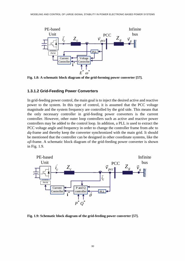
be synchronized with the grid-forming power converter. A schematic block diagram
of the grid-forming power converter is shown in Fig. 1.8.
Two of the main applications of grid-forming power converters is for energy storage
and uninterruptable power supplies (UPSs) [53]. What can be achieved from the grid-
forming power converters is also the ability to introduce inertial response [54].
The general from of the grid forming power converter is shown in Fig. 1.7(a), and the
grid-forming power converter model shown in Fig. 1.8 is just a kind of grid-forming
power converters. Any other control model for power converters that presents a
voltage source with a magnitude and the phase angle can be named a grid forming
power converter. In this regard, an interesting model implemented for the grid-
forming power converters is the virtual synchronous machine model (VSM) used for
the inverter control [55]. In the VSM model, it is tried to mimic the behavior of the
synchronous machine. The VSM control model of the VSC is to use it to control the
voltage magnitude and angle at the PCC and bring an inertial response to the active
power generation and consumption unbalance. The frequency of the VSC is coupled
into the VSM control. Controlling the PCC voltage angle is the same as controlling
the frequency. In this way, like in synchronous machines, if the system frequency
drops, the VSC injects more active power to compensate for the active power
consumption. This can be done by implementing the swing equation into the active
power control loop of the VSC. It is worth mentioning that in VSM control method,
there is no need to use a PLL to estimate the phase angle and the system frequency in
normal condition. However, the PLL might be used when the current limitation is
activated [56].

CHAPTER 1. INTRODUCTION
29
Fig. 1.7: Block-diagrams of grid-tied VSCs. (a) grid-forming, (b) grid-feeding, (c) current-source-based grid-supporting, and (d) voltage-source-based grid-supporting [57].
(d)
*P*Q
*
*E
cZ*v
vC
**
**EPC
QC
Infinite
bus gZ
Main Grid
PCC
(c)
cZPC*
i
**P
**QC
EC
*P
*Q
**E
Infinite
bus gZ
Main Grid
PCC
cZ
(b)
*P*Q PC
*i
Infinite
bus gZ
Main Grid
PCC
vC
**E
cZ*v
(a)
Infinite
bus gZ
Main Grid
PCC
MODELING AND CONTROL OF LARGE-SIGNAL STABILITY IN POWER ELECTRONIC-BASED POWER SYSTEMS
30
Fig. 1.8: A schematic block diagram of the grid-forming power converter [57].
1.3.1.2 Grid-Feeding Power Converters
In grid-feeding power control, the main goal is to inject the desired active and reactive
power to the system. In this type of control, it is assumed that the PCC voltage
magnitude and the system frequency are controlled by the grid side. This means that
the only necessary controller in grid-feeding power converters is the current
controller. However, other outer loop controllers such as active and reactive power
controllers may be added to the control loop. In addition, a PLL is used to extract the
PCC voltage angle and frequency in order to change the controller frame from abc to
dq-frame and thereby keep the converter synchronized with the main grid. It should
be mentioned that the controller can be designed in other coordinate systems, like the
αβ-frame. A schematic block diagram of the grid-feeding power converter is shown
in Fig. 1.9.
Fig. 1.9: Schematic block diagram of the grid-feeding power converter [57].
PE-based
Unit
PWM
PLL
Current
Controller
Infinite
bus
pccvci cZ gZ
gv
P and Q
controller*
i
PCC
ci
*P *Q
PE-based
Unit
PWMPLL
Current
Controller
Infinite
bus
pccvci cZ gZ
gv
Voltage
Controller
**E
*i
PCC

CHAPTER 1. INTRODUCTION
31
In grid-feeding power converters, it is assumed that the voltage and frequency of the
PCC is controlled by the main grid side. The problem with the grid-feeding power
converters is that when the number of grid-feeding power converters increases in the
power system, the main system becomes weaker, and a weak grid is less able to
control the system variables compared with a stiff grid. In this way, as the grid-feeding
power converters control relies on the system stiffness, the VSC in grid-feeding
control mode may become out of synchronization when it is connected to a weak grid
[58].
1.3.1.3 Current-source-based grid-supporting
This type of controller of the VSC is very similar to the grid-feeding power converter
control. The main goal is to inject active and reactive power assuming that the main
grid controls the PCC voltage magnitude, voltage phase, and the system frequency.
The difference between the current-source-based grid-supporting and the grid-feeding
power converter is the droop control introduced in the current-source-based grid
supporting converters. This is shown in Fig. 1.10.
Fig. 1.10: Schematic block diagram of the current-source-based grid-supporting power converter with additional droop control [57].
In this way, it can be said that the current-source-based grid-supporting control model
is an advanced version of the grid-feeding control model for the power converter.
1.3.1.4 Voltage-source-based grid-supporting
The voltage-source-based grid-supporting control mode of power converters is the
modified version of the grid-forming power converters. An outer control loop for the
active and reactive power is added to the grid-forming power converters controller, as
shown in Fig. 1.11.
PE-based
Unit
PWM
PLL
Current
Controller
Infinite
bus
pccvci cZ gZ
gv
P and Q
controller*
i
PCC
ci
Droop
control
*E * *P *Q
**Q
**P

MODELING AND CONTROL OF LARGE-SIGNAL STABILITY IN POWER ELECTRONIC-BASED POWER SYSTEMS
32
In this way, voltage-source-based grid-supporting power converters act similar to a
synchronous generator [55]. In this control scheme, the active and reactive power
injected into the system is dependent on the PCC voltage, pccv , the grid side
impedance, and the grid voltage [59]. In respect to the active and reactive power
control, the idea of the droop control can be used in order to mimic the behavior of a
synchronous generator. By using the droop control for the active and reactive power
regulation, the active power delivered to the system decreases when the grid frequency
increases, and also the reactive power decreases when the PCC voltage increases [57].
By increasing the penetration of PE-based energy sources in the power system, the
frequency stability will be supported due to the inertial support of the voltage-source-
based grid-supporting power converters.
Fig. 1.11: Schematic block diagram of the voltage-source-based grid-supporting power converter [57].
1.3.1.5 The use of different grid-tied VSC in power systems
Based on the system requirement and the capability of the PE-based energy sources,
each control method mentioned earlier has some applications. The grid-feeding power
converters are used to set the active and reactive power reference, so e.g. the
maximum power point tracking (MPPT) algorithms can be implemented for different
energy sources, e.g. photovoltaics and wind turbines [60].
Grid-supporting converters may introduce different services, such as the frequency
support and reactive power injection both in normal operation and during a fault, to
the system. Compared with the conventional synchronous generator, the grid-
supporting converters are able to act faster. However, it should be noticed that the
grid-supporting converters’ performance are very dependent on their energy source
type and size [57], [61].
PE-based
Unit
PWM
PLL
Current
Controller
Infinite
bus
pccvci cZ gZ
gv
P and Q
controller*
i
PCC
ci
Droop
controlVoltage
Controller
**P
**Q
*Q*P**E
*v

CHAPTER 1. INTRODUCTION
33
It seems that the future of the power grids is dependent on how to control the PE-
based energy sources as the grid-forming power converter, and the increasing of the
penetration of grid-feeding power converters may cause stability issues for the grid
[53]. In this way, power converters should be able to support the system with damping
power oscillations in addition to the voltage and frequency regulation [62]. Power
converters should also be able to provide black-start services for the grid [57]. For
this, a general guideline for using the NSGs in power systems is provided in [63].
1.3.2. Stability Challenges of the Grid-Tied VSC
In this part, it is tried to discuss different stability challenges introduced by the grid-
tied VSC for the power systems. To do so, the impact of grid-tied VSC on the different
systems stability categories and the grid-tied VSC stability challenges are discussed.
1.3.2.1 Grid-tied VSC Stability: Small-signal stability challenges
Considering the modeling of the grid-tied VSC, different stability challenges, such as
the PWM delay impact, tuning the PLL, and the grid stiffness (stiff grid or weak grid),
are contributions to some of the grid-tied VSC stability issues. In this part, the
importance of different stability challenges introduced by the control system of the
VSC with the grid-feeding control configuration is discussed. A more detailed
discussion is done in Chapter 2. In order to do so, small-signal stability is an important
issue. To assess the small-signal stability of the grid-tied VSC, an s-domain model of
the controller and the system can be used. An example of the grid-feeding VSC model
in the s-domain with a current and active power controller like shown in Fig. 1.12(a).
Besides, the small-signal model of the PLL is shown in Fig. 1.12 (b). It should be
noticed that the PCC voltage and the VSC output current are ��𝑐 = 𝑣𝑑 + 𝑣𝑞𝑗 and 𝑖𝑐 =
𝑖𝑑 + 𝑖𝑞𝑗, respectively, while the reference values for the PCC voltage and the VSC
output current are ��𝑐∗
= 𝑣𝑑∗ + 𝑣𝑞
∗𝑗 and 𝑖𝑐∗
= 𝑖𝑑∗ + 𝑖𝑞
∗𝑗, respectively.
In this model, the delay caused by the pulse-width modulation (PWM) is presented by
its Padé approximation [64]. The PWM delay model equals 𝑒−𝑇𝑑𝑠, where 𝑇𝑑 is the
time delay introduced by the switching; however, this is a non-linear term. To present
the delay in the small-signal stability model, the Padé approximation of the delay is
presented in the following to linearize the PWM delay model:
1 0.5
1 0.5dT s d
d
T se
T s
(1.1)
This is an example on how the non-linear terms are linearized for small-signal stability
assessment. The Padé approximation introduces an appropriate approximation of the
delay for the small-signal analysis. However, such linearization is not credible for the
large-signal stability assessment.

MODELING AND CONTROL OF LARGE-SIGNAL STABILITY IN POWER ELECTRONIC-BASED POWER SYSTEMS
34
In addition, the PLL is a non-linear feedback control unit and it has many variants in
implementation. To use it for the small-signal stability assessment, the linearized
format of the PLL can be used [9]. The Synchronous Rotation Frame-PLL (SRF-PLL)
is often used for the synchronization and its small-signal model is a second-order
transfer function, as given by:
, ,
2, ,
d p pll d i pll
PLL
d p pll d i pll
v K s v KG s
s v K s v K
(1.2)
where 𝐾𝑝,𝑝𝑙𝑙 and 𝐾𝑖,𝑝𝑙𝑙 are the proportional and integral gains of the PI control used in
Fig. 1.12. It should be noticed that the PLL’s response when the system is subjected
to a large disturbance can be analyzed by different non-linear stability assessment
methods [J3].
In this case, the grid side model shown in Fig. 1.9 is not considered in the model
presented in Fig. 1.12. In fact, it is assumed that the grid is a stiff voltage source with
𝑍𝑔 = 0. This assumption is not always correct, due to the grid model may be presented
as a voltage source and an impedance. It should be noticed that although this model
does not present the exact behavior of the grid, the voltage source and the impedance
brings a good approximation of it.
Regarding the output current of the grid-feeding power converter, it is limited by the
grid voltage and its impedance. The limitation of the output current of the grid-tied
VSC based on the grid characteristic is given as follows [65]:
g
c
g
vi
Z (1.3)
where |��𝑔| is the grid voltage magnitude and |𝑍𝑔|is the grid impedance magnitude.
|𝑖𝑐| is the grid-tied VSC output current magnitude. The system stability margin can
be detected by (1.3). The weaker grid has a larger value of |𝑍𝑔|. By increasing the grid
impedance, the maximum VSC output current (|��𝑔| |𝑍𝑔|⁄ ) decreases, and for a certain
output current reference, 𝑖𝑐∗ , the grid-tied VSC may become unstable [65].

CHAPTER 1. INTRODUCTION
35
Fig. 1.12: Small-signal model of (a) the grid-feeding power converter including the current control and active power controllers and (b) the SRF-PLL [57]. Basic system is shown in Fig. 1.9.
Apart from the grid impedance impact on the system stability, the VSC control system
parameters can affect the stability margin. For instance, the PLL parameters, which
determine the PLL bandwidth, can affect the system stability. As a rule of thumb, a
higher bandwidth for the control system represents a faster yet more vulnerable
controller. With this in mind, by increasing the PLL bandwidth, the PLL can track the
PCC voltage phase angle faster, which is a desired action. However, this makes the
system more vulnerable to fluctuations. In addition, it is worth mentioning that an
outer controller (such as the PLL and active and reactive power control loops) should
be slower than the inner controller (such as the current controller). As a rule of thumb,
the outer controller should be ten times slower than the inner controller in order to
avoid the dynamic coupling between them [66].
If the grid-tied VSC becomes unstable as discussed in Section 1.3.2, e.g. its current
reference is set higher than the maximum current limit, then it may be disconnected
from the rest of the system, or it could also just keep the current fixed to the maximum
limit. The case that the VSC is disconnected from the rest of the system can be
translated into the loss of generation for the transmission systems operators (TSOs).
Although a certain amount of loss of generation is tolerable from the TSOs point of
view, a large PE-based disconnection may cause serious problems for the grid and
affecting the frequency stability [67].
(a)
fL
cvabc
dq
dv
qvPI
n
I
(b)
*qi
*di
di
qici
cvabc
dq
dv
qv
abc
dq
3
2d d q qP v i v i
3
2q d d qQ v i v i
P
Q
*P
*Q
PI
PI
di
qi
PI
PI
qi
fL
dqdv
qv1 0.5
1 0.5
d
d
T s
T s
1
fL s
cicv
abc
PWM cZ
Power Control Loop Current Control Loop
P & Q
Calculation
di

MODELING AND CONTROL OF LARGE-SIGNAL STABILITY IN POWER ELECTRONIC-BASED POWER SYSTEMS
36
1.3.2.2 Grid-tied VSC Stability: Large-signal stability challenges
The transient response of the grid-tied VSC when it is subjected to a large disturbance
can be analyzed based on its large-signal model. At this point, it is very important to
distinguish between a large disturbance and a small one. A large disturbance is
considered as an event that its impact on nonlinear terms of the dynamic model of the
system cannot be omitted. For instance, considering 𝑥 as a variable of a system
𝑓(𝑥, 𝑡). If the change in x is small enough, e.g. ∆𝑥 = 0.1, then the change in a
nonlinear term of 𝑥2 can be omitted, as ∆𝑥2 = 0.01 is considerably small. However,
if the disturbance is large, e.g. ∆𝑥 = 2, then the change in 𝑥2 cannot be omitted from
the dynamic model of 𝑓(𝑥, 𝑡), as ∆𝑥2 = 4 is considerably large. A three-phase fault
and a line trip is considered as large disturbances in the power system analysis.
As mentioned before, regarding the large-signal stability assessment of the grid-tied
VSC considering its nonlinear characteristics, linear techniques such as Nyquist
criterion and Bode plot analysis, cannot be used, due to these methods are useful for
linear systems [68]. On the other hand, nonlinear stability assessment techniques, like
the Lyapunov theory, provide a comprehensively good approach for the large-signal
stability analysis of grid-tied VSCs [69]–[71]. Reference [69] is one of the first
approaches that introduces the usage of the Lyapunov-based control method to
guarantee the grid-tied VSCs large-signal stability, in which it is mentioned that linear
techniques can only guarantee the system stability when it is subjected to a small
perturbations from the operating points. In [70], a Lyapunov-based method is
proposed to analyze the grid-tied VSC when it is subjected to a short-circuit fault,
causing grid voltage dips. Considering the abovementioned discussion in mind, the
Lyapunov-based methods are used in the stability assessment and control of the grid-
tied VSCs [69], [72]. In this way, Chapter 2 is dedicated to introduce a large-signal
model of the grid-tied VSC and analyze it by using different nonlinear stability
techniques. However, it should be mentioned that the topic of large-signal stability
assessment of the grid-tied VSC is not limited to the stability analysis of the grid-tied
VSC itself, but it is also related to its impact on the main grid stability. Two main
impacts of a single grid-tied VSC on the grid stability are the system frequency
stability and the grid voltage stability as discussed below.
Grid-tied VSC Impact on the System Frequency Stability
One of the main impacts of grid-tied VSC on the systems stability is the reduction of
overall system inertia [42]. There are three frequency related criteria that are affected
by increasing the NSG penetration in power systems: frequency nadir, the rate of
change of frequency (ROCOF), and the steady-state frequency deviation, as shown in
Fig. 1.13 [73]. The frequency nadir is the minimum value of the frequency reached
after the system is subjected to a fault [28].
There is a specific range for the frequency deviation, ROCOF, and frequency nadir in
every power system that is defined by grid codes [74]. By decreasing the system

CHAPTER 1. INTRODUCTION
37
inertia, the ROCOF, and the frequency nadir will increase. This may lead to some
instabilities or even it may lead to the act of some protection systems, which
eventually leads to a blackout or islanding of a part of the grid.
Fig. 1.13: Frequency response to a disturbance in the power system. ROCOF: Rate-of-change-of-frequency [7].
Grid-tied VSC Impact on the System Voltage Stability
Increasing the penetration of grid-tied VSCs has an impact on the voltage stability of
the power systems. For instance, connecting photovoltaics at the far end of a low
voltage feeder leads to an increase in the voltage magnitude at the PCC. This situation
gets worse when the R/X ratio of the connecting line between the grid and the VSC is
high. In this case, voltage magnitude becomes more sensitive to the active power.
Therefore, when the active power is injected into the grid, the voltage magnitude rises
at the PCC. This problem is called the voltage raise at the distribution system level
[28], [75].
Another voltage stability problem caused by the increase of PE-based units in the
system is the voltage drop. This happens when the reactive power required from the
PE-based units cannot be supplied by them. Other voltage stability issues caused by
the VSCs are voltage fluctuations and voltage control challenges, such as
decentralized and centralized voltage control methods in the power grid [75].
1.4. Power-Electronic-based Power Systems
In this part, examples of some stability issues for PE-based power systems are
discussed. After that, solutions to improve the stability of the system will be presented.
1
2
3
3
1
2
Transient Frequency
Nadir
ROCOF
Steady-State Frequency
Deviation
Nominal
Frequency Time

MODELING AND CONTROL OF LARGE-SIGNAL STABILITY IN POWER ELECTRONIC-BASED POWER SYSTEMS
38
1.4.1. Stability Challenges of Modern Power Systems with High Penetration of PE-based Units- Historical Review
By increasing the penetration of NSGs in power systems, it becomes a more
challenging issue to maintain system stability when the system is subjected to a
disturbance. Stability challenges for some power systems with a high penetration of
NSGs can lead to blackouts and a list of outages is presented in [76]. Some examples
of them are discussed as follows.
An interesting case is the South Australia (SA) power grid [28]. A unique
characteristic of SA power grid is that around 50% of the total demand in SA power
grid is provided by NSGs, and synchronous generators provide less than 20% of the
demand (the rest of the demand is provided by an interconnection system). Although
the system runs in its stable mode for no-contingency condition (normal condition),
some disturbances may cause stability issues, and may even lead the system into a
blackout. For instance, on the 20th of September 2016, 52% of the wind generation
was lost, due to a severe storm. The interconnection between SA and the rest of the
Australian power system was not able to compensate for the lost generation.
Therefore, the interconnection disconnected due to power flow overload.
Consequently, the SA power grid collapsed and around 1.7 million people were
affected with no power [76].
Different stability issues are needed to be discussed for this event. First, the buses
where their stability are vulnerable to system fluctuations need to be identified by
different system stability analysis methods. Then, different stability challenges, such
as over-voltage issues after network separation, high ROCOF, under frequency load
shedding (UFLS) malfunction due to high-frequency nadir, and frequency/voltage
instability debate, need to be studied for the weak buses of the grid, and identify what
the main causes of the instability are, which lead to the blackout. Based on the
measured data during and after the event, it can be seen that the 20th of September
2016 blackout in SA power grid was the outcome of not a single stability issue but all
the early mentioned stability issues. It is worth mentioning that by an early recognition
of the network separation, the event could have been prevented from a blackout.
Another good example of the power system with high penetration of NSGs is
considered in the Irish power system [77]. One of the interesting characteristics of the
Irish power system is that it is a low inertia isolated electrical grid where its
instantaneous NSG penetration can reach 100% of the power demand [78]. With this
in mind, grid codes are defined for the Irish power system in the way that NSGs inject
a certain reactive power during and after a fault [79]. Similar grid codes are also
applied for other power systems with high a penetration of NSGs [80].
This unique characteristic of the Irish power system makes it vulnerable to system
fluctuations. The uncertainty in its power generation, due to the probabilistic nature

CHAPTER 1. INTRODUCTION
39
of the wind energy and photovoltaics, requires energy storage to be used in order to
prevent frequency instability in the system [61], [81]. Because of the relatively small
size of the Irish power system, high ROCOF (>0.5 Hz/s) is one of the main concerns
of the operators [12]. Using different fast frequency response (FFR) solutions, such
as using the energy storage at buses that are more vulnerable to the system
fluctuations, is introduced in order to deal with a high ROCOF value, inertia
enhancement, and frequency response to large disturbances [61]. However, the weak
points of the system, which are sensitive to the disturbances, should be determined in
advance.
1.4.2. PE-based Power Systems Stability Solutions
There are different solutions for compensating the lack of inertial response caused by
increasing the penetration of NSGs in the systems. One of the promising solutions is
to add a flexible generation to ensure a reserve capacity. Because of the stochastic
nature of the renewable energy sources (RESs), by increasing the penetration of PE-
based generations, electrical grids experience difficulties in how to define an
appropriate reserve capacity [82]. To deal with this problem, a flexible reserve
capacity concept is introduced by some researchers [82]–[84]. For instance, in [84],
renewable energy sources, such as wind turbines, are used to participate in the markets
by providing auxiliary services. However, to apply a flexible reserve capacity for
electric grids, more financial support and dealing with a more complex calculation
compared with the conventional reserve capacity calculation are needed.
Another solution is to connect the system to other grids via stronger interconnections
[85]–[87]. This solution has some advantages and disadvantages. The main advantage
of this solution is that the inertial response of the system will increase by connecting
two grids together [85]. However, it should be noticed that the system dynamic
response is heavily dependent on the technology used for the interconnection. For
instance, if the high voltage direct current (HVDC) transmission lines are used for the
interconnection, then the controller impact on the low-frequency electro-mechanical
oscillations may affect the system stability [87].
As discussed in Section 1.4.1, one of the main solutions for stability challenges of PE-
based power system is the usage of energy storage systems (ESS) [61], [88], [89], e.g.
grid-scale ESS is introduced for frequency regulation service for power systems [88],
[89]. In fact, ESS will introduce a new paradigm in frequency regulation services.
Different grid-scale ESSs are flywheel, lithium-ion batteries, flow batteries, advanced
lead-acid batteries, and super-capacitors. The power scale for the mentioned
technologies are up to 50 MW and later even larger, and their time response are within
few milliseconds [61]. Some challenges for ESS, such as the sizing, the placement of
the ESS in the system, and the cost are also discussed in the literature [90]–[92].
MODELING AND CONTROL OF LARGE-SIGNAL STABILITY IN POWER ELECTRONIC-BASED POWER SYSTEMS
40
Conventionally, there are three main frequency regulation services based on how fast
the service is needed: primary frequency response (PFR), secondary frequency
response (SFR), and the tertiary frequency response (TFR). In modern power systems
with a low inertial response, a faster response for the generation/load balance is
needed that is called fast frequency response (FFR). The FFR is what the ESS provides
to the system. Although this service is known with different names, e.g. enhanced
frequency response in the UK or fast frequency response of Ireland, they share the
same mechanism.
1.5. Project Objectives and Limitation
1.5.1. Research Questions and Objectives
Keeping in mind the main goal of having a stable power system with a high
penetration of PE-based units, and inherently a more vulnerable grid to system
fluctuations, the main objective of this Ph.D. project can be defined as analyzing the
transient stability of PE-based power systems. As a result, the following fundamental
research question is considered:
• How to correctly assess the large-signal stability for PE-based power systems and
its components?
Thus, subsequent research questions can be derived:
• By using the large-signal stability assessment techniques, how can a marginal
point of stability for a grid-tied VSC, be determined?
• Considering a power system with a high penetration of grid-tied VSC, how does
the PE-based unit affect the large-signal stability of the grid? In case that the PE-
based units affect the grid stability, how can the marginal point of transient
stability be determined?
Based on the above raised questions, the following objectives can be set for this Ph.D.
project:
Development of the nonlinear-based method to analyze the grid-tied VSC large-
signal stability
To address the large-signal stability assessment for grid-tied VSCs, an in-depth
analysis of VSC’s components impact on the system stability will be carried out in
this Ph.D. project. The expected outcome of this assessment is to introduce a large-
signal model of the grid-tied VSC based on its energy function. Moreover, the PLL

CHAPTER 1. INTRODUCTION
41
large-signal behavior, as one of the most common components that is used to
synchronize the VSC with the grid, is also expected to be explored.
Transient stability assessment of power systems with a high penetration of PE-
based units
To address the concerns related to the large-signal stability of PE-based power system,
a credible model of the grid that presents its transient behavior will be explored in this
project. The main source of the instability for grids with a high penetration of PE-
based units, which is their low system inertia, will be analyzed, and based on that, the
grid’s transient stability margin will be investigated.
1.5.2. Project Limitations
Several details affect the large-signal stability of whether grid-tied VSC or even the
large-scale PE-based power systems. Regarding the grid-tied VSC stability, DC-link
voltage control is not considered in this work; however, this may have impact on the
system large-signal stability. Also, the grid model is assumed as a simplified voltage
source with an impedance for the grid-tied VSC stability assessment. Moreover, this
project is also focused on the grid-feeding power converters, while grid-forming
power converters large-signal stability assessment is not considered.
Regarding the large-signal stability of the large-scale PE-based power systems, only
a simple grid-feeding power converters are considered as the NSG units. However, it
should be noticed that the PE-based units could also include different types of NSGs,
such as photovoltaics and PE-based energy storage systems.
A very important feature used in NSGs control during a large disturbance, which is
defined in grid codes, is their FRT capability. This is not considered specific in the
analysis here; however, the modeling of such a control system can be done using the
methods discussed in this project.
1.6. Thesis Outline
The outcome and results of the Ph.D. project is summarized in this Ph.D. thesis based
on a collection of the papers published during the Ph.D. study. The document is
structured into two main parts: Report and selected publications. The thesis structure
is illustrated in Fig. 1.3, and providing a guideline for how the content in the Report
is connected to the Publications. This Ph.D. thesis has four chapters.

MODELING AND CONTROL OF LARGE-SIGNAL STABILITY IN POWER ELECTRONIC-BASED POWER SYSTEMS
42
Fig. 1.14: Thesis structure and related published papers of each part.
In Chapter 1, the introduction of the Ph.D. project is presented, where the background
of the research topic and the main objectives of the work are discussed. It starts with
an introduction to the grid-tied VSC stability challenges. Then, it continues with the
stability challenges of the PE-based power systems. Afterwards, the importance of the
topic is discussed by introducing different stability challenges for some power
systems, such as the South Australia power system and the Irish electric grid.
In Chapter 2, the large-signal stability of one grid-tied VSC is discussed. In this part,
first, the grid-tied VSC model is presented. Then, each part of the grid-tied VSC, like
the current controller, the PWM switching delay, the PLL, and the grid stiffness
impact of the system stability are discussed in details.
In Chapter 3, the large-signal stability of PE-based power system is discussed. To
study a large-scale power system with PE-based energy sources, PE-based unit is
considered as simple as possible, and focus more on the stability of the whole system
instead of a single unit. This enables a general guideline for assessing the stability and
security of PE-based power systems and it is introduced. Also, a method to assess the
large-signal stability of the PE-based power systems is presented.
Modeling and control of large-signal stability in power electronic-based power systems
Introduction
Conclusions
Report Selected Publications
Ch. 1
Ch. 2 Large-Signal stability and
Control of grid-tied VSC
Large-Signal stability and
Control of Power-electronic-
based power systems
Ch. 3
Ch. 4
Publications: C1 and J2Different components impact on
the grid-tied VSC stability
Grid-tied VSC stability assessment
Results and output
Publications: C2 and J1
Security assessment of PE-based
power systems
Transient stability assessment of
PE-based power systems
Results and output
Publications: C4Grid-tied VSC inertial response
Publications: C3 and J3

CHAPTER 1. INTRODUCTION
43
In Chapter 4, a summary of the Ph.D. thesis is presented as well as futures trend of
this work is discussed as well.
1.7. List of Publications
The research outcomes of the Ph.D. study have been disseminated in several forms of
publications: Journal papers (Jx) and Conference papers (Cx), as listed below. Most
of them are used in the Ph.D. thesis as previously listed.
Publications in Refereed Journals
Publications in Refereed Journals
J1. B. Shakerighadi, E. Ebrahimzadeh, F. Blaabjerg, and C. L. Bak, ‘‘Large-
signal stability modeling for the grid-connected VSC based on the
Lyapunov method,’’ in Energies, vol. 11, p. 1-16, Oct. 2018.
J2. B. Shakerighadi, E. Ebrahimzadeh, M. G. Taul, F. Blaabjerg and C. L.
Bak, "Modeling and Adaptive Design of the SRF-PLL: Nonlinear Time-
Varying Framework," in IEEE Access, vol. 8, pp. 28635-28645, 2020.
J3. B. Shakerighadi, S. Peyghami, E. Ebrahimzadeh, M. G. Taul, F.
Blaabjerg and C. L. Bak, " A New Guideline for Security Assessment of
Power Systems with a High Penetration of Wind Turbines," in Appl. Sci.,
10, 3190, p. 1-16, 2020.
Publications in Refereed Conferences
C1. B. Shakerighadi, E. Ebrahimzadeh, F. Blaabjerg and C. L. Bak,
"Lyapunov- and Eigenvalue-based Stability Assessment of the Grid-
connected Voltage Source Converter," 2018 IEEE International Power
Electronics and Application Conference and Exposition (PEAC),
Shenzhen, 2018, pp. 1-6.
C2. B. Shakerighadi, E. Ebrahimzadeh, C. L. Bak and F. Blaabjerg, " Large
Signal Stability Assessment of the Voltage Source Converter Connected
to a Weak Grid," Proceedings of Cigre Symposium Aalborg 2019, 2019,
pp. 1-12.
C3. B. Shakerighadi, S. Peyghami, E. Ebrahimzadeh, F. Blaabjerg and C. L.
Bak, "Security Analysis of Power Electronic-based Power Systems,"
IECON 2019 - 45th Annual Conference of the IEEE Industrial Electronics
Society, Lisbon, Portugal, 2019, pp. 4933-4937.
C4. B. Shakerighadi, E. Ebrahimzadeh, F. Blaabjerg and C. L. Bak, "Large
Signal Stability Assessment of the Grid-Connected Converters based on

MODELING AND CONTROL OF LARGE-SIGNAL STABILITY IN POWER ELECTRONIC-BASED POWER SYSTEMS
44
its Inertia," 2019 21st European Conference on Power Electronics and
Applications (EPE '19 ECCE Europe), Genova, Italy, 2019, pp. 1-7.
The below-mentioned journal publication also published in the Ph.D. period but
not considered/summarized in this Ph.D. thesis:
B. Shakerighadi, A. Anvari-Moghaddam, J. C. Vasquez, J. M. Guerrero,
“Internet of Things for Modern Energy Systems: State-of-the-Art,
Challenges, and Open Issues,” Energies, vol. 11, no. 5, p. 1252, May
2018.
B. Shakerighadi, A. Anvari-Moghaddam, E. Ebrahimzadeh, F.
Blaabjerg, and C. L. Bak, ‘‘A hierarchical game theoretical approach for
energy management of electric vehicles and charging stations in smart
grids,’’ IEEE Access, vol. 6, pp. 67223–67234, 2018.

45
Chapter 2.
Large-Signal stability and Control of
grid-tied voltage source converters
2.1. Abstract
In this chapter, the large-signal stability of a single grid-feeding power converter is
studied. The first part is dedicated to the modeling of the grid-connected VSC. Then,
a method is proposed that is based on the Lyapunov function to assess the large-signal
stability. The impact of different control loops on the system stability in addition to
the large-signal stability assessment of the PLL are also discussed in this chapter.
2.2. Background and motivation
Grid-tied VSCs are becoming an inevitable part of PE-based power systems. To assess
the large-signal stability of a PE-based power system, first, the behavior of a single
grid-tied VSC should be well studied. Based on the control model of the grid-tied
VSC and its topology, different large-signal models have been presented previously
to study its large-signal stability behavior [24], [54], [65], [93]; In all these references,
the grid is modeled as a voltage source and an impedance. Although this simplified
model (Thevenin equivalent model) does not provide the exact dynamic response of
the grid, it presents an acceptable behavior of the grid. In [24], the grid-tied VSC is
modeled as a current source, in which the current controller and the PLL dynamics
are considered in the modelling. In [65], the same approach is presented, where the
grid impact on the system stability is analyzed. In [94], the grid-tied VSC stability is
analyzed by using a phase portrait criterion concept; where the model used for the
grid-tied VSC is the same as presented in [65].
A grid-tied VSC in a wind turbine system is shown in Fig. 2.1, where the grid is
modeled as a voltage source and an impedance. The DC-link voltage control system
is eliminated from the system for the sake of simplicity and it is assumed that it
remains to have a constant value during a large disturbance; however, its impact on
the large-signal stability of the grid-tied VSC is an interesting topic to investigate. The
model presented in Fig. 2.1 is the benchmark model that is used in this chapter, and
also later in the next chapter for the stability assessment of power system with high
penetration of NSGs. Before starting the large-signal stability assessment of the grid-
tied VSC, different nonlinear techniques to be used, such as phase portrait and the
Lyapunov stability concepts, are discussed. After describing the nonlinear techniques,
these methods are used to assess the large-signal stability of grid-tied VSCs.

MODELING AND CONTROL OF LARGE-SIGNAL STABILITY IN POWER ELECTRONIC-BASED POWER SYSTEMS
46
Fig. 2.1: A schematic of a grid-tied wind turbine, where focus is put on the voltage source converter (DC/AC converter) [57].
2.3. Large-signal Stability Assessment Techniques
PE-based power systems are inherently nonlinear systems that can be described by
nonlinear differential equations. If the operating range of a control system is small,
then it may be reasonable to approximate the differential equations by using
linearization techniques. However, when the system is subjected to a large
disturbance, then it makes sense to analyze the system by using nonlinear techniques.
In this part, two basic nonlinear techniques, the Lyapunov function and the phase
portrait concept, that are used to assess nonlinear systems are described [95].
2.3.1. Fundamentals of Lyapunov Theory
The most useful approach to assess the stability of nonlinear control systems is known
as the Lyapunov stability criteria [95]. Here, a simplified description of the Lyapunov
theory is presented, as a detailed explanation of it is out of scope of this project.
The dynamics of a nonlinear system can be presented by a set of nonlinear differential
equations given as follows:
( , , )tx f x u (2.1)
where f and x are a n×1 nonlinear vector function and the n×1 state vector,
respectively. u presents the control input. An equilibrium state of the system, 𝐱∗, is
defined as a state that if once 𝐱(𝑡) = 𝐱∗, then it remains to it for all future time, which
means 𝐟(𝐱∗) = 0. Now, let us define the basic concepts of stability and instability:
DC/AC
converter
PWM
Sampling
Power
Controller
PLLdq
abc
Current
Controller
AC
DCDC-
Link
Gen. side
converter
PMSG
abc
dq
Infinite
bus
pccvci cZ gZ
gvPCC
*P*Q
PQdqi
*dqi
abci
abcv

PART I REPORT
47
Definition [95]: The equilibrium 𝐱 = 0 is stable if, for any 𝑅 > 0, there exists 𝑟 > 0,
such that if ‖𝐱(0)‖ < 𝑟, then ‖𝐱(𝑡)‖ < 𝑅 for all 𝑡 ≥ 0. Otherwise, the equilibrium
point is unstable.
The abovementioned definition of the stability indicates that if an equilibrium point,
x(0), is stable, then if the system state equals x(0) for all 𝑡 ≥ 0 the system state remains
with a certain area (limited area). This leads to the definition of the Lyapunov
function. Considering a stable physical system, S, the energy of S, including its
potential and kinetic energies, is limited to a certain value, if the system is stable.
Therefore, for a stable state of S, called x(0), the energy of the system will remain
limited. Let us define the energy of S as V. If V is a positive value and its derivative
with respect to the time is negative, then lim𝑡→∞
𝑉 = 0, which means that the state of the
system will remain inside a certain zone. In other words, if 𝑉(𝐱) > 0, ��(𝐱) < 0, and
𝑉(𝐱) → ∞ as ‖𝐱‖ → ∞, then the equilibrium point at the origin is stable. For instance,
considering the nonlinear mass-damper-spring system that its dynamic equation is:
3
0 1 0mx bx x k x k x
(2.2)
where ��|��| represents nonlinear damping, and (𝑘0𝑥 + 𝑘1𝑥3) is a nonlinear spring
term. Considering V as the total mechanical energy of the system, which is the sum of
its kinetic and potential energies defined as follows:
2 3 2 2 40 1 0 10
1 1 1 1,
2 2 2 4xV x t mx k x k x dx mx k x k x
(2.3)
and �� as follows:
33
0 1, ,V x t mxx k x k x x x bx x b x
(2.4)
the Lyapunov function is always positive, and its derivative is always negative until
�� = 0. Therefore, the system presented in (2.2) is a stable system.
Now consider the system described by:
2 41 2 1 1 2
2 42 1 2 1 2
2
2 .
x x x x x
x x x x x
(2.5)
By defining the Lyapunov function as follows:

MODELING AND CONTROL OF LARGE-SIGNAL STABILITY IN POWER ELECTRONIC-BASED POWER SYSTEMS
48
2 21 2
1,
2V x t x x
(2.6)
which is a positive definite function, its derivative is:
2 2 2 4
1 2 1 2, .V x t x x x x
(2.7)
The Lyapunov function and its derivative are always positive, which means that the
system is not stable.
The concept of the Lyapunov theory is valid for nonlinear and linear systems. For a
linear system, �� = 𝐀𝐱 + 𝐁𝐮, if all eigenvalues of A are in the left-half of the complex
plane, then the equilibrium is stable. This last sentence is another expression of the
Lyapunov function.
2.3.2. Phase Portrait concept
The phase plane method is usually used for the stability analysis of second-order
systems described by
1 1 1 2
2 2 1 2
( , )
( , )
x f x x
x f x x
(2.8)
where x1 and x2 are the state variables of the system, f1 and f2 are nonlinear functions.
This nonlinear stability analysis technique is of interest in this project, as some control
loops can be modeled as a second-order nonlinear control system. As it is discussed
later in Sections 2.4.3 and 2.5.3, the SRF-PLL is a nonlinear feedback control loop
that can be modeled as a second-order system. In this way, the phase portrait concept
is used to analyze the large-signal stability of such a system; see Section 2.5.3 [J2].
The state space that includes x1 and x2 indicates the phase plane. For a stable
equilibrium point, �� = 0, 𝑓1(𝑥1, 𝑥2) = 𝑓1(𝑥1, 𝑥2) = 0. For a second-order system that
is represented as �� + 𝑓(𝑥, ��) = 0, the dynamics can be presented as ��1 = 𝑥2 and ��2 =−𝑓1(𝑥1, 𝑥2) with 𝑥1 = 𝑥 and 𝑥2 = ��. In this way, by constructing the phase plane
trajectories it can be seen whether the system becomes stable or not. Different
analytical methods, such as Lienard’s method and Pell’s method can be used to
construct the phase plane trajectories [95].
2.4. Grid-tied VSC’s Component Modelling
A grid-tied VSC includes different parts based on its control mode. Here, the grid-
feeding mode of the VSC is considered to study. However, the analysis presented in
this section can be extended to other modes of the VSC like discussed in Chapter 1.

PART I REPORT
49
The control system of a grid-feeding power converter includes a current control loop,
active and reactive power control loops and a SRF-PLL. Here, the current control
loop, the delay caused by the PWM switching, and the SRF-PLL model are described
and modeled.
2.4.1. Current control loop
The current control is the fastest controller used in a grid-feeding power converter
control system. Following the VSC current, 𝑖𝑐, can be determined as follows:
g c T c T cd
v v R i L idt
(2.9)
where ��𝑐 and ��𝑔 are the converter output voltage and the grid voltage, respectively.
𝑍𝑐 = 𝑅𝑐 + 𝑗𝐿𝑐 and 𝑍𝑔 = 𝑅𝑔 + 𝑗𝐿𝑔 are the converter output filter and the grid
impedance, respectively. 𝐿𝑇 = 𝐿𝑐 + 𝐿𝑔 and 𝑅𝑇 = 𝑅𝑐 + 𝑅𝑔. Rewriting (2.9) in the dq-
frame that rotates with an angular speed ω is given as follows [66], [96]:
. .
. .
g d T d T d c d T q
g q T q T q c q T d
dv R i L i v L i
dt
dv R i L i v L i
dt
(2.10)
where ��𝑐 = (𝑣𝑐.𝑑 + 𝑗𝑣𝑐.𝑞)𝑒𝑗𝜔𝑡, ��𝑔 = (𝑣𝑔.𝑑 + 𝑗𝑣𝑔.𝑞)𝑒𝑗𝜔𝑡, and 𝑖𝑔 = (𝑖𝑑 + 𝑗𝑖𝑞)𝑒𝑗𝜔𝑡. As
it can be seen from (2.10), d and q terms of the voltage are coupled by terms of
−𝜔𝐿𝑇𝑖𝑞 and +𝜔𝐿𝑇𝑖𝑑, which can be eliminated in the controller as shown in Fig. 2.2.
In this controller, the grid is assumed to be a stiff voltage source and the VSC output
filter, 𝑍𝑐, includes only an inductance.

MODELING AND CONTROL OF LARGE-SIGNAL STABILITY IN POWER ELECTRONIC-BASED POWER SYSTEMS
50
Fig. 2.2: Grid-tied VSC current control in dq-axis including decoupling terms [57].
2.4.2. Delay caused by the PWM switching
Although different approaches can be used for the modeling of the PWM switching
delay, a simple method can be presented by the Padé approximation as follows [97]:
1 0.5
1 0.5dT s d
pwmd
T sG e
T s
(2.11)
where 𝑇𝑑 indicates the time delay of digital control and PWM.
2.4.3. SRF-PLL
In order to synchronize the grid-tied VSC with the grid, a synchronization unit should
be used. A standard synchronization unit that is widely used is the SRF-PLL. The
SRF-PLL is a nonlinear feedback control that is used to estimate the voltage phase
angle and frequency of the PCC, or �� , as we can see in block diagram shown in Fig.
2.3 [9]. A standard form of the SRF-PLL is shown in Fig. 2.3, where Fig. 2.3(a) shows
the schematic block-diagram of the SRF-PLL, where the input is the ��(𝑡) =2
3[𝑒𝑗0𝑣𝑎(𝑡) + 𝑒𝑗
2𝜋
3 𝑣𝑏(𝑡) + 𝑒𝑗4𝜋
3 𝑣𝑐(𝑡)], in which 𝑣𝑎(𝑡) = 𝑉𝑝𝑐𝑐 cos(𝜔𝑡 + 𝜑) 𝑣𝑏(𝑡) =
𝑉𝑝𝑐𝑐 cos (𝜔𝑡 + 𝜑 −2𝜋
3) , and 𝑣𝑐(𝑡) = 𝑉𝑝𝑐𝑐 cos (𝜔𝑡 + 𝜑 −
4𝜋
3). Fig. 2.3(b) presents a
nonlinear form of the SRF-PLL, while, Fig. 2.3(c) indicates its linear form. The
linearization form is achieved by considering that sin(𝜃 − ��) ≈ 𝜃 − �� for small
values of 𝜃 − ��.
*qi
*di
di
qiabc
dq
PI
PI
qi
dqdv
qvcicv
abc
cZ
di
cL
cL
1
cL s
abci

PART I REPORT
51
The PLL is used to estimate the PCC grid voltage magnitude, frequency (ω), and the
phase angle (θ) as follows:
ˆ
ˆˆ ˆ ˆcospcct V t
(2.12)
where ��(𝑡) is the estimated value of the input signal (here it is the voltage of the PCC).
��𝑝𝑐𝑐, ��, ��, and �� are the estimated values for the voltage magnitude, frequency, the
initial phase, and the phase angle, respectively.
Fig. 2.3: A schematic block-diagram of an SRF-PLL. (a) The complete model, (b) its nonlinear equivalent, (c) and its linear model [9].
2.5. Grid-tied VSC signal stability analysis
In this part, the grid-tied VSC large-signal stability is assessed by using the techniques
discussed in Section 2.3 and the models presented in Section 2.4.
A schematic block-diagram of a grid-feeding power converter is shown in Fig. 2.4.
This is the same model as presented in Fig. 2.1; however, the DC-link model is
eliminated. This is because it is assumed that the DC-link voltage is constant and the
grid side fluctuations do not have any effect on it. In a real-world condition, a DC-
link voltage control should be added to the control system. Therefore, it is expected
abc
av
bv
cv
dq
v
v
dv
qvp ik s k
s
n
1
s
cos
sin
sin Vp ik s k
s
1
s
Vp ik s k
s
1
s
n
n
(a)
(b)
(c)

MODELING AND CONTROL OF LARGE-SIGNAL STABILITY IN POWER ELECTRONIC-BASED POWER SYSTEMS
52
that the analysis presented here is slightly different from the behavior of grid-tied
VSCs in real-world condition.
It is also worth mentioning that the output signal of the PLL is ��; however, if it is
needed to eliminate the impact of the PLL (for the sake of simplicity), it can be
assumed that the PLL works ideally, which means that it can estimate the PCC voltage
phase angle (θ) instantly, as shown in Fig. 1.9.
The grid-feeding power converters have different control loops such as the current
controller, power controller, and PLL to be synchronized to the grid, as discussed in
Section 2.4. To present a large-signal stability model of a grid-feeding power
converter, let start with the simplest form of the system, where only the current
controller is considered. Here, it is assumed that the PLL works ideally and there is
no delay caused by the PWM switching in the control loop. By considering the
simplest form of a grid-feeding power converter, its schematic in the s-domain is
shown in Fig. 2.5. However, it should be noticed that the PLL is considered as an
instant phase estimator, which means that 𝜃 = ��. In addition, the active and reactive
power control is not considered in the model shown in Fig. 2.5. It is worth mentioning
that although the model presented in Fig. 2.5 is the small-signal model of the grid-tied
VSC, it can assessed by large-signal stability assessment techniques, which is shown
later in this chapter.
Fig. 2.4: A schematic block-diagram of a grid-feeding power converter as shown in Fig. 1.9 [57].
PE-based
Unit
PWM
PLL
Current
Controller
Infinite
bus
pccvci cZ gZ
gv
P and Q
controller*i
PCC
ci
*P *Q

PART I REPORT
53
Fig. 2.5: Small-signal model of (a) the grid-feeding power converter including the current control and active power controllers and (b) the SRF-PLL as shown in [57].
2.5.1. Lyapunov- and Eigenvalue-based Stability Assessment of the Grid-connected Voltage Source Converter
The small-signal model of the grid-feeding power converter, as shown in Fig. 2.5, can
be represented as follows:
1 1
2 2
0
.1
i i
p p ref
f f f
K Kx x
K K Ix x
L L L
(2.13)
where (𝑥1, 𝑥2) are the system state variables. 𝐾𝑝 and 𝐾𝑖are the proportional and
integral gains of the current controller, respectively. 𝐿𝑓 (𝐿𝑐 as it is presented in Section
2.4.1) is the filter inductance. For simplicity, the grid is considered as ideal, which
means that its impedance is equal to zero (𝐿𝑔 = 0). For more simplicity, it can be
assumed that the reactive power is set to zero, and just the controller for d-axis is
discussed here. In order to assess the small-signal stability of the system, the real part
of eigenvalues of the state space model should be in the left half plane of the s-plane
(with real and imaginary axis). The eigenvalues of the system can be derived as
follows:
(a)
cvabc
dq
dv
qvPI
n
I
(b)
fL
*qi
*di
di
qici
cvabc
dq
dv
qv
abc
dq
3
2d d q qP v i v i
3
2q d d qQ v i v i
P
Q
*P
*Q
PI
PI
di
qi
PI
PI
qi
fL
dqdv
qv
1
fL s
cicv
abc
cZ
Power Control Loop Current Control Loop
P & Q
Calculation
di

MODELING AND CONTROL OF LARGE-SIGNAL STABILITY IN POWER ELECTRONIC-BASED POWER SYSTEMS
54
2
1,2
4
2
p p i
f f f
K K K
L L L
(2.14)
where 𝜆1,2 are the system eigenvalues. As it can be seen from the system eigenvalues,
as long as 𝐾𝑝 and 𝐾𝑖are positive, both eigenvalues have a negative real part, which
means that the system is working in its stable mode. It is worth mentioning that the
small-signal model of the system represented here can also be used to tune the
converter controllers [98]. To tune the parameters, the proportional and integral gains
are typically selected so the closed-loop poles have the optimum damping factor of
0.7, and the desired bandwidth, given as ω [99], [100]. Considering a system with an
equivalent transfer function as:
2 22 n n
as bG s
s s
(2.15)
where ζ is the damping factor of the system and 𝜔𝑛 is the natural frequency.
Now, in order to assess the system stability by using a large-signal analysis technique,
first, a Lyapunov function should be defined for the system. A second-order Lyapunov
function, V(x,t), can be defined for a system based on its state-space variables, as
follows:
, . .V t Tx x P x (2.16)
where 𝐱 = (𝑥1
𝑥2) is the state-variable vector and
Tx is its transpose. P is a positive
definite matrix. V(x,t) is the Lyapunov function of the system. In this way, V has
always a positive value. However, its derivative with respect to the time can be
negative, as follows:
, . . . .V t
T Tx x P x x Q x (2.17)
where 𝐐 = −(𝐀𝐓𝐏 + 𝐏𝐀). In case that Q is a positive definite matrix, then the
derivative of the Lyapunov function is negative, which further means that the systems
is stable [101].
In general, by defining a Lyapunov function for a system (V(x,t)), its derivative with
respect to the time can be calculated (��(𝐱, 𝑡)). If the Lyapunov function of the system
and its derivative with respect to the time are positive definite and negative definite,
respectively, then it can be concluded that the system is globally stable as also
discussed in Section 2.3.1 [101], [102].

PART I REPORT
55
For the abovementioned model of the grid-feeding power converter, the P matrix can
be defined in its parametric form, as follows:
11 12
21 22
s s
s s
P (2.18)
where 𝑠11, 𝑠12, 𝑠21, and 𝑠22 are real numbers that satisfy the following inequality for
any non-zero real numbers of a and b:
2 211 12 21 22 0.a s ab s s b s (2.19)
In this way, P is a positive definite matrix, which leads to a positive value for V(x,t).
Based on that, Q can be calculated as follows:
12 2111 22 122
11 22 21 12 21 2222
pi
f f
p pi i
ff
Ks ss K s s
L L
K Ks K s s s s K s
LL
Q (2.20)
where Q is positive definite when 𝐾𝑝 and 𝐾𝑖 are positive. In that case, the system is
stable. Considering a fixed integral gain and different proportional gains for the
current controller the step responses are as shown in Fig. 2.6. For this simulation, the
main grid is considered as an ideal one, which means that 𝑍𝑔 = 0. In addition, 𝐿𝑓 =
10 𝑚𝐻. The reactive power is set to zero, while the active power is set to 4 kW.

MODELING AND CONTROL OF LARGE-SIGNAL STABILITY IN POWER ELECTRONIC-BASED POWER SYSTEMS
56
Fig. 2.6: Step response of the current control in time domain simulation (Matlab). Ki = 800, and KP increasing from 0.8 to 100 [C1].
However, it can be seen that by increasing 𝐾𝑝, the real part of eigenvalues become
larger except one of them as shown in Fig. 2.7, where the all eigenvalues that their
real become larger are indicated by the green arrow and the eigenvalue that its real
part become smaller is indicated by the red arrow. This makes the system to behave
like a first order transfer function. The system eigenvalues for different 𝐾𝑝 is shown
in Fig. 2.7.

PART I REPORT
57
Fig. 2.7: Eigenvalues of the current control 𝑲𝒊 = 𝟖𝟎𝟎, and 𝑲𝒑 increasing from 0.8 to 100
[C1].
Considering the system Lyapunov function and its derivative with respect to the time
as discussed in (2.16) and (2.17), for all positive values of 𝐾𝑝 + 𝑅 and 𝐾𝑖, the system
remains stable. This is schematically shown in Fig. 2.8.
Fig. 2.8: Stability region for the current control of the grid connected VSC.
Stable RegionUnstable Region
-R

MODELING AND CONTROL OF LARGE-SIGNAL STABILITY IN POWER ELECTRONIC-BASED POWER SYSTEMS
58
Up to here, only the current controller is considered in the grid-tied VSC control loop.
Next, let us try to assess the grid stiffness impact on the large-signal system stability
of the grid-tied VSC considering the active power control loop, which is also
presented in [C2]. In addition, it is worth mentioning that the Lyapunov function that
is defined in (2.16) is just a way of defining it. There are different ways of defining a
Lyapunov function, and as long as it satisfies the stability conditions, it can be used
for the stability assessment. In this way, the following Lyapunov function that is
defined as follows, is used for the stability assessment.
22 max 2
1, cos cos
2refV M P P (2.21)
where M presents the moment of inertia for the VSC. It is worth mentioning that M is
dependent on the configuration of the control system. Pmax and Pref are the maximum
and the reference active power of the VSC, respectively. 𝛿 and 𝛿2 are the PCC actual
voltage angle and its post-fault value, respectively. Previously, the PCC voltage angle
is mentioned as θ. Pmax is defined as follows:
max .c g
c g
v vP
Z Z
(2.22)
The output active power of the VSC, Pe, can be determined as follows:
cos .e c cP v i (2.23)
By monitoring the Lyapunov function defined in (2.21), the stability of the grid-tied
VSC can be diagnosed. To test the credibility of the Lyapunov function in (2.21) three
scenarios are defined as follows: Scenario 1: Stiff grid (𝑆𝐶𝑅 = 5.09 𝑝. 𝑢.), Scenario
2: Weak grid (𝑆𝐶𝑅 = 2.54 𝑝. 𝑢.), and Scenario 3: Very weak grid (𝑆𝐶𝑅 = 1.36 𝑝. 𝑢.). The control system is as presented in Fig. 2.5, where the impact of the PLL is not
considered in the control system and analysis.
Scenario 1: Changing the reference for the active power
In case that the active power reference is changed from 4 kW to 10 kW, where the
grid is stiff, it will remain stable. However, here, the grid is not considered ideally
stiff, where the grid impedance is 10 mH. The active power and the Lyapunov function
of the system are shown in Fig. 2.9 and Fig. 2.10, respectively.

PART I REPORT
59
Fig. 2.9: Maximum transferable (𝑷𝒎𝒂𝒙), reference (𝑷𝒓𝒆𝒇), and output active power (𝑷𝒆) of
the grid-connected VSC with a step change in the active power reference at t = 2 s [C2].
Fig. 2.10: The energy function value of the grid-connected VSC when the active power reference is changed at t = 2 s [C2].
𝑉( 𝛿
,𝜔)

MODELING AND CONTROL OF LARGE-SIGNAL STABILITY IN POWER ELECTRONIC-BASED POWER SYSTEMS
60
Regarding the large-signal stability assessment based on the Lyapunov functions, it
can be seen from Fig. 2.10 that the energy function has a positive value and its
derivative with respect to the time is negative. This means that the system is stable.
Scenario 2: Weak grid scenario
In this scenario, the system configuration is changed to demonstrate the weak grid
impact on the system stability. To do so, the grid impedance is considered having two
parallel lines with 20 mH inductance. Then, it is assumed that one of the lines are
disconnected. This means that the SCR becomes half of the initial value (from 5.09
pu to almost 2.54 pu). Here, the grid with 2.54 is considered as a weak grid. It should
be noticed that this definition for the weak grid could vary for different power systems.
The active power and the energy function are shown in Fig. 2.11 and Fig. 2.12,
respectively.
Fig. 2.11: Maximum transferable (𝑷𝒎𝒂𝒙), reference (𝑷𝒓𝒆𝒇), and output active power (𝑷𝒆)
of the grid-connected VSC when the grid impedance is changed in Lg from 10 mH to 20 mH [C2].

PART I REPORT
61
Fig. 2.12: The energy function value of the grid-connected VSC when 𝑳𝒈 is changed from
10 mH to 20 mH [C2].
Although the grid is weak, the system remains stable for this case study. This can also
be seen from Fig. 2.12, where the energy function and its derivative with respect to
the time is positive and negative, respectively. The time-domain simulation results for
the VSC output current and the PCC voltage magnitude are shown in Fig. 2.13.
𝑉( 𝛿
,𝜔)

MODELING AND CONTROL OF LARGE-SIGNAL STABILITY IN POWER ELECTRONIC-BASED POWER SYSTEMS
62
Fig. 2.13: (a) Three-phase output current of the grid-tied VSC and (b) PCC three-phase voltage for Scenario 3, when the SCR of the grid changes from 5.09 pu to 2.54 pu.
Scenario 3: Very weak grid scenario
Here, the main grid SCR changes from 5.09 pu to 1.36 pu. The system cannot be run
in this case, due to the fact that the output active power is larger than the maximum
transferable active power, as shown in Fig. 2.14, where a mathematical model of the
system is presented. Therefore, it does not show the instability, however, it can be
seen that the output active power is larger than the maximum active power, which is
not feasible in time-domain simulation.
VS
C C
urr
ent
(p.u
.)
PC
C V
olt
age
(p.u
.)
(a)
(b)

PART I REPORT
63
Fig. 2.14: Maximum transferable (𝑷𝒎𝒂𝒙), reference (𝑷𝒓𝒆𝒇), and output active power (𝑷𝒆)of
the grid-connected VSC with a step change in Lg from 10 mH to 50 mH [C2].
A time-domain simulation for this scenario is presented in Fig. 2.15, where the PCC
voltage and the VSC output current for this scenario are shown. The grid impedance
changes from 10 mH to 50 mH at 𝑡 = 2 𝑠, which makes the system unstable.

MODELING AND CONTROL OF LARGE-SIGNAL STABILITY IN POWER ELECTRONIC-BASED POWER SYSTEMS
64
Fig. 2.15: (a) Three-phase output current of the grid-tied VSC and (b) PCC three-phase voltage for Scenario 3, when the SCR of the grid changes from 5.09 pu to 1.36 pu.
Based on the Lyapunov function definition, its value stands constant. However, its
derivative with respect to the time becomes zero at this point. This means that the
system cannot recover to its base energy value in the case that the Lyapunov function
increases.
2.5.2. Large-Signal Stability Modeling for the Grid-Connected VSC Based on the Lyapunov Method
Next, to make the assessment more realistic, the PWM switching delay is added to the
system model. As it has been mentioned previously, the delay can be modeled by
using the Padé approximation given as follows:
1 0.5
1 0.5dT s d
d
T se
T s
(2.24)
where Td is the time delay. The grid-tied VSC model that is used here is presented in
Fig. 2.16. The PLL impact is still neglected, hence 𝜃 = ��. For simplicity, the reactive
power is considered to be zero (𝑖𝑞∗ = 0); however, the study can be generalized for the
reactive power as well.
VS
C C
urr
ent
(p.u
.)
PC
C V
olt
age
(p.u
.) (a)
(b)

PART I REPORT
65
Fig. 2.16: Small-signal model of the grid-feeding power converter including the current control, active power controllers, and the PWM switching delay model.
This makes the state-space model of the system as follows:
*d
d
i
i
x Ax B
Cx (2.25)
where x is the state variable vector, and A, B, and C are as follows:
0 0
1 1
0.5 0.5 0.5 0.5
1 2
0 0 1
i i
P P
d d d d
P P
K K
K KA
T T T T
K R K
L L L L
B
C
(2.26)
The Lyapunov function and its derivative with respect to the time can be defined as
follows:
( , )
,( , )
V x t
d ddV x t dV x t
dt dt dt dt
T
T T
T
T T T
x Px
x Px x xPx x P
x A P PA x x Qx
(2.27)
where x is the state variables vector. In order to check the large-signal stability of the
system by using the Lyapunov function, a parametric negative definite value is
defined for the Lyapunov derivative with respect to the time, and it should be checked
fL
*qi
*di
di
qici
cvabc
dq
dv
qv
abc
dq
3
2d d q qP v i v i
3
2q d d qQ v i v i
P
Q
*P
*Q
PI
PI
di
qi
PI
PI
qi
fL
dqdv
qv1 0.5
1 0.5
d
d
T s
T s
1
fL s
cicv
abc
PWM cZ
Power Control Loop Current Control Loop
P & Q
Calculation
di

MODELING AND CONTROL OF LARGE-SIGNAL STABILITY IN POWER ELECTRONIC-BASED POWER SYSTEMS
66
whether the Lyapunov function value is positive definite or not. To do so, Q is defined
as follows:
2
2
2
a a a
a a a
a a a
Q (2.28)
where a is a positive real number. P is given as follows:
11 12 13
21 22 23
31 32 33
.
P P P
P P P
P P P
P (2.29)
Considering 𝐐 = −(𝐀𝐓𝐏 + 𝐏𝐀) as mentioned in (2.27) and writing the state-space
model based on P and Q, the following equations are obtained based on (2.26), (2.27),
(2.28), and (2.29) :
13 12
12 13 22 23
11 12 13 23 33
22 23
12 22 23 33
13 23 33
2 22
0.5
1 2 1 1
0.5 0.5
1 1
0.5 0.5
2 42
0.5
1 2
0.5 0.5
2 22 2
0.5
d
d d
P Pi
d d
d
P Pi
d d
P Pi
d
P P aL T
P P P P aT L T L
K KK P P P P P a
T L T L
P P aT L
K KK P P P P a
T T L L
K KK P P P a
T L
.
(2.30)
By solving the above equations, P can be determined. Then, the Lyapunov function
and its derivative with respect to the time can be determined.
To validate the abovementioned study, the following simulation results are presented.
For the grid-tied VSC, considering a fixed value for the integral gain of the current
controller and increasing the proportional gain of the current controller, the system
might become unstable. This is because of the delay in PWM switching. This also
means that for a large value of the proportional gain, the P’s eigenvalues become
negative. The eigenvalues for a negative value of proportional gain is expected to be
negative. Although the negative gain for the controllers is not a realistic assumption,
it is presented here to show the validity of the mathematical model.

PART I REPORT
67
The eigenvalues of P for different values of the proportional gain are shown in Fig.
2.17 and Fig. 2.18. Although eigenvalues for the negative gains of KP are shown in
Fig. 2.18, it is not further discussed, due to a negative gain for a controller is rarely
used.
Other parameters of the system are presented as follows: 𝐿𝑓 = 10 𝑚𝐻, |��𝑔| = 400 𝑉
(rms phase to phase voltage), 𝑓 = 50 𝐻𝑧, 𝑇𝑑 = 1.5𝑒 − 4 𝑠.
Fig. 2.17: Eigenvalues of the P matrix for positive values of KP and Ki = 600 [J1].
10P
K 133P
K 134P
K P
K

MODELING AND CONTROL OF LARGE-SIGNAL STABILITY IN POWER ELECTRONIC-BASED POWER SYSTEMS
68
Fig. 2.18: Eigenvalues of the P matrix for negative values of of KP and Ki = 600 [J1].
The Lyapunov function for stable the case studies are shown in Fig. 2.19.
Fig. 2.19: Lyapunov function of the grid-connected VSC considering different values of the KP and a step change in the reference current at t = 4 s [J1].
The output current for a step change in the current reference for the relevant case study
is shown in Fig. 2.20.
10P
K 100P
K
.
20
50
P
d ref
K
I
.
40
50
P
d ref
K
I
.
40
75
P
d ref
K
I
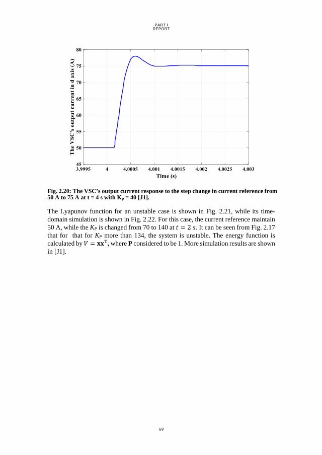
PART I REPORT
69
Fig. 2.20: The VSC’s output current response to the step change in current reference from 50 A to 75 A at t = 4 s with Kp = 40 [J1].
The Lyapunov function for an unstable case is shown in Fig. 2.21, while its time-
domain simulation is shown in Fig. 2.22. For this case, the current reference maintain
50 A, while the KP is changed from 70 to 140 at 𝑡 = 2 𝑠. It can be seen from Fig. 2.17
that for that for KP more than 134, the system is unstable. The energy function is
calculated by 𝑉 = 𝐱𝐱𝐓, where P considered to be 1. More simulation results are shown
in [J1].
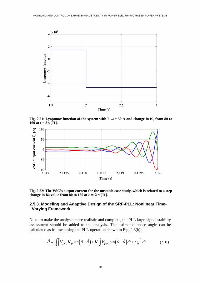
MODELING AND CONTROL OF LARGE-SIGNAL STABILITY IN POWER ELECTRONIC-BASED POWER SYSTEMS
70
Fig. 2.21: Lyapunov function of the system with Id.ref = 50 A and change in Kp from 80 to 160 at t = 2 s [J1].
Fig. 2.22: The VSC’s output current for the unstable case study, which is related to a step change in KP value from 80 to 160 at 𝒕 = 𝟐 𝒔 [J1].
2.5.3. Modeling and Adaptive Design of the SRF-PLL: Nonlinear Time-Varying Framework
Next, to make the analysis more realistic and complete, the PLL large-signal stability
assessment should be added to the analysis. The estimated phase angle can be
calculated as follows using the PLL operation shown in Fig. 2.3(b):
ˆ ˆ ˆsin i s npcc p i pcc nV K K V dt dt (2.31)
Time (s)
VS
C o
utp
ut
curr
ent
𝒊 𝒄 (
A)

PART I REPORT
71
To assess the large-signal stability of the SRF-PLL, a large disturbance in the input
signal is considered. All variables ( ��𝑝𝑐𝑐, ��, ��, and ��) can be considered as the case
studies. However, the SRF-PLL can be normalized to its input’s magnitude, so it will
be insensitive to ��𝑝𝑐𝑐. On the other hand, �� and �� are dependent variables. Hence,
only changes in �� and �� are considered in the case studies. A change in θ is considered
as a phase jump, and change in ω is considered as the frequency deviation.
Considering the phase jump as the input, the model can be rewritten as follows:
ˆ ˆ ˆ ˆcos sin .pcc p pcc iV K V K
(2.32)
By defining 1ˆx and 2
ˆx
, the model can be represented as follows:
1 2
2 2 1 1cos sin .pcc p pcc i
x x
x V K x x V K x
(2.33)
However, if the frequency deviation is considered as a disturbance in the input, the
model can be represented as follows:
ˆ ˆsinn p i pccK K V t t (2.34)
which leads to:
ˆ ˆ ˆcos sinˆ .
ˆ ˆ ˆ1 cos 1 cos 1 cos
pcc p PCC i
pcc p pcc p pcc p
V K t t V K t t
V K t t t V K t t t V K t t t
(2.35)
The large-signal stability assessment of the PLL can be derived based on the
aforementioned models. However, before getting to that point, it is worth to take a
look at the phase portrait of the nonlinear model of the PLL as shown in Fig. 2.23.

MODELING AND CONTROL OF LARGE-SIGNAL STABILITY IN POWER ELECTRONIC-BASED POWER SYSTEMS
72
Fig. 2.23: Phase portrait of a phase jump state trajectory of the nonlinear model of the PLL described in (2.33) for different initial values (Init.) of the phase jump [J2].
As it can be seen from Fig. 2.23, no matter where the initial value for the phase jump
is, the state trajectories will always become stable in infinite time. However, for the
frequency deviation in the input signal, the following limitations should be calculated.
Considering (2.35), if the system becomes stable after the transient, then �� − �� = 0,
which leads to the following equation:
ˆ ˆ ˆcos sinlim 0.
ˆ ˆ ˆ1 cos 1 cos 1 cos
PCC p PCC i
t PCC p PCC p PCC p
V K t t V K t t
V K t t t V K t t t V K t t t
(2.36)
Considering the stable mode for the PLL, the infinite value of t will be much larger
than ω, ��, and their deviation. With this in mind, the second and third terms in (2.36)
are zero. Then, (2.36) can be simplified as follows:
ˆ ˆcos ˆlim lim 0.
ˆ1 cos
PCC p
t tPCC p
V K t t
tV K t t t
(2.37)
If the frequency deviation can be modeled as a first-order function, then the system
will be stable. However, for the order more than one, a nonlinear stability analysis
technique should be used to evaluate the system stability.
To evaluate the global stability of the SRF-PLL control system shown in Fig. 2.3, a
Lyapunov function can be used as follows:
𝜔−
𝜔 (
Hz)
𝜃 − �� (rad)

PART I REPORT
73
21
ˆP2
V (2.38)
Considering (2.35) and (2.38),the Lyapunov function derivative with respect to a time
can be calculated as follows:
ˆ ˆ ˆcos sinˆP
ˆ1 cos
pcc p pcc i
pcc p
V K t t V K t tV
V K t t t
(2.39)
which leads to:
2ˆ ˆ ˆ ˆP cos P sin ˆP
.ˆ ˆ ˆ1 cos 1 cos 1 cos
pcc p pcc i
pcc p pcc p pcc p
V K t V K tV
V K t t t V K t t t V K t t t
(2.40)
For the positive and negative value of , the following inequality can be obtained:
ˆ.
ˆ
pcc p
pcc i
V Kt
V K
(2.41)
By multiplying both sides of the inequality in (2.41) to |𝑉𝑝𝑐𝑐𝐾𝑖(𝜔 − ��)|, it can be
rewritten as follows:
ˆ ˆ .pcc p cp i cK V K t V (2.42)
In this manner, for a conservative case, to satisfy the Lyapunov stability constraints,
the following inequality should be satisfied:
ˆ .pcp cK V (2.43)
This means that if the inequality in (2.43) is satisfied, the system will remain stable.
In this manner, a modified SRF-PLL is proposed in [J2], which is also shown in Fig.
2.24, where 𝜆𝑓𝑐 is an adaptive gain (which is a real positive number). �� and �� are the
estimated frequency and the estimated initial phase of the input signal. 𝜆𝑓𝑐 acts as a
gain that damps the transient fluctuation of the estimated frequency, as it is later
shown and discussed in Fig. 2.28 and Fig. 2.29.
By applying the proposed adaptive SRF-PLL, the following inequality is satisfied,
which leads to global stability:
ˆ
1 .p pccK V
(2.44)
More results are presented in [J2]. It is worth mentioning that the adaptive gain shown
in Fig. 2.24 will become smaller and smaller as the estimated phase angle gets closer

MODELING AND CONTROL OF LARGE-SIGNAL STABILITY IN POWER ELECTRONIC-BASED POWER SYSTEMS
74
to its actual value. This means that the proposed adaptive SRF-PLL will act as a
common SRF-PLL in the steady-state mode of the system.
Fig. 2.24: Block diagram of the proposed adaptive SRF-PLL [J2].
The estimated frequency by the SRF-PLL, shown in Fig. 2.3, with different phase
jumps are shown in Fig. 2.25.
Fig. 2.25: Time domain simulations of the SRF-PLL subjected to different phase jumps for system shown in Fig. 2.3 [J2].
Experimental tests for the same scenarios are shown in Fig. 2.26 and Fig. 2.27.
iK
ˆˆt
sin
cos
dq
abc
abcVn
ˆ
1ˆ
PCC
fc
V
pK
qV q
pcc
V
V
v
v
K
s K
dVPCCV
fc
ˆ
Time (s)
Est
imat
ed f
requ
ency
(H
z)

PART I REPORT
75
Fig. 2.26: The SRF-PLL estimated frequency for different phase-jumps (experimental results). π/6 phase jump implement to the PLL and it is cleared after 200 ms [J2].
Fig. 2.27: The SRF-PLL estimated frequency for different phase-jumps (experimental results). 5π/6 phase jump implement to the PLL and it is cleared after 200 ms [J2].
By using the adaptive SRF-PLL, the performance of the system improved as shown
in Fig. 2.28 and Fig. 2.29. Its experimental verification are presented in [J2]. In Fig.
2.28, the frequency is estimated by the standard SRF-PLL as shown in Fig. 2.3 (green
dashed line), and also it is estimated by the adaptive SRF-PLL shown in Fig. 2.24 with
Est
imat
ed f
req
uen
cy (
Hz)
30
45
35
40
50
60
65
70
55
40 ms
Est
imat
ed f
req
uen
cy (
Hz)
30
45
35
40
50
60
65
70
55
40 ms

MODELING AND CONTROL OF LARGE-SIGNAL STABILITY IN POWER ELECTRONIC-BASED POWER SYSTEMS
76
two different adaptive gain values. For this case study, the input frequency is changed
from 50 Hz to 48.5 Hz within 0.01 s. In Fig. 2.29, the same conventional SRF-PLL
and the adaptive SRF-PLL is tested for 30⁰ phase jump in the input. As it can be seen
from Fig. 2.28 and Fig. 2.29, the input frequency estimation is improved by using the
adaptive SRF-PLL in comparison with the conventional one. Values for 𝜆𝑓𝑐 are
chosen randomly, however, this can be tuned for a specific case study.
Fig. 2.28: Estimated frequency by the SRF-PLL for second-order input frequency deviation from t = 1 s to t = 1.01 s using the proposed adaptive tuning method with different damping factors [J2].
Fig. 2.29: Estimated frequency by the SRF-PLL for 30⁰ phase jump at t = 1 s using the proposed adaptive tuning method with different damping factors [J2].
2.6. Summary
Grid-feeding power converters are becoming more popular in power systems, and this
chapter study the large-signal stability of the grid-tied VSCs. It starts with highlighting
the importance of grid-feeding power converters stability assessment. Then, align
Time (s)
Est
imat
ed f
req
uen
cy (
Hz)
E
stim
ated
fre
qu
ency
(H
z)
Time (s)

PART I REPORT
77
with the main focus of this Ph.D. project, a large-signal model of the grid-tied VSC
using the Lyapunov stability theory is presented. Furthermore, the SRF-PLL nonlinear
model stability is analyzed by using the portrait phase concept and the Lyapunov
theory. In addition, two nonlinear stability assessment techniques are discussed, as
they are used for large-signal stability analysis of the nonlinear models.
Related Publications
J1. B. Shakerighadi, E. Ebrahimzadeh, F. Blaabjerg, and C. L. Bak, ‘‘Large-
signal stability modeling for the grid-connected VSC based on the Lyapunov
method,’’ in Energies, vol. 11, p. 2533, Oct. 2018.
Main contribution:
In this paper, the large-signal model of the grid-tied VSC based on its
Lyapunov function is proposed. The time delay caused by the PWM
switching is also considered in the model. A systematic approach is
developed to find the parametric Lyapunov function of the grid-tied VSC.
J2. B. Shakerighadi, E. Ebrahimzadeh, M. G. Taul, F. Blaabjerg and C. L. Bak,
"Modeling and Adaptive Design of the SRF-PLL: Nonlinear Time-Varying
Framework," in IEEE Access, vol. 8, pp. 28635-28645, 2020.
Main contribution:
In this paper, a non-linear time varying (NTV) model of the PLL is developed
in order to assess the large-signal stability of it. Both the phase portrait method
and the Lyapunov function are used to analyze the PLL large-signal stability.
An adaptive model of the SRF-PLL is proposed to improve its performance
for large disturbances.
C1. B. Shakerighadi, E. Ebrahimzadeh, F. Blaabjerg and C. L. Bak, "Lyapunov-
and Eigenvalue-based Stability Assessment of the Grid-connected Voltage
Source Converter," 2018 IEEE International Power Electronics and
Application Conference and Exposition (PEAC), Shenzhen, 2018, pp. 1-6.
Main contribution:
The stability of the grid-tied VSC is assessed by using two methods: A small-
signal stability and the large-signal stability. It is shown that for a grid-tied
VSC, how the second order Lyapunov function should be defined. It is shown
that in analyzing a linear system, the large-signal stability assessment leads
to the same result as small-signal methods.
C2. B. Shakerighadi, E. Ebrahimzadeh, C. L. Bak and F. Blaabjerg, " Large
Signal Stability Assessment of the Voltage Source Converter Connected to a
Weak Grid," Proceedings of Cigre Symposium Aalborg 2019, 2019, pp. 1-
12.
Main contribution:

MODELING AND CONTROL OF LARGE-SIGNAL STABILITY IN POWER ELECTRONIC-BASED POWER SYSTEMS
78
In this paper, the impact of the weak grid on the large-signal stability of the
system is modeled and is assessed.

PART I REPORT
79
Chapter 3.
Large-Signal stability of Power-
electronic-based power systems
3.1. Abstract
In this Chapter, relevant topics regarding the security and the large-signal stability of
large-scale the PE-based power systems are presented. The chapter starts with
proposing a guideline for security assessment of modern power systems. Then, a
discussion regarding the inertial response of a single grid-tied VSC is presented.
Finally, a proposed method for the large-signal stability assessment of PE-based
power systems is presented, where a method to aggregate inertia is presented.
3.2. Background and motivation
PE-based units play an important role in modern power systems stability, security,
and reliability assessments [6], [53]. Increasing the penetration of PE-based energy
sources, such as wind turbines and photovoltaics, introduces new challenges in
stability and security of power system [76]. It is interesting to know how the maximum
penetration of PE-based energy sources should be determined for a power system in
order to make sure that system remains stable for a credible contingency [42]. Talking
about a credible contingency, the assessment of large disturbances in PE-based power
systems needs a more careful consideration and analysis to have a better
understanding of the grid stability. The main goal of this chapter is to analyze how a
large disturbance can affect a PE-based power system stability. A key point is the
system inertial response, due to the increase the PE-based unit’s penetration, the
system equivalent inertia will decrease as it is discussed later.
3.3. Security Assessment of PE-based Power Systems
As the scale of the power systems increases from a grid-tied VSC to a large-scale
power system, the large-signal stability assessment needs to use a different approach.
In respect to the single grid-tied VSC, a detailed control system model can be used to
assess the stability; however, in large-scale power systems, the grid behavior is more
important than the detailed model of the system. The reason is that using the detailed
model of the large-scale power system is impractical, while, it might be of importance

MODELING AND CONTROL OF LARGE-SIGNAL STABILITY IN POWER ELECTRONIC-BASED POWER SYSTEMS
80
for the system stability analysis. Besides, most often, the detailed model of the power
systems, including all component details, is not available1.
As mentioned previously, the stability challenges of modern power systems2 may lead
to blackouts [28], [103], which is not only important from the stability point of view,
but it is also a great deal for the system security. An overall schematic of the security
assessment of power systems with a high penetration of PE-based units is shown in
Fig. 3.1.
The power systems security is defined as its ability to maintain its stability when it is
subjected to a contingency [27]. Based on that, the modern power system security
analysis can be categorized as shown in Fig. 3.2, where it is divided into three
categories: static security, dynamic and transient security, and cyber security. In static
security, static constraints of the system in its normal condition and when it is
subjected to a contingency are checked. Regarding the dynamic and transient security,
system oscillatory modes and transient stability during the normal and contingency
conditions are checked. The cyber security assessment of modern power systems is
related to its ability to remain stable when it is subjected to a cyber-attack like false
data injection [97]. The first two security subcategories are studied here, and the
cyber-security assessment is trended as out of the scope of this project but becomes
more and more important.
1 Most often, renewable energy-related companies, such as wind turbine manufacturers, are not
willing to share their product models with system operators (or anyone out of their companies),
due to the market competition and technology. In this circumstance, although specific grid
codes are required from wind turbine manufacturers, the system operators do not have the full
model of the system, and they are analyzing the grid stability based on their knowledge of the
system model that they have. Therefore, this makes the system operators to rely on the system
variables that could be measured, like the bus voltages and the system frequency, rather than
the detailed system models.
2 Stability challenges of the power system are categorized into three main subcategories: rotor
angle stability, frequency stability, and voltage stability.

PART I REPORT
81
Fig. 3.1: Overall schematic of the security assessment of power systems with a high penetration of PE-based units [J3].
Fig. 3.2: Power system security assessment categories including both static and dynamic analysis [J3].
A guideline for the security assessment of the PE-based power systems is proposed
and it is shown in Fig. 3.3 and Fig. 3.4. In this guideline, the importance of PE-based
Power-Electronic-
based (PE-based)
Power System
Security Assessment
Transient
security
Dynamic
securitySteady-
state
security
Power System Security
Power Electronic System Security
Transient
security
Dynamic
securitySteady-
state
security
System level
Security
alert
Failure
modes
Condition
monitoring
Component level
Security
StaticDynamic &
Transient
Cyber
Security
EMM
Stability
Frequency
Stability
Angular
Stability
Voltage
Stability
Voltage
Stability
Thermal
Stability
MODELING AND CONTROL OF LARGE-SIGNAL STABILITY IN POWER ELECTRONIC-BASED POWER SYSTEMS
82
units on the system security is highlighted. The security assessment of PE-based
power systems may be done in three steps: static security assessment, dynamic
security assessment, and the transient security assessment. In the static security
assessment, just like the security assessment of the conventional systems, the load
flow of the system in its normal condition as well as N-1 contingency situation is
derived to check the static security constrains. The static security constrains, for
instance, include the line thermal constrains and their maximum transferrable active
power. If the system passes all the static security checks, then the dynamic security
constrains of the system should be checked. In this phase, first a small-signal model
of the system in the normal operation and N-1 contingency conditions are used to
further check the oscillatory modes of the system. If all oscillatory modes of the
system are damped both locally and globally, then the system is dynamically secure.
Next, the transient security of the system should be checked. At this stage, the
transient stability of the system is subjected to a large (and small) disturbances and
should be analyzed, and if the system provides sufficient response that meets the grid
codes, then the system is called transient secure. This process is shown in Fig. 3.3 and
Fig. 3.4, respectively.

PART I REPORT
83
Fig. 3.3: PE-based power system security assessment: Static security assessment [J3].
Are all electric and
thermal constraints
within their limits?
i=1
Yes
No
ith equipment is
out of order
Load Flow
(N-1)
Are all electric and
thermal constrains within
their limits?
System security is
not guaranteed
Yes
i=i+1
No
System Security is not
guaranteed
Load Flow
(N)
System static Security is
guaranteed
Apply remedial
action
Apply remedial
action
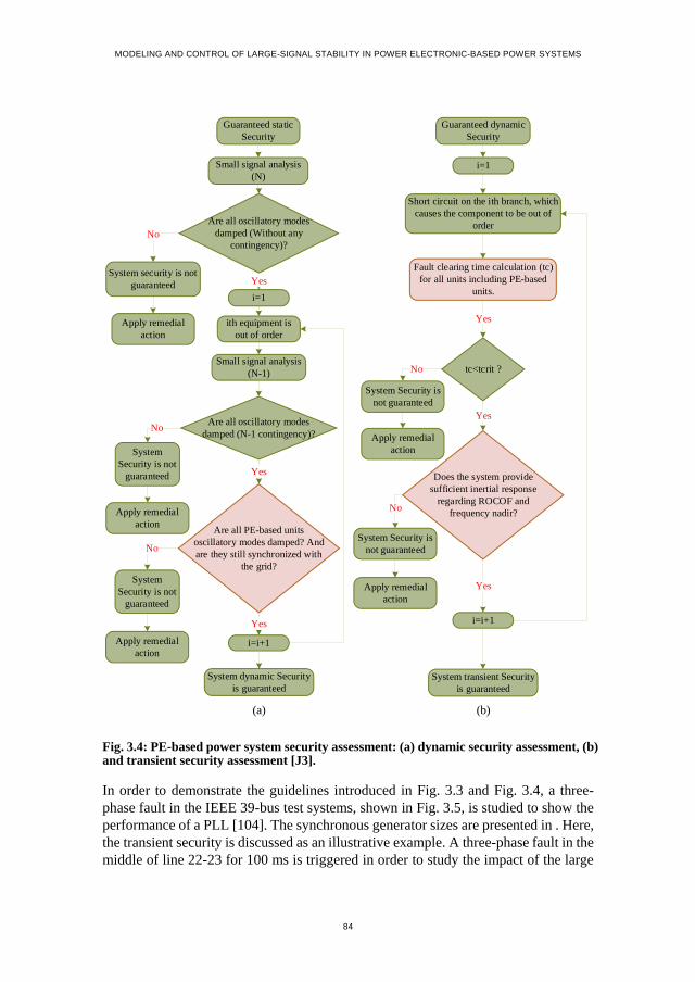
MODELING AND CONTROL OF LARGE-SIGNAL STABILITY IN POWER ELECTRONIC-BASED POWER SYSTEMS
84
Fig. 3.4: PE-based power system security assessment: (a) dynamic security assessment, (b) and transient security assessment [J3].
In order to demonstrate the guidelines introduced in Fig. 3.3 and Fig. 3.4, a three-
phase fault in the IEEE 39-bus test systems, shown in Fig. 3.5, is studied to show the
performance of a PLL [104]. The synchronous generator sizes are presented in . Here,
the transient security is discussed as an illustrative example. A three-phase fault in the
middle of line 22-23 for 100 ms is triggered in order to study the impact of the large
Are all oscillatory modes
damped (Without any
contingency)?
i=1
Yes
No
ith equipment is
out of order
Small signal analysis
(N-1)
Are all oscillatory modes
damped (N-1 contingency)?
System security is not
guaranteed
i=i+1
No
System
Security is not
guaranteed
Guaranteed static
Security
System dynamic Security
is guaranteed
Small signal analysis
(N)i=1
Short circuit on the ith branch, which
causes the component to be out of
order
Fault clearing time calculation (tc)
for all units including PE-based
units.
tc<tcrit ?
i=i+1
Guaranteed dynamic
Security
System transient Security
is guaranteed
Yes
No
System Security is
not guaranteed
Yes
(a) (b)
Yes
Are all PE-based units
oscillatory modes damped? And
are they still synchronized with
the grid?
System
Security is not
guaranteed
No
Yes
Does the system provide
sufficient inertial response
regarding ROCOF and
frequency nadir?
Yes
System Security is
not guaranteed
No
Apply remedial
action
Apply remedial
action
Apply remedial
action
Apply remedial
action
Apply remedial
action

PART I REPORT
85
disturbance on the grid-tied VSC. In this scenario, it is assumed that instead of the
generator connected at bus 22, a wind turbine with the same power rating is
substituted. The wind turbine is modeled as a grid-feeding power converter as
discussed in 2.5. The voltage magnitude and phase angle at bus 22 are shown in Fig.
3.6. As it can be seen from Fig. 3.6(b), a three-phase short circuit fault causes a 20⁰
phase angle change at bus 22. The PLL response for the aforementioned fault at line
22-23 is shown in Fig. 3.7, where a 20⁰ phase angle deviation leads to a more than 3
Hz frequency estimation error. If the protection system of the PE-based unit is
sensitive to this frequency deviation, the unit may be disconnected from the system as
a result of a false frequency estimation [67]. As it is mentioned before, this simulation
is presented as an illustrative example. More details are discussed later in Scenario 1-
3.
Table 3.1: IEEE 39-bus test system generator sizes.
Generator Type
Size
Rating power
[MVA]
Active power
[MW]
Voltage magnitude
at the output
terminal [p.u.]
G1 PV 10000 1000 1.03
G2 Slack 630 0 0.982
G3 PV 720 585 0.9831
G4 PV 720 568 0.9972
G5 PV 270 229 1.0123
G6 PV 720 585 1.0493
G7 PV 630 504 1.0635
G8 PV 900 747 1.0278
G9 PV 1000 830 1.0265
G10 PV 1000 250 1.0475

MODELING AND CONTROL OF LARGE-SIGNAL STABILITY IN POWER ELECTRONIC-BASED POWER SYSTEMS
86
Fig. 3.5: IEEE 39-bus test system used for security assessment, where a three-phase short circuit is indicated in the middle of line 22-23 [104].
G8
G10
G1
G2
G3
G5 G4
G7
G6
G91
2
3
4
5
6
7
8
9
10
11
12
13
14
15
16
17
18
19
20
2122
23
24
25 26
27
28 2930
31
32
3334
35
36
38
38
39
A Three-phase fault

PART I REPORT
87
Fig. 3.6: Bus 22 (a) voltage phase angle, (b) and its voltage magnitude, for a three-phase fault happening at t = 100 ms, and cleared at t = 200 ms [C3].
Fig. 3.7: Frequency estimation of the PLL for 20⁰-phase-jump at t = 100 ms caused by a near three-phase fault, which is cleared at t = 200 ms [C3].
Three scenarios are discussed in this system to show the impact of increasing the PE-
based units’ penetration in power systems. The first scenario explains the
conventional stability issues, while in the next two scenarios the grid stability with
different NSG penetration levels is discussed. Case studies are derived on the same
IEEE 39-bus test system and developed in DigSILENT PowerFactory, like shown in
2. 001. 601. 200. 800. 400. 00 [ s]
1. 25
1. 00
0. 75
0. 50
0. 25
0. 00
[ p. u. ]
Bus 23: Volt age, Magnit ude
2. 001. 601. 200. 800. 400. 00 [ s]
30. 00
20. 00
10. 00
0. 00
- 10. 00
- 20. 00
[ deg]
Bus 23: Volt age, Angle
DIgSILENT 39 Bus New England Syst em SubPlot
Simulat ion Fault Bus 16 St able
Dat e: 5/ 2/ 2019
Annex: / 5
1.25
1.00
0.75
0.50
0.25
0.00 0.40 0.80 1.20 1.60 2.00
30.00
20.00
10.00
0.00
-10.00
Vo
lta
ge A
ng
le [
deg
]V
olt
ag
e M
ag
nit
ud
e [
p.u
.]
0.00 0.40 0.80 1.20 1.60 2.00Time [s]
0.00
-20.00
(a)
(b)

MODELING AND CONTROL OF LARGE-SIGNAL STABILITY IN POWER ELECTRONIC-BASED POWER SYSTEMS
88
Fig. 3.5. For these scenarios, the NSG is considered as a fully controlled wind turbine
that has a current controller, active and reactive power controller, active power
reduction for the over-frequency, and two PLLs as shown in Fig. 3.8. One PLL is used
for estimating system phase angle that is used for the current controller and the other
one (that is slower than the first PLL) is used for measuring the frequency for over-
frequency active power reduction. It should be mentioned that the over-frequency
active power reduction will not be activated in Scenario 1 to 3 due to low over
frequency. Accordingly, the wind turbine controller can be simplified as a current
controller and active and reactive power controllers, which represents a grid-feeding
power converter discussed in Chapter 2. The wind turbine controller parameters used
here for the simulation are given in Table 3.2. There are also more specific details
regarding the wind turbine controller that is used here, which is presented in [105]. It
is also should be mentioned that the size of the wind turbine is considered as if it
replaced with a synchronous generator, it produce the same rating power. To do so,
for instance, to replace a 600 MVA synchronous generator, 240 wind turbines with
2.5 MVA rating power that are connected in parallel, are used. In this way, the same
steady-state behavior will be presented by changing the NSG penetration, however, a
different dynamic response is introduced.
Fig. 3.8: Wind turbine control block diagram used in the IEEE 39-bus test system for the security assessment of the grids with different level of NSG penetration.

PART I REPORT
89
Table 3.2: Wind turbine current controller and active and reactive power controllers parameters.
Controller
parameter
value Description
Kq 1 Gain reactive current controller [-]
Tq 0.002 Integrator time constant reactive current controller [s]
Kd 1 Gain active current controller [-]
Td 0.002 Integrator time constant active current controller [s]
Kp 0.5 Active power control gain [p.u.]
Tp 0.002 Active power control time constant [s]
Kq 0.5 Reactive power control gain [p.u.]
Tq 0.02 Reactive power control time constant [s]
imax 1 Current magnitude limit [p.u.]
Scenario 1: Conventional power system
In this scenario, it is assumed that all generators are based on conventional energy
sources (synchronous generators). G2 is considered as the reference synchronous
machine. A generation trip is studied for all case studies. Here, G5 is tripped at t = 50
s and it is considered as the large disturbance. The voltage magnitude at Bus 6, 25,
and 28 as well as the system frequency are shown in Fig. 3.9 and Fig. 3.10,
respectively. Fig. 3.10 presents the frequency response of the system, where the
synchronous generators’ governor response is shown in Fig. 3.10(a). It is worth
mentioning that the governor response is slower than the inertial response of the
synchronous generator [106].

MODELING AND CONTROL OF LARGE-SIGNAL STABILITY IN POWER ELECTRONIC-BASED POWER SYSTEMS
90
Fig. 3.9: Bus 6, 25, and 28 voltage magnitude response to G5 trip at t = 50 s for the conventional power system case study (Scenario 1) [J3].
Fig. 3.10: System frequency response to the G5 trip at t = 50 s (a) including the governor response, and (b) zoom in figure with the same time scale of Fig. 3.9 (Scenario 1) [J3].
As it can be seen from Fig. 3.10, the loss of generation causes imbalance between the
load and generation that leads to drop in frequency. This means that rotor speed in the
other generators drop right after the fault occur with respect to each generator’s inertia.
However, this event converge to a new stable operating point. This large disturbance
causes a fluctuation in voltage magnitude of grid nodes as shown in Fig. 3.9.
(a)
(b)

PART I REPORT
91
Scenario 2: PE-based power systems with a penetration level of 11.2%
In this scenario, instead of G4, a wind farm with the same power rating is substituted.
The NSG penetration is 11.2% for this case study. The NSG used here is the wind
turbine, which model is presented in Fig. 2.1, and also discussed in [105], where active
and reactive current controller proportional gains are 1 and its integrator time
constants for active and reactive powers are 0.002. The voltage magnitudes at Bus 6,
25, and 28 and system frequency are shown in Fig. 3.11 and Fig. 3.12 for the same
event of that discussed in Scenario 1, respectively.

MODELING AND CONTROL OF LARGE-SIGNAL STABILITY IN POWER ELECTRONIC-BASED POWER SYSTEMS
92
Fig. 3.11: Bus 6, 25, and 28 voltage magnitude response to generator 5 trip at t = 50 s for the PE-based power system case study (Scenario 2) [J3].
Fig. 3.12: The PE-based power system frequency response to the generator 5 trip at t = 50 s for the PE-based power system Case study (a) including the governor response, and (b) zoom in figure with the same time scale of Fig. 3.11 (Scenario 2) [J3].
The equivalent inertia of the grid with 11.2% wind turbine penetration is less than the
grid with 100% synchronous generators. A proposed method to determine the
equivalent grid inertia is discussed later in this chapter; however, It can be seen that a
system with a higher penetration of RES has a lower inertial response. This can be
seen by comparing Fig. 3.10 and Fig. 3.12, as the frequency nadir is lower in the case
(a)
(b)

PART I REPORT
93
with a higher wind turbine penetration. The relatively low frequency nadir in Fig. 3.12
leads to a higher voltage magnitude fluctuation shown in Fig. 3.11, in comparison
with the voltage magnitude fluctuation shown in Fig. 3.9. The grid is still stable in
this case study, while it faces more voltage and frequency fluctuations in comparison
with the case study discussed in Scenario 1.
Scenario 3: PE-based power systems with high penetration of wind power
(43.6% penetration level)
In this scenario, G3, G4, G6, G7, and G8 are substituted with wind farms with the
same power rating. The NSG penetration is 43.6% for this case study. The voltage
magnitude at Bus 6, 25, and 28 and system frequencies are shown in Fig. 3.13 and
Fig. 3.14, respectively.
Fig. 3.13: Bus 6, 25, and 28 voltage magnitude response to G5 trip at t = 50 s for the system with high penetration of wind turbine (43.6%) (Scenario 3).
Fig. 3.14: The PE-based power system frequency response to the G5 trip at t = 50 s for the system with high penetration of wind turbine (43.6%) (Scenario 3) [J3].
As it can be seen from Fig. 3.13 and Fig. 3.14, the grid becomes unstable in this case
study. The wind turbine penetration is relatively high (43.6%); however, the wind
turbine penetration is not distributed in the grid at the same rate in all generation
points. With the same penetration level of wind turbines in the grid for all generation

MODELING AND CONTROL OF LARGE-SIGNAL STABILITY IN POWER ELECTRONIC-BASED POWER SYSTEMS
94
points (G1-10), a higher penetration of wind turbine can be achieved without
becoming unstable, as discussed in the next part.
Although the abovementioned analysis indicates stability challenges introduced by
the increase of PE-based unit’s penetration in power system, a mathematical model
that describes the transient stability of such a system is needed, which is proposed in
Section 3.5.
3.4. Semi-inertial response of the grid-feeding power converters
Although it has been mentioned in the literature that the grid-feeding power converter
does not provide any inertial response, in this section the large-signal stability of the
grid-tied VSC is assessed based on its semi-inertial response [7], [C4]. It should be
mentioned that this chapter is dedicated to the large-signal stability of large-scale
power systems, while the inertial response of a single grid-tied VSC is assessed in this
section. The analysis of inertial response of a single grid-tied VSC is prerequisite for
the inertial response of large-scale PE-based power systems, as it is studied in the next
section.
Considering the grid-feeding power converter as it is shown in Fig. 2.4 and Fig. 2.5,
the output active power and current can be given as follows:
3 cos
sin
e G d
Gd
L
P V I
VI
X
(3.1)
where Id is the output current of the VSC in the d-axis. Considering the
aforementioned equations, the output power can be calculated as follows:
2
1.5 sin 2 .Ge
L
VP
X (3.2)
Based on the current control loop, the VSC current can be determined as follows:
2
* 1.5 sin 2 .Gd P i
L
VI K K P
X
(3.3)
Based on that, the derivative of the phase angle can be determined as follows:
2*
2
1.5 sin 2
.cos 3 cos 2
Gi L
L
G P G
VK X P
X
V K V
(3.4)

PART I REPORT
95
Considering the following calculation for the second order derivative of the phase
angle as:
2
2,
d d d d d d d
dt dt dt d dt ddt
(3.5)
it can be calculated as follows:
222 *
2
22
32
22 *
32
1.5 sin 2
3 cos 2 cos 3 cos 2
cos 3 cos 2
sin 6 sin 2 1.5 sin 2
.
cos 3 cos 2
Gi L
L
GG P G
L
G P G
GG P G
L
G P G
VdK X P
Xdt
VV K V
X
V K V
VV K V P
X
V K V
(3.6)
By defining the following index based on the similar behavior of the synchronous
generator’s swing equation, called semi-moment of inertia (SMOI), the system
stability can be diagnosed:
*
2
2
, , .e
G
P PSMoI V t
d
dt
(3.7)
For positive values of SMoI, the system is stable, while if the index becomes negative,
the system is unstable. The stability margin is reached when SMoI equals zero.
Considering the grid-feeding model presented in Fig. 2.4 and Fig. 2.5 with the
configuration presented in Table 3.3, three case studies are done to assess the proposed
mathematical model.
Table 3.3: System parameters of a grid-tied VSC [C4].
System parameter Value Explanation
Lf-filter 10 mH An L-filter is considered at the output of the
VSC to smooth the system output current.
Lg 0 mH-10 mH-
100 mH
The 0 mH introduces the stiff grid, while 10 mH
and 100 mH are used for the weak grid and very
weak grid conditions, respectively.

MODELING AND CONTROL OF LARGE-SIGNAL STABILITY IN POWER ELECTRONIC-BASED POWER SYSTEMS
96
Considering 𝑆𝑏𝑎𝑠𝑒 = 15 𝑘𝑉𝐴 and 𝑉𝑏𝑎𝑠𝑒 =
400 𝑉, the SCR for 0 mH, 10 mH, and 100 mH
equal infinite, 4 p.u., and 0.4 p.u., respectively.
Vg 400 V (rms
phase to phase)
An ideal three-phase voltage source is used for
assessing the inertial response.
System frequency 50 Hz
Ts 10-4 s The sampling frequency is 10 kHz.
Smax 15 kVA Maximum apparent power (power level)
Case study 1: Impact of increasing the VSC output power on the system stability and
its relation to the SMoI index
In this case study, the output power reference is changed from 4 kW to 14 kW, as
shown in Fig. 3.15. As it can be seen from Fig. 3.16, the output power follows its
reference. However, as the output power gets closer to the maximum transferrable
active power, the SMoI index decreases, which means that the operating point is
getting closer to its stability margin3.
3 The definition of the maximum transferrable active power is discussed in Section 2.5.1,
specifically in (2.22). The same concept is used here as well.

PART I REPORT
97
Fig. 3.15: Maximum transferable (𝑷𝒎𝒂𝒙), reference (𝑷𝒓𝒆𝒇), and output active power (𝑷𝒆)
of the grid-connected VSC with a step change in the active power reference at t = 2 s from 4 kW to 14 kW [C4].
Fig. 3.16: The Semi-Moment of Inertia (SMoI) of the grid-connected VSC with a step change in active power reference at t = 2 s from 4 kW to 14 kW [C4].
Case study 2: Impact of the weak grid on the system stability and its relation to the
SMoI index

MODELING AND CONTROL OF LARGE-SIGNAL STABILITY IN POWER ELECTRONIC-BASED POWER SYSTEMS
98
Here, the impact of the grid impedance on the system stability and its relation with
the SMoI index is studied. To do so, the grid impedance is doubled at 𝑡 = 2 𝑠, which
leads to a decrease in maximum transferrable active power, as shown in Fig. 3.17.
Like in Case study 1, the SMoI decreases as the operating point gets closer to the
stability boundary, as shown in Fig. 3.18.
Fig. 3.17: Maximum transferable (𝑷𝒎𝒂𝒙), reference (𝑷𝒓𝒆𝒇), and output active power (𝑷𝒆)
of the grid-connected VSC with a step change in 𝒁𝒈 (making 𝒁𝒈 twice of its initial value)
at t = 2 s and 3 s [C4].

PART I REPORT
99
Fig. 3.18: The Semi-Moment of Inertia (SMoI) index of the grid-connected VSC with a step change in 𝒁𝒈 (making 𝒁𝒈 twice of its initial value) at t = 2 s and 3 s [C4].
Case study 3: analyzing the stability marginal point by using the SMoI index
The marginal point of stability is when the SMoI index becomes zero. In this
circumstance, the system introduces a negative semi-inertial response, which is
physically unstable condition. To demonstrate this scenario, grid impedance is
changes into a large value (eight times of the base value). Then, when the active power
reference is larger than the maximum transferrable power, the system will become
unstable. The active power reference, the output active power, and the maximum
active power are shown in Fig. 3.19. The SMoI index is also shown in Fig. 3.20, where
it can be seen that the index becomes negative for the period that the system works in
its unstable mode.

MODELING AND CONTROL OF LARGE-SIGNAL STABILITY IN POWER ELECTRONIC-BASED POWER SYSTEMS
100
Fig. 3.19: Maximum transferable (𝑷𝒎𝒂𝒙), reference (𝑷𝒓𝒆𝒇), and output active power (𝑷𝒆)
of the grid-connected VSC with a large step change (eight times) in 𝒁𝒈 at t = 2 s and 3 s
[C4].
Fig. 3.20: The Semi-Moment of Inertia (SMoI) index of the grid-connected VSC with a with a large step change (eight times) in 𝒁𝒈 at t = 2 s and 3 s [C4].

PART I REPORT
101
It should be mentioned that the mathematical model is presented in Fig. 3.19 and Fig.
3.20. The time-domain simulation results of this scenario derived in Matlab/Simulink
is presented in Fig. 3.21, where the instability can be seen from the VSC three-phase
current.
Fig. 3.21: Time-domain simulation for the unstable case study (Case study 3). (a)VSC
three-phase output current and (b) the PCC three-phase voltage.
In conclusion of this part, it is shown that the grid-feeding power converter introduce
a semi-inertial response to the system fluctuations, which can be determined by SMoI
index. This inertial response is provided by the lag between the reference and actual
active power of the VSC, due to the integral gain included in the active power control
loop.
3.5. Transient stability of power-electronic-based power systems
In order to do transient stability analysis of large-scale PE-based power systems, the
Lyapunov function theory and the equal area criterion can be used [59]. In this way,
the same concept developed for the grid-tied synchronous generator can be extended
to analyze the large-scale PE-based power system stability. Considering a grid-tied
synchronous generator as shown in Fig. 3.22.
(a)
(b)

MODELING AND CONTROL OF LARGE-SIGNAL STABILITY IN POWER ELECTRONIC-BASED POWER SYSTEMS
102
Fig. 3.22: A single-line diagram of the synchronous machine with impedance 𝑿𝒔 connected to the grid through a line with impedance 𝑿𝒈.
The active power transferred to the grid is given as:
sins g
e sg s
V VP
X X
(3.8)
where 𝑃𝑒 is the transferred active power. Based on that, the swing equation can be
derived as follows:
m
m e m
dP P J
dt
(3.9)
where 𝑃𝑚 is the mechanical power. 𝜔𝑚 and J are the rotational speed and moment of
inertia, respectively. By using the concept of equal area criterion, the transient
stability of the grid-tied synchronous machine can be explained [22]. The inertia
constant H [s] is furthermore defined as:
20
2
mr
B B
JEH
S S
(3.10)
Here, Er is the rotational energy in the machine [J], ωm0 is the nominal rotational speed
of the machine [rad/s], and SB is the [MVA] rating of the machine. Based on (3.8),
(3.9), and (3.10), the voltage angle between 𝑉𝑠 and 𝑉𝑔 can be determined as follows:
2
0
2 2
e m es
B
P Pd
S Hdt
(3.11)
where 𝜔𝑒0 is the steady state value of the SG’s voltage angle velocity. In this way, by
integrating (3.11) twice, 𝛿𝑠 can be determined at the critical clearing time4 as follows:
2
00
4cr
e m es t t
B
P P tt
S H
(3.12)
4 The critical clearing time is the largest duration for the fault that the system remain stable after
clearing the fault [110].
sX gX 0gVs sV ePmP
m gSynchronous Machine
Rotational speed of Rotor:Infinite Bus
Angular velocity of the grid:

PART I REPORT
103
where 𝛿0 is the synchronous generator’s voltage angle before the fault. Based on
(3.12), the critical clearing time can be calculated as follows:
0
0
4.
B crcr
e m e
S Ht
P P
(3.13)
For the aggregation of multiple synchronous machines, the model can be developed
as follows:
2 2 21 2
1 2
...
2 ...
m m mN rAA
B B BN BA
J J J EH
S S S S
(3.14)
In transient stability analysis, the marginal stability is determined by the critical
clearing time of the fault. The critical clearing time can be determined as follows:
0
0
4 B A crcr
e m e
S Ht
P P
(3.15)
where 2
00
4
e m ecr
B
P P t
S H
. To expand the theory to two grid areas A and B
connected via a long transmission line, the following equation can be assumed for
each of them:
2
0 0
2 2 2
e mA eA e mA eAeA
A A A
P P P Pd
S H Edt
(3.16)
2
0 0
2 2 2
e mB eB e mB eBeB
B B B
P P P Pd
S H Edt
(3.17)
where EA and EB are the total rotational energy for each area. Considering the voltage
phase angle difference between two areas as δeAB= δeA-δeB, the following equation can
be derived:
200 0
2.
2 2 2
e B mA eA A mB eBe mA eA e mB eBeAB
A B A B
E P P E P PP P P Pd
E E E Edt
(3.18)

MODELING AND CONTROL OF LARGE-SIGNAL STABILITY IN POWER ELECTRONIC-BASED POWER SYSTEMS
104
In steady-state, PmA0=PeA0=-PmB0=-PeB0. During a fault due to the interruption in a
transmission line, a surplus of power is created in area A and a deficit of power in area
B. PeA =PmA0 - ΔP, PeB =PmB0 + ΔP. Then,
2
0 0
2.
2 2
e B A e B AeAB
A B A B
E P E P P E Ed
E E E Edt
(3.19)
Defining,
/A B base
eqB A
E E SH
E E
(3.20)
yields
20
2.
2
eAB e
eq base
d P
H Sdt
(3.21)
Integrating twice up to the critical clearing angle as discussed in (3.12):
2
00.
4cr
e cr
t tbase eq
Ptt
S H
(3.22)
Based on (3.22), the critical clearing time for the two-area system can thus be derived
as
0
0
4.
base eq cccr
e
S Ht
P
(3.23)
Note that Sbase can be chosen with an arbitrary value. A conclusion from (3.23) is the
relationship between the critical clearing time and the system inertia constant is given
as follows:
.cr eqt k H (3.24)
Another simpler form of this equation is
0
0
4 eq cccr
e
Et
P
(3.25)
in which the equivalent rotational energy is defined as:
.A Beq
B A
E EE
E E
(3.26)
An important conclusion from (3.20) and (3.26) is that if the inertia in one of the areas
is low, then the equivalent inertia will be low consequently. This means that if 𝐸𝐴 is

PART I REPORT
105
much larger than 𝐸𝐵, then 𝐸𝑒𝑞 = 𝐸𝐵. In practice, if the NSG penetration is not
distributed normally in the system, then a region with a high penetration of NSG
determines the whole system inertial response.
3.5.1. Simulation results
In this part, two case studies on the Kundur two-area test system [59] and the Nordic
23-machine test system [107] are presented to verify the theory discussed in Section
3.5.
3.5.1.1 Testbed 1: Kundur two-area test system
The Kundur two-area test system is shown in Fig. 3.23 [59]. Some basic information
regarding this test system can be found in Table 3.4, in which N is the abbreviation of
Node, e.g. N5 indicates Node 5. The generators are equipped with automatic voltage
regulators (AVR), power system stabilizers (PSS), and SGs 1 and 3 are also equipped
with turbine governors.
Fig. 3.23: Kundur two-area test system [59].
Table 3.4: Kundur two-area test system information.
Line length N5-N6 25 km
Line length N6-N7 10 km
Line length N9-N10 10 km
Line length N10-N11 25 km
Line length N7-N9 220 km
L7 (including shunt compensation) P=967 MW, Q=-100 MVA
L7 (including shunt compensation) P=1767 MW, Q=-250 MVA
G1 Sb=900 MVA, P=700 MW, Q=175
MVA, Uset=1.03 p.u.
G2 Sb=900 MVA, P=700 MW, Q=235
MVA, Uset=1.01 p.u.
G1
G2 G4
G3
Area 1 Area 2
1 5 6 7 8 9 10 11 3
4L7 L92

MODELING AND CONTROL OF LARGE-SIGNAL STABILITY IN POWER ELECTRONIC-BASED POWER SYSTEMS
106
G3 (slack bus) Sb=900 MVA, P=720 MW, Q=160
MVA, Uset=1.02 p.u.
G4 Sb=900 MVA, P=700 MW, Q=202
MVA, Uset=1.01 p.u.
P7-9 400 MW (200 MW per line)
To evaluate the inertia-based stability assessment method discussed in Section 3.5,
which is determining the critical clearing time of a fault in the system, two case studies
are developed in the Kundur test system in DigSILENT PowerFactory software: Case
study 1, in which the NSG penetration is only increased in Area 1 in Fig. 3.23, and
Case study 2, in which the NSG penetration is increased equally in both areas. The
results of the critical clearing time based on the equivalent inertia is presented in Fig.
3.24. A fault in node 7 is used for both case studies. In Fig. 3.24(a), the increase of
the penetration only in Area 1 is considered, whereby increasing the NSG penetration,
the equivalent inertia decreases as well as the critical clearing time. The actual critical
clearing time in Fig. 3.24 is obtained by repeating the simulation and increasing the
clearing time of the fault until the system becomes unstable. Almost the same behavior
can be seen for the increase of NSG penetration in both areas normally, as shown in
Fig. 3.24(b). The theory developed in Section 3.5 is compared with the simulation
results as shown in Fig. 3.24(d).

PART I REPORT
107
Fig. 3.24: Critical clearing time results for a fault in node 7. (a) increasing the NSG penetration only in Area 1, (b) increasing the NSG penetration in both areas, (c) comparing the uniformed distribution of NSG penetration vs. the non-uniformed distribution of NSG penetration, and (d) estimation of the critical clearing time based on the proposed method.
As it can be seen from Fig. 3.24(d), the proposed method is confirmed by the
simulation results. However, it should be mentioned that there are some other
nonlinear terms beyond the swing equation of synchronous machines, such as the
dynamic response of the loads, which affect the results and cause the mismatch
between the proposed method and the time-domain simulation results.
3.5.1.2 Testbed 2: Nordic 23-machine test system
The Nordic 23-machine test system is developed on DigSILENT PowerFactory for
the time-domain stability assessment of large-scale power systems, which is shown in
Fig. 3.25 [107].
(a) (b)
(c) (d)

MODELING AND CONTROL OF LARGE-SIGNAL STABILITY IN POWER ELECTRONIC-BASED POWER SYSTEMS
108
Some details regarding the Nordic 23-machine test system are presented in Table 3.5
and Table 3.6. AVR’s are modeled as SEXS (Simplified Excitation System IEEE acc.
To PowerFactory library). AVR compensating system (droop) is set to Xc= 0.05 p.u.
at all units. Hydro-Governors are positioned in North & External areas; the Governors
in External have slightly different droop settings.
Table 3.5: Detailed information of Nordic 23-machine test system’s synchronous generators.
Synchronous Generator AVR - SEXS
Hydro -
Governor
Name
Area
Sgn Pgini H Uset Tb Ta K Te Tr Tw Tg
MVA MW s pu s s pu s s s s
sym_1012_1
No
rth
800 400 3 1.13 20 4 50 0.1 5 1 0.2
sym_1013_1 600 300 3 1.15 20 4 50 0.1 5 1 0.2
sym_1014_1 700 550 3 1.16 20 4 50 0.1 5 1 0.2
sym_1021_1 600 400 3 1.10 20 4 50 0.1 5 1 0.2
sym_1022_1 250 200 3 1.07 20 4 50 0.1 5 1 0.2
sym_2032_1 850 750 3 1.10 20 4 50 0.1 5 1 0.2
sym_4011_1 1000 633 3 1.01 20 4 50 0.1 5 1 0.2
sym_4012_1 800 500 3 1.01 20 4 50 0.1 5 1 0.2
sym_4021_1 300 250 3 1.00 20 4 50 0.1 5 1 0.2
sym_4031_1 350 310 3 1.01 20 4 50 0.1 5 1 0.2
sym_1042_1 C
entral
400 360 6 1.00 50 5 120 0.1
sym_1043_1 200 180 6 1.00 50 5 120 0.1
sym_4041_1 300 0 2 1.00 20 4 50 0.1
sym_4042_1 700 630 6 1.00 50 5 120 0.1
sym_4047_1 600 540 6 1.02 50 5 120 0.1 No Governor
sym_4047_2 600 540 6 1.02 50 5 120 0.1 modelled
sym_4051_1 700 600 6 1.02 50 5 120 0.1
sym_4051_2 700 400 6 1.02 50 5 120 0.1
sym_4062_1 So
uth
West
600 530 6 1.00 50 5 120 0.1
sym_4063_1 600 530 6 1.00 50 5 120 0.1
sym_4063_2 600 530 6 1.00 50 5 120 0.1
sym_4071_1 Ex
t
ern
al
500 300 3 1.01 20 4 50 0.1 5 1 0.2
sym_4072_1 4500 2000 3 1.01 20 4 50 0.1 5 1 0.2

PART I REPORT
109
Fig. 3.25: Nordic 23-machine test system to be used for transient stability analysis [107].
Table 3.6 shows line parameters of North-Central interconnection lines.
G G
GG
GG
G
G
G
G
G
G
GG
G
GG
G
G
G
G
G
G
4063
4062
4061
4045
1045
40514047
1041
40464044 4043
4042
4032
1042
1043
4041
1044
403120312032
1021 1022 4022 4021
101410124012
4072
4071 4011 1011 1013
North
CentralSouth-West
External
G Synchronous
Generator
Load

MODELING AND CONTROL OF LARGE-SIGNAL STABILITY IN POWER ELECTRONIC-BASED POWER SYSTEMS
110
Table 3.6: Line characteristics of the North-Central interconnecting lines.
R1 X1
Lines Ohm Ohm
lne_4031_4041_1 Line 1 9.6 64
lne_4031_4041_2 9.6 64
lne_4021_4042_1 Line 2 16 96
lne_4032_4042_1 Line 3 16 64
lne_4032_4044_1 9.6 80
The simulation results for a three-phase fault for 40% NSG penetration (NSG
distributed over all areas) are shown in Fig. 3.26.
Based on the theory derived in Section 3.5, the equivalent inertia of a two-area system
can be expressed as 𝐻𝑒𝑞 =𝐸𝐴1𝐸𝐴2 𝑆𝐵𝑡𝑜𝑡⁄
𝐸𝐴1+𝐸𝐴2, where 𝐸𝐴1 and 𝐸𝐴2 are rotating energy in
areas A1 and A2, where A1 indicated External and North regions and A2 indicated
South-West and Central regions. 𝑆𝐵𝑡𝑜𝑡 is the base rating of the system (may be
arbitrarily chosen, e. g. the total installed base of SGs in the grid).
This expression can be applied in the prevailing grid structure. In consideration of the
given network, an area split is most likely to happen between Northern- and Southern
areas, due to the long lines interconnecting them. The rotating energies in these areas
are equivalent to the sum of the inertia times the rating of the machines 𝐸𝐴1 =∑ 𝐻𝐺𝑒𝑛 ∙ 𝑆𝐺𝑒𝑛 in North and External grid, and 𝐸𝐴2 = ∑ 𝐻𝐺𝑒𝑛 ∙ 𝑆𝐺𝑒𝑛 in the Center and
South-West. 𝐻𝐺𝑒𝑛 is the machine inertia constant and 𝑆𝐺𝑒𝑛 is the machine rating
power.
The equivalent inertia variable will also be dependent on the fault location, assuming
the grid is split at the fault. It is especially useful when grid areas are clearly separated
by long transmission lines.
As an example calculation for the area External at 100% SG:
Sym_4071_1, SG_4071=500 MVA, H4071= 3 s
Sym_4072_1, SG_4072=4500 MVA, H4072= 3 s
𝐸𝐸𝑥𝑡 = 𝑆𝐺4071∙ 𝐻4071 + 𝑆𝐺4072
∙ 𝐻4072 = 15 𝐺𝑊𝑠

PART I REPORT
111
Fig. 3.26: Grid with 40% NSG, distributed in all areas (a) synchronous generators’ rotor speed, (b) synchronous generators’ rotor angle, and (c) bus voltages. Fault on line between bus 4031 and bus 4041; tclear = 100ms.
The rotating energies of the other grid areas are:
𝐸𝑁𝑜𝑟𝑡ℎ = 18.75 𝐺𝑊𝑠, 𝐸𝐶𝑒𝑛𝑡𝑟𝑎𝑙 = 24 𝐺𝑊𝑠, 𝐸𝑆𝑜𝑢𝑡ℎ−𝑊 = 10.8 𝐺𝑊𝑠
SBtot, which is an arbitrary parameter, is selected to 𝑆𝐵𝑡𝑜𝑡 = 10 𝐺𝑊.
(a)
(b)
(c)

MODELING AND CONTROL OF LARGE-SIGNAL STABILITY IN POWER ELECTRONIC-BASED POWER SYSTEMS
112
Therefore, the equivalent inertia constant of the grid with 100% SG considering faults
on the long lines interconnecting North and Central is
𝐻𝑒𝑞100%𝑆𝐺=
(15+18,75)∙(24+10,8) 10⁄
15+18,75+24+10,8= 1.71 𝑠
The equivalent inertia of the grid is depending on the NSG distribution pattern chosen
as shown in Fig. 3.27. As the rating of the machines in each area decreases, so does
the rotating energy and consequently also the equivalent inertia.
Fig. 3.27: Equivalent inertia of grid at distributed/aggregated NSG case(s).
In contrast, a more straight forward approach is to sum up the rotating energy of the
whole grid 𝐻𝑡𝑜𝑡 =∑ 𝐻𝐺𝑒𝑛∙𝑆𝐺𝑒𝑛
𝑆𝐵𝑡𝑜𝑡.
The total inertia Htot of the grid in the same cases is plotted in Fig. 3.28.
The critical clearing time characteristics for faults on Line 1 and Line 2 vs NSG
penetration are plotted in Fig. 3.29.
It can be observed that the equivalent inertia (Fig. 3.27) gives a better prediction for
the critical clearing time than the values of the total inertia (Fig. 3.28).
With an increase of NSG aggregated in Central & Southwest, there is a sudden drop
in both the equivalent inertia and the critical clearing time characteristics. However,
during aggregation in North & External (blue), the eq. inertia stays slightly above the
values of the distributed case (dashed) until about 30% penetration. Similarly, the
critical clearing time trend in Fig. 3.29 shows higher values for the aggregation in
North & External (blue) until a sudden drop occurs, here between 40 and 50% NSG,
which cannot be explained by the inertia-based theory developed here. This is because
Equ
iv. In
erti
a (s
)

PART I REPORT
113
there are other nonlinear terms in the system, such as loads dynamic response, that
affect the transient stability.
Fig. 3.28: Total inertia of grid at distributed/aggregated NSG case(s).
The first order approximate relation between critical clearing time and Heq was given
in (3.23) as 𝑇𝑐𝑐 = √4𝑆𝐵𝑡𝑜𝑡𝐻𝑒𝑞(𝛿𝑐𝑐−𝛿0)
𝜔0∆𝑃. This can be simplified and written as 𝑇𝑐𝑐 ≈ 𝑘 ∙
√𝐻𝑒𝑞 . The critical clearing time found from the simulation study for the faults at Line
1 (line between bus 4031 and bus 4041) and Line 2 (line between bus 4021 and bus
4042) are plotted in Fig. 3.30 and Fig. 3.31. where, the theoretical prediction is also
outlined. It is worth mentioning that the system cannot be run in a very low inertia
mode (0.5s for the equivalent inertia as shown in Fig. 3.30 and Fig. 3.31).
There are rather large differences between the basic theory and the simulation results.
This is to be expected since a large number of factors influence the critical clearing
time and the basic theory only accounts for a few of them. Both the theory and the
simulation results show a monotonous increase in the critical clearing time with
increasing Heq. However, while the theory predicts that the critical clearing time
should be zero when the Heq is zero, the simulation results show that zero critical
clearing time is reached for values well higher than zero inertia. This is counter-
intuitive and suggests that other not accounted factors such as the geographical size
and form of the grid areas and the voltage control performance of the NSG and SG
units may affect the critical clearing time strongly [108].

MODELING AND CONTROL OF LARGE-SIGNAL STABILITY IN POWER ELECTRONIC-BASED POWER SYSTEMS
114
Fig. 3.29: Line 1 (line between bus 4031 and bus 4041) and Line 2 (line between bus 4021 and bus 4042) clearing times at increasing NSG penetration.
Fig. 3.30: Line 1 (line between bus 4031 and bus 4041) actual critical clearing time and prediction vs. equivalent Inertia.
Equiv. Inertia (s)

PART I REPORT
115
Fig. 3.31: Line 2 (line between bus 4021 and bus 4042) actual critical clearing time and predictor vs. equivalent Inertia
3.6. Summary
In this chapter, the large-signal stability of large-scale PE-based power systems is
studied. To do so, first, different stability challenges introduced by the increase in PE-
based unit’s penetration are discussed. Then, an inertial-based method is proposed to
assess the transient stability of systems with a high penetration of NSGs. The proposed
method is tested on the Kundur two-area and Nordic32 standard test systems.
In addition, a discussion on the grid-tied VSC inertial response is presented, where it
is shown that a grid-feeding VSC introduces a semi-inertial response to a fluctuation;
however, its response is different to the well-known synchronous generator’s inertial
response. Therefore, by increasing the PE-based unit’s penetration in power systems,
it is expected to have lower equivalent and this is also discussed in this chapter.
Related Publications
J3. B. Shakerighadi, S. Peyghami, E. Ebrahimzadeh, M. G. Taul, F. Blaabjerg
and C. L. Bak, " A New Guideline for Security Assessment of Power
Systems with a High Penetration of Wind Turbines," in Appl. Sci., 10, 3190,
pp. 1-16, 2020.
Main contribution:
In this paper, the work in presented in [C3] is extended in more details. The
importance of the PE-based units’ stability on the PE-based power system

MODELING AND CONTROL OF LARGE-SIGNAL STABILITY IN POWER ELECTRONIC-BASED POWER SYSTEMS
116
security is emphasized and studied in details. Different PE-based related
stability issues of some modern power systems are reviewed and their
stability issues are discussed in details.
C3. B. Shakerighadi, S. Peyghami, E. Ebrahimzadeh, F. Blaabjerg and C. L.
Bak, "Security Analysis of Power Electronic-based Power Systems," IECON
2019 - 45th Annual Conference of the IEEE Industrial Electronics Society,
Lisbon, Portugal, 2019, pp. 4933-4937.
Main contribution:
In this paper, a new guideline for the PE-based power systems security
assessment is introduced. A wrong frequency estimation by the PLL during
the three-phase fault is discussed. In addition, different security challenges
of the modern power system, which cannot fully be covered by the
conventional security assessment of power system, is introduced and
discussed.
C4. B. Shakerighadi, E. Ebrahimzadeh, F. Blaabjerg and C. L. Bak, "Large
Signal Stability Assessment of the Grid-Connected Converters based on its
Inertia," 2019 21st European Conference on Power Electronics and
Applications (EPE '19 ECCE Europe), Genova, Italy, 2019, pp. 1-7.
Main contribution:
In this paper, a nonlinear model of the grid-connected VSC based on its
dynamic inertia is presented. In order to assess the large-signal stability of
the system, the dynamic model of the equivalent synchronous machine
(ESM) is monitored, and then based on the inertia of the ESM, the stability
margin of the system is determined.

PART I REPORT
117
Chapter 4.
Conclusion
Based on the obtained results in the previous chapters, a summary of the Ph.D. project
is presented in this chapter. Also, the main contributions of this work are discussed,
as well as some new research directions are outlined for future work.
4.1. Summary
To understand the true stability behavior of PE-based power systems subjected to a
large disturbance, a large-signal model of the system should be used for analysis. As
modern power systems are nonlinear by their nature, they represents a nonlinear
behavior when they are subjected to a large disturbance. Therefore, a large-signal
model of the PE-based power system, following by a large-signal stability assessment,
will give a clear understanding of the grid stability.
In this work, the large-signal stability of PE-based power system is assessed. To do
so, non-linear techniques are used to analyze the non-linear model of the system,
which are mostly based on the concept of the Lyapunov function. However, other
techniques, such as the equal area criterion and phase portrait stability criterion, are
also used to assess the nonlinear models, which represent the behavior of the PE-based
power systems. The analysis starts with a simple model of the PE-based power system,
which is a grid-tied VSC, and it continues and expands to larger systems, more
specifically the Nordic 23-machine and IEEE 39 bus test systems. It should be noticed
that the analysis for the smaller systems, like the grid-tied VSC, include details about
the control systems, while for large-scale power systems, the behavior of the whole
system is prioritized compared to the behavior of each component in order to do the
stability analysis. In such case, a reduced model of large-scale grids is of importance.
The Thesis starts with an introduction of the power systems stability and its analysis
in Chapter 1. Different grid-tied VSC types, such as the grid-feeding power
converters, the grid-forming power converters, the grid-supporting voltage source
converters, and the grid-supporting current source converters are discussed. Besides,
the importance of the increase of NSGs in power systems and their impact on the
systems stability are reviewed. Then, different analysis approaches in this PhD work
are highlighted.
In Chapter 2, the stability of grid-tied VSC is discussed. First, the stabilities of
different VSC components are treated. This includes the large-signal stability
assessment of the current control loop, the active power control loop, the delay impact
caused by the PWM switching, and the PLL large signal stability dynamics. A second-
MODELING AND CONTROL OF LARGE-SIGNAL STABILITY IN POWER ELECTRONIC-BASED POWER SYSTEMS
118
order Lyapunov function is used to assess the large-signal stability of the grid-tied
VSC with its simplest model, which includes only the current controller. In this way,
as the system is assumed linear, the large-signal stability assessment leads to the same
result of the analysis with linear stability techniques. Also, in this chapter, a parametric
Lyapunov function is developed to demonstrate the large-signal stability assessment
of the grid-tied VSC and thereby, the stability of the single VSC connected to the grid
can be assessed.
In Chapter 3, the main goal has been to assess the large-signal stability and security
of more large-scale modern power systems. In this part, first, a new guideline for the
security assessment of PE-based power systems is outlined. Then, a new method to
assess the transient stability of large-scale power systems is proposed. In this chapter,
the impact of increasing the penetration of PE-based energy sources on the grid
stability is assessed. To do so, the main challenge is to model the system (or a part of
the system) in its simplest form so that it represents its nonlinear behavior. The
equivalent moment of inertia is the key in order to model the system behavior.
Finally, in Chapter 4, as it is presented here, the conclusion and future trends of the
work are discussed.
4.2. Thesis contributions
In this work, the large-signal stability analysis of modern power systems with power
electronic converters has been the main goal. The main contributions of this PhD
thesis are listed as follows:
Proposing a systematic use of a Lyapunov function for the grid-tied VSC.
A systematic Lyapunov function is proposed for the large-signal stability assessment
of the grid-tied VSC. In the proposed method, a step-by-step guideline to find an
appropriate second-order Lyapunov function is presented, so the method can be
expanded to other nonlinear systems for doing large-signal stability assessment.
Proposing a non-linear model for the PLL and analyzing its non-linear
behavior.
The PLL is a nonlinear feedback control that is used to estimate the phase angle of its
input signal e.g. the grid voltage at PCC. Although the PLL’s behavior can be modeled
by a linear equivalent model, the linear model of the PLL does not present the precise
behavior of it when it is subjected to a large disturbance. For this reason, a large-signal
stability assessment method for the PLL based on its nonlinear model is proposed.
Proposing a new guideline and method for the security assessment of the PE-
based power systems.
PART I REPORT
119
By increasing the penetration of PE-based energy sources, such as wind turbines and
photovoltaics, the security assessment of modern power grids needs a revision.
Different stability challenges caused by the PE-based units should be included in the
security assessment. A new guideline for the security assessment of the PE-based
power systems is proposed to cover all challenges introduced by the PE-based units
and also from a power system stability point of view.
Proposing a new method to assess the large-signal stability of large-scale
power systems.
To assess the stability of large-scale power systems, one should consider the system-
level stability criteria. The transient stability of large-scale power systems is related
to different stability concepts, such as voltage stability, rotor angle stability, and
frequency stability. In this work, an equivalent inertia-based method is proposed to
represent the system (or a part of the system) behavior regarding large disturbances,
such as a three-phase fault in the power grid.
4.3. Future Works
Some future trends and continuation of this works are listed as follows:
Large-signal stability assessment of power system based on 100% NSG.
As the number of PE-based units is increasing in power systems, at some point,
the power system will become more PE-based oriented than the conventional
ones. This brings new challenges, as these electrical grids run with very low
inertia. Considering a power system that runs based on 100% NSG penetration,
different challenges appear, such as the definition of a reference machine for the
system synchronization, need to be introduced. A grid with 100% NSG
penetration is already mentioned in the literature and is an ongoing challenge of
nowadays modern grids, and how to operate such system is not clear [53], [109].
Study the impact of offshore wind farms on the systems’ large-signal
stability.
Offshore wind farms are becoming the energy production of many power
systems. Therefore, its impact on the power system stability is becoming an
important issue. There is not much done regarding the modeling and stability
assessment of offshore wind farms in the literature, especially seem from a large-
signal perspective, which can be applied to large-scale power system analysis.
Studying the impact of the protection system on the large-signal stability of
the grid.

MODELING AND CONTROL OF LARGE-SIGNAL STABILITY IN POWER ELECTRONIC-BASED POWER SYSTEMS
120
Conventional protection systems are well-designed for conventional power
systems. For the modern distributed energy power systems, there has been a lot
of efforts to design appropriate protection systems. However, their impact on the
large-signal stability of the system is not well-studied. As the protection system
behavior can change the grid topology, its impact on the grid’s large-signal
stability is an important topic to investigate.
Aggregation of many units to do large-signal stability analysis
Generally, different forms of the grid-tied VSCs are used in power systems. This
makes the stability assessment of PE-based power systems a more challenging
and time consuming issue. To analyze the large-signal stability of such a system,
the aggregation of different VSC models should be considered instantly.
Reliability assessment of integrating different power converter structures,
such as grid-feeding and grid-forming power converters
Apart from the stability issues discussed in this project, the reliability of PE-based
power systems that include different models and control systems of power
converters is an interesting topic to investigate. Also how the mix should be
between grid-forming and grid-feeding systems.
Model validation by using hardware in the loop
It could be interesting to investigate validation methods of the models developed
in this project by using hardware in the loop studies. For grid-tied VSC laboratory
validation, a dSPACE and grid simulator can be used; however, for large-scale
power systems, real-time digital simulator (RTDS) need to be used in order to
fully map the behavior of such a complicated system.

REFERENCES
121
References
[1] F. Blaabjerg, R. Teodorescu, M. Liserre, and A. V. Timbus, “Overview of
control and grid synchronization for distributed power generation systems,”
IEEE Trans. Ind. Electron., vol. 53, no. 5. pp. 1398–1409, Oct-2006.
[2] F. Blaabjerg, Z. Chen, and S. B. Kjaer, “Power electronics as efficient
interface in dispersed power generation systems,” IEEE Trans. Power
Electron., vol. 19, no. 5, pp. 1184–1194, 2004.
[3] X. Wang, F. Blaabjerg, and W. Wu, “Modeling and analysis of harmonic
stability in an AC power-electronics- based power system,” IEEE Trans.
Power Electron., vol. 29, no. 12, pp. 6421–6432, 2014.
[4] M. Liserre, R. Teodorescu, and F. Blaabjerg, “Stability of photovoltaic and
wind turbine grid-connected inverters for a large set of grid impedance
values,” IEEE Trans. Power Electron., vol. 21, no. 1, pp. 263–271, 2006.
[5] V. Telukunta, J. Pradhan, A. Agrawal, M. Singh, and S. G. Srivani,
“Protection challenges under bulk penetration of renewable energy resources
in power systems: A review,” CSEE J. Power Energy Syst., vol. 3, no. 4, pp.
365–379, Dec. 2017.
[6] S. Peyghami, P. Pakensky, and F. Blaabjerg, “An overview on the Reliability
of Modern Power Electronic Based Power Systems,” IEEE Open J. Power
Electron., vol. 1, no. Feb., pp. 34–50, 2020.
[7] A. Karimi et al., “Inertia Response Improvement in AC Microgrids: A Fuzzy-
Based Virtual Synchronous Generator Control,” IEEE Trans. Power
Electron., vol. 35, no. 4, pp. 4321–4331, 2020.
[8] J. Ma, Z. Song, Y. Zhang, Y. Shen, and J. S. Thorp, “Research on the Impact
of DFIG Virtual Inertia Control on Power System Small-Signal Stability
Considering the Phase-Locked Loop,” IET Gener. Transm. Distrib., vol. 11,
no. 16, pp. 4087–4095, 2017.
[9] S. Golestan, J. M. Guerrero, and J. C. Vasquez, “Three-Phase PLLs : A
Review of Recent Advances,” IEEE Trans. Power Electron., vol. 32, no. 3,
pp. 1894–1907, 2017.

MODELING AND CONTROL OF LARGE-SIGNAL STABILITY IN POWER ELECTRONIC-BASED POWER SYSTEMS
122
[10] Eirgrid, “DS3: Frequency Control Workstream 2015,” EirGrid SONI, pp. 1–
7, 2015.
[11] H. Ritchie and M. Roser, “Renewable Energy,” Our World Data, 2020.
[12] N. Miller, D. Lew, and R. Piwko, “Technology Capabilities for Fast
Frequency Response,” GE Energy Consult., p. 166, 2017.
[13] National Grid, “Enhanced Frequency Control Capability (EFCC),” Tec. Rep.,
Nov., pp. 1–67, 2015.
[14] N. Hatziargyriou et al., “Stability definitions and characterization of dynamic
behavior in systems with high penetration of power electronic interfaced
technologies,” Tec. Rep., IEEE Power Energ. Soc., pp. 1–42, 2020.
[15] D. Mondal, A. Chakrabarti, and A. Sengupta, Power System Small Signal
Stability Analysis and Control. London: Elsevier Inc., 2014.
[16] W. Du, Q. Fu, H. F. Wang, and S. Member, “Power System Small-Signal
Angular Stability Affected by Virtual Synchronous Generators,” IEEE Trans.
Power Syst., vol. 34, no. 4, pp. 3209–3219, 2019.
[17] S. Wang, S. Member, Z. Liu, and J. Liu, “Small-Signal Modeling and Stability
Prediction of Parallel Droop-Controlled Inverters Based on Terminal
Characteristics of Individual Inverters,” IEEE Trans. Power Electron., vol.
35, no. 1, pp. 1045–1063, 2020.
[18] E. Ebrahimzadeh, F. Blaabjerg, X. Wang, and C. L. Bak, “Small Signal
Modeling of Wind Farms,” in 2017 IEEE Energy Conversion Congress and
Exposition (ECCE), pp. 3710–3716.
[19] P. W. M. P. Sauer, “‘Power system dynamics and stability,’ Urbana, vol. 51,”
pp. 34–361, 1997.
[20] D. Yang, X. Wang, S. Member, F. Liu, K. Xin, and Y. Liu, “Symmetrical PLL
for SISO Impedance Modeling and Enhanced Stability in Weak Grids,” IEEE
Trans. Power Electron., vol. 35, no. 2, pp. 1473–1483, 2020.
[21] X. Wang and F. Blaabjerg, “Harmonic Stability in Power Electronic-Based
Power Systems: Concept, Modeling, and Analysis,” IEEE Trans. Smart Grid,
vol. 10, no. 3, pp. 2858–2870, 2019.
[22] J. Machowski, J. W. Bialek, and J. R. Bumby, POWER SYSTEM DYNAMICS
Stability and Control, 2nd ed. United Kingdom: John Wiley & Sons, Ltd,
REFERENCES
123
2008.
[23] M. Huang, Y. Peng, C. K. Tse, Y. Liu, J. Sun, and X. Zha, “Bifurcation and
Large-Signal Stability Analysis of Three-Phase Voltage Source Converter
Under Grid Voltage Dips,” IEEE Trans. Power Electron., vol. 32, no. 11, pp.
8868–8879, 2017.
[24] Q. Hu, L. Fu, F. Ma, and F. Ji, “Large Signal Synchronizing Instability of
PLL-Based VSC Connected to Weak AC Grid,” IEEE Trans. Power Syst.,
vol. 34, no. 4, pp. 3220–3229, 2019.
[25] A. Sajadi, R. M. Kolacinski, K. Clark, K. A. Loparo, and L. Fellow,
“Transient Stability Analysis for Offshore Wind Power Plant Integration
Planning Studies — Part I : Short-Term Faults,” IEEE Trans. Ind. Appl., vol.
55, no. 1, pp. 182–192, 2019.
[26] A. Sajadi, R. M. Kolacinski, K. Clark, K. A. Loparo, and L. Fellow,
“Transient Stability Analysis for Offshore Wind Power Plant Integration
Planning Studies — Part II : Long-Term Faults,” IEEE Trans. Ind. Appl., vol.
55, no. 1, pp. 193–202, 2019.
[27] P. Kundur et al., “Definition and classification of power system stability,”
IEEE Trans. Power Syst., vol. 19, no. 3, pp. 1387–1401, Aug. 2004.
[28] R. Yan, T. K. Saha, and S. Member, “The Anatomy of the 2016 South
Australia Blackout : A Catastrophic Event in a High Renewable Network,”
IEEE Trans. Power Syst., vol. 33, no. 5, pp. 5374–5388, 2018.
[29] T. L. Vu and K. Turitsyn, “Lyapunov Functions Family Approach to
Transient Stability Assessment,” IEEE Trans. Power Syst., vol. 31, no. 2, pp.
1269–1277, 2016.
[30] M. Kabalan, S. Member, P. Singh, S. Member, D. Niebur, and S. Member,
“Large Signal Lyapunov-Based Stability Studies in Microgrids : A Review,”
IEEE Trans. Smart Grid, vol. 8, no. 5, pp. 2287–2295, 2017.
[31] P. V. Converters, H. Wu, S. Member, X. Wang, and S. Member, “Design-
Oriented Transient Stability Analysis of,” IEEE Trans. Power Electron., vol.
35, no. 4, pp. 3573–3589, 2020.
[32] H. Wu, S. Member, X. Wang, and S. Member, “Design-Oriented Transient
Stability Analysis of Grid-Connected Converters With Power
Synchronization Control,” IEEE Trans. Ind. Electron., vol. 66, no. 8, pp.
6473–6482, 2019.

MODELING AND CONTROL OF LARGE-SIGNAL STABILITY IN POWER ELECTRONIC-BASED POWER SYSTEMS
124
[33] R. Yousefian, S. Member, R. Bhattarai, and S. Member, “Transient Stability
Enhancement of Power Grid With Integrated Wide Area Control of Wind
Farms and Synchronous Generators,” IEEE Trans. Power Syst., vol. 32, no.
6, pp. 4818–4831, 2017.
[34] A. Ashouri-zadeh, M. Toulabi, A. S. Dobakhshari, and A. Mohammad,
“Frequency stability improvement in wind- thermal dominated power grids,”
IET Gener. Transm. Distrib., vol. 14, pp. 619–627, 2020.
[35] I. Microgrids, S. F. Zarei, H. Mokhtari, S. Member, and F. Blaabjerg, “Fault
Detection and Protection Strategy for Islanded,” IEEE J. Emerg. Sel. Top.
Power Electron., vol. 6777, no. c, pp. 1–12, 2019.
[36] S. F. Zarei, H. Mokhtari, M. A. Ghasemi, and F. Blaabjerg, “Reinforcing Fault
Ride Through Capability of Grid Forming Voltage Source Converters Using
an,” IEEE Trans. Power Deliv., vol. 34, no. 5, pp. 1827–1842, 2019.
[37] R. Liu, J. Yao, X. Wang, P. Sun, and J. Pei, “Dynamic Stability Analysis and
Improved LVRT Schemes of DFIG-Based Wind Turbines During a
Symmetrical Fault in a Weak Grid,” IEEE Trans. Power Electron., vol. 35,
no. 1, pp. 303–318, 2020.
[38] H. Urdal, R. Ierna, J. Zhu, C. Ivanov, A. Dahresobh, and D. Rostom, “System
strength considerations in a converter dominated power system,” IET Renew.
Power Gener., vol. 9, no. 1, pp. 10–17, 2015.
[39] Y. Li, L. Fan, and Z. Miao, “Stability Control for Wind in Weak Grids,” IEEE
Trans. Sustain. Energy, vol. 10, no. 4, pp. 2094–2103, 2019.
[40] A. Adib, B. Mirafzal, X. Wang, and R. Blaabjerg, “On stability of voltage
source inverters in weak grids,” IEEE Access, vol. 6, pp. 4427–4439, 2017.
[41] P. Mitra, L. Zhang, and L. Harnefors, “Offshore wind integration to a weak
grid by VSC-HVDC links using power-synchronization control: A case
study,” IEEE Trans. Power Deliv., vol. 29, no. 1, pp. 453–461, 2014.
[42] H. Golpîra, H. Seifi, A. R. Messina, and M. R. Haghifam, “Maximum
Penetration Level of Micro-Grids in Large-Scale Power Systems: Frequency
Stability Viewpoint,” IEEE Trans. Power Syst., vol. 31, no. 6, pp. 5163–5171,
2016.
[43] P. Kundur et al., “Definition and Classification of Power System Stability
IEEE/CIGRE Joint Task Force on Stability Terms and Definitions,” IEEE
Trans. Power Syst., vol. 19, no. 3, pp. 1387–1401, 2004.

REFERENCES
125
[44] M. Farrokhabadi et al., “Microgrid Stability Definitions, Analysis, and
Examples,” IEEE Trans. Power Syst., vol. 35, no. 1, pp. 13–29, 2020.
[45] M. Tsili and S. Papathanassiou, “A review of grid code technical requirements
for wind farms,” IET Renew. Power Gener., vol. 3, no. 3, pp. 308–332, 2009.
[46] Y. K. Wu, S. M. Chang, and P. Mandal, “Grid-Connected Wind Power Plants:
A Survey on the Integration Requirements in Modern Grid Codes,” IEEE
Trans. Ind. Appl., vol. 55, no. 6, pp. 5584–5593, 2019.
[47] K. Christakou, J. Y. Leboudec, M. Paolone, and D. C. Tomozei, “Efficient
computation of sensitivity coefficients of node voltages and line currents in
unbalanced radial electrical distribution networks,” IEEE Trans. Smart Grid,
vol. 4, no. 2, pp. 741–750, 2013.
[48] T. Van Cutsem et al., “Test Systems for Voltage Stability Studies: IEEE Task
Force on Test Systems for Voltage Stability Analysis and Security
Assessment,” Tec. Rep., TR-19, pp. 1–161, 2015.
[49] M. Glavic and T. Van Cutsem, “Tracking network state from combined
SCADA and synchronized phasor measurements,” Proc. IREP Symp. Bulk
Power Syst. Dyn. Control - IX Optim. Secur. Control Emerg. Power Grid,
IREP 2013, pp. 1–10, 2013.
[50] M. A. Awal, H. Yu, H. Tu, S. M. Lukic, and I. Husain, “Hierarchical control
for virtual oscillator based grid-connected and islanded microgrids,” IEEE
Trans. Power Electron., vol. 35, no. 1, pp. 988–1001, 2020.
[51] L. Che, M. Shahidehpour, A. Alabdulwahab, and Y. Al-Turki, “Hierarchical
coordination of a community microgrid with AC and DC microgrids,” IEEE
Trans. Smart Grid, vol. 6, no. 6, pp. 3042–3051, 2015.
[52] B. Z. Jin, G. Sulligoi, R. Cuzner, L. Meng, J. C. Vasquez, and J. M. Guerrero,
“Next-Generation Shipboard DC Power System,” IEEE Electrif. Mag., vol. 4,
pp. 45–57, 2016.
[53] B. J. Matevosyan, H. Urdal, S. Achilles, J. Macdowell, J. O. Sullivan, and R.
Quint, “Grid-Forming Inverters,” IEEE Power Energy Mag., vol. 17, no. 6,
pp. 89–98, 2019.
[54] D. Pan, X. Wang, F. Liu, and R. Shi, “Transient Stability of Voltage-Source
Converters with Grid-Forming Control: A Design-Oriented Study,” IEEE J.
Emerg. Sel. Top. Power Electron., vol. 8, no. 2, pp. 1019–1033, 2020.

MODELING AND CONTROL OF LARGE-SIGNAL STABILITY IN POWER ELECTRONIC-BASED POWER SYSTEMS
126
[55] Q. C. Zhong and G. Weiss, “Synchronverters: Inverters that mimic
synchronous generators,” IEEE Trans. Ind. Electron., vol. 58, no. 4, pp. 1259–
1267, 2011.
[56] V. Converters, L. Zhang, L. Harnefors, S. Member, H. Nee, and S. Member,
“Power-Synchronization Control of Grid-Connected Voltage-Source
Converters,” IEEE Trans. Power Syst., vol. 25, no. 2, pp. 809–820, 2010.
[57] J. Rocabert, A. Luna, F. Blaabjerg, and P. Rodríguez, “Control of Power
Converters in AC Microgrids,” IEEE Trans. Power Electron., vol. 27, no. 11,
pp. 4734–4749, Nov. 2012.
[58] Q. Hu, L. Fu, F. Ma, and F. Ji, “Large Signal Synchronizing Instability of
PLL-Based VSC Connected to Weak AC Grid,” IEEE Trans. Power Syst.,
vol. 34, no. 4, pp. 3220–3229, 2019.
[59] P. Kundur, Power System Stability and Control. McGraw-Hill, 1994.
[60] A. K. Abdelsalam, A. M. Massoud, S. Ahmed, and P. N. Enjeti, “High-
performance adaptive Perturb and observe MPPT technique for photovoltaic-
based microgrids,” IEEE Trans. Power Electron., vol. 26, no. 4, pp. 1010–
1021, 2011.
[61] L. Meng et al., “Fast Frequency Response from Energy Storage Systems - A
Review of Grid Standards, Projects and Technical Issues,” IEEE Trans. Smart
Grid, vol. 11, no. 2, pp. 1566–1581, 2020.
[62] F. Wang, J. L. Duarte, and M. A. M. Hendrix, “Grid-interfacing converter
systems with enhanced voltage quality for microgrid applicationconcept and
implementation,” IEEE Trans. Power Electron., vol. 26, no. 12, pp. 3501–
3513, 2011.
[63] IEEE Standard Association, IEEE Std. 1547-2018. Standard for
Interconnection and Interoperability of Distributed Energy Resources with
Associated Electric Power Systems Interfaces. 2018.
[64] J. Sun, D. M. Mitchell, and D. E. Jenkins, “Delay Effects in Averaged
Modeling of PWM Converters,” in Proc. Power Electron. Spec. Conf, 1999,
pp. 1210–1215.
[65] D. Dong, B. Wen, D. Boroyevich, P. Mattavelli, and Y. Xue, “Analysis of
phase-locked loop low-frequency stability in three-phase grid-connected
power converters considering impedance interactions,” IEEE Trans. Ind.
Electron., vol. 62, no. 1, pp. 310–321, 2015.

REFERENCES
127
[66] A. Yazdani and R. Iravani, Voltage-Sourced Converters in Power Systems:
Modeling, Control, and Applications. John Wiley & Sons, Inc., 2010.
[67] North American Electric Reliability Corporation (NERC), “1200 MW Fault
Induced Solar Photovoltaic Resource Interruption Disturbance Report,” no.
June, p. 32, 2017.
[68] S. Shah et al., “Large-Signal Impedance-Based Modeling and Mitigation of
Resonance of Converter-Grid Systems,” IEEE Trans. Sustain. Energy, vol.
10, no. 3, pp. 1439–1449, 2019.
[69] H. Komurcugil and O. Kukrer, “Lyapunov-Based Control for Three-Phase
PWM AC / DC Voltage-Source Converters,” IEEE Trans. Power Syst., vol.
13, no. 5, 1998.
[70] M. Huang, Y. Peng, C. K. Tse, Y. Liu, J. Sun, and X. Zha, “Bifurcation and
Large-Signal Stability Analysis of Three-Phase Voltage Source Converter
under Grid Voltage Dips,” IEEE Trans. Power Electron., vol. 32, no. 11, pp.
8868–8879, 2017.
[71] W. Du, J. Zhang, Y. Zhang, and Z. Qian, “Stability criterion for cascaded
system with constant power load,” IEEE Trans. Power Electron., vol. 28, no.
4, pp. 1843–1851, 2013.
[72] Y. Zhang and L. Xie, “Online Dynamic Security Assessment of Microgrid
Interconnections in Smart Distribution Systems,” IEEE Trans. Power Syst.,
vol. 30, no. 6, pp. 3246–3254, 2015.
[73] P. V. Brogan, R. J. Best, D. J. Morrow, K. McKinley, and M. L. Kubik,
“Effect of BESS Response on Frequency and RoCoF During Underfrequency
Transients,” IEEE Trans. Power Syst., vol. 34, no. 1, pp. 575–583, 2019.
[74] M. M. Kabsha and Z. H. Rather, “A New Control Scheme for Fast Frequency
Support from HVDC connected Offshore Wind Farm in Low Inertia System,”
IEEE Trans. Sustain. Energy, vol. 11, no. 3, pp. 1829–1837, 2020.
[75] H. Sun et al., “Review of Challenges and Research Opportunities for Voltage
Control in Smart Grids,” IEEE Trans. Power Syst., vol. 34, no. 4, pp. 2790–
2801, 2019.
[76] Australian Energy Market Operator (AEMO), “Black System South Australia
28 September 2016,” 2017.
[77] I. M. Dudurych, “The control of power system with a high wind power
MODELING AND CONTROL OF LARGE-SIGNAL STABILITY IN POWER ELECTRONIC-BASED POWER SYSTEMS
128
penetration,” 2007 IEEE Lausanne POWERTECH, Proc., pp. 528–531, 2007.
[78] J. O’Sullivan, A. Rogers, D. Flynn, P. Smith, A. Mullane, and M. O’Malley,
“Studying the maximum instantaneous non-synchronous generation in an
Island system-frequency stability challenges in Ireland,” IEEE Trans. Power
Syst., vol. 29, no. 6, pp. 2943–2951, 2014.
[79] D. Popovic and I. Wallace, “International Review of Fault Ride On behalf of
EirGrid,” London, Nov., 2010.
[80] A. D. Hansen, N. A. Cutululis, H. Markou, P. E. Sørensen, and F. Iov, “Grid
fault and design-basis for wind turbines - Final report,” Riso Nat. Lab.,
Roskilde, Denmark, Tech. Rep. Risø-R-1714(EN), Jan., 2010.
[81] K. Sun et al., “Frequency Compensation Control Strategy of Energy Storage
in the Wind-energy storage Hybrid System for Improving Frequency
Response Performance,” 2019 IEEE Ind. Appl. Soc. Annu. Meet. IAS 2019,
pp. 1–8, 2019.
[82] R. Khatami, M. Parvania, and A. Narayan, “Flexibility Reserve in Power
Systems: Definition and Stochastic Multi-Fidelity Optimization,” IEEE
Trans. Smart Grid, vol. 11, no. 1, pp. 644–654, 2020.
[83] X. Chen, J. Lv, M. B. McElroy, X. Han, C. P. Nielsen, and J. Wen, “Power
system capacity expansion under higher penetration of renewables
considering flexibility constraints and low carbon policies,” IEEE Trans.
Power Syst., vol. 33, no. 6, pp. 6240–6253, 2018.
[84] Y. Lin, Y. Ding, Y. Song, and C. Guo, “A Multi-State Model for Exploiting
the Reserve Capability of Wind Power,” IEEE Trans. Power Syst., vol. 33,
no. 3, pp. 3358–3372, 2018.
[85] Y. Liu, S. You, J. Tan, Y. Zhang, and Y. Liu, “Frequency Response
Assessment and Enhancement of the U.S. Power Grids Toward Extra-High
Photovoltaic Generation Penetrations-An Industry Perspective,” IEEE Trans.
Power Syst., vol. 33, no. 3, pp. 3438–3449, 2018.
[86] S. You, Y. Liu, and J. Tan, “Primary Frequency Response Without Curtailing
Solar Output in High Photovoltaic,” vol. 10, no. 2, pp. 718–728, 2019.
[87] A. Rodriguez-Cabero, J. Roldan-Perez, M. Prodanovic, J. A. Suul, and S.
D’Arco, “Coupling of AC Grids via VSC-HVDC Interconnections for
Oscillation Damping Based on Differential and Common Power Control,”
IEEE Trans. Power Electron., vol. 35, no. 6, pp. 6548–6558, 2020.

REFERENCES
129
[88] Electricity Storage Network, “Development of electricity storage in the
national interest,” Elect. Stor. Netw., Exet. U.K., 2014.
[89] Renewable Energy Association, “Energy Storage in the U.K.—An
Overview,” Renew. Energy Assoc., Abu Dhabi, UAE, 2015.
[90] H. Thiesen, C. Jauch, and A. Gloe, “Design of a system substituting today’s
inherent inertia in the European continental synchronous area,” Energies, vol.
9, no. 8, 2016.
[91] G. Delille, B. François, and G. Malarange, “Dynamic frequency control
support by energy storage to reduce the impact of wind and solar generation
on isolated power system’s inertia,” IEEE Trans. Sustain. Energy, vol. 3, no.
4, pp. 931–939, 2012.
[92] Y. K. Sun, Q. Ding, H. Xing, P. P. Zeng, and F. F. Sun, “Optimal Placement
and Sizing of Grid-scale Energy Storage in Distribution Networks with
Security Constrains,” in 2018 Int. Conf. Power Syst. Tec., 2018, pp. 1477–
1482.
[93] M. Kabalan, P. Singh, and D. Niebur, “Large Signal Lyapunov-Based
Stability Studies in Microgrids: A Review,” IEEE Trans. Smart Grid, vol. 8,
no. 5, pp. 2287–2295, 2017.
[94] H. Wu and X. Wang, “Design-oriented transient stability analysis of grid-
connected converters with power synchronization control,” IEEE Trans. Ind.
Electron., vol. 66, no. 8, pp. 6473–6482, 2019.
[95] J. J. E. Slotine and W. Li, “Applied Nonlinear Dynamics,” in Englewood
Cliffs, NJ: Prentice-Hall, 1991.
[96] M. Liserre, F. Blaabjerg, and S. Hansen, “Design and control of an LCL-filter-
based three-phase active rectifier,” IEEE Trans. Ind. Appl., vol. 41, no. 5, pp.
1281–1291, 2005.
[97] J. Wang, J. D. Yan, L. Jiang, and J. Zou, “Delay-Dependent Stability of
Single-Loop Controlled Grid-Connected Inverters with LCL Filters,” IEEE
Trans. Power Electron., vol. 31, no. 1, pp. 743–757, 2016.
[98] E. Ebrahimzadeh, F. Blaabjerg, X. Wang, and C. L. Bak, “Optimum Design
of Power Converter Current Controllers in Large-Scale Power Electronics
Based Power Systems,” IEEE Trans. Ind. Appl., vol. 55, no. 3, pp. 2792–2799,
2019.

MODELING AND CONTROL OF LARGE-SIGNAL STABILITY IN POWER ELECTRONIC-BASED POWER SYSTEMS
130
[99] S. Golestan, F. D. Freijedo, A. Vidal, J. M. Guerrero, and J. Doval-gandoy,
“A Quasi-Type-1 Phase-Locked Loop Structure,” IEEE Trans. Power
Electron., vol. 29, no. 12, pp. 6264–6270, 2014.
[100] S. Golestan, M. Ramezani, J. M. Guerrero, F. D. Freijedo, and M. Monfared,
“Moving average filter based phase-locked loops: Performance analysis and
design guidelines,” IEEE Trans. Power Electron., vol. 29, no. 6, pp. 2750–
2763, 2014.
[101] P. W. Sauer, M. A. Pai, and J. H. Chow, Power system dynamics and stability :
with synchrophasor measurement and power system toolbox. John Wiley &
Sons, Inc., 2018.
[102] M. Malisoff and F. Mazenc, Constructions of Strict Lyapunov Functions.
London, 2009.
[103] H. Haes Alhelou, M. Hamedani-Golshan, T. Njenda, and P. Siano, “A Survey
on Power System Blackout and Cascading Events: Research Motivations and
Challenges,” Energies, vol. 12, no. 4, p. 682, Feb. 2019.
[104] T. of P. S. D. P. C. Report, T. F. on S. definitions and characterization of
Dynamic, behavior in systems with high penetration of power electronic
Interfaced, and Technologies, “Stability definitions and characterization of
dynamic behavior in systems with high penetration of power electronic
interfaced technologies,” IEEE Syst. J., vol. 11, no. April, pp. 2108–2117,
2020.
[105] D. Gmbh, “PowerFactory 2018,” 2018.
[106] P. Tielens and D. Van Hertem, “The relevance of inertia in power systems,”
Renew. Sustain. Energy Rev., vol. 55, no. 2016, pp. 999–1009, 2016.
[107] S. Peyghami, P. Davari, M. Fotuhi-Firuzabad, and F. Blaabjerg, “Standard
Test Systems for Modern Power System Analysis: An Overview,” IEEE Ind.
Electron. Mag., vol. 13, no. 4, pp. 86–105, 2019.
[108] W. Bignell, H. Saffron, T. T. Nguyen, and W. Derek Humpage, “Effects of
machine inertia constants on system transient stability,” Electr. Power Syst.
Res., vol. 51, no. 3, pp. 153–165, 1999.
[109] M. Ndreko, S. Rueberg, and W. Winter, “Grid Forming Control Scheme for
Power Systems with up to 100% Power Electronic Interfaced Generation: A
Case Study on Great Britain Test System,” IET Renew. Power Gener., pp. 1–
15, 2020.

REFERENCES
131
[110] D. Della Giustina et al., “Smart Grid Automation Based on IEC 61850: An
Experimental Characterization,” IEEE Trans. Instrum. Meas., vol. 64, no. 8,
pp. 2055–2063, 2015.

MODELING AND CONTROL OF LARGE-SIGNAL STABILITY IN POWER ELECTRONIC-BASED POWER SYSTEMS
132
Part II Selected Publications


BA
HR
AM
SHA
KER
IGH
AD
IM
OD
ELING
AN
D C
ON
TRO
L OF LA
RG
E-SIGN
AL STA
BILITY
IN PO
WER
ELECTR
ON
IC-B
ASED
POW
ER SYSTEM
S
ISSN (online): 2446-1636ISBN (online): 978-87-7210-679-3
Related Documents