Computer Assignment 3 - Indian Institute of …ee09b064/Reports/Performance analysis...Computer Assignment 3 EE 6170 Introduction to wireless And Cellular Communications Ankit Behura

Computer Assignment 3 EE 6170 Introduction to wireless

And Cellular Communications

Ankit Behura

EE09B064

Introduction: In this report, we simulate DBPSK and BPSK modulations in a Rayleigh fading channel and examine their

BER performances. The Rayleigh statistics are generated using the Jakes model. Then we go ahead and

simulate Maximal Ratio Combining with 2 and 3 antennas using BPSK modulation, and study their BER

performances.

DBPSK Performance in Rayleigh Fading:

DBPSK Modem: First we generate 512 bits (-1 and 1) and code them into 512 DBPSK symbols. The first bit is left as it is,

second bit onwards is modulated as:

Where,

Next we modulate the data with RC pulse. We use RC instead of SRRC is because while transmitting, we

would have pulse shaped the data with SRRC and while receiving, we would have had a match filter of

SRRC. Combining the two stages is equivalent to pulse shaping the data with RC pulse. Next, we need to

add noise to the signal according to the required SNR. This is done as follows:

First we generate complex Additive White Gaussian Noise (AWGN) with respect to the signal with the

required SNR. In practical conditions, this noise would have got added to the signal in the transmission

stage in the channel. And hence while receiving the signal, the noise, along with signal would go through

the match filter. In order to simulate this, we need to convolve the noise to an SRRC pulse. But altering

the noise as generated has altered its power and hence changing the SNR. In order to maintain the

required SNR, we need to alter the noise amplitude appropriately so that the SNR could be maintained.

This is done as follows:

Let the signal power be ps, the noise after the SRRC convolution be n and its power be pn. Then;

So the noise needs to be divided by the square root of the excess power that the noise currently has.

These calculations are shown below:

Then we generate Rayleigh fading using the Jakes Model. Along with symbol duration, length of symbol,

Doppler shift, a random starting time is given so that In each run the Jakes envelope is uncorrelated. This

Jakes envelope is then multiplied with the pulse shaped data and noise is added to it. This represents

the data received in a Rayleigh fading channel. Now we need to demodulate it. This demodulation is

done as follows:

Where,

The demodulated data is then thresholded such that data with positive real part are decoded as +1 and

that with negative real part are decoded as -1. The demodulated bits are then compared with the actual

bits generated, and the number of errors is accumulated and averaged over 3000 such processes for

each specified SNR (0 to 30 dB in steps of 2dB) and for each specified Doppler shift (10Hz, 100Hz,

500Hz).

Theoretical BER for DBPSK:

Where,

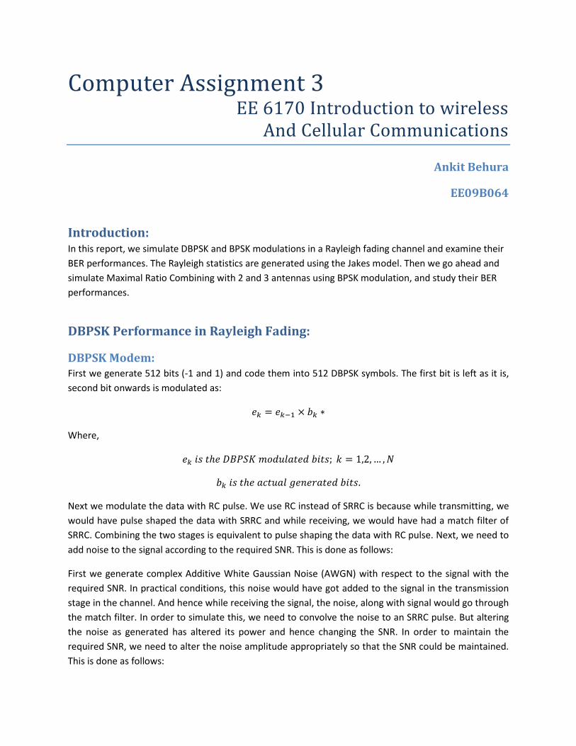
Figure 1: BER VS SNR plot of DBPSK in Rayleigh Fading

Observations: The simulated BER curve matches with the theoretical value for lower SNR. However for higher SNR, the

curves saturate. The curve with Doppler shift of 500Hz saturates first as expected as it will have more

errors than compared to that of 100Hz and 10Hz. The BER for 100Hz and 10Hz also saturate later.

Code: The code for the above section can be seen under the heading ‘Simulation of DBPSK in Rayleigh fading’, in the code section of the report.

BPSK Performance in Rayleigh Fading: Next we look at the performance of BPSK in Rayleigh fading. The bits generated are first converted to

BPSK, i.e. 1 is mapped to 1 and 0 is mapped to -1. This is then pulse shaped, passed through Jakes Model

of Rayleigh fading and added with noise exactly similar to that of described before. This represents BPSK

modulated received data passed through Rayleigh fading. A coherent detection now needs to be done

on this data. This is done by multiplying the data with the conjugate of the same Jakes coefficients.

Where,

This data is then thresholded to get back the sequence of 1 and -1. This is the decoded received data.

This is then compared with the actual bits generated, and the number of errors is accumulated and

averaged over 3000 such processes for each specified SNR (0 to 30 dB in steps of 2dB) and for each

specified Doppler shift (10Hz, 100Hz, 500Hz).

Theoretical BER for BPSK:

[ √

]

Where,

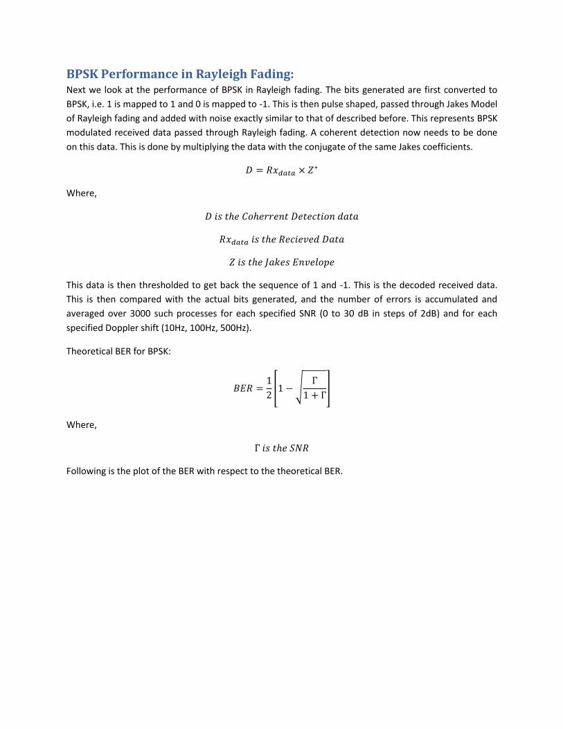
Following is the plot of the BER with respect to the theoretical BER.

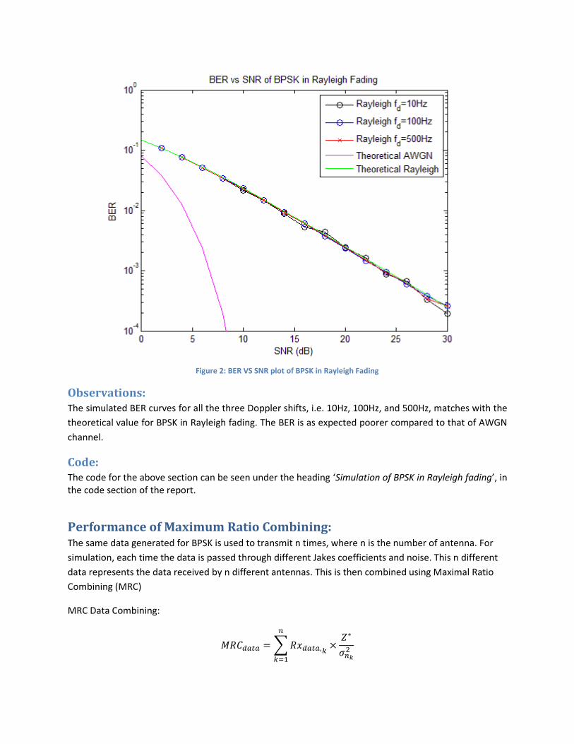
Figure 2: BER VS SNR plot of BPSK in Rayleigh Fading

Observations: The simulated BER curves for all the three Doppler shifts, i.e. 10Hz, 100Hz, and 500Hz, matches with the

theoretical value for BPSK in Rayleigh fading. The BER is as expected poorer compared to that of AWGN

channel.

Code: The code for the above section can be seen under the heading ‘Simulation of BPSK in Rayleigh fading’, in the code section of the report.

Performance of Maximum Ratio Combining: The same data generated for BPSK is used to transmit n times, where n is the number of antenna. For

simulation, each time the data is passed through different Jakes coefficients and noise. This n different

data represents the data received by n different antennas. This is then combined using Maximal Ratio

Combining (MRC)

MRC Data Combining:

∑

Where,

This MRC data is then thresholded to get the decoded data. This is then compared with the actual bits

generated, and the number of errors is accumulated and averaged over 3000 such processes for each

specified SNR (0 to 30 dB in steps of 2dB) and for each specified Doppler shift (10Hz, 100Hz, 500Hz).

Theoretical BER for MRC using BPSK in Rayleigh Fading:

[ ∑(

) (

)

(

)

]

Where,

√

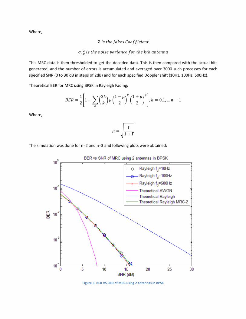
The simulation was done for n=2 and n=3 and following plots were obtained:

Figure 3: BER VS SNR of MRC using 2 antennas in BPSK

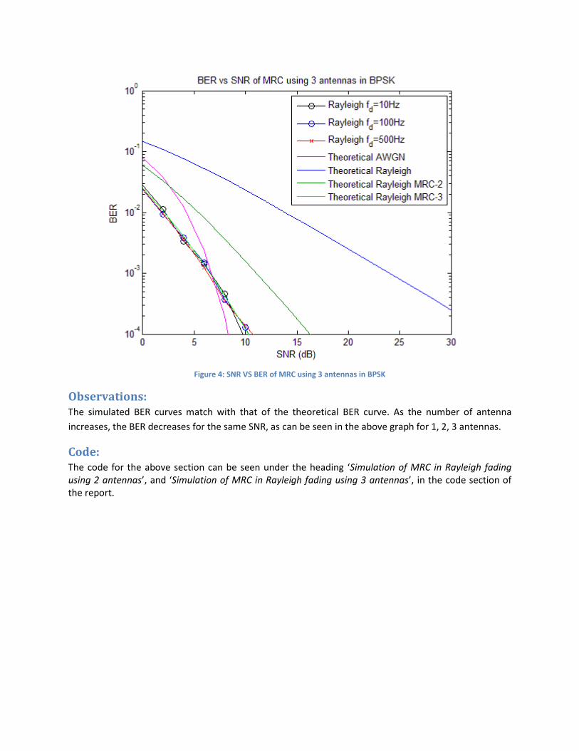
Figure 4: SNR VS BER of MRC using 3 antennas in BPSK

Observations: The simulated BER curves match with that of the theoretical BER curve. As the number of antenna

increases, the BER decreases for the same SNR, as can be seen in the above graph for 1, 2, 3 antennas.

Code: The code for the above section can be seen under the heading ‘Simulation of MRC in Rayleigh fading using 2 antennas’, and ‘Simulation of MRC in Rayleigh fading using 3 antennas’, in the code section of the report.

Code:

Generating SRRC Pulse: %% Generating SRRC pulse function srrc_pulse=srrc(w,a,T) s=size(w); srrc_pulse=zeros(1,s(2)); for k=1:s(2) t=w(k); if (t==0) srrc_pulse(k)=1-a+4*a/pi; elseif (t==T/(4*a) || t==(-T/(4*a))) srrc_pulse(k)=(a/sqrt(2))*((1+(2/pi))*sin(pi/(4*a))+(1-

(2/pi))*cos(pi/(4*a))); else srrc_pulse(k)=(sin(pi*(1-

a)*(t/T))+4*a*(t/T)*cos(pi*(1+a)*(t/T)))/(pi*(t/T)*(1-(4*a*(t/T))^2)); end end

Generating Rayleigh fading using Jakes Model: function Z=Jakes(fd,Tsample,t0,Num) % Z=Jakes( ) - returns fading waveform generated using Jakes’ model % fd= maximum Doppler frequency % Tsample= Time resolution of signal in seconds % t0 = starting time of oscillators % Num=Number of samples of fading to be generated N0=20; %Number of oscillators N=4*N0+2; %N is even but not multiple of 4 scale=2; %******************Modification 1: this line was not there in

previous program scale1=1/sqrt(scale*N0); %Scale factor for real part of fading channel scale2=1/sqrt(scale*(N0+1)); %Scale factor for imag part of fading channel n=1:N0; %Oscillator index t=(0:Tsample:(Num-1)*Tsample)+t0;%Time duration fn=fd*cos(2*pi*n/N); %fn – frequencies of oscillators in Jakes’ model alp=0; beta=n*pi/(N0+1); phi=2*pi*rand(N0,1); %Random phases for each oscillator ZC1=zeros(1,length(t)); ZS1=zeros(1,length(t)); for k=1:N0 %Real part ZC1=ZC1+2*cos(beta(k))*cos(2*pi*fn(k)*t+phi(k)); %Imag part ZS1=ZS1+2*sin(beta(k))*cos(2*pi*fn(k)*t+phi(k)); end ZC=(ZC1+sqrt(2)*cos(alp)*cos(2*pi*fd*t))*scale2; ZS=(ZS1+sqrt(2)*sin(alp)*cos(2*pi*fd*t))*scale1; Z=complex(ZC,ZS); % Z=Z/sqrt(var(Z)); %******************Modification 2:this line was there in % previous program end

Simulation of DBPSK in Rayleigh fading: %% DBPSK in Rayleigh Fading T=1/25000; oversam=8; num_symbols=10; w=-num_symbols/2:1/oversam:num_symbols/2; w=w*T; h1=srrc(w,0.35,T); rc=conv(h1,h1);

BER=zeros(3,16); Analytical_BER=zeros(1,16); A_BER_ray=zeros(1,16); doppler=[10,100,500]; for d=1:3 N=512; for snr=0:2:30 for count=1:3000 rand_bits=2*randint(1,N)-1; dbpsk_data=zeros(1,N); prevbit=1; for i = 1:N dbpsk_data(i)=rand_bits(i)*prevbit; prevbit=dbpsk_data(i); end pulshpd_data=conv(upsample(dbpsk_data,oversam),rc); pulshpd_data=downsample(pulshpd_data,oversam); pulshpd_data=pulshpd_data(11:end-10); noise1=awgn(pulshpd_data,snr)-pulshpd_data; noise2=awgn(pulshpd_data,snr)-pulshpd_data; noise=complex(noise1,noise2); noise=conv(upsample(noise,oversam),h1); noise=downsample(noise,oversam); noise=noise(6:end-5); p_s=sum(abs(pulshpd_data).^2); p_n=sum(abs(noise).^2); snr_n=10*log10(p_s/p_n); snr_r=snr; coeff=sqrt(10^((snr_r-snr_n)/10)); noise=noise/coeff; fade=Jakes(doppler(d),T,count*T*N*rand(),N); rx_data=pulshpd_data.*fade; rx_data=rx_data+noise;

decode_data=zeros(1,N); decode_data(1)=rx_data(1); decode_data(2:N)=rx_data(2:N).*conj(rx_data(1:N-1)); decode_data=sign(real(decode_data)); err=(rand_bits~=decode_data); BER(d,(snr/2)+1)=BER(d,(snr/2)+1)+sum(err);

end BER(d,(snr/2)+1)=BER(d,(snr/2)+1)/(N*3000); Analytical_BER((snr/2)+1)=(1/2)*exp(-1*10^(snr/10)); p=10^((snr)/10); A_BER_ray((snr/2)+1)=0.5/(1+p);

end d end

%% Plotting figure() semilogy(0:2:30,(BER(1,:)),'-ko',0:2:30,(BER(2,:)),'-bo',0:2:30,(BER(3,:)),'-

rx',0:2:30,(A_QPSK),'m',... 0:2:30,(A_BER_ray),'g'); title('BER vs SNR of DBPSK in Rayleigh Fading') xlabel('SNR (dB)') ylabel('BER') ylim([10^-4,1]); leg=legend('Rayleigh f_d=10Hz','Rayleigh f_d=100Hz','Rayleigh

f_d=500Hz','Theoretical AWGN',... 'Theoretical Rayleigh'); set(leg,'Location','NorthEast');

Simulation of BPSK in Rayleigh fading: %% BPSK in Rayleigh fading T=1/25000; oversam=8; num_symbols=10; w=-num_symbols/2:1/oversam:num_symbols/2; w=w*T; h1=srrc(w,0.35,T); rc=conv(h1,h1);

BER=zeros(3,16); A_BER_ray=zeros(1,16); A_QPSK=zeros(1,16); doppler=[10,100,500]; for d=1:3 N=512; for snr=0:2:30 for count=1:3000 rand_bits=2*randint(1,N)-1;

pulshpd_data=conv(upsample(rand_bits,oversam),rc); pulshpd_data=downsample(pulshpd_data,oversam); pulshpd_data=pulshpd_data(11:end-10); noise1=awgn(pulshpd_data,snr)-pulshpd_data; noise2=awgn(pulshpd_data,snr)-pulshpd_data; noise=complex(noise1,noise2); noise=conv(upsample(noise,oversam),h1); noise=downsample(noise,oversam); noise=noise(6:end-5); p_s=sum(abs(pulshpd_data).^2); p_n=sum(abs(noise).^2); snr_n=10*log10(p_s/p_n); snr_r=snr; coeff=sqrt(10^((snr_r-snr_n)/10)); noise=noise/coeff;

fade=Jakes(doppler(d),T,count*T*N*rand(),N); rx_data=pulshpd_data.*fade; rx_data=rx_data+noise;

rx_data=rx_data.*conj(fade); decode_data=sign(real(rx_data)); err=(rand_bits~=decode_data); BER(d,(snr/2)+1)=BER(d,(snr/2)+1)+sum(err);

end BER(d,(snr/2)+1)=BER(d,(snr/2)+1)/(N*3000); p=10^((snr)/10); A_BER_ray((snr/2)+1)=0.5*(1-sqrt(p/(1+p))); A_QPSK((snr/2)+1)=qfunc(sqrt(2*p)); end d end

%% Plotting figure() semilogy(0:2:30,(BER(1,:)),'-ko',0:2:30,(BER(2,:)),'-bo',0:2:30,(BER(3,:)),'-

rx',0:2:30,(A_QPSK),'m',... 0:2:30,(A_BER_ray),'g'); title('BER vs SNR of BPSK in Rayleigh Fading') xlabel('SNR (dB)') ylabel('BER') ylim([10^-4,1]); leg=legend('Rayleigh f_d=10Hz','Rayleigh f_d=100Hz','Rayleigh

f_d=500Hz','Theoretical AWGN',... 'Theoretical Rayleigh'); set(leg,'Location','NorthEast');

Simulation of MRC in Rayleigh fading using 2 antennas: %% BPSK in Rayleigh fading T=1/25000; oversam=8; num_symbols=10; w=-num_symbols/2:1/oversam:num_symbols/2; w=w*T; h1=srrc(w,0.35,T); rc=conv(h1,h1);

BER=zeros(3,16); A_BER_ray=zeros(1,16); A_QPSK=zeros(1,16); A_BER_ray_mrc2=zeros(1,16); doppler=[10,100,500]; for d=1:3 N=512; for snr=0:2:30 for count=1:3000 rand_bits=2*randint(1,N)-1;

pulshpd_data=conv(upsample(rand_bits,oversam),rc); pulshpd_data=downsample(pulshpd_data,oversam);

pulshpd_data=pulshpd_data(11:end-10);

noise1=awgn(pulshpd_data,snr)-pulshpd_data; noise2=awgn(pulshpd_data,snr)-pulshpd_data; noise=complex(noise1,noise2); noise=conv(upsample(noise,oversam),h1); noise=downsample(noise,oversam); noise=noise(6:end-5); p_s=sum(abs(pulshpd_data).^2); p_n=sum(abs(noise).^2); snr_n=10*log10(p_s/p_n); snr_r=snr; coeff=sqrt(10^((snr_r-snr_n)/10)); noise11=noise/coeff;

noise1=awgn(pulshpd_data,snr)-pulshpd_data; noise2=awgn(pulshpd_data,snr)-pulshpd_data; noise=complex(noise1,noise2); noise=conv(upsample(noise,oversam),h1); noise=downsample(noise,oversam); noise=noise(6:end-5); p_s=sum(abs(pulshpd_data).^2); p_n=sum(abs(noise).^2); snr_n=10*log10(p_s/p_n); snr_r=snr; coeff=sqrt(10^((snr_r-snr_n)/10)); noise22=noise/coeff;

fade1=Jakes(doppler(d),T,count*T*N*rand(),N); fade2=Jakes(doppler(d),T,count*T*N*rand(),N); rx_data1=pulshpd_data.*fade1+noise11; rx_data2=pulshpd_data.*fade2+noise22;

rx_data=rx_data1.*conj(fade1)/var(noise11)+rx_data2.*conj(fade2)/var(noise22)

; decode_data=sign(real(rx_data)); err=(rand_bits~=decode_data); BER(d,(snr/2)+1)=BER(d,(snr/2)+1)+sum(err);

end BER(d,(snr/2)+1)=BER(d,(snr/2)+1)/(N*3000); p=10^((snr)/10); A_BER_ray((snr/2)+1)=0.5*(1-sqrt(p/(1+p))); A_BER_ray_mrc2((snr/2)+1)=0.5*(1-sqrt(p/(1+p))-

((p/(1+p))^(3/2))/(2*p)); A_QPSK((snr/2)+1)=qfunc(sqrt(2*p)); end d end

%% Plotting figure() semilogy(0:2:30,(BER(1,:)),'-ko',0:2:30,(BER(2,:)),'-bo',0:2:30,(BER(3,:)),'-

rx',0:2:30,(A_QPSK),'m',... 0:2:30,(A_BER_ray),0:2:30,(A_BER_ray_mrc2),'g');

title('BER vs SNR of MRC using 2 antennas in BPSK') xlabel('SNR (dB)') ylabel('BER') ylim([10^-4,1]); leg=legend('Rayleigh f_d=10Hz','Rayleigh f_d=100Hz','Rayleigh

f_d=500Hz','Theoretical AWGN',... 'Theoretical Rayleigh','Theoretical Rayleigh MRC-2'); set(leg,'Location','NorthEast');

Simulation of MRC in Rayleigh fading using 3 antennas: %% BPSK in Rayleigh fading T=1/25000; oversam=8; num_symbols=10; w=-num_symbols/2:1/oversam:num_symbols/2; w=w*T; h1=srrc(w,0.35,T); rc=conv(h1,h1);

BER=zeros(3,16); A_BER_ray=zeros(1,16); A_QPSK=zeros(1,16); A_BER_ray_mrc2=zeros(1,16); A_BER_ray_mrc3=zeros(1,16); doppler=[10,100,500]; for d=1:3 N=512; for snr=0:2:30 for count=1:3000 rand_bits=2*randint(1,N)-1;

pulshpd_data=conv(upsample(rand_bits,oversam),rc); pulshpd_data=downsample(pulshpd_data,oversam); pulshpd_data=pulshpd_data(11:end-10);

noise1=awgn(pulshpd_data,snr)-pulshpd_data; noise2=awgn(pulshpd_data,snr)-pulshpd_data; noise=complex(noise1,noise2); noise=conv(upsample(noise,oversam),h1); noise=downsample(noise,oversam); noise=noise(6:end-5); p_s=sum(abs(pulshpd_data).^2); p_n=sum(abs(noise).^2); snr_n=10*log10(p_s/p_n); snr_r=snr; coeff=sqrt(10^((snr_r-snr_n)/10)); noise11=noise/coeff;

noise1=awgn(pulshpd_data,snr)-pulshpd_data; noise2=awgn(pulshpd_data,snr)-pulshpd_data; noise=complex(noise1,noise2); noise=conv(upsample(noise,oversam),h1); noise=downsample(noise,oversam); noise=noise(6:end-5);

p_s=sum(abs(pulshpd_data).^2); p_n=sum(abs(noise).^2); snr_n=10*log10(p_s/p_n); snr_r=snr; coeff=sqrt(10^((snr_r-snr_n)/10)); noise22=noise/coeff;

noise1=awgn(pulshpd_data,snr)-pulshpd_data; noise2=awgn(pulshpd_data,snr)-pulshpd_data; noise=complex(noise1,noise2); noise=conv(upsample(noise,oversam),h1); noise=downsample(noise,oversam); noise=noise(6:end-5); p_s=sum(abs(pulshpd_data).^2); p_n=sum(abs(noise).^2); snr_n=10*log10(p_s/p_n); snr_r=snr; coeff=sqrt(10^((snr_r-snr_n)/10)); noise33=noise/coeff;

fade1=Jakes(doppler(d),T,count*T*N*rand(),N); fade2=Jakes(doppler(d),T,count*T*N*rand(),N); fade3=Jakes(doppler(d),T,count*T*N*rand(),N); rx_data1=pulshpd_data.*fade1+noise11; rx_data2=pulshpd_data.*fade2+noise22; rx_data3=pulshpd_data.*fade3+noise33;

rx_data=rx_data1.*conj(fade1)/var(noise11)+rx_data2.*conj(fade2)/var(noise22)

+rx_data3.*conj(fade3)/var(noise33); decode_data=sign(real(rx_data)); err=(rand_bits~=decode_data); BER(d,(snr/2)+1)=BER(d,(snr/2)+1)+sum(err);

end BER(d,(snr/2)+1)=BER(d,(snr/2)+1)/(N*3000); p=10^((snr)/10); A_BER_ray((snr/2)+1)=0.5*(1-sqrt(p/(1+p))); A_BER_ray_mrc2((snr/2)+1)=0.5*(1-sqrt(p/(1+p))-

((p/(1+p))^(3/2))/(2*p)); A_QPSK((snr/2)+1)=qfunc(sqrt(2*p)); A_BER_ray_mrc3((snr/2)+1)=0.5*(1-sqrt(p/(1+p))-

((p/(1+p))^(3/2))/(2*p)-3*((p/(1+p))^(5/2))/(8*p^2)); end d end

%% Plotting figure() semilogy(0:2:30,(BER(1,:)),'-ko',0:2:30,(BER(2,:)),'-bo',0:2:30,(BER(3,:)),'-

rx',0:2:30,(A_QPSK),'m',... 0:2:30,(A_BER_ray),0:2:30,(A_BER_ray_mrc2),0:2:30,(A_BER_ray_mrc3),'g'); title('BER vs SNR of MRC using 3 antennas in BPSK') xlabel('SNR (dB)') ylabel('BER') ylim([10^-4,1]);

leg=legend('Rayleigh f_d=10Hz','Rayleigh f_d=100Hz','Rayleigh

f_d=500Hz','Theoretical AWGN',... 'Theoretical Rayleigh','Theoretical Rayleigh MRC-2','Theoretical Rayleigh

MRC-3'); set(leg,'Location','NorthEast');

I certify that this assignment submission is my own work and not obtained from any other

source

X Ankit Behura

Ankit Behura

EE09B064

Signed by: Ankit Behura