Commonness and rarity in the marine biosphere

Page 1

Commonness and rarity in the marine biosphereSean R. Connollya,1, M. Aaron MacNeilb, M. Julian Caleyb, Nancy Knowltonc,1, Ed Crippsd, Mizue Hisanoa,Loïc M. Thibauta, Bhaskar D. Bhattacharyae, Lisandro Benedetti-Cecchif, Russell E. Brainardg, Angelika Brandth,Fabio Bullerif, Kari E. Ellingseni, Stefanie Kaiserj, Ingrid Krönckek, Katrin Linsel, Elena Maggif, Timothy D. O’Haram,Laetitia Plaisancec, Gary C. B. Poorem, Santosh K. Sarkare, Kamala K. Satpathyn, Ulrike Schückelk, Alan Williamso,and Robin S. Wilsonm

aSchool of Marine and Tropical Biology, and Australian Research Council Centre of Excellence for Coral Reef Studies, James Cook University, Townsville, QLD4811, Australia; bAustralian Institute of Marine Science, Townsville, QLD 4810, Australia; cNational Museum of Natural History, Smithsonian Institution,Washington, DC 20013; dSchool of Mathematics and Statistics, University of Western Australia, Perth, WA 6009, Australia; eDepartment of Marine Science,University of Calcutta, Calcutta 700 019, India; fDipartimento di Biologia, University of Pisa, I-56126 Pisa, Italy; gCoral Reef Ecosystem Division, Pacific IslandsFisheries Science Center, National Oceanic and Atmospheric Administration, Honolulu, HI 96818; hBiocenter Grindel and Zoological Museum, University ofHamburg, 20146 Hamburg, Germany; iNorwegian Institute for Nature Research, FRAM–High North Research Centre for Climate and the Environment, 9296Tromsø, Norway; jGerman Centre for Marine Biodiversity Research, Senckenberg am Meer, 26382 Wilhelmshaven, Germany; kMarine Research Department,Senckenberg am Meer, 26382 Wilhelmshaven, Germany; lBritish Antarctic Survey, Cambridge CB3 0ET, United Kingdom; mMuseum Victoria, Melbourne, VIC3001, Australia; nEnvironment and Safety Division, Indira Gandhi Centre for Atomic Research, Kalpakkam 603 102, India; and oCommonwealth Scientificand Industrial Research Organization, Marine and Atmospheric Research, Marine Laboratories, Hobart, TAS 7001, Australia

Contributed by Nancy Knowlton, April 28, 2014 (sent for review November 25, 2013; reviewed by Brian McGill and Fangliang He)

Explaining patterns of commonness and rarity is fundamental forunderstanding and managing biodiversity. Consequently, a keytest of biodiversity theory has been how well ecological modelsreproduce empirical distributions of species abundances. However,ecological models with very different assumptions can predictsimilar species abundance distributions, whereas models withsimilar assumptions may generate very different predictions. Thiscomplicates inferring processes driving community structure frommodel fits to data. Here, we use an approximation that capturescommon features of “neutral” biodiversity models—which assumeecological equivalence of species—to test whether neutrality isconsistent with patterns of commonness and rarity in the marinebiosphere. We do this by analyzing 1,185 species abundance dis-tributions from 14 marine ecosystems ranging from intertidalhabitats to abyssal depths, and from the tropics to polar regions.Neutrality performs substantially worse than a classical nonneu-tral alternative: empirical data consistently show greater hetero-geneity of species abundances than expected under neutrality.Poor performance of neutral theory is driven by its consistent in-ability to capture the dominance of the communities’ most-abun-dant species. Previous tests showing poor performance of a neutralmodel for a particular system often have been followed by contro-versy about whether an alternative formulation of neutral theorycould explain the data after all. However, our approach focuses oncommon features of neutral models, revealing discrepancies witha broad range of empirical abundance distributions. These findingshighlight the need for biodiversity theory in which ecological differ-ences among species, such as niche differences and demographictrade-offs, play a central role.

metacommunities | marine macroecology | species coexistence |Poisson-lognormal distribution

Determining how biodiversity is maintained in ecologicalcommunities is a long-standing ecological problem. In

species-poor communities, niche and demographic differencesbetween species can often be estimated directly and used to inferthe importance of alternative mechanisms of species coexistence(1–3). However, the “curse of dimensionality” prevents the ap-plication of such species-by-species approaches to high-diversityassemblages: the number of parameters in community dynamicsmodels increases more rapidly than the amount of data, as speciesrichness increases. Moreover, most species in high-diversityassemblages are very rare, further complicating the estimation ofstrengths of ecological interactions among species, or covariationin different species’ responses to environmental fluctuations.Consequently, ecologists have focused instead on making assump-tions about the overall distribution of demographic rates, niche

sizes, or other characteristics of an assemblage, and then de-riving the aggregate assemblage properties implied by thoseassumptions (4–8). One of the most commonly investigated ofthese assemblage-level properties is the species abundance distri-bution (SAD)—the pattern of commonness and rarity amongspecies (9–11). Ecologists have long sought to identifymechanismsthat can explain common features of, and systematic differencesamong, the shapes of such distributions, and have used the abilityto reproduce empirical SADs as a key test of biodiversity theory inspecies-rich systems (4, 6, 11–14).Over the last decade, one of the most prevalent and influential

approaches to explaining the structure of high-diversity assemb-lages has been neutral theory of biodiversity (12, 15, 16). Neutralmodels assume that individuals are demographically and ecologi-cally equivalent, regardless of species. Thus, variation in relative

Significance

Tests of biodiversity theory have been controversial partlybecause alternative formulations of the same theory seeminglyyield different conclusions. This has been a particular challengefor neutral theory, which has dominated tests of biodiversitytheory over the last decade. Neutral theory attributes differ-ences in species abundances to chance variation in individuals’fates, rather than differences in species traits. By identifyingcommon features of different neutral models, we conduct auniquely robust test of neutral theory across a global datasetof marine assemblages. Consistently, abundances vary moreamong species than neutral theory predicts, challenging thehypothesis that community dynamics are approximately neu-tral, and implicating species differences as a key driver ofcommunity structure in nature.

Author contributions: S.R.C., M.A.M., and M.J.C. designed research; N.K., B.D.B., L.B.-C.,R.E.B., A.B., F.B., K.E.E., S.K., I.K., K.L., E.M., T.D.O., L.P., G.C.B.P., S.K.S., K.K.S., U.S.,A.W., and R.S.W. performed research; S.R.C., E.C., M.H., and L.M.T. analyzed data; S.R.C.designed analytical approach; M.J.C. initiated the collaboration between Census ofMarine Life and S.R.C.; N.K. was the initiator of Census of Marine Life Project (producerof dataset) for coral reefs; N.K. designed data collection protocols; B.D.B., L.B.-C.,R.E.B., A.B., F.B., K.E.E., S.K., I.K., K.L., E.M., T.D.O., L.P., G.C.B.P., S.K.S., K.K.S., U.S.,A.W., and R.S.W. provided advice on treatment of data for analyses; and S.R.C.,M.A.M., M.J.C., N.K., and E.C. wrote the paper.

Reviewers: B.M., University of Maine; F.H., University of Alberta.

The authors declare no conflict of interest.

Freely available online through the PNAS open access option.1To whom correspondence may be addressed. E-mail: [email protected] or [email protected].

This article contains supporting information online at www.pnas.org/lookup/suppl/doi:10.1073/pnas.1406664111/-/DCSupplemental.

www.pnas.org/cgi/doi/10.1073/pnas.1406664111 PNAS Early Edition | 1 of 6

ECOLO

GY

Page 2

abundance among species arises purely from demographic sto-chasticity: chance variation in the fates of individuals (i.e., birth,death, immigration, and speciation events). Most studies in-vestigating neutral theory aim to determine whether communitystructure in nature is consistent with the theory’s core speciesequivalence assumption. This is typically done by assessing the fitof a neutral model to empirical data, sometimes relative to aputatively nonneutral alternative (17–20). However, although allneutral models share the species equivalence assumption, theydiffer with respect to auxiliary assumptions, such as the mode ofspeciation assumed, leading to different predictions for SADs andother ecological patterns. Indeed, attempts to draw conclusionsfrom tests of neutral theory are almost invariably disputed, largelydue to arguments about the extent to which alternative auxiliaryassumptions can materially alter neutral theory’s ability to explainthe data (11, 12, 18, 21).An alternative, potentially more robust approach to evaluating

neutral theory was proposed by Pueyo (22), based on approxi-mating neutral and nonneutral dynamics as successively higher-order perturbations of a model for the idealized case of purerandom drift in abundances. This approach predicts that a gamma

distribution should approximate the distribution of species abun-dances for small departures for random drift, whereas assemblagesexhibiting greater departures from neutrality should be betterapproximated by a lognormal distribution. This raises the possi-bility that a comparison of gamma and lognormal SADs could offera robust test for the signature of nonneutrality in species abun-dance data, provided that the gamma distribution provides a suffi-ciently close approximation to SADs produced by neutral models.Here, we evaluate Pueyo’s framework and apply it to patterns

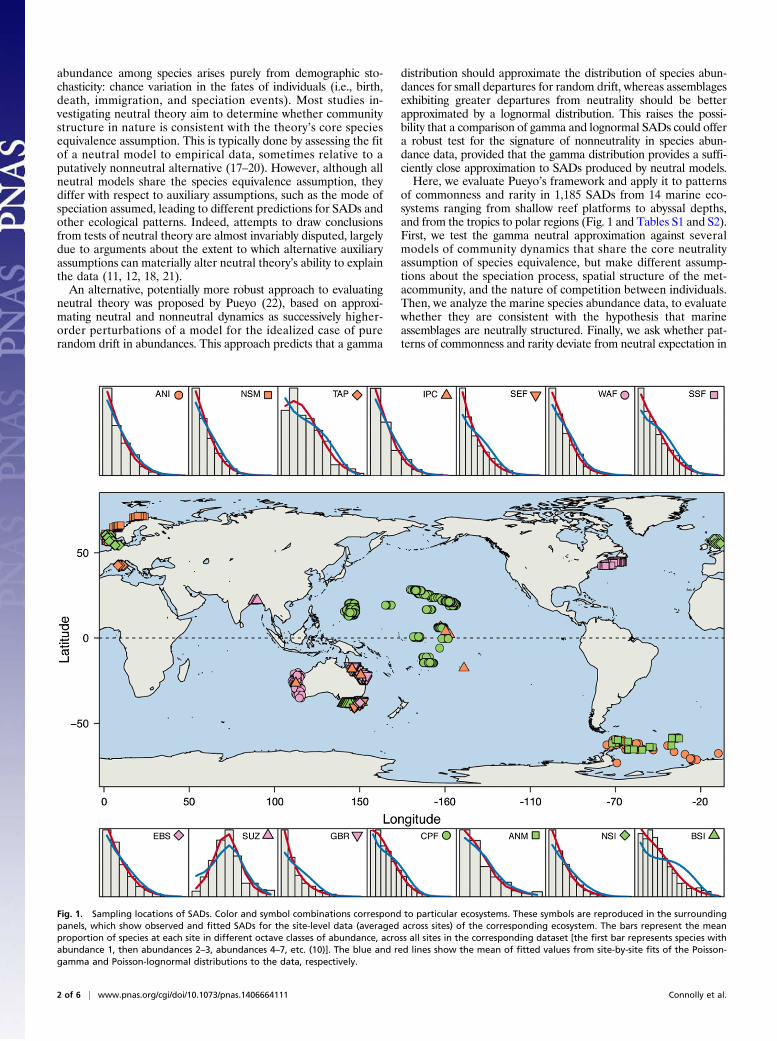
of commonness and rarity in 1,185 SADs from 14 marine eco-systems ranging from shallow reef platforms to abyssal depths,and from the tropics to polar regions (Fig. 1 and Tables S1 and S2).First, we test the gamma neutral approximation against severalmodels of community dynamics that share the core neutralityassumption of species equivalence, but make different assump-tions about the speciation process, spatial structure of the met-acommunity, and the nature of competition between individuals.Then, we analyze the marine species abundance data, to evaluatewhether they are consistent with the hypothesis that marineassemblages are neutrally structured. Finally, we ask whether pat-terns of commonness and rarity deviate from neutral expectation in

Fig. 1. Sampling locations of SADs. Color and symbol combinations correspond to particular ecosystems. These symbols are reproduced in the surroundingpanels, which show observed and fitted SADs for the site-level data (averaged across sites) of the corresponding ecosystem. The bars represent the meanproportion of species at each site in different octave classes of abundance, across all sites in the corresponding dataset [the first bar represents species withabundance 1, then abundances 2–3, abundances 4–7, etc. (10)]. The blue and red lines show the mean of fitted values from site-by-site fits of the Poisson-gamma and Poisson-lognormal distributions to the data, respectively.

2 of 6 | www.pnas.org/cgi/doi/10.1073/pnas.1406664111 Connolly et al.

Page 3

idiosyncratic ways, or whether there are particular features of realSADs that cannot be captured by neutral models.

ResultsA gamma distribution of species abundances closely approx-imates several alternative neutral models across a broad range ofneutral model parameter values (Fig. S1; see SI Results for fur-ther discussion). Moreover, the gamma consistently outperformsthe lognormal when fitted to data simulated from neutral mod-els. Specifically, as the number of distinct species abundancevalues in the simulated data increases, the relative support forthe gamma distribution becomes consistently stronger for all ofthe neutral models we considered (Fig. 2A). This reflects the factthat datasets with only a small number of abundance values (e.g.,a site containing 11 species, 10 of which are only represented byone individual) provide very little information about the shape ofthe SAD, whereas those with more abundance values providemore information (e.g., a site with 100 species whose abundancesare spread over 10–20 different values).In contrast to their relative fit to simulated neutral SADs, the

lognormal consistently outperforms the gamma distributionwhen fitted to real marine species abundance data. When con-sidered in terms of average support per SAD, relative support forthe lognormal becomes consistently stronger as the number ofobserved species abundance values increases, in direct contrastwith the simulated neutral data (Fig. 2B). Moreover, when thestrength of evidence is considered cumulatively across all sitesfor each dataset, the lognormal has well over 99% support as thebetter model in each case (Table 1). This substantially better fitof the lognormal is retained in every case when data are pooledto the mesoscale, and, in all cases save one, when data are pooledat the regional scale (Table 1, Fig. 2B, and Figs. S2 and S3). Thelognormal also remained strongly favored when we tested therobustness of our results by classifying species into taxonomicand ecological guilds, and restricting our analysis to the mostspecies-rich guild within each dataset (see SI Results and Table S3).Inspection of the lack of fit of the gamma neutral approxi-

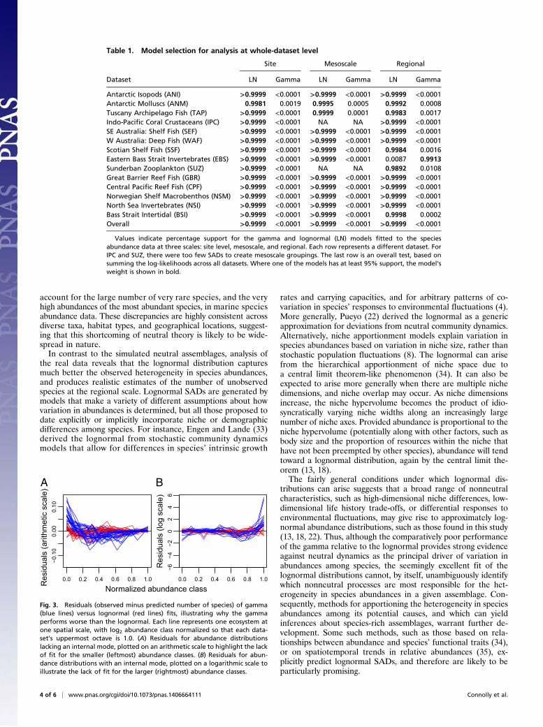
mation indicates that it deviates from the data in highly consis-tent ways: real SADs exhibit substantially more heterogeneitythan the gamma distribution can generate (Fig. 3). Specifically,the gamma is unable to simultaneously capture the large numberof rare species and the very high abundances of the most common

species. For abundance distributions lacking an internal mode(i.e., where the leftmost bar in the SAD is the largest one), this ismanifested as an excess of rare species and paucity of species withintermediate abundance, relative to the best-fit neutral approxi-mation (Fig. 3A, blue lines). Conversely, when an internal mode ispresent in the data, the abundances of the most highly abundantspecies are consistently higher than the gamma distribution canproduce (Fig. 3B, blue lines). In contrast, discrepancies betweenthe data and the lognormal are much smaller in magnitude, andmore symmetrically distributed around zero, compared with thegamma (Fig. 3, red lines).Detailed analysis of variation in the strength of evidence

against neutrality, within and among datasets, indicates that therelative performance of the lognormal over the gamma is sub-stantially driven by the fact that the most abundant species is, onaverage, too dominant to be captured by the gamma neutralapproximation. After controlling for the effects of the number ofabundance values in the sample on statistical power, the relativeabundance of the most-abundant species explained over one-halfof the variation in the strength of support for the lognormal overthe gamma, for site-level, mesoscale, and regional-scale abun-dance distributions (Table S4, Fig. S4, and SI Results). Con-versely, the prevalence of rarity was a poor predictor of the strengthof evidence against the gamma neutral approximation (Table S4,Fig. S5, and SI Results).In addition to outperforming the gamma neutral approxima-

tion, tests of the absolute goodness of fit of the lognormal sug-gest that it approximates the observed species abundance datawell. Statistically significant lack of fit (at α = 0.05) to the log-normal was detected in 4.8% of sites, approximately equal towhat would be expected by chance, under the null hypothesisthat the SADs are in fact lognormal. Moreover, lognormal-basedestimates of the number of unobserved species in the regionalspecies pool are realistic, and very similar to those produced byan alternative, nonparametric jackknife method that relies onpresence–absence rather than abundance data (Fig. 4).

DiscussionRecently, the use of SADs to test biodiversity theory has beencriticized because different species abundance models oftengenerate very similar predictions, which can be difficult to dis-tinguish when fitted to species abundance data (9). Conse-quently, some researchers have focused on other properties ofassemblages, such as community similarity (12), species–area andspecies–time relationships (23, 24), and relationships betweenspecies traits or phylogeny and species abundance (25, 26). Suchapproaches are powerful when evaluating the performance ofparticular species abundance models. However, because modelscombine multiple assumptions, attributing a model’s failure toone assumption in particular, such as species equivalence, isproblematic. Indeed, in the debate over neutral theory of bio-diversity, studies that show failure of a neutral model (12, 25, 27)are almost invariably followed by responses showing that pack-aging neutrality with a different set of alternative assumptionscan explain the data after all (11, 28, 29). Although the identifi-cation of alternative auxiliary assumptions that preserve a theory’score prevents premature abandonment of a promising theory, italso can hinder progress by inhibiting the reallocation of scientificeffort to more promising research programs (30). Given the pro-liferation of alternative theories of biodiversity (8, 14, 31, 32),identifying and testing predictions that are robust to auxiliaryassumptions, and therefore better target a theory’s core assump-tions, should be a high priority.Here, we showed that, as previously hypothesized (22), a

gamma distribution successfully captures features common toseveral models that share the core neutrality assumptions of spe-cies equivalence, but make very different auxiliary assumptions.We then found that this approximation cannot simultaneously

10 20 50 100 200

0.0

0.4

0.8

A

OriginalFissionProtracted

IndependentSpatial

10 20 50 100 200

B

ANIANMBSI

CPFEBSGBR

IPCNSINSM

SEFSSFSUZ

TAPWAF

Median number of distinct abundance values

Mea

n A

kaik

e w

eigh

t for

logn

orm

al o

ver g

amm

a

SiteMesoRegional

Fig. 2. Species abundances are better approximated by (A) a gamma dis-tribution for simulated neutral communities, but (B) a lognormal distribu-tion for the empirical data. Percentage support for the lognormal versus thegamma is plotted as a function of the number of observed distinct speciesabundances. In A, different neutral models are plotted with different colors,and each point represents a particular neutral model parameter combina-tion from Fig. S1. In B, each combination of symbol and color representsa different marine ecosystem, whereas increasing symbol size indicates the in-creasing scale at which abundances were pooled (site, mesoscale, and regional).

Connolly et al. PNAS Early Edition | 3 of 6

ECOLO

GY

Page 4

account for the large number of very rare species, and the veryhigh abundances of the most abundant species, in marine speciesabundance data. These discrepancies are highly consistent acrossdiverse taxa, habitat types, and geographical locations, suggest-ing that this shortcoming of neutral theory is likely to be wide-spread in nature.In contrast to the simulated neutral assemblages, analysis of

the real data reveals that the lognormal distribution capturesmuch better the observed heterogeneity in species abundances,and produces realistic estimates of the number of unobservedspecies at the regional scale. Lognormal SADs are generated bymodels that make a variety of different assumptions about howvariation in abundances is determined, but all those proposed todate explicitly or implicitly incorporate niche or demographicdifferences among species. For instance, Engen and Lande (33)derived the lognormal from stochastic community dynamicsmodels that allow for differences in species’ intrinsic growth

rates and carrying capacities, and for arbitrary patterns of co-variation in species’ responses to environmental fluctuations (4).More generally, Pueyo (22) derived the lognormal as a genericapproximation for deviations from neutral community dynamics.Alternatively, niche apportionment models explain variation inspecies abundances based on variation in niche size, rather thanstochastic population fluctuations (8). The lognormal can arisefrom the hierarchical apportionment of niche space due toa central limit theorem-like phenomenon (34). It can also beexpected to arise more generally when there are multiple nichedimensions, and niche overlap may occur. As niche dimensionsincrease, the niche hypervolume becomes the product of idio-syncratically varying niche widths along an increasingly largenumber of niche axes. Provided abundance is proportional to theniche hypervolume (potentially along with other factors, such asbody size and the proportion of resources within the niche thathave not been preempted by other species), abundance will tendtoward a lognormal distribution, again by the central limit the-orem (13, 18).The fairly general conditions under which lognormal dis-

tributions can arise suggests that a broad range of nonneutralcharacteristics, such as high-dimensional niche differences, low-dimensional life history trade-offs, or differential responses toenvironmental fluctuations, may give rise to approximately log-normal abundance distributions, such as those found in this study(13, 18, 22). Thus, although the comparatively poor performanceof the gamma relative to the lognormal provides strong evidenceagainst neutral dynamics as the principal driver of variation inabundances among species, the seemingly excellent fit of thelognormal distributions cannot, by itself, unambiguously identifywhich nonneutral processes are most responsible for the het-erogeneity in species abundances in a given assemblage. Con-sequently, methods for apportioning the heterogeneity in speciesabundances among its potential causes, and which can yieldinferences about species-rich assemblages, warrant further de-velopment. Some such methods, such as those based on rela-tionships between abundance and species’ functional traits (34),or on spatiotemporal trends in relative abundances (35), ex-plicitly predict lognormal SADs, and therefore are likely to beparticularly promising.

Table 1. Model selection for analysis at whole-dataset level

Site Mesoscale Regional

Dataset LN Gamma LN Gamma LN Gamma

Antarctic Isopods (ANI) >0.9999 <0.0001 >0.9999 <0.0001 >0.9999 <0.0001Antarctic Molluscs (ANM) 0.9981 0.0019 0.9995 0.0005 0.9992 0.0008Tuscany Archipelago Fish (TAP) >0.9999 <0.0001 0.9999 0.0001 0.9983 0.0017Indo-Pacific Coral Crustaceans (IPC) >0.9999 <0.0001 NA NA >0.9999 <0.0001SE Australia: Shelf Fish (SEF) >0.9999 <0.0001 >0.9999 <0.0001 >0.9999 <0.0001W Australia: Deep Fish (WAF) >0.9999 <0.0001 >0.9999 <0.0001 >0.9999 <0.0001Scotian Shelf Fish (SSF) >0.9999 <0.0001 >0.9999 <0.0001 0.9984 0.0016Eastern Bass Strait Invertebrates (EBS) >0.9999 <0.0001 >0.9999 <0.0001 0.0087 0.9913Sunderban Zooplankton (SUZ) >0.9999 <0.0001 NA NA 0.9892 0.0108Great Barrier Reef Fish (GBR) >0.9999 <0.0001 >0.9999 <0.0001 >0.9999 <0.0001Central Pacific Reef Fish (CPF) >0.9999 <0.0001 >0.9999 <0.0001 >0.9999 <0.0001Norwegian Shelf Macrobenthos (NSM) >0.9999 <0.0001 >0.9999 <0.0001 >0.9999 <0.0001North Sea Invertebrates (NSI) >0.9999 <0.0001 >0.9999 <0.0001 >0.9999 <0.0001Bass Strait Intertidal (BSI) >0.9999 <0.0001 >0.9999 <0.0001 0.9998 0.0002Overall >0.9999 <0.0001 >0.9999 <0.0001 >0.9999 <0.0001

Values indicate percentage support for the gamma and lognormal (LN) models fitted to the speciesabundance data at three scales: site level, mesoscale, and regional. Each row represents a different dataset. ForIPC and SUZ, there were too few SADs to create mesoscale groupings. The last row is an overall test, based onsumming the log-likelihoods across all datasets. Where one of the models has at least 95% support, the model’sweight is shown in bold.

0.0 0.2 0.4 0.6 0.8 1.0

−0.1

00.

000.

10R

esid

uals

(arit

hmet

ic s

cale

)A

0.0 0.2 0.4 0.6 0.8 1.0

−6−4

−20

24

6R

esid

uals

(log

sca

le)

B

Normalized abundance class

Fig. 3. Residuals (observed minus predicted number of species) of gamma(blue lines) versus lognormal (red lines) fits, illustrating why the gammaperforms worse than the lognormal. Each line represents one ecosystem atone spatial scale, with log2 abundance class normalized so that each data-set’s uppermost octave is 1.0. (A) Residuals for abundance distributionslacking an internal mode, plotted on an arithmetic scale to highlight the lackof fit for the smaller (leftmost) abundance classes. (B) Residuals for abun-dance distributions with an internal mode, plotted on a logarithmic scale toillustrate the lack of fit for the larger (rightmost) abundance classes.

4 of 6 | www.pnas.org/cgi/doi/10.1073/pnas.1406664111 Connolly et al.

Page 5

ConclusionsNeutral theory explains variation in the abundances and distribu-tion of species entirely as a consequence of demographic sto-chasticity—chance variation in the fates of individuals (15, 36).Although proponents of neutral theory have always acknowledgedthe existence of ecological differences between species, neutraltheory assumes that those differences are overwhelmed by thephenomena that are explicitly included in neutral models (14, 36).The formulation and testing of neutral theory has drawn attentionto the potential importance of demographic stochasticity as aprocess that contributes to differences in species abundances thatare unrelated to species’ ecological traits, such as niche size orcompetitive ability. Such effects should be particularly importantamong rare species (4). Indeed, our finding that there are commonfeatures of different neutral models suggests that it can play a roleas a robust null expectation, at least for some aspects of commu-nity structure (16). However, the most abundant few species oftennumerically dominate communities and play a disproportionatelylarge role in community and ecosystem processes (37). We haveshown that neutral theory consistently underestimates among-species heterogeneity in abundances across a broad range ofmarine systems. The fact that its performance is closely linked toabundances of the most common species indicates that it is theecological dominance of these very highly abundant species thatcannot be explained by neutral processes alone. Commonnessitself is poorly understood, but the identities of the most commonspecies in ecosystems tend to remain quite consistent over eco-logical timescales (38). Thus, the key to understanding the distri-bution of abundances in communities, even species-rich ones, maylie as much in understanding how the characteristics of commonspecies allow them to remain so abundant, as in understanding thedynamics and persistence of rare species.

Materials and MethodsApproximating Neutrality. Pueyo’s framework starts with a stochastic differ-ential equation for random drift in population size (i.e., birth rate equalsdeath rate, no density dependence, immigration, emigration, or speciation)and considers approximating departures from this model in terms of succes-sively higher-order perturbations to it. Here, we take as our candidate neutralapproximation the gamma distribution and, as our alternative model, thelognormal distribution. More specifically, because species abundance data arediscrete, whereas the gamma and lognormal are continuous distributions, weuse the Poisson-gamma (i.e., negative binomial) and Poisson-lognormal mix-ture distributions, as these distributions are commonly used to approximatediscrete, random samples from underlying gamma or lognormal communityabundance distributions (see SI Materials and Methods for further details).

To assess whether the Poisson-gamma distribution provides a good ap-proximation to the SADs produced under neutrality, we tested it against five

different neutral models: Hubbell’s original neutral model (39), a protractedspeciation neutral model (21), a fission speciation model (40), an independentspecies model (11, 41), and a spatially explicit neutral model (42). We chosethese five models because they encompass models that relax key assumptionsof neutral theory as originally formulated; moreover, each of them meetsa strict definition of neutrality: every individual has the same demographicrates, and the same per-capita effects on other individuals, regardless ofspecies. We tested the approximation in twoways. First, we assess how closely(in absolute terms) the Poisson-gamma can approximate neutral abundancedistributions. Second, we assess whether the Poisson-gamma outperforms thePoisson-lognormal when fitted to data generated according to neutral modelassumptions (see SI Materials and Methods for details).

Empirical Data. Data were contributed to the Census of Marine Life (CoML)project and represent a diverse range of taxa, ocean realms, depths, andgeographic locations (Table S1). To be included in our analysis, contributeddata needed to meet several criteria (see SI Materials and Methods fordetails). Where datasets included samples over multiple years from the samesites, only the most recent year of data was used. Finally, we only fitted SADsif they contained more than five distinct species abundance values, tominimize convergence problems associated with fitting species abundancemodels to very sparse data. However, the data from such sites were still usedin the analyses that pooled abundance distributions at larger scales.

Fitting Models to Species Abundance Data. For both the simulated neutraldata, and the real species abundance data, we fitted our models usingmaximum-likelihood methods (see SI Materials and Methods for details). Forthe empirical data, in addition to fitting our species abundance models atthe site level, we also fitted pooled species abundances at a mesoscale level,and at the regional (whole-dataset) level. For datasets that were spatiallyhierarchically organized, we used this hierarchy to determine how to poolsites at the mesoscale [e.g., for the Central Pacific Reef Fish (CPF) data, siteswere nested within islands, so pooling was done to the island level]. For datathat were not explicitly hierarchically organized [Antarctic Isopods (ANI),Antarctic Molluscs (ANM), Scotian Shelf Fish (SSF), Bass Strait Intertidal (BSI)],cluster analysis was used to identify mesoscale-level groupings. In two cases[Sunderban Zooplankton (SUZ), Indo-Pacific Coral Crustaceans (IPC)], therewere only a few sites sampled, and no natural hierarchical structure, so thesedata were omitted from the mesoscale analysis.

For both the analysis of the marine species abundance data, and theanalysis of the simulated neutral communities, model selection was basedon Akaike weights, which are calculated from Akaike’s information criterionvalues and estimate the probability (expressed on a scale of 0–1) thata model is actually the best approximating model in the set being consid-ered. Because the Poisson-gamma and the Poisson-lognormal have the samenumber of estimated parameters, this is equivalent to calculating modelweights based on the Bayesian information criterion. For the empirical data,model selection was done at the whole-dataset level by summing the log-likelihoods for all individual sites (for the site-level analysis) or mesoscale (forthe mesoscale analysis) abundance distributions for a dataset, and calculat-ing Akaike weights based on these values (Table 1). However, this approachdoes not make sense for the analysis of the simulated neutral SADs, becausean arbitrary degree of confidence can be obtained by simulating a largenumber of sites. Therefore, we instead calculated an expected level of modelsupport on a per-SAD basis, for each neutral model and parameter combi-nation, by calculating the mean difference in log-likelihoods across the 100simulated datasets, and converting this mean into an Akaike weight. Weexamined these Akaike weights as functions of the number of distinct ob-served species abundance values, because we would expect our ability todistinguish between alternative models to increase as the number of distinctobserved species abundance values increases. For comparison, we also cal-culated per-SAD Akaike weights for the marine species abundance data. Thisapproach is less powerful than the aggregate whole-dataset comparisonsshown in Table 1, but it facilitates visualization of the differences betweenthe simulated neutral SADs (Fig. 2A) and the real marine SADs (Fig. 2B).

Analysis of Variation in Performance of Neutral Approximation. The discrep-ancies between the data and the gamma neutral approximation suggest thatreal data exhibit too much heterogeneity in species’ abundances to becaptured by the neutral approximation. To better understand this, we ex-amined whether the relative model support varied systematically within oramong datasets as a function of the prevalence of rare species, and theabundances of the most abundant species. As a measure of relative modelsupport, we used a per-observation difference in log-likelihoods (see SI Mate-rials and Methods for details). We first confirmed that this standardization

Jackknife estimate

Logn

orm

al e

stim

ate

50 100 200 500 1000

5020

010

00

Fig. 4. Agreement between lognormal-based and nonparametric estimatesof the total number of species in the community. Points on the horizontalaxis are richness estimates produced by the nonparametric jackknife, basedon presence–absence data across sites. The points on the vertical axis areestimates produced by the lognormal model, fitted to the pooled regionalabundance distributions. Error bars are 95% confidence intervals. The solidline is the unity line, where the lognormal and the nonparametric jackknifeproduce the same estimate of the number of unobserved species.

Connolly et al. PNAS Early Edition | 5 of 6

ECOLO

GY

Page 6

controlled for the effect of sample size on statistical power (i.e., the trend il-lustrated in Fig. 2B). Then, we asked whether the variation in standardizedmodel support was better explained by the numerical dominance of the mostcommon species, or by the prevalence of very rare species, using mixed-effectslinear models.

Testing the Absolute Fit of the Lognormal Distribution. Goodness of fit of thelognormal distribution to the empirical data was assessed with parametricbootstrapping (see SI Materials and Methods for details). Also, for eachdataset’s regional-scale SAD, we compared lognormal-based estimates oftotal number of species in the species pool with estimates using the non-parametric jackknife (10). See SI Materials and Methods for further details.

ACKNOWLEDGMENTS. U.S. acknowledges S. Ehrich and A. Sell for providingship time. The authors thank all participants in the Census of Marine Life

project, particularly S. Campana, M. Sogin, K. Stocks, and L. A. Zettler. Theyalso thank R. Etienne for providing advice for obtaining numerical solutionsof the fission speciation neutral model, and J. Rosindell and S. Cornell forsharing simulated neutral community data from their spatially explicitneutral model. The authors thank T. Hughes for comments on an earlyversion of the manuscript. K.E.E. acknowledges The Norwegian Oil and GasAssociation for permitting use of data. A.B. acknowledges the support of theMinistry for Science and Technology and the German Research Foundation(Deutsche Forschungsgemeinschaft) for support of the Antarctic benthicdeep-sea biodiversity (ANDEEP) and ANDEEP-System Coupling (SYSTCO)expeditions, as well as five PhD positions. A.B. also thanks the Alfred-Wegener-Institute for Polar and Marine Research for logistic help, as wellas the crew of the vessel and all pickers, sorters and identifiers of the exten-sive deep-sea material. The Census of Marine Life funded the assembly ofthe metadataset. Analysis of the data was made possible by funding fromthe Australian Research Council (to S.R.C.).

1. Angert AL, Huxman TE, Chesson P, Venable DL (2009) Functional tradeoffs determinespecies coexistence via the storage effect. Proc Natl Acad Sci USA 106(28):11641–11645.

2. Levine JM, HilleRisLambers J (2009) The importance of niches for the maintenance ofspecies diversity. Nature 461(7261):254–257.

3. Adler PB, Ellner SP, Levine JM (2010) Coexistence of perennial plants: An embar-rassment of niches. Ecol Lett 13(8):1019–1029.

4. Sæther BE, Engen S, Grøtan V (2013) Species diversity and community similarity influctuating environments: Parametric approaches using species abundance dis-tributions. J Anim Ecol 82(4):721–738.

5. Scheffer M, van Nes EH (2006) Self-organized similarity, the evolutionary emergenceof groups of similar species. Proc Natl Acad Sci USA 103(16):6230–6235.

6. MacArthur JW (1960) On the relative abundance of species. Am Nat 94(874):25–34.7. Clark JS (2010) Individuals and the variation needed for high species diversity in forest

trees. Science 327(5969):1129–1132.8. Tokeshi M (1999) Species Coexistence: Ecological and Evolutionary Perspectives

(Blackwell Science, Oxford).9. McGill BJ, et al. (2007) Species abundance distributions: Moving beyond single pre-

diction theories to integration within an ecological framework. Ecol Lett 10(10):995–1015.

10. Connolly SR, Hughes TP, Bellwood DR, Karlson RH (2005) Community structure ofcorals and reef fishes at multiple scales. Science 309(5739):1363–1365.

11. Volkov I, Banavar JR, Hubbell SP, Maritan A (2007) Patterns of relative speciesabundance in rainforests and coral reefs. Nature 450(7166):45–49.

12. Dornelas M, Connolly SR, Hughes TP (2006) Coral reef diversity refutes the neutraltheory of biodiversity. Nature 440(7080):80–82.

13. May RM (1975) Ecology and Evolution of Communities, eds Cody ML, Diamond JM(Belknap Press of Harvard Univ Press, Cambridge, MA), pp 81–120.

14. Hubbell SP (2001) The Unified Neutral Theory of Biodiversity and Biogeography(Princeton Univ Press, Princeton).

15. Clark JS (2009) Beyond neutral science. Trends Ecol Evol 24(1):8–15.16. Rosindell J, Hubbell SP, He FL, Harmon LJ, Etienne RS (2012) The case for ecological

neutral theory. Trends Ecol Evol 27(4):203–208.17. McGill BJ (2003) A test of the unified neutral theory of biodiversity. Nature 422(6934):

881–885.18. Connolly SR, Dornelas M, Bellwood DR, Hughes TP (2009) Testing species abundance

models: A new bootstrap approach applied to Indo-Pacific coral reefs. Ecology 90(11):3138–3149.

19. Etienne RS, Olff H (2005) Confronting different models of community structure tospecies-abundance data: A Bayesian model comparison. Ecol Lett 8(5):493–504.

20. Muneepeerakul R, et al. (2008) Neutral metacommunity models predict fish diversitypatterns in Mississippi-Missouri basin. Nature 453(7192):220–222.

21. Rosindell J, Cornell SJ, Hubbell SP, Etienne RS (2010) Protracted speciation revitalizesthe neutral theory of biodiversity. Ecol Lett 13(6):716–727.

22. Pueyo S (2006) Diversity: Between neutrality and structure. Oikos 112(2):392–405.23. Adler PB (2004) Neutral models fail to reproduce observed species-area and species-

time relationships in Kansas grasslands. Ecology 85(5):1265–1272.24. McGill BJ, Hadly EA, Maurer BA (2005) Community inertia of Quaternary small

mammal assemblages in North America. Proc Natl Acad Sci USA 102(46):16701–16706.25. Ricklefs RE, Renner SS (2012) Global correlations in tropical tree species richness and

abundance reject neutrality. Science 335(6067):464–467.26. Bode M, Connolly SR, Pandolfi JM (2012) Species differences drive nonneutral struc-

ture in Pleistocene coral communities. Am Nat 180(5):577–588.27. Wills C, et al. (2006) Nonrandom processes maintain diversity in tropical forests. Sci-

ence 311(5760):527–531.28. Lin K, Zhang DY, He FL (2009) Demographic trade-offs in a neutral model explain

death-rate—abundance-rank relationship. Ecology 90(1):31–38.29. Chen AP, Wang SP, Pacala SW (2012) Comment on “Global correlations in tropical

tree species richness and abundance reject neutrality” Science 336(6089):1639, authorreply 1639.

30. Lakatos I (1978) The Methodology of Scientific Research Programmes (CambridgeUniv Press, Cambridge, UK).

31. McGill BJ (2010) Towards a unification of unified theories of biodiversity. Ecol Lett13(5):627–642.

32. Harte J (2011) Maximum Entropy and Ecology: A Theory of Abundance, Distribution,and Energetics (Oxford Univ Press, Oxford).

33. Engen S, Lande R (1996) Population dynamic models generating the lognormal spe-cies abundance distribution. Math Biosci 132(2):169–183.

34. Sugihara G, Bersier LF, Southwood TRE, Pimm SL, May RM (2003) Predicted corre-spondence between species abundances and dendrograms of niche similarities. ProcNatl Acad Sci USA 100(9):5246–5251.

35. Engen S, Lande R, Walla T, DeVries PJ (2002) Analyzing spatial structure of commu-nities using the two-dimensional poisson lognormal species abundance model. AmNat 160(1):60–73.

36. Alonso D, Etienne RS, McKane AJ (2006) The merits of neutral theory. Trends Ecol Evol21(8):451–457.

37. Gaston KJ (2010) Ecology. Valuing common species. Science 327(5962):154–155.38. Gaston KJ (2011) Common ecology. Bioscience 61(5):354–362.39. Etienne RS, Alonso D (2005) A dispersal-limited sampling theory for species and al-

leles. Ecol Lett 8(11):1147–1156.40. Etienne R, Haegeman B (2011) The neutral theory of biodiversity with random fission

speciation. Theor Ecol 4(1):87–109.41. He F (2005) Deriving a neutral model of species abundance from fundamental

mechanisms of population dynamics. Funct Ecol 19(1):187–193.42. Rosindell J, Cornell SJ (2013) Universal scaling of species-abundance distributions

across multiple scales. Oikos 122(7):1101–1111.

6 of 6 | www.pnas.org/cgi/doi/10.1073/pnas.1406664111 Connolly et al.

Page 7

Supporting InformationConnolly et al. 10.1073/pnas.1406664111SI Text

SI Materials and MethodsCandidate Neutral and Nonneutral Approximations. A set of non-interacting populations undergoing pure random drift in populationsize (birth rate equals death rate, no immigration, emigration, orenvironmental stochasticity) produces a species abundance distri-bution in which the probability that a species has a given abundance,n, varies inversely with abundance (1). On log-log scale, this isa straight line with a slope of −1:

logðf ðnÞÞ= logðκÞ− logðnÞ; [S1]

where f(n) is the probability that a species has abundance n, and κ isa normalizing constant. Neutral models have two characteristics thatcause them to depart from the case of pure random drift. First,because species are ecologically identical, there is a constraint ontotal community size that is independent of species richness. Usinga maximum entropy argument, a modification to this power-lawmodel can be derived that accounts for this constraint (1):

logðf ðnÞÞ= logðκÞ− logðnÞ−ϕn: [S2]

Eq. S2 is equivalent to Fisher’s log-series distribution (1). Sec-ond, neutral models also may have characteristics that cause indi-vidual species’ dynamics to depart from the pure drift assumption,such as dispersal limitation (2), or unequal birth and death rates (3).Pueyo (1) conceptualizes small departures from pure drift as per-turbations to the value of the slope of −1 in Eq. S1. The combina-tion of these two extensions to Eq. S1 yields the following:

logðf ðnÞÞ= logðκÞ− β logðnÞ−ϕn: [S3]

Note that, by setting β= 1− k and ϕ= 1=a, and the normalizationconstant κ= ðΓðkÞakÞ−1, it becomes apparent that f(n) in Eq. S3 isa gamma distribution with shape k and scale a. Because it is wellknown that many neutral models can depart markedly from thelog-series distribution (2, 4, 5), we take the gamma distribution asour candidate neutral approximation.Increasingly large departures from neutrality might be poorly

approximated by a perturbation to the slope of a power-law re-lationship, in which case a second-order perturbation may beneeded, where a quadratic term is added to the first-order model:

logðf ðnÞÞ= logðκÞ− β logðnÞ+ c ½logðnÞ�2: [S4]

If we set β= 1− μ=σ2, c=−1=ð2σ2Þ, and logðκÞ=−� μ2

2σ2 +logð ffiffiffiffiffi

2πp

σÞ�, then f(n) in Eq. S4 is a lognormal distributionwhere μ and σ are the mean and SD of log(n), respectively (1).We therefore take the lognormal as our candidate nonneutralapproximation.Because the gamma and lognormal distributions are continuous,

whereas abundances are integer-valued, and because many speciesabundance data are incomplete samples from an underlying com-munity abundance distribution, in our analyses we assess our neutraland nonneutral approximations by fitting Poisson-gamma (i.e.,negative binomial) and Poisson-lognormal mixture distributions:

PðrÞ=Z∞

λ=0

λre−λ

r!f ðλÞ dλ; [S5]

where P(r) is the probability that a species has abundance r in thesample, λ is the mean of the Poisson distribution (and thus in-tegrated out of the likelihood), and f(λ) is either the lognormalor the gamma distribution. These distributions are commonlyused to represent random samples of individuals from underlyinggamma or lognormal community abundance distributions, re-spectively (6–8). More specifically, we use the zero-truncatedforms of the Poisson-gamma and Poisson-lognormal distribu-tions, because, by definition, a species is not observed in thesample if it has zero abundance (6):

pðrÞ= PðrÞ1−Pð0Þ: [S6]

Assessing the Neutral Approximation. Our five candidate neutralmodels exhibited a broad range of auxiliary assumptions. InHubbell’s “original neutral model,” local communities are par-tially isolated by dispersal from the broader metacommunity, andnew species arise with a fixed probability from individual birthevents (analogous to mutation events in population-geneticneutral models) (9). The “protracted speciation neutral model”is similar to the original neutral model, but it incorporates a timelag between the appearance of an incipient new lineage, and itsrecognition as a distinct species (10). In the “fission speciationmodel,” speciation occurs by random division of existing species(e.g., via vicarance); this model can exhibit a more superficiallylognormal-like species abundance pattern than point speciationmodels, in that its log-abundance distributions are more sym-metric about a single mode than other neutral models (5). In the“independent species model” (3, 11), population dynamics aredensity independent, per-capita birth rate is less than per-capitadeath rate, and there is a constant immigration rate. Finally,in the spatially explicit neutral model (4), speciation followsa point-mutation process (as in the original neutral model), anddispersal distances follow a Gaussian kernel. The first fourmodels have explicit mathematical expressions for the speciesabundance distribution at equilibrium, which facilitates formallyevaluating the neutral approximation: see equations below). Forthe spatially explicit neutral model, we used the approximatespecies abundance distributions generated by simulation in theoriginal paper and kindly provided by the authors (4).As noted in the main text, the strict definition of neutrality that

applies to these models contrasts with symmetric models thatimplicitly allow for niche or demographic differences amongspecies, for instance, by having within-species competition bestronger than between species competition (12), by implicitlyincluding temporal niche differentiation via different responsesto environmental fluctuations (13), or by allowing species withdifferent life history types to differ in their speciation rates (14).To assess how well the Poisson-gamma distribution approx-

imates our alternative neutral models, we considered a broadrange of neutral model parameter space spanning most of therealistic range for real species abundance data (hundreds to tensof thousands of individuals, and from less than 10 to manyhundreds of species). For each neutral model parameter com-bination, we used the Kullback–Leibler (K-L) divergence,a measure of the information lost when one distribution is usedas an approximation for another (15). Specifically, we found thePoisson-gamma distribution parameters that minimized the K-Ldivergence. For discrete data, such as counts, K-L divergence isas follows:

Connolly et al. www.pnas.org/cgi/content/short/1406664111 1 of 14

Page 8

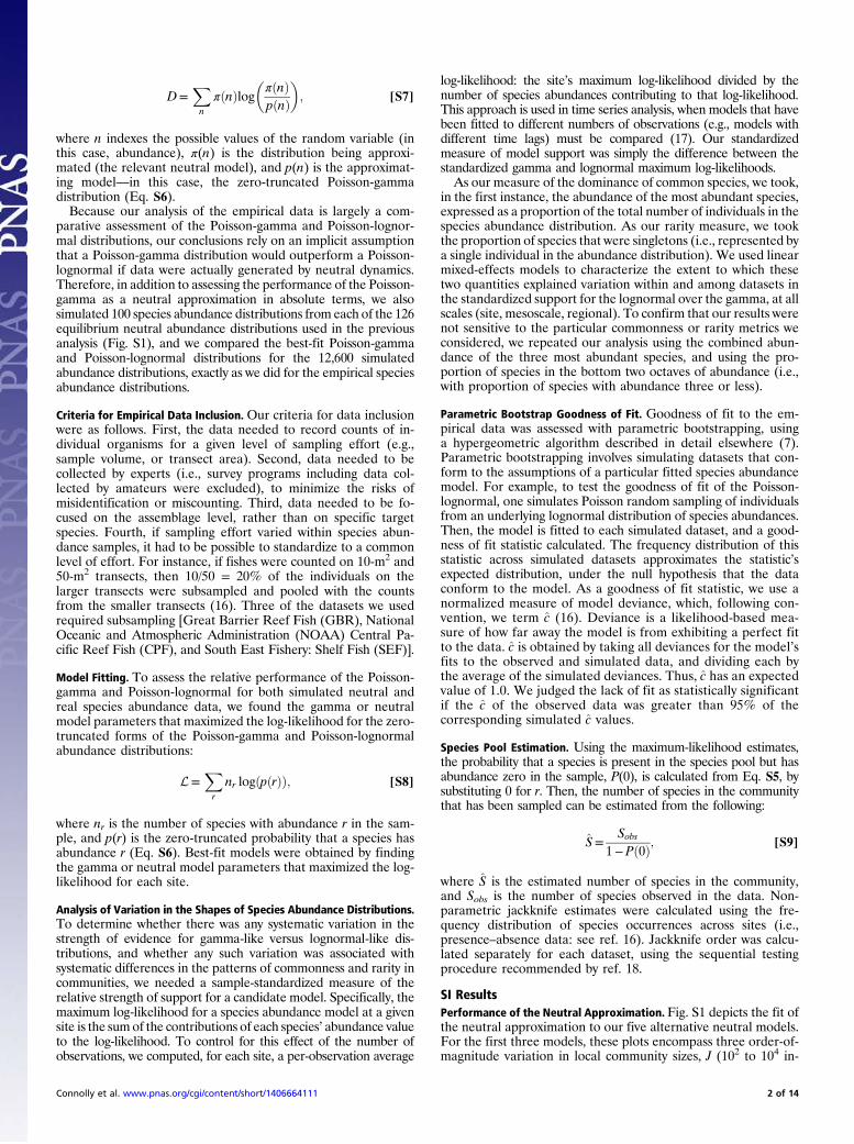
D=Xn

πðnÞlog�πðnÞpðnÞ

�; [S7]

where n indexes the possible values of the random variable (inthis case, abundance), π(n) is the distribution being approxi-mated (the relevant neutral model), and p(n) is the approximat-ing model—in this case, the zero-truncated Poisson-gammadistribution (Eq. S6).Because our analysis of the empirical data is largely a com-

parative assessment of the Poisson-gamma and Poisson-lognor-mal distributions, our conclusions rely on an implicit assumptionthat a Poisson-gamma distribution would outperform a Poisson-lognormal if data were actually generated by neutral dynamics.Therefore, in addition to assessing the performance of the Poisson-gamma as a neutral approximation in absolute terms, we alsosimulated 100 species abundance distributions from each of the 126equilibrium neutral abundance distributions used in the previousanalysis (Fig. S1), and we compared the best-fit Poisson-gammaand Poisson-lognormal distributions for the 12,600 simulatedabundance distributions, exactly as we did for the empirical speciesabundance distributions.

Criteria for Empirical Data Inclusion. Our criteria for data inclusionwere as follows. First, the data needed to record counts of in-dividual organisms for a given level of sampling effort (e.g.,sample volume, or transect area). Second, data needed to becollected by experts (i.e., survey programs including data col-lected by amateurs were excluded), to minimize the risks ofmisidentification or miscounting. Third, data needed to be fo-cused on the assemblage level, rather than on specific targetspecies. Fourth, if sampling effort varied within species abun-dance samples, it had to be possible to standardize to a commonlevel of effort. For instance, if fishes were counted on 10-m2 and50-m2 transects, then 10/50 = 20% of the individuals on thelarger transects were subsampled and pooled with the countsfrom the smaller transects (16). Three of the datasets we usedrequired subsampling [Great Barrier Reef Fish (GBR), NationalOceanic and Atmospheric Administration (NOAA) Central Pa-cific Reef Fish (CPF), and South East Fishery: Shelf Fish (SEF)].

Model Fitting. To assess the relative performance of the Poisson-gamma and Poisson-lognormal for both simulated neutral andreal species abundance data, we found the gamma or neutralmodel parameters that maximized the log-likelihood for the zero-truncated forms of the Poisson-gamma and Poisson-lognormalabundance distributions:

L=Xr

nr logðpðrÞÞ; [S8]

where nr is the number of species with abundance r in the sam-ple, and p(r) is the zero-truncated probability that a species hasabundance r (Eq. S6). Best-fit models were obtained by findingthe gamma or neutral model parameters that maximized the log-likelihood for each site.

Analysis of Variation in the Shapes of Species Abundance Distributions.To determine whether there was any systematic variation in thestrength of evidence for gamma-like versus lognormal-like dis-tributions, and whether any such variation was associated withsystematic differences in the patterns of commonness and rarity incommunities, we needed a sample-standardized measure of therelative strength of support for a candidate model. Specifically, themaximum log-likelihood for a species abundance model at a givensite is the sum of the contributions of each species’ abundance valueto the log-likelihood. To control for this effect of the number ofobservations, we computed, for each site, a per-observation average

log-likelihood: the site’s maximum log-likelihood divided by thenumber of species abundances contributing to that log-likelihood.This approach is used in time series analysis, when models that havebeen fitted to different numbers of observations (e.g., models withdifferent time lags) must be compared (17). Our standardizedmeasure of model support was simply the difference between thestandardized gamma and lognormal maximum log-likelihoods.As our measure of the dominance of common species, we took,

in the first instance, the abundance of the most abundant species,expressed as a proportion of the total number of individuals in thespecies abundance distribution. As our rarity measure, we tookthe proportion of species that were singletons (i.e., represented bya single individual in the abundance distribution). We used linearmixed-effects models to characterize the extent to which thesetwo quantities explained variation within and among datasets inthe standardized support for the lognormal over the gamma, at allscales (site, mesoscale, regional). To confirm that our results werenot sensitive to the particular commonness or rarity metrics weconsidered, we repeated our analysis using the combined abun-dance of the three most abundant species, and using the pro-portion of species in the bottom two octaves of abundance (i.e.,with proportion of species with abundance three or less).

Parametric Bootstrap Goodness of Fit. Goodness of fit to the em-pirical data was assessed with parametric bootstrapping, usinga hypergeometric algorithm described in detail elsewhere (7).Parametric bootstrapping involves simulating datasets that con-form to the assumptions of a particular fitted species abundancemodel. For example, to test the goodness of fit of the Poisson-lognormal, one simulates Poisson random sampling of individualsfrom an underlying lognormal distribution of species abundances.Then, the model is fitted to each simulated dataset, and a good-ness of fit statistic calculated. The frequency distribution of thisstatistic across simulated datasets approximates the statistic’sexpected distribution, under the null hypothesis that the dataconform to the model. As a goodness of fit statistic, we use anormalized measure of model deviance, which, following con-vention, we term c (16). Deviance is a likelihood-based mea-sure of how far away the model is from exhibiting a perfect fitto the data. c is obtained by taking all deviances for the model’sfits to the observed and simulated data, and dividing each bythe average of the simulated deviances. Thus, c has an expectedvalue of 1.0. We judged the lack of fit as statistically significantif the c of the observed data was greater than 95% of thecorresponding simulated c values.

Species Pool Estimation. Using the maximum-likelihood estimates,the probability that a species is present in the species pool but hasabundance zero in the sample, P(0), is calculated from Eq. S5, bysubstituting 0 for r. Then, the number of species in the communitythat has been sampled can be estimated from the following:

S=Sobs

1−Pð0Þ; [S9]

where S is the estimated number of species in the community,and Sobs is the number of species observed in the data. Non-parametric jackknife estimates were calculated using the fre-quency distribution of species occurrences across sites (i.e.,presence–absence data: see ref. 16). Jackknife order was calcu-lated separately for each dataset, using the sequential testingprocedure recommended by ref. 18.

SI ResultsPerformance of the Neutral Approximation. Fig. S1 depicts the fit ofthe neutral approximation to our five alternative neutral models.For the first three models, these plots encompass three order-of-magnitude variation in local community sizes, J (102 to 104 in-

Connolly et al. www.pnas.org/cgi/content/short/1406664111 2 of 14

Page 9

dividuals), because most species abundance distributions are onthe order of hundreds to (occasionally) tens of thousands ofindividuals. Similarly, we show a broad range of immigrationrates from m = 0.01 (1% of newborns are immigrants) to 1.0 (anentirely open local community). We plot a range of values of thebiodiversity parameter, θ, so that the expected number of speciesin the community spanned a very broad range (typically froma low of about five species, for small, isolated communities withlow θ, to many hundreds of species for large, high-immigrationcommunities with large θ). Note that the range of values of θneeded to span these richness values differs between the fissionspeciation model and the first two models, because the param-eter is defined somewhat differently in this model. The pro-tracted speciation model includes an additional parameter, τ′,which is the number of generations required for speciation tooccur, relative to the metacommunity size (the special case τ′ = 0corresponds to the original neutral model). The fourth (in-dependent species) neutral model differs from the others inthat it does not explicitly characterize dynamics at the meta-community scale. Rather, it implicitly assumes that species haveequal abundance in the metacommunity (and thus they all havethe same rate of immigration to the local community, γ), and thatspecies’ local population dynamics are independent of one an-other, and thus a function of only γ and the ratio of local per-capita birth to death rates, x. Because within-species dynamicsare also density independent, this is consistent with the neutralityassumption (individuals have no effect on one another’s per-capita growth rates, regardless of whether they belong to thesame or different species). This density-independent assumptionmeans that the model is a probability distribution of speciesabundances, and not a model of overall species frequencies. Con-sequently, unlike the previous neutral models, it does not predictspecies richness. Similarly, for the spatially explicit model, the formof the species abundance distribution depends on the speciationprobability (ν), and the ratio of the sampling area A (i.e., the localcommunity size) to the squared width of the dispersal kernel, L,rather than either of the latter two variables independently (4).Thus, a given shape for the species abundance distribution cancorrespond to a broad range of different community speciesrichness values, depending on whether A and L are both smallor both large.Fig. S1 shows that the Poisson-gamma neutral approximation

performs very well in the overwhelming majority of cases. Thereare, however, some cases where the approximation performs lesswell. These typically correspond to parameter combinations thatimply very species-poor assemblages. One class of such casescorresponds to small (∼100 individuals), very low-immigration,low-diversity assemblages (∼5 species: e.g., Top Left of Fig. S1A).Here, the neutral model has an elevated probability that onespecies is nearly monodominant (the curve bends upward at theright, for species abundances close to the total community size),which the Poisson-gamma distribution cannot capture. A secondclass of cases, specific to the protracted speciation model, in-volves a flattening of the species abundance distribution at lowabundances (e.g.,m = 0.1, θ = 4, J = 104 in Fig. S1C). This effectis too small to see clearly for the range of parameter valuesshown in Fig. S1, but is somewhat more pronounced in very largecommunities with very low values of the biodiversity parameter(θ ∼ 1), for which the ratio of individuals to species is very high(e.g., a local community with 10,000 individuals but only about10 species). The third class of cases are specific to the fissionspeciation model and involve an excess of rare species, relative tothe Poisson-gamma distribution (e.g., m = 0.01, J = 104, θ = 40 inFig. S1D). As with the second class of cases, this effect is rela-tively small in Fig. S1, but can be more pronounced for verylarge, particularly isolated, communities with few species (e.g.,10,000 individuals and about 10 species, implying mean abun-dances of about 1,000). For the data analyzed in this paper,

however, most sites are very far from these extreme low-diversitycases. The typical (median) site is a sample of 422 individualscontaining 17 species, and very few sites contain so few species atsuch large sample sizes (86% of sites, for instance, have meanspecies abundances of 100 or less). Moreover, the individualdatasets vary substantially in community size and observed spe-cies richness (e.g., mean site richness varies from 9 to 126 speciesacross the 14 datasets, and average species abundances at thesite level range from 4 to 123 across all datasets except one).Thus, the overwhelming majority of our sites could not corre-spond to those regions of parameter space where the Poisson-gamma distribution performs less well as an approximation forneutral dynamics.

Robustness to Ecological and Taxonomic Heterogeneity. Althoughneutral models have previously been applied to very heteroge-neous communities (19), including benthic marine invertebrates(2) [and indeed their capacity to characterize such systems hasbeen invoked as evidence of their robustness (2)], most neutralmodel communities are conceptualized as a guild of organismscompeting for a shared set of resources. Some of our datasets arerelatively taxonomically and ecologically homogeneous [e.g.,Indo-Pacific Coral Crustaceans (IPC), which contains onlycrustaceans associated with dead coral heads]. However, othersare more heterogeneous. Therefore, to determine whether ourresults were sensitive to this taxonomic and ecological hetero-geneity of the assemblages, we classified our species into guilds,where information was available, and reanalyzed our speciesabundance data, limiting the analysis to species from the mostspecies-rich guild for each dataset (Table S3). Such a classifica-tion is necessarily approximate for marine animals, given thehigh degree of omnivory in the ocean. Nevertheless, the analysisallows us to evaluate whether or not our conclusions are sensitiveto the extent of heterogeneity in the data. The resolution of thegroupings for this analysis depended somewhat on both thetaxonomic and ecological heterogeneity of the original data, andalso on the species richness in the samples. Specifically, we usedas a rule of thumb that guilds should have a minimum of 10species, necessitating use of more coarse groupings for morespecies-poor datasets.By restricting the analysis to a subset of the species, the sta-

tistical power to detect differences between Poisson-lognormaland Poisson-gamma species abundances is reduced—the moreheterogeneous the original dataset, the smaller the subset ofspecies that could be included in the analysis. Nevertheless,strong support for the Poisson-lognormal remained: across site,mesoscale, and regional levels, the Poisson-lognormal was strongly(>95%) supported in 27 cases, whereas the Poisson-gamma wasstrongly supported in only 1 (Table S3).

Analysis of Variation in the Shapes of Species Abundance Distributions.Standardizing model support by dividing by the number of ob-served species abundances successfully controlled for the effectsof statistical power shown in Fig. 2, at least at the site level andmesoscale: mixed-effects linearmodel analyses using the number ofdistinct species abundance values as an explanatory variable in-dicated that the overall effect did not differ significantly from zero,and explained about 1–10% of the variation in standardized modelsupport across datasets (see R2 values in Table S4). In contrast,the strength of support for the Poisson-lognormal over the Pois-son-gamma increased strongly with the relative abundance of themost abundant species at site, mesoscale, and regional (whole-dataset) levels. The positive relationship was highly consistentbetween datasets at both the site level and mesoscale (gray lines inFig. S4 A and C), and explained about one-half or more of thevariation (Table S4 and Fig. S4 B, D, and E). In contrast, theproportion of singletons was a poor predictor of relative modelperformance: the estimated direction of the effect was not con-

Connolly et al. www.pnas.org/cgi/content/short/1406664111 3 of 14

Page 10

sistent across datasets at the site level (gray lines in Fig. S5A), andthe estimated overall effect did not differ significantly from zero atany scale (Table S4 and black lines in Fig. S5 A, C, and E) andnever explained more than 16% of the variation (Table S4).To further assess the strength of these results, we repeated our

common-species analysis using the combined relative abundanceof the three most abundant species. This, too, was strongly pos-itively related to support for the Poisson-lognormal distribution(slope: 0.40 ± 0.02, pseudo-R2 = 0.44 at site level; 0.24 ± 0.05,

pseudo-R2 = 0.53 at mesoscale level; 0.15 ± 0.04, R2 = 0.55 atregional scale). Conversely, expanding our definition of rarity toencompass the proportion of species in the bottom two octaves(species with abundance 3 or less) did not improve its effective-ness as a predictor of standardized support for the Poisson-log-normal over the Poisson-gamma: the overall relationship did notdiffer significantly from zero at any scale (no slopes significantlydifferent from zero, pseudo-R2 < 0.02 at site-scale and mesoscalelevels, R2 = 0.21 at regional level).

1. Pueyo S (2006) Diversity: Between neutrality and structure. Oikos 112(2):392–405.2. Hubbell SP (2001) The Unified Neutral Theory of Biodiversity and Biogeography

(Princeton Univ Press, Princeton).3. Volkov I, Banavar JR, Hubbell SP, Maritan A (2007) Patterns of relative species

abundance in rainforests and coral reefs. Nature 450(7166):45–49.4. Rosindell J, Cornell SJ (2013) Universal scaling of species-abundance distributions

across multiple scales. Oikos 122(7):1101–1111.5. Etienne R, Haegeman B (2011) The neutral theory of biodiversity with random fission

speciation. Theor Ecol 4(1):87–109.6. Pielou EC (1977) Mathematical Ecology (Wiley, New York).7. Connolly SR, Dornelas M, Bellwood DR, Hughes TP (2009) Testing species abundance

models: A new bootstrap approach applied to Indo-Pacific coral reefs. Ecology 90(11):3138–3149.

8. Sæther BE, Engen S, Grøtan V (2013) Species diversity and community similarity influctuating environments: Parametric approaches using species abundance distributions.J Anim Ecol 82(4):721–738.

9. Etienne RS, Alonso D (2005) A dispersal-limited sampling theory for species andalleles. Ecol Lett 8(11):1147–1156.

10. Rosindell J, Cornell SJ, Hubbell SP, Etienne RS (2010) Protracted speciation revitalizesthe neutral theory of biodiversity. Ecol Lett 13(6):716–727.

11. He F (2005) Deriving a neutral model of species abundance from fundamentalmechanisms of population dynamics. Funct Ecol 19(1):187–193.

12. Volkov I, Banavar JR, He FL, Hubbell SP, Maritan A (2005) Density dependenceexplains tree species abundance and diversity in tropical forests. Nature 438(7068):658–661.

13. Allen AP, Savage VM (2007) Setting the absolute tempo of biodiversity dynamics. EcolLett 10(7):637–646.

14. Ostling A (2012) Do fitness-equalizing tradeoffs lead to neutral communities? TheorEcol 5(2):181–194.

15. Burnham KP, Anderson DR (2002) Model Selection and Multi-Model Inference: APractical Information-Theoretic Approach (Springer, Heidelberg).

16. Connolly SR, Hughes TP, Bellwood DR, Karlson RH (2005) Community structure ofcorals and reef fishes at multiple scales. Science 309(5739):1363–1365.

17. McQuarrie ADR, Tsai C-L (1998) Regression and Time Series Model Selection (WorldScientific, River Edge, NJ).

18. Burnham KP, Overton WS (1979) Robust estimation of population size when captureprobabilities vary among animals. Ecology 60(5):927–936.

19. de Aguiar MAM, Baranger M, Baptestini EM, Kaufman L, Bar-Yam Y (2009) Globalpatterns of speciation and diversity. Nature 460(7253):384–387.

1 2 5 10 50

1 10−35 10−32 10−21 10−1

E(S) 4

m = 0.01

1 2 5 10 50

E(S) 8

m = 0.1

1 2 5 10 20 50

E(S) 14

m = 1

J 1004

1 2 5 10 50

2 10−31 10−25 10−22 10−1

E(S) 5

1 2 5 10 20

E(S) 17

1 2 5 10

E(S) 36J 100

20

1 2 5 10 50

2 10−31 10−25 10−22 10−1

E(S) 5

1 2 5 10 20

E(S) 23

1 2 3 4 5

E(S) 70J 100

100

1 5 20 100 500

1 10−41 10−31 10−21 10−1

E(S) 11

1 5 20 100 500

E(S) 17

1 5 20 100 500

E(S) 23J 1000

4

1 5 20 100

1 10−41 10−31 10−21 10−1

E(S) 24

1 2 5 20 50

E(S) 53

1 2 5 20 50

E(S) 79J 1000

20

1 2 5 20 100

2 10−41 10−35 10−32 10−21 10−15 10−1

E(S) 39

1 2 5 10 20 50

E(S) 127

1 2 5 10 20

E(S) 240J 1000

100

1 5 50 500 5000

1 10−5

1 10−3

1 10−1

E(S) 20

1 5 50 500 5000

E(S) 26

1 5 50 500 5000

E(S) 32J 10000

4

1 5 50 500

5 10−55 10−45 10−35 10−2

E(S) 64

1 5 50 500

E(S) 98

1 5 50 500

E(S) 125J 10000

20

1 5 20 100 500

1 10−41 10−31 10−21 10−1

E(S) 174

1 2 5 20 100

E(S) 329

1 2 5 20 100

E(S) 462J 10000

100

Species abundance (log scale)

Spe

cies

freq

uenc

y (lo

g sc

ale)

(a) Original neutral model

Fig. S1. (Continued)

Connolly et al. www.pnas.org/cgi/content/short/1406664111 4 of 14

Page 11

1 2 5 10 50

5 × 10−42 × 10−31 × 10−25 × 10−22 × 10−1

E(S) = 3

m = 0.01

1 2 5 10 50

E(S) = 8

m = 0.1

1 2 5 10 20 50

E(S) = 14

m = 1

J = 100θ = 4

1 2 5 10 50

2 × 10−31 × 10−25 × 10−22 × 10−1

E(S) = 5

1 2 5 10 20

E(S) = 17

1 2 5 10

E(S) = 36J = 100θ = 20

1 2 5 10 50

2 × 10−31 × 10−25 × 10−22 × 10−1

E(S) = 5

1 2 5 10 20

E(S) = 23

1 2 3 4 5

E(S) = 70J = 100θ = 100

1 5 20 100 500

5 × 10−55 × 10−45 × 10−35 × 10−2

E(S) = 10

1 5 20 100 500

E(S) = 17

1 5 20 100 500

E(S) = 23J = 1000θ = 4

1 5 20 100

1 × 10−41 × 10−31 × 10−21 × 10−1

E(S) = 24

1 2 5 20 50

E(S) = 53

1 2 5 20 50

E(S) = 79J = 1000θ = 20

1 2 5 20 100

2 × 10−41 × 10−35 × 10−32 × 10−21 × 10−15 × 10−1

E(S) = 39

1 2 5 10 20 50

E(S) = 127

1 2 5 10 20

E(S) = 240J = 1000θ = 100

1 5 50 500 5000

1 × 10−5

1 × 10−3

1 × 10−1

E(S) = 19

1 5 50 500 5000

E(S) = 26

1 5 50 500 5000

E(S) = 32J = 10000θ = 4

1 5 50 500

5 × 10−55 × 10−45 × 10−35 × 10−2

E(S) = 64

1 5 50 500

E(S) = 97

1 5 50 500

E(S) = 125J = 10000θ = 20

1 5 20 100 500

1 × 10−41 × 10−31 × 10−21 × 10−1

E(S) = 173

1 2 5 20 100

E(S) = 328

1 2 5 20 100

E(S) = 462J = 10000θ = 100

Species abundance (log scale)

Spe

cies

freq

uenc

y (lo

g sc

ale)

(b) Protracted speciation model with τ ' = τ Jm = 10−8

1 2 5 10 50

1 × 10−35 × 10−32 × 10−21 × 10−1

E(S) = 3

m = 0.01

1 2 5 10 50

E(S) = 8

m = 0.1

1 2 5 10 20 50

E(S) = 13

m = 1

J = 100θ = 4

1 2 5 10 50

2 × 10−31 × 10−25 × 10−22 × 10−1

E(S) = 5

1 2 5 10 20

E(S) = 17

1 2 5 10

E(S) = 36J = 100θ = 20

1 2 5 10 50

2 × 10−31 × 10−25 × 10−22 × 10−1

E(S) = 5

1 2 5 10 20

E(S) = 23

1 2 3 4 5

E(S) = 69J = 100θ = 100

1 5 20 100 500

5 × 10−55 × 10−45 × 10−35 × 10−2

E(S) = 10

1 5 20 100 500

E(S) = 17

1 5 20 100 500

E(S) = 22J = 1000θ = 4

1 5 20 100

1 × 10−41 × 10−31 × 10−21 × 10−1

E(S) = 24

1 2 5 20 50

E(S) = 52

1 2 5 20 50

E(S) = 77J = 1000θ = 20

1 2 5 20 100

2 × 10−41 × 10−35 × 10−32 × 10−21 × 10−15 × 10−1

E(S) = 38

1 2 5 10 20 50

E(S) = 125

1 2 5 10 20

E(S) = 232J = 1000θ = 100

1 5 50 500 5000

1 × 10−5

1 × 10−3

1 × 10−1

E(S) = 19

1 5 50 500 5000

E(S) = 25

1 5 50 500 5000

E(S) = 29J = 10000θ = 4

1 5 50 500

5 × 10−55 × 10−45 × 10−35 × 10−2

E(S) = 63

1 5 50 500

E(S) = 93

1 5 50 500

E(S) = 111J = 10000θ = 20

1 5 20 100 500

1 × 10−41 × 10−31 × 10−21 × 10−1

E(S) = 170

1 2 5 20 100

E(S) = 306

1 2 5 20 100

E(S) = 394J = 10000θ = 100

Species abundance (log scale)

Spe

cies

freq

uenc

y (lo

g sc

ale)

(c) Protracted speciation model with τ ' = τ Jm = 10−4

Fig. S1. (Continued)

Connolly et al. www.pnas.org/cgi/content/short/1406664111 5 of 14

Page 12

1 2 5 10 50

2 × 10−31 × 10−25 × 10−22 × 10−11 × 100

E(S) = 5

m = 0.01

1 2 5 10 20

E(S) = 16

m = 0.1

1 2 5 10

E(S) = 29

m = 1

J = 100θ = 40

1 2 5 10 50

2 × 10−31 × 10−25 × 10−22 × 10−11 × 100

E(S) = 5

1 2 5 10 20

E(S) = 23

1 2 3 4 5

E(S) = 67

J = 100θ = 200

1 2 5 10 50

2 × 10−31 × 10−25 × 10−22 × 10−11 × 100

E(S) = 5

1 2 5 10 20

E(S) = 25

1.0 1.2 1.4 1.8

E(S) = 91

J = 100θ = 1000

1 5 20 100

2 × 10−41 × 10−35 × 10−32 × 10−21 × 10−1

E(S) = 22

1 2 5 20 50

E(S) = 35

1 2 5 20 50

E(S) = 38

J = 1000θ = 40

1 2 5 20 100

2 × 10−41 × 10−35 × 10−32 × 10−21 × 10−1

E(S) = 38

1 2 5 10 20 50

E(S) = 112

1 2 5 10 20

E(S) = 167

J = 1000θ = 200

1 2 5 20 100

5 × 10−45 × 10−35 × 10−25 × 10−1

E(S) = 45

1 2 5 10 20

E(S) = 204

1 2 3 4 6

E(S) = 500

J = 1000θ = 1000

1 5 50 500

5 × 10−52 × 10−41 × 10−35 × 10−32 × 10−2

E(S) = 37

1 5 50 500

E(S) = 39

1 5 50 500

E(S) = 40

J = 10000θ = 40

1 5 20 100 500

1 × 10−41 × 10−31 × 10−21 × 10−1

E(S) = 140

1 2 5 20 100

E(S) = 186

1 2 5 20 100

E(S) = 196

J = 10000θ = 200

1 2 5 20 100

1 × 10−41 × 10−31 × 10−21 × 10−1

E(S) = 318

1 2 5 10 50

E(S) = 719

1 2 5 10 20 50

E(S) = 909

J = 10000θ = 1000

Species abundance (log scale)

Spe

cies

freq

uenc

y (lo

g sc

ale)

(d) Fission speciation model

1 2 3 4 5

1 × 10−2

5 × 10−2

2 × 10−1

γ = 0.1

1 2 3 4 5 7

γ = 1

1 2 5

γ = 2

x = 0.5

1 2 5 10 20

1 × 10−35 × 10−32 × 10−21 × 10−15 × 10−1

1 2 5 10 20 50 1 2 5 10 20 50

x = 0.9

1 2 5 10 50 200

1 × 10−4

1 × 10−3

1 × 10−2

1 × 10−1

1 2 5 20 50 200 1 2 5 20 100 500

x = 0.99

(e) Independent species model

1 2 5 10 20

2 × 10−3

1 × 10−2

5 × 10−22 × 10−1

ν = 1 × 10−6

1 2 5 10

ν = 1 × 10−4

1 2 5

AL−2 = 4

ν = 1 × 10−2

1 2 5 10 20 50

5 × 10−42 × 10−31 × 10−25 × 10−22 × 10−1

1 2 5 10 20 50 1 2 5 10 20

AL−2 = 16

1 2 5 10 50 200

2 × 10−41 × 10−35 × 10−32 × 10−21 × 10−1

1 2 5 10 50 1 2 5 10 20 50

AL−2 = 64

Species abundance (log scale)

Spe

cies

freq

uenc

y (lo

g sc

ale)

(f) Spatial neutral model

Fig. S1. Examples of the fit of the Poisson-gamma neutral approximation (black line) to the five candidate neutral approximations (blue lines). The fits are shown as“Pueyo plots”: both the vertical and horizontal axes are shown on a log scale. The horizontal axis is truncated at the abundance value where the cumulative expectednumber of species equals 99%of the total (i.e., on average, only 1 of 100 species would be expected to have greater abundance). (A–F) The six different neutral models, asspecified at the top of the corresponding group of panels. For models A–D, E(S) in each panel indicates the expected number of species for that parameter combination.

Connolly et al. www.pnas.org/cgi/content/short/1406664111 6 of 14

Page 13

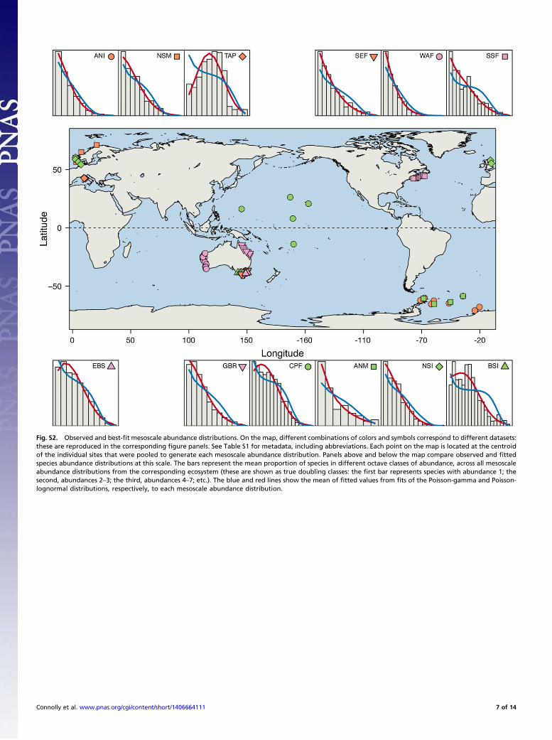
Fig. S2. Observed and best-fit mesoscale abundance distributions. On the map, different combinations of colors and symbols correspond to different datasets:these are reproduced in the corresponding figure panels. See Table S1 for metadata, including abbreviations. Each point on the map is located at the centroidof the individual sites that were pooled to generate each mesoscale abundance distribution. Panels above and below the map compare observed and fittedspecies abundance distributions at this scale. The bars represent the mean proportion of species in different octave classes of abundance, across all mesoscaleabundance distributions from the corresponding ecosystem (these are shown as true doubling classes: the first bar represents species with abundance 1; thesecond, abundances 2–3; the third, abundances 4–7; etc.). The blue and red lines show the mean of fitted values from fits of the Poisson-gamma and Poisson-lognormal distributions, respectively, to each mesoscale abundance distribution.

Connolly et al. www.pnas.org/cgi/content/short/1406664111 7 of 14

Page 14

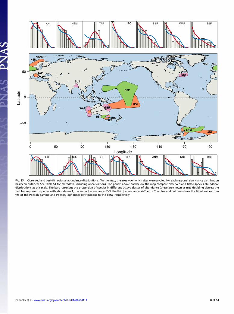
Fig. S3. Observed and best-fit regional abundance distributions. On the map, the area over which sites were pooled for each regional abundance distributionhas been outlined. See Table S1 for metadata, including abbreviations. The panels above and below the map compare observed and fitted species abundancedistributions at this scale. The bars represent the proportion of species in different octave classes of abundance (these are shown as true doubling classes: thefirst bar represents species with abundance 1; the second, abundances 2–3; the third, abundances 4–7; etc.). The blue and red lines show the fitted values fromfits of the Poisson-gamma and Poisson-lognormal distributions to the data, respectively.

Connolly et al. www.pnas.org/cgi/content/short/1406664111 8 of 14

Page 15

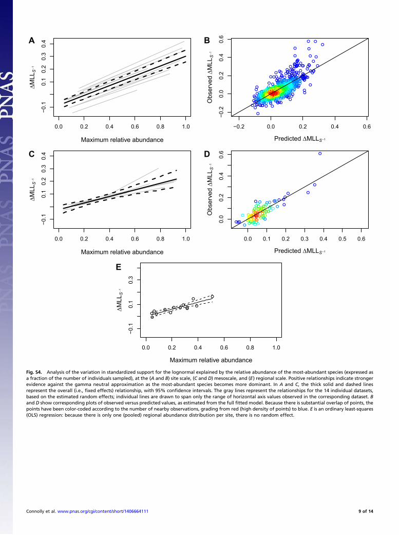
0.0 0.2 0.4 0.6 0.8 1.0

−0.1

0.1

0.2

0.3

0.4

Maximum relative abundance

ΔMLL

S−1

A

−0.2 0.0 0.2 0.4 0.6

−0.2

0.0

0.2

0.4

0.6

Predicted ΔMLLS −1

Obs

erve

d ΔM

LLS

−1

B

0.0 0.2 0.4 0.6 0.8 1.0

−0.1

0.1

0.2

0.3

0.4

Maximum relative abundance

ΔMLL

S−1

C

0.0 0.1 0.2 0.3 0.4 0.5 0.6

0.0

0.2

0.4

0.6

Predicted ΔMLLS −1

Obs

erve

d ΔM

LLS

−1

D

0.0 0.2 0.4 0.6 0.8 1.0

−0.1

0.1

0.3

Maximum relative abundance

Δ MLL

S−1

E

Fig. S4. Analysis of the variation in standardized support for the lognormal explained by the relative abundance of the most-abundant species (expressed asa fraction of the number of individuals sampled), at the (A and B) site scale, (C and D) mesoscale, and (E) regional scale. Positive relationships indicate strongerevidence against the gamma neutral approximation as the most-abundant species becomes more dominant. In A and C, the thick solid and dashed linesrepresent the overall (i.e., fixed effects) relationship, with 95% confidence intervals. The gray lines represent the relationships for the 14 individual datasets,based on the estimated random effects; individual lines are drawn to span only the range of horizontal axis values observed in the corresponding dataset. Band D show corresponding plots of observed versus predicted values, as estimated from the full fitted model. Because there is substantial overlap of points, thepoints have been color-coded according to the number of nearby observations, grading from red (high density of points) to blue. E is an ordinary least-squares(OLS) regression: because there is only one (pooled) regional abundance distribution per site, there is no random effect.

Connolly et al. www.pnas.org/cgi/content/short/1406664111 9 of 14

Page 16

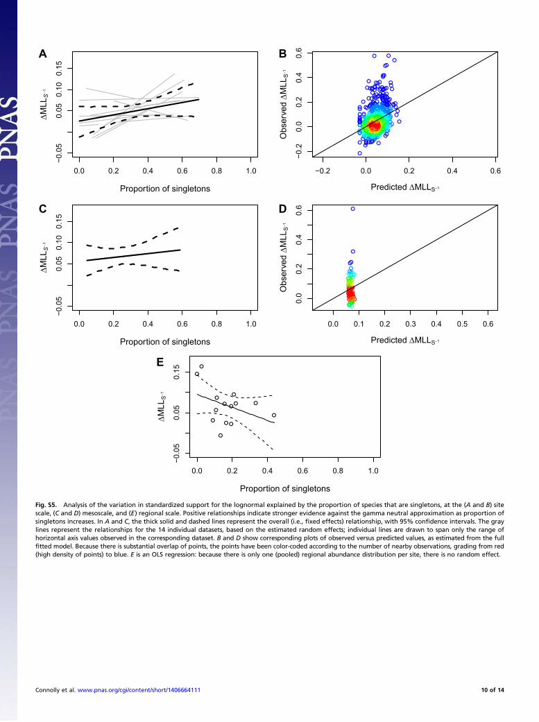
0.0 0.2 0.4 0.6 0.8 1.0

−0.0

50.

050.

100.

15

Proportion of singletons

ΔMLL

S−1

A

−0.2 0.0 0.2 0.4 0.6

−0.2

0.0

0.2

0.4

0.6

Predicted ΔMLLS−1

Obs

erve

d ΔM

LLS−1

B

0.0 0.2 0.4 0.6 0.8 1.0

−0.0

50.

050.

100.

15

Proportion of singletons

ΔMLL

S−1

C

0.0 0.1 0.2 0.3 0.4 0.5 0.6

0.0

0.2

0.4

0.6

Predicted ΔMLLS−1

Obs

erve

d ΔM

LLS−1

D

0.0 0.2 0.4 0.6 0.8 1.0

−0.0

50.

050.

15

Proportion of singletons

ΔMLL

S−1

E

Fig. S5. Analysis of the variation in standardized support for the lognormal explained by the proportion of species that are singletons, at the (A and B) sitescale, (C and D) mesoscale, and (E) regional scale. Positive relationships indicate stronger evidence against the gamma neutral approximation as proportion ofsingletons increases. In A and C, the thick solid and dashed lines represent the overall (i.e., fixed effects) relationship, with 95% confidence intervals. The graylines represent the relationships for the 14 individual datasets, based on the estimated random effects; individual lines are drawn to span only the range ofhorizontal axis values observed in the corresponding dataset. B and D show corresponding plots of observed versus predicted values, as estimated from the fullfitted model. Because there is substantial overlap of points, the points have been color-coded according to the number of nearby observations, grading from red(high density of points) to blue. E is an OLS regression: because there is only one (pooled) regional abundance distribution per site, there is no random effect.

Connolly et al. www.pnas.org/cgi/content/short/1406664111 10 of 14

Page 17

Table S1. Metadata summary of global marine species abundance distribution samples

Dataset name SummaryLatitudinal

limitsLongitudinal

limitsDepth

range, mSamplingmethod Data contact

South East Fishery:Shelf Fish (SEF)

Fish from southeasternAustralia; total of 173species at 189 sites pooledinto 13 mesoscale SADs

−39.0 146.5 16 Fish trawl A.W.−36.4 150.3 254 [email protected]

Western Australia:Deep Fish (WAF)

Fish from western Australia;total of 282 species at 65sites pooled into 23locations

−35.1 111.4 197 Fish trawl A.W.−20.1 115.2 1,580 [email protected]

Great Barrier Reef Fish(GBR)

Fish from underwater visualcensus surveys of coral reefson the Great Barrier Reef(1); total of 195 species at74 sites pooled into 8mesoscale SADs

−23.9 145.3 7 UVS Hugh Sweatman−14.5 152.7 Australian Institute of Marine

Science, Townsville, [email protected]

Antarctic Molluscs(ANM)

Deep-water bivalves from theScotia Arc, Antarctica; totalof 96 species at 20 sitespooled into 4 mesoscaleSADs

−58.2 −60.0 774 Epibenthicsledge

K.L.−65.5 −23.6 6,348 [email protected]

Indo-Pacific CoralCrustaceans (IPC)

Crustacean samplesencompassing a total of411 species from individualdead coral heads at 8 sitesin the Indo-Pacific; notpooled at mesoscale

−23.4 −113.7 10 Handcounts

L.P.6.4 −149.8 [email protected]

Tuscany ArchipelagoFish (TAP)

Fish abundance from theTuscany Archipelago; totalof 39 species at 30 sitespooled into 4 mesoscaleSADs

42.2 9.8 8 UVS L.B.-C.43.1 11.1 12 [email protected]

Eastern Bass StraitInvertebrates (EBS)

Invertebrates from theEastern Bass Strait,Australia (2); total of 801species at 47 sites pooledinto 3 mesoscale SADs

−37.9 148.2 17 Grabsample

R.S.W., G.C.B.P.−37.8 148.7 51 [email protected]

NOAA Central PacificReef Fish (CPF)

Fish from underwater visualsurveys of coral reefsthroughout the Pacific;total of 491 species at 49sites pooled into 5mesoscale SADs

−14.6 −154.8 8.24 UVS R.E.B.28.5 142.8 17.11 [email protected]

SunderbanZooplankton (SUZ)

Zooplankton from Sunderbanmangrove wetland, India;total of 31 species at 7 sites;not pooled at mesoscale

21.6 88.0 2.0 Planktontow

S.K.S.22.3 88.9 8.9 [email protected]

Scotian Shelf Fish (SSF) Fish from the Scotian Shelf,Northwestern Atlantic;total of 98 species at 458sites pooled into 14mesoscale SADs

42.1 −67.2 16 Trawl Steven E. Campana45.6 −57.3 176 Fisheries and Oceans Canada,

Bedford Institute ofOceanography, Dartmouth,[email protected]

Bass Strait IntertidalMacroinvertebrates(BSI)

Invertebrates from the BassStrait, Australia (3); total of98 species at 53 sites pooledinto 5 mesoscale SADs

−39.1 141.4 Intertidal UVS T.D.O.−37.6 149.8 [email protected]

North SeaInvertebrates (NSI)*

Benthic invertebrates fromthe North Sea; total of 244species at 46 sites pooledinto 6 mesoscale SADs

54.3 −1.0 38 vanVeengrab

U.S.60.4 8.0 115 [email protected]

Connolly et al. www.pnas.org/cgi/content/short/1406664111 11 of 14

Page 18

Table S1. Cont.

Dataset name SummaryLatitudinal

limitsLongitudinal

limitsDepth

range, mSamplingmethod Data contact

Norwegian ShelfMacrobenthos(NSM)†

Benthic invertebratescollected along theNorwegian Shelf (4); totalof 805 species at 101 sitespooled into 4 mesoscaleSADs

56.0 1.7 65 vanVeengrab

K.E.E.71.8 23.5 434 [email protected]

Antarctic Isopods(ANI)‡

Isopods from the SouthernOcean (5); total of 502species at 38 sites pooledinto 8 mesoscale SADs

−71.3 0.0 774 Epibenthicsledge

A.B.−58.2 −64.7 6,348 [email protected]

SAD, species abundance distribution; UVS, underwater visual survey (belt transects in all cases).

1. Sweatman H, et al. (2008) Long-Term Monitoring of the Great Barrier Reef (Australian Institute of Marine Science, Townsville, Australia), Status Report no. 8.2. Gray JS, et al. (1997) Coastal and deep-sea benthic diversities compared. Mar Ecol Prog Ser 159:97–103.3. O’Hara TD, Addison PFE, Gazzard R, Costa TL, Pocklington JB (2010) A rapid biodiversity assessment methodology tested on intertidal rocky shores. Aquat Conserv 20(4):452–463.4. Ellingsen KE, Gray JS (2002) Spatial patterns of benthic diversity: Is there a latitudinal gradient along the Norwegian continental shelf? J Anim Ecol 71(3):373–389.5. Brandt A, et al. (2007) First insights into the biodiversity and biogeography of the Southern Ocean deep sea. Nature 447(7142):307–311.

Connolly et al. www.pnas.org/cgi/content/short/1406664111 12 of 14

Page 19

Table

S2.

Summaryoftheab

undan

cedistributionsan

alyz

ed,at

each

ofthethreescales

Dataset

Site

Mesoscale

Reg

ional

N*

S†MRA‡

PS§

N*

S†MRA‡

PS§

N*

S†MRA‡

PS§

Antarctic

Isopods(A

NI)

310(1–2,65

1)40

.2(1–91

)0.24

(0.05–

1.00

)0.49

(0.21–

1.00

)1,47

4(284

–3,53

1)14

1.4(73–

193)

0.13

(0.08–

0.24

)0.36

(0.23–

0.44

)11

,788

502

0.05

0.17

Antarctic

Mollu

scs(A

NM)

109(1–56

0)14

.0(1–33

)0.39

(0.17–

1.00

)0.45

(0.10–

1.00

)54

4(353

–81

6)41

.0(27–

79)

0.34

(0.12–

0.56

)0.37

(0.21–

0.48

)2,17

596

0.21

0.33

Tuscan

yArchipelag

oFish

(TAP)

577(223

–1,11

8)21

.2(16–

26)

0.49

(0.29–

0.74

)0.17

(0.04–

0.33

)4,32

6(3,276

–5,86

7)32

.2(30–

34)

0.50

(0.48–

0.54

)0.08

(0.06–

0.09

)17

,303

390.51

0.03

Indo-Pacific

Coral

Commen

sals

(IPC

)

336(71–

1,01

8)66

.9(25–

127)

0.14

(0.09–

0.20

)0.46

(0.38–

0.62

)NA

NA

NA

NA

644

135

0.06

0.44

SEAustralia

:Sh

elf

Fish

(SEF

)66

0(2–10

,803

)17

.0(1–36

)0.51

(0.16–

1.00

)0.32

(0.00–

0.71

)9,59

8(112

–22

,978

)60

.8(20–

93)

0.37

(0.19–

0.71

)0.24

(0.11–

0.38

)12

4,77

717

30.26

0.16

WAustralia

:Dee

pFish

(WAF)

373(18–

3,71

4)18

.7(8–32

)0.37

(0.07–

0.97

)0.37

(0.09–

0.67

)1,05

5(44–

5,86

8)43

.8(12–

101)

0.37

(0.10–

0.93

)0.35

(0.16–

0.59

)24

,272

282

0.32

0.22

Scotian

Shelf

Fish

(SSF)

855(6–21

,436

)9.4(1–21

)0.65

(0.14–

1.00

)0.28

(0.00–

0.75

)27

,963

(3,493

–78

,019

)37

.5(19–

53)

0.56

(0.33–

0.90

)0.18

(0.05–

0.37

)39

1,48

498

0.32

0.19

EasternBassStrait

Inve

rteb

rates

(EBS)

1,51

9(48–

8,64

1)12

5.7(23–

384)

0.18

(0.05–

0.70

)0.34

(0.00–

0.70

)23

,794

(16,18

2–28

,145

)57

3.7(500

–66

1)0.06

(0.05–

0.07

)0.16

(0.14–

0.18

)71

,382

801

0.05

0.13

Sunderban

Zooplankton

(SUZ)

670(148

–1,19

0)15

.3(7–28

)0.45

(0.24–

0.70

)0.02

(0.00–

0.11

)NA

NA

NA

NA

4,68

931

0.36

0.00

Great

Barrier

Ree

fFish

(GBR)

591(64–

2,53

5)44

.4(7–66

)0.32

(0.08–

0.87

)0.41

(0.14–

0.61

)5,47

1(686

–9,31

5)11

6.9(78–

144)

0.20

(0.14–

0.30

)0.21

(0.14–

0.33

)43

,768

195

0.15

0.11

Cen

tral

Pacific

Ree

fFish

(CPF

)9,67

7(548

–85

,423

)10

4.1(32–

183)

0.30

(0.11–

0.61

)0.20

(0.08–

0.39

)94

,830

(35,81

9–22

3,06

0)23

8.0(171

–29

3)0.30

(0.16–

0.40

)0.13

(0.08–

0.16

)47

4,15

149

10.19

0.09

Norw

egianSh

elf

Macroben

thos

(NSM

)

676(87–

2,67

7)86

.7(35–

148)

0.15

(0.07–

0.51

)0.38

(0.20–

0.63

)17

,074

(5,201

–42

,572

)35

7.5(176

–55

2)0.08

(0.04–

0.11

)0.24

(0.19–

0.29

)68

,298

805

0.08

0.19

NorthSe

aInve

rteb

rates

(NSI)

806(92–

4,60

8)44

.4(28–

77)

0.39

(0.09–

0.87

)0.35

(0.08–

0.51

)6,18

3(1,224

–12

,361

)10

1.2(54–

147)

0.41

(0.10–

0.83

)0.23

(0.09–

0.37

)37

,097

244

0.29

0.21

BassStrait

Intertidal

(BSI)

31,148

(1,200

–11

6,44

4)30

.2(15–

44)

0.61

(0.26–

0.95

)0.14

(0.00–

0.33

)33

0,16

8(96,74

3–64

3,50

0)61

.6(54–

76)

0.47

(0.34–

0.78

)0.07

(0.05–

0.09

)1,65

0,84

298

0.39

0.11

Values

reported

aremea

ns,

withranges

inparen

theses.Dueto

thesm

allnumber

ofsites,

therearenomesoscaleab

undan

cedistributionsforIPCan

dSU

Z(M

aterials

andMethods).Becau

setheregional

abundan

cedistributionpoolsallsamplesin

that

dataset,thereisonly

oneab

undan

cedistribution,so

norangeofva

lues

isreported

.*N

,number

ofindividualssampled.

†S,

number

ofspeciesap

pea

ringin

thesample.

‡MRA,max

imum

relative

abundan

ce(abundan

ceofthemost

abundan

tspecies,as

aproportionofthetotalnumber

ofindividualsin

theab

undan

cedistribution).

§PS

,proportionofspeciessampledthat

aresingletons(i.e.,ab

undan

ce=

1).

Connolly et al. www.pnas.org/cgi/content/short/1406664111 13 of 14

Page 20

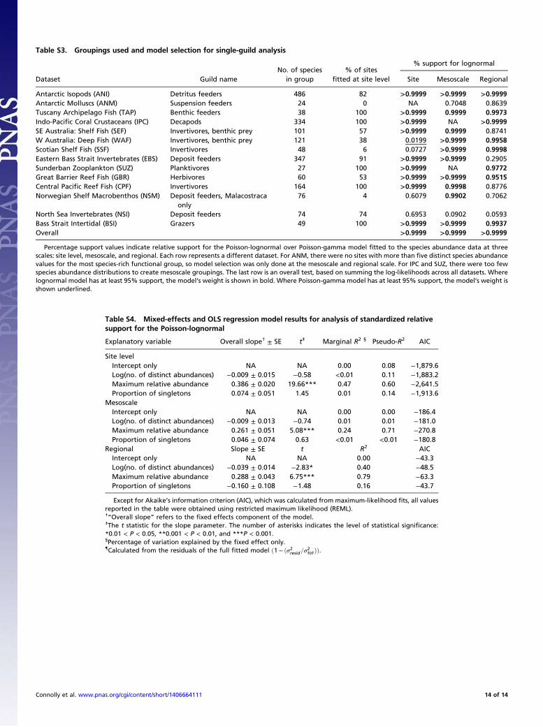
Table S3. Groupings used and model selection for single-guild analysis

Dataset Guild nameNo. of species

in group% of sites

fitted at site level

% support for lognormal

Site Mesoscale Regional

Antarctic Isopods (ANI) Detritus feeders 486 82 >0.9999 >0.9999 >0.9999Antarctic Molluscs (ANM) Suspension feeders 24 0 NA 0.7048 0.8639Tuscany Archipelago Fish (TAP) Benthic feeders 38 100 >0.9999 0.9999 0.9973Indo-Pacific Coral Crustaceans (IPC) Decapods 334 100 >0.9999 NA >0.9999SE Australia: Shelf Fish (SEF) Invertivores, benthic prey 101 57 >0.9999 0.9999 0.8741W Australia: Deep Fish (WAF) Invertivores, benthic prey 121 38 0.0199 >0.9999 0.9958Scotian Shelf Fish (SSF) Invertivores 48 6 0.0727 >0.9999 0.9998Eastern Bass Strait Invertebrates (EBS) Deposit feeders 347 91 >0.9999 >0.9999 0.2905Sunderban Zooplankton (SUZ) Planktivores 27 100 >0.9999 NA 0.9772Great Barrier Reef Fish (GBR) Herbivores 60 53 >0.9999 >0.9999 0.9515Central Pacific Reef Fish (CPF) Invertivores 164 100 >0.9999 0.9998 0.8776Norwegian Shelf Macrobenthos (NSM) Deposit feeders, Malacostraca

only76 4 0.6079 0.9902 0.7062

North Sea Invertebrates (NSI) Deposit feeders 74 74 0.6953 0.0902 0.0593Bass Strait Intertidal (BSI) Grazers 49 100 >0.9999 >0.9999 0.9937Overall >0.9999 >0.9999 >0.9999

Percentage support values indicate relative support for the Poisson-lognormal over Poisson-gamma model fitted to the species abundance data at threescales: site level, mesoscale, and regional. Each row represents a different dataset. For ANM, there were no sites with more than five distinct species abundancevalues for the most species-rich functional group, so model selection was only done at the mesoscale and regional scale. For IPC and SUZ, there were too fewspecies abundance distributions to create mesoscale groupings. The last row is an overall test, based on summing the log-likelihoods across all datasets. Wherelognormal model has at least 95% support, the model’s weight is shown in bold. Where Poisson-gamma model has at least 95% support, the model’s weight isshown underlined.

Table S4. Mixed-effects and OLS regression model results for analysis of standardized relativesupport for the Poisson-lognormal

Explanatory variable Overall slope† ± SE t‡ Marginal R2 § Pseudo-R2 AIC

Site levelIntercept only NA NA 0.00 0.08 −1,879.6Log(no. of distinct abundances) −0.009 ± 0.015 −0.58 <0.01 0.11 −1,883.2Maximum relative abundance 0.386 ± 0.020 19.66*** 0.47 0.60 −2,641.5Proportion of singletons 0.074 ± 0.051 1.45 0.01 0.14 −1,913.6

MesoscaleIntercept only NA NA 0.00 0.00 −186.4Log(no. of distinct abundances) −0.009 ± 0.013 −0.74 0.01 0.01 −181.0Maximum relative abundance 0.261 ± 0.051 5.08*** 0.24 0.71 −270.8Proportion of singletons 0.046 ± 0.074 0.63 <0.01 <0.01 −180.8

Regional Slope ± SE t R2 AICIntercept only NA NA 0.00 −43.3Log(no. of distinct abundances) −0.039 ± 0.014 −2.83* 0.40 −48.5Maximum relative abundance 0.288 ± 0.043 6.75*** 0.79 −63.3Proportion of singletons −0.160 ± 0.108 −1.48 0.16 −43.7

Except for Akaike’s information criterion (AIC), which was calculated from maximum-likelihood fits, all valuesreported in the table were obtained using restricted maximum likelihood (REML).†“Overall slope” refers to the fixed effects component of the model.

‡The t statistic for the slope parameter. The number of asterisks indicates the level of statistical significance:*0.01 < P < 0.05, **0.001 < P < 0.01, and ***P < 0.001.§Percentage of variation explained by the fixed effect only.{Calculated from the residuals of the full fitted model ð1− ðσ2resid=σ2totÞÞ.

Connolly et al. www.pnas.org/cgi/content/short/1406664111 14 of 14