Commonness and rarity of plants in a reserve network: just two faces of the same coin

Commonness and rarity of plants in a reserve network: just twofaces of the same coin

Sara Landi • Alessandro Chiarucci

Received: 20 January 2014 / Accepted: 22 June 2014 / Published online: 17 July 2014

� Accademia Nazionale dei Lincei 2014

Abstract Occurrence of protected and rare species is

regarded as a strong argument for establishing protected

areas and monitoring biodiversity, but while protected

species are clearly identified, some problems exist to define

rare species. It is thus important to know whether common

and unprotected native species are reliable indicators for

protected and rare species. The aims of this paper were to:

(a) analyse the distribution of rarity and commonness of

species, by using different criteria and (b) test if groups of

species with different conservation value (aliens, unpro-

tected natives and protected natives) differ in terms of their

rarity distribution, using the data collected in 604 plots

sampled within 21 protected areas of the central Italy.

Three different criteria were used to classify species as rare

or common. Pearson correlation, least-squares regressions

and Chi-square test were used to compare the species

richness patterns or rare and common species as well as

protected, unprotected native, and alien species. The

number of species classified as common and rare widely

differ according to the adopted criterion. The number of

common and rare species were statistically correlated at

both the plot and protected area scales, even if at the plot

scale the predictive capacity was rather low. Protected

species were significantly rarer than expected, while

unprotected species were significantly more common than

expected; alien species confirmed to be particularly rare in

our study area, with some major alien species being totally

absent in the recorded flora. The richness patterns of

common and rare species defined according to different

criteria have been found to be correlated one to the other,

and both are well related to the richness of protected and

alien species at both the plot and PA scales. Protected

species were better related to common species, while alien

species were better related to rare species. Despite rare

species were numerically more than common species, and

the richness pattern of total species was better predicted by

common species than rare species. Common species con-

firmed to be good indicators of species richness patterns

and also of protected species.

Keywords Alien species � Biodiversity � Common

species � Network � Protected species � Rare species

1 Introduction

Common and rare species have fundamentally different

ecology and understanding how species with different

occurrence contribute to overall patterns of biodiversity

(Jetz et al. 2004; Gaston et al. 2008) is an important

challenge for modern ecology. Many authors reported that

rare species, i.e. those with few individuals or occur-

rences, are the majority in most ecosystems (e.g., Pielou

1969; Gaston 1994, 2011; Lennon et al. 2004; Gaston and

Fuller 2008). Rarity can have different causes and it is

thought to increase the risk of extinction, either through

demographic stochasticity or because of the vulnerability

to environmental changes of species occupying a restric-

ted habitat.

Despite the wide usage of the rarity concept in ecology

and conservation biology, a consistent definition of rarity is

still missing (Rabinowitz et al. 1986; Gaston 1994). Many

measures have been used to define this phenomenon, as the

breadth of geographic range size, degree of habitat

S. Landi (&) � A. Chiarucci

BIOCONNET, BIOdiversity and CONservation NETwork,

Department of Life Sciences, University of Siena, Via P.A.

Mattioli 4, 53100 Siena, Italy

e-mail: [email protected]

123

Rend. Fis. Acc. Lincei (2014) 25:369–380

DOI 10.1007/s12210-014-0313-1

specificity, local frequency, ephemerality, relative abun-

dance, occurrence, and population size (Hartley and Kunin

2003; Gaston 2008). Occurrence of rare and protected plant

species is regarded as a major argument for creating pro-

tected areas and defining their management plans. Some

attempts have also been done to design reserve networks by

using distributional data of selected indicator species

(Hopkinson et al. 2001; Lawler et al. 2003) and this is

likely to be a central theme in future conservation biology.

However, protected species are often chosen on the basis of

‘‘pragmatic’’ issues, such as the presence of one or some

flagship species (Simberloff 1998). While there are no

particular problems in identifying protected species, the

comprehension of which species are rare is still an unre-

solved issue. It is then fundamental to know whether

common and unprotected species are reliable indicator of

rare and protected species, since it is more convenient to

obtain occurrence data for the former than for the latter.

Rarity is a factor that should be taken into account in

conservation biology and, especially, in listing species

which are threatened or need specific management actions

(Hercos et al. 2012). On the other hand, if most species are

rare, it is difficult to include rare species into management

or conservation actions. Moreover, species that are rare in

one locality are not necessarily rare everywhere, because

their abundance may be depressed due to local conditions,

such as unsuitable habitats (Rabinowitz 1981), or even

random processes (Hercos et al. 2012). It is also necessary

to consider that management can have a major role in

controlling commonness and rarity patterns of species.

Therefore, when comparing groups of species with differ-

ent management importance, as it can be the case of alien

and protected species, it is necessary to consider whether

they are common or rare.

Despite common species can be less in number than the

rare species, there is evidence that their contribution to

species richness patterns is often greater than that of rare

species (Jetz and Rahbek 2002; Pearman and Weber 2007;

Mazaris et al. 2008). However, extremely common species

(e.g., those species which occur in all the sampled sites) are

scarcely informative on species richness patterns, since a

species which is present in each sample does not add

nothing to such a pattern or gradient, only uniformly ele-

vates its values of one unit. Nevertheless, analyses of

diversity patterns may be largely based on common rather

rare species, because the latter are swamped by variation

contributed by the former (Lennon et al. 2011). So, a clear

understanding of the contribution of common and rare

species to the richness patterns of groups of species with

different conservation values is fundamental.

The goal of this paper is to analyse the rarity and

commonness patterns of plant species in a regional network

of protected areas, by using an extensive data set on plant

species occurrences (Chiarucci et al. 2012). In particular,

we aim to: (a) analyse the distribution of rarity and com-

monness of species, by using different criteria to define

rarity and (b) test if groups of species with different con-

servation value (alien, native and protected species) differ

in terms of rarity distribution.

2 Methods

Information about the richness of common and rare spe-

cies were obtained from the occurrence data of 1,041

vascular plant species (hereafter referred as S) in 604

plots (each of 100 m2) recorded in 21 protected areas

(PAs) of the province of Siena (central Italy) by using a

stratified random design (Chiarucci et al. 2012). On the

basis of the check-list of alien species of Italy (Celesti-

Grapow et al. 2009) as well as international and regional

laws, each species was classified as: alien (A), unpro-

tected native (N), or protected native (P). The alien spe-

cies group included both archeophyte and neophyte

species, and they can be casual, naturalized or even

invasive (Pysek et al. 2004).

Each species was classified as common (C) or rare

(R) on the basis of three different criteria. In the first two

criteria, the classification of species as common or rare was

based on arbitrary levels of species occurrence: (1) 1 plot

and 1 PA as thresholds and (2) five plots and three PAs as

thresholds. With these criteria, the species recorded with

occurrence level equal or below the threshold levels were

classified as rare, while those with occurrence level above

the threshold were classified as common. Four lists of

common species (CPl1, CPl5 at plot scale, and CPA1,

CPA3 at PA scale) as well as four paired of rare species

(RPl1, RPl5 at plot scale, and RPA1, RPA3 at PA scale)

were obtained. The third criterion (3) used the quartile

method (Gaston 1994) to divide species into common and

rare species: in detail, the 25 % of most frequent species

were classified as common while the remaining 75 % of

species were classified as rare. This criterion resulted in

two lists of common species (CPlq at plot scale and CPAq

at PA scale) and rare species (RPlq at plot scale and RPAq

at PA scale).

Correlation analysis and ordinary linear regressions

were used to detect the existence of relations between pairs

of the species richness variables obtained by the above

classifications. A Chi-squared test was used to test if the

three groups of species with different conservation values

(A, N and P) differed in the distribution of commonness

and rarity, at both the plot and PA scales. The null

hypothesis to be tested is that alien, native, and protected

species do not differ in their patterns of rarity and

commonness.

370 Rend. Fis. Acc. Lincei (2014) 25:369–380

123

The contribution of common and rare species to the

overall richness patterns was assessed using sequential

correlation analysis (e.g., Vazquez and Gaston 2004;

Lennon et al. 2004, 2011; Kreft et al. 2006; Mazaris et al.

2008). For doing this, two rank orders of all the recorded

species (1,041) were built based on species occurrence in

each plot: from the most common to most rare, and from

the more rare to most common. Then, two series of 1,041

sub-assemblages (each made of 604 plots) were built by

sequentially including each species, from the most com-

mon to the most rare and vice versa. In detail, the following

procedure was used to build the series of sub-assemblages

with species ranked in order of commonness: the first sub-

assemblages included only the occurrences of the most

common species (i.e., the species with the highest occur-

rence value) in the 604 plots; then, the second sub-

assemblages were made by adding the second most com-

mon species to the first one. The same procedure was

repeated until all the 1,041 species, from the most common

to the most rare, were added to the sub-assemblages,

reaching a total of 1,041 sub-assemblages. The same pro-

cedure was repeated to build a series of sub-assemblages,

from the most rare to the most common species. Then, the

species richness values of each of the sub-assemblages in

the common to rare (C to R) and rare to common (R to C)

sequences were calculated and correlated with the species

richness of the full assemblages, by using the Pearson’s

product-moment correlation. The same procedure was used

at the PA scale (1,041 sub-assemblages, each of 21 PAs,

for both the C to R and R to C sequences). This resulted in

two series of correlation coefficients (one for the C to R

sequence and one for the R to C sequence), for both the

plot and PA scale. Then, these two sequences of correlation

coefficients were plotted against the number of species

included into the sub-assemblages. This allowed to

understand how the species richness of the full-assem-

blages can be predicted by the species richness values of

the sub-assemblages of the n most common or the n most

rare species.

Then, a frequency index that weighs each species

according to its occurrence at plot and PA scale was

computed. The proportion of plots and PAs occupied by a

given species (p) was used to calculate the index p(1-p).

This index represents a measure of the spatial information

provided by each species (Lennon et al. 2004), with species

with intermediate occurrence providing more information

than extremely rare or extremely common ones. The index

p(1-p) was compared across the different groups of spe-

cies (A, N, and P, as well as common and rare species), to

compare the information contribution they provide. The

existence of statistically significant differences between the

p(1-p) index between common and rare species, at both

plot (ICPl1 vs. IRPl1, ICPl5 vs. IRPl5, and ICPlq vs.

IRPlq) and PA scale (ICPA1 vs. IRPA1, ICPA3 vs. IRPA3,

and ICPAq vs. IRPAq) were tested by the Mann–Whitney

test for independent samples. The non parametric Kruskal–

Wallis test was adopted to test for statistically significant

differences in the p(1-p) index among the three groups of

species with different conservation interest (A, N, and P).

All analyses were performed with R version 3.0.2 (R Core

Team 2013), in particular ‘‘vegan’’ package (Oksanen et al.

2013).

3 Results

None of the species was recorded in all the sampled plots,

nor in all the PAs. The species with the highest frequency

at the plot scale was Hedera helix (298 plots, 49.3 % of the

total), and the species with the highest frequency at the PA

scale were Hedera helix, Quercus cerris, and Brachypo-

dium rupestre (19 PAs, 90.5 % of the total). The species

classified as protected were 95, being 9.1 % of the total

richness (mean per plot = 1.3; mean per PA = 12.0),

while 48 species were classified as alien (4.6 %; mean per

plot = 0.5; mean per PA = 6.2) and 898 as unprotected

natives (86.3 %; mean per plot = 29.7; mean per

PA = 208.2).

The classification of species common and rare showed

markedly different results, according to the different

adopted criteria (Table 1), with the number of species

classified as common, at the plot and PA scales, decreasing

from the first to the third approach.

The number of common species classified as protected

was significantly lower than expected, whereas the number

of rare species classified as protected was significantly

higher than expected (Table 2). This pattern was observed

at the both plot and PA scales, for the two first

Table 1 Number of species classified as common (CPl1, CPl5, CPlq)

or rare (RPl1, RPl5, RPlq) at plot scale, and as common (CPA1,

CPA3, CPAq) or rare (RPA1, RPA3, RPAq) at PA scale, according to

the three different criteria used

Pl1 Pl5 Plq

CPl1 RPl1 CPl5 RPl5 CPlq RPlq

Mean 31.1 0.4 29.6 1.9 25.4 6.1

Range 0–118 0–6 0–107 0–15 0–90 0–33

Tot 808 233 511 530 267 774

PA1 PA3 PAq

CPA1 RPA1 CPA3 RPA3 CPAq RPAq

Mean 212.1 14.3 181.9 44.5 131.4 95.0

Range 23–526 0–45 17–419 1–151 8–258 2–312

Tot 741 300 484 557 267 774

Rend. Fis. Acc. Lincei (2014) 25:369–380 371

123

classification criteria. The results of the quartile criterion

were slightly different and showed that, at both the plot and

PA scales, both the number of alien and protected species

classified as common were significantly less than expected

(Table 2).

The species richness values of rare species were statis-

tically related to those of common species, at both the plot

and PA scales (Fig. 1), even if at the plot scale the pre-

dictive capacity was rather low (Fig. 1, upper panels). At

the plot scale (Fig. 1), the capacity to predict the number of

rare species by using the number of common species

increased from the more restrictive criterion to the less

restrictive ones. A much higher predictive capacity is

observed at the PA scale for all the different adopted cri-

teria (Fig. 1). Given the autocorrelated nature of the data

(total species richness is made by summing rare and

common species), the number of common and rare species

were also significant predictors of total species richness, at

both plot and PA scales.

The richness of protected species was statistically

predictable by using the richness of rare and protected

species (Fig. 2). At the plot scale, the predictive capacity

of protected species by rare species was rather low, while

it was higher using common species. At the PA scale the

predictive capacity of protected species by common and

rare species was similar and much higher, but the

covariance in species-area relationships certainly con-

tributed to this.

Table 2 Chi-square test, showing the observed values of alien (A),

protected native (P) and unprotected native (N) species classified as

common (CPl1, CPl5, CPlq) or rare (RPl1, RPl5, RPlq) at plot scale,

and as common (CPA1, CPA3, CPAq) or rare (RPA1, RPA3, RPAq)

at PA scale

Pl1 Pl5 Plq

CPl1 RPl1 CPl5 RPl5 CPlq RPlq

A 27 21 10 38 4 ; 44

P 40 ; 55 : 25 ; 70 : 9 ; 86

N 726 172 476 422 254 644

v2 = 86.97 v2 = 40.56 v2 = 23.85

PA1 PA3 PAq

CPA1 RPA1 CPA3 RPA3 CPAq RPAq

A 24 24 11 37 5 ; 43

P 45 ; 50 : 22 ; 73 : 10 ; 85

N 672 226 451 447 252 646

v2 = 42.60 v2 = 36.54 v2 = 19.98

The bold values indicate statistically significant values, and if the

observed number is significantly higher (:) or lower (;) than expected

Fig. 1 Regression graphs showing the predictive power of rare

species (RPl1, RPl5, RPlq, RPA1, RPA3, RPAq) by common species

(CPl1, CPl5, CPlq, CPA1, CPA3, CPAq), according to the different

criteria used for defining rare species (see ‘‘Methods’’ for details), at

both the plot (Pl) and the PA scales. Pl1: RPl1 = 0.02 CPl1-0.160,

R2 = 0.16; Pl5: RPl5 = 0.07 CPl5-0.23, R2 = 0.26; Plq:

RPlq = 0.27 CPlq-0.79, R2 = 0.432; PA 1: RPA1 = 0.09 CPA1-

3.99, R2 = 0.787; PR3: RPA3 = 0.34 CPA3-17.12, R2 = 0.847;

PAq: RPAq = 1.07 CPAq-45.88, R2 = 0.843. All values were

statistically significant p \ 0.001

372 Rend. Fis. Acc. Lincei (2014) 25:369–380

123

The richness of alien species was statistically predict-

able by using the richness of rare and protected species

(Fig. 3), but with a different pattern than protected species.

Contrary to the protected species, the richness of alien

species was better predicted by rare species than by com-

mon species at the plot scale. At the PA scale, the

Fig. 2 Regression graphs showing (in the first and third lines) the

predictive power of protected species (P) by rare species (RPl1, RPl5,

RPlq, RPA1, RPA3, RPAq), according to the different criteria used for

defining rare species (see ‘‘Methods’’ for details), at both the plot and the

PA scales. Pl1: P = 0.33 RPl1 ? 0.14, R2 = 0.037; Pl5: P = 0.13

RPl5 ? 1.01, R2 = 0.059; Plq: P = 0.08 RPlq ? 0.77, R2 = 0.124;

PA1: P = 0.66 RPA1 ? 2.62, R2 = 0.875; PA3: P = 0.21

RPA3 ? 2.57, R2 = 0.852; PAq: P = 0.10 RPAq ? 2.02, R2 =

0.848. All values were statistically significant p \ 0.001. Regression

graphs showing (in the second and fourth lines) the predictive power of

protected species (P) by common species (CPl1,CPl5, CPlq, CPA1,

CPA3, CPAq), according to the different criteria used for defining

common species (see ‘‘Methods’’ for details), at both the plot and the PA

scales. Pl1: P = 0.04 CPl1 ? 0.12, R2 = 0.250; Pl5: P = 0.04

CPl5 ? 0.10, R2 = 0.255; Plq: P = 0.05 CPlq ? 0.04, R2 = 0.259;

PA1: P = 0.06 CPA1-1.42, R2 = 0.862; PA3: P = 0.08 CPA3-

2.17, R2 = 0.852; PAq: P = 0.12 CPAq-4.01, R2 = 0.838. All values

were statistically significant p \ 0.001

Rend. Fis. Acc. Lincei (2014) 25:369–380 373

123

Fig. 3 Regression graphs showing (in the first and third lines) the

predictive power of alien species (A) by rare species (RPl1, RPl5,

RPlq, RPA1, RPA3, RPAq), according to the different criteria used

for defining rare species (see ‘‘Methods’’ for details), at both the plot

(Pl) and the PA scales. Pl1: A = 0.35 RPl1 ? 0.38, R2 = 0.112; Pl5:

A = 0.1366 RPl5 ? 0.25, R2 = 0.159; Plq: A = 0.18 RPlq ? 0.05,

R2 = 0.146; PA1: A = 0.39 RPA1 ? 0.69, R2 = 0.715; PA3:

A = 0.14 RPA3 ? 0.17, R2 = 0.826, PAq: A = 0.07 RPAq-0.25,

R2 = 0.839. Regression graphs showing (in the second and fourth

lines) the predictive power of alien species (A) by common species

(CPl1,CPl5, CPlq, CPA1, CPA3, CPAq), according to the different

criteria used for defining common species (see ‘‘Methods’’ for

details), at both the plot (Pl) and the PA scales. Pl1:

A = 0.01 CPl1 ? 0.19, R2 = 0.051; Pl5: A = 0.01 CPl5 ? 0.23,

R2 = 0.039; Plq: A = 0.01 CPlq ? 0.29, R2 = 0.022; PA1:

A = 0.04 CPA1-2.12, R2 = 0.781; PA3: A = 0.05 CPA3-2.42,

R2 = 0.743; PAq: A = 0.07 CPAq-0.25, R2 = 0.839. All values

were statistically significant p \ 0.001

374 Rend. Fis. Acc. Lincei (2014) 25:369–380

123

predictive capacity of alien species by common and rare

species at PA scale was similar and much higher, but even

in this case the covariance in the species-area relationships

certainly contributed to this.

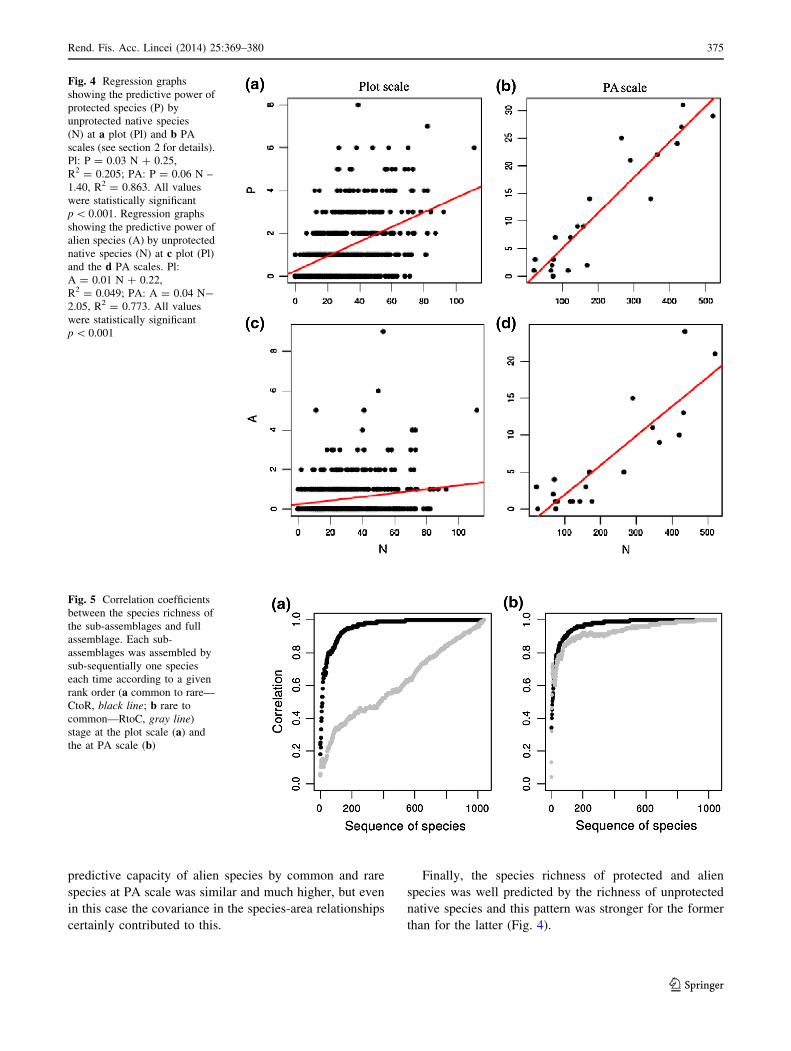
Finally, the species richness of protected and alien

species was well predicted by the richness of unprotected

native species and this pattern was stronger for the former

than for the latter (Fig. 4).

Fig. 4 Regression graphs

showing the predictive power of

protected species (P) by

unprotected native species

(N) at a plot (Pl) and b PA

scales (see section 2 for details).

Pl: P = 0.03 N ? 0.25,

R2 = 0.205; PA: P = 0.06 N –

1.40, R2 = 0.863. All values

were statistically significant

p \ 0.001. Regression graphs

showing the predictive power of

alien species (A) by unprotected

native species (N) at c plot (Pl)

and the d PA scales. Pl:

A = 0.01 N ? 0.22,

R2 = 0.049; PA: A = 0.04 N-

2.05, R2 = 0.773. All values

were statistically significant

p \ 0.001

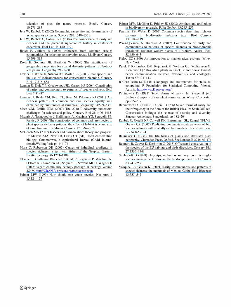
Fig. 5 Correlation coefficients

between the species richness of

the sub-assemblages and full

assemblage. Each sub-

assemblages was assembled by

sub-sequentially one species

each time according to a given

rank order (a common to rare—

CtoR, black line; b rare to

common—RtoC, gray line)

stage at the plot scale (a) and

the at PA scale (b)

Rend. Fis. Acc. Lincei (2014) 25:369–380 375

123

The correlation coefficients between the species richness

of each of the sub-assemblages and the species richness of

the full assemblages increased with different patterns along

the C to R and R to C sequences (Fig. 5). Common species

contributed more to species richness patterns than rare

species, creating most of spatial structure in richness pat-

terns. At the plot scale, the correlation coefficients for the C

to R sequence were much higher than those achieved in the

R to C sequence (Fig. 5a). Thus, common species gave a

much closer approximation to the overall species richness

patterns than rare species; only 6.3 % of common species

were needed in the C to R to achieve a correlation coeffi-

cient of 0.8 (p \ 0.001, Fig. 5a), and 11.2 % to reach a

correlation coefficient of 0.9 (p \ 0.001, Fig. 5a). On the

other hand, the correlation coefficient of R to C sequence

increased slowly following an almost linear curve and it

was necessary to include 71.6 % of rare species into the

sub-assemblages to achieve a correlation coefficient of 0.8

(p \ 0.001, Fig. 5a), and 85.5 % to reach a correlation

coefficient of 0.9 (p \ 0.001, Fig. 5a). A less clear

difference between the C to R and sequences was observed

at the PA scale: 4.3 and 8.4 % of the common species were

required to reach correlation coefficient of 0.8 (p \ 0.001,

Fig. 5b) and 0.9 (p \ 0.001, Fig. 5b) in C to R sequence,

while 6.8 and 17.6 % of rare species were needed to

achieve correlation coefficient of 0.8 (p \ 0.001, Fig. 5b)

and 0.9 (p \ 0.001, Fig. 5b) in the R to C sequence.

Common and rare species differed in the values of the

information content about variability of species richness, as

shown by the values of the p(1-p) index (Fig. 6). The non

parametric Mann–Whitney test revealed statistically signifi-

cant differences between common and rare species at both the

plot scale and PA scale (df = 1; p \ 0.001). Even the groups

of species with different conservation values (A, N, and P)

provided statistically significant different values of the

information content p(1-p) (Fig. 7). In particular, the Krus-

kal–Wallis test revealed statistically significant differences at

both the plot scale and at PA scale (df = 2, p \ 0.001), with

the unprotected native species having higher values of the

index than protected and alien species (Fig. 7).

Fig. 6 Box-plot of values of the p(1-p) index between common and rare species at both plot (ICPl,1 IRPl1, ICPl5, IRPl5, ICPlq, IRPlq) and PA

scale (ICPA1, IRPA1, ICPA3, IRPA3, ICPAq, IRPAq)

376 Rend. Fis. Acc. Lincei (2014) 25:369–380

123

4 Discussion

4.1 Commonness and rarity

A growing evidence suggests that common rather than rare

species shape the overall distribution patterns of species

richness (Vazquez and Gaston 2004; Gaston and Fuller

2007; Gaston 2008; Perez-Quesada and Brazeiro 2012).

This is not intuitive, since local and regional assemblages

are normally composed by numerous rare species and few

common ones (Colwell and Coddington 1994; Gotelli and

Colwell 2001). Despite some differences in the operational

division of species into common and rare, according to

their occurrences into the plots or protected areas, this

study showed that a very high proportion of species are rare

but the common ones are most responsible for richness

patterns, as already reported by other studies (Jiguet and

Julliard 2006; Pearman and Weber 2007). This study also

confirmed the rule that in a regional survey most of the

recorded species are rare and few are common (Pielou

1969; Gaston 1994): this pattern is known as the ‘‘Law of

infrequency’’ (Raunkiaer 1934; Palmer 1995) and it has

negative implications for biodiversity surveying and

recording, since any of such programs will inevitably miss

rare species (Gaston 1994; Chiarucci et al. 2011). The

recording of rare species also depend on the adopted

sampling approach, as well as on the abundance or

occurrence data which are collected (Gotelli and Colwell

2001). Specific sampling designs for recording rare species

are almost impossible, for both practical and biological

reasons (Elzinga et al. 2001). So, rare species can only be

defined as those with abundance or occurrence values

below arbitrary thresholds in a given sample or data col-

lection. There are also additional caveats which affect

rarity measures in observational studies, as those repre-

sented by bias in sampling design (Chiarucci 2007) and

statistical artefacts (Palmer et al. 2008).

Biologists frequently lump various groups of species

under the term rare, partly because a consistent vocabulary

for the types of rarity is still missing, or not globally

accepted, and this may obscure important features of a

diverse group (Rabinowitz et al. 1986; Gaston 1994). In

addition to definition arguments, it is really difficult to

recognise common and rare species even because changes

in the rarity thresholds affect the definition of rare species

and the relationships they are involved. This is also con-

firmed by the present findings, which demonstrated

important changes in grouping rare species on the basis of

the adopted criteria. Despite the division of species into

common and rare is dependent on the selected criterion,

almost all data sets are intrinsically incomplete and they

are certainly more biased for rare species than for common

species (Guisan et al. 2006; Kreft et al. 2006; Diekmann

et al. 2007; Chiarucci et al. 2008; Hedgren and Weslien

2008). This makes inference on rare species more difficult

than that on common species.

Fig. 7 Box-plot of values of the

p(1-p) index between alien,

native, and protected species at

both plot (IPlA, IPlN, IPlP) and

PA scale (IPAA, IPAN, IPAP)

Rend. Fis. Acc. Lincei (2014) 25:369–380 377

123

Since common species contribute more than rare species

to the species richness patterns, their occurrence is a good

proxy for biodiversity and this can be used because com-

mon species are easier to record than rare species. Com-

mon species can also be used as important indicators of the

overall habitat quality, since they often constitute struc-

turally important components of habitats (McGeoch 2007).

From a practical point of view, focusing the survey on

common and easily recognized species could improve the

understanding of species richness patterns, and their

determinants, with relatively low costs (Vazquez and

Gaston 2004). The greater contribution of common species

to the patterns of species richness can profitably be used to

investigate where common species are absent, rather than

where rare species are present, to determine patterns of

species richness on the basis of easily detectable species

(Lennon et al. 2004). In addition, richness of common

species is well correlated to environmental variables, as it

was reported for birds in South Africa (Jetz and Rahbek

2002) and Britain (Evans et al. 2005), tropical fishes (Mora

and Robertson 2005), neotropical palms (Kreft et al. 2006)

and birds in South America (Rahbek et al. 2007). Given the

relatively large amount of information available for com-

mon species (e.g., life-history and physiological traits),

explanations for the richness patterns may be more pre-

cisely sought than have hitherto been possible.

In this and other studies (e.g., Lennon et al. 2004;

Mazaris et al. 2008), the information contents provided by

the common species were higher than that provided by the

rare species, since the former gave a closer approximation

to overall patterns of species richness than the latter. Then,

given that the richness of common species results to be

more correlated with overall species richness and more

informative, common species could be considered as better

indicators of that overall richness. Pearman and Weber

(2007), using data on butterflies, birds, and vascular plants,

confirmed that sampling common species alone can well

describe the spatial patterns of total species richness. This

is apparently contrary to the long-prevailing assumptions

that rare species would make better indicators (Gaston

2008).

This study also confirmed the importance of the scale in

controlling the patterns of commonness and rarity. At small

grain, as the plot scale, the relations between the richness

of common and rare species are significant but often with

low predictive value. On the other hand, at larger grains, as

it was the case of the PA scale, the relationships are much

higher. The covariance due to the species–area relation-

ships is likely to be the determinant of the relations

observed at larger scale in this study (see Chiarucci et al.

2012 for an analysis on the same data set).

In summary, it is suggested that common species can be

used as adequate indicators of biodiversity patterns, at

various scales, allowing better understanding of the deter-

minants of species richness patterns. This study showed

that, despite the intensity of relationship changes at plot

and PA scale, the general pattern does not change. Mazaris

et al. (2008) stated that this pattern is independent of the

size of sampling unit. Then, the richness of common spe-

cies can be considered the best predictor of overall species

richness at different spatial scales.

4.2 Protected and alien species

Often the focus of conservation planning and biodiversity

monitoring is limited to groups of species with special

features or management interest, as in the case of protected

(e.g., Regnery et al. 2013; Hochkirch et al. 2013) or alien

(e.g., Mace and Baillie 2007) species. Protected and alien

species are highly heterogeneous groups and can include

species with various degrees of rarity, in dependence of

different mechanisms controlling their distribution and

abundance. The richness patterns of common and rare

species defined according to different criteria have been

found to be correlated one to the other, and both well

related to the richness of protected and alien species.

However, protected and alien species showed different

patterns: the richness of protected species was better rela-

ted to the richness of common species while the richness of

alien species was better related to the richness of rare

species. This is a peculiar pattern, despite some potential

links to the sampling design adopted for collecting the data.

The probabilistic design adopted in this study is certainly

more suited for recording the occurrence of common rather

than rare species. A stratified sampling is an objective,

well-defined, and easy method, free from personal bias

(Chiarucci 2007), and it is suitable in long-term monitoring

programs and for statistical analysis, but it is not effective

for recording those species which have strict habitat

requirement, small range size or population density

(Diekmann et al. 2007), as it can be the case for protected

or alien species.

In fact, both rare and alien species revealed to be rarer

than the unprotected native, and this makes more difficult

to collect good data about their abundance or distribution

and this is likely to be a major limitation for management

and monitoring purposes.

Regarding protected species, the results of this study

suggest that higher the richness of common species higher

is the richness of protected species, confirming the

importance of protecting sites with high species richness

and using common species as the best currency for biodi-

versity estimates. Common species largely determine the

species richness patterns and these are also reflected by the

patterns of protected species richness. The coincidence

between common and protected species can be a sampling

378 Rend. Fis. Acc. Lincei (2014) 25:369–380

123

artefact (Diekmann et al. 2008; Palmer et al. 2008) due to

differences in sampling design and intensity. However,

while the relation and the larger scale (whole protected

area) could be biased because of the covariance in species–

area relationships, the relation at the plot scale is certainly

worth of understanding since this was a well standardised

sampling.

Alien species are group made by a variety of different

species, with extremely different strategies and abundance

patterns; they can be invasive and colonize most of the

habitats, thus being really common, or limited to a few

places where they have been introduced. Species as

Robinia pseudoacacia, Arundo donax, and Ailanthus

altissima are considered to be the major invasive neophyte

species in Tuscany (Arrigoni and Viegi 2011), but they

were almost absent in the data recorded by this survey.

Robinia pseudoacacia is invasive neophyte and has been

recorded in 8 PAs and 17 plots, confirming its abundance.

On the other hand, Arundo donax and Ailanthus altissima

have not been recorded in the present survey, confirming

the low level of alien invasion of this area but also the

low probability of including such alien species in a

probabilistic data collection. Thus, alien species are con-

firmed to be rare in this area, as it was indicated by the

results of the p(1-p) index but also by the lack of some

major alien species in the recorded data. The scarce level

of alien species occurrence is easy to understand for this

specific data, given their focus on a network of protected

areas, which are relatively well preserved (Chiarucci et al.

2012).

Alien species usually occupy more nutrient-rich, human-

modified habitats, and show tighter habitat similarity as a

group, compared with the more variable native species

(Dawson et al. 2011). The difference in the level of habitat

similarity within alien and native species groups may

reflect introduction sources and habitat disturbance events

(Chrobock et al. 2011). Different results, with potentially

many common alien species, could have been found in

more disturbed areas, but there is no much data available

on the distribution of rarity among alien species in com-

parison to native species.

Acknowledgments We thank everyone who contributed to data

collection within the MoBiSIC project, the University of Siena and

the Province of Siena for their support. Moreover, we would like to

thank the Editor and two anonymous referees for valuable comments

and suggestions on a previpus version of the manuscript.

References

Arrigoni PV, Viegi L (2011) La flora vascolare esotica spontaneizzata

della Toscana. Regione Toscana, Firenze

Celesti-Grapow L, Alessandrini A, Arrigoni PV, Banfi E, Bernardo L,

Bovio M, Brundu G, Cagiotti MR, Camarda I, Carli E, Conti F,

Fascetti S, Galasso G, Gubellini L, La Valva V, Lucchese F,

Marchiori S, Mazzola P, Peccenini S, Poldini L, Pretto F, Prosser

F, Siniscalco C, Villani MC, Viegi L, Wilhalm T, Blasi C (2009)

Inventory of the non-native flora of Italy. Plant Biosyst

143:386–430

Chiarucci A (2007) To sample or not to sample? That is the question

for the vegetation scientist. Folia Geobot 42:209–216

Chiarucci A, Bacaro G, Rocchini D (2008) Quantifying plant species

diversity in a Natura 2000 network: old ideas and new proposals.

Biol Conserv 141:2608–2618

Chiarucci A, Bacaro G, Scheiner SM (2011) Old and new challenges

in using species diversity for assessing biodiversity. Phil Trans R

Soc B 366:2426–2437

Chiarucci A, Bacaro G, Filibeck G, Landi S, Maccherini S, Scoppola

A (2012) Scale dependence of plant species richness in a

network of protected areas. Biodivers Conserv 21:503–516

Chrobock T, Kempel A, Fischer M, Kleunen M (2011) Introduction

bias: cultivated alien plant species germinate faster and more

abundantly than native species in Switzerland. Basic Appl Ecol

12:244–250

Colwell RK, Coddington JA (1994) Estimating terrestrial biodiversity

through extrapolation. Philos Tran R Soc London B 345:101–118

Dawson W, Fischer M, Kleunen M (2011) The maximum relative

growth rate of common UK plant species is positively associated

with their global invasiveness. Global Ecol Biogeogr 20:299–306

Diekmann M, Kuhne A, Isermann M (2007) Random vs non-random

sampling: effects on species abundance, species richness and

vegetation-environment relationships. Folia Geobot 42:179–190

Diekmann M, Dupre C, Kolb A, Metzing D (2008) Forest vascular plants

as indicators of plant species richness: a data analysis of a flora atlas

from northwestern Germany. Plant Biosyst 142:584–593

Elzinga CL, Salzer DW, Willoughby JW, Gibbs JP (2001) Monitoring

plant and animal population. Blackwell Science, Malden

Evans KL, Greenwood JJD, Gaston KJ (2005) Relative contribution

of abundant and rare species to species–energy relationships.

Biol Lett 1:87–90

Gaston KJ (1994) Rarity. Chapman Hall, London

Gaston KJ (2008) Biodiversity and extinction: the importance of

being common. Prog Phys Geogr 32:73–79

Gaston KJ (2011) Common ecology. Bioscience 61:354–362

Gaston KJ, Fuller RA (2007) Biodiversity and extinction: losing the

common and the widespread. Prog Phys Geogr 31:213–225

Gaston KJ, Fuller RA (2008) Commonness, population depletion and

conservation biology. Trends Ecol Evol 23:14–19

Gaston KJ, Chown SL, Evans KL (2008) Ecogeographical rules:

elements of a synthesis. J Biogeogr 35:483–500

Gotelli NJ, Colwell RK (2001) Quantifying biodiversity: procedures

and pitfalls in the measurement and comparison of species

richness. Ecol Lett 4:379–391

Guisan A, Broennimann O, Engler R, Vust M, Yoccoz NG, Lehmann

A, Zimmermann NE (2006) Using niche-based models to

improve the sampling of rare species. Conserv Biol 20:501–511

Hartley S, Kunin WE (2003) Scale dependency of rarity, extinction

risk and conservation priority. Conserv Biol 17:1559–1570

Hedgren O, Weslien J (2008) Detecting rare species with random or

subjective sampling: a case study of red-listed saproxylic beetles

in Boreal Sweden. Conserv Biol 22:212–215

Hercos AP, Sobansky M, Queiroz HL, Magurran AE (2012) Local

and regional rarity in a diverse tropical fish assemblage. Proc R

Soc B 280:2012–2076

Hochkirch A, Schmitt T, Beninde J, Hiery M, Kinitz T, Kirschey J,

Matenaar D, Rohde K, Stoefen A, Wagner N, Zink A, Lotters S,

Veith M, Proelss A (2013) Europe needs a new vision for a

Natura 2020 network. Conserv Lett 6:462–467

Hopkinson P, Travis JMJ, Evans J, Gregory R, Telfer MG, Williams

PH (2001) Flexibility and the use of indicator taxa in the

Rend. Fis. Acc. Lincei (2014) 25:369–380 379

123

selection of sites for nature reserves. Biodiv Conserv

10:271–285

Jetz W, Rahbek C (2002) Geographic range size and determinants of

avian species richness. Science 297:1548–1551

Jetz W, Rahbek C, Colwell RK (2004) The coincidence of rarity and

richness and the potential signature of history in centers of

endemism. Ecol Lett 7:1180–1191

Jiguet F, Julliard R (2006) Inferences from common species

communities for selecting conservation areas. Biodivers Conserv

15:799–815

Kreft H, Sommer JH, Barthlott W (2006) The significance of

geographic range size for spatial diversity patterns in Neotrop-

ical palms. Ecography 29:21–30

Lawler JJ, White D, Sifneos JC, Master LL (2003) Rare species and

the use of indicatorgroups for conservation planning. Conserv

Biol 17:875–882

Lennon JJ, Koleff P, Greenwood JJD, Gaston KJ (2004) Contribution

of rarity and commonness to patterns of species richness. Ecol

Lett 7:81–87

Lennon JJ, Beale CM, Reid CL, Kent M, Pakeman RJ (2011) Are

richness patterns of common and rare species equally well

explained by environmental variables? Ecography 34:529–539

Mace GM, Baillie JEM (2007) The 2010 Biodiversity indicators:

challenges for science and policy. Conserv Biol 21:1406–1413

Mazaris A, Tzanopoulos J, Kallimanis A, Matsinos YG, Sgardelis SP,

Pantis JD (2008) The contribution of common and rare species to

plant species richness patterns: the effect of habitat type and size

of sampling unit. Biodivers Conserv 17:3567–3577

McGeoch MA (2007) Insects and bioindication: theory and progress.

In: Stewart AJA, New TR, Lewis OT (eds) Insect conservation

biology, Commonwealth Agricultural Bureau (CABI Interna-

tional).Wallingford: pp 144–74

Mora C, Robertson DR (2005) Causes of latitudinal gradients in

species richness: a test with fishes of the Tropical Eastern

Pacific. Ecology 86:1771–1782

Oksanen J, Guillaume Blanchet F, Kindt R, Legendre P, Minchin PR,

O’Hara RB, Simpson GL, Solymos P, Stevens MHH, Wagner H

(2013) vegan: community ecology package. R package version

2.0–9. http://CRAN.R-project.org/package=vegan

Palmer MW (1995) How should one count species. Nat Area J

15:124–135

Palmer MW, McGlinn D, Fridley JD (2008) Artifacts and artifictions

in biodiversity research. Folia Geobot 43:245–257

Pearman PB, Weber D (2007) Common species determine richness

patterns in biodiversity indicator taxa. Biol Conserv

138:109–119

Perez-Quesada A, Brazeiro A (2012) Contribution of rarity and

commonness to patterns of species richness in biogeographic

transitions regions: woody plants of Uruguay. Austral Ecol

38:639–645

Pielou EC (1969) An introduction to mathematical ecology. Wiley,

New York

Pysek P, Richardson DM, Rejmanek M, Webster GL, Williamson M,

Kirschner J (2004) Alien plants in checklist and floras: towards

better communication between taxonomists and ecologists.

Taxon 53:131–143

R Core Team (2013) R: a language and environment for statistical

computing. R Foundation for Statistical Computing, Vienna,

Austria. http://www.R-project.org/

Rabinowitz D (1981) Seven forms of rarity. In: Synge H (ed)

Biological aspects of rare plant conservation. Wiley, Chichester,

pp 205–217

Rabinowitz D, Cairns S, Dillon T (1986) Seven forms of rarity and

their frequency in the flora of the British Isles. In: Soule ME (ed)

Conservation biology: the science of scarcity and diversity.

Sinauer Associates, Sunderland, pp 182–204

Rahbek C, Gotelli NJ, Colwell RK, Entsminger GL, Rangel TFLVB,

Graves GR (2007) Predicting continental-scale patterns of bird

species richness with spatially explicit models. Proc R Soc Lond

B 274:165–174

Raunkiaer C (1934) The life forms of plants and statistical plant

geography. Clarendon Press, Oxford. Soc London B 274:165–174

Regnery B, Couvet D, Kerbiriou C (2013) Offsets and conservation of

the species of the EU habitats and birds directives. Conserv Biol

27:1335–1343

Simberloff D (1998) Flagships, umbrellas and keystones: is single-

species management passe in the landscape era? Biol Conserv

83:247–257

Vazquez LB, Gaston KJ (2004) Rarity, commonness, and patterns of

species richness: the mammals of Mexico. Global Ecol Biogeogr

13:535–542

380 Rend. Fis. Acc. Lincei (2014) 25:369–380

123