i A FEASIBILITY STUDY INTO THE POSSIBILITY OF IONOSPHERIC PROPAGATION OF LOW VHF (30 ~ 35 MHZ) SIGNALS BETWEEN SOUTH AFRICA AND CENTRAL AFRICA A thesis submitted in fulfilment of the requirements for the degree of MASTER of SCIENCE of Rhodes University by Petrus Johannes Coetzee November 2009

Welcome message from author
This document is posted to help you gain knowledge. Please leave a comment to let me know what you think about it! Share it to your friends and learn new things together.
Transcript

8/4/2019 Coetzee MSc Thesis
http://slidepdf.com/reader/full/coetzee-msc-thesis 1/73
i
A FEASIBILITY STUDY INTO THE POSSIBILITY OF
IONOSPHERIC PROPAGATION OF LOW VHF (30 ~
35 MHZ) SIGNALS BETWEEN SOUTH AFRICA AND
CENTRAL AFRICA
A thesis submitted in fulfilment of the requirements for the degree of
MASTER of SCIENCE
of
Rhodes University
by
Petrus Johannes Coetzee
November 2009

8/4/2019 Coetzee MSc Thesis
http://slidepdf.com/reader/full/coetzee-msc-thesis 2/73
ii
Abstract
The role of the South African National Defence Force (SANDF) has changed considerably in the last
decade. The emphasis has moved from protecting the country's borders to peacekeeping duties in
Central Africa and even further North. Communications between the peacekeeping missions and the
military bases back in South Africa is vital to ensure the success of these missions.
Currently use is made of satellite as well as High Frequency (HF) communications. There are
drawbacks associated with these technologies (high cost and low data rates/interference respectively).
Successful long distance ionospheric propagation in the low Very High Frequency (VHF) range will
complement the existing infrastructure and enhance the success rate of these missions.
This thesis presents a feasibility study to determine under what ionospheric conditions such low VHF
communications will be possible. The International Reference Ionosphere (IRI) was used to generate
ionospheric data for the reflection point(s) of the signal. The peak height of the ionospheric F2 layer
(h m F 2 ) was used to calculate the required antenna elevation angle. Once the elevation angle is known
it is possible to calculate the required F2 layer critical frequency (f o F 2 ). The required f o F 2 value was
calculated by assuming a Maximum Useable Frequency (MUF) of 20% higher than the planned
operational frequency.
It was determined that single hop propagation is possible during the daytime if the smoothed sunspot
number (SSN) exceeds 15. The most challenging requirement for successful single hop propagation is
the need of an antenna height of 23 m. For rapid deployment and semi-mobile operations within a
jungle environment it may prove to be a formidable obstacle.

8/4/2019 Coetzee MSc Thesis
http://slidepdf.com/reader/full/coetzee-msc-thesis 3/73
iii
Acknowledgement
I wish to extend my sincere gratitude and high appreciation to my supervisor Dr. Lee-Anne McKinnell
for her guidance towards the success of this study.
Thanks to my wife, Gillian, and sons Jean-Pierre and Jayden for their continuous support.
And most important of all: to the Creator of the heavens and the Earth, and the ionosphere, how great
Thou are!

8/4/2019 Coetzee MSc Thesis
http://slidepdf.com/reader/full/coetzee-msc-thesis 4/73
iv
Table of Contents
Abbreviations.................................................................................................................x
Chapter 1. Introduction..................................................................................................1
1.1 Introduction and overview................................................................................1
1.2 Problem statement...........................................................................................1
1.3 Propagation prediction programs.....................................................................2
1.4 Defining a sample communication path...........................................................2
1.5 Single hop reflection point position..................................................................3
1.6 Double Hop Propagation..................................................................................4
1.7 Determining the possibility of long distance sky wave propagation of VHF
signals ........................................................................................................................5
1.8 Overview ..........................................................................................................6
Chapter 2. Principles of Ionospheric Communications.................................................7
2.1 Introduction ......................................................................................................7
2.2 The ionosphere ................................................................................................7
2.3 Characterising the ionosphere.......................................................................11
2.4 HF radio propagation .....................................................................................14
2.5 Summary........................................................................................................19
Chapter 3 - Advantages of the 30 - 35 MHz Band (Compared to HF)........................20
3.1 Introduction ....................................................................................................20
3.2 Low probability of intercept ............................................................................20
3.3 Low received noise ........................................................................................21
3.4 Reduced interference from lightning discharges ...........................................22
3.5 Small antennas ..............................................................................................23
3.6 High data rates...............................................................................................24
3.6 Summary........................................................................................................25
Chapter 4 - Possible Single Hop Propagation Investigation.......................................26

8/4/2019 Coetzee MSc Thesis
http://slidepdf.com/reader/full/coetzee-msc-thesis 5/73
v
4.1 Introduction ....................................................................................................26
4.2 F2-layer peak height (hmF2) requirements ...................................................26
4.3 Elevation angles for single hop propagation..................................................28
4.4.1 Required elevation angles assuming a flat Earth ..................................29
4.4.2 Required elevation angles for a curved Earth........................................30
4.5 Required antenna height................................................................................30
4.6 Summary........................................................................................................32
Chapter 5 - Possible Double Hop Propagation Investigation......................................33
5.1 Introduction ....................................................................................................33
5.2 Most Northerly reflection point .......................................................................34
5.3 Most Southerly reflection point ......................................................................35
5.4 Required elevation angles assuming a curved Earth ....................................37
5.5 Required critical frequency (foF2) for double hop propagation .....................38
5.6 Summary........................................................................................................40
Chapter 6 - Sample Communication Solution.............................................................41
6.1 Introduction ....................................................................................................41
6.2 Required critical frequency (foF2) for single hop communications................41
6.3 Skip or dead zone..........................................................................................43
6.4 Propagation via the E layer............................................................................44
6.5 Antenna and transmitter power requirements ...............................................45
6.5.1 Undesired high angle radiation .................................................................46
6.5.2 Antenna polarisation .................................................................................47
6.5.3 Path loss....................................................................................................48
6.5.4 Expected Received Power Level ..............................................................49
6.5.5 Expected Received Signal-to-Noise Ratio................................................50
6.6 Validation of results........................................................................................51
6.7 Summary........................................................................................................55

8/4/2019 Coetzee MSc Thesis
http://slidepdf.com/reader/full/coetzee-msc-thesis 6/73
vi
Chapter 7 – Conclusion and Discussion .....................................................................57
7.1 Conclusion .....................................................................................................57
7.2 Future work ....................................................................................................58
Appendixes..................................................................................................................59
Appendix A: South African Aircraft Modelling Association’s (SAAMA)
frequencies...............................................................................................................59
Appendix B: Derivation of propagation-distance formula [Elwell, 1982].........60
References ..................................................................................................................62

8/4/2019 Coetzee MSc Thesis
http://slidepdf.com/reader/full/coetzee-msc-thesis 7/73
vii
List of Figures
Figure 1.1: Simplified single hop propagation scenario ................................................3 Figure 1.2: Simplified double hop propagation scenario...............................................5 Figure 2.1: Sample daytime electron density profile of the ionosphere as modelled by
the IRI ............................................................................................................................8 Figure 2.2: Sample night-time electron density profile as modelled by the IRI ............9 Figure 2.3: The ionosphere in terms of critical frequencies as modelled by the IRI ...10 Figure 2.4: (Vertical incidence) Ionogram as generated by the Grahamstown
ionosonde....................................................................................................................12 Figure 2.5: Simplified geometrical propagation model................................................14 Figure 2.6: Calculated propagation of a 5 MHz signal through the ionosphere .........17 Figure 2.7: Calculated propagation of an 11.5 MHz signal through the ionosphere ..18 Figure 3.1: Received noise (from RECOMMENDATION ITU-R P.372-8, Radio noise,
2003) ...........................................................................................................................22 Figure 3.2: Worldwide lightning probability distribution (from Christian et al, 2003)...23 Figure 4.1: IRI generated winter 24 hour peak layer height profile for SSN > 60 at the
reflection point (single hop scenario) ..........................................................................27 Figure 4.2: IRI generated summer 24 hour peak layer height profile for SSN > 60 at
the reflection point (single hop scenario) ....................................................................28 Figure 4.3: Simplified geometrical propagation model assuming a flat earth.............29 Figure 4.4: 32 MHz horizontal dipole 23 m above ground ..........................................31 Figure 5.1: Simplified double hop scenario.................................................................33 Figure 5.2: IRI generated winter 24 hour peak layer height profile for SSN > 60 at the
most northerly reflection point (double hop scenario).................................................34

8/4/2019 Coetzee MSc Thesis
http://slidepdf.com/reader/full/coetzee-msc-thesis 8/73
viii
Figure 5.3: IRI generated summer 24 hour peak layer height profile for SSN > 60 at
the most northerly reflection point (double hop scenario)...........................................35 Figure 5.4: IRI generated winter 24 hour peak layer height profile for SSN > 60 at the
most southerly reflection point (double hop scenario) ................................................36 Figure 5.5: IRI generated summer 24 hour peak layer height profile for SSN > 60 at
the most Southerly reflection point (double hop scenario)..........................................37 Figure 5.6: IRI generated winter f o F 2 for all SSN at the most Southerly reflection point
(double hop scenario)..................................................................................................39 Figure 5.7: IRI generated summer f o F 2 for all SSN at the most Southerly reflection
point (double hop scenario).........................................................................................40 Figure 6.1: IRI generated winter f o F 2 for all SSN at the reflection point (single hop
scenario)......................................................................................................................42 Figure 6.2: IRI generated winter f o F 2 for an SSN > 15 at the reflection point (single
hop scenario)...............................................................................................................43 Figure 6.3: IRI generated winter f o E for an SSN > 100 at the reflection point (single
hop scenario)...............................................................................................................44 Figure 6.4: Basic half-wave dipole antenna................................................................45 Figure 6.5: Unwanted, high angle radiation of a single dipole 23 m above ground
level .............................................................................................................................46 Figure 6.6: Radiation pattern of two horizontal dipoles at 18 and 23 m fed in phase.47 Figure 6.7: Radiation pattern of a quarter-wave vertical antenna 5 m above ground
level .............................................................................................................................48 Figure 6.8: Ray tracing results between Pretoria and Kisangani for a SSN of 15 at
12h00 UT.....................................................................................................................51 Figure 6.9: Ray tracing results between Pretoria and Kisangani for a SSN of 100 at
08h00 UT.....................................................................................................................53

8/4/2019 Coetzee MSc Thesis
http://slidepdf.com/reader/full/coetzee-msc-thesis 9/73
ix
Figure 6.10: Ray tracing elevation angle results between Pretoria and Kisangani for a
SSN of 15 at 10h00 UT ...............................................................................................54 Figure 6.11: Ray tracing elevation angle results between Pretoria and Kisangani for a
SSN of 100 at 10h00 UT .............................................................................................55 Figure B.1: Geometry for derivation of propagation-distance formula for a curved
Earth ............................................................................................................................60

8/4/2019 Coetzee MSc Thesis
http://slidepdf.com/reader/full/coetzee-msc-thesis 10/73
x
Abbreviations
Abbreviation Meaning
λ Wavelength in metre
ARTIST Automatic Real Time Ionospheric Scaling Technique
c Speed of light in metres per secondCAT Central African Time (GMT + 2 hours)
dB Decibel
dBi Gain in Decibel referenced to an isotropic antenna
dBm Decibel referenced to 1 mWatt
DRC Democratic Republic of the Congo
E East
EFOT Estimated Frequency Optimum de Travail (80 ~ 85% of the FOT)
E-M Electro-Magnetic (wave)
EUV Extreme Ultraviolet
F Operating frequency
fb Gyro-frequency
FM Frequency Modulationf o E Critical or plasma frequency of the E layer (for the Ordinary-ray)
f o F 1 Critical or plasma frequency of the F1 layer (for the Ordinary-ray)
f o F 2 Critical or plasma frequency of the F2 layer (for the Ordinary-ray)
f x F 2 Critical or plasma frequency of the F2 layer (for the Extra-ordinary-ray)
FOT Frequency Optimum de Travail or Frequency for Optimum Traffic
GMT Greenwich Mean Time
HF High Frequency (3 to 30 MHz)
h m F 2 Height of the F2 layer at the critical frequency
Hz Hertz
ICASA Independent Communications Authority of South Africa
IRI(-R) International Reference Ionosphere (-Recommendation)
ITU International Telecommunications Union
kHz kilohertz (1 000 Hz)
km kilometre
m metre
MHz Megahertz (1 000 000 Hz)
MUF Maximum Useable Frequency
N North
NVIS Near Vertical Incidence Signal(s)
OFDM Orthogonal Frequency Division Multiplexing
O-ray Ordinary ray of a signal that travelled through the ionosphere
OWF Optimum Working FrequencyP Pagina (Page)
PIM Parameterized Ionospheric Model
QAM Quadrature Amplitude Modulation
RF Radio Frequency
RSA Republic of South Africa
RX Receiver
S South

8/4/2019 Coetzee MSc Thesis
http://slidepdf.com/reader/full/coetzee-msc-thesis 11/73
xi
SAAMA South African Aircraft Modelling Association
SANDF South African National Defence Force
SNR Signal-to-Noise Ratio
SSB Single Side Band modulation
SSN Smoothed Sunspot Number
TX Transmitter
UT Universal (Coordinated) Time
VHF Very High Frequency (30 - 300 MHz)W Watts
X-ray Extraordinary ray of a signal that travelled through the ionosphere

8/4/2019 Coetzee MSc Thesis
http://slidepdf.com/reader/full/coetzee-msc-thesis 12/73
1
Chapter 1. Introduction
1.1 Introduction and overview
The role of the South African National Defence Force (SANDF) has changed considerably in the last
decade. The emphasis has moved from protecting the country's borders to peacekeeping duties in
Central Africa and even further North (Coetzee, 2004). Communications between the peacekeeping
missions and the military bases back in the Republic of South Africa (RSA) are vital to the success of
these missions. Currently use is made of microwave satellite communications as well as High
Frequency (HF) Radio Communications (3 – 30 MHz).
Satellite communications are expensive, especially if high volumes of data need to be sent. HF is
reliable but suffers from bandwidth restrictions and interference. Unlawful elements may also relatively
easily intercept the HF transmissions using freely available equipment.
Long distance sky wave communications utilising the low end of the Very High Frequency (VHF) band
just above the classic HF frequency range may go a long way to minimise the drawbacks of classic HF
communications and supplement the existing communications infrastructure of the SANDF.
1.2 Problem statement
In the absence of easily available frequency prediction programs this thesis describes the use of first
principles to determine the possibility of low, VHF (30 ~ 35 MHz) propagation between the Republic of
South Africa and Central Africa. The ionospheric conditions under which such propagation may be
possible will be determined. The types, polarization and heights of suitable antennas as well as the
transmitter output power, receiver sensitivity and the expected received Signal-to-Noise Ratio will be
investigated and calculated.

8/4/2019 Coetzee MSc Thesis
http://slidepdf.com/reader/full/coetzee-msc-thesis 13/73
Chapter 1. Introduction and Overview
2
1.3 Propagation prediction programs
Long distance HF communications are possible due to the reflection and refraction of signals by the
ionosphere (Davies, 1990). The ionosphere is an extremely dynamic medium that is mostly influenced
by solar activity. Ionospheric models are used to describe and predict the behaviour of the ionosphere
and also to provide the data required for the analysis and prediction of ionospheric propagation.
Ray-tracing techniques are used to model the propagation of an electro-magnetic (E-M) wave through
the ionosphere. It is thus possible to determine if a specified frequency propagates between two given
positions at a certain time and date. This technique is widely used in frequency prediction programs
that are, in the information age, freely available on the Internet.
Unfortunately currently none of these freely available programs can perform point-to-point predictions
for frequencies above 30 MHz, the upper limit of the classic HF band. Above 30 MHz these programs
revert to ground refraction techniques and line-of-sight propagation principles. These techniques are
totally unsuitable for the requirements of long distance, ionospheric sky wave propagation.
1.4 Defining a sample communication path
The typical locations of the stations must be defined in order to determine the most likely ionospheric
reflection point of the signal. The locations of the possible reflection point(s) are required to enable
accurate ionospheric data to be obtained for the analysis of a possible low VHF communications link.
For this study the possibility of single hop and double hop propagation was investigated. Any point in
Central Africa or the Republic of South Africa could have been chosen for the study but the following
two were considered the most appropriate:

8/4/2019 Coetzee MSc Thesis
http://slidepdf.com/reader/full/coetzee-msc-thesis 14/73
Chapter 1. Introduction and Overview
3
Kisangani, a city in the Democratic Republic of the Congo (DRC) was chosen as a representative
Central African location. It is very near to the equator and nearly due North from South Africa's main
cities. It is also relatively close to Uganda, Burundi and other “hot spots” in Central Africa. Due to the
nature of HF communications the results of this study will thus be representative for the majority of the
Central African region. The geographic latitude and longitude of Kisangani is 0.25° North and 25.12°
East.
Pretoria (25.45° South, 28.10° East) was chosen as the other end of the communications link. Pretoria
is the capital city of South Africa and home to various military headquarters and bases. The majority of
communications between Central African peace keeping forces and the Republic of South Africa will
thus originate or terminate in Pretoria.
1.5 Single hop reflection point position
The great circle distance between Kisangani and Pretoria is 2 927 km. The most probable reflection
point for single hop propagation is the halfway point between Kisangani and Pretoria namely 12.85°
South and 26.61° East. The great circle distance to the reflection point is thus 1 463 km. The possible
single hop propagation scenario is depicted in Figure 1.1. For illustrative purposes use is made of a
flat earth and a flat ionosphere. In Chapter 4 the differences in required radiation angles for a flat earth
and a curved earth for the sample propagation path are highlighted.
Figure 1.1: Simplified single hop propagation scenario
Kisangani,DRC
(0.25° N,
25.12° E)
Ionosphere
Earth
Pretoria,RSA
(25.45° S,
28.10° E)
Signal Path
ReflectionPoint
(12.85° S,
26.61° E)
1 464 km

8/4/2019 Coetzee MSc Thesis
http://slidepdf.com/reader/full/coetzee-msc-thesis 15/73
Chapter 1. Introduction and Overview
4
1.6 Double Hop Propagation
To investigate the possibility of double hop propagation between Kisangani and Pretoria, it is assumed
that the signal will be reflected at a quarter of the great circle distance from the transmitter to the
receiver. This translates to reflection points at 6.18° South, 25.87° East and at 19.03° South, 27.36°
East. The great circle distance from the transmitter/receiver to the reflection point is thus 732 km. The
possible double hop propagation scenario is depicted in Figure 1.2. For illustrative purposes use is
made of a flat earth and a flat ionosphere.

8/4/2019 Coetzee MSc Thesis
http://slidepdf.com/reader/full/coetzee-msc-thesis 16/73
Chapter 1. Introduction and Overview
5
Figure 1.2: Simplified double hop propagation scenario
1.7 Determining the possibility of long distance sky wave propagation of
VHF signals
The ionospheric peak parameters (F2-layer critical frequency, f o F 2 , and height, h m F 2 ) for the reflection
point(s) of the signal are supplied by a model of the ionosphere, in this case the International
Reference Ionosphere (IRI)(Bilitza, 2000). Maximum Useable Frequency (MUF) calculations are then
utilised with the aid of the peak layer parameters to determine under what ionospheric conditions the
propagation of low VHF signals will be possible.
The required elevation angles for the layer heights are also calculated. From this the required height of
the antenna is determined with the aid of an antenna simulation program. The expected path loss and
received signal-to-noise ratio is calculated for when propagation may be possible.
Kisangani
(0.25° N,
25.12° E)
Ionosphere
Earth
Pretoria
(25.45° S,
28.10° E)
Signal Path
ReflectionPoint 1
(6.18° S,
25.87° E)
ReflectionPoint 2
(19.03° S,
27.36° E)
1 464 km

8/4/2019 Coetzee MSc Thesis
http://slidepdf.com/reader/full/coetzee-msc-thesis 17/73
Chapter 1. Introduction and Overview
6
1.8 Overview
This thesis consists of seven chapters.
In Chapter 1 the background for this study is given. The problem is stated as well as sample positions
for the transmitting and receiving stations and the refraction points for possible single and double hop
propagation. The limitations of currently freely available software tools are noted and a method is
proposed to solve the problem from first principles.
Chapter 2 describes the principles of ionospheric propagation. Applicable terms such as MUF, f o F 2 , as
well as the "tools of the trade" including ionosondes and ionograms, the composition of the ionosphere
and ray-tracing is discussed.
Chapter 3 discusses the advantages of the low VHF band (30 ~ 35 MHz) over the classic HF band (3 -
30 MHz) for the type of communications required by the SANDF. Antenna sizes, atmospheric noise,
lightning distribution, probability of intercept, achievable data tempos, etc are some of the topics that
give this frequency range an edge over the HF band, if propagation is possible.
In Chapter 4 the possibility of single hop propagation between South Africa and Central Africa is
analysed. The principles of ionospheric propagation as defined in Chapter 2 are utilised to determine
the possibility and requirements for successful communications.
Chapter 5 investigates the possibilities and requirements for double hop propagation between South
Africa and Central Africa.
Chapter 6 searches for an implementable solution. Required antenna heights, path loss, receiver
sensitivity, expected Signal-to-Noise Ratios, etc are calculated to determine if the problem of reliable
low VHF band communications between South Africa and Central Africa can be solved in a practical
manner. The calculated results are compared to those obtained using a ray-tracing algorithm.
The discussions and conclusions are presented in Chapter 7.

8/4/2019 Coetzee MSc Thesis
http://slidepdf.com/reader/full/coetzee-msc-thesis 18/73
Chapter 2. Principles of Ionospheric Communications
2.1 Introduction
An overview of the ionosphere, characterisation thereof and the mechanism of the propagation of
radio waves through the ionosphere are presented in this chapter. The terms most frequently used to
describe ionospheric propagation and used in this thesis (for example ionosondes and ionograms,
Maximum Useable Frequency (MUF), skip zone, Frequency for Optimum Traffic (FOT), etc) are
defined.
2.2 The ionosphere
The ionosphere is the region of the Earth’s atmosphere (between an altitude of about 50 km to 1 000
km) that affects radio wave propagation. It is ionised (forming an electrically conducting layer) due to
ultraviolet (UV) radiation from the sun (McNamara, 1991).
The ionosphere is formed when extreme ultraviolet (EUV) light from the sun strips electrons from the
neutral atoms of the Earth's atmosphere. When a bundle of EUV light (called a photon) hits a neutral
atom, its energy is transferred as kinetic energy to an electron in the neutral atom that can then
escape from the atom and move freely around if the excess kinetic energy exceeds the binding energy
of the electron (Davies, 1990). The neutral atom becomes positively charged and is known as a
positive ion. This process is called photo-ionization (Goodman, 1992). That part of the atmosphere in
which the ions are formed is called the ionosphere. It is actually the free electrons that reflect radio
waves as the ions are more than twenty thousand times heavier than the electrons and are just too
massive to respond to the rapid oscillations of a radio wave (McNamara, 1991).
The structure of the ionosphere at any particular location is quite complex. The intensity of the EUV
radiation from the sun is stronger at some wavelengths depending on what type of atom is emitting the
radiation (for example hydrogen). The neutral atmosphere is also complex, composed of a wide range
of atoms and molecules such as oxygen, nitrogen and nitric oxide.
The situation is further complicated due to the density of the atoms decreasing as the altitude
increases, while the intensity of the EUV light which does the photo-ionizing decreases towards lower
altitudes due to absorption through the upper layers of the atmosphere.

8/4/2019 Coetzee MSc Thesis
http://slidepdf.com/reader/full/coetzee-msc-thesis 19/73
Chapter 2. Principles of Ionospheric Communications
8
The net result of these opposing effects, as illustrated by the electron density profile in the Figure 2.1,
is to produce a layer of electrons with a maximum electron density at some particular altitude and
lower electron densities above and below this altitude.
The sample electron density profile in Figure 2.1 is modelled with the aid of the International
Reference Ionosphere (IRI) over Southern Africa at noon during the summer.
Figure 2.1: Sample daytime electron density profile of the ionosphere as modelled by the IRI
The ionosphere may contain up to four different layers at different altitudes. The D layer covers the
altitude range of about 50 to 90 km. The E layer covers the altitude range of about 90 to 110 km. In
Figure 2.1 the F1 layer ranges from about 110 to 210 km and the F2 layer covers the altitude range
above 210 km to the peak electron density at around 320 km.
The ionosphere is highly variable exhibiting changes linked to solar activity, diurnal and seasonal
variability, that are observed in the electron density profiles, N(h), and seriously affect HF propagation.
Figure 2.2 shows a night time N(h) profile. The shape of this profile is significantly different to the
daytime profile shown in Figure 2.1.
F2 layer E layer
F1 layer

8/4/2019 Coetzee MSc Thesis
http://slidepdf.com/reader/full/coetzee-msc-thesis 20/73
Chapter 2. Principles of Ionospheric Communications
9
Figure 2.2: Sample night-time electron density profile as modelled by the IRI
Recombination of the free electrons and the positively charged ions occurs continuously. At night-time
recombination can occur unhindered due to the absence of EUV radiation and, therefore, the density
of the electrons drop steadily as the night wears on. Recombination is not completely accomplished
throughout the whole ionosphere and some free electrons survive until dawn. They are then rapidly
replenished by the rising sun. The density of the neutral atmosphere decreases rapidly with height with
the result that there are fewer neutral atoms available. The most efficient recombination occurs in a
two-stage process: in the first stage the positive ion interacts with a neutral molecule replacing one of
the atoms in the molecule. In the second stage free electrons combine with the now positively charged
molecule resulting in two neutral atoms. The incomplete recombination ensures that the ionosphere
can still be used for HF communications during the night-time. In fact the higher and thinner
ionosphere means that certain long distance communications are sometimes only possible at night.
As seen in Figure 2.2 the D and E layer regions disappear almost completely at night and the F1 layer
combines with the F2 layer to form just an F layer. The F layer survives in a depleted (thinner) manner
throughout the night, which makes the F layer the most important layer in terms of HF
communications.

8/4/2019 Coetzee MSc Thesis
http://slidepdf.com/reader/full/coetzee-msc-thesis 21/73
Chapter 2. Principles of Ionospheric Communications
10
The relationship between the ionosphere and radio waves is determined by the term critical frequency.
The critical frequency of a layer, Fc, is related to the maximum electron density in that layer, Nm, by
Fc ≈ 9 x 10⁻⁶
Nm0.5
(2-1)
Where Fc is the critical frequency in MHz and Nm is the amount of free electrons per cubic meter.
(McNamara, 1991)
Equation 2-1 can also be written in the more popular form of
Nm = 1.24 x 10¹⁰
Fc2
(2-2)
(Davies, 1990)
There is a critical frequency for each of the layers namely f o E , f o F 1 and f o F 2 .
f o E
f o E
f o E
Figure 2.3: The ionosphere in terms of critical frequencies as modelled by the IRI
f o E
f o F 1
f o F 2

8/4/2019 Coetzee MSc Thesis
http://slidepdf.com/reader/full/coetzee-msc-thesis 22/73
Chapter 2. Principles of Ionospheric Communications
11
The critical frequency of a layer as depicted in Figure 2.3 is equal to the maximum frequency that can
be reflected from it at vertical incidence.
2.3 Characterising the ionosphere
The ionosphere has been extensively studied using measurements from satellites, rockets, incoherent
scatter radars and ionosondes. For this study it is necessary to define the behaviour of the ionosphere
in terms of the propagation of radio waves and therefore the focus is on the characterisation of the
ionosphere with the aid of radio probes, specifically ionosondes (Goodman, 1992).
An ionosonde is an instrument that transmits a burst of HF radio energy vertically upwards towards the
ionosphere. The time taken for the echo to return to Earth is measured and the (virtual) height of the
ionospheric reflection point is calculated. The delay of the echo is frequency dependent and the output
of the ionosonde is typically a graph of virtual height versus frequency. The virtual height is what the
height of reflection would have been had the radio wave continued to travel at the speed of light all the
way to the point of reflection. This graph is known as an (vertical incidence) ionogram. An ionosonde
can be thought of as a long distance radar operating in the HF frequency range, transmitting and
receiving vertically away from the Earth (McNamara, 1991).
There are currently four operational ionosondes in South Africa located at Grahamstown (33.3°S,
26.5°E), Louisvale (28.5°S, 21.2°E), Madimbo (22.4°S, 30.9°E) and the latest one at Hermanus
(34.5°S, 19.2°E). They are Digisondes manufactured by the University of Lowell, Massachusetts and
make use of the “Automatic Real Time Ionospheric Scaling Technique” (ARTIST) software to scale the
results (McKinnell, 2002).

8/4/2019 Coetzee MSc Thesis
http://slidepdf.com/reader/full/coetzee-msc-thesis 23/73
Chapter 2. Principles of Ionospheric Communications
12
Figure 2.4: (Vertical incidence) Ionogram as generated by the Grahamstown ionosonde
Vertical incidence ionograms as shown in Figure 2.4 have been used to study and quantify the
ionosphere for more than 60 years or more than five solar cycles. Ionograms can also be obtained
when the transmitter and receiver are separated by long distances. These ionograms are referred to
as oblique ionograms.
As the operating frequency of the ionosonde is increased, the time delay for the echo of a signal
travelling vertically increases until the operating frequency is equal to the critical frequency of the E
layer (as defined in Equation 2-1). At this point the layer will just be penetrated with virtually no
reflection. This happens at 3.26 MHz in Figure 2.4. For frequencies just above- f o E , the time delay
decreases with frequency since the signals at these frequencies find it increasingly easy to penetrate
the E layer. However as the critical frequency for the F1 layer is reached, the signals start to slow
down again as they approach penetration. In Figure 2.4, f o F 1 is at 4.37 MHz. The same decrease
followed by an increase in delay time happens for the F2 layer. When the operating frequency
8/4/2019 Coetzee MSc Thesis
http://slidepdf.com/reader/full/coetzee-msc-thesis 24/73
Chapter 2. Principles of Ionospheric Communications
13
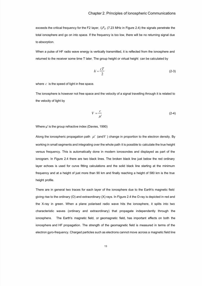
exceeds the critical frequency for the F2 layer, f o F 2 , (7.23 MHz in Figure 2.4) the signals penetrate the
total ionosphere and go on into space. If the frequency is too low, there will be no returning signal due
to absorption.
When a pulse of HF radio wave energy is vertically transmitted, it is reflected from the ionosphere and
returned to the receiver some time T later. The group height or virtual height can be calculated by
2'
cT h = (2-3)
where c is the speed of light in free space.
The ionosphere is however not free space and the velocity of a signal travelling through it is related to
the velocity of light by
'μ
cV = (2-4)
Where μ' is the group refractive index (Davies, 1990)
Along the ionospheric propagation path 'μ (andV ) change in proportion to the electron density. By
working in small segments and integrating over the whole path it is possible to calculate the true height
versus frequency. This is automatically done in modern ionosondes and displayed as part of the
ionogram. In Figure 2.4 there are two black lines. The broken black line just below the red ordinary
layer echoes is used for curve fitting calculations and the solid black line starting at the minimum
frequency and at a height of just more than 90 km and finally reaching a height of 580 km is the true
height profile.
There are in general two traces for each layer of the ionosphere due to the Earth's magnetic field
giving rise to the ordinary (O) and extraordinary (X) rays. In Figure 2.4 the O-ray is depicted in red and
the X-ray in green. When a plane polarised radio wave hits the ionosphere, it splits into two
characteristic waves (ordinary and extraordinary) that propagate independently through the
ionosphere. The Earth's magnetic field, or geomagnetic field, has important effects on both the
ionosphere and HF propagation. The strength of the geomagnetic field is measured in terms of the
electron gyro-frequency. Charged particles such as electrons cannot move across a magnetic field line

8/4/2019 Coetzee MSc Thesis
http://slidepdf.com/reader/full/coetzee-msc-thesis 25/73
Chapter 2. Principles of Ionospheric Communications
14
but are forced to spiral or rotate around them. The rate at which they rotate is called the gyro-
frequency and depends on how heavy they are, their electric charge and the strength of the magnetic
field. For electrons in the geomagnetic field, the gyro-frequency is typically less than 2 MHz and varies
with latitude and longitude over the surface of the Earth. The vertical asymptotes for f o F 2 and f x F 2 are
separated by approximately half the gyro-frequency, f b. For Grahamstown this is approximately 0.38
MHz according to Figure 2.4.
2.4 HF radio propagation
A simplified geometrical model is used to describe the aspects related to ionospheric propagation. For
illustrative purposes use is made of a flat earth and a flat ionosphere.
Figure 2.5: Simplified geometrical propagation model
In Figure 2.5 radio waves are emitted by the transmitter T at an elevation angle φ , travelling a distance
D/2 before striking the ionosphere at point P and being reflected back to Earth, arriving at the receiver
R. In reality, the ray is not reflected at P, but is continuously refracted or bent towards the ground as it
passes through the ionosphere (Devoldere, 2005). However for many practical purposes this
complexity can be ignored and it can be considered that the ray is reflected at P. The ionosphere at
Transmitter T
Reflection Point P
Earth
Receiver R
Sky Wave
GroundRange D
ReflectionHeight hElevation
Angle φ
Ionosphere
Ray Incidence Angle θ

8/4/2019 Coetzee MSc Thesis
http://slidepdf.com/reader/full/coetzee-msc-thesis 26/73
Chapter 2. Principles of Ionospheric Communications
15
the point of reflection P, is at a height h above the midpoint, M, of the circuit. The distance along the
ground between the transmitter T and the receiver, R, is called the ground range, D.
One of the most important quantities in HF communications is the maximum useable frequency or
MUF, which is the maximum frequency that will be reflected by the ionosphere for a given circuit. The
MUF is a median representation (statistical value) and not an individual value. The MUF depends on
just two things, the critical frequency, f c, of the ionosphere at the reflection point, P, and the geometry
of the circuit. The MUF is given by the formula
θ secc f MUF = (2-5)
Where θ is the ray incidence angle. Equation (2-5) is also known as the secant law (Davies, 1990).
For radio propagation purposes it is more convenient to work with the elevation angle,φ :
φ sin
c f MUF = (2-6)
Since φ sin can vary from 0 to 1, equation (2-6) indicates that the MUF is equal to the critical
frequency of the ionosphere for vertical incidence (φ = 90°, sin 90° = 1). It also indicates that the MUF
and ground range D are much higher for low elevation angles. In practice the world is round and the
curvature of the surface prevents the elevation angle from getting too close to 0°, causing the MUF
(and ground range) to reach a finite upper limit for a given ionosphere.
Equation (2-6) may be used to calculate the MUF for reflection at a given altitude in the F layer,
provided the critical frequency f c (f o F 2 ) is replaced by the plasma frequency at the reflection height,
f n (h).
)(sin
)()(
h
h f h MUF
n
φ = (2-7)
Where "h " indicates what is happening if the reflection occurs at the height h. In general, the higher the
frequency, the higher the signals must penetrate into the ionosphere to find a plasma frequency high
enough to reflect them.
8/4/2019 Coetzee MSc Thesis
http://slidepdf.com/reader/full/coetzee-msc-thesis 27/73
Chapter 2. Principles of Ionospheric Communications
16
For propagation to be possible on a given circuit, the operating frequency, f o, must be less than or
equal to the MUF for the circuit. At higher frequencies the signals would simply penetrate the
ionosphere.
It is possible to determine an Optimum Working Frequency (OWF) or Frequency Optimum de Travail
(FOT), generally referred to as the Frequency for Optimum Traffic, from the MUF. The frequency that
is equal to the lower decile value of the thirty or thirty-one individual MUFs for the month is known as
the FOT. The OWF or FOT is the internationally agreed standard for the "best" or "optimum" frequency
to use at a given hour on a given circuit. Its use will result in successful communications (at least as
far as the correct choice of frequency is concerned) on 90% or 27 days of the month (McNamara,
1991). It is possible to get an estimated value of the FOT (EFOT) by taking 85% of the basic MUF.
This is a convenient definition to calculate the FOT for a given circuit.
Under certain conditions a skip zone or dead zone may exist up to a certain distance from the
transmitter. If the operating frequency is higher than the critical frequency ( f o F 2 ), reflection will only
occur if the elevation angle is low enough to comply with Equation 2-6. It will not be possible to
communicate with stations within the skip zone unless the operating frequency is reduced to be less
than or equal to the MUF for the required distance. The skip zone for a given transmitter will depend
on the operating frequency (getting larger as the frequency increases) and the critical frequency of the
reflecting layer. The skip zone can be put to good effect if secure communications are required.
The propagation of HF signals through the ionosphere can be graphically illustrated by plotting the
ground range for all elevation angles (0 - 90°) for a specific frequency, transmitter position, time of
day, date, operating frequency and ionosphere.

8/4/2019 Coetzee MSc Thesis
http://slidepdf.com/reader/full/coetzee-msc-thesis 28/73
Chapter 2. Principles of Ionospheric Communications
17
E layer Propagation
F1 layer Propagation
F2 layer Propagation
Figure 2.6: Calculated propagation of a 5 MHz signal through the ionosphere
The IRI was used to generate the ionospheric data required to calculate the ground range for all
elevation angles as depicted in Figure 2.6. For the inputs to the IRI for the generation of Figure 2.6 the
time of the day was taken as noon UT, which is 14h00 in South Africa. The season was towards the
end of summer and the position was taken as close to Pretoria. A frequency of 5 MHz was chosen as
it was determined from practical experience that successful communications are obtained for both very
short distances (Near Vertical Incidence Signals, NVIS) and longer distances up to a few hundred
kilometres under the above described conditions. The peak layer parameters (f o E , f o F 1 and f o F 2 )
calculated by the IRI are displayed in the top, right-hand corner of Figure 2.6.
Ray-tracing techniques (McKinnell, 2002) were used to model the ray path (red graph) through the
ionosphere. The blue line is used to indicate a ground range for a specified elevation angle. Possible
propagation via two ionospheric layers can be identified: E layer propagation for elevation angles

8/4/2019 Coetzee MSc Thesis
http://slidepdf.com/reader/full/coetzee-msc-thesis 29/73
Chapter 2. Principles of Ionospheric Communications
18
between 0 and about 38° and F layer for higher elevation angles. The critical frequency of the E layer
(f o E ) is 3.21 MHz according to Figure 2.6. As the operating frequency (5 MHz) is considerably higher
than f o E , only low angle signals will be reflected by the E layer. The situation is quite different for the
F2 layer as f o F 2 is 8.69 MHz with the result that all high angle signals will be reflected back to Earth by
the F2 layer. No skip- or dead zone exists under the conditions used to generate Figure 2.6 and
ionospheric communications from very near the transmitter up to a distance of nearly 2 000 km is
possible (depending on the radiation angles of the antennas used).
E layer Propagation
F1 layer Propagation
F2 layer Propagation
Skip Zone
Figure 2.7: Calculated propagation of an 11.5 MHz signal through the ionosphere
Figure 2.7 uses the same ionospheric information, transmitter position, etc (as Figure 2.6) but now the
operating frequency is 11.5 MHz, considerably higher than the critical frequency of any of the
ionospheric layers. The E layer will support propagation for signals with elevation angles between 0
and about 13°. Above 13° the F1 and F2 layers take over up to about 48°. For elevation angles higher

8/4/2019 Coetzee MSc Thesis
http://slidepdf.com/reader/full/coetzee-msc-thesis 30/73
Chapter 2. Principles of Ionospheric Communications
19
than 48°, the 11.5 MHz signal cannot be reflected back to Earth by the ionosphere. Due to the fact that
propagation is not possible for elevation angles of higher than 48°, a skip zone of just less than 750
km exists. Communications between 0 and 750 km is thus not possible under the conditions depicted
in Figure 2.7. (Short-range ground wave propagation and line-of-sight propagation exists, but it is
beyond the scope of this study.) Also note that for distances between 1 000 and 2 000 km,
propagation via both the E and F layers are possible. If the antenna radiates most of the signal
between 0 and 30°, considerable signal fading will be experienced due to the different path lengths.
From the ray-tracing plots another propagation phenomena is also clearly illustrated: the existence of
a so-called "high-ray" or Pederson ray close to the MUF for the specific layer (Goodman, 1992).
Referring to Figure 2.7 it can be seen that for a distance of for example 1 250 km, propagation is
possible at an elevation angle of about 6°, the so-called "low E ray". But propagation over a 1 250 km
distance is also possible via the E layer at an elevation angle of about 12°, the so-called "high E ray".
A third propagation path also exists at an elevation angle of 23°, the so-called "low F ray". Once again
considerable signal fading will be experienced due to the different path lengths when the propagation
circuit is close to the MUF of one of the lower layers.
2.5 Summary
The ionosphere, especially in terms of radio propagation was discussed. The relationship between the
electron density profile and layer critical frequencies was presented. Ray tracing results for different
frequencies were presented to illustrate the most commonly used HF propagation terminology
including the MUF, FOT, skip zone, etc. In short: ionospheric propagation is not "black magic" or a
"black art" but rather a well-defined and accurate science. It would have been even more utilised and
better understood by the general public if it wasn't for the extremely dynamic nature of the ionosphere
that so often play havoc with the best frequency prediction efforts.

8/4/2019 Coetzee MSc Thesis
http://slidepdf.com/reader/full/coetzee-msc-thesis 31/73
20
Chapter 3 - Advantages of the 30 - 35 MHz Band (Compared to HF)
3.1 Introduction
The sample path for communications between South Africa (Pretoria) and Central Africa (Kisangani)
were defined in Chapter 1. The principles of the sky wave ionospheric communications that are going
to be utilised to try and fulfil the requirements of Chapter 1 were discussed in Chapter 2. The
advantages of utilising frequencies above the higher limit of the classic HF band (30 MHz) will be
investigated to determine what benefits can be expected if successful communications for the
requirements stated in Chapter 1 can be established.
3.2 Low probability of intercept
Most of the previous “traditional” users of the 30 to 35 MHz segment of the VHF band have migrated
to either the 150 to 170 MHz band or the 400 to 450 MHz UHF band. The smaller antenna sizes
associated with the higher frequencies are a big advantage to mobile users and are much preferred
over the long “whips” required for the low VHF band. At the moment the 34 MHz portion is allocated to
the remote control of model aircraft (see Appendix A for a list of frequencies) and the rest of the band
is sparsely populated. (It is a good idea to avoid operating on the model aircraft frequencies.)
Monitoring types of HF receivers as utilised by the military, intelligence, other para-statal
organisations, drug traffickers, terrorist groups, etc typically have a higher frequency limit of 30 MHz.
These receivers will thus not be able to operate on the proposed frequencies. Organisations equipped
with this type of HF receiver will thus not be able to intercept the proposed communications.
The operators of V/UHF monitoring receivers tend to listen to the higher frequencies (150 MHz or 450
MHz bands) where there is much more activity and signals of interest. The V/UHF monitoring stations
typically use vertically polarised antennas to ensure optimum reception of the mobile and other users
of the V/UHF spectrum. If the proposed communications system utilises horizontally polarised
antennas the intercepted signal strength will further be reduced by nearly 20 dB due to the polarisation
mismatch. This will further reduce the footprint of the transmitter to basically line-of-sight.

8/4/2019 Coetzee MSc Thesis
http://slidepdf.com/reader/full/coetzee-msc-thesis 32/73
Chapter 3. Advances of the 30-35 MHz Band
21
The skip or dead zone of this frequency range will extend from just beyond line-of-sight up to at least 1
500 km (as calculated in Chapter 4). This implies that it will probably not be possible to intercept the
signal via sky wave in the country that it originates from. This feature will enhance the communications
security considerably.
The proposed communications link will mostly be utilised for data communications. This will draw
much less attention than a voice link, especially if an advanced modulation scheme such as
Quadrature Amplitude Modulation (QAM) or Orthogonal Frequency Division Multiplexing (OFDM) with
online encryption is used. Casual access to the message content will then be impossible.
3.3 Low received noise
The signal-to-noise ratio of HF communications systems is limited by received (external) noise and not
by the internally generated noise of the receiver (receiver noise figure). From Figure 3.1 it can be seen
that the galactic noise at 4 MHz is nearly 40 dB above the thermal noise (noise generated by a 50 Ω
resistor at room temperature). At 30 MHz it is at least 20 dB higher than the thermal noise floor (graph
D in Figure 3.1).

8/4/2019 Coetzee MSc Thesis
http://slidepdf.com/reader/full/coetzee-msc-thesis 33/73
Chapter 3. Advances of the 30-35 MHz Band
22
0372-02
A
E
D
C
B
0
20
40
60
80
100
120
140
160
180
2 5 2 5 2 5 2 5
104
105
106
107
108
2.9 × 10¹⁰
2.9 × 10⁸
2.9 × 10²
2.9 × 10²⁰
2.9 × 10¹⁸
2.9 × 10¹⁶
2.9 × 10¹⁴
2.9 × 10¹²
2.9×
106
2.9 × 10⁴
t
( K )
a
FIGURE 2
F a versus frequency (104 to 108 Hz)
F
( d B )
a
Frequency (Hz)
ABCDE
: atmospheric noise, value exceeded 0.5% of time: atmospheric noise, value exceeded 99.5% of time: man-made noise, quiet receiving site: galactic noise: median business area man-made noise
minimum noise level expected
Figure 3.1: Received noise (from RECOMMENDATION ITU-R. pp. 372-8, Radio noise, 2003)
Receiver noise figures of less than 14 dB are very easy to achieve (and very common) at HF. These
noise figures will be more than adequate for the low VHF band as although the external noise is much
lower than at HF, it is still considerably higher than that of the receiver. A considerable increase in
received signal-to-noise ratio can be expected if the operational frequency can be increased from
typically 15 MHz to above 30 MHz (at least 10 dB according to graph D of Figure 3.1.)
3.4 Reduced interference from lightning discharges
Lightning and static discharge activity also contributes greatly to the pulse and burst type noise
interference experienced on HF. According to Figure 3.2 the equator is a region of extremely high

8/4/2019 Coetzee MSc Thesis
http://slidepdf.com/reader/full/coetzee-msc-thesis 34/73
Chapter 3. Advances of the 30-35 MHz Band
23
lightning activity, making HF communications very challenging. The energy density in the interference
generated by lightning decreases rapidly with higher frequency. The received signal-to-noise ratio will
thus increase considerably if the operating frequency can be increased as much as possible, once
again preferably beyond 30 MHz.
Figure 3.2: Worldwide lightning probability distribution (from Christian et al, 2003)
3.5 Small antennas
The wavelength of a RF signal is determined by (Braun, 1982):
F
c=λ (3-1)
Where
λ is the wavelength in metre,
c is the speed of light in metres per second
and F is the operating frequency in Hertz.

8/4/2019 Coetzee MSc Thesis
http://slidepdf.com/reader/full/coetzee-msc-thesis 35/73
Chapter 3. Advances of the 30-35 MHz Band
24
For communication purposes the following formula is normally used:
F
300=λ (3-2)
Where
λ is the wavelength in metre
and F is the operating frequency in Megahertz (MHz).
The basic antenna is the half-wave dipole. From equation (3-2) it can be calculated that the total
length of the antenna is 10 metres for an operating frequency of 15 MHz. The size of the antenna will
half (total length 5 metres) if the frequency can be increased to 30 MHz. This is a very worthwhile
improvement and makes the antenna physically much more manageable on a practical level. It is also
much easier to hide a smaller antenna from prying eyes.
3.6 High data rates
The low VHF band is traditionally a FM band. The channel spacing is typically 25 kHz and the
modulated bandwidth is limited to 15 kHz. On HF the available bandwidth of a Single Side Band (SSB)
channel is maximum 3 kHz (300 Hz – 3.3 kHz) and in many instances it is as low as 2.4 or 2.2 kHz.
Just in terms of available bandwidth it is thus possible to utilise a five times higher data rate compared
to HF. Add the lower noise floor and reduced lightning interference and the effective data throughput
will be even higher than five times when compared to a typical HF channel. In today’s age of situation
reports generated with the aid of a word processor on a computer, high data tempos are mandatory for
effective management of resources.
If advanced modulation schemes (multiple level QAM or OFDM) are implemented the data rates will
compare favourably with that offered by satellite, at a fraction of the cost. With these modulation
techniques data rates considerably higher than 1 bit per Hz is achievable.

8/4/2019 Coetzee MSc Thesis
http://slidepdf.com/reader/full/coetzee-msc-thesis 36/73
Chapter 3. Advances of the 30-35 MHz Band
25
3.6 Summary
The probability of intercept (in terms of skip zone), atmospheric noise, lightning interference, antenna
size and possible data rates for a typical VHF bandwidth was investigated. It is very clear that there
are considerable advantages compared to the classic HF band if the low VHF band can be utilised for
a communications link between Central Africa and South Africa. Advantages include higher data rates
due to the lower noise levels and wider bandwidths, less interference from lightning activity, physically
smaller antennas and higher security.

8/4/2019 Coetzee MSc Thesis
http://slidepdf.com/reader/full/coetzee-msc-thesis 37/73
26
Chapter 4 - Possible Single Hop Propagation Investigation
4.1 Introduction
The principles of ionospheric propagation as defined in Chapter 2 are now utilised to investigate the
possibility of successful communications between Pretoria (South Africa) and Kisangani (Central
Africa). Accurate ionospheric information is a pre-requisite to solve the problem as stated in Chapter 1.
There are no ionosondes available at the calculated reflection point(s). The International Reference
Ionosphere (IRI) model is thus used to generate the required ionospheric data. Firstly representative
peak layer heights, h m F 2 , are determined. With the distance for the sample communications path
known the required elevation angles can then be calculated. With the reflection heights, path distance
and elevation angles known, it is possible to calculate the required F2 layer critical frequencies (f o F
2 ).
Once the required critical frequencies are determined the IRI ionospheric model is once again utilised
to determine when (in terms of time-of-day and sunspot activity) this value is achieved (or exceeded)
at the reflection point.
4.2 F2-layer peak height (h m F 2 ) requirements
The International Reference Ionosphere 2007 (IRI) was used to determine representative peak F2
layer heights (h m F 2 ) at the reflection point between Kisangani and Pretoria namely 12.85° South and
26.61° East. The time of day was varied to investigate under what conditions ionospheric propagation
may be possible. The peak layer height is critical in determining the required elevation angle for
successful propagation. A greater height will improve the chances of success as a higher, more
practical radiation angle can then be utilised. According to the IRI recent solar cycles achieved
Smoothed Sunspot Numbers (SSN’s) of nearly 160 and minimum values of less than 5. Values of
higher than 60 are typically achieved for more than six years (> 50%) of a solar cycle.

8/4/2019 Coetzee MSc Thesis
http://slidepdf.com/reader/full/coetzee-msc-thesis 38/73

8/4/2019 Coetzee MSc Thesis
http://slidepdf.com/reader/full/coetzee-msc-thesis 39/73
Chapter 4. Possible Single Hop Propagation
28
Figure 4.2: IRI generated summer 24 hour peak layer height profile for SSN > 60 at the reflection point
(single hop scenario)
In Figure 4.2 the peak layer height was plotted over the course of a day (twenty four hours) at the
single hop reflection point between Pretoria and Kisangani. These values were determined for a
summer day at a SSN of more than 60. It can be seen that an h m F 2 value of between 350 and 360 km
is achieved during the afternoon hours.
4.3 Elevation angles for single hop propagation
With the range of h m F 2 values determined it is now possible to calculate the required elevation angles.
The ionosphere is a very dynamic medium and a large percentage of the time the operational
frequency is going to be uncomfortably close to the MUF for the sample circuit as defined in Chapter
1. It is therefore best to assume that the signal will not be reflected at a single height but rather over a
range of heights limited by the thickness of the layer. The required maximum elevation angle is
determined by the peak layer height, h m F 2 , but it can also be lower depending on the instantaneous
electron density. As the requirement is for the propagation of a relatively high frequency (>30 MHz), it

8/4/2019 Coetzee MSc Thesis
http://slidepdf.com/reader/full/coetzee-msc-thesis 40/73
Chapter 4. Possible Single Hop Propagation
29
can be assumed that when propagation is possible, reflection will most probably occur in the highest
20% of the F2 layer, in other words the densest 20% of the ionosphere.
4.4.1 Required elevation angles assuming a flat Earth
Figure 4.3: Simplified geometrical propagation model assuming a flat earth
Using the simplified propagation model depicted in Figure 4.3, the required elevation angle can be
calculated using simple geometry as:
2
tan D
h=φ (4-1)
Where φ is the required elevation angle,
h is the reflection point height (of the F2 layer)
and2
Dis half the distance between the transmitter or the receiver to the reflection point.
Using the 280 to 360 km h m F 2 values for the height as determined using the IRI and illustrated in
Figures 4.1 and 4.2. and 1 463 km for the distance to the reflection point as defined in Chapter 1, the
required elevation angles according to Equation 4-1 are between 10.8 and 13.8°.
The Earth is however not flat and for greatest accuracy use must rather be made of a curved Earth for
calculation purposes.
Transmitter T
Reflection Point P
Earth
Receiver R
Sky Wave
GroundRange D
ReflectionHeight hElevation
Angle φ
Ionosphere

8/4/2019 Coetzee MSc Thesis
http://slidepdf.com/reader/full/coetzee-msc-thesis 41/73
Chapter 4. Possible Single Hop Propagation
30
4.4.2 Required elevation angles for a curved Earth
In Appendix B a formula is derived to determine the great circle propagation distance as a function of
the reflection point height and the required elevation angle of the signal. With the required distance
and the possible reflection heights known the formula can be manipulated to determine the required
elevation angles.
The great circle propagation distance for a curved Earth can be calculated from (Elwell, 1982):
])000157.01
cos[arccos(265.222 φ
φ −
+=
ih D (4-2)
Where φ is the required elevation angle,
ih is the reflection height (of the F2 layer)
and D is the distance between the transmitter or the receiver (in km).
Once again using 280 to 360 km for ih as determined in Figures 4.1 and 4.2 and 2 927 km for the
great circle distance between the transmitter and the receiver results in required elevation angles of
between 3.6 and 6.4°.
These values differ considerably from those of the assumed flat Earth instance. For this study the
curved Earth values are considerably more appropriate and are exclusively used for all further
elevation angle calculations.
4.5 Required antenna height
Elevation angles of between 3.6 and 6.4° can be considered to be quite low. At this stage it is a good
idea to determine how realistic this requirement is. An antenna simulation program using numeric
analysis techniques called EZNEC (Lewallen, 2007) was used to determine the required height of the
antenna above ground level. The results are displayed in Figure 4.4. A simple, horizontal, half-wave
dipole antenna was modelled at 32 MHz above average ground.
The required elevation angles were achieved at a height of 23 metres above ground level and are
illustrated in Figure 4.4.

8/4/2019 Coetzee MSc Thesis
http://slidepdf.com/reader/full/coetzee-msc-thesis 42/73
Chapter 4. Possible Single Hop Propagation
31
Figure 4.4: 32 MHz horizontal dipole 23 m above ground
For permanent installations a height of 23 m can still be considered but at the other end of the link
(temporary deployment) it is going to require a dedicated mast or other very high support point. (For
the permanent side of the link use can be made of the facilities of a military base in South Africa that
already possesses a radio mast higher than 23 m.)
The possibility of double hop propagation must be investigated to determine if a higher elevation angle
and therefore more practical solution in terms of the required antenna height can be found.

8/4/2019 Coetzee MSc Thesis
http://slidepdf.com/reader/full/coetzee-msc-thesis 43/73
Chapter 4. Possible Single Hop Propagation
32
4.6 Summary
The IRI was utilised to determine the peak F2 layer height at the reflection point. The required
radiation angles for both a flat Earth and a curved Earth were calculated. There is a noticeable
difference for the instances mainly due to the curvature of the Earth and the ground distance involved.
For this study a curved Earth is exclusively used for all elevation angle calculations.
An antenna modelling program using numeric electromagnetic techniques was used to determine at
what height above the ground the required radiation angles of between 3.6 and 6.4° can be achieved.
This turned out to be at 23 m, a considerable but not insurmountable requirement for permanent
installations as many South African military bases already possess the required infrastructure. For
temporary, semi-mobile applications achieving the required height is however going to be very
challenging.
The possibility of double hop propagation must be investigated as the requirements on the elevation
angle will be considerably relaxed if double hop propagation proves to be possible.

8/4/2019 Coetzee MSc Thesis
http://slidepdf.com/reader/full/coetzee-msc-thesis 44/73
33
Chapter 5 - Possible Double Hop Propagation Investigation
5.1 Introduction
In Chapter 4 it was determined that single hop; low VHF propagation may be possible between
Pretoria and Kisangani but that an elevation angle of between 3.6 and 6.4 ° will be required. These low
elevation angles necessitate the antennas to be at a height of 23 m, a considerable practical challenge
for semi-mobile, rapid deployment types of operation. In this chapter the possibility of double hop
propagation for the sample path is going to be investigated. Double hop propagation will require higher
elevation angles, easing the requirements on antenna heights and making the communications link
more suitable for semi-mobile and rapid deployment operations.
If one end of the link is located at Kisangani (0.25° North, 25.12° East) and the other at Pretoria
(25.45° South, 28.10° East), the signal will be reflected at 6.18° South, 25.87° East and at 19.03°
South, 27.36° East for double hop communications. The great circle distance from the
transmitter/receiver to the ionospheric reflection points is thus 732 km. This simplified double hop
scenario is depicted in Figure 5.1. For illustrative purposes use is made of a flat earth and a flat
ionosphere.
Figure 5.1: Simplified double hop scenario
Kisangani
(0.25° N,
25.12° E)
Ionosphere
Earth
Pretoria
(25.45° S,
28.10° E)
Signal Path
ReflectionPoint 1
(6.18° S,
25.87° E)
ReflectionPoint 2
(19.03° S,
27.36° E)
1 464 km

8/4/2019 Coetzee MSc Thesis
http://slidepdf.com/reader/full/coetzee-msc-thesis 45/73
Chapter 5. Possible Double Hop Propagation
34
Once again the IRI was used to determine the peak layer heights at the reflection points.
5.2 Most Northerly reflection point
In Figure 5.2 the peak layer height was plotted over the course of a day (twenty four hours) at the most
Northerly reflection point between Pretoria and Kisangani. These values were calculated for a winter
day at a SSN of more than 60. It can be seen that h m F 2 values of between 290 and nearly 325 km are
achieved during the afternoon hours.
Figure 5.2: IRI generated winter 24 hour peak layer height profile for SSN > 60 at the most northerly
reflection point (double hop scenario)
In Figure 5.3 the peak layer height was plotted over the course of a day (twenty four hours) at the most
Northerly reflection point between Pretoria and Kisangani. These values were calculated for a summer
day at a SSN of more than 60. It can be seen that h m F 2 values of between 380 and 390 km are
achieved during the afternoon hours.

8/4/2019 Coetzee MSc Thesis
http://slidepdf.com/reader/full/coetzee-msc-thesis 46/73
Chapter 5. Possible Double Hop Propagation
35
Figure 5.3: IRI generated summer 24 hour peak layer height profile for SSN > 60 at the most northerly
reflection point (double hop scenario)
5.3 Most Southerly reflection point
In Figure 5.4 the peak layer height was plotted over the course of a day (twenty four hours) at the most
Southerly reflection point between Pretoria and Kisangani. These values were calculated for a winter
day at a SSN of more than 60. It can be seen that h m F 2 values of between 260 and 275 km are
achieved during the afternoon hours.

8/4/2019 Coetzee MSc Thesis
http://slidepdf.com/reader/full/coetzee-msc-thesis 47/73
Chapter 5. Possible Double Hop Propagation
36
Figure 5.4: IRI generated winter 24 hour peak layer height profile for SSN > 60 at the most southerly
reflection point (double hop scenario)
In Figure 5.5 the peak layer height was plotted over the course of a day (twenty four hours) at the most
Southerly reflection point between Pretoria and Kisangani. These values were calculated for a summer
day at a SSN of more than 60. It can be seen that h m F 2 values of between 325 and 345 km are
achieved during the afternoon hours.

8/4/2019 Coetzee MSc Thesis
http://slidepdf.com/reader/full/coetzee-msc-thesis 48/73
Chapter 5. Possible Double Hop Propagation
37
Figure 5.5: IRI generated summer 24 hour peak layer height profile for SSN > 60 at the most Southerly
reflection point (double hop scenario)
The lowest required elevation angle for double hop propagation will be determined by the lowest peak
layer height. From Figure 5.4 it was determined to be at the most Southerly reflection point during the
winter.
5.4 Required elevation angles assuming a curved Earth
From Appendix B the distance formula for a curved Earth is (Elwell, 1982):
])000157.01
cos[arccos(265.222 φ
φ −
+=
ih D (5-1)
Using the most Southerly reflection points’ h m F 2 values of 260 to 345 km (as determined in Figures 5.4
and 5.5) and 1 464 km for the great circle distance between the transmitter and the reflection point on
the Earth results in required elevation angles of between 15.9 and 21.3°.
8/4/2019 Coetzee MSc Thesis
http://slidepdf.com/reader/full/coetzee-msc-thesis 49/73
Chapter 5. Possible Double Hop Propagation
38
These elevation angle values are considerably more achievable with modest antenna heights than
those required by the single hop instance.
5.5 Required critical frequency (f o F 2 ) for double hop propagation
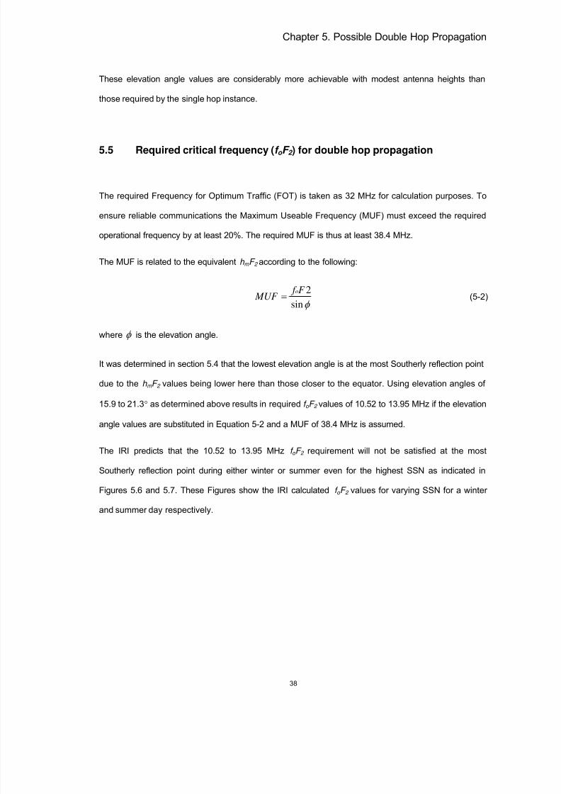
The required Frequency for Optimum Traffic (FOT) is taken as 32 MHz for calculation purposes. To
ensure reliable communications the Maximum Useable Frequency (MUF) must exceed the required
operational frequency by at least 20%. The required MUF is thus at least 38.4 MHz.
The MUF is related to the equivalent h m F 2 according to the following:
φ sin
2F f MUF
o= (5-2)
where φ is the elevation angle.
It was determined in section 5.4 that the lowest elevation angle is at the most Southerly reflection point
due to the h m F 2 values being lower here than those closer to the equator. Using elevation angles of
15.9 to 21.3° as determined above results in required f o F 2 values of 10.52 to 13.95 MHz if the elevation
angle values are substituted in Equation 5-2 and a MUF of 38.4 MHz is assumed.
The IRI predicts that the 10.52 to 13.95 MHz f o F 2 requirement will not be satisfied at the most
Southerly reflection point during either winter or summer even for the highest SSN as indicated in
Figures 5.6 and 5.7. These Figures show the IRI calculated f o F 2 values for varying SSN for a winter
and summer day respectively.

8/4/2019 Coetzee MSc Thesis
http://slidepdf.com/reader/full/coetzee-msc-thesis 50/73
Chapter 5. Possible Double Hop Propagation
39
Figure 5.6: IRI generated winter f o F 2 for all SSN at the most Southerly reflection point (double hop
scenario)

8/4/2019 Coetzee MSc Thesis
http://slidepdf.com/reader/full/coetzee-msc-thesis 51/73
Chapter 5. Possible Double Hop Propagation
40
Figure 5.7: IRI generated summer f o F 2 for all SSN at the most Southerly reflection point (double hop
scenario)
Communication via double hop propagation is thus not a viable option for the path required.
5.6 Summary
The possibility of double hop propagation between Pretoria and Kisangani was investigated. The IRI
was utilised to determine the peak F2 layer heights at both the reflection points. The required radiation
angles for a curved Earth were calculated and found to be at a very achievable 15.9 to 21.3 °. When
the required MUF’s were calculated for the double hop propagation distances and heights as defined
in Figure 5.1, it was found that the corresponding f o F 2 requirements are not met at the most Southerly
reflection point. Double hop propagation is thus (unfortunately) not possible and the most probable
solution is thus the single hop propagation scenario investigated in Chapter 4.

8/4/2019 Coetzee MSc Thesis
http://slidepdf.com/reader/full/coetzee-msc-thesis 52/73
41
Chapter 6 - Sample Communication Solution
6.1 Introduction
Antenna height can still be controlled but the f o F 2 value is a natural occurrence totally beyond man’s
control. The only possible solution is therefore single hop propagation using antenna heights of ≥ 23 m
at both ends of the link as determined in Chapters 4 and 5. The other applicable parameters (f o F 2 , skip
zone, transmitter power requirements, path loss, etc) must be calculated to determine if the
requirements for the sample path of Chapter 1 can be met with single hop propagation.
6.2 Required critical frequency (f o F 2 ) for single hop communications
The required Frequency for Optimum Traffic (FOT) is taken as 32 MHz. To ensure reliable
communications the Maximum Useable Frequency (MUF) must exceed the required operational
frequency by at least 20%. The required MUF is thus at least 38.4 MHz.
The MUF is related to the equivalent f o F 2 according to the following:
φ sin
2F f MUF
o= (6-1)
where φ is the elevation angle.
Using elevation angles of 3.6 to 6.4° as determined in Chapter 4 results in required f o F 2 values of 2.4
and 4.28 MHz. These values are exceeded on a daily basis during the daytime at the single hop
reflection point whenever the SSN exceeds 15 as indicated in Figure 6.1.

8/4/2019 Coetzee MSc Thesis
http://slidepdf.com/reader/full/coetzee-msc-thesis 53/73
Chapter 6. Sample Communication Solution
42
Figure 6.1: IRI generated winter f o F 2 for all SSN at the reflection point (single hop scenario)
The IRI was once again utilised to determine the times of the day that the required f o F 2 value of 4.28
MHz are exceeded (for the single hop scenario) with a SSN of 15. The results are displayed in Figure
6.2.

8/4/2019 Coetzee MSc Thesis
http://slidepdf.com/reader/full/coetzee-msc-thesis 54/73
Chapter 6. Sample Communication Solution
43
Figure 6.2: IRI generated winter f o F 2 for an SSN > 15 at the reflection point (single hop scenario)
The single hop propagation requirement of a f o F 2 > 4.28 MHz with a SSN > 15 is basically met during
all daylight hours during the winter according to Figure 6.2.
6.3 Skip or dead zone
From equation (6-1) it is also possible to determine the highest elevation angle that will be reflected by
the F2 layer of the ionosphere for the operating frequency (32 MHz). For a f o F 2 of 2.4 MHz the highest
elevation angle is 4.3° and for 4.28 MHz it is 7.7°. These angles translate to skip distances of between
2 992 km and 2 476 km for an ionospheric height of 300 km.
These distances ensure that it is not possible to receive the signal in the country of origin (except for
short distance, line-of-sight or ground wave propagation). It only becomes possible to receive the
signal close to its intended reception area.

8/4/2019 Coetzee MSc Thesis
http://slidepdf.com/reader/full/coetzee-msc-thesis 55/73
Chapter 6. Sample Communication Solution
44
6.4 Propagation via the E layer
According to the IRI the critical frequency of the E layer exceeds 2.4 MHz regularly during high solar
activity as indicated in Figure 6.3.
Figure 6.3: IRI generated winter f o E for an SSN > 100 at the reflection point (single hop scenario)
If the height of the E layer is taken as 110 km and using an elevation angle of 3.6°, a skip distance of 1
680 km results. For an elevation angle of 6.4° the skip distance is 1 320 km. Multi-hop, E-layer
propagation will therefore occur on a regular basis during high solar activity, resulting in fading of the
received signal. This is due to the different path lengths between the single hop F2 layer and the multi-
hop, E-layer propagation modes.

8/4/2019 Coetzee MSc Thesis
http://slidepdf.com/reader/full/coetzee-msc-thesis 56/73
Chapter 6. Sample Communication Solution
45
6.5 Antenna and transmitter power requirements
A simple, low cost antenna solution will go a long way to help the operator that must deploy under
non-ideal conditions. The basic half wave dipole is mechanically very simple and also a very efficient
radiator. A dipole antenna is designed using the following equations:
Firstly determine the free space wavelength for the operating frequency:
F
300=λ (6-2)
Where
λ is the wavelength in metre
and F is the operating frequency in Megahertz (MHz).
For an operating frequency of 32 MHz the free space wavelength is 9.38 metre. The total length of the
dipole antenna, l in Figure 6.4, is half of this, or 4.69 metre. Each leg of the dipole is half of this, or
2.35 meter. The legs of a physical dipole are typically shorter than this due to the capacitive effects of
the Earth. For practical applications a length of 90% of the calculated values produces good results.
Figure 6.4: Basic half-wave dipole antenna
Feed Point(Coaxial
Cable
Length l
(λ/2)

8/4/2019 Coetzee MSc Thesis
http://slidepdf.com/reader/full/coetzee-msc-thesis 57/73
Chapter 6. Sample Communication Solution
46
6.5.1 Undesired high angle radiation
From the antenna simulation results (as shown in Figure 6.5) it is clear that there are multiple,
unwanted high angle lobes. The high angle lobes are due to ground reflections. These lobes
contribute nothing to the wanted signal and only add atmospheric noise to the received signal.
Figure 6.5: Unwanted, high angle radiation of a single dipole 23 m above ground level
The received Signal-to-Noise Ratio (SNR) can be improved if the magnitude of these high angle
responses can be reduced. The easiest way to accomplish this is to add the signal of another identical
antenna in phase to that of the existing antenna.

8/4/2019 Coetzee MSc Thesis
http://slidepdf.com/reader/full/coetzee-msc-thesis 58/73
Chapter 6. Sample Communication Solution
47
Figure 6.6: Radiation pattern of two horizontal dipoles at 18 and 23 m fed in phase
Figure 6.6 indicates that stacking two dipoles vertically (and feeding them in phase) reduces the
unwanted high angle radiation considerably. The gain has also increased from 8 to nearly 11.8 dBi
(ground reflections included), a very worthwhile improvement indeed. (The gain is referenced to that of
an isotropic antenna). The second dipole was added below the first one thus not requiring extending
the mast height.
6.5.2 Antenna polarisation
The option of using a simple, elevated, quarter-wave vertical antenna with an elevated ground plane
was also investigated and the result is displayed in Figure 6.7.

8/4/2019 Coetzee MSc Thesis
http://slidepdf.com/reader/full/coetzee-msc-thesis 59/73
Chapter 6. Sample Communication Solution
48
Figure 6.7: Radiation pattern of a quarter-wave vertical antenna 5 m above ground level
From Figure 6.7 it is clear that the (stacked) dipole antenna is far superior to a quarter-wave vertical
for this application. The gain of the vertical antenna is more than 8 dB down compared to the dipole
and there is also considerable, undesirable high angle radiation.
6.5.3 Path loss
To be able to determine the received signal power it is necessary to calculate the total path loss. The
path loss is determined by the free space losses as well as the reflection losses.
The free space path loss can be calculated from (Braun, 1982):
Ploss = 32.5 + 20 Log F + 20 Log D (6-3)
Where

8/4/2019 Coetzee MSc Thesis
http://slidepdf.com/reader/full/coetzee-msc-thesis 60/73
Chapter 6. Sample Communication Solution
49
Ploss is the free pace path loss in dB,
F is the frequency in Megahertz. In this case 32 MHz and
D is the distance in kilometres.
If the height of the reflection point is taken as 350 km and the distance to the reflection point as 1 464
km, the distance travelled by the signal to the reflection point can be calculated using Pythagoras’
equation. In this case it works out at twice 1 505 km; in total 3 010 km.
Substituting the values in Equation 6-3 results in a free space path loss of 132.2 dB.
The reflection loss between the two positions is between 3 and 6 dB (if there is propagation)
(Goodman, 1992).
In the worst case the total path loss is 138.2 dB. Path loss is a natural occurrence and it is not possible
for man to change it. The design of the other components of the communications system (e.g. antenna
gain, transmitter power, bandwidth, etc) will have to overcome this loss.
6.5.4 Expected Received Power Level
The received power can be calculated from (Goodman, 1992):
PRX = PTX + GTX ANT + GRX ANT – Ploss (6-4)
Where
PRX is the received power in Decibel referenced to one milliWatt (dBm),
PTX is the transmitter power in dBm,
GTX ANT is the transmitter antenna gain. If a dipole at a height of 23 m is used this value is 7.77 dBi as
calculated in Figure 6.5,
GRX ANT is the receiver antenna gain. If a dipole at a height of 23 m is used this value is once again 8
dBi as calculated in Figure 6.5.
Ploss is the total path loss as calculated with the aid of Equation 6.3 (138.2 dB).

8/4/2019 Coetzee MSc Thesis
http://slidepdf.com/reader/full/coetzee-msc-thesis 61/73
Chapter 6. Sample Communication Solution
50
A transmitter power level of 10 Watt is assumed as this is a common value for easily available
commercial equipment. This translates to + 40 dBm.
Substituting the above values in Equation 6-4 results in a received power level of – 82.2 dBm.
Additional system losses e.g. that of the coaxial feed lines are ignored.
6.5.5 Expected Received Signal-to-Noise Ratio
The receiver noise floor can be calculated by (Goodman, 1992):
RXNF = -174 + 10 Log BW + RXNoise Figure (6-5)
Where
-174 dBm is the thermal noise power in a 1 Hz bandwidth at 25°C,
BW is the receiver bandwidth in Hz and
RXNoise Figure is the receiver noise figure in dB.
The receiver bandwidth can be taken as 15 kHz and the noise figure as 12 dB. Substituting these
values in Equation 6-5 yields a receiver noise floor of -120 dBm. According to Figure 3.1 the expected
noise floor is -110 dBm due to the atmospheric noise. The sensitivity of the system is thus externally
limited and not by the receiver’s noise figure (internally generated noise).
With a received power level of – 82.2 dBm the expected SNR is 27.8 dB. This is a very useable value
and will ensure high data rates.
It is possible to increase the SNR by either using higher transmitter power or using higher gain (more
complex) antennas at one end of the sample propagation path. At many of the South African military
bases there are already existing high gain directional antennas (Log-Periodic dipoles), mounted on
suitably high masts. If one of these is utilised it will be very beneficial and will increase the reliability of
the communications link.

8/4/2019 Coetzee MSc Thesis
http://slidepdf.com/reader/full/coetzee-msc-thesis 62/73
Chapter 6. Sample Communication Solution
51
6.6 Validation of results
In order to validate this study, ray tracing through the ionosphere over the path considered in the study
was carried out using an analytic, path segmented, quasi parabolic ray tracing approach (Norman and
Cannon, 1997, 1999). This ray tracing approach uses the Parameterised Ionospheric Model (PIM) as
a source of ionospheric data (electron density profile) for its advanced ray-tracing algorithm. Although
most ray tracing algorithms cannot calculate path loss or expected received SNR’s, they provide an
ideal tool to independently verify the propagation results obtained from first principles in the preceding
chapters that used the IRI as a source of ionospheric data. Using this ray tracing approach the
summer scenario for medium (SSN = 15) and high (SSN = 100) solar activity was evaluated.
Figure 6.8: Ray tracing results between Pretoria and Kisangani for a SSN of 15 at 12h00 UT

8/4/2019 Coetzee MSc Thesis
http://slidepdf.com/reader/full/coetzee-msc-thesis 63/73
Chapter 6. Sample Communication Solution
52
According to the ray tracing results single hop communications between Pretoria and Kisangani is
possible from about 07h00 till 13h00 UT when the SSN is fifteen as indicated in Figure 6.8. Colours
are used to indicate the electron density for the path between Pretoria and Kisangani. The “cooler”
colours (shades of blue) indicate the least amount of free electrons while the “hot” colours (shades of
red) indicate the highest electron density. The vertical scale of Figure 6.8 is the height of the
ionosphere in kilometres. The E layer starts at a height of approximately 100 km and the peak of the F
layer is at approximately 300 kilometres. Pretoria is taken as the transmitting station and is at the
origin of the graph (on the left). The higher electron density closer to the equator as compared to that
over Southern Africa is clearly illustrated by the colour scheme. Ray paths for elevation angles of
between 1 and 15° are indicated by the black lines. The target (Kisangani) at a range of just more than
three thousand kilometres is indicated by an asterisk (*).
It was found that propagation at 32 MHz is possible for SSN’s as low as fifteen, but only for a short
period of time at around 09h00. Under no circumstances is double hop propagation possible over the
three thousand kilometre path. A skip zone of more than 2 500 km also exists during times that
propagation is possible.

8/4/2019 Coetzee MSc Thesis
http://slidepdf.com/reader/full/coetzee-msc-thesis 64/73
Chapter 6. Sample Communication Solution
53
Figure 6.9: Ray tracing results between Pretoria and Kisangani for a SSN of 100 at 08h00 UT
During high solar activity (SSN = 100) propagation is possible from 07h00 till 10h00 UT as illustrated
in Figure 6.9. After 10:00 the f o E rises to values that reflect the very low elevation angle 32 MHz signal
back into space. The E layer thus prevents the signal from reaching the target area. This effect was
not anticipated.
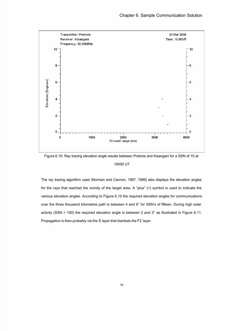
8/4/2019 Coetzee MSc Thesis
http://slidepdf.com/reader/full/coetzee-msc-thesis 65/73
Chapter 6. Sample Communication Solution
54
Figure 6.10: Ray tracing elevation angle results between Pretoria and Kisangani for a SSN of 15 at
10h00 UT
The ray tracing algorithm used (Norman and Cannon, 1997, 1999) also displays the elevation angles
for the rays that reached the vicinity of the target area. A “plus” (+) symbol is used to indicate the
various elevation angles. According to Figure 6.10 the required elevation angles for communications
over the three thousand kilometres path is between 4 and 6° for SSN’s of fifteen. During high solar
activity (SSN = 100) the required elevation angle is between 2 and 3° as illustrated in Figure 6.11.
Propagation is then probably via the E layer that blankets the F2 layer.
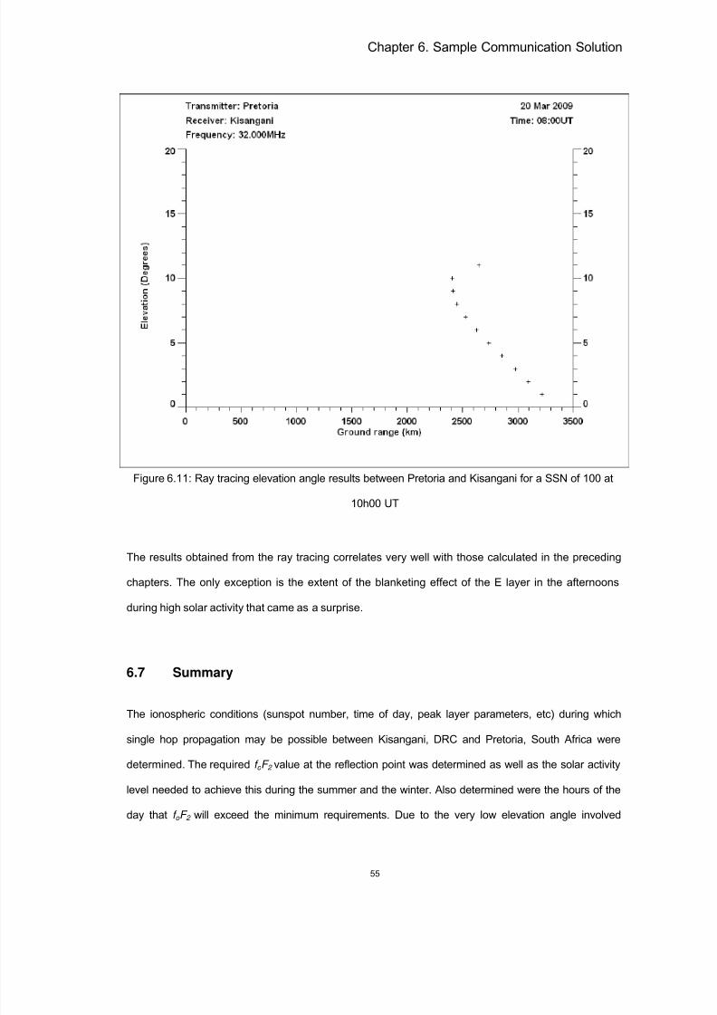
8/4/2019 Coetzee MSc Thesis
http://slidepdf.com/reader/full/coetzee-msc-thesis 66/73
Chapter 6. Sample Communication Solution
55
Figure 6.11: Ray tracing elevation angle results between Pretoria and Kisangani for a SSN of 100 at
10h00 UT
The results obtained from the ray tracing correlates very well with those calculated in the preceding
chapters. The only exception is the extent of the blanketing effect of the E layer in the afternoons
during high solar activity that came as a surprise.
6.7 Summary
The ionospheric conditions (sunspot number, time of day, peak layer parameters, etc) during which
single hop propagation may be possible between Kisangani, DRC and Pretoria, South Africa were
determined. The required f o F 2 value at the reflection point was determined as well as the solar activity
level needed to achieve this during the summer and the winter. Also determined were the hours of the
day that f o F 2 will exceed the minimum requirements. Due to the very low elevation angle involved

8/4/2019 Coetzee MSc Thesis
http://slidepdf.com/reader/full/coetzee-msc-thesis 67/73
Chapter 6. Sample Communication Solution
56
single hop propagation is possible under moderate solar activity (SSN > 15) during the daylight hours
around 10h00 UT. The skip zone and possible E layer propagation, expected path losses, receiver
noise floor and received SNR were calculated for a transmitter power of 10 Watts and dipole antennas
at a height of 23 m at both sides of the sample path. A very useful SNR of 27.8 dB can be expected
when propagation is possible.
The results were verified with the aid of a ray tracing implementation using the Parameterized
Ionospheric Model and the results agreed very well with those obtained from first principles and using
the IRI as a source of ionospheric data.
8/4/2019 Coetzee MSc Thesis
http://slidepdf.com/reader/full/coetzee-msc-thesis 68/73
57
Chapter 7 – Conclusion and Discussion
According to the above study reliable, single hop propagation of signals between 30 and 35 MHz is
possible between South Africa and Central Africa under moderate to high solar activity (Smoothed sun
spot numbers higher than 15). This opens exciting research and implementation opportunities.
7.1 Conclusion
Double hop propagation requires unrealistically high f o F 2 values for a reflection point so far south. For
all practical purposes this type of propagation can be discarded as a viable solution to the
requirement.
The probability of reliable propagation is better at the lower end (close to 30 MHz) of the VHF
frequency range. Frequencies just above 30 MHz are therefore preferable to increase the probability
of successful communications while at the same time reaping all the benefits of operating in the low
VHF frequency range (as discussed in Chapter 3).
The study determined that single hop propagation on 32 MHz is possible during daytime if the SSN is
greater than 15. This is a very modest requirement and is attainable for more than 75% of a typical
solar cycle. The very low required elevation angles (3.6 to 6.4°) are critical to the possible success of
the sample propagation path.
A horizontal dipole antenna needs to be 23 m above ground level to radiate most of the energy at
these required elevation angles. It is also a simple matter to vertically stack two dipoles spaced 5 m
apart (and feed them in phase). The bottom dipole will thus be at 18 m and the top dipole at 23 m
above ground level. The stacking reduces the undesirable high angle radiation, increases the gain,
reduces the noise temperature of the antenna and also increases the received SNR.
With a transmitter output power of 10 Watt and dipole antennas at both ends a SNR of 27.8 dB can be
expected. This is quite adequate for serious data tempos (in HF terms) in the assumed 15 kHz
bandwidth.

8/4/2019 Coetzee MSc Thesis
http://slidepdf.com/reader/full/coetzee-msc-thesis 69/73
Chapter 7. Conclusion and Discussion
58
Multi-hop, E layer propagation will occur during high solar activity (SSN > 100) and will result in fading
of the received signal due to the different path lengths.
If the proposed data link is utilised and with proper scheduling and planning it can lead to substantial
cost savings compared to satellite communications. It can also function as a predictable and reliable
back-up communications link. From the above study it is clearly a worthwhile option.
7.2 Future work
Future work may include the installation of a 32 MHz beacon transmitter (and antenna at a height of
23 m) at Kisangani (or another suitable Central Africa location) and a suitable receiver (and antenna
setup) in South Africa. The received signal strengths, smoothed sunspot numbers and other applicable
parameters (geomagnetic indices, season, etc) can be logged at regular intervals to determine how
well the predicted results of this study agree with measured values.
Recently the frequency range of 40.675 to 40.685 MHz was made available by the Independent
Communications Authority of South Africa (ICASA) for propagation research by radio amateurs. This
opens the door for South African radio amateurs and physicists to participate in low VHF propagation
research in conjunction with radio amateurs and physicists in other parts of the world. The collected
data may prove very valuable for the verification of future computer programs and ionospheric models.
The work of this study can also be incorporated in a computer program to determine the possibilities of
other low VHF ionospheric propagation paths not currently supported in freely available frequency
prediction programs. A graphical indication of the skip or dead zone and expected received SNR’s will
enhance the usefulness of such a program to military and other users not possessing a suitable
physics background.

8/4/2019 Coetzee MSc Thesis
http://slidepdf.com/reader/full/coetzee-msc-thesis 70/73
59
Appendixes
Appendix A: South African Aircraft Modelling Association’s (SAAMA)frequencies
35,000 MHz35,010 MHz
35,020 MHz35,030 MHz35,040 MHz35,050 MHz 35,060 MHz35,070 MHz35,080 MHz35,090 MHz35,100 MHz35,110 MHz35,120 MHz35,130 MHz35,140 MHz35,150 MHz
35,160 MHz35,170 MHz35,180 MHz35,190 MHz35,200 MHz35,210 MHz35,220 MHz35,230 MHz35,240 MHz35,250 MHz35,260 MHz35,270 MHz35,280 MHz35,290 MHz35,300 MHz35,310 MHz35,320 MHz35,330 MHz35,340 MHz35,350 MHz35,360 MHz35,370 MHz35,380 MHz35,390 MHz35,400 MHz35,410 MHz35,420 MHz35,430 MHz35,440 MHz35,450 MHz35,470 MHz35,480 MHz35,490 MHz35,500 MHz

8/4/2019 Coetzee MSc Thesis
http://slidepdf.com/reader/full/coetzee-msc-thesis 71/73
Appendixes
60
Appendix B: Derivation of propagation-distance formula [Elwell, 1982]
(Elwell, 1982)
Transmitter A
Ionosphere
Earth's Surface
Receiver
D
B
Center of the Earth
C
φ
hi
Re
θ/2
Figure B.1: Geometry for derivation of propagation-distance formula for a curved Earth
Figure B.1 shows the transmitting point at A, a reflection from the ionosphere at point B and a one-hop
return to Earth at point D. The virtual height of the ionosphere is h i and the average radius of the
Earth, Re, is a constant of 6 367.45 km. The intersection of the radius line from the centre of the Earth
to its surface forms a right angle at point A. The vertical angle of radiation, φ , is an angle that is added
to 90° when determining angle CAB. The distance, AD, along any great circle on the surface of the
Earth is given by:
θ eR= D (B-1)
When θ is expressed in radian, or:
θ )296.57
R(
e= D (B-2)
When θ is expressed in degrees.

8/4/2019 Coetzee MSc Thesis
http://slidepdf.com/reader/full/coetzee-msc-thesis 72/73
Appendixes
61
The problem is to find a relationship of θ with respect to φ and hi and involves the triangle CABC.
Two sides of that triangle are known: BC = Re + hi ; CA = Re.
Angle CAB is known: Angle CAB = 90° + φ = angle A.
Knowing two sides and one angle, the other side and angles may be determined from the law of sines.
Solution of problem by the law of sines.
The law of sines says, given A, φ and b (see Figure B.1):
Angle C = 180° - Angle A - Angle B (B-3)
= Angle BCA
=
2
θ
Also, = B
b
sin
A
a
sin, thus )
sinarcsin(
φ
Ab B =
And )90(180 φ +°−°=C - )sin
arcsin(φ
Ab
Replacing the above with the symbols from Figure B.1:
]Re
)90sin(Rarcsin[)90(180
2
e
ih+
+°−+°−°=
φ φ
θ
φ φ θ −+
+°−°= ]R
)90sin(Rarcsin[902 e
e
ih
But φ φ cos)90sin( =+°
And ]R
)90sin(Rarccos[]
R
)90sin(Rarcsin[90
e
e
e
e
ii hh +
+°=
+
+°−°
φ φ
Therefore φ φ
θ −+
= ]R
cosRarccos[2
e
e
ih
Knowing θ , D can now be solved and cleaning up the cos-1
term results in:
])
R1
cos[arccos(296.57R2
e
eφ φ −
+
=ih
D
But Re = 6 367.45 km.
Therefore:
])000157.01
cos[arccos(265.222 φ
φ −
+=
ih D km. (B-4)

8/4/2019 Coetzee MSc Thesis
http://slidepdf.com/reader/full/coetzee-msc-thesis 73/73
References
Bilitza, D., International Reference Ionosphere 2000, Radio Science, 36, #2, pp. 261 - 275, 2001.
Braun, G., Planning and Engineering of Shortwave Links , Siemens Aktiengesellschaft, Heyden & Son
Ltd., London, 1982.
Coetzee, P. J., Applications of the IRI (International Reference Ionosphere) in Southern Africa,
Advances in Space Research, 34 (4). pp. 2075-2079, 2004.
Christian, H. J., Blakeslee, R. J., Boccippio, D. J., Boeck, W. L., Buechler, D. E., Driscoll, K. T.,
Goodman, S. J., Hall, J. M., Koshak, W. J., Mach, D. M. and Stewart, M. F., Global distribution and
frequency of lightning as observed from space by the Optical Transient Detector , Journal of
Geophysical Research , 108, No. D1, pp. 4005, doi:10.1029/2002JD002347, 2003.
DARC Verlag, Rothammels Antennen Buch, Hessedruck, Baunatal, 2002.
Davies, K,, Ionospheric Radio, Peter Peregrinus Ltd., London, United Kingdom, 1990.
Devoldere, J., ON4UN's Low-Band Dxing, The ARRL, Inc., USA, 2005.
Elwell, H. G., Antenna geometry for optimum performance, Ham Radio Magazine , pp. 60 – 67, May
1982.
Goodman, J. M., HF Communications Science and Technology , Van Nostrand Reinhold, New York,
1992.
Lewallen, R. W., EZNEC v.4.0.39. www.eznec.com. 2007.
McKinnell, L. A., A Neural Network based Ionospheric model for the bottomside electron density profile
over Grahamstown South Africa, PhD thesis of Rhodes University, Grahamstown, 2002.
McNamara, L. F., The Ionosphere: Communications, Surveillance, and Direction Finding, Krieger
Publishing Company, Malabar, Florida, 1991.
Related Documents