Climate simulations for 1880��2003 with GISS modelE

� of 37

Climate simulations for 1880-2003 with GISS modelEJ. Hansen�,2, M. Sato2, R. Ruedy3, P. Kharecha2, A. Lacis�,4, R. Miller�,5, L. Nazarenko2, K. Lo3,G.A. Schmidt�,4, G. Russell�, I. Aleinov2, S. Bauer2, E. Baum6, B. Cairns5, V. Canuto�,M. Chandler2, Y. Cheng3, A. Cohen6, A. Del Genio�,4, G. Faluvegi2, E. Fleming7, A. Friend8,T. Hall�,5, C. Jackman7, J. Jonas2, M. Kelley8, N.Y. Kiang�, D. Koch2,9, G. Labow7, J. Lerner2,S. Menon�0, T. Novakov�0, V. Oinas3, Ja. Perlwitz5, Ju. Perlwitz2, D. Rind�,4, A. Romanou�,4,R. Schmunk3, D. Shindell�,4, P. Stone��, S. Sun�,��, D. Streets�2, N. Tausnev3, D. Thresher4,N. Unger2, M. Yao3, S. Zhang2

�NASA Goddard Institute for Space Studies, 2880 Broadway, New York, New York, USA.2Columbia University Earth Institute, New York, New York, USA.3Sigma Space Partners LLC, New York, New York, USA.4Department of Earth and Environmental Sciences, Columbia University, New York, New York, USA.5Department of Applied Physics and Applied Mathematics, Columbia University, New York, New York, USA.6Clean Air Task Force, Boston, Massachusetts, USA.7NASA Goddard Space Flight Center, Greenbelt, Maryland, USA.8Laboratoire des Sciences du Climat et de l’Environnement, Orme des Merisiers, Gif-sur-Yvette Cedex, France.9Department of Geology, Yale University, New Haven, Connecticut, USA.�0Lawrence Berkeley National Laboratory, Berkeley, California, USA.��Massachusetts Institute of Technology, Cambridge, Massachusetts, USA.�2Argonne National Laboratory, Argonne, Illinois, USA.

Corresponding author: James Hansen, [email protected], �-2�2-678-5500.

Submitted to Climate Dynamics.

Revised draft of � February 2007.

2 of 37

HANSEN ET AL.: CLIMATE SIMULATIONS FOR 1880-2003 WITH GISS MODEL E

2006) in an analysis of potential “dangerous anthropogenic in-terference” with climate. Detailed diagnostics for several of these simulations are available from the repository for IPCC runs (www-pcmdi.llnl.gov/ipcc/about_ipcc.php). Diagnostics for all of these runs, in-cluding convenient graphics, are available at data.giss.nasa.gov/modelE/transient. Sect.2defines theclimatemodelandsummarizesprinci-palknowndeficiencies.Sect.3definestime-dependentclimateforcings and discusses uncertainties. Sect. 4 considers alterna-tive ways of sampling the model’s simulated temperature change for comparison with imperfect observations. Sect. 5 compares simulated and observed climate change for �880-2003, focus-ing on temperature change but including other climate variables. Sect. 6 summarizes the capabilities and limitations of the cur-rent simulations and suggests efforts that are needed to improve future capabilities.2. Climate Model

2.1. Atmospheric Model The atmospheric model employed here is the 20-layer ver-sion of GISS modelE (2006) with 4°×5° horizontal resolution. This resolution is coarse, but use of second-order moments for numerical differencing improves the effective resolution for the transport of tracers. The model top is at 0.� hPa. Minimal drag is applied in the stratosphere, as needed for numerical stability, without gravity wave modeling. Stratospheric zonal winds and temperature are generally realistic (Fig. �7 in Efficacy 2005), but the polar lower stratosphere is as much as 5-�0°C too cold in the winter and the model produces sudden stratospheric warm-ings at only a quarter of the observed frequency. Model capabili-ties and limitations are described in Efficacy (2005) and modelE (2006).Deficienciesaresummarizedbelow(Sect.2.4).2.2. Ocean Representations We find it instructive to attach the identical atmosphericmodel to alternative ocean representations. We make calcula-tions with time-dependent �880-2003 climate forcings with the atmosphere attached to: (�) Ocean A, which uses observed sea surface temperature (SST) and sea ice (SI). Three 5-member ensembles are run for 1880-2004:(a)SSTandSIvary,butclimateforcingsarefixedat �880 values, (b) SST, SI, and climate forcings are all time-dependent, (c)SSTand forcingsvary, butSI isfixedwith its�880 seasonal variation (note that in all cases SI in ocean A is unchanging from �880 to �900, because the Rayner et al. (2003) sea ice data set begins in �900). (2)OceanB, theQ-fluxocean (Hansen et al. �984; Rus-sell et al.1985),withspecifiedhorizontaloceanheattransportsinferred from the ocean A control run and diffusive uptake of heat anomalies by the deep ocean. One 5-member ensemble is carried out for �880-2003 with all climate forcings. (3) Ocean C, the dynamic ocean model of Russell et al. (�995); many simulations are carried out with this model for �880-2003, including ensembles with each individual climate forcing as well as all forcings acting together. Runs with all forc-ings have been extended to 2�00 and 2300 with several differ-ent post-2003 climate forcing scenarios (Dangerous 2006). One merit of the Russell et al. (�995) ocean model is its computa-tionalefficiency.Itaddsnegligiblecomputationtimetothatforthe atmosphere, when the ocean resolution is the same as that for the atmosphere, as is the case here. The ocean model has �3

AbstractWe carry out climate simulations for �880-2003 with GISS modelE driven by ten measured or estimated climate forcings. An ensemble of climate model runs is carried out for each forc-ing acting individually and for all forcing mechanisms acting together. We compare side-by-side simulated climate change for each forcing, all forcings, observations, unforced variability among model ensemble members, and, if available, observed variability. Discrepancies between observations and simulations with all forcings are due tomodel deficiencies, inaccurate orincomplete forcings, and imperfect observations. Although there are notable discrepancies between model and observations, the fidelityissufficienttoencourageuseofthemodelforsimula-tionsoffutureclimatechange.Byusingafixedwell-document-edmodel and accuratelydefining the1880-2003 forcings,weaim to provide a benchmark against which the effect of improve-ments in the model, climate forcings, and observations can be tested.Principalmodeldeficienciesincludeunrealisticallyweaktropical El Nino-like variability and a poor distribution of sea ice, with too much sea ice in the Northern Hemisphere and too little in the Southern Hemisphere. Greatest uncertainties in the forcings are the temporal and spatial variations of anthropogenic aerosols and their indirect effects on clouds.1. Introduction Global warming has become apparent in recent years, with the average surface temperature in 2005 about 0.8°C higher than in the late �800s (Hansen et al. 2006a). There is strong evidence that much of this warming is due to human-made climate forcing agents, especially infrared-absorbing (greenhouse) gases (IPCC 200�). Concern about human-made climate alterations led to the United Nations Framework Convention on Climate Change (United Nations �992) with the agreed objective “to achieve sta-bilization of greenhouse gas concentrations in the atmosphere at a level that would prevent dangerous anthropogenic interference with the climate system.” The Earth’s climate system has great thermal inertia, yield-ing a climate response time of at least several decades for chang-es of atmosphere and surface climate forcing agents (Hansen et al. �984). Thus there is a need to anticipate the nature of an-thropogenicclimatechangeanddefinethelevelofchangecon-stituting dangerous interference with nature. Simulations with global climate models on the century time scale provide a tool for addressing this need. Climate models used for simulations of future climate must be tested by means of simulations of past climate change. Our present paper describes simulations for �880-2003 made with GISS atmospheric modelE (Schmidt et al. 2006), hereafter modelE (2006), specificallymodel III, the version ofmodelE“frozen” in mid-2004 for use in the 2007 IPCC assessment. This same model III version of modelE has been documented via a largesetofsimulationsusedtoinvestigatethe“efficacy”ofvari-ous climate forcings (Hansen et al. 2005a), hereafter Efficacy (2005). Efficacy (2005) and the present paper both include use of the same �0 climate forcings. In Efficacy (2005) each forcing is basedonthefixed1880-2000changeoftheforcingagent,andthe mean climate response for years 8�-�20 is examined to max-imize signal/noise. The present paper uses the “transient” (time-dependent) forcings for �880-2003. These transient simulations are extended to 2�00, and in a few cases to 2300, for several GHG scenarios by Hansen et al. (2006b, hereafter Dangerous

3 of 37


layers of geometrically increasing thickness, four of these in the top �00 m. The ocean model employs the KPP parameterization for vertical mixing (Large et al. �994) and the Gent-McWilliams parameterization for eddy-induced tracer transports (Gent et al. �995; Griffies �998). The Russell et al. (�995) ocean model pro-duces a realistic thermohaline circulation (Sun and Bleck 2006), but yields unrealistically weak El Nino-like tropical variability as a result of its coarse resolution. (4) Ocean D, the Bleck (2002) HYCOM ocean model, which uses quasi-Lagrangian potential density as vertical coordinate. Results for this coupled model with all forcings acting at once will be presented elsewhere. The merits and rationale for organizing the climate change investigation this way, including use of alternative ocean repre-sentations with identical atmospheric model and forcings, are discussed by Hansen et al. (�997a).2.3. Model Sensitivity The model has sensitivity 2.7°C for doubled CO2 when cou-pledtotheQ-fluxocean(Efficacy 2005), but 2.9°C when coupled to the Russell et al. (�995) dynamical ocean. The slightly higher sensitivity with ocean C became apparent when the model run was extended to �000 years, as the sea ice contribution to cli-mate change became more important relative to other feedbacks as the high latitude ocean temperatures approached equilibrium. The 2.9°C sensitivity corresponds to ~0.7°C per W/m2. In the coupled model with the Russell et al. (�995) ocean the response to a constant forcing is such that 50% of the equilibrium re-sponse is achieved in ~25 years, 75% in ~�50 years, and the equilibrium response is approached only after several hundred years. Runs of �000 years and longer are available upon request. The model’s climate sensitivity of 2.7-2.9°C for doubled CO2 is well within the empirical range of 3±�°C for doubled CO2 that has been inferred from paleoclimate evidence (Hansen et al. �984, �993; Hoffert and Covey �992).2.4. PrincipalModelDeficiencies ModelE (2006) compares the atmospheric model climatol-ogy with observations. Model shortcomings include ~25% re-gional deficiency of summer stratus cloud cover off thewestcoast of the continents with resulting excessive absorption of solar radiation by as much as 50 W/m2,deficiencyinabsorbedsolar radiation and net radiation over other tropical regions by typically 20 W/m2, sea level pressure too high by 4-8 hPa in the winter in the Arctic and 2-4 hPa too low in all seasons in the trop-ics,~20%deficiencyofrainfallovertheAmazonbasin,~25%deficiencyinsummercloudcoverinthewesternUnitedStatesand central Asia with a corresponding ~5°C excessive summer warmth in these regions. In addition to the inaccuracies in the simulated climatology, another shortcoming of the atmospheric model for climate change studies is the absence of a gravity wave representation, as noted above, which may affect the na-ture of interactions between the troposphere and stratosphere. The stratospheric variability is less than observed, as shown by analysis of the present 20-layer 4°×5° atmospheric model by J. Perlwitz (personal communication). In a 50-year control run Perlwitzfindsthattheinterannualvariabilityofseasonalmeantemperature in the stratosphere maximizes in the region of the subpolar jet streams at realistic values, but the model produces only six sudden stratospheric warmings (SSWs) in 50 years, compared with about one every two years in the real world. The coarse resolution Russell ocean model has realistic overturning rates and inter-ocean transports (Sun and Bleck

2006), but tropical SST has less east-west contrast than observed and the model yields only slight El Nino-like variability (Fig. �7 of Efficacy 2005). Also the Southern Ocean is too well-mixed near Antarctica (Liu et al. 2003), while deep water production in the North Atlantic does not go deep enough, and some deep-wa-ter formation occurs in the Sea of Okhotsk region, probably be-cause of unrealistically small freshwater input there in the model III version of modelE. Global sea ice cover is realistic, but this is achieved with too much sea ice in the Northern Hemisphere and too little sea ice in the Southern Hemisphere, and the seasonal cycle of sea ice is too damped with too much ice remaining in the Arctic summer, which may affect the nature and distribution of sea ice climate feedbacks. Despite these model limitations, in IPCC model inter-com-parisons the model used for the simulations reported here, i.e, modelE with the Russell ocean, fares about as well as the typi-cal global model in the verisimilitude of its climatology. Com-parisons so far include the ocean’s thermohaline circulation (Sun and Bleck 2006), the ocean’s heat uptake (Forest et al. 2006), the atmosphere’s annular variability and response to forcings (Miller et al. 2006), and radiative forcing calculations (Collins et al. 2006). The ability of the GISS model to match climatol-ogy, compared with other models, varies from being better than averageonsomefields(radiationquantities,uppertropospherictemperature) to poorer than average on others (stationary wave activity, sea level pressure).3. Climate Forcings The climate forcings that drive our simulated climate change arise from changing well-mixed greenhouse gases (GHGs), ozone (O3), stratospheric H2O from methane (CH4) oxidation, troposphericaerosols,specifically,sulfates,nitrates,blackcar-bon (BC) and organic carbon (OC), a parameterized indirect ef-fect of aerosols on clouds, volcanic aerosols, solar irradiance, soot effect on snow and ice albedos, and land use changes. Larg-est forcings on the century time scale are for GHGs and aero-sols, including the aerosol indirect effect. Ozone global forcing issignificantonthecenturytimescale,andthemoreuncertainsolar forcing may also be important. Volcanic effects are large on shorter time scales, and the clustering of volcanoes contrib-utes to decadal climate variability. The soot effect on snow and ice albedos and land use change are small on global average, but they are large forcings on regional scales. Global maps of the �880-2003 changes of these forcings are provided in Efficacy(2005).Inthissectionwedefinetheas-sumed atmospheric, surface or irradiance changes that give rise to the forcings, show the time dependence of global mean forc-ing for each mechanism, and provide partly subjective estimates of the uncertainties. Wetabulateforcingsforseveralforcingdefinitionsforthesake of analysis and comparison with other investigations. Fi, Fa, Fs, and Fe are, respectively, the instantaneous, adjusted, fixedSST(seasurfacetemperature),andeffectiveforcings(Ef-ficacy 2005). Fi, Fa and Fs are a priori forcings. The a posteriori forcing Fe is inferred from a long climate simulation, thus ac-countinginalimitedwayfortheefficacyofeachspecificforc-ing mechanism. Fe is based on the �00-year response of global mean temperature, so of course it cannot make different forcing mechanisms equivalent in their regional climate responses. The various forcing mechanisms differ in effectiveness primarily be-cause of their varying locations in latitude or altitude (Hansen et al. �997b, Ramaswamy et al. 200�). Even the nominally “well-

4 of 37


mixed”GHGsdifferintheirefficacies,becauseofspatialgra-dients in their amounts and the spectral location of absorptions (Efficacy 2005). Fi is the easiest forcing to compute, but in some cases it provides a poor measure of the expected climate response. Fa has been used widely, e.g., by IPCC (�996, 200�) and Hansen et al. (�997b). Fa is the conventional standard forcing, in which the stratospheric temperature is allowed to adjust to the presence of the forcing agent. Fi and Fa, involving only atmospheric radia-tion, can be calculated rapidly with precise results for a given model, but it is not practical to compute them for some forcing mechanisms such as the indirect aerosol effect. Fs can be com-putedwith a (fixedSST)global climatemodel for all forcingmechanisms, but accurate evaluation requires a long model run because of unforced atmospheric variability. Fe, dependent on the simulated response of a coupled atmosphere-ocean climate model,requiresevenmorecomputerresourcesforaccuratedefi-nition because of greater unforced variability in coupled mod-els. Fi, Fa, Fs and Fe form a sequence that usually should pro-vide successively better predictions of the climate model global response to a given forcing mechanism, because each forcing incorporates further climate feedback mechanisms. For this rea-son, the forcings are successively more model-dependent, and tabulation of several forcings aids comparison and analysis of climate responses from different models.3.1. Greenhouse gases 3.1.1. Well-mixed GHGs. Temporal changes of long-lived GHGs can be approximated as globally uniform. Global mean values of gas amounts, from Table � of Hansen and Sato (2004) (see also data.giss.nasa.gov/modelforce/ghgases), were obtained from appropriate area weighting of in situ and ice core measure-mentsatspecificsites,asdescribedbyHansen and Sato (2004). Trace gas measurements are from Montzka et al. (�999), as up-dated at ftp://ftp.cmdl.noaa.gov/hats/Total_Cl_Br. Gas amounts are converted to forcings (Fa), for IPCC and alternative sce-narios, using ModelE radiation code, except the minor MPTGs (Montreal Protocol Trace Gases) and OTGs (Other Trace Gases), which use conversion factors provided by IPCC (200�). The gas amounts are shown in Fig. 2 of Dangerous (2006) and result-ing forcings in Fig. � here. The �880-2003 adjusted forcing for well-mixed GHGs is Fa = 2.50 W/m2.Efficacyisgreater thanunity for CH4, N2O and the CFCs (Efficacy 2005), yielding an effective forcing for well-mixed GHGs Fe = 2.72 W/m2. Fig. � summarizes climate forcings by well-mixed GHGs and the annual growth of this forcing. The growth rate declined from 5 W/m2 per century 25 years ago to 3½ W/m2 per century more recently as the growth of MPTGs and CH4 declined. 3.1.2. Other greenhouse gases. The principal short-lived, and thus inhomogeneously mixed, anthropogenic greenhouse gas is ozone (O3). O3 change of the past century includes both a long-term tropospheric O3 increase due mainly to human-made changes of CH4, NOX (nitrogen oxides), CO (carbon monox-ide), and VOCs (volatile organic compounds), and O3 depletion (mainly in the stratosphere) in recent decades due to human-made Cl and Br compounds (halogens). The tropospheric histor-ical O3 change in our climate simulation is from a chemistry cli-mate model (Shindell et al. 2003) driven by prescribed changes of O3 precursor emissions and climate conditions. Stratospheric O3 change in recent decades is included based on observational analyses of Randel and Wu (1999). Some influence of strato-

spheric O3 depletion on tropospheric O3 change is included by extrapolating O3 trends in the Antarctic all the way to the surface and reducing O3 growth rates in the Arctic troposphere. Fig. 2 shows the global mean total O3 versus time, the O3 change as a function of altitude and latitude for the periods �880-�979 and �979-�997, and the stratosphere and troposphere O3 changes for these same periods as a function season and latitude. The resulting O3 adjusted forcing, with global average 0.28 W/m2 over �880-2003, is illustrated in Fig. �0b of Efficacy (2005). Future stratospheric O3 may increase as halogens decline in abundance as a result of emission constraints, but the O3 amount will also be affected by climate change. Tropospheric O3 would increase strongly for most IPCC (200�) scenarios of CH4 and other O3 precursors (Gauss et al. 2003). However, it is possi-ble that efforts to control air pollution and climate change may result in tropospheric O3 levels leveling off or even declining. Given that future O3 changes are highly uncertain and probably not a dominant forcing, we keep O3 in our simulations of the 2�st centuryfixedatthe1997values(Hansen et al. 2002). The other inhomogeneously mixed anthropogenic GHG in-cluded in our climate simulations is CH4-derived stratospheric H2O. Production of stratospheric H2O, based on the two-dimen-sional model of Fleming et al. (�999), is proportional to tro-pospheric CH4 amount with a two-year lag. As shown in Fig. 9 of Efficacy (2005) CH4-derived H2O increases stratospheric H2O amount from about 3 ppmv to as much as 6-7 ppmv in the upper stratosphere. Simulated H2O is in good agreement with observations in the lower stratosphere, which is the region that is important for causing climate forcing. Climate forcing due to CH4-derived H2O for �880-2000 is about 0.06 W/m2. Change in the total greenhouse gas effective climate forcing between �880 and 2003 is Fe ~ 3.0 W/m2 (Table �). Our part-ly subjective estimate of uncertainty, including imprecision in gas amounts and radiative transfer is ~±�5%, i.e., ±0.45 W/m2. Comparisons with line-by-line radiation calculations (A. Lacis and V. Oinas, personal communication) suggest that CO2, CH4 and N2O forcings in the climate model are each accurate within several percent, but the CFC forcing may be 30-40% too large. If that correction is needed, it will reduce our estimated GHG forcing to Fe ~ 2.9 W/m2. The documented version of modelE, employed for simulations reported here, in modelE (2006), Ef-ficacy (2005), and Dangerous (2006) has GHG forcings as de-finedinTable1hereandFig.2ofDangerous (2006).3.2. Aerosols 3.2.1. Tropospheric aerosols. Aerosol distributions in our climate model in 2000 are shown in Fig. 3a. All aerosols except sea salt and soil dust are time-variable in the current model, i.e., sulfate, black carbon (BC), organic carbon (OC), and nitrate. The changing geographical distributions of sulfate, BC and OC are from an aerosol-climate model (Koch 200�) that uses estimated anthropogenic aerosol emissions based on fuel use statistics and includes temporal changes in fossil fuel use technologies (Nova-kov et al. 2003), but the BC and OC amounts are normalized by timeandspaceindependentfactorsdefinedbelow.BCandOCsources are fossil fuels and biomass burning, including agricul-turalfiresthatoccurmainlyinthetropics,andforestfiresthatoccur mainly in Asia and North America. Aerosols from biofuels are not included. OC emissions are taken as proportional to BC emissions, with the OM/BC mass ratio being 4 for fossil fuels and 7.9 for biomass burning (Liousse et al. �996), where it is as-sumed that the organic matter OM = �.3xOC. The OC/BC ratios

5 of 37


are reduced further, by a small amount, via separate normaliza-tionfactorsforOCandBCdefinedbelow.Theemissionratiosare intended to implicitly account for secondary OC formation (Koch 200�). Global aerosol distributions are computed with the transport model for �850, �875, �900, �925, �950, �960, �970, �980, �990, interpolated linearly between these dates, and kept constant after �990. Aerosols are approximated as externally mixed for radiative calculations. Absorption by BC is increased a factor of two over that calculated for external mixing to approximate enhance-ment of absorption that accompanies realistic internal mixing of BC with other aerosol compositions (Chylek et al. �995). BC and OC masses of Koch (200�) were multiplied by �.9 and �.6, respectively, to obtain best correspondence with multispectral AERONET observations (Sato et al. 2003). The GISS model includes the effect of humidity on sulfate, nitrate and OC aerosol sizes (modelE 2006), which increases aerosol optical thickness and radiative forcing. Andreae and Gelencser (2006) describe widespread occur-rence of “brown carbon”, produced especially by biomass burn-ing. Brown carbon is not included as an aerosol per se in our modeling, but it is approximated by the combination of black and organic carbon. Spectral variation of absorption by organic carbon is based on measurements of Kirschstetter et al. (2004). Although more detailed treatment of carbonaceous aerosols is desirable,itisdifficulttojustifythatwithcurrentmeasurementlimitations (Novakov et al. 2005). Dry nitrate in �990 is from Liao et al. (2004), with nitrate at other times proportional to global population (www.un.org/population). Nitrate aerosol size is taken as similar to the overall aerosol size distribution (Ten Brink et al. �997), with effective radius0.3μmandeffectivevariance0.2.Thenitrateaerosolre-fractive index at 633nm wavelength (�.55 for the dry aerosol) is from Tang (�996) and Tang and Munkelwitz (�99�), with spec-tral variation the same as for sulfate aerosol. Fig. 3b shows the �990 clear-sky and cloudy-sky (i.e., glob-al mean) optical thickness of aerosols in the model. The cloudy-sky aerosol optical thickness, because of higher humidity in cloudy gridboxes, is twice the clear-sky case, but the clear-sky value is appropriate for comparison with observations. Fig. 3b also shows the aerosol adjusted forcing, Fa, and the reduction of downward solar radiation at the surface due to aerosols. The left side of Fig. 3b is the effect of all aerosols present in 2000, while the right side shows the change between �850 and 2000. The aerosol effective forcing, i.e., the product Fe = EaFa, varies with aerosol type (Table 2 in Efficacy 2005). Fe differs notablyfromFaforBCaerosols,astheefficacyofBCislessthan100%.Theefficacydependsontheverticalandgeographi-cal distribution of the BC, with the reduction of forcing being greater for biomass burning BC (E ~ 60%) than for fossil fuel BC (E ~ 80%) (Efficacy 2005). Fig. 3c shows the time depen-dence of the global mean aerosol optical thickness and effective forcing. 3.2.2. Aerosol indirect effect. We use the same aerosol in-direct effect on clouds as in Efficacy (2005), i.e., a parameter-ization based on empirical effects of aerosols on cloud droplet number concentration (Menon and Del Genio 2006). It is argued in Efficacy (2005), based on empirical evidence, that the pre-dominant aerosol indirect effect occurs via cloud cover change, and that the global-mean magnitude of the indirect aerosol forc-ing, in recent years relative to �850, is of the order of -� W/m2, with a largely subjective estimate of uncertainty of at least

50%. Thus, as in Efficacy (2005), the scale factor in the indirect effect on cloud cover is chosen to yield a forcing -� W/m2. How-ever, this choice should be thought of as being an approxima-tion for the entire aerosol indirect effect, as we do not explicitly include a cloud albedo effect. The indirect forcing that we em-ploy is smaller than in most models reviewed by Lohmann and Feichter (2005), but some recent studies suggest even smaller values, e.g., -0.6 to +0.� W/m2 (Penner et al. 2006) and -0.3 to -0.4 W/m2 for the albedo effect (Quaas and Boucher 2005). Theaerosolindirecteffect,asdefinedbythisparameteriza-tion, depends on the logarithm of the concentration of soluble aerosols and thus the effect is non-linear, with added aerosols becoming relatively less effective as their number increases. Time-dependent aerosols are anthropogenic sulfates, BC, OC and nitrates, as shown in Fig. 3. Maps of the resulting aerosol indirect forcing are provided in Efficacy (2005). The net �880-2003 direct aerosol forcing in our transient climate simulations (Table �) is Fa = -0.38 W/m2 and Fe = -0.60 W/m2. The total aerosol forcing including the indirect effect is Fe = -�.37 W/m2. Empirical data for checking model-based temporal changes of tropospheric aerosol amount, e.g., ice core records (IPCC 200�; Hansen et al. 2004), are meager. There is a wide spread in aerosol properties inferred from current satel-lite sensors, but more accurate results are anticipated from fu-ture polarization measurements designed to retrieve aerosol and cloud particle properties (Mishchenko et al. 2004, 2006). Our largely subjective estimate of the uncertainty in the net aerosol forcing is at least 50%. 3.2.3. Stratospheric aerosols. The history of stratospheric aerosol optical thickness that we employ is an update of the tab-ulation of Sato et al. (�993) available at data.giss.nasa.gov/mod-elforce/strataer.Theeffectiveparticle radius is~0.2μmwhentheopticaldepthissmall,increasingto~0.6μmafterthelargestvolcanoes,asspecifiedontheindicatedwebsiteandalsoillus-trated by Hansen et al. (2002). Aerosols are assumed to have the optical properties of 75% sulfuric acid solution in H2O (Palmer and Williams �975). The adjusted forcing by stratospheric aerosols in our mod-el, for aerosols distributed over most of the globe, is (Efficacy 2005)

Fa (W/m2)~-25τ, (1)

whereτistheopticalthicknessatλ=0.55μm.Becausetheef-ficacyofstratosphericaerosolforcingisEa~91%(Efficacy 2005), the effective forcing is

Fe (W/m2)~-23τ. (2)

Published values for the coefficient in (1) range from20(Tett et al. 2002) to 30 (Lacis et al. �992), with values from different GISS models ranging from 2� to 30. As discussed in Efficacy (2005), the result depends on the accuracy of spectral and angular integrations, model vertical resolution, and aerosol distribution. The present result is based on the most accurate of the GISS models, with estimated uncertainty ±15 percent (Ef-ficacy 2005). Satellite observations of the planetary radiation budget per-turbation following the �99� Mount Pinatubo eruption (Wong et al. 2004) provide a strong constraint on the aerosol forcing for that volcano (Fig. �� in Efficacy 2005). That comparison sug-gests that the above relationship between aerosol optical thick-

6 of 37


ness and climate forcing is accurate within about 20%. The stratospheric aerosol forcing becomes more uncertain toward earlier times. We estimate the uncertainty as increasing from ±20% for Pinatubo to ±50% for Krakatau. At intervals be-tween large eruptions prior to the satellite era, when small erup-tions could have escaped detection, there was a minimum uncer-tainty ~0.5 W/m2 in the aerosol forcing. Stratospheric aerosol optical thickness was zero in our cli-mate model control run. Our future control runs will include stratosphericaerosolswithτ(λ=0.55μm)=0.0125,themeanvisible optical thickness for �850-2000, with the rationale that this is a better estimate of the long-term mean stratospheric aero-sol optical depth than is the use of zero aerosols. We recommend that other researchers include such a mean aerosol amount in control runs used as spin-ups for transient simulations, because the internal ocean temperature will be adjusted to a mean strato-spheric aerosol amount. Because the mean aerosol amount is almost �0% of the Krakatau amount, the modeled Krakatau cooling based on a control run with mean aerosol amount is re-duced almost �0%, bringing model and observations into better agreement (see Electronic Supplementary Material).3.3. Other Forcings

3.3.1. Land use. Changes of land use, especially deforesta-tion that has occurred at middle latitudes and in the tropics, can cause a large regional climate forcing. Hansen et al. (�998a) and Betts (200�) independently calculated a global forcing of -0.2 W/m2 for replacement of today’s land use pattern with natural vegetation. Much of the land use change occurred prior to �880. In Efficacy (2005) the time-dependent land use data sets of Ra-mankutty and Foley (�999), illustrated by Foley et al. (2005), were found to yield a forcing Fe = -0.09 W/m2 for the �880-�990 change. This forcing may not fully represent land use effects, as there are other land use activities, such as irrigation, that are not included. We do not include the effect of biomass burning burn scars on surface albedo, which Myhre et al. (2005) show is a relatively small effect. Myhre and Myhre (2003) estimate an uncertainty range from -0.6 to +0.5 W/m2 for the land use climate forcing, with positive forcings from irrigation and hu-man plantings, but they conclude that the net land use forcing is probably negative.

We exclude land cover changes occurring as a feedback to climate change, except to the extent they are implicitly included in the Ramankutty and Foley (�999) data set. Such land cover changes may have been moderate in the past century, but if the global warming trend of the past few decades continues veg-etation feedbacks in the Arctic may be substantial (Chapin et al. 2005). This effect can be included in simulations via a dy-namic vegetation treatment, but it is not included in our present model. Our subjective estimate is that the global mean land use forcing for �880-2000 lies between zero and -0.2 W/m2. How-ever, the global value is less relevant than the regional forcing, which can be as much as several W/m2, as shown in Fig. 7 of Ef-ficacy (2005). The geographical pattern of the climate response is shown in Figs. �8-24 of Efficacy(2005)forafixedforcingandbelow in Sect. 5 for the transient �880-2003 forcing. 3.3.2. Soot effect on snow and ice albedos. Clarke and Noone (�985), from measurements around the Arctic in the early 1980s,showedthatsootonsnowandicesignificantlyreducedthe albedo for solar radiation. Hansen and Nazarenko (2004) estimated that spectrally-integrated albedo changes of �.5% in

the Arctic and 3% in snow-covered Northern Hemisphere land regions would yield a global climate forcing 0.�6 W/m2 and equilibrium global warming 0.24°C. However, Grenfell et al. (2002) and Sharma et al. (2004) found smaller soot amounts in more recent measurements, perhaps because of decreased emissions from North America, Europe and Russia, even though emissions from the Far East may have partially replaced those sources (Koch and Hansen 2005).

Climate forcing by soot in snow is difficult to simulatewell, because albedo change depends sensitively on soot par-ticle structure, how it is mixed in the snow (Warren and Wis-combe �985; Bohren �986), and how much soot is carried away in snowmelt as opposed to being retained near the snow or ice surface. We parameterize snow albedo change as proportional to local BC deposition with a scale factor yielding a conservative estimateofthesooteffect,specificallyaglobalforcingFa~0.05W/m2 in �990. However, Fe ~ 0.�4 W/m2 in �990, because of the high efficacyof snowalbedo forcing (Efficacy 2005; see also Supplementary Material).

The soot albedo effect is imprecise because of the near ab-sence of accurate albedo measurements and soot in snow inven-toriesandthehighefficacyofevenasmallsnowalbedochange.Our subjective estimate is that the present soot albedo forcing is probably in the range Fa = 0-0.� W/m2. In some of our simula-tions there was a programming error that caused this forcing to have an incorrect geographical distribution (see Supplementary Material). The error was corrected for ‘all forcings’ and snow albedo alone ensembles, but not for simulations illustrated in Figs. �6 because the effect was negligible for the comparisons illustratedinthosefigures. 3.3.3. Solar irradiance. The variations of total solar irra-diance in our transient climate simulations submitted to IPCC, shown by the solid curve in Fig. 4, are based on Lean (2000). The irradiance changes are largest at ultraviolet wavelengths. The resulting change of climate forcing for �880-2003 (�880-2000) is Fa = 0.24 W/m2 (0.30 W/m2), and Fe = 0.22 W/m2 (0.28 W/m2)basedonthelineartrend,astheefficacyofthesolarforc-ing is Ea ~92% (Efficacy 2005). We do not include indirect ef-fects of solar irradiance changes on O3 (Haigh �994; Hansen et al. �997b; Shindell et al. �999; Tourpali et al. 2005), which may enhance the direct solar forcing, because the solar forcing itself is moderate in magnitude and uncertain. Shindell et al. (200�) conclude that the solar indirect radiative forcing via ozone is small,buttheremaybedynamicalfeedbacksthataresignificantfor regional climate change (Shindell et al. 200�; Baldwin and Dunkerton 2005; Tourpali et al. 2005). Lean et al. (2002) call into question the long-term solar irradiance changes, such as those of Lean (2000), which have been used in many climate model studies including our present simulations. The basis for questioning the previously inferred long-term changes is the realization that secular increases in cosmogenic and geomagnetic proxies of solar activity do not necessarily imply equivalent secular trends of solar irradiance. Thus, it is useful to compare the above solar irradiance forcing with a solar irradiance scenario that includes only the well-es-tablished Schwabe ~�� year solar cycle, indicated by the dotted curve in Fig. 4. In this alternative solar irradiance forcing history the �880-2003 forcing based on the linear trend is Fa = 0.�0 W/m2 and Fe = 0.09 W/m2. The fact that proxies of solar activity do not necessarily im-ply long-term irradiance change does not mean that long-term solar irradiance change did not occur. Ample evidence for long-

7 of 37


term solar change and a link to climate has long been recognized (Eddy �976), and solar models admit the possibility of such change. Hoyt and Schatten (�993), on heuristic grounds, argue for solar change at least comparable to that of Lean (2000); their inferred solar change is somewhat greater than that of Lean (2000) and their secular increase of irradiance begins earlier in the 20th century. At least until precise measurements of irradi-ance extend over several decades and more comprehensive solar models are available, solar climate forcing is likely to remain highly uncertain.3.4. Summary of Global Forcings Fig. 5 and Table � summarize the time dependence of the forcings that drive our simulated climate change. Effective forc-ings are shown in Fig. 5, calculated as Fe = EaFa, when Fa is available, and as Fe = EsFs, when Fa is not available, as dis-cussed in Efficacy (2005). Use of Fe avoids exaggerating the importance of BC and O3 forcings relative to the well-mixed GHGsandreflectiveaerosols. Well-mixed GHGs provide the dominant forcing, which is Fa = 2.50 W/m2 and Fe = 2.72 W/m2 in 2003 relative to �880. The total O3 forcing, including tropospheric increase and strato-spheric depletion, is Fa = 0.28 W/m2 and Fe = 0.23 W/m2, as Ea for O3 is 82%. The CH4-derived H2O forcing is Fs ~ Fe = 0.06 W/m2. Thus the total GHG forcing is Fe = 3.0 W/m2 in 2003, with CO2 providing about half of the total GHG forcing. Aerosols, based on our estimates, yield a forcing Fe = –�.37 W/m2 in 2003 relative to �880. Thus the aerosol forcing in our estimate is about half of the GHG forcing, but of opposite sign. The aerosol indirect effect contributes more than half of the net aerosol forcing. Other effective forcings are solar irradiance (+0.22 W/m2 in 2003, a decrease from +0.28 W/m2 in 2000), snow albedo (+0.�4 W/m2), and land use (-0.09 W/m2). The sum of all these forcings is Fe ~ Fs ~ �.90 W/m2 in 2003. However, it is more accurate to evaluate the net forcing from the ensemble of simulations carried out with all forcings present at the same time (Efficacy 2005), thus accounting for any non-linearity in the combination of forcings and minimizing the effect of noise (unforced variability) in the climate model runs. All forcings acting together yield Fe ~ �.75 W/m2 in 2003. Uncertainty of the net forcing is dominated by the aerosol forcing, which we suggested above to be uncertain by 50%. In that case, the net forcing is uncertain by ~ � W/m2, implying uncertainty by about a factor of three for the net forcing. Reduc-tion of this uncertainty requires better data on aerosol direct and indirect forcings.4. Alternative Data Samplings and the Krakatau Problem Comparisons of simulated climate and observations com-monly involvechoices that influencehowwell themodelanddata appear to agree. Choices of surface temperature data deserve scrutiny, because surface temperature provides the usual mea-sure of long-term ‘global warming’ as well as a test of climate response to large volcanic eruptions. A number of researchers (e.g., Harvey and Kaufmann 2002) have noted that large volca-noes often do not produce the cooling predicted by models. In Supplementary Sect. S� we examine alternative comparisons of modelandobservations.Herewebrieflysummarizeprincipalconclusions from those comparisons. The model and observations agree more closely when the model is sampled at the locations of observations. The main improvement occurs in the last two decades of the �9th century.

Although it may thus seem best to always appropriately sub-sample the model results, there would be two disadvantages to that approach. First, it makes comparison with other models difficult,becausemostoftheseareunlikelytobesampledatthesametimesandplacesdefinedbyourspecificdatasets. Sec-ond, it requires additional work and introduces the possibility oferror.Becausewefindthatthedifferencesaresmallinmostcases, the global means in this paper are true global means, not a sample at station locations. Sect. S� also shows geographical patterns of temperature response after Krakatau and Pinatubo. The model is found to reproduce large scale summer cooling the year after both large volcanic eruptions, and winter cooling with warming in Eastern Europe. Although we cannot fully resolve the issues concerning climateresponseafterlargevolcanoes,wefindthemodeltobein reasonable accord with observations. This provides support for the model’s ability to respond realistically to global forc-ings.5. Climate Response in Historical Period Climate model responses to the above forcing mechanisms have been reported in the literature. Nevertheless, side-by-side comparison of responses to each forcing by a single model with documented sensitivity has merit and aids interpretation of the model and real world response to all forcings acting at once. Sect. 5.� sets the context by showing the response of global mean temperature, planetary radiation balance, and ocean ice cover to all forcings acting at once, and examining the contribu-tion of each forcing to global mean surface temperature change. Sect. 5.2 illustrates the spatial and seasonal distribution of the temperature response to all forcings and individual forcings. Sect. 5.3 examines the effect of all forcings and individual forc-ings on several other climate variables.5.1. Global Mean Temperature Response versus Time 5.1.1. Coupled model response to all forcings. The left side of Fig. 6 compares satellite microwave temperature ob-servations at three atmospheric levels with the coupled climate model response to “all forcings” of Fig. 5. Satellite results in Fig. 6 are from near-nadir observations as analyzed by Mears et al. (2003; see also www.ssmi.com/msu/msu_data_description.html), but we compare model results with both Mears et al. and Christy et al. analyses in Table 2. Although successive versions of the Christy et al. (2000) tropospheric analysis have moved from a cooling trend to significantwarming, a recent version(5.�) of their analysis (vortex.nsstc.uah.edu/data.msu) has less warming than that in the analysis of Mears et al. (2003) (Table 2). Recent assessment of several data sets (Karl et al. 2006) con-cludes that the warming trends of Mears et al (2003) are more realistic than those in the analysis of Christy et al. (2000). Fig. 6 includes the microwave lower stratosphere (LS), tro-posphere/stratosphere (T/S), and middle troposphere (MT) anal-yses (described as MSU4, MSU3 and MSU2 in prior papers), which are based on near-nadir observations. Use of near-nadir observations yields broad weighting functions, i.e., the derived temperatures refer to thick atmospheric layers, but it avoids in-creased errors and uncertainty that arises in combining multiple slant-angle data to obtain sharper weighting functions. The LS, T/S and MT levels have weighting functions that peak at alti-tudes ~�5-20 km, ~�0 km and ~5 km, respectively (Fig. 2 on Mears et al. web site given above). Note that ~�5% of the MT signal comes from the stratosphere, despite its description as “middle troposphere”.

8 of 37


The simulated global LS warming following the �99� Mt. Pinatubo eruption agrees closely with observations, which is an improvement over the model results of Hansen et al. (2002). The improved response came when the model top was raised from �0 hPa to 0.� hPa with higher vertical resolution in the stratosphere. The simulated 25-year (�979-2003) trend of global LS temperature (-0.3� °C/decade) agrees well with the Mears et al. data (-0.32°C/decade), but not as well with the Christy et al. analysis (-0.45°C/decade), as summarized in Table 2. The simulated T/S temperature trend (+0.�0°C/decade) is greater than in the analysis of Mears et al. (0.03°C/decade). Temperature change at this atmospheric level is very sensitive to surface temperature. If we replace the coupled model SST with observed SST (ocean A), the discrepancy with the satellite observation largely disappears (Table 2), indeed ocean A yields no warming at that level. As discussed in Sect. 5.3.3, tropical SST variability causes a large variability at the T/S level. The simulated 25-year MT temperature trend (Fig. 6, Table 2) with all forcings is +0.�4°C/decade (+0.�5°C/decade for each of the altered aerosol and solar irradiance histories discussed in Sect. 5.4), which is also in good agreement with the observa-tional analysis of Mears et al. (+0.�3°C/decade) but not with the +0.05°C/decade of Christy et al. Observations have greater interannual variability than the model, which is expected as our present coupled model has only slight El Nino-like tropical vari-ability and has unrealistically few sudden stratospheric warm-ings(Sect.2.1).Thelargeobservedtroposphericfluctuationin�998, for example, is associated with an unusually strong El Nino. A sharper lower tropospheric (LT) weighting function can be obtained from linear combination of multiple slant angle mi-crowave observations. Analyses of such LT trends by Christy et al. (2000) led to the claim that the lower troposphere was cooling or at least warming much less than surface temperature trends reported by Jones et al. (�999) and Hansen et al. (200�). Fu and Johanson (2005) use linear combinations of near-nadir observations as an alternative approach to obtain tropospheric temperature trends, thus showing that the LT temperature trend of Christy et al. (2000) is inconsistent with the near-nadir (MT and LS) data of Christy et al. (2000). A recent derivation of LT temperature trends by Mears and Wentz. (2005), with an im-proved diurnal variation of instrumental calibration, yields an LT temperature trend (+0.�9°C/decade) that is consistent with our climate simulations (+0.�8°C for standard forcings and +0.20°C/decade for the alternative forcings). The recent Christy et al. LT trend, from version 5.� on their web site in September 2005, with their own improved diurnal correction, is +0.�2°C/decade, which is larger than their previous results but less than our model using known forcings and less than the Mears et al. analysis of observations (Table 2). We note that our LS, T/S, MT and LT temperature trends are all obtained using simple vertical weighting functions (Hansen et al. �998b). Resulting global temperature trends for LS, T/S and MT differ little from those obtained with elaborate radiative transfer calculations that include refraction of the microwaves and variable surface emissivity (Shah and Rind �998). However, our calculated LT temperature trend will not account for changes in atmospheric water vapor and surface emissivity, which are substantial for the (slant angle) LT data. Thus our modeled LT change, although a good measure of the model’s lower tropo-spheric temperature change, may not be accurately comparable to the satellite-derived LT ‘temperature’ trends. For this reason,

we emphasize LS and MT data, and, to lesser degree the shorter record of T/S data. The simulated �880-2003 global surface temperature change (upper right of Fig. 6), agrees reasonably well with ob-servations, although the �24-year warming based on the linear trend is slightly (~0.�°C) less than observed (Table 2). Two no-ticeable discrepancies with the temporal variation of observed global surface temperature are the absence of strong cooling fol-lowing the �883 Krakatau eruption and the lack of a warm peak at about �940. We suggested above (Sect. 4.2) that the near-ab-sence of observed cooling after Krakatau may be, at least in part, a problem with the ocean data. Themodel’sfitwithpeakwarmthnear1940dependsinpartonunforcedfluctuations,e.g.,therunsofHansen et al. (2005b), with nearly identical forcings to those in this paper, appear to agree better with observations. As expected, the runs in which the solar forcing includes only the Schwabe ��-year solar cycle (Fig. 4), available on the GISS web-site and included in Table 2 as AltSol, do not produce peak warmth near �940. AltSol also differs from the standard “all forcing” scenario in having the sul-fate forcing reduced by 50%, thus yielding an �880-2003 global warming of 0.64°C. It may be fruitless to search for an external forcing to pro-duce peak warmth around �940. It is shown below that the ob-served maximum is due almost entirely to temporary warmth in the Arctic. Such Arctic warmth could be a natural oscillation (Johannessen et al. 2004), possibly unforced. Indeed, there are few forcings thatwould yieldwarmth largely confined to theArctic. Candidates might be soot blown to the Arctic from in-dustrial activity at the outset of World War II, or solar forcing of the Arctic Oscillation (Shindell et al. �999; Tourpali et al. 2005) that is not captured by our present model. Perhaps a more likely scenario isanunforcedoceandynamicalfluctuationwithheattransport to the Arctic and positive feedbacks from reduced sea ice. Fig. 6 also illustrates the planetary energy imbalance, which has grown in recent decades because of the rapid increase of the net climate forcing (Fig. 5) and the ocean’s thermal inertia. The simulated imbalance averaged about 0.7 W/m2 in the past decade. As discussed in Supplementary Material, our present simulated energy imbalance for the past decade is ~0.02 W/m2 less than found by Hansen et al. (2005b), because the strato-spheric O3 depletion in the latter paper inadvertently was only 5/9 as large as that estimated by Randel and Wu (�999). The simulated decrease of ocean ice cover over the past century, from ~4.25% of the Earth’s surface area to ~4%, is only about half as large as suggested by analysis of observa-tions (Rayner et al. 2003). Although sea ice observations contain substantial uncertainty, we note that sea ice is more stable in the present model than in previous GISS models. The increased sta-bility of sea ice apparently accounts for the slightly lower sen-sitivity, 2.7-2.9°C for doubled CO2, of modelE compared with ~3°C for doubled CO2 with the prior GISS model (Hansen et al. 2002). 5.1.2. Effect of alternative oceans. Fig. 7 and Table 3 show global mean simulations for the same climate forcings as in Fig. 6, but with alternative oceans. Fig. 7a is for ocean A, i.e., specifiedSSTandseaicethatfollowthehistoryofRayner et al. (2003).Fig.7bisforoceanB,i.e.,theQ-fluxocean(Hansen et al. �984; Russell et al.1985),with specifiedhorizontaloceanheat transports inferred from the ocean A control run and dif-fusive uptake of heat anomalies by the deep ocean.

9 of 37


Stratospheric temperature change is similar for ocean A and ocean C, but there is greater year to year variability with ocean A because, unlike the coarse-resolution Russell ocean, the ob-served SSTs and sea ice capture tropospheric variability such as that due to El Ninos, which in turn affects stratospheric tem-perature. The resulting net radiation at the top of the atmosphere also has greater year-to-year variability with ocean A, and there is an off-set by a few tenths of � W/m2withoceanA,reflectingthe fact that the ocean A model with �880 forcings was out of radiation balance by that amount. The simulated �880-2003 global surface temperature change is larger for ocean A than observed, even though ocean A is driv-en by the SSTs used to compute observed global temperature. We show in the Supplementary Material that this discrepancy seems to be due mainly to calculation of surface air temperature change over the ocean at an altitude of �0 m in model E. This differencecanbereducedbyusingthetemperatureofthefirstocean layer as the “surface” temperature, but that approach has not been the practice in prior climate studies. GlobalmeanchangesobtainedwiththeQ-fluxocean(Fig.7b) driven by all the climate forcings are similar to those in the coupled dynamical ocean model (Fig. 6). The change in sea ice cover is again much less than the Rayner et al. (2003) analysis of observations suggests. The sea ice model, calculated on the atmospheric grid, is the same for all ocean representations (mod-elE 2006).Lackof sufficient sea ice responsemaybe relatedto under-prediction of seasonal sea ice change in the modelE control runs. 5.1.3. Response to individual forcings. Fig. 8 shows the global surface temperature response to individual forcings, and the response to all forcings acting at once. There are nine in-dividual forcings, as opposed to �0 in Fig. 5a, because the re-flectingandabsorbing(BC)aerosolsareincludedtogetherinthetropospheric aerosol runs. Five �880-2003 runs were made for each forcing, with the runs started from control run conditions at intervals of 25 years. The control run was within ~0.2 W/m2 of radiation balance at the points of experiment initiation, so model drift was small. The effect of model drift was reduced by subtracting the change of each diagnostic quantity for the cor-responding year of the control run. The response to well-mixed greenhouse gas (GHG) forcing is a global warming of ~�.0°C over the period �880-2003. There isaslowwarmingof0.25°Cover thefirst75years,and thena rapid approximately linear warming of 0.75°C. The change inthewarmingratereflectsthejumpofGHGgrowthratesbe-tween �950 and �975 driven about equally by Montreal Protocol Trace Gases (MPTGs) and an increase of the CO2 growth rate (Fig. 4 of Hansen and Sato 2004). A decline in the growth rate of the GHG forcing occurred near �990 due to halt in growth of MPTGs and slowdown of CH4 growth (ibid.; see also Fig. � above),andthisisreflectedinthesimulatedglobalresponsetothe well-mixed GHG forcing. Stratospheric (volcanic) aerosols, despite their brief lifetime (e-folding decay time ~ � year), have a multi-decadal effect on simulated temperature because of clustering of volcanoes near the beginning of the �880-2003 period and from �963-�99�. Thusvolcanoes,specificallytheminimalactivityduring1900-�950 compared with the late �9th century and the period begin-ning �963, contribute to the relative global warmth at mid-cen-tury, as has been noted previously (Tett et al. �999; Harvey and Kaufmann 2002). The global coolings due to aerosol direct and indirect forc-

ings are consistent with the temporal variation of their forcings (Fig. 5). Their combined global cooling reaches ~0.55°C by 2003. Ozone and solar irradiance changes cause global warming +0.08 and +0.07°C, respectively, over the �24-year period. Land use change causes a cooling –0.05°C. Global mean surface temperature responses to the forcings by CH4-derived stratospheric H2O and the soot snow albedo effect are small, consistent with the small forcings. The small forcing for CH4-derived H2O occurs because, at least in our model, the large increase of middle stratospheric H2O caused by increasing CH4 does not extend down to the tropopause region, where it would be effective in altering surface temperature. The soot snow albedo forcing is small by assumption in the absence of adequate measurements (Sect. 3.3.2). Observed global warming, as well as the global warming in the model driven by all forcings, has been nearly constant at about 0.�5°C/decade over the past 3-4 decades, except for tem-porary interruptions by large volcanoes. This high warming rate is maintained in the most recent decade despite a slowdown in the growth rate of climate forcing by well-mixed GHGs (Fig. � of this paper and Fig. 4 of Hansen and Sato 2004). The warming rate in the model is maintained because, by assumption, tropo-spheric aerosols stop increasing in �990. Prior to �990 increas-ing aerosols partially counterbalanced the large growth rate of positive forcing by GHGs. The assumption that global aerosol amount approximately leveled off after �990 is uncertain, because adequate aerosol observations are not available. However, there is evidence that aerosol amount declined after �980 in United States and Europe (Schwikowski et al. �999; Preunkert et al. 200�; Liepert and Te-gen 2002), consistent with a leveling off or decline in ‘global dimming’ (Wild et al. 2005). Aerosol emissions probably con-tinued to increase in developing countries such as China and India (Bond et al. 2004). An implicit conclusion is that future global warming may depend on how the global aerosol amount continues to evolve (Andreae et al. 2005), as well as on the GHG growth rate.5.2. Spatial and Seasonal Temperature Change We present results for each of �0 climate forcings, com-paring these with appropriate standard deviations for determina-tionofsignificance.Thisapproachresultsinsmallfigures,yetthefigure size is sufficient for intended interpretations,whichemphasize planetary scale features in the response. Indeed, the figuresareapithyalternativetodetailedtablesanddiscussion.This organization has the merit of consistency, and it provides usefulinformationevenforforcingsthatyieldmostly‘insignifi-cant’ response. 5.2.1. Global maps of surface temperature change. Fig. 9 shows observed and simulated surface temperature change for the full period �880-2003 and four subperiods. The period since �950 is frequently studied because of more complete observa-tions in the second half of the century. Breakdown into the seg-ments �880-�940, �940-�979 and �979-2003 captures the pe-riod of observed cooling after �940, and the era of extensive sat-ellite observations beginning in �979. The maps show the local temperature change based on the linear trend. Thus the global mean temperature change, shown on the upper right corner of each map, often differs from the change in Table �, which gives the difference of the 5-year running mean at the start and end of the indicated time interval. The linear trend yields a less noisy

�0 of 37


map. We provide both global mean results for a more complete description. ThelowestrowinFig.9showsthestandarddeviation(σ)inthecontrolrun,specificallyσforthetemperaturechangeinall periods of the control run of length �24, 54, 6�, 40 and 25 years in the second half of the 2000-year control run, by which time the control run was near equilibrium, e.g., within 0.� W/m2 of radiation balance with space. Nominally, if the absolute value of the change simulated for a given climate forcing (the mean changefora5-memberensembleofruns)exceedsσ,thechangeissignificantataboutthe95%level.Notethatσdecreasesap-proximately as the inverse square root of the period, consistent with expected uncertainty in estimating a trend imbedded in ran-dom noise. There is substantial congruence in the spatial response to different global forcings, e.g., greenhouse gases and tropospher-ic aerosols, even though the forcing distributions differ. This canonicalresponseisshownmoreclearlyinEfficacy(2005)andexamined quantitatively by Harvey (2004). It does not apply to highly local forcings such as land use and snow albedo. The well-mixed GHGs by themselves cause a global mean warming of ~�°C, about 50% larger than observed warming, as shown also by the line graphs (Fig. 8). Surface temperature response to GHGs varies a lot spatially. Almost all land areas warm more than �°C while most ocean areas warm between 0.5 and �°C. However, the Arctic warms more than 2°C, while the circum-Antarctic ocean warms only about 0.2°C. Large Arctic warming is an expected result of the positive ice/snow albedo feedback. The small response of the circum-Antarctic ocean sur-face is mainly a result of the inertia due to deep ocean mixing in that region (Manabe et al.1991),althoughdeficientseaiceinthe control run may contribute. A larger response is obtained in that region in the Efficacy (2005) experiments in which the full �880-2000 forcing is maintained for �20 years. Cooling or mini-malwarmingintheSouthPacificsectoroftheSouthernOceannear the dateline is also obtained in many other coupled models (Kim et al. 2005). All forcings together yield a global mean warming ~0.�°C less than observed for the full period �880-2003. The primary locationofdeficientwarmingisinEuropeandinEurasiadown-wind of Europe. Indeed, Fig. 9 shows that the model produces cooling over Europe, where observations show substantial warm-ing. Fig. 9 also indicates that this regional cooling is due to aero-sols, for which the direct effect over Europe is about –�°C and the indirect effect about –0.5°C. Land use change contributes a coolingofabout–0.5°C,butinaregionlargelyconfinedtothearea of assumed large 20th century agricultural development (see also Figs. 7 and �8 in Efficacy (2005)). Independent comparison of our aerosol optical depths with AERONET data (Holben et al. 200�; Dubovik et al. 2002) indicate an excessive aerosol amount in Europe and downwind, as discussed in Sect. 5.4, where we carry out sensitivity experiments with aerosol amounts altered to be more consistent with regional AERONET data. Note in Fig. 9 that a large fraction of observed European warming occurred during �979-2003, when some observations suggest that aero-sols had begun to decline in Europe (Schwikowski et al. �999; Preunkert et al. 200�; Liepert and Tegen 2002). Our simula-tions had little aerosol change over Europe in �979-�990 and no change after �990, except for nitrates, which increased in proportion to global population (Sect. 3.2.�). 5.2.2. Zonal mean surface temperature change versus time. Fig. �0 shows the zonal mean surface air temperature ver-

sus time relative to the base period �90�-�930. The early base period allows the total temperature change at adjacent latitudes to be compared readily. The period prior to �900 is not suitable for a base period because of limited spatial coverage of observa-tions. The upper two panels on the left side of Fig. �0 compare ob-servations from only meteorological stations and the combined station plus SST observations, in both cases using the data as analyzed by Hansen et al. (200�). Use of SSTs slightly reduces the analyzed temperature change over the century. Damping of the temperature change is consistent with the longer response time of the ocean, but also could be a consequence of the larger unforced variability of temperature over land. The difference in the two observational analyses in the Antarctic region is a consequence of using temperatures anomalies from the nearest latitudeswithobservations todefine the(1901-1930)basepe-riod values for the Antarctic region. The early century anoma-lies closest to Antarctica are rather different in the two data sets, the meteorological stations showing a warming over the �900-present period, while the ocean data set has negligible change. Observations are too meager to say which data set is more ac-curate. Surface air temperature in the model with observed time-varying SST and all forcings is shown in the third panel of Fig. �0. The fourth panel has observed time-varying SST, SI and forc-ings. Changing sea ice has a noticeable effect at high latitudes because of the large difference between surface air temperature and ocean temperature that can exist in the presence of a sea ice layer. An additional ensemble of runs driven only by changing SSTandSI,with radiative forcingsfixedat1880values,wasrun and is available on the GISS web site. The corresponding diagram appears very similar to the fourth diagram in Fig. �0, as forcings have little effect on surface air temperature if the ocean andseaicearespecified. OceansB(Q-flux)andC(coupledmodel,Russell’socean)yield similar zonal mean surface temperature responses to all forcings. As expected, neither model captures substantial ENSO variability. Simulated �880-2003 warming is slightly larger than observed in the tropics, but smaller than observed at Northern Hemisphere middle and high latitudes. Cooling due to volca-noes, e.g., after �963 (Agung), �982 (El Chichon), and �99� (Pinatubo), is greater than observed, although the discrepancy isexaggeratedintheseplotsbythedeficientlong-termwarm-ingtrendatnorthernlatitudes.NotethattheQ-fluxmodelhasgreater warming in the Southern Ocean, where deep mixing in the dynamical Russell ocean limits the surface warming. The bottom two panels on the left side of Fig. �0 show the unforced variability in the control run, for a single �24-year pe-riodandforthemeanoffive124-yearperiods.Thelattermeanis the model’s noise level for a 5-member ensemble mean, which isanappropriatemeasureofsignificanceoffeaturesintheen-sembleresponsestoforcingsshowninotherpartsofthefigure.However, the real world made only a single “run” through the �880-2003 period, so the noise level in a single period of the control run is also a useful measure. As expected, the unforced variability in a single run is about twice as large as in the en-semble mean. The well-mixed GHGs and tropospheric aerosols yield re-sponses far larger than unforced variability, the signals being larger in the Northern Hemisphere, especially for aerosols. The multi-decadal response to stratospheric aerosols is apparent, as well as shorter-term responses. Forcings with a global magni-

�� of 37


tude of a few tenths of a W/m2, such as ozone and solar irra-diance, yield noticeable responses, with the response to ozone being mainly in the Northern Hemisphere and the response to solar forcing mainly in the tropics. The weak global forcings, i.e., land use and snow albedo, yield weak responses with ex-pected signs. 5.2.3. Zonal mean temperature change versus altitude and season. Fig. ��a shows the zonal mean temperature change versus altitude for �880-2003 and three subperiods (�880-�940, �940-�979, �979-2003). The bottom row is two times the stan-darddeviation(σ)oftemperaturechangeamongperiodsofrel-evant length (�25, 6�, 40, and 25 years). Because experiment results for each forcing are a 5-run mean, simulated temperature changesexceeding2σarestatisticallysignificantat>99%. Well-mixed GHGs are a major cause of tropospheric warm-ing and stratospheric cooling, CO2 being the cause of strato-spheric cooling (Harvey 2000). Some forcings that yield a weak responseatthesurface,specificallyozonechangeandCH4-de-rived water vapor, yield responses much larger than unforced variability at higher atmospheric levels. The assumed solar ir-radianceincreaseyieldssignificantwarmingintheupperatmo-sphere due to the large irradiance change at ultraviolet wave-lengths (Lean et al. 2002) that are absorbed at high levels. Note that substantial temperature changes in the tropo-sphere are often accompanied by temperature changes of the opposite sign in the stratosphere. A primary mechanism for the stratospheric temperature change is the change in stratospheric water vapor, as illustrated for many forcing mechanisms in Fig. 20 of Efficacy (2005). Generally the forcings that warm the tro-posphere inject more water vapor into the stratosphere, which allows the (optically thin) stratosphere to cool more effectively. Of course, those forcings that alter a direct source of stratospher-ic heating, such as volcanic aerosols, stratospheric ozone, and solar irradiance, can override this stratospheric effect of the tro-pospheric climate change. In addition, as the infrared opacity of the atmosphere increases (decreases) the radiative lapse rate in-creases (decreases), thus tending to increase (decrease) the tem-perature at levels below (above) the mean level of radiation to space. The mean level of emission to space is at altitude about 6 km, but tropospheric convection tends to spread the temperature anomaly of the lower troposphere throughout the troposphere. Thus there is a tendency for temperature changes to be of op-posite sign in the troposphere and stratosphere, for forcings that do not provide a direct heating source within the stratosphere. Fig. ��b shows the zonal mean surface and lower strato-sphere (MSU LS channel) temperature changes as a function of month and latitude. Stratospheric cooling, with maximum at the poles, is caused by well-mixed GHGs (mainly CO2), O3 and H2O. The surface temperature change is dominated by the warming effect of well-mixed GHGs, which is partly balanced by the cooling effect of tropospheric aerosols. The net effect of all forcings is compared with observations in the next subsec-tion. 5.2.4. Comparisons with observations. Fig. �2 compares observed temperature change to simulations using the coupled model driven by all forcings of Fig. 5. Fig. �2a is the latitude-al-titude change of zonal-mean atmospheric temperature for sever-al periods with readily available observational data: �958-�998, 1979-1998,and1987-2003.Forthefirsttwoperiodsthedataareas graphed by Hansen et al. (2002) using radiosonde analyses of Parker et al. (�997). For the third period the observational data are for four levels: surface data from the analysis of Hansen et

al. (200�) and satellite MT, T/S and LS levels from the analysis of Mears et al. (2003; see also www.ssmi.com/msu/msu_data_description.html). The main difference between simulations and radiosonde data is that the switchover from warming to cooling occurs at a lower altitude in the radiosonde data and stratospheric cooling is greater.ThisdifferenceisofthenatureidentifiedbySherwood et al. (2005) as spurious cooling in the radiosonde data that in-creases with altitude, which can at least partly account for the discrepancy. Agreement is better in the period �987-2003, which employs satellite and surface data, but the model has 0.�-0.2°C too much tropical upper tropospheric warming, consistent with the excessive warming at the surface in the tropics (Figs. 9 and �0). Interpretation of this apparently excessive tropical warming is provided in Sect. 6.�. Near the North Pole observed warming exceeds that modeled, but the discrepancy there is less than the unforced variability at those latitudes (bottom row of Fig. ��b). In spite of these differences, it seems clear that, in both model and observations, there has been slight cooling at the tropopause level(definedinFig.3ofEfficacy [2005]) in recent decades, as has been discussed (Zhou et al. 200�; Efficacy 2005) because of its relevance to stratospheric water vapor trends. Tropopause height must change in response to tropospheric warming and cooling near and above the tropopause. Fig. �2a shows that the level of zero temperature change occurs beneath the tropopause and the degree of cooling increases with altitude at the tropopause level in observations and model. This implies that the tropopause height increased over these periods. Santer et al.(2003,2005a,b)examinedtemperatureprofileandtropo-pause height changes in climate models and reanalysis data, showingthatthetropopauseheightprovidesausefulverificationthat the atmosphere is responding as expected to climate forc-ings. Fig. ��a shows that several forcing mechanisms contribute to tropospheric warming with temperature change decreasing with altitude at the tropopause: well-mixed GHGs, O3, and CH4-derived H2O, while tropospheric aerosols and stratospheric aero-sols have an opposite response that would tend to decrease tro-popause height, although the response in polar regions is more complex. Fig. �2b shows simulated tropopause height change in our coupled model versus time for �880-2003. We use the World MeteorologicalOrganizationdefinitionofthetropopause(WMO �957; Reichler et al. �996), as illustrated for the GISS model in Fig. 3 of Efficacy (2005). The simulated �880-2003 tropopause pressure change is about -3.5 hPa, corresponding to a tropo-pauseheightincreaseofabout150m.Consistentwithfindingsof Santer et al. (2003), well-mixed GHGs and O3 are the main contributors to increasing tropopause height in our model, and aerosols considerably reduce the magnitude of the net height in-crease. Fig. �2c compares observed and simulated month-latitude temperature change at three levels observed by satellite. The model cools at the lower stratosphere (LS) level. Month-latitude features are less prominent in the model than in observations, which is expected because (�) a 5-run mean is compared with a single realization, and (2) the model’s variability is known to bedeficient(seeSect.2.4).ObservedOctober-Januarycoolingat the South Pole is captured by the model, in which the cool-ing isaconsequenceofspecifiedO3 depletion there (Fig. 2c). Observed temperature changes at the North Pole do not exceed the variability among individual runs (Fig. ��, bottom row), sug-gesting that they could be unforced variability. Observed equa-

�2 of 37


torial warming in February-April, which is clearer at the T/S level, seems to be weakly simulated by the model. The T/S level, with weighting function peaking at 250 hPa, is within the troposphere at low latitudes, and thus shows warm-ing at low latitudes in observations and model (Fig. �2c). At the MT level, with weighting function peaking at 500 hPa, warm-ing extends to all latitudes except near the South Pole. Cooling near the South Pole is a consequence of O3 and GHG changes (Thompson and Solomon 2002, 2005; Shindell and Schmidt 2004). Seasonal variation of the cooling at the South Pole at the LS, T/S and MT levels is captured by the model as well as could be expected given the unforced variability there (Fig. ��b). As-sociated sea level pressure and wind changes are illustrated be-low. 5.3. Other Climate Variables Many climate variables from all of the simulations de-scribed in this paper are available at data.giss.nasa.gov/modelE/transient. The runs are organized as summarized in the tables of this paper. Diagnostics can be viewed conveniently via the web site as color maps and graphs, and the data can be downloaded. Figs. �3-�5 provide examples for several climate variables for 5-member ensembles of simulations with the coupled atmo-sphere-ocean model driven by all forcings of Fig. 5 and driven by individual forcings. All maps shown here are for the same pe-riod (�900-2003) to allow appropriate intercomparison among different variables. Comparison with observations that are avail-able only for shorter periods is meaningful in many cases, as most aerosol forcing was added after �950 and most greenhouse forcing after �970 (Fig. 5). All parameters can be viewed and downloaded for arbitrary periods from our web site, including results for the forcings not included in Figs. �3 and �4 (CH4-derived H2O and volcanic aerosols) that produced the smallest trends for the �900-2003 period. We excluded these two forc-ings from Figs. �3-�4 to allow space for maps of two standard deviations. The bottom row in Figs. �3-�4 is the interannual standard deviation of the annual mean in years �30�-�675 of the con-trolrun.Aforcedchangeexceedingtheinterannualσshouldbeapparent to casual observers. The next to bottom row of maps is the standard deviation among �04-year changes in the con-trol run. A simulated change of the 5-run ensemble-mean for a givenforcingthatexceedsσissignificantat~95%level,whilea changeexceeding2σ is significant at>99%.Ofcourse thesignificanceofglobalmeanchangesfarexceedsthesignificanceof local changes. The number on the upper right of these maps is the global mean of the local standard deviation. 5.3.1. Radiation-related quantities. The first column ofFig. �3 is the simulated �900-2003 change of net radiation at the top of the atmosphere based on the local linear trend. Positive radiation is downward. The �900-2003 linear trend for all forc-ings operating at once is an increase of ~0.5 W/m2 of radiation into the planet. Greenhouse gases cause an increase of ~� W/m2, but the aerosol direct and indirect forcings reduce the planetary radiation imbalance by almost half, as the dominant effect of in-creasingaerosolsandcloudsistoincreasereflectionofsolarra-diation to space. Incoming net radiation increases in the tropics and Southern Ocean (mainly due to well-mixed GHGs), while it decreases at middle latitudes in the Northern Hemisphere (due to aerosol direct and indirect forcings). The change due to GHGs isanamplificationoftheirnormalgreenhouseeffect,whichde-creases outgoing radiation in the tropics and increases it at the

poles. We note that tropical (20N-20S) net radiation imbalance +�.4 W/m2 for the past two decades (a period including about half of the increase in climate forcing for the century) measured by satellite (Wong et al. 2006) is consistent with the sign and ap-proximate magnitude of the “all forcing” net radiation change in Fig. �3. Cloud cover increases in most of the Northern Hemisphere in the climate simulations, on average by more than �% of the sky cover (Fig. �3 column 2). Cloud cover increase is due main-ly to the aerosol indirect effect, which primarily increases low clouds and thus causes surface cooling. Greenhouse gases and resulting global warming, by themselves, lead to a small overall decrease of cloud cover in the GISS model (Del Genio et al. 2005). The cloud changes occurring as a climate feedback are distributed in all layers, and their net effect on global surface temperature is near neutral (Del Genio et al. 2005). Modeled cloud changes as a function of altitude are available on the GISS web site. Local modeled cloud cover changes at some locations exceed the local standard deviation (second row from bottom of Fig. �3) for unforced variability of the simulated �04-year change.However, note thatσ increases for the shorter periodofmostobservations, e.g.,σ is about twiceas large fora25-year period compared to a �00-year period (Fig. 9, bottom row). In addition, changes in cloud observing procedures with time makeitdifficulttodetectreliablycloudchangesoftheexpectedmagnitudes (Warren and Hahn 2003), and the cloud ‘observa-tions’ in Fig. �3 (Mitchell et al. 2004) are in part proxy estimates inferred from observed changes in the amplitude of the diurnal cycle of surface air temperature. Thus little trust can be placed in these ‘observed’ cloud changes. Modeled solar radiation (SW, for shortwave) incident on the ground (Fig. �3 column 3) decreases substantially, especially in the Northern Hemisphere. Despite increased cloud cover, re-duced SW at the surface is primarily the direct effect of anthro-pogenic aerosols (compare 2nd and 8th rows in Fig. �3). Reduc-tion is due mainly to strongly absorbing BC aerosols, as the main effect of non-absorbing aerosols is to convert direct downward radiation to diffuse downward radiation. Breakdown by aerosol composition can be seen on the GISS web site for the Efficacy (2005)paper(data.giss.nasa.gov/efficacy),whichincludes120-year simulations for individual aerosol types. Observational SW data in Fig. �3 (Gilgen et al. �998) are for �950-�990, which includes more than half of the anthropogenic aerosol increase in our model (Fig. 3c). Observed SW decreases exceed modeled values on average, perhaps in part because observing sites tend to be located near aerosol sources. Observed decrease of SW in the United States is larger than in the simulations, however, analyses based on observed sunshine duration (Stanhill and Co-hen 200�) for �900-�985 suggest that longer period changes in the United States were smaller. The large simulated decrease in SW in China is in good agreement with observations for �96�-2000 (Che et al. 2005). Modeled snow and ice cover (Fig. �3 column 4) decreases for all forcings together, with GHGs being the most effective forcing mechanism. Snow increases in regions of deforestation, if land use change is the only forcing, but with ‘all forcings’ this effect is overridden by global warming. The ‘observed’ change includes only the sea ice change of Rayner et al. (2003), which has about a factor of two greater sea ice loss than simulated by our model. If the Rayner et al. (2003) data are approximately correct, the sea ice formulation in the GISS model may be too

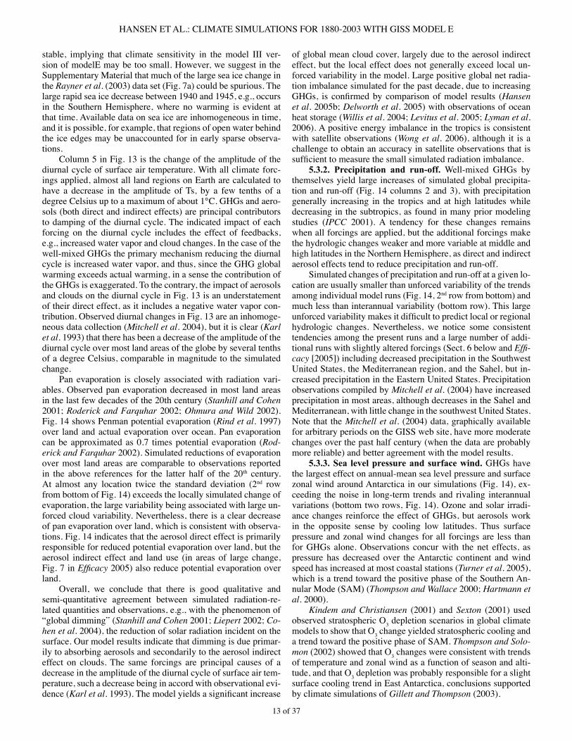
�3 of 37


stable, implying that climate sensitivity in the model III ver-sion of modelE may be too small. However, we suggest in the Supplementary Material that much of the large sea ice change in the Rayner et al. (2003) data set (Fig. 7a) could be spurious. The large rapid sea ice decrease between �940 and �945, e.g., occurs in the Southern Hemisphere, where no warming is evident at that time. Available data on sea ice are inhomogeneous in time, and it is possible, for example, that regions of open water behind the ice edges may be unaccounted for in early sparse observa-tions. Column 5 in Fig. �3 is the change of the amplitude of the diurnal cycle of surface air temperature. With all climate forc-ings applied, almost all land regions on Earth are calculated to have a decrease in the amplitude of Ts, by a few tenths of a degree Celsius up to a maximum of about �°C. GHGs and aero-sols (both direct and indirect effects) are principal contributors to damping of the diurnal cycle. The indicated impact of each forcing on the diurnal cycle includes the effect of feedbacks, e.g., increased water vapor and cloud changes. In the case of the well-mixed GHGs the primary mechanism reducing the diurnal cycle is increased water vapor, and thus, since the GHG global warming exceeds actual warming, in a sense the contribution of the GHGs is exaggerated. To the contrary, the impact of aerosols and clouds on the diurnal cycle in Fig. �3 is an understatement of their direct effect, as it includes a negative water vapor con-tribution. Observed diurnal changes in Fig. �3 are an inhomoge-neous data collection (Mitchell et al. 2004), but it is clear (Karl et al. �993) that there has been a decrease of the amplitude of the diurnal cycle over most land areas of the globe by several tenths of a degree Celsius, comparable in magnitude to the simulated change. Pan evaporation is closely associated with radiation vari-ables. Observed pan evaporation decreased in most land areas in the last few decades of the 20th century (Stanhill and Cohen 200�; Roderick and Farquhar 2002; Ohmura and Wild 2002). Fig. �4 shows Penman potential evaporation (Rind et al. �997) over land and actual evaporation over ocean. Pan evaporation can be approximated as 0.7 times potential evaporation (Rod-erick and Farquhar 2002). Simulated reductions of evaporation over most land areas are comparable to observations reported in the above references for the latter half of the 20th century. At almost any location twice the standard deviation (2nd row from bottom of Fig. �4) exceeds the locally simulated change of evaporation, the large variability being associated with large un-forced cloud variability. Nevertheless, there is a clear decrease of pan evaporation over land, which is consistent with observa-tions. Fig. �4 indicates that the aerosol direct effect is primarily responsible for reduced potential evaporation over land, but the aerosol indirect effect and land use (in areas of large change, Fig. 7 in Efficacy 2005) also reduce potential evaporation over land. Overall, we conclude that there is good qualitative and semi-quantitative agreement between simulated radiation-re-lated quantities and observations, e.g., with the phenomenon of “global dimming” (Stanhill and Cohen 200�; Liepert 2002; Co-hen et al. 2004), the reduction of solar radiation incident on the surface. Our model results indicate that dimming is due primar-ily to absorbing aerosols and secondarily to the aerosol indirect effect on clouds. The same forcings are principal causes of a decrease in the amplitude of the diurnal cycle of surface air tem-perature, such a decrease being in accord with observational evi-dence (Karl et al.1993).Themodelyieldsasignificantincrease

of global mean cloud cover, largely due to the aerosol indirect effect, but the local effect does not generally exceed local un-forced variability in the model. Large positive global net radia-tion imbalance simulated for the past decade, due to increasing GHGs, is confirmedby comparisonofmodel results (Hansen et al. 2005b; Delworth et al. 2005) with observations of ocean heat storage (Willis et al. 2004; Levitus et al. 2005; Lyman et al. 2006). A positive energy imbalance in the tropics is consistent with satellite observations (Wong et al. 2006), although it is a challenge to obtain an accuracy in satellite observations that is sufficienttomeasurethesmallsimulatedradiationimbalance. 5.3.2. Precipitation and run-off. Well-mixed GHGs by themselves yield large increases of simulated global precipita-tion and run-off (Fig. �4 columns 2 and 3), with precipitation generally increasing in the tropics and at high latitudes while decreasing in the subtropics, as found in many prior modeling studies (IPCC 200�). A tendency for these changes remains when all forcings are applied, but the additional forcings make the hydrologic changes weaker and more variable at middle and high latitudes in the Northern Hemisphere, as direct and indirect aerosol effects tend to reduce precipitation and run-off. Simulated changes of precipitation and run-off at a given lo-cation are usually smaller than unforced variability of the trends among individual model runs (Fig. �4, 2nd row from bottom) and much less than interannual variability (bottom row). This large unforcedvariabilitymakesitdifficulttopredictlocalorregionalhydrologic changes. Nevertheless, we notice some consistent tendencies among the present runs and a large number of addi-tional runs with slightly altered forcings (Sect. 6 below and Effi-cacy [2005]) including decreased precipitation in the Southwest United States, the Mediterranean region, and the Sahel, but in-creased precipitation in the Eastern United States. Precipitation observations compiled by Mitchell et al. (2004) have increased precipitation in most areas, although decreases in the Sahel and Mediterranean, with little change in the southwest United States. Note that the Mitchell et al. (2004) data, graphically available for arbitrary periods on the GISS web site, have more moderate changes over the past half century (when the data are probably more reliable) and better agreement with the model results. 5.3.3. Sea level pressure and surface wind. GHGs have the largest effect on annual-mean sea level pressure and surface zonal wind around Antarctica in our simulations (Fig. �4), ex-ceeding the noise in long-term trends and rivaling interannual variations (bottom two rows, Fig. �4). Ozone and solar irradi-ance changes reinforce the effect of GHGs, but aerosols work in the opposite sense by cooling low latitudes. Thus surface pressure and zonal wind changes for all forcings are less than for GHGs alone. Observations concur with the net effects, as pressure has decreased over the Antarctic continent and wind speed has increased at most coastal stations (Turner et al. 2005), which is a trend toward the positive phase of the Southern An-nular Mode (SAM) (Thompson and Wallace 2000; Hartmann et al. 2000). Kindem and Christiansen (200�) and Sexton (200�) used observed stratospheric O3 depletion scenarios in global climate models to show that O3 change yielded stratospheric cooling and a trend toward the positive phase of SAM. Thompson and Solo-mon (2002) showed that O3 changes were consistent with trends of temperature and zonal wind as a function of season and alti-tude, and that O3 depletion was probably responsible for a slight surface cooling trend in East Antarctica, conclusions supported by climate simulations of Gillett and Thompson (2003).

�4 of 37


Fyfe et al. (�999) and Kushner et al. (200�) found that well-mixed GHGs also induce a positive response of the SAM in their models, as upper tropospheric warming and lower stratospheric cooling strengthen the polar vortex in all seasons. This effect is enhanced by minimal warming in the deep-mixing circum-Ant-arctic Southern Ocean during the transient climate phase. Cai et al.(2003)findthatstabilizingtheGHGamountwouldweakenthe SAM, as the high latitude surface warms and reduces the zonal temperature gradient that drives the subpolar jet stream. Shindell and Schmidt (2004), with a version of the GISS model that includes gravity wave drag and a higher model top, findcomparablecontributionsofO3 and GHGs to surface change, with O3 dominating above the middle troposphere. The larger response to GHGs in our present model is likely a tropospheric effect, as we obtain large low-latitude upper-tropospheric warm-ing (Figs. ��a and �2), consistent with larger-than-observed sur-facewarminginthetropicalPacificOcean(overmostperiods,albeit not over �950-2003, Fig. 9). The larger-than-observed tropicalPacificwarminganduppertroposphericwarminginthesatellite era disappear when we use observed SSTs, as noted in Sect.5.1.1andTable2.GiventhelargefluctuationsofobservedtropicalPacificwarming(Fig.9),wesuggest that thediscrep-ancy between our ensemble mean result and the real world’s single realization in the satellite period (�979-2003), including surfacecoolingoftheAntarcticcontinent,couldbeareflectionofrealworldvariabilityratherthanamodelflaw.Indeed,despitethe lack of ENSO-like variability in the present model, some ensemble members have cooling over East Antarctica in �979-2003. Quantitative analysis requires a version of the model with more realistic tropical variability. Observed warming in recent decades (Fig. 9) and warming simulated by a large IPCC ensemble of many climate models in response to increasing GHGs (Carril et al. 2005) is concentrat-ed in the Amundson Sea-Antarctic Peninsula-Western Weddell Sea region, where recent acceleration of outlet glaciers has been noted (Thomas et al. 2004; Cook et al. 2004). Despite the coarse resolution of our model, the warming pattern that we obtain with “all forcings” is consistent with results of the ensemble of IPCC models (Carril et al. 2005). 5.3.4. Zonal mean quantities. Fig. �5 shows 5-run ensem-ble mean changes of zonal mean temperature, water vapor, zonal wind, and stream function produced by each forcing for �950-2003 and �979-2003 as a function of altitude and latitude. Con-trol run values of these quantities are shown in Efficacy (2005). The standard deviation for each quantity among changes in 54-year and 25-year segments of the control run are shown in the bottom row of Fig. �5. Conspicuous features in the zonal temperature response were discussed in connection with Figs. ��-�2. Water vapor changes, including stratospheric H2O,mainlyreflecttropospher-ic temperature change, except for forcings that directly alter stratospheric temperature. The large stratospheric H2O change due to CH4-oxidation warms the upper troposphere but barely affects the surface temperature. Note the large unforced variability of zonal winds at high latitudes. In the Northern Hemisphere only GHGs produce a re-sponse exceeding the variability among runs, and only on the 54-year period, not 25 years. A greater zonal-wind response is obtained in the Southern Hemisphere for GHG and O3 forcings, but the effect at the surface exceeds unforced variability only for GHGs on the longer time scale. The salient change of the meridional stream function caused

by “all forcings” is a strengthening of the overturning Brewer-Dobson circulation in the stratosphere. However, response of the Hadley circulation in the lower troposphere is the opposite, i.e., a weakening. These changes are due mainly to the well-mixed GHGs. Knutson and Manabe (�995) and Held and Soden (2006) show that weakening of mean overturning in the lower tropo-sphere, including the Walker circulation, is due to the increasing proportionofverticalenergyfluxcarriedbymoistconvectionas global warming increases. Changes of the stream function for different forcings are more systematic and apparent when viewed for individual seasons as in Efficacy (2005), where it is shown that stream function changes are approximately propor-tional to the effective forcing Fe and in the opposite sense for positive and negative Fe.5.4. Alternative Aerosol Forcings A primary discrepancy between our simulated global tem-perature change and observations is the small modeled warming at middle latitudes in the Northern Hemisphere. A likely cause ofthisdeficientwarmingisthelargeincreaseofaerosolopticaldepth in our model between �880 and 2003. Causes of large aerosol optical depth in our model include (see Sect. 3.2.�): (�) Sulfate optical depths are from results of Koch (200�) available at the time our “IPCC” runs were initiated. More re-cent results of Koch (personal communication), based on new emissiondata andmore efficient removal including the effectof heterogeneous chemical reactions of sulfate and mineral dust (Bauer and Koch 2005), reduce the sulfate optical depth about 50%. (2) Our aerosol distributions were calculated at coarse tem-poral intervals (Sect. 3.2), the most recent date being �990, after which aerosol amount is constant (except nitrate, which increas-es in proportion to global population). Thus we do not capture post-�990 aerosol decreases in Europe and the United States (see Sect. 5.�), nor aerosol increases in developing countries. It would be useful to rerun some of our experiments with the best current estimates of global aerosol distributions. How-ever,severalsignificantimprovementsofouroceanandatmo-sphere models are also now practical. Thus we plan to repeat the transient climate change experiments with the next documented version of our climate model using the best data then avail-able for aerosols and other transient climate forcings. Here we only make two aerosol sensitivity runs with the present climate model, to provide an indication of how changes in the assumed aerosols affect the simulated climate. In the aerosol “½ Sulfates” experiment the sulfate changes were reduced by 50%, which also reduced the (negative) AIE by about �8%. In the “½ Sulfates + 2x[Biomass Burning]” ex-periment the temporal change of BC and OC aerosols from bio-mass burning was doubled, in addition to the reduction of fossil fuel sulfates. Fig. �6 summarizes the impact of these alternative aerosol histories on the simulated temperature change, compar-ing the results with observations and the standard “all forcing” model runs. The reduction of sulfates, which changes the net aerosol �880-2003 global forcing from –�.37 W/m2 to –0.9� W/m2, in-creases global warming from 0.53 to 0.75°C for �880-2003 and from 0.40 to 0.53°C for �950-2003. Doubling of the biomass burning aerosol change has little further effect on global temper-ature (Fig. �6a) as the warming from added BC approximately cancels cooling from added OC. Both alternative aerosol distributions increase the warm-

�5 of 37


ing at middle latitudes in the Northern Hemisphere to a realistic level as a result of reduced reflective (sulfate) aerosol opticaldepth. Given the evidence that our standard aerosol amount was excessive, and does not include post-�990 changes, it is likely that aerosols are a principal factor that needs to be improved in the standard forcings. However, the present alternative distribu-tions should only be viewed as sensitivity studies, as acceptable alternativesneedtobeobtainedfromfirstprinciplesusingim-proved aerosol observations and modeling. There is notable polar amplification of simulated surfacewarming in the Northern Hemisphere over the past half century and longer periods, in the cases with aerosol amount reduced to a level that yields realistic mid-latitude warming (Fig. �6c). However, observed polar amplification fluctuates greatly de-pendingontheperiodconsidered,whichisareflectionofhow‘noisy’ high latitude temperature is (Sorteberg et al. 2005; Bitz and Goosse 2006. ThegraybandinFig.16cisdefinedbythe1σvariationinthe 5-member ensemble of runs for our standard case with all forcings. As would be expected, for some periods and latitudes theobservationsfalloutside the1σrange,althoughalmostallcasesarewithin2σ.Notethegreatvariabilityofobservedhighlatitude temperature change depending on the period consid-ered and the large unforced variability of the polar temperatures among model runs. Given that the real world represents a single realization, the large unforced variability at high latitudes indi-cates that observed climate changes at high latitudes should be interpreted with caution.6. Summary: Model and Data Limitations and Potential We summarize model limitations and capabilities (Sect. 6.�) andbrieflydiscuss(Sect.6.2)why,despitethemodellimitations,extension of model runs into the future can provide meaningful results. In Sect. 6.3 we summarize lessons learned that may be helpful for future climate simulations.6.1. Global Climate Change: 1880-2003 Our climate model, driven by all of the estimated forcings, simulates observed global mean temperature change over the period1880-2003reasonablywell.Theresultsfitobservationsbetter if tropospheric aerosol change is smaller over Europe than it is in our standard ‘all forcing’ run. There are independent rea-sons to believe that a reduced aerosol change there is more real-istic, as discussed in Sect. 5.4. The match of simulated and observed global temperature curves is not an indication that knowledge of climate sensitiv-ity and the mechanisms causing climate change is as accurate assuggestedbythatfit.Anequallygoodmatchtoobservationsprobably could be obtained from a model with larger sensitivity (than 2.9°C for doubled CO2) and smaller net forcing, or a model with smaller sensitivity and larger forcing. Indeed, although de-tailed temporal and spatial patterns of climate change, in prin-ciple, may allow extraction of inferences about both climate sensitivity and forcings, in practice the large unforced variabil-ity of climate, uncertainties in observed climate change, poor knowledge of aerosol forcings, and imprecision in the model-generatedresponsetoforcingsmakeitdifficulttoplaceusefulquantitative limits on climate sensitivity from observed climate change of the past century. On the other hand, paleoclimate evidence of climate change between periods with well-known boundary conditions (forc-ings) yields a climate sensitivity 3±�°C for doubled CO2 (Han-sen et al. �993), so our model sensitivity of 2.9°C for doubled

CO2 is reasonable. The realistic response of this model to the accurately known short-term forcing by Pinatubo volcanic aero-sols and the realistic rate of simulated global warming in the past 3-4 decades, when greenhouse gases increased so rapidly that they dominated over other estimated forcings (Fig. 5), suggest that approximate agreement between observed and simulated global temperature is not fortuitous. The largest discrepancy in simulated �880-2003 surface temperature change, other than deficient warming in Eurasia,iswarmingofthetropicalPacificOceanthatexceedsobserva-tions (Fig. 9). Cane et al. (�997) suggest that reduced warming in that region may occur with global warming due to increased frequency or intensity of La Ninas, but among all models there is a slight tendency toward increased El Ninos with global warm-ing (Collins et al. 2005). Our present model would not be able to capture a change in ENSO variability, whether forced or un-forced. However, note that the existence of a discrepancy in PacificOceanwarmingdependsontheperiodconsidered.Forexample, ourmodeled tropical Pacificwarming is larger thanobserved for �880-2003, but not for �950-2003 (Figs. 9 and �6c). We conclude that observed variability in tropical surface temperature trends is a strong function of ENSO variability, and the differences between observations and simulations in this re-gion may be due simply to unforced variability. The greatest apparent discrepancy with observations of temperature change versus altitude is the large simulated warm-ing in the tropical upper troposphere. On the 50-year time scale there is no clear evidence that modeled upper tropospheric warming exceeds observations, given increasing evidence that deficientwarmingthereinradiosonderecordsmaybeafigmentof inhomogeneities in the radiosonde data sources (Sherwood et al. 2005; Free and Seidel 2005; Santer et al. 2005b; Karl et al. 2006). However, on shorter time scales our modeled upper tropospheric warming trend is excessive, as shown most con-vincingly by MSU T/S data for �987-2003. But this excessive upper tropospheric warming disappears when we use ocean A (observed SSTs) instead of the fully coupled atmosphere-ocean model (complete ocean A results are available at data.giss.nasa.gov/modelE/transient). Thus the excessive upper tropospheric warmingisareflectionoflargerthanobservedwarmingofthetropicalPacificOceaninthecoupledmodel.Realworldtrendstoward La Nina conditions for �987-2003, toward El Nino con-ditions for �950-2003, and slightly toward La Nina conditions for �880-2003 (Fig. 9) are within the range of Southern Oscilla-tion variability. There is no reason to expect our model to cap-turethisspecificENSOvariability,andthereisnoinconsistencybetween upper tropospheric and surface temperature changes. Thusweanticipatethatmagnifiedwarminginthetropicaluppertroposphere will become apparent as the tropical ocean contin-ues to warm in response to increasing GHGs. In summary, simulated climate change for the past century does not agree in detail with observations, nor would it be ex-pected to agree, given unforced climate variability, uncertain-ty in climate forcings, and current model limitations. But in a broad sense our climate model does a credible job of simulating observed global temperature change in response to short time-scale (volcanic aerosol) as well as century time-scale forcings. Thismodelcapabilityprovidessufficientreasontoexaminethemodel for information about large-scale regional climate effects of practical importance and to extend the climate simulations to investigate potential global consequences of alternative climate forcing scenarios.

�6 of 37


6.2. Extended Simulations Given the large uncertainty in the net climate forcing during the past century (Sect. 3.4), due mainly to aerosols, it may be questioned whether useful accuracy can be achieved in simula-tions of the future. However, GHG climate forcing is expected to be dominant over aerosol forcing in the future; indeed, it seems likely that at least a moderate decrease of aerosol amount will occur (Andreae et al. 2005; Smith et al. 2005). Therefore, givenaspecifiedGHGscenario,withlargeincreasesofGHGsas projected by IPCC (200�), the relative uncertainty in the net forcing is reasonably small. Thus, continuations of some of our present �880-2003 simulationsintothefutureseemjustified.Wehaveextendedthe�880-2003 “all forcing” simulations of this paper to 2�00, and inafewcasesto2300usingfixed2003forcings,severalIPCCGHG scenarios, and the “alternative” and “2°C” scenarios of Hansen and Sato (2004). These extended simulations are de-scribed in Dangerous (2006).6.3. Lessons Learned Our control run had negligible stratospheric aerosols, rep-resenting only “background” conditions far removed from the injection of aerosols by large volcanoes. If volcanic aerosols are to be included as a forcing in experiment runs, the use of ocean initial conditions from a control run without volcanic aerosols yields misleading results, especially for ocean heat storage. In Supplement Sect. S2 we suggest that inclusion of a mean aerosolamountinthecontrolrunsignificantlyimprovesrealismof results. We now include in our control runs a mean strato-sphericaerosolopticalthicknessτ=0.0125at0.55μmwave-length, which is the �850-2000 mean value of the Sato et al. (�993) aerosol climatology. Other researchers may wish to con-sider including this mean stratospheric aerosol amount in their control runs. Other “lessons learned” concern methods to minimize the effectofmodeldrift(S3)andtheeffectofmixeddefinitionsofsurface air temperature (S3). We also describe minor errors in ozone forcing (S4) and the forcing due to black carbon deposi-tiononsnow(S5).TheefficacyoftheBCsnowalbedoeffectisfound to be 2.7 after the programming error is corrected, rather than �.7 that was reported in Efficacy (2005), where the same programming error was included.

Acknowledgments. Data that we use for recent greenhouse gas amounts are from the NOAA Earth System Research Laboratory, Global Moni-toring Division, where we are particularly indebted to Ed Dlugokencky, Steve Montzka, and Jim Elkins for up-to-date data. We thank Ellen Baum, Tom Boden, Curt Covey, Oleg Dubovik, Hans Gilgen, Danny Harvey, Brent Holben, Phil Jones, John Lanzante, Judith Lean, Forrest Mims, Bill Randel, Eric Rignot for data and helpful suggestions, and Darnell Cain for technical assistance. Research support from Hal Har-vey of the Hewlett Foundation, Gerry Lenfest, and NASA Earth Sci-ence Research Division managers Jack Kaye, Don Anderson, Waleed Abdalati, Phil DeCola, Tsengdar Lee, and Eric Lindstrom is gratefully acknowledged.

ReferencesAndreae MO, Jones CD, Cox PM (2005) Strong present-day aerosol

cooling implies a hot future. Nature 435:��87—��90.Andreae MO, Gelencser A (2006) Black carbon or brown carbon? The

nature of light-absorbing carbonaceous aerosols. Atmos Chem Phys 6:3�3�—3�48.

Baldwin MP, Dunkerton TJ (2005) The solar cycle and stratosphere-troposphere dynamical coupling. J Atmos Sol Terr Phys 67:7�—82.

Bauer, SE, D Koch (2005) Impact of heterogeneous sulfate formation at mineral dust surfaces on aerosol loads and radiative forcing in the Goddard Institute for Space Studies general circulation model. J Geo-phys Res ��0:D�7202. DOI �0.�029/2005JD005870.

Betts RA (200�) Biogeophysical impacts of land use on present-day climate: Near-surface temperature and radiative forcing. Atmos Sci Lett 2:39—5�.

Bitz CM, Goosse H (2006) Transient polar amplification in twenti-eth century observations and climate simulations. Geophys Res Lett (submitted). Accessed 24 Jan 2007 at http://www.atmos.washington.edu/~bitz/bitz_goosse.pdf.

Bleck R (2002) An oceanic general circulation model framed in hybrid isopycnic-Cartesian coordinates. Ocean Model 4:55—88.

Bohren CF (�986) Applicability of effective-medium theories to prob-lems of scattering and absorption by nonhomogeneous atmospheric particles. J Atmos Sci 43:468—475.

Bond TC, Streets DG, Yarber KF, Nelson SM, Woo JH, Klimont Z (2004) A technology-based global inventory of black and organic car-bon emissions from combustion. J Geophys Res �09:D�4203. DOI �0.�029/2003JD003697.

Cai W, Whetton PH, Karoly DJ (2003). The response of the Antarc-tic Oscillation to increasing and stabilized atmospheric CO2. J Clim �6:�525—�538.

Cane MA, Clement AC, Kaplan A, Kushnir Y, Pozdnyakov D, Seager R, Zebiak SE, Murtugudde R (�997) Twentieth century sea surface temperature trends. Science 275:957—960.

Carril AF, Menendez CG, Navarra A (2005) Climate response associ-ated with the Southern Annular Mode in the surroundings of Antarctic Peninsula: A multimodel ensemble analysis. Geophys Res Lett 32:L�67�3. DOI �0.�029/2005GL02358�.

Chapin FS et al (2005) Role of land-surface changes in Arctic summer warming. Science 3�0:657—660.

Che HZ, Shi GY, Zhang XY, Arimoto R, Zhao JQ, Xu L, Wang B, Chen ZH (2005) Analysis of 40 years of solar radiation data from China, �96�-2000. Geophys Res Lett 32:L06803. DOI �0.�029/2004GL022322.

Christy JR, Spencer RW, Braswell WD (2000). MSU tropospheric tem-peratures: Data set construction and radiosonde comparisons. J Atmos Oceanic Technol �7:��53—��70.

Chylek P, Videen G, Ngo D, Pinnick RG, Klett JD (�995) Effect of black carbon on the optical properties and climate forcing of sulfate aerosols. J Geophys Res �00:�6325—�6332.

Clarke AD, Noone KJ (�985) Soot in the Arctic snowpack: a cause for perturbations in radiative transfer. Atmos Environ �9:2045—2053.

Cohen S, Liepert B, Stanhill G (2004) Global dimming comes of age. EOS Trans Amer Geophys Union 85:362.

Collins M et al (2005) El Nino or La Nina-like climate change? Clim Dyn 24:89—�04.

Collins WD et al (2006) Radiative forcing by well-mixed greenhouse gases: Estimates from climate models in the IPCC AR4. J Geophys Res ��:D�43�7. DOI �0.�029/2005JD0067�3.

Cook ER, Woodhouse C, Eakin CM, Meko DM, Stahle DW (2004) Long-term aridity changes in the western United States. Science 306:�0�5—�0�8.

Del Genio AD, Kovari W, Yao MS, Jonas J (2005) Cumulus microphys-ics and climate sensitivity. J Clim �8:2376—2387.

Delworth TL, Ramaswamy V, Stenchikov GL (2005) The impact of aero-sols on simulated ocean temperature and heat content in the 20th cen-tury. Geophys Res Lett 32:L24709. DOI �0.�029/2005GL024457.

Dubovik O, Holben B, Eck TF, Smirnov A, Kaufman YJ, King MD, Tanré D, Slutsker I (2002) Variability of absorption and optical prop-erties of key aerosol types observed in world-wide locations, J Atmos Sci 59:590—608.

Eddy J (�976) The Maunder minimum. Science �92:��89—�202.Fleming EL, Jackman CH, Stolarski RS, Considine DB (�999) Simu-

https://www.researchgate.net/publication/null?el=1_x_8&enrichId=rgreq-265bebb59cdcfa116eb1cefaf2466d2c-XXX&enrichSource=Y292ZXJQYWdlOzIzNzA4ODM0OTtBUzoxMDIyMzE3ODUzNDUwMjlAMTQwMTM4NTM2NTM5MA==

�7 of 37


lation of stratospheric tracers using an improved empirically based two-dimensional model transport formulation. J Geophys Res �04:239��—23934.

Foley JA et al (2005) Global consequences of land use. Science 309:570—574.

Forest CE, Stone PH, Sokolov AP (2006) Estimated PDFs of climate system properties including natural and anthropogenic forcings. Geo-phys Res Lett 33:L0�705. DOI �0.�029/2005GL023977.

Free M, Seidel DJ (2005) Causes of differing temperature trends in radiosonde upper air data sets. J Geophys Res ��0:D07�0�. DOI �0.�029/2004JD00548�.

Fu Q, Johanson CM (2005) Satellite-derived vertical dependence of tropical tropospheric temperature trends. Geophys Res Lett 32:L�0703. DOI �0.�029/2004GL022266.

Fyfe JC, Boer GJ, Flato GM (�999) The Arctic and Antarctic Oscilla-tions and their projected changes under global warming. Geophys Res Lett 26:�60�—�604.

Gauss M et al (2003) Radiative forcing in the 2�st century due to ozone changes in the troposphere and lower stratosphere. J Geophys Res �08(D9):4292. DOI �0.�029/2002JD002624.

Gent PR, Willebrand J, McDougall TJ, McWilliams JC (�995) Param-eterizing eddy-induced tracer transports in ocean circulation models. J Phys Oceanogr 25:463—474.

Gilgen H, Wild M, Ohmura A (�998) Means and trends of shortwave irradiance at the surface estimated from global energy balance archive data. J Clim ��:2042—206�.

Gillett NP, Thompson DWJ (2003) Simulation of recent Southern Hemisphere climate change. Science 302:273—275.

Grenfell TC, Light B, Sturm B (2002) Spatial distribution and radiative effects of soot in the snow and sea ice during the SHEBA experiment. J Geophys Res �07(C�0):803�. �0.�029/2000JC0004�4.

GriffiesSM(1998)TheGent-McWilliamsskewflux.JPhysOceanogr28:83�—84�.

Haigh JD (�994) The role of stratospheric ozone in modulating the so-lar radiative forcing of climate. Nature 370:544—546.

Hansen J, Lacis A, Rind D, Russell G, Stone P, Fung I, Ruedy R, Lerner J (�984) Climate sensitivity: Analysis of feedback mechanisms. In: Hansen JE, Takahashi T (eds) Climate Processes and Climate Sen-sitivity, Geophys Monograph Series No. 29. American Geophysical Union, Washington, DC, pp �30—�63.

Hansen J, Lacis A, Ruedy R, Sato M, Wilson H (�993) How sensitive is the world’s climate? Natl Geogr Res Explor 9:�42—�58.

Hansen J et al (�997a) Forcings and chaos in interannual to decadal climate change. J Geophys Res �02:25679—25720.

Hansen J, Sato M, Ruedy R (�997b) Radiative forcing and climate re-sponse. J Geophys Res �02:683�—6864

Hansen JE, Sato M, Lacis A, Ruedy R, Tegen I, Matthews E (�998a) Climate forcings in the Industrial Era. Proc Natl Acad Sci 95:�2753—�2758.

Hansen, JE, Sato M, Ruedy R, Lacis A, Glascoe J (�998b). Global cli-mate data and model: A reconciliation. Science 28�:930—932.

Hansen J, Ruedy R, Sato M, Imhoff M, Lawrence W, Easterling D, Peterson T, Karl T (200�) A closer look at United States and global surface temperature change. J Geophys Res �06:23947—23963.

Hansen J et al (2002) Climate forcings in Goddard Institute for Space Studies SI2000 simulations. J Geophys Res �07(D�8):4347. DOI �0.�029/200�JD00��43.

Hansen J, Bond T, Cairns B, Gaeggler H, Liepert B, Novakov T, Schich-tel B (2004) Carbonaceous aerosols in the Industrial Era. EOS Trans Amer Geophys Union 85:24�, 244.

Hansen J, Nazarenko L (2004). Soot climate forcing via snow and ice albedos. Proc Natl Acad Sci �0�:423—428.

Hansen J, Sato M (2004). Greenhouse gas growth rates. Proc Natl Acad Sci �0�:�6�09—�6��4.

HansenJetal(2005a)Efficacyofclimateforcings.JGeophysRes110:D�8�04. DOI �0.�029/2005JD005776.

HansenJetal(2005b)Earth’senergyimbalance:confirmationandim-plications. Science 308:�43�—�435.

Hansen J, Sato M, Ruedy R, Lo K, Lea DW, Medina-Elizade M (2006a) Global temperature change. PNAS �03:�4288-�4293.

Hansen J et al (2006b) Dangerous human-made interference with cli-mate: A GISS modelE study. Atmos Chem Phys Discuss 6:�2549—�26�0.

Hartmann DL, Wallace JM, Limpasuvan V, Thompson DWJ, Holton JR (2000) Can ozone depletion and global warming interact to produce rapid climate change? Proc Natl Acad Sci 97:�4�2—�4�7.

Harvey LDD (2000) Global Warming: The Hard Science. Prentice Hall, 336 pp.

Harvey LDD, Kaufmann RK (2002) Simultaneously constraining cli-mate sensitivity and aerosol radiative forcing. J Clim �5:2837-286�.

Harvey LDD (2004) Characterizing the annual-mean climatic effect of anthropogenic CO2 and aerosol emissions in eight coupled atmo-sphere-ocean GCMs. Clim Dyn 23:569-599.

Held IM, Soden BJ (2006) Robust responses of the hydrological cycle to global warming. J Clim �9:5686—5699.

Hoffert MI, Covey C (�992) Deriving global climate sensitivity from paleoclimate reconstructions. Nature 360:573—576.

Holben BN et al (200�) An emerging ground-based aerosol climatology: Aerosol optical depth from AERONET. J Geophys Res �06:�2067—�2098.

Hoyt D, Schatten K (�993) A discussion of plausible solar irradiance variations. J Geophys Res 98:�8895—�8906.

Intergovernmental Panel on Climate Change (IPCC) (�996) Climate Change �995: The Science of Climate Change. Houghton JT, Mei-ra Filho LG, Callender BA, Harris, N, Kattenberg, Maskell K (eds) Cambridge University Press, Cambridge, UK.

Intergovernmental Panel on Climate Change (IPCC) (200�) Climate Change2001:TheScientificBasis.HoughtonJT,DingY,GriggsDJ,Noguer M, van der Linden PJ, Dai X, Maskell K, Johnson CA (eds) Cambridge University Press, Cambridge, UK.

Johannessen OM et al (2004) Arctic climate change: Observed and modeled temperature and sea-ice variability. Tellus 56A:328—34�.

Jones PD, New M, Parker DF, Martin S, Rigor LG (�999) Surface air temperature and its changes over the past �50 years. Rev Geophys 37:�73—�99.

Kalnay E et al (�996) The NCEP/NCAR 40-year reanalysis project. Bull Amer Meteorol Soc 77:437—47�.

Karl TR, Jones PD, Knight RW, Kukla G, Plummer N, Razyiuvayev V, Gallo KP, Lindseay J, Charlson RJ, Peterson TC (�993) A new perspective on recent global warming – asymmetric trends of daily maximum and minimum temperature. Bull Amer Meteorol Soc 74:�007—�023.

Karl TR, Hassol SJ, Miller CD, Murray WL (eds) (2006) Temperature trends in the lower atmosphere: Steps for understanding and recon-ciling differences – Synthesis and assessment product �.�. Climate Change Science Program and the Subcommittee on Global Change Research, Washington DC. Accessed 24 Jan 2007 at http://www.cli-matescience.gov/Library/sap/sap1-1/finalreport/.

Kim DH, Nakashiki N, Yoshida Y, Maruyama K, Bryan FO (2005) Regional cooling in the South Pacific sector of the SouthernOcean due to global warming. Geophys Res Lett 32:L�9607. DOI �0.�029/2004GL023708.

Kindem, I.T, B Christiansen (200�) Tropospheric response to strato-spheric ozone loss. Geophys Res Lett 28:�547—�550.

Kirchstetter, TW, T Novakov, PH Hobbs (2004) Evidence that the spec-tral dependence of light absorption by aerosols is affected by organic carbon. J Geophys Res �09:D2�208. DOI �0/�029/2004JD004999.

Knutson TR, Manabe S (�995) Time-mean response over the Tropi-calPacifictoincreasedCO2 in a coupled ocean-atmosphere model. J Clim 8:2�8�—2�99.

Koch D (200�) Transport and direct radiative forcing of carbonaceous and sulfate aerosols in the GISS GCM. J Geophys Res �06:203��—

https://www.researchgate.net/publication/233614478_Characterizing_the_annual-mean_climatic_effect_of_anthropogenic_CO2_and_aerosol_emissions_in_eight_coupled_atmosphere-ocean_GCMs?el=1_x_8&enrichId=rgreq-265bebb59cdcfa116eb1cefaf2466d2c-XXX&enrichSource=Y292ZXJQYWdlOzIzNzA4ODM0OTtBUzoxMDIyMzE3ODUzNDUwMjlAMTQwMTM4NTM2NTM5MA==

https://www.researchgate.net/publication/255027572_Time-Mean_Response_over_the_Tropical_Pacific_to_Increased_C0_2_in_a_Coupled_Ocean-Atmosphere_Model?el=1_x_8&enrichId=rgreq-265bebb59cdcfa116eb1cefaf2466d2c-XXX&enrichSource=Y292ZXJQYWdlOzIzNzA4ODM0OTtBUzoxMDIyMzE3ODUzNDUwMjlAMTQwMTM4NTM2NTM5MA==

�8 of 37


20332.Koch D, Hansen J (2005) Distant origins of Arctic black carbon: A

Goddard Institute for Space Studies ModelE experiment. J Geophys Res ��0:D04204. DOI �0.�029/2004JD005296.

Kushner PJ, Held IM, Delworth TL (200�) Southern Hemisphere at-mospheric circulation response to global warming, J Clim �4:2238—2249.

Lacis A, Hansen J, Sato M (�992) Climate forcing by stratospheric aerosols. Geophys Res Lett �9:�607-�6�0.

Large WG, McWilliams JC, Doney SC (�994) Oceanic vertical mixing: a review and a model with a nonlocal boundary layer parameteriza-tion. Rev Geophys 32:363—403.

Lean J (2000) Evolution of the sun’s spectral irradiance since the Maun-der Minimum. Geophys Res Lett 27:2425—2428.

Lean JL, Wang YM, Sheeley NR (2002) The effect of increasing solar activity on the Sun’s total and openmagnetic flux duringmultiplecycles: implications for solar forcing of climate. Geophys Res Lett 29(24):2224. DOI �0.�029/2002GL0�5880.

Lohmann U, Feichter J (2005) Global indirect aerosol effects: A review. Atmos Chem Phys 5:7�5—737.

Levitus S, Anatov JI, Boyer TP (2005) Warming of the world ocean, �955-2003. Geophys Res Lett 322:L02604. DOI �0.�029/2004GL02�592.

Liao H, Seinfeld JH, Adams PJ, Mickley LJ (2004) Global radia-tive forcing of coupled tropospheric ozone and aerosols in a uni-fied general circulation model. J Geophys Res 109:D16207. DOI�0.�029/2003JD004456.

Liepert BG (2002) Observed reductions of surface solar radiation at sites in the United States and worldwide from �96� to �990. Geophys Res Lett 29(�0):�42�. DOI �0.�029/2002GL0�49�0.

Liepert BG, Tegen I (2002) Multidecadal solar radiation trends in the United States and Germany and direct tropospheric aerosol forcing. J Geophys Res �07(D�2):4�53. DOI �0.�029/200�JD000760.

Liousse, C, Penner JE, Chuang, C, Walton, JJ, Eddleman, H, Cachier, H (�996) A global thre-dimensional model study of carbonaceous aero-sols. J Geophys Res �0�:�94��—�9432.

Liu J, Schmidt GA, Martinson DG, Rind D, Russell GL, Yuan X (2003) Sensitivity of sea ice to physical parameterizations in the GISS global climate model. J Geophys Res �08(C2):3053. DOI �0.�029/200�JC00��67.

Lyman JM, Willis JK, Gregory GC (2006) Recent cooling of the upper ocean. Geophys Res Lett 33:L�8604. DOI �0.�029/2006GL027033.

Manabe S, Stouffer RJ, Spelman MJ, Bryan K (�99�) Transient re-sponses of a coupled ocean-atmosphere model to gradual changes of atmospheric CO2, Part I: Annual mean response. J Clim 4:785—8�8.

Mears CA, Schabel M, Wentz FJ (2003) A reanalysis of the MSU Chan-nel 2 tropospheric temperature record. J Clim �6:3650—3664.

Mears CA, Wentz FJ (2005) The effect of diurnal correction on satellite-derived lower tropospheric temperature. Science 309:�548—�55�.

Menon S, Del Genio A (2006) Evaluating the impacts of carbonaceous aerosols on clouds and climate. In: Schlesinger ME et al (eds) Hu-man-Induced Climate Change: An Interdisciplinary Assessment. Cambridge Univ. Press, in press.

Miller RL, Schmidt GA, Shindell DT (2006) Forced annular variabil-ity in the 20th century Intergovernmental Panel on Climate Change Fourth Assessment Report models. J Geophys Res ��:D�8�0�. DOI �0.�029/2005JD006323.

Mishchenko MI, Cairns B, Hansen JE, Travis LD, Burg R, Kaufman YJ, Martins JV, Shettle EP (2004) Monitoring of aerosol forcing of climate from space: Analysis of measurement requirements. J Quant Spec Rad Trans 88:�49—�6�.

Mishchenko MI, Cairns B, Kopp G, Schueler CF, Fafaul BA, Hansen JE, Hooker RJ, Itchkawich T, Maring HB, Travis LD (2006) Precise and accurate monitoring of terrestrial aerosols and total solar irradi-ance: Introducing the Glory mission. Bull Amer Meteorol Soc (sub-mitted).

Mitchell TD, Carter TR, Jones PD, Hulme M, New M (2004) A com-

prehensive set of high-resolution grids of monthly climate for Eu-rope and the globe: the observed record (�90�-2000) and �6 scenarios (200�-2�00). Tyndall Working Paper 55. Tyndall Centre for Climate Change Research, Norwich and Oxford, UK. Accessed 24 Jan 2007 at http://www.tyndall.ac.uk/publications.

Montzka SA, Butler JH, Elkins JW, Thompson TM, Clarke AD, Lock LT (�999) Present and future trends in the atmospheric burden of ozone-depleting halogens. Nature 398:690—694.

Myhre G, Myhre A (2003) Uncertainties in radiative forcing due to sur-face albedo changes caused by land use changes. J Clim �6:�5��—�524.

Myhre G, Govaerts Y, Haywood JM, Berntsen TK, Lattanzio A (2005) Radiative effect of surface albedo change from biomass burning. Geophys Res Lett 32:L208�2. DOI �0.�029/2005GL022897.

Novakov T, Ramanathan V, Hansen JE, Kirchstetter TW, Sato M, Sinton JE, Sathaye JA (2003) Large historical changes of fos-sil-fuel black carbon aerosols. Geophys Res Lett 30(6):�324. DOI �0.�029/2002GL0�6345.

Novakov T, Menon S, Kirchstetter TW, Koch D, Hansen JE (2005) Aerosol organic carbon to black carbon ratios: analysis of published data and implications for climate forcing. J Geophys Res ��0:D2�205. DOI �0.�029/2005JD005977.

Ohmura A, Wild M (2002) Is the hydrological cycle accelerating. Sci-ence 298:�345—�346.

Palmer KF, Williams D (�975) Optical constants of sulfuric acid. Appl Opt �4:208—2�9.

Parker DE, Gordon M, Cullum DPN, Sexton DMH, Folland CK, Rayner N (�997) A new global gridded radiosonde temperature database and recent temperature trends. Geophys Res Lett 24:�499—�502.

Penner JE, Quaas J, Storelvmo T, Takemura T, Boucher O, Guo H, Kirkevåg A, Kristjánsson JE, Seland Ø (2006) Model intercompari-son of indirect aerosol effects. Atmos Chem Phys 6:339�—3405.

Preunkert S, Legrand M, Wagenbach D (200�) Sulfate trends in a col du Dome (French alps) ice core: A record of anthropogenic sulfate levels in the European midtroposphere over the twentieth century. J Geophys Res �06:3�99�—32004.

QuaasJ,BoucherO(2005)Constrainingthefirstaerosolindirectradia-tive forcing in the LMDZ GCM using POLDER and MODIS satellite data. Geophys Res Lett 32:L�78�4. DOI �0.�029/2005GL023850.

Ramankutty N, Foley JA (�999) Estimating historical changes in global land cover: croplands from �700 to �992. Global Biogeochem Cycles �3:997—�027.

Ramaswamy V et al (200�) Radiative forcing of climate change. Chap-ter6 in:Houghtonetal (eds)ClimateChange2001:TheScientificBasis. Cambridge University Press, Cambridge, UK, pp 349—4�6.

Randel WJ, Wu F (�999) A stratospheric ozone trends data set for glob-al modeling studies. Geophys Res Lett 26:3089—3092.

Rayner NA, Parker DE, Horton EB, Folland CK, Alexander LV, Rowell DP, Kent EC, Kaplan A (2003) Global analyses of SST, sea ice and night marine air temperatures since the late nineteenth century. J Geo-phys Res �08(D�4):4407. DOI �0.�029/2002JD002670.

Reichler T, Dameris M, Sausen R, Nodorp D (�996) A global climatol-ogy of the tropopause height based on ECMWF analyses. Institutsre-ports des Institut für Physik der Atmosphäre 57. Deutsches Zentrum für Luft- und Raumfahrt, Wessling, Germany.

Rind D, Rosenzweig C, Stieglitz M (�997) The role of moisture trans-port between ground and atmosphere in global change. Ann Rev En-ergy Environ 22:47—74.

Roderick ML, Farquhar GD (2002) The cause of decreased pan evapo-ration over the past 50 years. Science 298:�4�0—�4��.

Russell GL, Miller JR, Tsang LC (�985) Seasonal oceanic heat trans-ports computed from an atmospheric model. Dyn Atmos Oceans 9:253—27�.

Russell GL, Miller JR, Rind DH (�995) A coupled atmosphere-ocean model for transient climate change. Atmos Ocean 33:683—730.

Santer BD, Wehner MF, Wigley TML, Sausen R, Meehl GA, Taylor

https://www.researchgate.net/publication/230892158_Transient_Responses_of_a_Coupled_Ocean-Atmosphere_Model_to_Gradual_Changes_of_Atmospheric_CO2_Part_I_Annual_Mean_Response?el=1_x_8&enrichId=rgreq-265bebb59cdcfa116eb1cefaf2466d2c-XXX&enrichSource=Y292ZXJQYWdlOzIzNzA4ODM0OTtBUzoxMDIyMzE3ODUzNDUwMjlAMTQwMTM4NTM2NTM5MA==

�9 of 37


KE, Ammann C, Arblaster J, Washington WM, Boyle JS, Brugge-mann W (2003) Contributions of anthropogenic and natural forcing to recent tropopause height changes. Science 30�:479—483.

SanterBDet al (2005a)Amplificationof surface temperature trendsand variability in the tropical atmosphere. Science 309:�55�—�556.

Santer BD, Wigley TML, Taylor KE, Thorne PW, Wehner MF, Boyle JS, Collins W, Dixon KW, Doutriaux C, Gleckler PJ, Hansen JE, Karl TR, Klein SA, Lanzante JR, Mears C, Meehl GA, Ramaswamy V, Se-idel DJ, Wentz FJ (2005b) Modeled and observed lapse-rate changes in the deep tropics. Science 309:�55�—�556.

Sato M, Hansen J, McCormick MP, Pollack JP (�993) Stratospheric aerosol optical depths, �850-�990. J Geophys Res 98:22987—22994.

Sato M, Hansen J, Koch D, Lacis A, Ruedy R, Dubovik O, Holben B, Chin M, Novakov T (2003) Global atmospheric black carbon inferred from AERONET. Proc Natl Acad Sci �00:63�9—6324.

Schmidt GA et al (2006) Present day atmospheric simulations using GISS ModelE: Comparison to in-situ, satellite and reanalysis data. J Clim �9:�53—�92.

Schwikowski M, Brutsch S, Gaggeler HW, Schotterer U (�999) A high resolution air chemistry record from an Alpine ice core (Fiescherhorn glacier, Swiss Alps). J Geophys Res �04:�3709—�3720.

Sexton DMH (200�) The effect of stratospheric ozone depletion on the phase of the Antarctic Oscillation. Geophys Res Lett 28:3697—3700.

Shah KP, Rind D (�998) Comparing upper tropospheric and lower stratospheric temperatures. J Geophys Res �03:3�569—3�59�.

Sharma S, Lavoue D, Cachier H, Barrie LA, Gong SL (2004) Long-term trends of the black carbon concentrations in the Canadian Arctic. J Geophys Res �09:D�5203. DOI �0.�029/2003JD00433�.

Sherwood SC, Lanzante JR, Meyer CL (2005) Radiosonde daytime bi-ases and late-20th century warming. 309:�556—�559.

Shindell D, Rind D, Balachandran N, Lean J, Lonergan P (�999) Solar cycle variability, ozone, and climate. Science 284:305—308.

Shindell D, Schmidt GA, Miller RL, Rind D (200�) Northern Hemi-sphere winter climate response to greenhouse gas, volcanic, ozone and solar forcing. J Geophys Res �06:7�93—72�0.

Shindell DT, Fulavegi G, Bell N (2003) Preindustrial-to-present-day radiative forcing by tropospheric ozone from improved simulations with the GISS chemistry-climate GCM. Atmos Chem Phys 3:�675—�702.

Shindell DT, Schmidt GA (2004) Southern Hemisphere climate re-sponse to ozone changes and greenhouse gas increases. Geophys Res Lett 3�:L�8209. DOI �0.�029/2004GL020724.

Smith SJ, Pitcher H, Wigley TML (2005) Future sulfur dioxide emis-sions. Clim Change 73:267-3�8.

Sorteberg A, Furevik T, Drange H, Kvamsto NG (2005) Effects of sim-ulated natural variability on Arctic temperature projections. Geophys Res Lett 32:L�8708. DOI �0.�029/2005GL023404.

Stanhill G, Cohen S (200�) Global dimming: A review of the evidence forawidespreadandsignificantreductioninglobalradiationwithadiscussion of its probable causes and agricultural consequences. Agr Forest Meteorol �07:255—278.

Sun S, Bleck R (2006) Geographical distribution of the diapycnal com-ponent of thermohaline circulations in coupled climate models. Ocean Model �5:�77—�99.

Tang IN, Munkelwitz HR (�99�) Simultaneous determination of refrac-tive index and density of an evaporating aqueous solution droplet. Aerosol Sci Technol �5:20�—207.

Tang IN (�996) Chemical and size effects of hygroscopic aerosols on lightscatteringcoefficients.JGeophysRes101:19245—19250.

Ten Brink HM, Kruisz C, Kos GPA, Berner A (�997) Composition/size of the light-scattering aerosol in the Netherlands. Atmos Environ 3�:3955-3962.

Tett SFB, Stott PA, Allen MR, Ingram WJ, Mitchell JFB (�999) Causes of twentieth-century temperature change near the Earth’s surface. Na-

ture 399:569-572.Tett SFB, Jones GS, Stott PA, Hill DC, Mitchell JFB, Allen MR, In-

gram WJ, Johns TC, Johnson CE, Jones A, Roberts DL, Sexton DMH, Woodage MJ (2002) Estimation of natural and anthropogenic con-tributions to twentieth century temperature change. J Geophys Res �07(D�6):4306. DOI �0.�029/2000JD000028.

Thomas R et al (2004) Accelerated sea-level rise from West Antarctica. Science 306:255—258.

Thompson DWJ, Wallace JM (2000) Annular modes in the extratropi-cal circulation. Part I: Month-to-month variability. J Clim �3:�000—�0�6.

Thompson DWJ, Solomon S (2002) Interpretation of recent Southern Hemisphere climate change. Science 296:895—899.

Thompson DWJ, Solomon S (2005) Recent stratospheric climate trends as evidenced in radiosonde data: Global structure and troposphere linkages. J Clim �8:4785-4795.

Tourpali K, Schuurmans CJE, van Dorland R, Steil B, Bruhl C, Man-zini E (2005) Solar cycle modulation of the Arctic Oscillation in a chemistry-climate model. Geophys Res Lett 32:L�7803. DOI �0.�029/2005GL023509.

Turner J, Colwell SR, Marshall GJ, Lachlan-Cope TA, Carleton AM, Jones PD, Lagun V, Reid PA, Iagovkina S (2005) Antarctic climate change during the last 50 years. Int J Climatol 25:279—294.

United Nations (�992) United Nations Framework Convention on Cli-mate Change. United Nations, New York, NY. Accessed 24 Jan 2007 at http://www.unfccc.int/.

Warren SG, Wiscombe WJ (�985) Dirty snow after nuclear war. Nature 3�3:467—470.

Warren SG, Hahn CJ (2003) Clouds: Climatology. In: Holton J, Pyle J, Curry J (eds) Encyclopedia of Atmospheric Sciences. Elsevier, New York, pp 476—483.

Wild M, Gilgen H, Roesch A, Ohmura A, Long CN, Dutton EG, Forgan B, Kallis A, Russak V, Tsvetkov A (2005) From dimming to bright-ening: decadal changes in solar radiation at Earth’s surface. Science 308:847—850.

Willis JK, Roemmich D, Cornuelle B (2004) Interannual vari-ability in upper ocean heat content, temperature, and thermoste-ric expansion on global scales. J Geophys Res �09:C�2036. DOI �0.�029/2003JC002260.

Wong T, Wielicki BA, Lee RB (2004) Decadal variability of Earth ra-diation budget deduced from satellite altitude corrected ERBE/ERBS nonscanner data. Presentation P6.32 at �3th Conference on Satellite Meteorology and Oceanography, Amer. Meteorol. Soc., 20-24 Sep 2004, Norfolk, VA.. Accessed 24 Jan 2007 at http://asd-www.larc.nasa.gov/~tak/wong/r-publications.html.

Wong T, Wielicki BA, Lee RB, Smith GL, Bush KA (2006) Re-ex-amination of the observed decadal variability of Earth radiation bud-get using altitude-corrected ERBE/ERBS nonscanner WFOV data. J Clim �9:4028—4040. DOI �0.��75/JCL�3838.

World Meteorological Organization (WMO) (�957) Meteorology: A three-dimensional science: Second session of the commission for aer-ology. WMO Bull 4(4):�34—�38.

Zhou XL, Geller MA, Zhang M (200�) The cooling trend of the tropical cold point tropopause temperatures and its implications. J Geophys Res �06:�5��—�522.

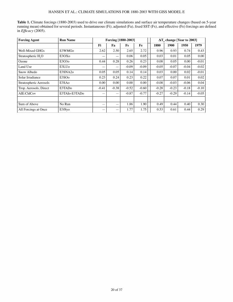
20 of 37


Table 1. Climate forcings (�880-2003) used to drive our climate simulations and surface air temperature changes (based on 5-year runningmean)obtainedforseveralperiods.Instantaneous(Fi),adjusted(Fa),fixedSST(Fs),andeffective(Fe)forcingsaredefinedin Efficacy (2005).

Forcing Agent Run Name Forcing [1880-2003] ΔTS change [Year to 2003]Fi Fa Fs Fe 1880 1900 1950 1979

Well-Mixed GHGs E3WMGo 2.62 2.50 2.65 2.72 0.96 0.93 0.74 0.43Stratospheric H2O E3OXo — — 0.06 0.05 0.03 0.0� 0.05 0.00Ozone E3O3o 0.44 0.28 0.26 0.23 0.08 0.05 0.00 -0.0�Land Use E3LUo — — -0.09 -0.09 -0.05 -0.07 -0.04 -0.02Snow Albedo E3SNA2o 0.05 0.05 0.�4 0.�4 0.03 0.00 0.02 -0.0�Solar Irradiance E3SOo 0.23 0.24 0.23 0.22 0.07 0.07 0.0� 0.02Stratospheric Aerosols E3SAo 0.00 0.00 0.00 0.00 -0.08 -0.03 -0.06 0.04Trop. Aerosols, Direct E3TADo -0.4� -0.38 -0.52 -0.60 -0.28 -0.23 -0.�8 -0.�0AIE:CldCov E3TAIo-E3TADo — — -0.87 -0.77 -0.27 -0.29 -0.�4 -0.05

Sum of Above No Run — — �.86 �.90 0.49 0.44 0.40 0.30All Forcings at Once E3f8yo — — �.77 �.75 0.53 0.6� 0.44 0.29

2� of 37


Table 2. Observed and simulated temperature change based on linear trend for indicated atmospheric levels and periods, with stan-dard deviations from 5-member ensembles.

(a) Temperature Trend (°C/decade)

Observations Model

Level Period Mears Christy Standard Forcings AltAer1 AltAer2 AltSol

Ocean A Ocean C Ocean C Ocean C Ocean C

MSU LS �979-2003 -0.32 -0.45 -0.30 ± 0.0� -0.3� ± 0.0� -0.30�±0.009 -0.305±0.0�0 -0.303±0.007

MSU T/S �987-2003 0.03 NA -0.006 ± 0.02 0.�0 ± 0.04 0.�02±0.036 0.�03±0.0�6 0.��3±0.025

MSU MT �979-2003 0.�3 0.05 0.�5 ± 0.0� 0.�4 ± 0.0� 0.�54±0.0�8 0.�48±0.02� 0.�5�±0.0�5

MSU LT �979-2003 0.�9 0.�2 0.20 ± 0.0� 0.�8 ± 0.0� 0.�97±0.02� 0.200±0.025 0.�97±0.0�7

GISS Jones

Surface �979-2003 0.�6 0.�8/0.�8 0.�48±0.0�4 0.�36±0.0�� 0.�47±0.0�7 0.�60±0.028 0.�53±0.0�7

(b) Temperature Change (°C)

GISS Jones

Surface �880-2003 0.60 0.73/0.73 0.697±0.005 0.528±0.044 0.749±0.035 0.7�2±0.038 0.639±0.0�9

Surface �900-2003 0.57 0.69/0.69 0.7�9±0.007 0.460±0.036 0.64�±0.034 0.623±0.030 0.554±0.036

Surface �950-2003 0.52 0.52/0.56 0.507±0.026 0.402±0.038 0.526±0.036 0.540±0.075 0.492±0.044

Surface �979-2003 0.38 0.43/0.44 0.355±0.034 0.325±0.027 0.354±0.04� 0.383±0.067 0.366±0.040

Mears and Christy’s observations are for �979 (or �987) through August 2005. Jones data are HadCRUT2/HadCRUT2v. HadCRUT2 is combined land and marine (SSTfromtheHadleyCentreoftheUKMeteorologicalOffice;seeRayneret al. [2003] for details) temperature anomalies on a 5°×5° grid-box basis. HadCRUT2v is a variance adjusted version of HadCRUT2.

Table 3.Globalsurfacetemperaturechanges(from5-yearrunningmean)obtainedwithalternativeoceanrepresentations,specifi-callyOceanA(observedoceansurfaceconditions)andOceanB(Q-fluxocean).

Forcing Agent Run Name Forcing [1880-2003] ΔTS change [Year to 2003]Fi Fa Fs Fe 1880 1900 1950 1979

Observed Ocean Model SST and Sea Ice E2OCN 0.00 0.00 0.00 0.00 0.57 0.53 0.42 0.28SST, Ice & All Forcings E3OCNf8 — — �.77 �.75 0.67 0.66 0.5� 0.3�SST, All Forcings E3SSTf8 — — �.77 �.75 0.62 0.56 0.45 0.30

Q-Flux ModelAll Forcings E3f8qd — — �.77 �.75 0.56 0.66 0.43 0.33

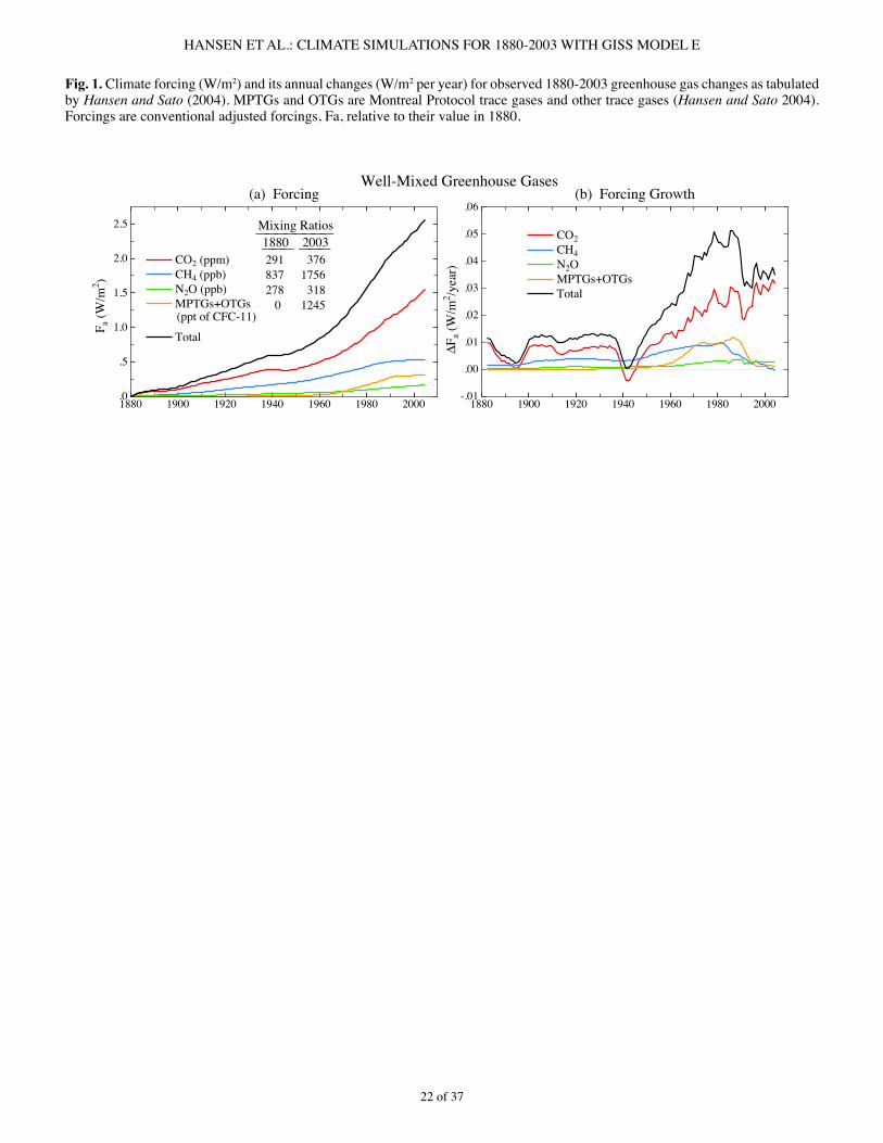
22 of 37


Fig. 1. Climate forcing (W/m2) and its annual changes (W/m2 per year) for observed �880-2003 greenhouse gas changes as tabulated by Hansen and Sato (2004). MPTGs and OTGs are Montreal Protocol trace gases and other trace gases (Hansen and Sato 2004). Forcings are conventional adjusted forcings, Fa, relative to their value in �880.

1880 1900 1920 1940 1960 1980 2000 .0

.5

1.0

1.5

2.0

2.5

CO2 (ppm)CH4 (ppb)N2O (ppb)MPTGs+OTGs

Total

(a) Forcing

F a (W

/m2 )

Well-Mixed Greenhouse Gases

Mixing Ratios1880 2003291 376837 1756278 318

0 1245(ppt of CFC-11)

1880 1900 1920 1940 1960 1980 2000-.01

.00

.01

.02

.03

.04

.05

.06

CO2CH4N2OMPTGs+OTGsTotal

(b) Forcing Growth

F a (W

/m2 /y

ear)

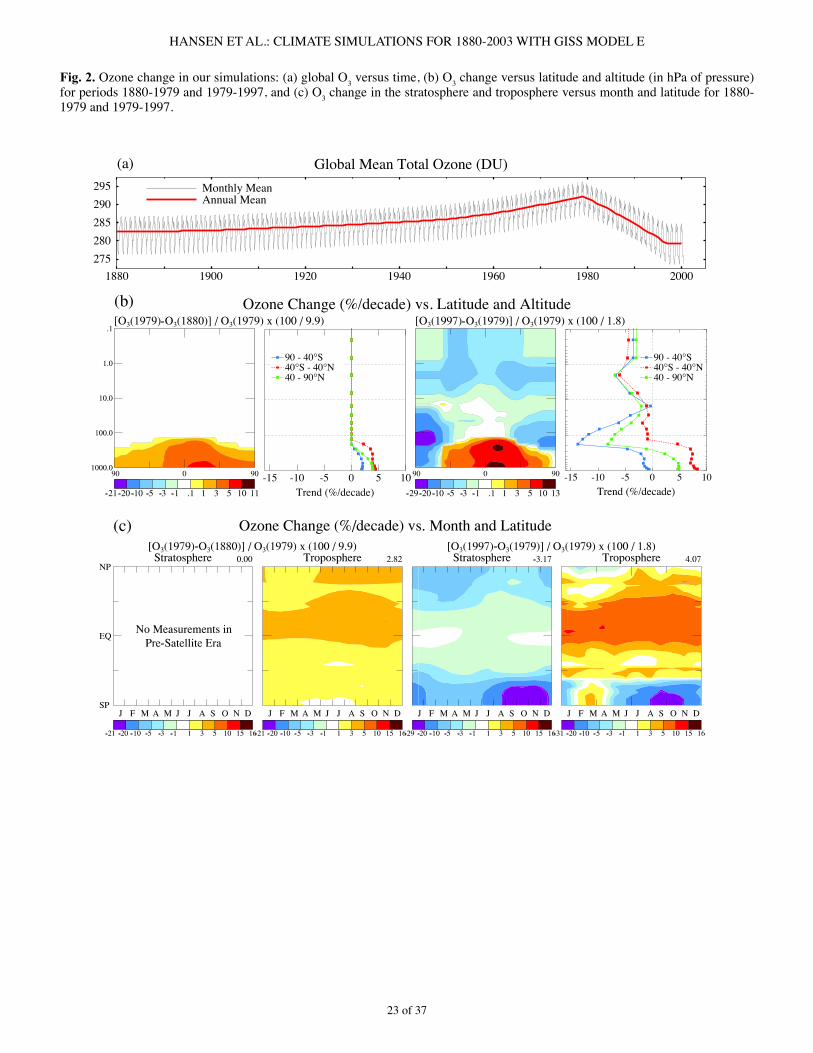
23 of 37


Fig. 2. Ozone change in our simulations: (a) global O3 versus time, (b) O3 change versus latitude and altitude (in hPa of pressure) for periods �880-�979 and �979-�997, and (c) O3 change in the stratosphere and troposphere versus month and latitude for �880-�979 and �979-�997.

1880 1900 1920 1940 1960 1980 2000 275 280 285 290 295 Monthly Mean

Annual Mean

Global Mean Total Ozone (DU)(a)

-15 -10 -5 0 5 10

90 - 40 S40 S - 40 N40 - 90 N

Ozone Change (%/decade) vs. Latitude and Altitude

Trend (%/decade)-15 -10 -5 0 5 10

90 - 40 S40 S - 40 N40 - 90 N

Trend (%/decade)

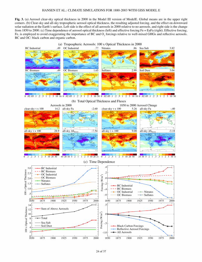
24 of 37


Fig. 3. (a) Aerosol clear-sky optical thickness in 2000 in the Model III version of ModelE. Global means are in the upper right corners. (b) Clear-sky and all-sky tropospheric aerosol optical thickness, the resulting adjusted forcing, and the effect on downward solar radiation at the Earth’s surface. Left side is the effect of all aerosols in 2000 relative to no aerosols, and right side is the change from �850 to 2000. (c) Time dependence of aerosol optical thickness (left) and effective forcing Fe = EaFa (right). Effective forcing, Fe, is employed to avoid exaggerating the importance of BC and O3forcingsrelativetowell-mixedGHGsandreflectiveaerosols.BC and OC: black carbon and organic carbon.

1850 1875 1900 1925 1950 1975 2000 .0

.5

1.0

1.5

2.0

2.5

3.0 BC IndustrialBC BiomassOC IndustrialOC BiomassNitratesSulfates

(c) Time Dependence

100

x O

ptic

al T

hick

ness

1850 1875 1900 1925 1950 1975 2000

-.6

-.4

-.2

.0

.2

.4

BC IndustrialBC BiomassOC IndustrialOC Biomass

NitratesSulfates

Forc

ing

(W/m

2 )

1850 1875 1900 1925 1950 1975 2000 0

2

4

6

8

10

12

14Sum of Above Aerosols

Sea SaltSoil Dust

Total

100

x O

ptic

al T

hick

ness

1850 1875 1900 1925 1950 1975 2000

-1.0

-.5

.0

.5

Black Carbon ForcingsReflective Aerosol ForcingsAll Aerosols

Forc

ing

(W/m

2 )

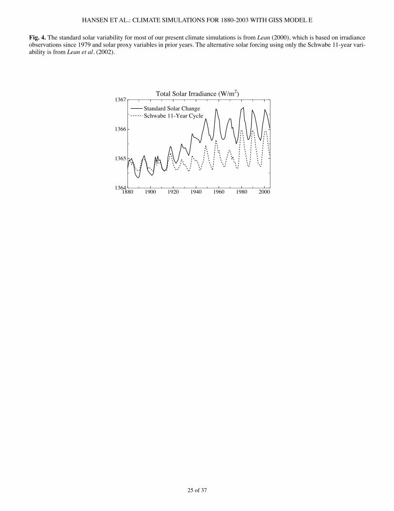
25 of 37


Fig. 4. The standard solar variability for most of our present climate simulations is from Lean (2000), which is based on irradiance observations since �979 and solar proxy variables in prior years. The alternative solar forcing using only the Schwabe ��-year vari-ability is from Lean et al. (2002).

1880 1900 1920 1940 1960 1980 20001364

1365

1366

1367Standard Solar ChangeSchwabe 11-Year Cycle

Total Solar Irradiance (W/m2)

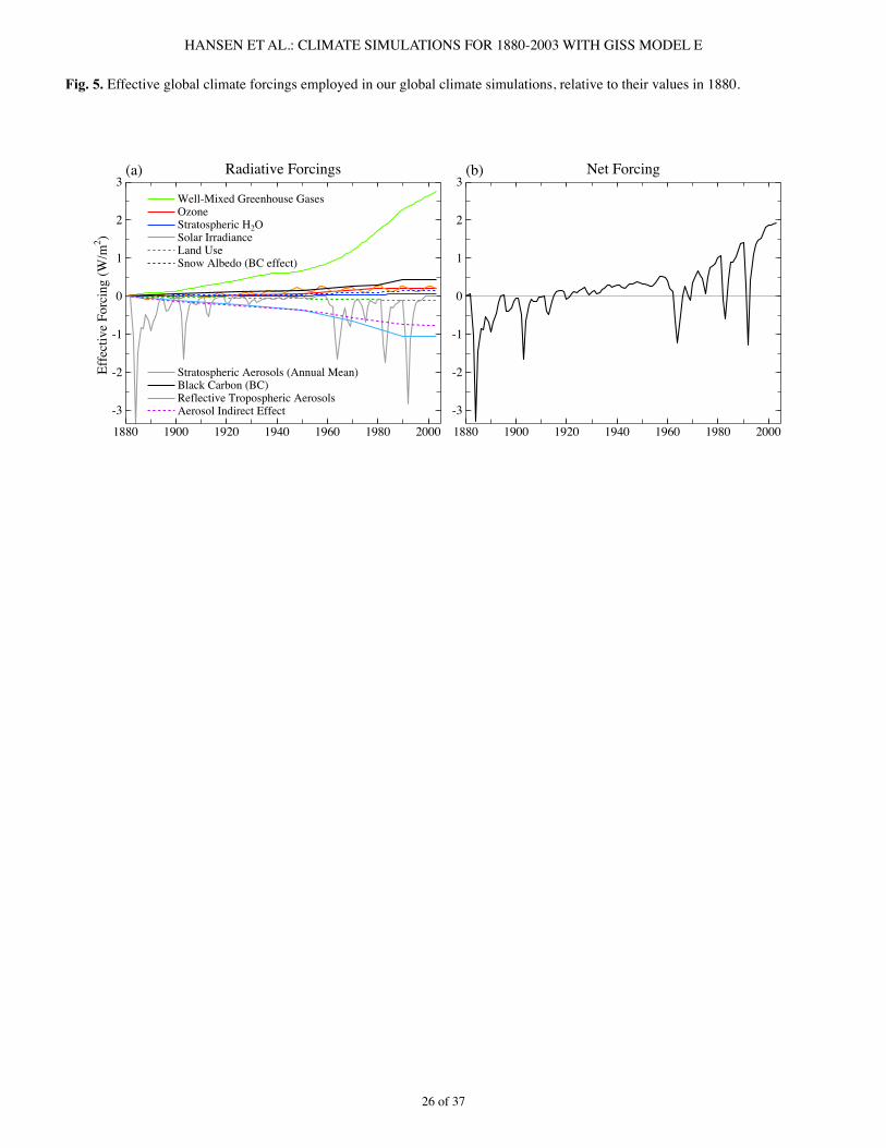
26 of 37


Fig. 5. Effective global climate forcings employed in our global climate simulations, relative to their values in �880.

1880 1900 1920 1940 1960 1980 2000

-3

-2

-1

0

1

2

3Well-Mixed Greenhouse GasesOzoneStratospheric H2OSolar IrradianceLand UseSnow Albedo (BC effect)

Stratospheric Aerosols (Annual Mean)Black Carbon (BC)Reflective Tropospheric AerosolsAerosol Indirect Effect

Radiative Forcings

Effe

ctiv

e Fo

rcin

g (W

/m2 )

(a)

1880 1900 1920 1940 1960 1980 2000

-3

-2

-1

0

1

2

3Net Forcing(b)

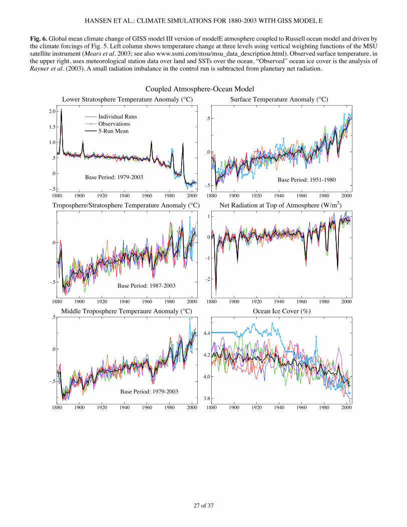
27 of 37


Fig. 6. Global mean climate change of GISS model III version of modelE atmosphere coupled to Russell ocean model and driven by the climate forcings of Fig. 5. Left column shows temperature change at three levels using vertical weighting functions of the MSU satellite instrument (Mears et al. 2003; see also www.ssmi.com/msu/msu_data_description.html). Observed surface temperature, in the upper right, uses meteorological station data over land and SSTs over the ocean. “Observed” ocean ice cover is the analysis of Rayner et al. (2003). A small radiation imbalance in the control run is subtracted from planetary net radiation.

1880 1900 1920 1940 1960 1980 2000 -.5

.0

.5

1.0

1.5

2.0Individual RunsObservations5-Run Mean

Lower Stratosphere Temperature Anomaly ( C)Coupled Atmosphere-Ocean Model

Base Period: 1979-2003

1880 1900 1920 1940 1960 1980 2000

-.5

.0

.5

Surface Temperature Anomaly ( C)


1880 1900 1920 1940 1960 1980 2000

-.5

.0

Troposphere/Stratosphere Temperature Anomaly ( C)


1880 1900 1920 1940 1960 1980 2000

-2

-1

0

1

Net Radiation at Top of Atmosphere (W/m2)

1880 1900 1920 1940 1960 1980 2000

-.5

.0

.5Middle Troposphere Temperaure Anomaly ( C)


1880 1900 1920 1940 1960 1980 2000

3.8

4.0

4.2

4.4

Ocean Ice Cover (%)

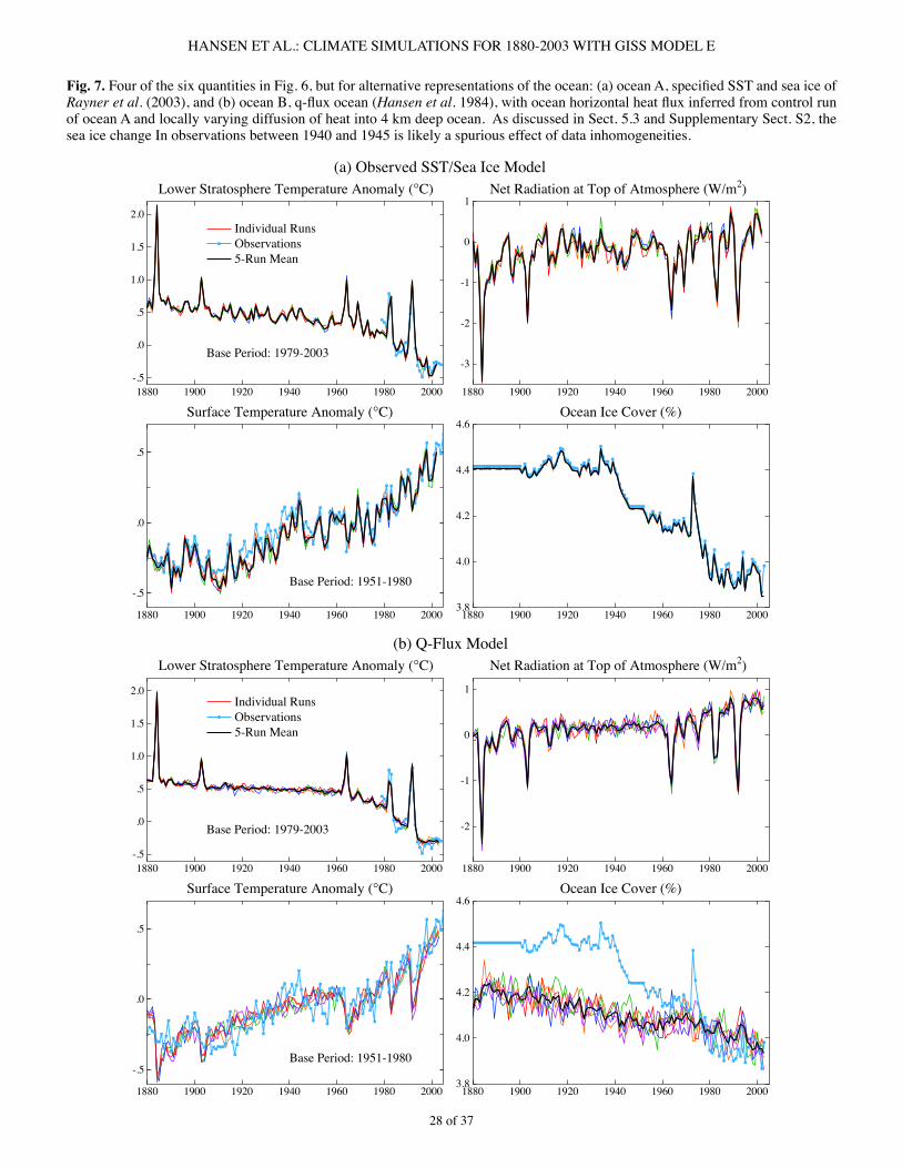
28 of 37


Fig. 7.FourofthesixquantitiesinFig.6,butforalternativerepresentationsoftheocean:(a)oceanA,specifiedSSTandseaiceofRayner et al.(2003),and(b)oceanB,q-fluxocean(Hansen et al.1984),withoceanhorizontalheatfluxinferredfromcontrolrunof ocean A and locally varying diffusion of heat into 4 km deep ocean. As discussed in Sect. 5.3 and Supplementary Sect. S2, the sea ice change In observations between �940 and �945 is likely a spurious effect of data inhomogeneities.

1880 1900 1920 1940 1960 1980 2000 -.5

.0

.5

1.0

1.5


Lower Stratosphere Temperature Anomaly ( C)(a) Observed SST/Sea Ice Model


1880 1900 1920 1940 1960 1980 2000

-3

-2

-1

0

1Net Radiation at Top of Atmosphere (W/m2)

1880 1900 1920 1940 1960 1980 2000

-.5

.0

.5



1880 1900 1920 1940 1960 1980 2000 3.8

4.0

4.2

4.4

4.6Ocean Ice Cover (%)

1880 1900 1920 1940 1960 1980 2000 -.5

.0

.5

1.0

1.5


Lower Stratosphere Temperature Anomaly ( C)(b) Q-Flux Model


1880 1900 1920 1940 1960 1980 2000

-2

-1

0

1

Net Radiation at Top of Atmosphere (W/m2)

1880 1900 1920 1940 1960 1980 2000

-.5

.0

.5



1880 1900 1920 1940 1960 1980 2000 3.8

4.0

4.2

4.4

4.6Ocean Ice Cover (%)

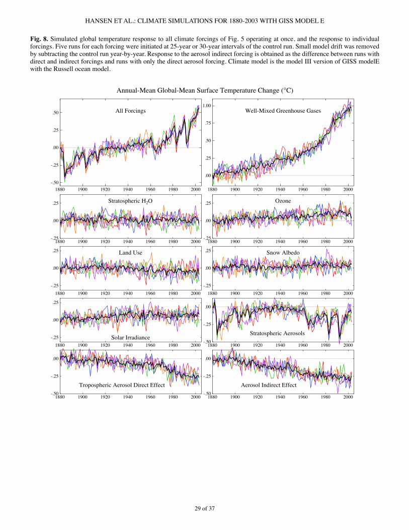
29 of 37


Fig. 8. Simulated global temperature response to all climate forcings of Fig. 5 operating at once, and the response to individual forcings. Five runs for each forcing were initiated at 25-year or 30-year intervals of the control run. Small model drift was removed by subtracting the control run year-by-year. Response to the aerosol indirect forcing is obtained as the difference between runs with direct and indirect forcings and runs with only the direct aerosol forcing. Climate model is the model III version of GISS modelE with the Russell ocean model.

1880 1900 1920 1940 1960 1980 2000-.50

-.25

.00

.25

.50 All Forcings

Annual-Mean Global-Mean Surface Temperature Change ( C)

1880 1900 1920 1940 1960 1980 2000

.00

.25

.50

.75

1.00Well-Mixed Greenhouse Gases

1880 1900 1920 1940 1960 1980 2000-.25

.00

.25 Stratospheric H2O

1880 1900 1920 1940 1960 1980 2000-.25

.00

.25 Ozone

1880 1900 1920 1940 1960 1980 2000-.25

.00

.25 Land Use

1880 1900 1920 1940 1960 1980 2000-.25

.00

.25 Snow Albedo

1880 1900 1920 1940 1960 1980 2000-.25

.00

.25

Solar Irradiance1880 1900 1920 1940 1960 1980 2000

-.50

-.25

.00

Stratospheric Aerosols

1880 1900 1920 1940 1960 1980 2000-.50

-.25

.00

Tropospheric Aerosol Direct Effect

1880 1900 1920 1940 1960 1980 2000-.50

-.25

.00

Aerosol Indirect Effect

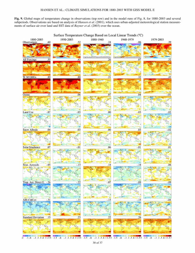
30 of 37


Fig. 9. Global maps of temperature change in observations (top row) and in the model runs of Fig. 8, for �880-2003 and several subperiods. Observations are based on analysis of Hansen et al. (200�), which uses urban-adjusted meteorological station measure-ments of surface air over land and SST data of Rayner et al. (2003) over the ocean.

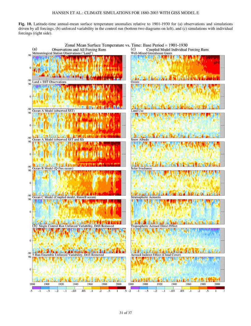
3� of 37


Fig. 10. Latitude-time annual-mean surface temperature anomalies relative to �90�-�930 for (a) observations and simulations driven by all forcings, (b) unforced variability in the control run (bottom two diagrams on left), and (c) simulations with individual forcings (right side).

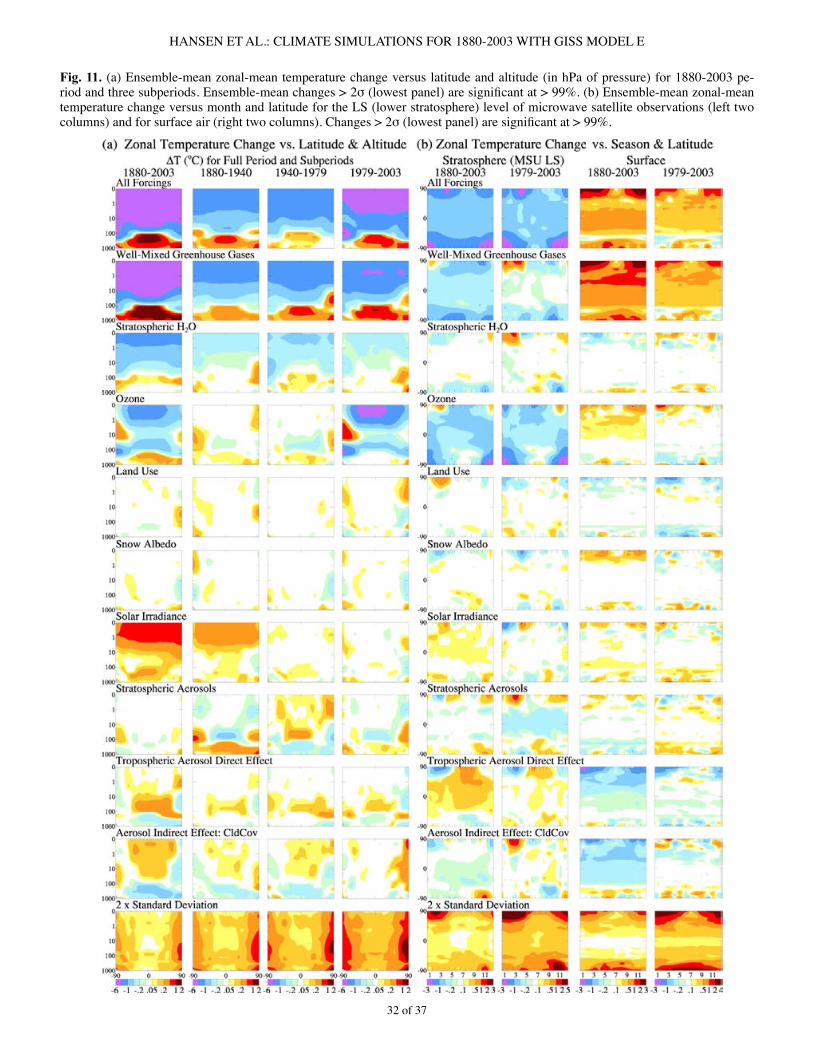
32 of 37


Fig. 11. (a) Ensemble-mean zonal-mean temperature change versus latitude and altitude (in hPa of pressure) for �880-2003 pe-riodandthreesubperiods.Ensemble-meanchanges>2σ(lowestpanel)aresignificantat>99%.(b)Ensemble-meanzonal-meantemperature change versus month and latitude for the LS (lower stratosphere) level of microwave satellite observations (left two columns)andforsurfaceair(righttwocolumns).Changes>2σ(lowestpanel)aresignificantat>99%.

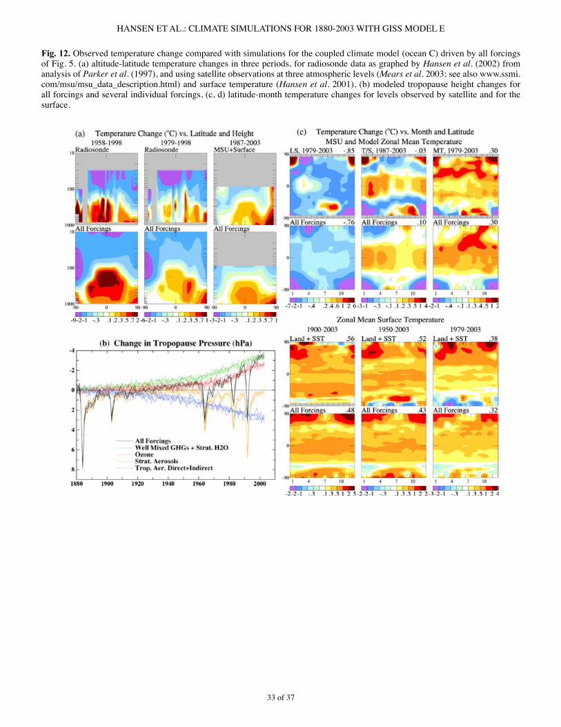
33 of 37


Fig. 12. Observed temperature change compared with simulations for the coupled climate model (ocean C) driven by all forcings of Fig. 5. (a) altitude-latitude temperature changes in three periods, for radiosonde data as graphed by Hansen et al. (2002) from analysis of Parker et al. (�997), and using satellite observations at three atmospheric levels (Mears et al. 2003; see also www.ssmi.com/msu/msu_data_description.html) and surface temperature (Hansen et al. 200�), (b) modeled tropopause height changes for all forcings and several individual forcings, (c, d) latitude-month temperature changes for levels observed by satellite and for the surface.

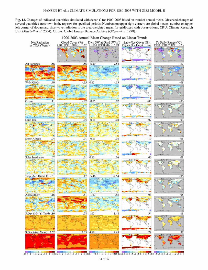
34 of 37


Fig. 13. Changes of indicated quantities simulated with ocean C for �900-2003 based on trend of annual mean. Observed changes of severalquantitiesareshowninthetoprowforspecifiedperiods.Numbersonupperrightcornersareglobalmeans;numberonupperleft corner of downward shortwave radiation is the area-weighted mean for gridboxes with observations. CRU: Climate Research Unit (Mitchell et al. 2004); GEBA: Global Energy Balance Archive (Gilgen et al. �998).

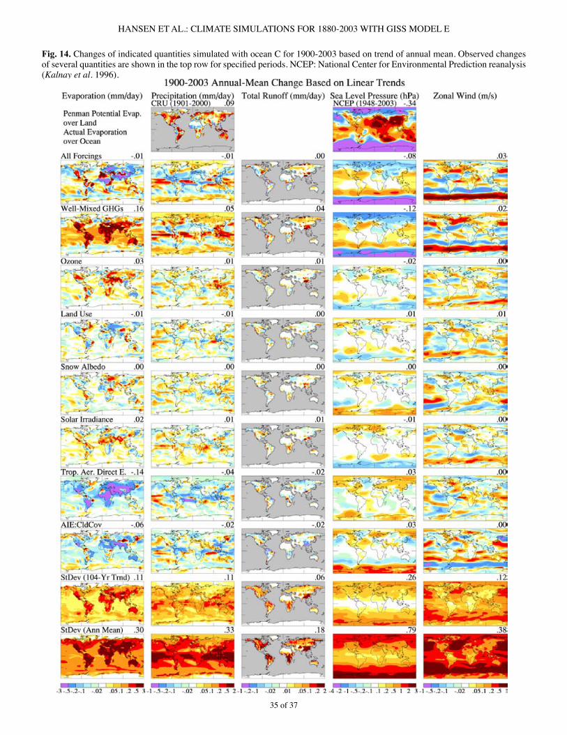
35 of 37


Fig. 14. Changes of indicated quantities simulated with ocean C for �900-2003 based on trend of annual mean. Observed changes ofseveralquantitiesareshowninthetoprowforspecifiedperiods.NCEP:NationalCenterforEnvironmentalPredictionreanalysis(Kalnay et al. �996).

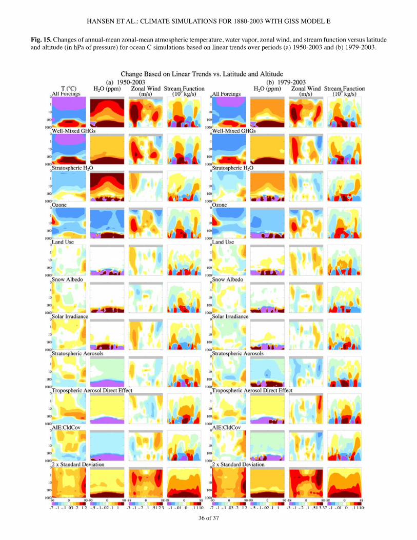
36 of 37


Fig. 15. Changes of annual-mean zonal-mean atmospheric temperature, water vapor, zonal wind, and stream function versus latitude and altitude (in hPa of pressure) for ocean C simulations based on linear trends over periods (a) �950-2003 and (b) �979-2003.

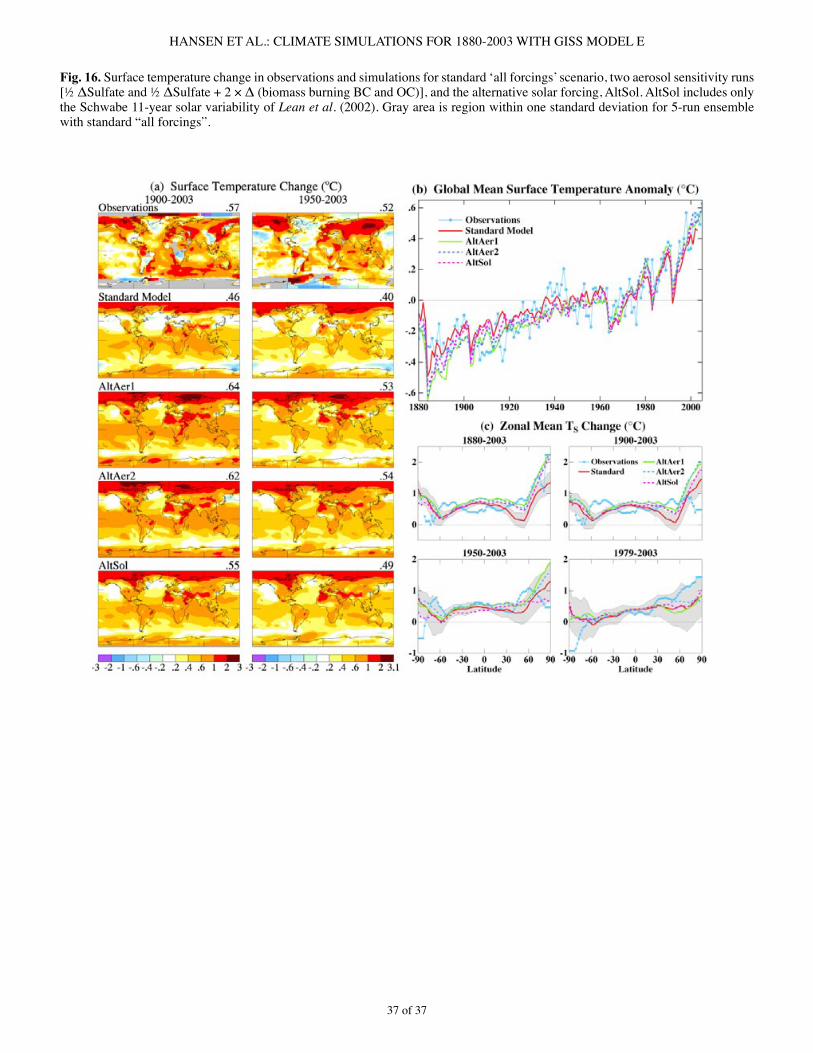
37 of 37


Fig. 16. Surface temperature change in observations and simulations for standard ‘all forcings’ scenario, two aerosol sensitivity runs [½ΔSulfateand½ΔSulfate+2×Δ(biomassburningBCandOC)],andthealternativesolarforcing,AltSol.AltSolincludesonlythe Schwabe ��-year solar variability of Lean et al. (2002). Gray area is region within one standard deviation for 5-run ensemble with standard “all forcings”.

S-� of S-7


Electronic Supplementary Material

for

Climate simulations for 1880-2003 with GISS modelE

by J. Hansen et al.

S1. Alternative Data Samplings and the Krakatau Problem Comparisons of simulated climate and observations com-monlyinvolvechoicesthatinflluencehowwellthemodelanddata appear to agree. Choices of surface temperature data de-serve scrutiny, because surface temperature provides the usual measure of long-term ‘global warming’ as well as a test of pos-sible global cooling after large volcanic eruptions. We illustrate here alternative comparisons of model and observations, with model results being those of the coupled model (ocean C, the Russell et al. [�995] model) driven by all climate forcings of Fig. 5. This model run is discussed in later sections.S1.1. Century time-scale Temperature measurements at meteorological stations pro-vide a reasonably consistent data set for continental and island locations (Jones et al. �986; Hansen and Lebedeff �987), albeit one in which the station records are spatially inhomogeneous, often broken temporally, and subject to non-climatic effects. The meteorological station records that we employ have been adjusted for urban effects using neighboring rural stations (Han-sen et al. 200�). Such adjustments are imperfect, but the impact on global mean �00-year temperature change of uncertainties in urban adjustments is not larger than about 0.�°C (IPCC 200�). For the short interval after a volcano considered here, urban ad-justments are negligible. The GISS analysis of station data (Hansen et al. �98�; Han-sen and Lebedeff �987) combines stations with overlapping peri-ods of record so as to preserve information on temporal variabil-ity while allowing individual stations to affect estimated temper-ature change at distances up to �200 km. It has been shown, by sampling a global model with realistic temperature variability at the station locations, that after about �880 the station network is capable of yielding a good estimate of global temperature change despite poor coverage in the Southern Hemisphere (Hansen and Lebedeff �987). However, island and coastal stations fail to sam-ple part of the ocean, and both observations and models indicate that the long-term temperature response tends to be less over the ocean than over continental areas. Thus we expect the long-term “global” temperature change estimated from the meteorological station network alone to slightly overestimate true global mean temperature change. Improved global coverage is obtained by combining me-teorological station data with sea surface temperature (SST) measurements of ocean areas (Jones et al. �999; Hansen et al. 200�). However, ocean data have their own problems, including changes of measurement methods and infrequent sampling of large regions (Parker et al. �994). Sampling is especially poor in the1800s,andspatial-temporaldata-fillproceduresrisksmooth-ing real variations. In addition, the ocean area with the largest response to climate forcings in climate models, regions of sea ice, are practically unobserved. Fig. S�a shows an estimate of global temperature using only meteorological station measurements (Hansen et al. 200�). The observed �880-2003 temperature change, based on the lin-

ear trend, is 0.69°C in this case. The model 5-run “all forcings” ensemble mean yields 0.56°C, with the model result being a true global mean. Fig. S�b uses the same land temperatures as in Fig. S�a, but it adds SST data for the oceans, using ship data of Rayner et al. (2003) for �880-�98� and subsequently satellite data (Reynolds and Smith �994; Smith and Reynolds 2004). Inclusion of ocean data reduces the observed global temperature change to 0.59°C. It also practically eliminates evidence for cooling after the �883 Krakatau eruption. Fig. S�c is a third alternative, comparing observed tempera-ture from meteorological stations with the model sampled at the places and times of the observations. This sampled model data is run through the same temperature analysis program as ob-servations to produce the global mean. This third procedure is optimum in the sense of having the most consistent treatment of model and data, as well as preserving a best estimate for high fre-quency temperature change in the period of sparse observations in the �800s. The model sampled at observing stations yields a global warming of 0.59°C based on the linear trend, which is less than the observed 0.69°C. This discrepancy occurs because the model warms less over land areas than observed, a result that we identify with excessive anthropogenic tropospheric aerosols over Eurasia in our standard “all forcings”, as discussed in Sect. 5. This third procedure provides a clean comparison of model and observations, but the integration over the globe is not a true global mean. In addition, it is unlikely that most modelers will sample their model results at the times and places of meteoro-logical station measurements and run the results through the GISStemperatureanalysisprogram,thusmakingitdifficulttocompare GISS model results with other models. Fig. S�d is a fourth alternative, comparing model results for the true global mean with observations that use only meteo-rological stations for �880-�900 but add ocean data for �900-2003, when ship data had better coverage. This alternative pre-serves temperature variations in the �800s without exaggerating long-term global temperature change. The observed �880-2003 temperature change in this case, 0.6�°C, is slightly larger than in Fig. S�b, as expected due to the cooling in the �880s. The disad-vantage of this fourth alternative is the arbitrariness inherent in concatenating two data sets. We present all four alternatives to help readers make their own assessment. For simplicity we use the procedure of Fig. S�b in following sections, i.e., we use the true global mean for the model and the land + ocean data for observations. However, it should be born in mind that these observations probably miss some actual cooling after Krakatau. We examine the Krakatau period in more detail, because it has an effect on how well the model and observations appear to agreeoverthe120-yeartemperaturerecord.Wefinditusefultocompare the �883 Krakatau and �99� Pinatubo eruptions, the two largest volcanic aerosol climate forcings in the period of in-strumental climate data (Sato et al. �993). These volcanoes have the best chance of producing signals above the climate noise lev-el and the Pinatubo period has extensive climate observations.S1.2. Temperature change after Krakatau and Pinatubo Estimated aerosol optical depths after Krakatau and Pintubo are shown in Fig. S2a. The shape of the Krakatau curve is as-sumed to be similar to that after Pinatubo, as they were both low latitude injections to high altitudes at similar times of year. Measurements of decreased solar irradiance integrated over

S-2 of S-7


three years after Krakatau were used to set the aerosol optical depth (Sato et al. �993). Effective forcings are shown in Fig. S2b. Resulting temperature anomalies, relative to the three-year mean preceding the eruption, are shown in Fig. S2c. The simu-lated cooling after Krakatau exceeds that after Pinatubo by more than the assumed �0% difference in their forcings. This must be at least in part because of planetary radiation imbalance of about +0.5 W/m2 that existed just prior to the Pinatubo eruption (Hansen et al. �993) but not at the time of the Krakatau erup-tion. Further, as mentioned in Sect. 3.2.�, the response to the Krakatau aerosols would have been reduced about �0 percent if the control run ocean temperatures had included the effect of prior volcanic eruptions via a mean stratospheric aerosol optical depth. Fig. S2c shows that the global mean temperature based on meteorological station data after Krakatau is consistent with the climatesimulations.Theseasonalmean1σerrorbarforglobaltemperature estimated from the meteorological station network in the �880s is 0.�5°C (Hansen and Lebedeff �987). Thus the cooling observed by the station network after Krakatau for a giv-en season could be a sampling error, but not the nearly continu-ous cool period for several years after the eruption. Furthermore, comparison of the global temperature curve estimated from me-teorological stations in the Pinatubo era (right side of Fig. S2c) with the global temperature curve that has complete ocean cov-erage from satellite data shows that the station network tracks the complete global data within the expected error for the station network(1σsamplingerrorbeing0.09°Cforthestationdistri-bution in the �990s). We conclude that there was global cooling after Krakatau. Fig. S2d shows the observed and simulated surface temper-ature anomalies in the northern winter (DJF) following the erup-tions and the northern summer (JJA) about one year after the eruptions. As expected, the model and observations show strong cooling in the summer after the eruption, especially over the con-tinents. Also, the model and observations show global cooling in DJF, with evidence for regional Eurasian “winter warming”, an expected dynamical response (Groisman �992; Perlwitz and Graf �995; Robock 2000; Shindell et al. 200�), which has previ-ously been reported to occur in current GISS models (Shindell et al. 2004). The model, using the coarse-resolution Russell et al. (�995) ocean, is not able to produce El Ninos, which have ac-companied several large volcanoes in the past century (Handler �984; Robock 2000; Mann et al. 2005) and may be responsible for warming in the region of Alaska. Temperature anomalies are muted in the 5-run model mean in Fig. S2d, but the magnitude of anomalies is more realistic in the individual runs, which are available on the GISS web-site.S2. Mean Stratospheric Aerosols in Control Run Our control run had no stratospheric aerosols. Aerosols from the �883 Krakatau eruption caused ocean heat content in the experiment runs to fall below that in the control run, as ex-pected. However, despite steadily increasing greenhouse gases, the ocean heat content did not recover to that of the control run untilabout2000.Inreality,oceantemperatureisalsoinfluencedby volcanoes that erupted prior to �880. Ideally, ocean initial conditions in �880 would be obtained from a spin-up run that had time-dependent forcings, including volcanoes, for several centuries prior to �880. That is not usually practical, if for no other reason than the absence of information on earlier volcanic eruptions. However, it is easy to include a mean stratospheric

aerosol amount in the control run. Current control runs with our model include a mean strato-sphericaerosolopticalthicknessτ=0.0125at0.55μmwave-length, which is the �850-2000 mean value of the Sato et al. (�993) aerosol climatology. The equilibrium global (surface) coolingforτ=0.0125(10%of themaximumτforPinatubo)is ~0.2°C, and the effect on deeper ocean temperatures is suf-ficienttoaltertherateofoceanheatstorageintransientclimatesimulations. Using a control run in which the ocean temperature had equilibrated with an atmosphere including this mean aero-sol amount, we carried out an ensemble of runs for �850-2003. The concentration of volcanoes near the end of the �9th century caused the ocean heat content anomaly to be negative for several decades, but it recovered to the control run value by the mid 20th century and it subsequently increased at a rate comparable to that reported by Levitus et al. (2000).S3. Control Run Disequilibrium and Drift. Our coupled atmosphere-ocean (ocean C) simulations, to meet the deadline for submission to IPCC, were initiated be-fore the control run (which provides initial conditions for the experiments) had reached equilibrium, i.e., while there was still an imbalance between the amounts of energy absorbed and emit-ted by the planet. As a result, the model response to any forcing included a small drift. We minimize drift effects by subtracting, year-by-year, the same quantities from the same period of the control run. This procedure yields diagnostics with ‘double noise’, i.e., it contains unforced variability of both the control and experiment runs, while the real world has only a single source of unforced vari-ability. Double noise can be minimized by initiating additional control runs at the same points at which experiments are initi-ated. An alternative way to remove drift is to calculate and sub-tract from the experiment result the mean drift in the control over the period of the experiment. For example, for a �24-year �880-2003 experiment initiated at year X of the control run, we could calculate the linear trends of control run diagnostics over the period X to X + �23 and subtract the control run diagnostics based on their linear trends from the corresponding quantities in the experiment run. This alternative procedure avoids year-to-year double noise, but it does not eliminate drift effects entirely because variability occurs on all time scales. Noise effects were exacerbated by the fact that most of our experiments, with individual forcings and with multiple forc-ings, were initiated at the same points of the control run. The control run has unforced variability not only interannually, but on �24-year and all other time scales. Thus when we add up responses to individual forcings, with drift subtracted, we are in-cludingthesameunforced124yearfluctuationforeachforcing.Therefore we cannot expect the sum of the responses to indi-vidual forcings to equal the response to the sum of the forcings, even if there is no non-linearity in the climate response. An improved procedure would be to initiate experiments for different forcings at different points on the control run, in addition to spacing ensemble members. It would perhaps be still better to carry out a long control run that reaches equilibrium before experiments are initiated, so there would be no need to subtract a control run. However, the merits of waiting until the control run equilibrates before initiating experiments may be reduced if the equilibrium climate drifts too far from the real world.

S-3 of S-7


S4.SurfaceTemperatureDefinition. Surface air temperature (Ts) in modelE is calculated at �0 m height. The land-ocean temperature index (Tx) (Hansen et al. 200�) is from observations at 2 m height at meteorological stations and SST data of Rayner et al. (2003) and Reynolds and Smith (�994) over the ocean. Temperature changes of model and observations are compared, which minimizes, but does not eliminate, the effect of these height differences. Fig. S3 shows the modeled �880-2003 temperature change for (�) ocean A driven by no forcings except SST and sea ice change, (2) the same as (�) but including “all forcings” (GHGs, aerosols, etc.), (3) the same as (2), but for the coupled atmo-sphere-ocean climate model. For each of these three models we show the global surface air temperature (Ts), the temperature index (Tx), which uses the ocean temperature instead of Ts for ocean areas, and their difference. In the case of ocean A with no forcings, Ts and Tx are prac-tically the same on global average, even though there are regions where they differ by a few tenths of a degree. In the case of ocean A with radiative forcings, the forcings are able to change atmospheric temperature slightly even though SST is fixed.Global mean Ts increases 0.03ºC more than Tx increases over the period �880-2003. In the case of ocean C the ocean tempera-ture is able to respond to the change of near surface temperature gradient, and Ts increases 0.05ºC more than Tx increases over the �880-2003 period. These comparisons indicate that our use of global Ts at �0 mheightoverstatesglobalmean∆Tbyseveralhundredthsofadegree, if our aim is comparison with a temperature index that usesSSTs.Wecouldemploy∆Txfromthemodelbasedonthefirstlayeroceantemperature,butthatwouldbeinconsistentwiththe procedure used in previous studies with the GISS model and othermodels, and thuswe used∆Ts in this paper.This issuemay be noticeable only in the GISS model, which calculates Ts in an iterative fashion (Hansen et al. �983; modelE 2006). In the future the issue might be practically eliminated by calculating Ts at 2 m height, rather than �0 m. These small changes in∆T do not alter the geographicalpattern of the discrepancy between model and observations. The main implication is that the �24-year warming in our model with “all forcings” is ~0.�0ºC less than observed, rather than 0.05ºC less. Thus the need for less tropospheric aerosol amount becomes clearer in the global mean temperature, as well as from unrealistic cooling over Europe. As future models are better able to simulate observed cli-mate change, it will be worth removing any such discrepancy in comparison with observed surface temperature. We are un-certain whether this comparison issue exists for other climate models.S5. Ozone Scenario. ThefirstsetofrunsthatweprovidedtoIPCCinadvertentlyused the Randel and Wu (�999) decadal rate of stratospheric O3 depletion as the �8-year change, thus understating stratospheric O3 depletion by the factor �0/�8. Corrected runs were submit-ted several months later, and both sets of runs remain available at www-pcmdi.llnl.gov/ipcc/about_ipcc.php. The correction re-duced the �880-2003 global forcing Fa by 0.03 W/m2. The main impact of the correction was on stratospheric cooling in the Ant-arctic region during the time of O3 depletion, with the corrected results providing better agreement with observations. The pres-ent paper and Efficacy (2005) use the corrected O3 change.

A second issue with the O3 scenario concerns O3 forcing due to tropospheric pollution. The O3 scenario was derived from an off-line simulation of a tropospheric chemistry model (Shindell et al. 2003), which yielded an �880-2000 O3 change from the surface to the �50 hPa level at all latitudes. Global forcings for this O3 change were Fi = 0.44, Fa = 0.38 W/m2. However, tropo-spheric O3 forcing implemented in our transient simulations was less, as high-latitude O3 increases above the model’s tropopause (Fig. 3 of Efficacy [2005]) were excluded, reducing O3 forcing by 0.05 W/m2. As the pollution effect on O3 at low latitudes was only allowed to reach the �50 hPa level, we suspect that our total O3 forcing (Fa = 0.28, Fs = 0.26, Fe = 0.23 W/m2, including tropospheric pollution and stratospheric depletion, from Table �) underestimates actual O3 forcing. Future O3 scenarios should be generated by models with improved vertical resolution and higher model top, preferably integrating effects of tropospheric pollution and stratospheric change.S6. Snow Albedo. A computer programming error was present in the calcula-tion of snow albedo in several of our climate simulations. Some of these runs were repeated with the error corrected, as delineat-ed below. Our intention was for snow albedo change to be pro-portional to BC deposition as calculated by the aerosol transport model of Koch (200�). The error caused albedo change to be exaggerated in partially snow-covered land gridboxes and un-derstatedoverseaice,becausetotalalbedochangewasfixed. Our initial ‘all forcing’ run provided to IPCC contained both the ozone error (A.4) and snow albedo error (A.5). We also pro-vided to IPCC ‘all forcing’ runs with the ozone error corrected and later runs with both errors corrected. Because of space limi-tations, the DOE web site includes only the original ‘all forcing’ ensemble and the ensemble with the ozone forcing corrected. All three ensembles are available on the GISS web site. The ‘all forcing’ and snow albedo alone ensembles were rerun with the snow albedo error corrected. The corrected pro-gram was also used in ‘Arctic pollution’ runs (Fig. 5 in Danger-ous [2006]). However, the AltAer�, AltAer3, and AltSol runs contain the snow albedo error, but not the ozone error. These ensembles were not rerun with corrected snow albedo because of the small magnitude of the error and the fact that it would not alter conclusions from those runs. To allow precise comparison with AltAer�, AltAer2, and AltSol, the standard model results in Fig. �6 of this paper and Fig. 6 in Dangerous (2006) are the ‘all forcing’ results that include the snow albedo error. The simulations employed in the energy imbalance study of Hansen et al. (2005b) contained both errors. The errors in global forcing, +0.03 W/m2 and –0.02 W/m2, opposed each other, but regional and temporal effects would not cancel, e.g., strato-spheric cooling over Antarctica was underestimated. However, the magnitude of these errors is too small to affect conclusions of that paper. Efficacy (2005) simulations included the snow albedo error but not the ozone error. In Table 4 and Fig. �6 of Efficacy (2005) the snow albedo forcing was calculated with the incorrect pro-gram. Fa was actually 0.05 W/m2, not 0.08 W/m2, and the correct efficacyforthesnowalbedoeffectwasEa~2.7,notEa~1.7.

References to Supplementary MaterialGroisman PY (�992) Possible climate consequences of the Pinatubo

eruption: An empirical approach. Geophys Res Lett �9:�603—�606.Handler P (�984) Possible association of stratospheric aerosols and El

Nino type events. Geophys Res Lett ��:��2�—��24.

S-4 of S-7


Hansen J, Johnson D, Lacis A, Lebedeff S, Lee P, Rind D, Russell G (�98�) Climate impact of increasing atmospheric carbon dioxide. Sci-ence 2�3:957—966.

Hansen J, Russell G, Rind D, Stone P, Lacis A, Lebedeff S, Ruedy R, TravisL(1983)Efficientthree-dimensionalglobalmodelsforclimatestudies: Models I and II. Mon Weather Rev ��:609—662.

Hansen J, Lebedeff S (�987) Global trends of measured surface air tem-perature. J Geophys Res 92:�3345—�3372.

Hansen J, Lacis A, Ruedy R, Sato M, Wilson H (�993) How sensitive is the world’s climate? Natl Geogr Res Explor 9:�42—�58.

Hansen J, Ruedy R, Glascoe J, Sato M (�999) GISS analysis of surface temperature change. J Geophys Res �04:30997-3�022.

Hansen J, Ruedy R, Sato M, Imhoff M, Lawrence W, Easterling D, Peterson T, Karl T (200�) A closer look at United States and global surface temperature change. J Geophys Res �06:23947—23963.

HansenJetal(2005a)Efficacyofclimateforcings.JGeophysRes110:D�8�04. DOI �0.�029/2005JD005776.

HansenJetal(2005b)Earth’senergyimbalance:confirmationandim-plications. Science 308:�43�—�435.

Hansen J et al (2006b) Dangerous human-made interference with cli-mate: A GISS modelE study. Atmos Chem Phys Discuss 6:�2549—�26�0.

Intergovernmental Panel on Climate Change (IPCC) (200�) Climate Change2001:TheScientificBasis.HoughtonJT,DingY,GriggsDJ,Noguer M, van der Linden PJ, Dai X, Maskell K, Johnson CA (eds) Cambridge University Press, Cambridge, UK.

Jones PD, Wigley TML, Wright PB (�986) Global temperature varia-tions between �86� and �984. Nature 322:430—434.

Jones PD, New M, Parker DF, Martin S, Rigor LG (�999) Surface air temperature and its changes over the past �50 years. Rev Geophys 37:�73—�99.

Koch D (200�) Transport and direct radiative forcing of carbonaceous and sulfate aerosols in the GISS GCM. J Geophys Res �06:203��—20332.

Levitus S, Antonov J, Boyer TP, Stephens C (2000) Warming of the world ocean. Science 287:2225—2229.

Mann ME, Cane MA, Zebiak SE, Clement A (2005) Volcanic and so-lar forcingof the tropicalPacific over the past 1000years. JClim�8:447—456.

Parker DE, Jones PD, Folland CK, Bevan A (�994) Interdecadal chang-es of surface temperature since the late nineteenth century. J Geophys Res 99:�4373—�4399.

Perlwitz J, Graf HF (�995) The statistical connection between tropo-spheric and stratospheric circulation of the Northern Hemisphere in winter. J Clim 8:228�—2295.

Randel WJ, Wu F (�999) A stratospheric ozone trends data set for glob-al modeling studies. Geophys Res Lett 26:3089—3092.

Rayner NA, Parker DE, Horton EB, Folland CK, Alexander LV, Rowell DP, Kent EC, Kaplan A (2003) Global analyses of SST, sea ice and night marine air temperatures since the late nineteenth century. J Geo-phys Res �08(D�4):4407. DOI �0.�029/2002JD002670.

Reynolds RW, Smith TM (�994) Improved global sea surface tempera-ture analyses, J Clim 7:929—948.

Robock A (2000) Volcanic eruptions and climate. Rev Geophys 38:�9�—2�9.

Russell GL, Miller JR, Rind DH (�995) A coupled atmosphere-ocean model for transient climate change. Atmos Ocean 33:683—730.

Sato M, Hansen J, McCormick MP, Pollack JP (�993) Stratospheric aerosol optical depths, �850-�990. J Geophys Res 98:22987—22994.

Schmidt GA et al (2006) Present day atmospheric simulations using GISS ModelE: Comparison to in-situ, satellite and reanalysis data. J Clim �9:�53—�92.

Shindell D, Schmidt GA, Miller RL, Rind D (200�) Northern Hemi-sphere winter climate response to greenhouse gas, volcanic, ozone and solar forcing. J Geophys Res �06:7�93—72�0.

Shindell DT, Fulavegi G, Bell N (2003) Preindustrial-to-present-day radiative forcing by tropospheric ozone from improved simulations with the GISS chemistry-climate GCM. Atmos Chem Phys 3:�675—�702.

Shindell DT, Schmidt GA, Mann ME, Fulavegi G (2004) Dynamic win-ter climate response to large tropical volcanic eruptions since �600. J Geophys Res �09:D05�04. DOI �0.�029/2003JD004�5�.

Smith TM, Reynolds RW (2004) Improved extended reconstruction of SST (�854-�997). J Clim �7:2466—2477.

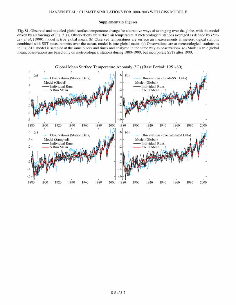
S-5 of S-7


Supplementary Figures

Fig. S1. Observed and modeled global surface temperature change for alternative ways of averaging over the globe, with the model drivenbyallforcingsofFig.5.(a)ObservationsaresurfaceairtemperatureatmeteorologicalstationsaveragedasdefinedbyHan-sen et al. (�999), model is true global mean. (b) Observed temperatures are surface air measurements at meteorological stations combined with SST measurements over the ocean, model is true global mean. (c) Observations are at meteorological stations as in Fig. S�a, model is sampled at the same places and times and analyzed in the same way as observations. (d) Model is true global mean, observations are based only on meteorological stations during �880-�900, but incorporate SSTs after �900.

1880 1900 1920 1940 1960 1980 2000

-.6

-.4

-.2

.0

.2

.4

.6

.8

Observations (Station Data)

Individual Runs5 Run Mean

Global Mean Surface Temperature Anomaly ( C) (Base Period: 1951-80)

Model (Global)

(a)

1880 1900 1920 1940 1960 1980 2000

-.6

-.4

-.2

.0

.2

.4

.6Observations (Land+SST Data)


Model (Global)

(b)

1880 1900 1920 1940 1960 1980 2000

-.6

-.4

-.2

.0

.2

.4

.6Observations (Station Data)


Model (Sampled)

(c)

1880 1900 1920 1940 1960 1980 2000

-.6

-.4

-.2

.0

.2

.4

.6Observations (Concatenated Data)


Model (Global)

(d)

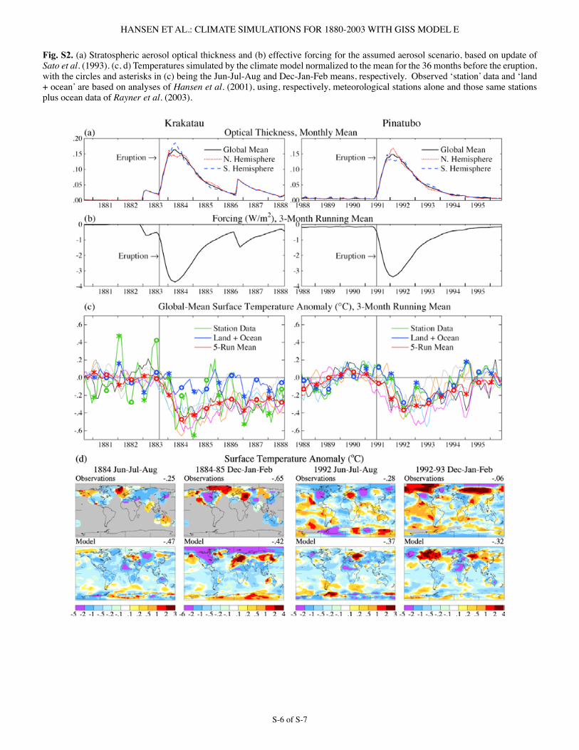
S-6 of S-7


Fig. S2. (a) Stratospheric aerosol optical thickness and (b) effective forcing for the assumed aerosol scenario, based on update of Sato et al. (�993). (c, d) Temperatures simulated by the climate model normalized to the mean for the 36 months before the eruption, with the circles and asterisks in (c) being the Jun-Jul-Aug and Dec-Jan-Feb means, respectively. Observed ‘station’ data and ‘land + ocean’ are based on analyses of Hansen et al. (200�), using, respectively, meteorological stations alone and those same stations plus ocean data of Rayner et al. (2003).

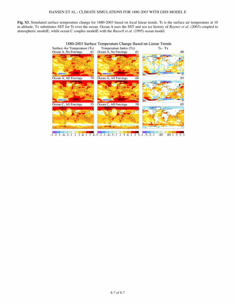
S-7 of S-7


Fig. S3. Simulated surface temperature change for �880-2003 based on local linear trends. Ts is the surface air temperature at �0 m altitude, Tx substitutes SST for Ts over the ocean. Ocean A uses the SST and sea ice history of Rayner et al. (2003) coupled to atmospheric modelE, while ocean C couples modelE with the Russell et al. (�995) ocean model.

Climate simulations for 1880���2003 with GISS modelE

Documents

Climate simulations for 1880��2003 with GISS modelE