Classical Physics and Quantum Loops

arX

iv:h

ep-t

h/04

0523

9v1

26

May

200

4

Classical Physics and Quantum Loops

Barry R. Holsteina,b and John F. Donoghuea

a Department of Physics-LGRTUniversity of Massachusetts

Amherst, MA 01003b Theory Group

Thomas Jefferson National Accelerator Laboratory12000 Jefferson Ave.

Newport News, VA 23606

February 1, 2008

Abstract

The standard picture of the loop expansion associates a factor of hwith each loop, suggesting that the tree diagrams are to be associatedwith classical physics, while loop effects are quantum mechanical innature. We discuss examples wherein classical effects arise from loopcontributions and display the relationship between the classical termsand the long range effects of massless particles.

1

1 Introduction

It is commonly stated that the loop expansion in quantum field theory isequivalent to an expansion in h. Although this is mentioned in several fieldtheory textbooks, we have not found a fully compelling proof of this state-ment. Indeed, no compelling proof is possible because the statement is nottrue in general. In this paper we describe several exceptions - cases whereclassical effects are found within one loop diagrams - and discuss what goeswrong with purported “proofs”.

Most physicists performing quantum mechanical calculations eschew keep-ing track of factors of h, and use units wherein h is set to unity—only whennumerical results are needed are these factors restored. However, use of thisprocedure can cloak the difference between classical and quantum mechani-cal effects, since the former are distinguished from the latter merely by theabsence of factors of h. This is also the practice in many field theory texts,but there is often a discussion in such works about a one to one connectionbetween the number of loops and the factors of h[1]. The argument used inorder to make this connection is a simple one, and is worth outlining here: Incalculating a typical Feynman diagram, the presence of a vertex arises fromthe expansion of

expi

h

∫

Lint(φin)d4x

and so carries with it a factor of h−1. On the other hand the field commuta-tion relations

[φ(~x), π(~y] = ihδ3(~x − ~y)

lead to a factor of h in each propagator

< 0|T (φ(x)φ(y))|0 >=∫

d4k

(2π)4

iheik(x−y)

k2 − m2

h2 − iǫ

The counting of factors of h then involves calculating the number of verticesand propagators in a given diagram. For a diagram with V vertices and Iinternal lines the number of independent momenta is L = I − V + 1 andcorresponds to the number of loops. Associating a factor of h−1 for the Vvertices and h+1 for the I propagators yields an overall factor

hI−V +1 = hL

1

which is the origin of the claim that the loop expansion coincides with anexpansion in h. We shall demonstrate in the next section, however, that thisassertion in not valid.

2 A counterexample

Let us give an example where one obtains classical results from a one-loopcalculation. This example is chosen because it is easy to identify the classicaland quantum effects. We describe the one-loop QED calculation of the matrixelement of the energy- momentum tensor between initial and final plane wavestates[2]. For simplicity, we shall discuss below the case wherein these statesare spinless, but the calculation was performed also for spin 1/2 systems andthe results are the same.

The basic structure of the matrix element is given by

< p2|Tµν(0)|p1 >=1√

4E2E1

[2PµPνF1(q2) + (qµqν − ηµνq

2)F2(q2)] (1)

where F1(q2), F2(q

2) are form factors, to be determined. In lowest order theenergy-momentum tensor form factors are

F1(q2) = 1, F2(q

2) = −1

2, (2)

but these simple results are modified by loops, and the form factors willreceive corrections of order e2 at one loop order. One can evaluate thesemodifications using the diagrams shown in Figure 1, and the results arefound to be[2]

F1(q2) = 1 +

e2

16π2

q2

m2

(

3

4

mπ2

√−q2

− 8

3+ 2 log

−q2

m2− 4

3log

λ

m

)

+ . . .

F2(q2) = −1

2+

e2

16π2

(

mπ2

2√−q2

− Ω − 26

9+

4

3log

−q2

m2

)

+ . . . (3)

where

Ω =2

ǫ− γ − log

m2

4πµ2(4)

The factors of h will be inserted in the discussion of the next section.

2

(a) (b) (c) (d)

(e)X

(f) (g)X(h)

Figure 1: Feynman diagrams for spin 0 radiative corrections to Tµν .

3

It is easiest to separate the classical and quantum effects by going tocoordinate space via a Fourier transform. The key terms are those that have

a nonanalytic structure such as√

−q2/m2 and q2 ln−q2. These both ariseonly from those diagrams where the energy momentum tensor couples tothe photon lines. In particular, the square root term comes uniquely fromFigure 1c. We will see that the square root turns into a well known classicalcorrection while the logarithm generates a quantum correction. Specificallywe take the transform

Tµν(~r) =∫ d3q

(2π)3ei~q·~rTµν(~q) (5)

Using∫

d3q

(2π)3ei~q·~r|~q| = − 1

π2r4

as well as∫

d3q

(2π)3ei~q·~r~q2 log ~q2 =

3

πr5

and including powers of h in the result, we find

T00(~r) = mδ3(~r) +e2

32π2r4− e2h

4π3mr5+ . . .

T0i(~r) = 0

Tij(~r) = − e2

16π2r4

(

rirj

r2− 1

2δij

)

− e2h

16π3mr5(3δij − 5

rirj

r2) + . . . (6)

We see then that Eq. 6 includes both corrections which are independent ofh as well as pieces which are linear in this quantity.

The interpretation of the classical terms is clear. Since the energy-momentum tensor for the electromagnetic field has the form[3]

TEMµν = −FµλFν

λ +1

4ηµνFλδF

λδ (7)

and, for a simple point charge, we have

E =e

4πr2r

4

we determine

TEM00 (~r) =

1

2E2 =

e2

32π2r4

TEM0i (~r) = 0 (8)

TEMij (~r) = −EiEj +

1

2δijE

2 = − e2

16π2r4

(

rirj

r2− 1

2δij

)

(9)

which agree exactly with the component of Eq. 6 which falls as 1/r4. Despitearising from a loop calculation then this is a classical effect, due to thefeature that the energy momentum tensor can couple to the electric fieldsurrounding the particle as well as to the particle directly. At tree level,the energy momentum tensor represents only that of the charged particleitself. However, the charged particle has an associated classical electric fieldand that field also carries energy-momentum. The one loop diagrams wherethe energy momentum tensor couples to the photon lines correspond to theprocess whereby the charged particle generates the electric field, which isin turn and measured by the energy momentum tensor. From this point ofview, it is not surprising that the calculation yields a classical term - thereis energy in the classical field at this order in e2 and a calculation at ordere2 must be capable of uncovering it.

Of course, the full loop calculation also contains additional physics, theleading piece of which is quantum mechanical in nature and falls as h/mr5.1

So we see that the one loop diagram contains both classical and quantumphysics.

1The form of these terms can be understood in a handwaving fashion from the featurethat while the distance r between a source and test particle is well defined classically, atthe quantum level there are fluctuations of order the Compton wavelength

r −→ r + δr

with δr ∼ h/m. When expanded via

1/(r + δr)4 ∼ 1

r4− 4

δr

r5=

1

r4− 4h

mr5

we see that the form of such corrections is as found in the loop calculation. That suchCompton wavelength corrections are quantum mechanical in nature, as can be seen fromthe explicit factor of h.

5

3 What Went Wrong?

The argument that the loop expansion is equivalent to an expansion in hclearly failed in the above calculation, and in this section we shall examinethis failure in more detail.

One loophole to the original argument is visible in the propagator, whichcontains h in more than one location. When the propagator written in termsof an integral over the wavenumber, the mass carries an inverse factor of h.This is because the Klein-Gordon equation reads

( +m2

h2 )φ(x) = 0

when h is made visible. This means that the counting of h from the verticesand the propagator is incomplete—one also needs to know how the massenters the result, because there are factors of h attached therein also.

In the previously discussed loop calculation of the formfactors of theenergy momentum tensor, we can display the factors of h in momentumspace. Returning h to the formula for F1 we find (we continue to use c = 1)

F1(k) = 1 +e2

16π2h

h2k2

m2

3

4

mπ2

√

−h2k2− 8

3+ 2 log

−h2k2

m2− 4

3log

λ

m

+ . . .

= 1 +3e2

√−k2

64m+

he2k2

16π2m2

(

−8

3+ 2 log

−h2k2

m2− 4

3log

λ

m

)

+ . . .(10)

Here we have written the momentum in terms of the wavenumber q = hk,and we note that e2/h is dimensionless in Gaussian units(with c = 1). It iseasy to see then that the coefficient of the square root nonanalytic behavior isindependent of h, while the logarithmic term has one power of h remaining.This is fully consistent with the coordinate space analysis of the previoussection and illustrates the feature that terms which carry different powers ofthe momentum and mass can have different factors of h.

We see then that the one loop result carries different powers of h becauseit contains different powers of the factor q2/m2. Moreover, we can be moreprecise. With the general expectation of one factor of h at one loop, there isa specific combination of the mass and momentum that eliminates h in orderto produce a classical result. In order to remove one power of h requires afactor of

√

m2

−q2=

m

h√−k2

(11)

6

This is a nonanalytic term which is generated only by the propagation ofmassless particles. The emergence of the power of h−1 involves an interplaybetween the massive particle (whose mass carries the factor of h) and themassless one (which generates the required nonanalytic form). This resultsuggests that one can generate classical results from one loop processes inthe presence of massless particles, which have long range propagation andtherefore generate the required nonanalytic momentum behavior.

4 Additional Examples

In this section we describe other situations where classical results are foundin one loop calculations. All involve couplings to massless particles.

The calculation of the energy momentum tensor can be extended to in-clude graviton loops as has been done in Ref.[4]. Here there exists a superficialdifference in that the gravitational coupling constant carries a mass dimen-sion and the one loop result involves the Newtonian gravitational constantGN . This feature might be thought to change the counting in h, but it doesnot. Again the important diagrams are those in which the energy momentumvertex couples to the graviton line. The resulting (spinless) form factors werefound to be

F1(q2) = 1 +

Gq2

π(

1

16

π2m√−q2

− 3

4log

−q2

m2) + . . .

F2(q2) = −1

2+

Gm2

π(7

8

π2m√−q2

− 2 log−q2

m2) + . . . (12)

corresponding to a co-ordinate space energy-momentum tensor:

T00(~r) = mδ3(r) − 3Gm2

8πr4− 3Gmh

4π2r5+ . . .

T0i(~r) = 0

Tij(~r) = −7Gm2

4πr4

(

rirj

r2− 1

2δij

)

+Gmh

2π2r5

(

9δij − 15rirj

r2

)

+ . . . (13)

This result can be compared with that arising from the classical energy-momentum pseudo-tensor for the gravitational field[5]

7

8πGT gravµν = −1

2h(1)λκ[∂µ∂νh

(1)λκ + ∂λ∂κh

(1)µν

− ∂κ

(

∂νh(1)µλ + ∂µh

(1)νλ

)

]

− 1

2∂λh

(1)σν ∂λh(1)σ

µ +1

2∂λh

(1)σν ∂σh(1)λ

µ − 1

4∂νh

(1)σλ∂µh

(1)σλ

− 1

4ηµν(∂λh

(1)σχ∂σh(1)λχ − 3

2∂λh

(1)σχ∂λh(1)σχ) − 1

4h(1)

µν h(1)

+1

2ηµνh

(1)αβh

(1)αβ (14)

Using the lowest order solution

h(1)µν (r) = −δµν

2Gm

r(15)

the 1/r4 components of Eqs. 13 and 14 are seen to agree. Equivalently, theexpression of the energy momentum tensor can be used to calculate the metricaround the particle[4]. Doing so yields the nonlinear classical corrections toorder G2 in the Schwarzschild metric (in harmonic gauge)

g00 = 1 − 2Gm

r+ 2

G2m2

r2+ . . .

g0i = 0

gij = −δij

(

1 + 2Gm

r+

G2m2

r2

)

− rirj

r2

G2m2

r2+ . . . (16)

as well as associated quantum corrections[4]. The classical correction arisesfrom the square-root nonanalytic term in momentum space.

Again we see then that the one-loop term contains classical (and quan-tum) physics. Despite the dimensionful coupling constant, the key featurehas again been the presence of square root nonanalytic terms.

Classical results can also be found in other systems, not just in energymomentum tensor form factors. An example from electromagnetism involvesthe interaction between an electric charge and a neutral system described byan electric/magnetic polarizability. The classical physics here is clear—thepresence of an electric charge produces an electric dipole moment ~p in thecharge distribution of the neutral system, the size of which is given in termsof the electric polarizability αE via

~p = 4παE~E (17)

8

However, a dipole also interacts with the field, via the energy

U = −1

2~p · ~E = −1

24παE

~E2 (18)

Since, for a point charge ~E = er4πr2 , there exists a simple classical energy

U = −1

2

e2αE

4πr4(19)

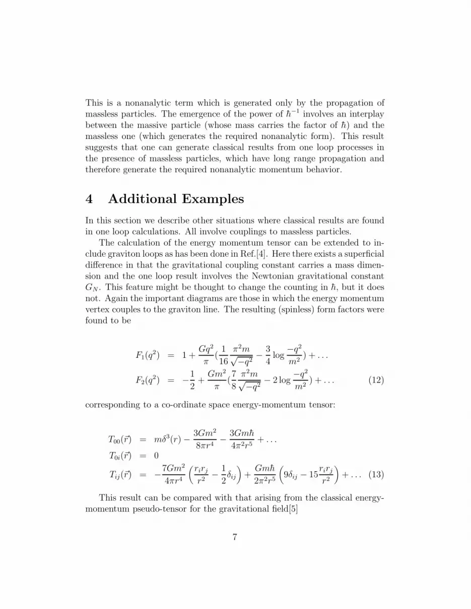
This result can be also be seen to arise via a simple one loop diagram, asshown in Figure 2. Again, for simplicity, we assume that both systems arespinless. The two-photon vertex associated with the electric polarizabilitycan be modelled in terms of a transition to a JP = 1− intermediate state (cf.Figure 2), yielding the Compton structure

AmpE =8π

mαE [ǫ1 · ǫ2P · k2P · k1 + ǫ1 · Pǫ2 · Pk1 · k2

− ǫ1 · Pǫ2 · k1P · k2 − ǫ2 · Pǫ1 · k2P · k1] (20)

where P = 12(p1 + p2) is the mean hadron four- momentum. One can also

include the magnetic polarizability via transition to a JP = 1+ intermediatestate, yielding

AmpB =8π

mαB [ǫ1 · ǫ2P · k2P · k1 + ǫ1 · Pǫ2 · Pk1 · k2

− ǫ1 · Pǫ2 · k1P · k2 − ǫ2 · Pǫ1 · k2P · k1

− k1 · k2ǫ1 · ǫ2P · P + ǫ1 · k2ǫ2 · k1P · P ] (21)

Calculating Figure 2 via standard methods, and keeping the nonanalyticpieces of the various Feynman triangle integrals, one finds the thresholdamplitude

Amp =e2q2m

4π

[

2αEπ2

√

M2

−q2+ (

11

3αE +

5

3βM )

]

(22)

where we have indicated the separate contributions from pole and seagull dia-grams. Including the normalization factor 1/4mM and Fourier transformingwe find the potential energy

V2γ(r) = −1

2

αemαE

r4+

αem(11αE + 5βM)h

Mr5+ ... (23)

9

1±

0+

0+

+ 1±

0+

0+

Figure 2: One loop diagrams used to model the interaction of a chargedparticle with a neutral polarizable system.

We see again that the one loop calculation has yielded the classical termaccompanied by quantum corrections. It should be noted here that, althoughwe have represented the two photon electric/magnetic polarizability couplingin terms of a simple contact interaction, as done by Bernabeu and Tarrach[6],the result is in complete agreement with a full box plus triangle diagramcalculation by Sucher and Feinberg[7].

There exist additional examples—a similar result obtains by consideringthe generation of an electric quadrupole moment by an external field gradient.Defining the field gradient via

Eij =1

2(∇iEj + ∇jEi)) (24)

and the quadrupole polarizability via

Qij = 4παE2Eij (25)

The classical energy due to interaction of this moment with the field gradientis given by

U = −1

2αE2EijEij (26)

The quadrupole polarizability can be modelled in terms of excitation to aJP = 2+ excited state and again, a simple one loop calculation finds a com-bination of classical and quantum terms. Similarly, in a gravitational analog,

10

the presence of a point mass produces a field gradient which generates a grav-itational quadrupole, which in turn interacts with the field gradient and leadsto a classical energy.

Finally, the gravitational potential between two heavy masses has beentreated to one loop in an effective field theory treatment of quantum gravity[8].Again, the diagrams involving two graviton propagators in a loop yield squareroot nonanalytic terms which reproduce the nonlinear classical corrections tothe potential which are predicted by general relativity[9]. This feature hasbeen known for some time[10].

5 A dispersive treatment

The lesson here is clear—these examples all involve one loop diagrams whichcontain a combination of classical and quantum mechanical effects, whereinthe classical piece is signaled by the presence of a square root nonanalytic-ity while the quantum component is associated with a ln−q2 term. Theseresults violate the usual expectation of the loop-h expansion. We can fur-ther understand the association of classical effects with massless particles bystudying a dispersive treatment. In this approach we can see directly thatthe classical terms are associated with the dispersion integral extending downto zero momentum, which is possible only if the particles in the associatedcut are massless.

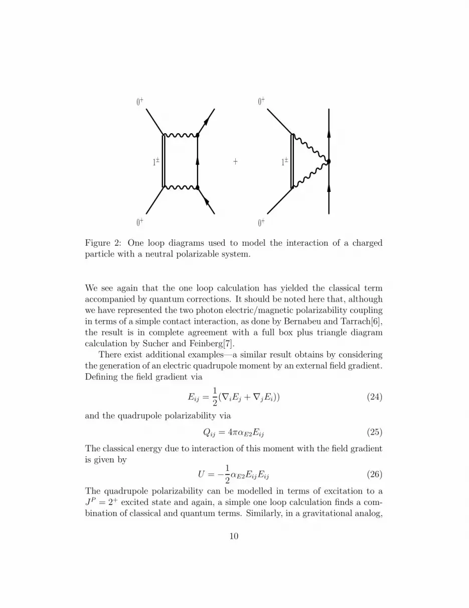
It is useful to use the Cutkosky rules to look at the absorptive componentof the triangle diagram shown in Figure 3, wherein we assume (temporarily)that the exchanged particles have mass µ. A simple calculation yields[11]

γ(q2) ≡ Abs∫

d4k

(2π)4

1

(k2 − µ2)((k − q)2 − µ2)((k − p)2 − M2)

=∫

d4k

(2π)4

(2πi)2δ(k2 − µ2)δ((k − q)2 − µ2)

(k2 − µ2)((k − q)2 − µ2)((k − p)2 − M2)(27)

where

γ(q2) =1

8π√

q2(4M2 − q2)tan−1

√

(q2 − 4µ2)(4M2 − q2)

q2 − 2µ2(28)

The corresponding dispersion integral is given by

Γ(q2) =1

π

∫

∞

4µ2

dtγ(t)

t − q2 − iǫ(29)

11

k

k − q

p − k

k

p − q

Figure 3: Generic triangle diagram used in dispersive analysis.

The argument of the arctangent vanishes at threshold and the dispersionintegral yields a form of no particular interest. On the other hand in thelimit µ → 0, the argument of the arctangent becomes infinite at thresholdand instead we write

γ(q2) =1

8π√

q2(4M2 − q2)

π

2− tan−1

√

√

√

√

q2

(4M2 − q2)

(30)

where we have separated the result into two components—the piece propor-tional to π/2, which arises from the on-shell (delta function) piece of themass M propagator and the remaining terms which arise from the principalvalue integration. The dispersion integral now begins at zero and yields alogarithmic result from pieces of γ(q2) which behave as a constant as q2 → 0,while square root pieces arise from terms in γ(q2) which behave as 1/

√q2

in the infrared limit. From Eq. 30 we see that the former—the quantumcomponent—arises from the principal value integration while the latter—theclassical component—is associated with the on- shell contributions to γ(q2).This is to be expected. A classical contribution should arise from the casewhere both initial/final and intermediate state particles are on shell andtherefore physical.

In the electromagnetic case, we can understand how such a classical termarises by writing the Maxwell equation as

12

Aµ =1

jµ

Since the inverse D’Alembertian corresponds to the photon propagator, wesee that components of the triangle integral involving the massive particlebeing on-shell leads to physical values of the charge density jµ and thereforeto physical values of the vector potential. Comparing with Eqn. 28 we seethat if µ 6= 0 then, there exists no possibility of a square root term andtherefore no way for classical physics to arise. Thus the existence of classicalpieces can be traced to the existence of two (or more!) massless propagatorsin the Feynman integration.

6 Conclusions

We have seen above that in the presence of at least two massless propagators,classical physics can arise from loop contributions, in apparent contradictionto the usual loop- h expansion arguments. The presence of classical correc-tions are associated with a specific nonanalytic term in momentum space.Using a dispersion integral the origin of this phenomenon has been tracedto the infrared behavior of the Feynman diagrams involved, which is altereddramatically when the threshold of the dispersion integration is allowed tovanish, as can occur when two or more massless propagators are present. Weconclude that the standard expectation that the loop expansion is equivalentto an h expansion is not valid in the presence of coupling to two or moremassless particles.

Acknowledgements

We thank A. Zee for comments on the manuscript. This work was supportedin part by the National Science Foundation under award PHY-02-44802.

References

[1] See, e.g., R.J. Rivers, Path Integral Methods in Quantum Field

Theory, Cambridge Univ. Press, New York (1987), sec. 4.6,L. H. Ryder, Quantum Field Theory, Cambridge Univ. Press, NewYork (1985), p. 327,

13

C. Itzykson and J.-B. Zuber, Quantum Field Theory, McGraw Hill,New York (1980), sec. 6-2-1.

[2] J.F. Donoghue, B.R. Holstein, B. Garbrecht, and T. Konstandin, “Quan-tum corrections to the Reissner-Nordstroem and Kerr-Newman met-rics,” Phys. Lett. B529, 132 (2002) [arXiv:hep-th/0112237].

[3] J.D. Jackson, Classical Electrodynamics, Wiley, New York (1962).

[4] N.E.J. Bjerrum-Bohr, J.F. Donoghue, and B.R. Holstein, ‘Quantumcorrections to the Schwarzschild and Kerr metrics,” Phys. Rev. D68,084005 (2003) [arxivhep-th/0211071].

[5] S. Weinberg, Gravitation and Cosmology, Wiley, New York (1972).

[6] J. Bernabeu and R. Tarrach, “Long Range Potentials And The Electro-magnetic Polarizabilities,” Ann. Phys. (NY) 102, 323 (1976).

[7] G. Feinberg and J. Sucher, Phys. Rev. A27, 1958 (1983).

[8] N. E. J. Bjerrum-Bohr, J. F. Donoghue and B. R. Holstein, ‘Quantumgravitational corrections to the nonrelativistic scattering potential oftwo masses,” Phys. Rev. D67, 084033 (2003) [arXiv:hep-th/0211072].

[9] J. F. Donoghue,“General Relativity As An Effective Field Theory:The Leading Quantum Corrections,” Phys. Rev. D50, 3874 (1994)[arXiv:gr-qc/9405057].I. B. Khriplovich and G. G. Kirilin, arXiv:gr-qc/0402018 and JETP 95,981 (2002) [arXiv:0207118].

[10] S. N. Gupta and S. F. Radford, ‘Quantum Field Theoretical Electro-magnetic And Gravitational Two Particle Potentials,” Phys. Rev. D21,2213 (1980).D. G. Boulware and S. Deser, ‘Classical General Relativity Derived FromQuantum Gravity,” Ann. Phys. (NY) 89, 193 (1975).

[11] S. Scherer, Adv. Nucl. Phys. 27, 277 (2003). [arXiv hep-ph/0210398].

14