arXiv:hep-th/0212267v3 22 May 2003 Classical and Quantum Nambu Mechanics Thomas Curtright * Department of Physics, University of Miami, Coral Gables, FL 33124-8046, USA Cosmas Zachos † High Energy Physics Division, Argonne National Laboratory, Argonne, IL 60439-4815, USA (Received 26 December 2002; Accepted 28 April 2003) The classical and quantum features of Nambu mechanics are analyzed and fundamental is- sues are resolved. The classical theory is reviewed and developed utilizing varied examples. The quantum theory is discussed in a parallel presentation, and illustrated with detailed specific cases. Quantization is carried out with standard Hilbert space methods. With the proper physical interpretation, obtained by allowing for different time scales on differ- ent invariant sectors of a theory, the resulting non-Abelian approach to quantum Nambu mechanics is shown to be fully consistent. PACS numbers: 02.30.Ik,11.30.Rd,11.25.Yb Contents 1. Introduction 2 2. Classical Theory 4 2.1. Phase-space geometry 4 2.2. Properties of the classical brackets 5 2.3. Illustrative classical examples 9 3. Quantum Theory 16 3.1. Properties of the quantum brackets 16 3.2. Illustrative quantum examples 26 3.3. Summary Table 39 4. Conclusions 40 Acknowledgments 41 A. Formal Division 41 References 43 * Electronic address: [email protected] † Electronic address: [email protected] Typeset by REVT E X

Welcome message from author
This document is posted to help you gain knowledge. Please leave a comment to let me know what you think about it! Share it to your friends and learn new things together.
Transcript
arX
iv:h
ep-t
h/02
1226
7v3
22
May
200
3
Classical and Quantum Nambu Mechanics
Thomas Curtright∗
Department of Physics, University of Miami, Coral Gables, FL 33124-8046, USA
Cosmas Zachos†
High Energy Physics Division, Argonne National Laboratory, Argonne, IL 60439-4815, USA(Received 26 December 2002; Accepted 28 April 2003)
The classical and quantum features of Nambu mechanics are analyzed and fundamental is-sues are resolved. The classical theory is reviewed and developed utilizing varied examples.The quantum theory is discussed in a parallel presentation, and illustrated with detailedspecific cases. Quantization is carried out with standard Hilbert space methods. Withthe proper physical interpretation, obtained by allowing for different time scales on differ-ent invariant sectors of a theory, the resulting non-Abelian approach to quantum Nambumechanics is shown to be fully consistent.
PACS numbers: 02.30.Ik,11.30.Rd,11.25.Yb
Contents
1. Introduction 2
2. Classical Theory 42.1. Phase-space geometry 42.2. Properties of the classical brackets 52.3. Illustrative classical examples 9
3. Quantum Theory 163.1. Properties of the quantum brackets 163.2. Illustrative quantum examples 263.3. Summary Table 39
4. Conclusions 40
Acknowledgments 41
A. Formal Division 41
References 43
∗Electronic address: [email protected]†Electronic address: [email protected]
Typeset by REVTEX
Curtright & Zachos Nambu Mechanics
1. INTRODUCTION
a. A brief historical overview Nambu [38] introduced an elegant generalization of the clas-sical Hamiltonian formalism by suggesting to supplant the Poisson Bracket (PB) with a 3- orn-linear, fully antisymmetric bracket, the Classical Nambu Bracket (CNB), a volume-element Ja-cobian determinant in a higher dimensional space. This bracket, involving a dynamical quantityand two or more “Hamiltonians”, provides the time-evolution of that quantity in a generalization ofHamilton’s equations of motion for selected physical systems. It was gradually realized [9, 12, 37]that Nambu Brackets in phase space describe the generic classical evolution of all systems withsufficiently many independent integrals of motion beyond those required for complete integrabilityof the systems. That is to say, all such “superintegrable systems” [45] are automatically describedby Nambu’s mechanics [16, 23], whether one chooses to take cognizance of this alternate expressionof their time development or not. This approach to time evolution for superintegrable systems issupplementary to the standard Hamiltonian dynamics evolution and provides additional tools foranalyzing such systems. The power of Nambu’s method is evident in a manifest and simultaneousaccounting of a maximal number of the symmetries of these systems, and in an efficient applicationof algebraic methods to yield results even without detailed knowledge of their specific dynamics.
As a bonus, the classical volume-preserving features of Nambu brackets suggest that they areuseful for membrane theory [35]. There are in the literature several persuasive but inconclusive ar-guments that Nambu brackets are a natural language for describing extended objects, for example:[2, 6, 7, 14, 18, 27, 31, 34, 36, 40, 46].
In his original paper [38], Nambu also introduced operator versions of his brackets as toolsto implement the quantization of his approach to mechanics. He enumerated various logicalpossibilities involving them, arguing that some structures were either inconsistent or uninteresting,but he did not advocate the position that the remaining possibilities were untenable: Quantizationwas left as an open issue.
Unfortunately, subsequent unwarranted insistence on algebraic structures ill-suited to the solu-tion of the relevant physics problems resulted in a widely held belief that quantization of Nambumechanics was problematic1, especially when that quantization was formulated as a one-parameterdeformation of classical structures. In marked contrast to this prevailing pessimism, several illus-trative superintegrable systems were quantized in [16] in a phase-space framework, both withoutand with the construction of Quantum Nambu Brackets (QNBs). However, the phase-spacequantization utilized there, while most appropriate for comparing quantum expressions with theirclassical limits, is still unfamiliar to many readers and will not be used in this paper. Here, thequantization of all systems will be carried out in a conventional Hilbert space operator formalism.
It turns out [16] that all perceived difficulties in quantizing Nambu mechanics may be tracedmathematically to the algebraic inconsistencies inherent in selecting constraints in a top-downapproach, with little regard to the correct phase-space structure which already provides full andconsistent answers, and with insufficient attention towards obtaining specific answers compati-ble with those produced in the quantized Hamiltonian description of these systems. Moreover,the physics underlying these perceived difficulties is simple, and involves only basic principles inquantum mechanics.
1 A few representative statements from the literature are: “Associated statistical mechanics and quantization areunlikely.” [19]; “A quantum generalization of these algebras is shown to be impossible.” and “ . . . the quantumanalog of Nambu mechanics does not exist.” [41]; “Usual approaches to quantization have failed to give anappropriate solution...” [17]; “...direct application of deformation quantization to Nambu-Poisson structures isnot possible.” [18]; “The quantization of Nambu bracket turns out to be a quite non-trivial problem.” [47]; “Thisproblem is still outstanding.” [44].
Phys Rev D 2 hep-th/0212267
Curtright & Zachos Nambu Mechanics
b. Evolution scales in quantum physics Some physicists might hold, without realizing it, theprejudice that continuous time evolution in quantum mechanics must always be formulated in-finitesimally as a derivation. Accordingly, they implicitly assume the instantaneous temporalchange in all dynamical variables is always given by nothing but a simple derivative, so that for allproducts of linear operators
d
dt(AB) =
(
d
dtA
)
B + A
(
d
dtB
)
. (1)
This assumption allows time development on physical Hilbert spaces to be expressed algebraicallyin terms of commutators with a Hamiltonian, since commutators are also derivations.2
[H,AB] = [H,A] B + A [H,B] . (2)
Evidently this approach leads to the simplest possible formalism. But is it really necessary tomake this assumption and follow this approach?
It is not. Time evolution can also be expressed algebraically using quantum Nambu brackets.These quantum brackets are defined as totally antisymmetrized multi-linear products of any numberof linear operators acting on Hilbert space. When QNBs are used to implement time evolutionin quantum mechanics, the result is usually not a derivation, but contains derivations entwinedwithin more elaborate structures (although there are some interesting special exceptions that aredescribed in the following).
This more general point of view towards time development can be arrived at just by realizinga physical idea. When a system has a number of conserved quantities, it is possible to partitionthe system’s Hilbert space into invariant sectors. Time evolution on those various sectors maythen be formulated using different time scales for the different sectors3 The resulting expression ofinstantaneous changes in time is then not a derivation, in general, when acting on the full Hilbertspace, and therefore is not given by a simple commutator. Remarkably, however, it often turnsout to be given compactly in terms of QNBs. Conversely, if QNBs are used to describe timedevelopment, they usually impose different time scales on different invariant sectors of a system[16].
Nevertheless, so long as the different time scales are implemented in such a way as to produceevolving phase differences between nondegenerate energy eigenstates, there is no loss of informationin this more general approach to time evolution. In the classical limit, this method is not reallydifferent from the usual Hamiltonian approach. A given classical trajectory has fixed values for allinvariants, and hence would have a fixed time scale in Nambu mechanics. Time development of anydynamical quantity along a single classical trajectory would therefore always be just a derivation,with no possibility of mixing time scales. Quantum mechanics, on the other hand, is more subtle,since the preparation of a state may yield a superposition of components from different invariantsectors. Such superpositions will, in general, involve multiple time scales in Nambu mechanics.
Technically, the various time scales arise in quantum Nambu mechanics as the entwined eigen-values of generalized Jordan spectral problems, where selected invariants of the model in questionappear as operators in the spectral equation. The resulting structure represents a new class ofeigenvalue problems for mathematical physics. Fortunately, solutions of this new class can be found
2 For simplicity we will assume, unless otherwise stated, that the operators have no explicit time dependence,although it is an elementary exercise to relax this assumption.
3 In fact, the choice of time variables in the different invariant sectors of a quantum theory is very broad. Theyneed not be just multiples of one another, but could have complicated functional dependencies, as discussed in[13] and [36]. The closest classical counter-part of this is found in the general method of analytic time, recentlyexploited so effectively in [11, 21].
Phys Rev D 3 hep-th/0212267
Curtright & Zachos Nambu Mechanics
using traditional methods. (All this is explained explicitly in the context of the first example of§3.2.)
c. Related studies in mathematics Algebras which involve multi-linear products have alsobeen considered at various times in the mathematical literature, partly as efforts to understand orgeneralize Jordan algebras [28, 29, 33] (cf. especially the “associator”), but more generally follow-ing Higgins’ study in the mid-1950s [8, 20, 26, 32]. This eventually culminated in the investigationsof certain cohomology questions, by Schlesinger and Stasheff [43], by Hanlon and Wachs [24], andby Azcarraga, Izquierdo, Perelomov, and Perez Bueno [4, 5, 6], that led to results most relevant toNambu’s work.
d. Summary of material to follow After a few motivational remarks on the geometry ofHamiltonian flows in phase-space, §2.1, we describe the most important features of classical Nambubrackets, §2.2, with emphasis on practical, algebraic, evaluation methods. We delve into severalexamples, §2.3, to gain physical insight for the classical theory.
We then give a parallel discussion of the quantum theory, §3.1, so far as algebraic features andmethods of evaluation are concerned. We define QNBs, as well as Generalized Jordan Products(GJPs) that naturally arise in conjunction with QNBs, when the latter are resolved into productsof commutators. We define derivators as measures of the failure of the Leibniz rule for QNBs,and discuss Jacobi and Fundamental identities in a quantum setting. Then we again turn tovarious examples, §3.2, to illustrate both the elegance and peculiarities of quantization. We dealwith essentially the same examples in both classical and quantum frameworks, as a means ofemphasizing the similarities and, more importantly, delineating the differences between CNBs andQNBs. The examples chosen are all models based on Lie symmetry algebras: so (3) = su (2),so (4) = su (2)× su (2), so (n), u (n), u (n)× u (m), and g × g.
We conclude by summarizing our results, and by suggesting some topics for further study.An Appendix discusses the formal solution of linear equations in Lie and Jordan algebras, withsuggestions for techniques to bypass the effects of divisors of zero.
A hurried reader may wish to consider only §2.1, §2.2 through Eqn(10), §2.3 through Eqn(35),§3.1 through Eqn(102), and §3.2 through Eqn(153). This abridged material contains our mainpoints.
2. CLASSICAL THEORY
We begin with a brief geometrical discussion of phase-space dynamics, to motivate the definitionof classical Nambu brackets. We then describe properties of CNBs, with emphasis on practicalevaluation methods, including various recursion relations among the brackets and simplificationsthat result from classical Lie symmetries being imposed on the entries in the bracket. We summa-rize the theory of the fundamental identity and explain its subsidiary role. We then go throughseveral examples to gain physical insight for the classical formalism. All the examples are basedon systems with Lie symmetries: so(3) = su (2), u(n), so(4) = su(2)× su(2), and g × g.
2.1. Phase-space geometry
A Hamiltonian system with N degrees of freedom is integrable in the Liouville sense if it hasN invariants in involution (globally defined and functionally independent), and superintegrable[45] if it has additional independent conservation laws up to a maximum total number of 2N − 1invariants. For a maximally superintegrable system, the total multi-linear cross product of the2N − 1 local phase-space gradients of the invariants (each such gradient being perpendicular to itscorresponding invariant isocline) is always locally tangent to the classical trajectory.
Phys Rev D 4 hep-th/0212267
Curtright & Zachos Nambu Mechanics
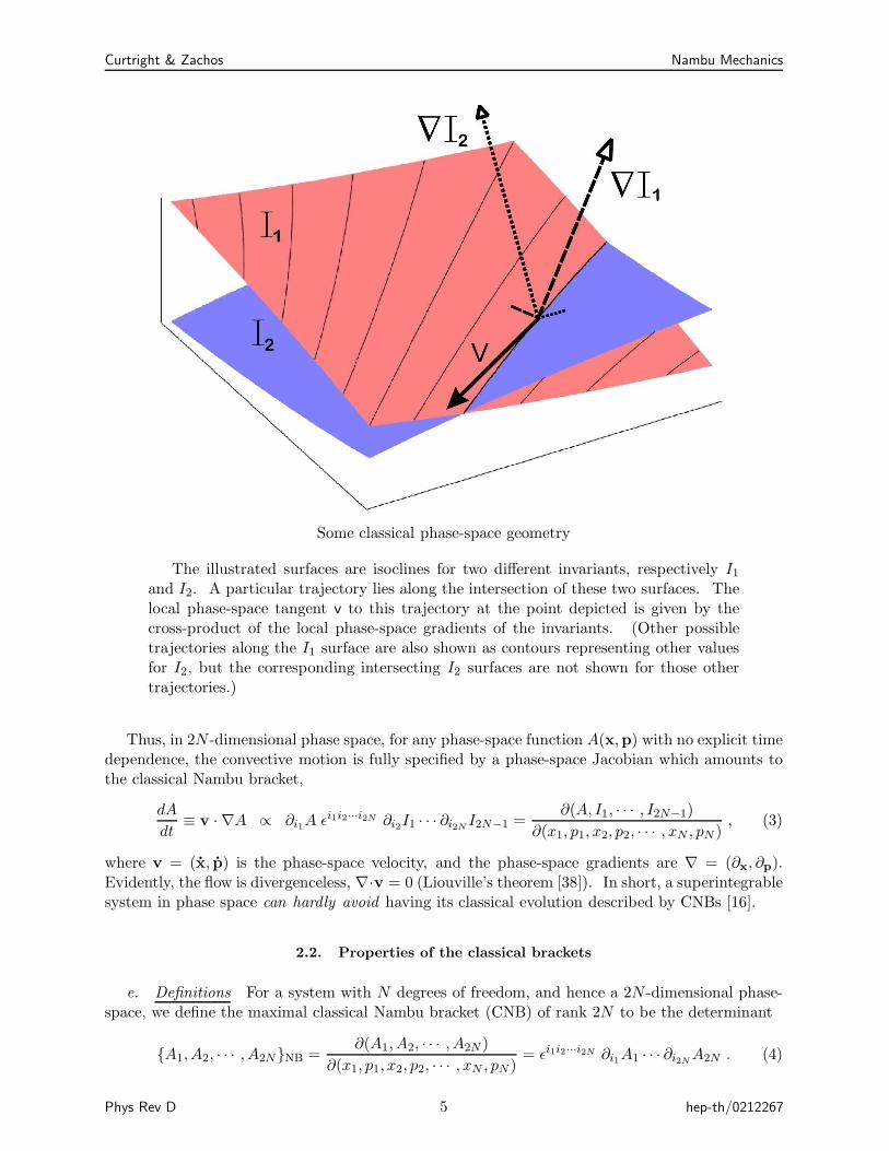
Some classical phase-space geometry
The illustrated surfaces are isoclines for two different invariants, respectively I1
and I2. A particular trajectory lies along the intersection of these two surfaces. Thelocal phase-space tangent v to this trajectory at the point depicted is given by thecross-product of the local phase-space gradients of the invariants. (Other possibletrajectories along the I1 surface are also shown as contours representing other valuesfor I2, but the corresponding intersecting I2 surfaces are not shown for those othertrajectories.)
Thus, in 2N -dimensional phase space, for any phase-space function A(x,p) with no explicit timedependence, the convective motion is fully specified by a phase-space Jacobian which amounts tothe classical Nambu bracket,
dA
dt≡ v · ∇A ∝ ∂i1A ǫi1i2···i2N ∂i2I1 · · · ∂i2N
I2N−1 =∂(A, I1, · · · , I2N−1)
∂(x1, p1, x2, p2, · · · , xN , pN ), (3)
where v = (x, p) is the phase-space velocity, and the phase-space gradients are ∇ = (∂x, ∂p).Evidently, the flow is divergenceless, ∇·v = 0 (Liouville’s theorem [38]). In short, a superintegrablesystem in phase space can hardly avoid having its classical evolution described by CNBs [16].
2.2. Properties of the classical brackets
e. Definitions For a system with N degrees of freedom, and hence a 2N -dimensional phase-space, we define the maximal classical Nambu bracket (CNB) of rank 2N to be the determinant
A1, A2, · · · , A2NNB =∂(A1, A2, · · · , A2N )
∂(x1, p1, x2, p2, · · · , xN , pN )= ǫi1i2···i2N ∂i1A1 · · · ∂i2N
A2N . (4)
Phys Rev D 5 hep-th/0212267
Curtright & Zachos Nambu Mechanics
This bracket is linear in its arguments, and completely antisymmetric in them. It may be thoughtof as the Jacobian induced by transforming to new phase space variables Ai, the “elements” in thebracket. As expected for such a Jacobian, two functionally dependent elements cause the bracketto collapse to zero. So, in particular, adding to any element an arbitrary linear combination ofthe other elements will not change the value of the bracket.
Odd dimensional brackets are also defined identically [38], in an odd-dimensional space.f. Recursion relations The simplest of these are immediate consequences of the properties of
the totally antisymmetric Levi-Civita symbols.
∂ (A1, A2, · · · , Ak)
∂ (z1, z2 · · · , zk)=
ǫi1···ik
(k − 1)!
(
∂A1
∂zi1
)
∂ (A2, · · · , Ak)
∂ (zi2 , · · · , zik)=
ǫj1···jk
(k − 1)!
(
∂Aj1
∂z1
)
∂ (Aj2 , · · · , Ajk)
∂ (z2, · · · , zk). (5)
However, these k = 1 + (k − 1) resolutions are not especially germane to a phase-space discussion,since they reduce even brackets into products of odd brackets.
More usefully, any maximal even rank CNB can also be resolved into products of Poissonbrackets. For example, for systems with two degrees of freedom, A,BPB = ∂(A,B)
∂(x1,p1)+ ∂(A,B)
∂(x2,p2),
and the 4-bracket A,B,C,DNB ≡∂(A,B,C,D)
∂(x1,p1,x2,p2)resolves as4
A,B,C,DNB = A,BPB C,DPB − A,CPB B,DPB − A,DPB C,BPB , (6)
in comportance with full antisymmetry under permutations of A,B,C, and D. The general resultfor maximal rank 2N brackets for systems with a 2N -dimensional phase-space is5
A1, A2, · · · , A2N−1, A2NNB =∑
all (2N)! permsσ1,σ2,··· ,σ2Nof the indices1,2,··· ,2N
sgn (σ)
2NN !Aσ1 , Aσ2PB Aσ3 , Aσ4PB · · ·
Aσ2N−1, Aσ2N
PB,
(7)
where sgn (σ) = (−1)π(σ) with π (σ) the parity of the permutation σ1, σ2, · · · , σ2N. The sumonly gives (2N − 1)!! = (2N)!/
(
2NN !)
distinct products of PBs on the RHS, not (2N)! Each suchdistinct product appears with net coefficient ±1.
The proof of the relation (7) is elementary. Both left- and right-hand sides of the expressionare sums of 2N -th degree monomials linear in the 2N first-order partial derivatives of each of theAs. Both sides are totally antisymmetric under permutations of the As. Hence, both sides arealso totally antisymmetric under interchanges of partial derivatives. Thus, the two sides must beproportional. The only issue left is the constant of proportionality. This is easily determined tobe 1, by comparing the coefficients of any given term appearing on both sides of the equation, e.g.∂x1A1∂p1A2 · · · ∂xN
A2N−1∂pNA2N .
For similar relations to hold for sub-maximal even rank Nambu brackets, these must first be de-fined. It is easiest to just define sub-maximal even rank CNBs by their Poisson bracket resolutions
4 These PB resolutions are somewhat simpler than their quantum counterparts, to be given below in §3.1, sinceordering of products is not an issue here.
5 This is essentially a special case of Laplace’s theorem on the general minor expansions of determinants (cf. Ch. 4in [1]), although it must be said that we have never seen it written, let alone used, in exactly this form, either intreatises on determinants or in textbooks on classical mechanics.
Phys Rev D 6 hep-th/0212267
Curtright & Zachos Nambu Mechanics
as in (7)6:
A1, A2, · · · , A2n−1, A2nNB =∑
(2n)! perms σ
sgn (σ)
2nn!Aσ1 , Aσ2PB Aσ3 , Aσ4PB · · ·
Aσ2n−1 , Aσn
PB,
(8)only here we allow n < N . So defined, these sub-maximal CNBs enter in further recursiveexpressions. For example, for systems with three or more degrees of freedom, A,BPB = ∂(A,B)
∂(x1,p1)+
∂(A,B)∂(x2,p2)
+ ∂(A,B)∂(x3,p3)
+ · · · , and a general 6-bracket expression resolves as
A1, A2, A3, A4, A5, A6NB = A1, A2PB A3, A4, A5, A6NB − A1, A3PB A2, A4, A5, A6NB
+ A1, A4PB A2, A3, A5, A6NB − A1, A5PB A2, A3, A4, A6NB
+ A1, A6PB A2, A3, A4, A5NB , (9)
with the 4-brackets resolvable into PBs as in (6). This permits the building-up of higher evenrank brackets proceeding from initial PBs involving all degrees of freedom. The general recursionrelation with this 2n = 2 + (2n− 2) form is
A1, A2, · · · , A2n−1, A2nNB = A1, A2PB A3, · · · , A2nNB
+
2n−1∑
j=3
(−1)j A1, AjPB A2, · · · , Aj−1, Aj+1, · · · , A2nNB
+ A1, A2nPB A2, · · · , A2n−1NB , (10)
and features 2n−1 terms on the RHS. This recursive result is equivalent to taking (8) as a definitionfor 2n < 2N elements, as can be seen by substituting the PB resolutions of the (2n− 2)-bracketson the RHS of (10). Similar relations obtain when the 2n elements in the CNB are partitionedinto sets of (2n− 2k) and 2k elements, with suitable antisymmetrization with respect to exchangesbetween the two sets.
These results may be extended beyond maximal CNBs to super-maximal brackets, in a usefulway. All such super-maximal classical brackets vanish, for the simple reason that there are notenough independent partial derivatives to avoid repeating columns of the implicit matrix whosedeterminant is under consideration. Another way to say this is as the impossibility to antisym-metrize more than 2N coordinate and momentum indices in 2N -dimensional phase space, so forany phase-space function V , we have ǫ[j1j2···j2N ∂i]V ≡ 0 , with ∂i = ∂/∂xi, ∂1+i = ∂/∂pi, 1 ≤ i(odd) ≤ 2N − 1. Consequently, ∂j1A1 · · · ∂j2N A2N ǫ[j1j2···j2N ∂i]V = 0, for any 2N phase-spacefunctions Aj, j = 1, · · · , 2N, and any V , a result that may be thought of as the vanishing of the(2N + 1)-th super-maximal CNB. As a further consequence, we have on 2N -dimensional phasespaces other super-maximal identities of the form
B1, · · · , Bk, V NBA1, A2, · · · , A2NNB = B1, · · · , Bk, A1NBV,A2, · · · , A2NNB (11)
+B1, · · · , Bk, A2NBA1, V,A3, · · · , A2NNB + · · ·+ B1, · · · , Bk, A2NNBA1, A2, · · · , A2N−1, V NB ,
for any choice of V , k, As, and Bs. We have distinguished here a (2N + 1)-th phase-space functionas V in anticipation of using the result later (cf. the discussion of the modified fundamental identity,(23) et seq.). The expansions in (8) and (10) also apply to the super-maximal case as well, wherethey provide vanishing theorems for the sums on the RHSs of those relations.
6 This definition is consistent with the classical limits of quantum ⋆-brackets presented and discussed in [16], fromwhich the same Poisson bracket resolutions follow as a consequence of taking the classical limit of ⋆-commutatorresolutions of even ⋆-brackets. It is also consistent with taking symplectic traces of maximal CNBs, again aspresented in [16] (see (14) to follow).
Phys Rev D 7 hep-th/0212267
Curtright & Zachos Nambu Mechanics
g. Reductions for classical Lie symmetries When the phase-space functions involved in aclassical bracket obey a Poisson bracket algebra (possibly even an infinite one), the NB reduces tobecome a sum of products, each product involving half as many phase-space functions (reductio addimidium). It follows as an elementary consequence of the PB resolution of even CNBs. For anyPB Lie algebra given by
Bi, BjPB =∑
m
c mij Bm , (12)
the PB resolution then gives (sum over all repeated ms is to be understood)
B1, · · · , B2k+1, ANB =∑
(2k+1)! perms σ
sgn (σ)
2kk!Bσ1 , Bσ2PB Bσ3 , Bσ4PB · · ·
Bσ2k−1, Bσ2k
PB
Bσ2k+1, A
PB
=∑
(2k+1)! perms σ
sgn (σ)
2kk!c m1σ1σ2
c m2σ3σ4
· · · c mkσ2k−1σ2k
Bm1Bm2 · · ·Bmk
Bσ2k+1, A
PB, (13)
where A is arbitrary. Of course, if A is also an element of the Lie algebra, then the last PB alsoreduces.
h. Traces Define the symplectic trace of a classical bracket as∑
i
xi, pi, A1, · · · , A2kNB = (N − k) A1, · · · , A2kNB . (14)
A complete reduction of maximal CNBs to PBs follows by inserting N − 1 conjugate pairs ofphase-space coordinates and summing over them.
A,BPB =1
(N − 1)!
A,B, xi1 , pi1 , · · · , xiN−1, piN−1
NB, (15)
where summation over all pairs of repeated indices is understood. Fewer traces lead to relationsbetween CNBs of maximal rank, 2N , and those of lesser rank, 2k.
A1, · · · , A2kNB =1
(N − k)!
A1, · · · , A2k, xi1 , pi1 , · · · , xiN−k, piN−k
NB. (16)
This is consistent with the PB resolutions (8) used to define the lower rank CNBs previously, andprovides another practical evaluation tool for these CNBs.
Through the use of such symplectic traces, Hamilton’s equations for a general system—notnecessarily superintegrable—admit an NB expression different from Nambu’s original one, namely
dA
dt= A,HPB =
1
(N − 1)!A,H, xi1 , pi1 , ..., xiN−1
, piN−1NB , (17)
where H is the system Hamiltonian.i. Derivations and the classical “Fundamental Identity” CNBs are all derivations with re-
spect to each of their arguments [38]. For even brackets, this follows from (4) for maximalCNBs, and from (8) (or (16)) for sub-maximal brackets.
δBA = A,B1, B2, · · · , B2n−1NB , (18)
where B is a short-hand for the string B1, B2, · · · , B2n−1. By derivation, we mean that Leibniz’selementary rule is satisfied,
δB(AA) = (δBA)A+ A (δBA) = A,B1, · · · , B2n−1NBA+ A A, B1, · · · , B2n−1NB . (19)
Phys Rev D 8 hep-th/0212267
Curtright & Zachos Nambu Mechanics
Moreover, when these derivations act on other maximal CNBs, they yield simple bracket identities[20, 38, 41],
δBC1, · · · , C2NNB = δBC1, · · · , C2NNB + · · ·+ C1, · · · , δBC2NNB , (20)
alternatively
C1, · · · , C2NNB, B1, · · · , B2n−1NB = C1, B1, · · · , B2n−1NB, · · · , C2NNB
+ · · ·+ C1, · · · , C2N , B1, · · · , B2n−1NBNB . (21)
In particular, any maximal CNB acting on any other maximal CNB always obeys the (4N − 1)-element, (2N + 1)-term identity [20, 41].
0 = A1, A2, · · · , A2NNB , B1, · · · , B2N−1NB−2N∑
j=1
A1, · · · , Aj , B1, · · · , B2N−1NB , · · · , A2N
NB.
(22)This has been designated “the Fundamental Identity” (FI) [44], although its essentially subsidiaryrole should be apparent in this classical context.
j. Invariant coefficients The fact that all CNBs are derivations, and that all super-maximalclassical brackets vanish, leads to a slightly modified form of 4N -element, (2N + 1)-term funda-mental identities, for a system in a 2N -dimensional phase-space [16].
B1, · · · , B2N−1, V A1, A2, · · · , A2NNBNB = V B1, · · · , B2N−1, A1NB , A2, · · · , A2NNB(23)
+ A1, V B1, · · · , B2N−1, A2NB , A3, · · · , A4N−1NB + · · ·+ A1, · · · , A2N−1, V B1, · · · , B2N−1, A2NNBNB ,
for any choice of V , As, and Bs. This identity is just the sum of the super-maximal identity (11), fork = 2N−1, plus V times the FI (22) for the derivation B1, · · · , B2N−1, A1, A2, · · · , A2NNBNB.
As a consequence of this modified FI, any proportionality constant V appearing in (3), i.e.
dA
dt= V A, I1, · · · , I2N−1NB , (24)
has to be a time-invariant if it has no explicit time dependence [23]. As proof [16], since the timederivation satisfies the conditions for the above δ, we have
d
dt(V A1, · · · , A2NNB) = V A1, · · · , A2NNB + V A1, · · · , A2NNB + · · ·+ V A1, · · · , A2NNB .
(25)Consistency with (24) requires this to be the same as
V V A1, · · · , A2NNB, I1, · · · , I2N−1NB = V A1, · · · , A2NNB (26)
+V V A1, I1, · · · , I2N−1NB, · · · , A2NNB + · · ·+ V A1, · · · , V A2N , I1, · · · , I2N−1NBNB .
By substitution of (23) with Bj ≡ Ij, V = 0 follows.
2.3. Illustrative classical examples
It is useful to consider explicit examples of classical dynamical systems described by Nambubrackets, to gain insight and develop intuition concerning CNBs. Previous classical examples weregiven by Nambu [38], and more recently, by Chatterjee [12], and by Gonera and Nutku [23, 39].We offer an eclectic selection based on those in [16].
Phys Rev D 9 hep-th/0212267
Curtright & Zachos Nambu Mechanics
k. SO(3) as a special case For example, consider a particle constrained to the surface of a
unit radius two-sphere S2, but otherwise moving freely. Three independent invariants of this maxi-mally superintegrable system are the angular momenta about the center of the sphere: Lx, Ly, Lz.Actually, no two of these are in involution, but this is quickly remedied, and moreover it is not ahindrance since in the Nambu approach to mechanics all invariants are on a more equal footing.
To be more explicit, we may coordinate the upper and lower (±) hemispheres by projecting theparticle’s location onto the equatorial disk,
(x, y) | x2 + y2 ≤ 1
. The invariants are then
Lz = xpy − ypx , Ly = ±√
1− x2 − y2 px , Lx = ∓√
1− x2 − y2 py . (27)
The last two are the de Sitter momenta, or nonlinearly realized axial charges corresponding to the“pions” x, y of this truncated σ-model.
The Poisson brackets of these expressions close into the expected SO(3) algebra,
Lx, LyPB = Lz , Ly, LzPB = Lx , Lz, LxPB = Ly . (28)
The usual Hamiltonian of the free particle system is the Casimir invariant [16]
H =1
2(LxLx + LyLy + LzLz) =
1
2
(
1− x2)
p2x +
1
2
(
1− y2)
p2y − xypxpy . (29)
Thus, it immediately follows algebraically that PBs of H with the L vanish, and their time-invariance holds.
d
dtL = L,HPB = 0 . (30)
So any one of the Ls and this Casimir constitute a pair of invariants in involution.The corresponding so (3) CNB dynamical evolution, found in [16], is untypically concise.
dA
dt= A,HPB = A,Lx, Ly, LzNB =
∂(A,Lx, Ly, Lz)
∂(x, px, y, py). (31)
The simplicity of this result actually extends to more general contexts, upon use of suitable linearcombinations. Special sums of such 4-brackets can be used to express time evolution for any classicalsystem with a continuous symmetry algebra underlying the dynamics and whose Hamiltonian isjust the quadratic Casimir of that symmetry algebra. The system need not be superintegrable, oreven integrable, in general.
Any simple Lie algebra allows a PB with a quadratic Casimir to be rewritten as a sum of4-brackets. Suppose
Qa, QbPB = fabcQc , (32)
in a basis where fabc is totally antisymmetric. Then, for the following linear combination of Nambu4-brackets weighted by the structure constants, use the PB resolution of the 4-bracket (6) to obtain(sum over repeated indices)
fabc A,Qa, Qb, QcNB = 3fabc A,QaPB Qb, QcPB = 3fabcfbcd A,QaPB Qd . (33)
Now, for simple Lie algebras (with appropriately normalized charges) one has
fabcfbcd = cadjoint δad , (34)
where cadjoint is a number (For example, cadjoint = N for su (N)). Thus the classical 4-bracketreduces to a PB with the Casimir QaQa,
fabc A,Qa, Qb, QcNB = 3 cadjoint A,QaPB Qa =3
2cadjoint A,QaQaPB , (35)
For su (2) = so (3), cadjoint = 2, fabc A,Qa, Qb, QcNB = 6 A,Lx, Ly, LzNB, and we establish (31)above.
Phys Rev D 10 hep-th/0212267
Curtright & Zachos Nambu Mechanics
l. U(n) and isotropic oscillators If we realize the U (n) algebra in the oscillator basis, wherethe phase-space “charges” Njk = (xj − ipj) (xk + ipk) /2 obey the PB relations
Njk, NlmPB = −i (Njmδkl −Nlkδjm) , j, k, l,m = 1, · · · , n , (36)
then the isotropic Hamiltonian is
H = ω
n∑
i=1
Ni , Ni ≡ Nii . (37)
This gives the n2 conservation laws
H,NijPB = 0 . (38)
However, only 2n − 1 of the Nij are functionally independent for a classical system with a 2n-dimensional phase-space. This follows because all full phase-space Jacobians (i.e., maximal CNBs)involving 2n of the Nij vanish. (For details, see the upcoming discussion surrounding (46).)
Following the logic that led to the previous reductio ad dimidium for general Lie symmetries,we obtain the main result for classical isotropic oscillator 2n-brackets.
m. Classical isotropic oscillator brackets (the U (n) reductio ad dimidium): Let N = N1 +N2 + · · · + Nn, and intercalate the n − 1 non-diagonal charges Ni i+1, for i = 1, · · · , n − 1, into aclassical Nambu 2n-bracket with the n mutually involutive Nj , for j = 1, · · · , n, to find7
A,N1, N12, N2, N23, · · · , Nn−1, Nn−1 n, NnNB = (−i)n−1 A,NPB N12N23 · · ·Nn−1 n
= (−i)n−1 AN12N23 · · ·Nn−1 n, NPB . (39)
This result follows from the U (n) PB algebra of the charges, (36). When the algebra is realizedspecifically by harmonic oscillators, the RHS factor may also be written as N12N23 · · ·Nn−1 n =(N2N3 · · ·Nn−1)N1 n.Proof: Linearity in each argument and total antisymmetry of the CNB allow us to replace anyone of the Ni by the sum N . Replace Nn → N , to obtain
A,N1, N12, N2, · · · , Nn−1, Nn−1 n, NnNB = A,N1, N12, N2, · · · , Nn−1, Nn−1 n, NNB . (40)
Now since N,NijPB = 0, the PB resolution of the 2n-bracket implies that N must appear“locked” in a PB with A, and therefore A cannot appear in any other PB. But then N1 is ininvolution with all the remaining free Nij except N12. So N1 must be locked in N1, N12PB.Continuing in this way, N2 must be locked in N2, N23PB, etc., until finally Nn−1 is locked inNn−1, Nn−1 nPB. Thus, all 2n entries have been paired and locked in the indicated n PBs, i.e.they are all “zipped-up”. Consequently,
A,N1, N12, N2, · · · , Nn−1, Nn−1 n, NnNB = A,NPB N1, N12PB · · · Nn−1, Nn−1 nPB . (41)
All the paired Njk Poisson brackets evaluate as Nj−1, Nj−1 jPB = −iNj−1 j, so
A,N1, N12, N2, · · · , Nn−1, Nn−1 n, NnNB = (−i)n−1 A,NPB N12 · · ·Nn−1 n . (42)
7 The non-diagonal charges are not real, but neither does this present a real problem. The proof leading to (39) alsogoes through if non-diagonal charges have their subscripts transposed. This allows replacing Ni i+1 with real orpurely imaginary combinations Ni i+1±Ni+1 i in the LHS 2n-bracket, to obtain the alternative linear combinationsNi i+1 ∓ Ni+1 i in the product on the RHS.
Phys Rev D 11 hep-th/0212267
Curtright & Zachos Nambu Mechanics
Finally, the PB with N may be performed either before or after the product of A with all theNj−1 j , since again N,NijPB = 0, and the PB is a derivation. Hence
A,NPB N12 · · ·Nn−1 n = AN12 · · ·Nn−1 n, NPB . QED (43)
Remarkably, in (39), the invariants which are in involution (i.e. the Cartan subalgebra of u (n))are separated out of the CNB into a single PB involving their sum (the Hamiltonian, H = ωN),while the invariants which are not in involution (n−1 of them, corresponding in number to the rankof SU (n)) are effectively swept into a simple product. Time evolution for the isotropic oscillatoris then given by [16]
(−i)n−1 N12 · · ·Nn−1 ndA
dt= ω A,N1, N12, N2, · · · , Nn−1, Nn−1 n, NnNB . (44)
This result reveals a possible degenerate situation for the Nambu approach.When any two or more of the phase-space gradients entering into the bracket are parallel, or
when one or more of them vanish, the corresponding bracket also vanishes, even if dAdt6= 0. Under
these conditions, the bracket does not give any temporal change of A: Such changes are “lost” bythe bracket. This can occur for the u (n) bracket under consideration whenever 0 = N12 · · ·Nn−1 n,i.e. whenever any Ni−1 i = 0 for some i. Initial classical configurations for which this is the caseare not evolved by this particular bracket. This is not really a serious problem, since on the onehand, the configurations for which it happens are so easily catalogued, and on the other hand, thereare other choices for the bracket entries which can be used to recover the lost temporal changes.It is just necessary to be aware of any such “kernel” when using any given bracket.
With that caveat in mind, there is another way to write (44) since the classical bracket is aderivation of each of its entries. Namely,
dA
dt= in−1ω A,N1, ln (N12) , N2, ln (N23) , N3, · · · , Nn−1, ln (Nn−1 n) , NnNB . (45)
The logarithms intercalated between the diagonal Njs on the RHS now have branch points corre-sponding to the classical bracket’s kernel.
The selection of 2n − 1 invariants to be used in the maximal U (n) bracket is not unique,of course. In the list that we have selected, the indices, 1, 2, · · · , n, can be replaced by anypermutation, σ1, σ2, · · · , σn, so long as the correlations between indices for elements in the listare maintained. That is, we may replace the elements N1, N12, N2, N23, · · · , Nn−1, Nn−1 n, Nn byNσ1 , Nσ1σ2 , Nσ2 , Nσ2σ3 , · · · , Nσn−1 , Nσn−1 σn , Nσn , and the reductio ad dimidium still holds.
A,Nσ1 , Nσ1σ2 , Nσ2 , Nσ2σ3 , · · · , Nσn−1 , Nσn−1 σn , Nσn
NB= (−i)n−1 A,NPB Nσ1σ2Nσ2σ3 · · ·Nσn−1 σn .
(46)Whatever list is selected, any invariant in that list is manifestly conserved by the 2n-bracket. Allother U (n) charges are also conserved by the bracket, even though they are not among the selectedlist of invariants. This last statement follows immediately from the A,HPB factor on the RHSof (46).
n. SO(n+1) and free particles on n-spheres For a particle moving freely on the surface of ann-sphere, Sn, one now has a choice of 2n − 1 of the n(n + 1)/2 invariant charges of so(n + 1),whose PB Lie algebra is conveniently written in terms of the n(n − 1)/2 rotation generators,Lab = xapb − xbpa, for a, b = 1, · · · , n, and in terms of the de Sitter momenta, Pa =
√
1− q2 pa,for a = 1, · · · , n, where q2 =
∑na=1 (xa)2. That PB algebra is
Pa, PbPB = Lab , Lab, PcPB = δacPb−δbcPa , Lab, LcdPB = Lacδbd−Ladδbc−Lbcδad+Lbdδac .(47)
Phys Rev D 12 hep-th/0212267
Curtright & Zachos Nambu Mechanics
By direct calculation, one of several possible expressions for time-evolution as a 2n-bracket is [16]
(−1)n−1 P2P3 · · ·Pn−1dA
dt=
∂ (A,P1, L12, P2, L23, P3, · · · , Pn−1, Ln−1 n, Pn)
∂ (x1, p1, x2, p2, · · · , xn, pn), (48)
where dAdt
= A,HPB and
H =1
2
n∑
a=1
PaPa +1
4
n∑
a,b=1
LabLab . (49)
The CNB expressing classical time-evolution may also be written, more compactly, as a derivation.
dA
dt= (−1)n−1 A,P1, L12, ln (P2) , L23, ln (P3) , · · · , ln (Pn−1) , Ln−1 n, PnNB . (50)
Once again, the branch points in the intercalated logarithms are indicators of this particularbracket’s kernel.
o. SO(4)=SU(2)×SU(2) as another special case The treatment of the 3-sphere S3 also ac-cords to the standard chiral model technology using left- and right-invariant Vielbeine [16]. Specif-ically, the two choices for such Dreibeine for the 3-sphere are [15]: q2 = x2 + y2 + z2
(±)V ia = ǫiabxb ±
√
1− q2 gai , (±)V ai = ǫiabxb ±√
1− q2 δai . (51)
The corresponding right and left conserved charges (left- and right-invariant, respectively) thenare
Ri = (+)V ia
d
dtxa = (+)V aipa , Li = (−)V i
a
d
dtxa = (−)V aipa . (52)
Perhaps more intuitive are the linear combinations into Axial and Isospin charges (again linear inthe momenta),
12 (R−L) =
√
1− q2 p ≡ A , 12 (R+L) = x× p ≡ I . (53)
It can easily be seen that the Ls and the Rs have PBs closing into the standard SU(2) × SU(2)algebra, i.e.
Li,LjNB = −2εijkLk , Ri,RjNB = −2εijkRk , Li,RjNB = 0 . (54)
Thus they are seen to be constant, since the Hamiltonian (and also the Lagrangian) can, in fact,be written in terms of either quadratic Casimir invariant,
H = 12L · L = 1
2R · R . (55)
The classical dynamics of this algebraic system is, like the single SU (2) invariant dynamics thatcomposes it, elegantly expressed on the six dimensional phase-space with maximal CNBs. We findvarious 6-bracket relations such as
∂ (A,H,R1,R2,L1,L2)
∂ (x1, p1, x2, p2, x3, p3)≡ A,H,R1,R2,L1,L2NB = −4L3R3
dA
dt, (56)
where 2H = R21 + R2
2 + R23 = L2
1 + L22 + L2
3, and A is an arbitrary function of the phase-spacedynamical variables. Also,
A,R1,R2,L3,L1,L2NB = −4R3dA
dt, (57)
Phys Rev D 13 hep-th/0212267
Curtright & Zachos Nambu Mechanics
and similarly (R←→ L)
A,R1,R2,R3,L1,L2NB = −4L3dA
dt. (58)
The kernels of these various brackets are evident from the factors multiplying dAdt
. None of theseparticular 6-bracket relations directly permits the L3 or R3 factors on their RHSs to be absorbedinto logarithms, through use of the Leibniz rule. But, by subtracting the last two to obtain
A,R1,R2,L3 −R3,L1,L2NB = 4 (L3 −R3)dA
dt, (59)
we can now introduce a logarithm to produce just a numerical factor multiplying the time derivative,
A,R1,R2, ln (L3 −R3)2 ,L1,L2
NB= 8
dA
dt. (60)
Similarly, by adding (57) and (58), we find
A,R1,R2, ln (L3 +R3)2 ,L1,L2
NB= −8
dA
dt. (61)
p. G×G chiral particles In general, the preceding discussion also applies to all chiral models,with the algebra g for a chiral group G replacing su(2). The Vielbein-momenta combinationsV ajpa represent algebra generator invariants, whose quadratic Casimir group invariants yield therespective Hamiltonians.
That is to say, for [10] group matrices U generated by exponentiated constant group algebramatrices T weighted by functions of the particle coordinates x, with U−1 = U †, we have
iU−1 d
dtU = (+)V j
a Tjd
dtxa = (+)V ajpaTj , iU
d
dtU−1 = (−)V ajpaTj , (62)
It follows that PBs of left- and right-invariant charges (designated by Rs and Ls, respectively), asdefined by the traces,
Rj ≡i
2tr
(
TjU−1 d
dtU
)
= (+)V ajpa , Lj ≡i
2tr
(
TjUd
dtU−1
)
= (−)V ajpa , (63)
close to the identical PB Lie algebras,
Ri,RjPB = −2fijkRk , Li,LjPB = −2fijkLk (64)
and PB commute with each other,
Ri,LjPB = 0 . (65)
These two statements are implicit in [10] and throughout the literature, and are explicitly provenin [16].
The Hamiltonian for a particle moving freely on the G×G group manifold is the simple form
H =1
2(paV
ai)(V bipb) , (66)
with either choice, V aj = (±)V aj . That is,
H = 12LjLj = 1
2RjRj , (67)
Phys Rev D 14 hep-th/0212267
Curtright & Zachos Nambu Mechanics
just as in the previous SO (4) = SU (2)×SU (2) case. There are now several ways to present timeevolution as CNBs for these models.
One way is as sums of 6-brackets. Making use of (34) and summing repeated indices:
fijkfimn A,H,Rj ,Rk,Lm,LnNB = fijkfimn Rj,RkPB Lm,LnPB A,HPB
= 4fijkfimnfjklfmnoRlLo A,HPB = 4c2adjointRlLl A,HPB . (68)
Thus we have
dA
dt=
1
4c2adjointRlLl
fijkfimn A,H,Rj ,Rk,Lm,LnNB . (69)
The bracket kernel here is given by zeroes of (Rl ± Ll)2 − 4H = ±2RlLl.
Another way to specify the time development for these chiral models is to use a maximal set ofinvariants in the CNB, selected from both left and right charges. Take n to be the dimension ofthe group G, then all charge indices range from 1 to n. For a point particle moving on the groupmanifold G × G, the maximal bracket involves 2n elements. So, for example, we have (note theranges of all the sums here are truncated to n− 1, as are the indices on the Levi-Civita symbols)
A,H,L1, · · · ,Ln−1,R1, · · · ,Rn−1NB
=1
[(n− 1)!]2
n−1∑
all i,j=1
εi1···in−1εj1···jn−1
A,H,Li1 , · · · ,Lin−1 ,Rj1, · · · ,Rjn−1
NB. (70)
The RHS here vanishes for even n, so we take odd n, say n = 1+2s. (To obtain a nontrivial resultfor even n, we may replace H by either Ln or Rn. We leave this as an exercise in the classicalcase. The relevant combinatorics are discussed later, in the context of the quantized model.) So,since H,LiPB = 0 = H,RiPB, by the PB resolution we can write
A,H,L1, · · · ,Ln−1,R1, · · · ,Rn−1NB (71)
= Kn
n−1∑
all i,j=1
εi1···in−1εj1···jn−1 A,HPB Li1 ,Li2PB · · ·
Lin−2 ,Lin−1
PBRj1,Rj2PB · · ·
Rjn−2 ,Rjn−1
PB,
where8
Kn=1+2s =1
4s (s!)2(72)
is a numerical combinatoric factor incorporating the number of equivalent ways to obtain the listof PBs in the product as written in (71).
Introducing a completely symmetric tensor, σk1···ks, defined by
σk1···ks =n−1∑
all i=1
εi1···in−1 fi1i2k1 · · · fin−2in−1ks, (73)
8 The number of ways of picking the n PBs in the formula (71), taking into account both ε’s, is (n − 2) (n − 4) · · · (1)×
(n − 2) (n − 4) · · · (1), so Kn =(
(n−2)(n−4)···(1)(n−1)!
)2
.
Phys Rev D 15 hep-th/0212267
Curtright & Zachos Nambu Mechanics
and using (64), we may rewrite (71) as (note the sums over ks and ms here are not truncated)
A,H,L1, · · · ,Ln−1,R1, · · · ,Rn−1NB
= (−2)n−1 Kn
n∑
all k,m=1
σk1···ksσm1···ms A,HPB Lk1 · · · LksRm1 · · · Rms . (74)
Thus we arrive at a maximal CNB expression of time evolution, for odd-dimensional G:
dA
dt= V A,H,L1, · · · ,Ln−1,R1, · · · ,Rn−1NB , (75)
where the invariant factor V on the RHS is given by
1
V=
1
(s!)2
n∑
all k=1
σk1···ksLk1 · · · Lks
n∑
all m=1
σm1···msRm1 · · · Rms , s ≡ n− 1
2. (76)
This factor determines the kernel of the bracket in question.All this extends in a straightforward way to even-dimensional groups G, and to the algebras of
symmetry groups involving arbitrary numbers of factors, G1 ×G2 × · · · .
3. QUANTUM THEORY
We now consider the quantization of Nambu mechanics. Despite contrary claims in the litera-ture, it turns out that the quantization is straightforward using the Hilbert space operator methodsas originally proposed by Nambu. All that is needed is a properly consistent physical interpreta-tion of the results, by allowing for dynamical time scales, as summarized in the Introduction. Weprovide a very detailed description of that interpretation in the following, but first we develop thetechniques and machinery that are used to reach and implement it. Our presentation parallels theprevious classical discussion as much as possible.
3.1. Properties of the quantum brackets
q. Definition of QNBs Define the quantum Nambu bracket, or QNB [38], as a fully antisym-metrized multilinear sum of operator products in an associative enveloping algebra,
[A1, A2, · · · , Ak] ≡∑
all k! perms σ1,σ2,··· ,σkof the indices 1,2,··· ,k
sgn (σ) Aσ1Aσ2 · · ·Aσk, (77)
where sgn (σ) = (−1)π(σ) with π (σ) the parity of the permutation σ1, σ2, · · · , σk. The bracketis unchanged by adding to any one element a linear combination of the others, in analogy with theusual row or column manipulations on determinants.
r. Recursion relations There are various ways to obtain QNBs recursively, from productsinvolving fewer operators. For example, a QNB involving k operators has both left- and right-sided resolutions of single operators multiplying QNBs of k − 1 operators.
[A1, A2, · · · , Ak] =∑
k! perms σ
sgn (σ)
(k − 1)!Aσ1 [Aσ2 , · · · , Aσk
]
=∑
k! perms σ
sgn (σ)
(k − 1)!
[
Aσ1 , · · · , Aσk−1
]
Aσk. (78)
Phys Rev D 16 hep-th/0212267
Curtright & Zachos Nambu Mechanics
On the RHS there are actually only k distinct products of single elements with (k − 1)-brackets,each such product having a net coefficient ±1. The denominator compensates for replication ofthese products in the sum over permutations. (We leave it as an elementary exercise for the readerto prove this result.)
For example, the 2-bracket is obviously just the commutator [A,B] = AB − BA, while the3-bracket may be written in either of two [38] or three convenient ways.
[A,B,C] = A [B,C] + B [C,A] + C [A,B]
= [A,B] C + [B,C]A + [C,A] B
= 32 [A,B] , C+ 1
2 [A,B , C]− [A, B,C] . (79)
Summing the first two lines gives anticommutators containing commutators on the RHS.
2 [A,B,C] = A, [B,C]+ B, [C,A]+ C, [A,B] . (80)
The last expression is to be contrasted to the Jacobi identity obtained by taking the difference ofthe first two RHS lines in (79).
0 = [A, [B,C]] + [B, [C,A]] + [C, [A,B]] . (81)
Similarly for the 4-bracket,
[A,B,C,D] = A [B,C,D]−B [C,D,A] + C [D,A,B]−D [A,B,C]
= − [B,C,D] A + [C,D,A] B − [D,A,B]C + [A,B,C]D . (82)
Summing these two lines gives
2 [A,B,C,D] = [A, [B,C,D]]− [B, [C,D,A]] + [C, [D,A,B]]− [D, [A,B,C]] , (83)
while taking the difference gives
0 = A, [B,C,D] − B, [C,D,A]+ C, [D,A,B] − D, [A,B,C] . (84)
There may be some temptation to think of the last of these as something like a generalization ofthe Jacobi identity, and, in principle, it is, but in a a crucially limited way, so that temptationshould be checked. The more appropriate and complete generalization of the Jacobi identity isgiven systematically below (cf. (119)).
s. Jordan products Define a fully symmetrized, generalized Jordan operator product (GJP).
A1, A2, · · · , Ak ≡∑
all k! perms σ1,σ2,··· ,σkof the indices 1,2,··· ,k
Aσ1Aσ2 · · ·Aσk, (85)
as introduced, in the bilinear form at least, by Jordan [29] to render non-Abelian algebras intoAbelian algebras at the expense of non-associativity. The generalization to multi-linears wassuggested by Kurosh [32], but the idea was not used in any previous physical application, as far aswe know. A GJP also has left- and right-sided recursions,
A1, A2, · · · , Ak =∑
k! perms σ
1
(k − 1)!Aσ1 Aσ2 , Aσ3 , · · · , Aσk
=∑
k! perms σ
1
(k − 1)!
Aσ2 , Aσ3 , · · · , Aσk−1
Aσk. (86)
Phys Rev D 17 hep-th/0212267
Curtright & Zachos Nambu Mechanics
On the RHS there are again only k distinct products of single elements with (k − 1)-GJPs, eachsuch product having a net coefficient +1. The denominator again compensates for replication ofthese products in the sum over permutations. (We leave it as another elementary exercise for thereader to prove this result.)
For example, a Jordan 2-product is obviously just an anticommutator A,B = AB + BA,while a 3-product is given by
A,B,C = A,BC + A,CB + B,CA= A B,C+ B A,C+ C A,B= 3
2 A,B , C+ 12 [[A,B] , C]− [A, [B,C]] . (87)
Equivalently, taking sums and differences, we obtain
2 A,B,C = A, B,C+ B, A,C+ C, A,B , (88)
as well as the companion of the Jacobi identity often encountered in super-algebras,
0 = [A, B,C] + [B, A,C] + [C, A,B] . (89)
Similarly for the 4-product,
A,B,C,D = A B,C,D+ B C,D,A + C D,A,B+ D A,B,C= A,B,CD + B,C,DA + C,D,AB + D,A,BC . (90)
Summing gives
2 A,B,C,D = A, B,C,D+ B, C,D,A+ C, D,A,B+ D, A,B,C , (91)
while subtracting gives
0 = [A, B,C,D] + [B, C,D,A] + [C, D,A,B] + [D, A,B,C] . (92)
Again the reader is warned off the temptation to think of the last of these as a bona fide general-ization of the super-Jacobi identity. While it is a valid identity, of course, following from nothingbut associativity, there is a superior and complete set of identities to be given later (cf. (119) tofollow).
t. (Anti)Commutator resolutions As in the classical case, Section 2.2, it is always possible toresolve even rank brackets into sums of commutator products, very usefully. For example,
[A,B,C,D] = [A,B] [C,D]− [A,C] [B,D]− [A,D] [C,B]
+ [C,D] [A,B]− [B,D] [A,C]− [C,B] [A,D] . (93)
An arbitrary even bracket of rank 2n breaks up into (2n)!/ (2n) = n! (2n − 1)!! such products.Another way to say this is that even QNBs can be written in terms of GJPs of commutators. Thegeneral result is
[A1, A2, · · · , A2n−1, A2n] =∑
(2n)! perms σ
sgn (σ)
2nn!
[Aσ1 , Aσ2 ] , [Aσ3 , Aσ4 ] , · · · ,[
Aσ2n−1 , Aσ2n
]
. (94)
An even GJP also resolves into symmetrized products of anticommutators.
A1, A2, · · · , A2n−1, A2n =∑
(2n)! perms σ
1
2nn!
Aσ1 , Aσ2 , Aσ3 , Aσ4 , · · · ,
Aσ2n−1 , Aσ2n
.
(95)
Phys Rev D 18 hep-th/0212267
Curtright & Zachos Nambu Mechanics
This resolution makes it transparent that all such even brackets will vanish if one or more of theAi are central (i.e. commute with all the other elements in the bracket). For instance, if any oneAi is a multiple of the unit operator, the 2n-bracket will vanish. (This same statement does notapply to odd brackets, as Nambu realized originally for 3-brackets [38], and consequently there areadditional hurdles to be overcome when using odd QNBs.)
As in the classical bracket formalism, the proofs of the (anti)commutator resolution relations areelementary. Both left- and right-hand sides of the expressions are sums of 2n-th degree monomialslinear in each of the As. Both sides are either totally antisymmetric, in the case of (94), ortotally symmetric, in the case of (95), under permutations of the As. Thus the two sides must beproportional. The only open issue is the constant of proportionality. This is easily determined tobe 1, just by comparing the coefficients of any given term appearing on both sides of the equation,e.g. A1A2 · · ·A2N−1A2N .
It is clear from the commutator resolution of even QNBs that totally symmetrized GJPs andtotally antisymmetrized QNBs are not unrelated. In fact, the relationship is most pronounced inquantum mechanical applications where the operators form a Lie algebra.
u. Reductions for Lie algebras In full analogy to the classical case above, when the operatorsinvolved in a QNB close into a Lie algebra, even if an infinite one, the Nambu bracket reducesin rank to become a sum of GJPs involving about half as many operators (quantum reductio addimidium). It follows as an elementary consequence of the commutator resolution of the Nambubracket. First, consider even brackets, since the commutator reduction applies directly to thatcase. From the commutator resolution, it follows that for any Lie algebra given by
[Bi, Bj ] = i~∑
m
c mij Bm , (96)
we have for arbitrary A (sum over repeated ms)9
[B1, · · · , B2k+1, A] =∑
(2k+1)! perms σ
sgn (σ)
2kk!
[Bσ1 , Bσ2 ] , [Bσ3 , Bσ4 ] , · · · ,[
Bσ2k−1, Bσ2k
]
,[
Bσ2k+1, A]
=∑
(2k+1)! perms σ
sgn (σ)
2kk!(i~)k c m1
σ1σ2c m2σ3σ4
· · · c mkσ2k−1σ2k
Bm1 , Bm2 , · · · , Bmk,[
Bσ2k+1, A]
.
(97)
For odd brackets, it is first necessary to resolve the QNB into products of single operators witheven brackets, and then resolve the various even brackets into commutators. This gives a largersum of terms for odd brackets, but again each term involves about half as many Jordan productscompared to the number of commutators resolving the original Nambu bracket. The mixture ofalgebraic structures in (97) suggests referring to this as a Nambu-Jordan-Lie (NJL) algebra.
v. The classical limit Since Poisson brackets are straightforward classical limits of commuta-tors,
lim~→0
(
1
i~
)
[A,B] = A,BPB ,
it follows that the commutator resolution of all even QNBs directly specifies their classical limit.(For a detailed approach to the classical limit, including sub-dominant terms of higher order in ~,see, e.g., the Moyal Bracket discussion in [16].)
9 After obtaining this result, and using it in [16], we learned that similar statements appeared previously in [5, 6].
Phys Rev D 19 hep-th/0212267
Curtright & Zachos Nambu Mechanics
For example, from
[A,B,C,D] = [A,B] , [C,D] − [A,C] , [B,D] − [A,D] , [C,B] , (98)
with due attention to a critical factor of 2 (i.e. the anticommutators on the RHS become just twicethe ordinary products of their entries), the classical limit emerges as
1
2lim~→0
(
1
i~
)2
[A,B,C,D] = A,BPB C,DPB − A,CPB B,DPB − A,DPB C,BPB
= A,B,C,DNB . (99)
And so it goes with all other even rank Nambu brackets. For a 2n-bracket, one sees that
1
n!lim~→0
(
1
i~
)n
[A1, A2, · · · , A2n] =∑
(2n)! perms σ
sgn (σ)
2nn!Aσ1 , Aσ2PB Aσ3 , Aσ4PB · · ·
Aσ2n−1 , Aσ2n
PB
= A1, A2, · · · , A2nNB . (100)
This is another way to establish that there are indeed (2n− 1)!! independent products of n Poissonbrackets summing up to give the PB resolution of the classical Nambu 2n-bracket. Once againdue attention must be given to a critical additional factor of n! (as in the denominator on the LHSof (100)) since the GJPs on the RHS of (94) will, in the classical limit, always replicate the sameclassical product n! times.
w. The Leibniz rule failure and derivators Define the derivator to measure the failure of thesimplest Leibniz rule for QNBs,
k+1∆B (A,A) ≡ (A,A |B1, · · · , Bk) ≡ [AA , B1, · · · , Bk]−A [A, B1, · · · , Bk]− [A,B1, · · · , Bk]A .(101)
The first term on the RHS is a (k + 1)-bracket acting on just the product of A and A, the orderof the bracket being evident in the pre-superscript of the ∆B notation. This reads in an obviousway. For instance, 4∆B is a “4-delta of Bs”. That notation also emphasizes that the Bs act onthe pair of As. The second notation in (101) makes explicit all the Bs and is useful for computercode.
Any ∆B acts on all pairs of elements in the enveloping algebra A to produce another elementin A.
∆B : A× A 7−→ A . (102)
When ∆B does not vanish the corresponding bracket with the Bs does not define a derivation onA. The derivator ∆B (A,A) is linear in both A and A, as well as linear in each of the Bs.
Less trivially, from explicit calculations, we find inhomogeneous recursion relations for thesederivators.
(A,A |B1, · · · , Bk) =1
2
∑
k! perms σ
sgn (σ)
(k − 1)!
(
(
A,A |Bσ1 , · · · , Bσk−1
)
Bσk+ (−1)k Bσk
(
A,A |Bσ1 , · · · , Bσk−1
)
)
+1
2
∑
k! perms σ
sgn (σ)
(k − 1)!
(
[A,Bσk][
Bσ1 , · · · , Bσk−1,A]
−[
A,Bσ1 , · · · , Bσk−1
]
[Bσk,A]
)
+(−1)k+1 − 1
2A [B1, · · · , Bk]A. (103)
Phys Rev D 20 hep-th/0212267
Curtright & Zachos Nambu Mechanics
Alternatively, we may write this so as to emphasize the number of distinct terms on the RHS anddistinguish between the even and odd bracket cases. The first two terms under the sum on theRHS give a commutator/anticommutator for k odd/even, and the last term is absent for k odd.
For even (2n+2)-brackets, this becomes
2 (A,A |B1, · · · , B2n+1) = [(A,A |B1, · · · , B2n) , B2n+1]
+ [A,B2n+1] [B1, · · · , B2n,A]− [A,B1, · · · , B2n] [B2n+1,A]
+ (2n signed permutations of the Bs) , (104)
where the first RHS line involves derivators of reduced rank, within commutators. For odd (2n+1)-brackets, it becomes
2 (A,A |B1, · · · , B2n) = (A,A |B1, · · · , B2n−1) , B2n+ [A,B2n] [B1, · · · , B2n−1,A]− [A,B1, · · · , B2n−1] [B2n,A]
+ (2n-1 signed permutations of the Bs)
− 2A [B1, · · · , B2n]A , (105)
where the first RHS line involves derivators of reduced rank, within anticommutators. Note theadditional inhomogeneity in the last RHS line of these results. It may be viewed as a type ofquantum obstruction in the recursion relation for the odd (2n+1)-bracket.
The obstruction is clarified when we specialize to n = 1, i.e. the 3-bracket case. Sincecommutators are always derivations, one has 2∆B (A,A) = 0, and the first RHS line vanishes in(105) for the 3∆B (A,A) case. So we have just
(A,A |B1, B2) = [A,B2] [B1,A]− [A,B1] [B2,A]−A [B1, B2]A . (106)
The first two terms on the RHS are O(
~2)
while the last is O (~). It is precisely this last termwhich was responsible for some of Nambu’s misgivings concerning his quantum 3-bracket. Inparticular, even in the extreme case when both A and A commute with the Bs, 3∆B (A,A) doesnot vanish:
(A,A |B1, B2)|[A,Bi]=0=[A,Bi]= −AA [B1, B2] . (107)
By contrast, for the even (2n+2)-bracket, all terms on the RHS of (104) are generically of thesame order, O
(
~n+1)
, and all terms vanish if A and A commute with all the Bs. In terms ofcombinatorics, this seems to be the only feature for the simple, possibly failed, Leibniz rule thatdistinguishes between even and odd brackets. An even-odd QNB dichotomy has been previouslynoted [24] and stressed [6], for other reasons.
The size of the brackets involved in the derivators can be reduced when the operators obey aLie algebra as in (96). The simplest situation occurs when the bracket is even. For this situationwe have
(A,A |B1, · · · , B2k+1) =∑
(2k+1)! perms σ
sgn (σ)
2kk!(i~)k c m1
σ1σ2c m2σ3σ4
· · · c mkσ2k−1σ2k
× (108)
×(
Bm1 , · · · , Bmk,[
Bσ2k+1, AA
]
−A
Bm1 , · · · , Bmk,[
Bσ2k+1,A]
−
Bm1 , · · · , Bmk,[
Bσ2k+1, A]
A) .
x. Generalized Jacobi identities and QFIs We previously pointed out some elementary iden-tities involving QNBs, e.g. (84) and (92), which are suggestive of generalizations of the Jacobiidentity for commutators. Those particular identities, while true, were not designated as “gener-alized Jacobi identities” (GJIs), for the simple fact that they do not involve the case where QNBs
Phys Rev D 21 hep-th/0212267
Curtright & Zachos Nambu Mechanics
of a given rank act on QNBs of the same rank. Here, we explore QNB identities of the latter type.There are indeed acceptable generalizations of the usual commutators-acting-on-commutators Ja-cobi identity (i.e. quantum 2-brackets acting on quantum 2-brackets), and these generalizationsare indeed valid for all higher rank QNBs (i.e. quantum n-brackets acting on quantum n-brackets).However, there is an essential distinction to be drawn between the even and odd quantum bracketcases [6, 24].
It is important to note that, historically, there have been some incorrect guesses and false startsin this direction that originated from the so-called fundamental identity obeyed by classical Nambubrackets, (22). This simple identity apparently misled several investigators [41], most recently [44]and [17, 18], to think of it as a “fundamental” generalization of the Jacobi identity, without takingcare to preserve the Jacobi Identity’s traditional role of encoding nothing but associativity. Thesesame investigators then insisted that a “correct quantization” of the classical Nambu bracket mustsatisfy an identity of the same form as (22).
Unfortunately for them, QNBs do not satisfy this particular identity, in general, and therebypose a formidable problem to proponents of that identity’s fundamental significance. This difficultyled [44] and [17, 18], to seek alternative ways to quantize CNBs, ultimately culminating in the so-called Abelian deformation method [17, 18]. This amounted to demanding that the quantizedbrackets satisfy the mathematical postulates of an “n-Lie algebra” as defined by Filippov [20]many years earlier. However, not only are those postulates not satisfied by generic QNBs, butmore importantly, those postulates are not warranted by the physics of QNBs, as will be clear inthe examples to follow.
The correct generalizations of the Jacobi identities which do encode associativity were foundindependently by groups of mathematicians [24] and physicists [4, 6]. Interestingly, both groupswere studying cohomology questions, so perhaps it is not surprising that they arrived at the sameresult. (Fortunately for us the result is sufficiently simple in its combinatorics that we do notneed to go through the cohomology issues.) The acceptable generalization of the Jacobi identitythat was found is satisfied by all QNBs, although for odd QNBs there is a significant differencein the form of the final result: It contains an “inhomogeneity”. The correct generalization isobtained just by totally antisymmetrizing the action of one n-bracket on the other. Effectively,this amounts to antisymmetrizing the form of the RHS of (22) over all permutations of the As andBs, including all exchanges of As with Bs.
We illustrate the correct quantum identity for the case of a 3-bracket acting on a 3-bracket,where the classical result is
0 = A,B,CNB ,D,ENB−A,D,ENB , B,C
NB−A, B,D,ENB , C
NB−A,B, C,D,ENBNB
,(109)
i.e. (22) for n = 3. For ease in writing, we let A1 ≡ A, A2 ≡ B, A3 ≡ C, B1 ≡ D, and B2 ≡ E.Consider [[A,B,C] ,D,E]. This QNB corresponds to the first term on the RHS of (109). If weantisymmetrize [[A,B,C] ,D,E] over all 5! permutations of A,B,C,D, and E, we obtain, with acommon overall coefficient of 12 = 2!3!, a total of 10 = 5!/ (2!3!) distinct terms as follows:
[[A,B,C] ,D,E] + [[A,D,E] , B,C] + [[D,B,E] , A,C] + [[D,E,C] , A,B]
− [[D,B,C] , A,E] − [[E,B,C] ,D,A]− [[A,D,C] , B,E]
− [[A,E,C] ,D,B]− [[A,B,D] , C,E] − [[A,B,E] ,D,C] . (110)
Now we determine the coefficient of any given monomial produced by this sum10. Since theexpression is totally antisymmetrized in all the five elements, the result must be proportional to
10 This line of argument is an adaptation of that in [24]. Equivalent methods are used in [4, 6].
Phys Rev D 22 hep-th/0212267
Curtright & Zachos Nambu Mechanics
[A,B,C,D,E]. To determine the constant of proportionality it suffices to consider the monomialABCDE. This particular monomial can be found in only 3 terms out of the ten in (110), namelyin
[[A,B,C] ,D,E] , [A, [B,C,D] , E] = − [[D,B,C] , A,E] , and [A,B, [C,D,E]] = [[D,E,C] , A,B] .(111)
The various terms are obtained just by “shifting” the interior brackets from left to right within theexterior brackets, while keeping all the bracket entries in a fixed left-to-right order, and keepingtrack of the sgn (σ) factors. (Call this the “shifting bracket argument”.) The monomial ABCDEappears in each of these terms with coefficient +1, for a total of +3×ABCDE. Thus, we concludewith a 5-element, 11-term identity,
[[A,B,C] ,D,E] + [[A,D,E] , B,C] + [[D,B,E] , A,C] + [[D,E,C] , A,B]
− [[D,B,C] , A,E] − [[E,B,C] ,D,A]− [[A,D,C] , B,E]
− [[A,E,C] ,D,B]− [[A,B,D] , C,E] − [[A,B,E] ,D,C]
= 3 [A,B,C,D,E] . (112)
This is the prototypical generalization of the Jacobi identity for odd QNBs, and like the Jacobiidentity, it is antisymmetric in all of its elements. The RHS here is the previously designatedinhomogeneity.
The totally antisymmetrized action of odd n QNBs on other odd n QNBs results in(2n− 1)-brackets.
We recognize in the first line of (112) those QNB combinations which correspond to all four ofthe individual terms on the RHS of (109). However, the signs are changed for 3 of the 4 QNB termsrelative to those in (109). One might hope that changing these signs in the QNB combinationswill lead to some simplification, and indeed it does, but it does not cause the resulting expressionto vanish, as it did in (109). To see this, consider in the same way the effects of antisymmetrizingthe QNBs corresponding to each of the other three terms on the RHS of (109). The second RHSterm would have as correspondent − [[A,D,E] , B,C], which, when totally antisymmetrized, givesan overall common coefficient of 2!3! multiplying
− [[A,D,E] , B,C]− [[A,B,C] ,D,E]− [[B,D,C] , A,E] − [[B,C,E] , A,D]
+ [[B,D,E] , A,C] + [[C,D,E] , B,A] + [[A,B,E] ,D,C]
+ [[A,C,E] , B,D] + [[A,D,B] , E,C] + [[A,D,C] , B,E]
= −3 [A,B,C,D,E] . (113)
The third RHS term of (109) would have as correspondent − [A, [B,D,E] , C] = [[B,D,E] , A,C],which, when totally antisymmetrized, gives an overall common coefficient of 2!3! multiplying
[[B,D,E] , A,C] + [[B,A,C] ,D,E] + [[A,D,C] , B,E] + [[A,C,E] , B,D]
− [[A,D,E] , B,C]− [[C,D,E] , A,B]− [[B,A,E] ,D,C]
− [[B,C,E] , A,D]− [[B,D,A] , E,C]− [[B,D,C] , A,E]
= −3 [A,B,C,D,E] . (114)
The fourth and final RHS term of (109) would have as correspondent − [A,B, [C,D,E]] =[[C,D,E] , B,A], which, when totally antisymmetrized, gives an overall common coefficient of 2!3!
Phys Rev D 23 hep-th/0212267
Curtright & Zachos Nambu Mechanics
multiplying
[[C,D,E] , B,A] + [[C,B,A] ,D,E] + [[B,D,A] , C,E] + [[B,A,E] , C,D]
− [[B,D,E] , C,A] − [[A,D,E] , B,C]− [[C,B,E] ,D,A]
− [[C,A,E] , B,D]− [[C,D,B] , E,A] − [[C,D,A] , B,E]
= −3 [A,B,C,D,E] . (115)
Adding (110), (113), (114), and (115) leads to the sum of QNB combinations that corresponds tothe antisymmetrized form of the RHS of (109), namely
( [[A,B,C] ,D,E]− [[A,D,E] , B,C]− [A, [B,D,E] , C]− [A,B, [C,D,E]] )
±(nine distinct permutations of all four terms) = −6 [A,B,C,D,E] . (116)
This result shows that the simple combination of QNB terms that corresponds to (109) (withoutfull antisymmetrization) cannot possibly vanish unless the 5-bracket [A,B,C,D,E] vanishes.
A similar consideration of the action of a 4-bracket on a 4-bracket illustrates the general formof the GJI for even brackets and shows the essential differences between the even and odd bracketcases. We proceed as above by starting with the combination [[A,B,C,D] , E, F,G] , and thentotally antisymmetrizing with respect to A,B,C,D,E, F, and G. We find 35 = 7!/ (3!4!) distinctterms in the resulting sum. Now we determine the coefficient of any given monomial that wouldappear in this sum. Since the expression is again totally antisymmetrized in all the seven elements,the result must be proportional to [A,B,C,D,E, F,G]. To determine the constant of proportion-ality it suffices to consider the monomial ABCDEFG and use the shifting bracket argument, whichshows that this particular monomial can be found in only 4 terms out of the 35 in the sum, namelyin
[[A,B,C,D] , E, F,G] , − [A, [B,C,D,E] , F,G] , [A,B, [C,D,E,F ] , G] , and −[A,B,C, [D,E,F,G]] .(117)
The monomial ABCDEFG appears in these 4 terms with coefficients +1,−1,+1, and −1, for atotal of 0×ABCDEFG. Thus we conclude that ([4, 24], and also [6], especially Eqn(32))
[[A,B,C,D] , E, F,G] ± (34 distinct permutations) = 0 . (118)
This is the prototypical generalization of the Jacobi identity for even QNBs, and constitutes thefull antisymmetrization of all arguments of the analogous FI. There is no RHS inhomogeneity inthis case.
The totally antisymmetrized action of even n QNBs on other even n QNBs results in zero.
The generalized Jacobi identity for arbitrary n-brackets follows from the same simple analysisof coefficients of any given monomial, as in (111) and (117). The shifting bracket argumentactually leads to a larger set of results, where the action of any bracket on any other is totallyantisymmetrized. We present that larger generalization here, calling it the quantum Jacobi identity,or QJI. The GJI is the QJI for k = n− 1.
y. QJIs for QNBs
∑
(n+k)! perms σ
sgn (σ)[
[Aσ1 , · · · , Aσn ] , Aσn+1 , · · · , Aσn+k
]
= [A1, · · · , An+k]× n!k!×
(k + 1) if n is odd12
(
1 + (−1)k)
if n is even. (119)
Phys Rev D 24 hep-th/0212267
Curtright & Zachos Nambu Mechanics
This result is proven just by computing the coefficient of the A1 · · ·An+k monomial using theshifting bracket argument as given previously to establish (111) and (117). Other argumentsleading to the same result may be found in [4, 6].
This is the quantum identity that most closely corresponds to the general classical result (seethe second talk under [16], Eqn (28)) for any even n and any odd k (only n = 2N, k = 2N − 1 isthe FI),
A1, A2, · · · , AnNB , B1, · · · , BkNB−
n∑
j=1
A1, · · · , Aj , B1, · · · , BkNB , · · · , An
NB
= B1, B2, · · · , BkNB , A1, · · · , AnNB− · · ·+ Bk, B1, · · · , Bk−1NB , A1, · · · , AnNB
.(120)
While this classical identity holds without requiring full antisymmetrization over all exchangesof As and Bs, in contrast the quantum identity must be totally antisymmetrized if it is to be aconsequence of only the associativity of the underlying algebra of Hilbert space operators. Notethat the n!k! on the RHS of (119) may be replaced by just 1 if we sum only over permutationsin which the Ai≤n are interchanged with the Ai>n in
[
[Aσ1 , · · · , Aσn ] , Aσn+1 , · · · , Aσn+k
]
, andignore all permutations of the A1, A2, · · · , An among themselves, and of the An+1, · · · , An+k amongthemselves.
There is an important specialization of the QJI result [4, 24]: For any even n and any odd k
∑
(n+k)! perms σ
sgn (σ)[
[Aσ1 , · · · , Aσn ] , Aσn+1 , · · · , Aσn+k
]
= 0 . (121)
In particular, when k = n−1, for n even, the vanishing RHS obtains. All other n-not-even and/ork-not-odd cases of the QJI have the [A1, · · · , An+k] inhomogeneity on the RHS.
The QJI also permits us to give the correct form of the so-called fundamental identities validfor all QNBs. We accordingly call these quantum fundamental identities (QFIs), and present themin their general form.
z. QFIs for QNBs
∑
(n+k)! perms σ
sgn (σ) ([
[Aσ1 , · · · , Aσn ] , Aσn+1 , · · · , Aσn+k
]
−n∑
j=1
[
Aσ1 , · · · ,[
Aσj, Aσn+1 , · · · , Aσn+k
]
, · · · , Aσn
]
)
= [A1, · · · , An+k]× n!k!×
0 if k is odd(1− n) (k + 1) if k is even and n is odd(1− n (k + 1)) if k is even and n is even
. (122)
Aside from the trivial case of n = 1, the only way the RHS vanishes without conditions on the full(n + k)-bracket is when k is odd. All n > 1, even k result in the [A1, · · · , An+k] inhomogeneity onthe RHS.
Partial antisymmetrizations of the individual terms in the general QFI may also be enter-tained. The result is to find more complicated inhomogeneities, and does not seem to be veryinformative. At best these partial antisymmetrizations show in a supplemental way how the fullyantisymmetrized results are obtained.
In certain isolated, special cases (cf. the su (2) example of the next section, for which k = 3), thebracket effects of select Bs can act as a derivation (essentially because the k-bracket is equivalent,in its effects, to a commutator). If that is the case, then the quantum version of the simple identityin (22) holds trivially. It is also possible in principle for that simple identity to hold, again invery special situations, if the quantum bracket is not a derivation, through various cancellations
Phys Rev D 25 hep-th/0212267
Curtright & Zachos Nambu Mechanics
among terms. As an aid to finding such peculiar situations, it is useful to resolve the quantumcorrespondents of the terms in the classical FI into the derivators introduced previously (101).From the definition of [A1, · · · , An] in (77), and some straightforward manipulations, we find
[[A1, · · · , An] ,B]−n∑
j=1
[A1, · · · , [Aj ,B] , · · · , An] (123)
=∑
n! perms σ
sgn (σ) (1
(n− 1)!(Aσ1 , [Aσ2 , · · · , Aσn ] |B) +
1
(n− 2)!Aσ1 (Aσ2 , [Aσ3 , · · · , Aσn ] |B)
+1
2! (n− 3)![Aσ1 , Aσ2 ] (Aσ3 , [Aσ4 , · · · , Aσn ] |B) + · · · + 1
(n− 1)!
[
Aσ1 , Aσ2 , · · · , Aσn−2
] (
Aσn−1 , Aσn |B)
) ,
with the abbreviation B =B1, · · · , Bk. The terms on the RHS are a sum over j = 1, · · · , n − 1of derivators between solitary As (i.e. 1-brackets) and various (n− j)-brackets, left-multiplied bycomplementary rank (j − 1)-brackets. (There is a similar identity that involves right-multiplicationby the complementary brackets.)
For example, suppose n = 2. Then we have for any number of Bs
[[A1, A2] ,B]− [[A1,B] , A2]− [A1, [A2,B]] = (A1, A2 |B) − (A2, A1 |B) . (124)
In principle, this can vanish, even when the action of the Bs is not a derivation, if the k-derivator issymmetric in the first two arguments. That is, if (A1, A2 |B1, · · · , Bk) = 1
2 (A1, A2 |B1, · · · , Bk)+12 (A2, A1 |B1, · · · , Bk). However, we have not found a compelling (nontrivial) physical examplewhere this is the case.
3.2. Illustrative quantum examples
As in the classical situation, it is useful to consider explicit examples of quantized dynamicalsystems described by quantum Nambu brackets, to gain insight and develop intuition. However,for quantum systems, it is more than useful; it is crucial to examine detailed cases to appreciatehow quandaries that have been hinted at in the past are actually resolved, especially since the exactclassical phase-space geometry in §2.1 is no longer applicable. Similar studies have been attemptedbefore, but have reached conclusions sharply opposed to ours11. Here, we demonstrate howthe simplest Nambu mechanical systems are quantized consistently and elegantly by conventionaloperator methods.
aa. SU(2) as a special case The commutator algebra of the charges (L0 ≡ Lz , L± ≡ Lx ±iLy) is
[L+, L−] = 2~L0 , [L0, L−] = −~L− , [L0, L+] = ~L+ , (125)
giving rise to[
L−, L20
]
= [L−, L0] , L0 = ~ L−, L0 , etc. The invariant quadratic Casimir is
I = L+L− + L0 (L0 − ~) = L−L+ + (L0 + ~) L0 . (126)
We use the algebra and the commutator resolution of the 4-bracket
[A,B,C,D] = [A,B] , [C,D] − [A,C] , [B,D] − [A,D] , [C,B] , (127)
11 “The quantization of Nambu structures turns out to be a non-trivial problem, even (or especially) in the simplestcases.” [17]
Phys Rev D 26 hep-th/0212267
Curtright & Zachos Nambu Mechanics
to obtain [16] the quantization of (31):
[A,L0, L+, L−] = 2~ [A, I] , (128)
and the more elaborate
[A, I, L+, L−] = 2~ [A, I] , L0 = 2~ [A,L0 , I] . (129)
Since I and L0 commute, the nested commutator-anticommutator can also be written using a3-bracket: [A,L0 , I] = [A, I, L0]− [L0I,A] .
So for SU (2) invariant systems with H = I/2, (128) gives rise to the complete analog of classicaltime development as a derivation, (31), namely
i~2 dA
dt= ~ [A,H] =
1
4[A,L0, L+, L−] , (130)
where the QNB in question happens to be a derivation too [16], and thus satisfies an effective FI(see (152)). By contrast, (129) gives rise to
i~2
dA
dt, L0
= ~ [A,H] , L0 =1
4[A, I, L+, L−] . (131)
Since the latter of these is manifestly not a derivation, one should not expect, as we have stressed,Leibniz rule and classical-like fundamental identities to hold. Of course, since a derivation isentwined in the structure, substitution A→ AA and application of Leibniz’s rule to just the timederivation alone will necessarily yield correct but complicated expressions (but not particularlyinformative results, given the consistency of the structure already established). However, in moregeneral contexts, and in fanciful situations where the operators playing the role of L0 were invertible,one might envision trying to solve for the time derivative through formal resolvent methods (seethe Appendix), e.g.
4i~2 dA
dt=
∞∑
n=0
(−L0)n [A, I, L+, L−] (L0)
−n−1 , (132)
where the new bracket implicitly defined by the RHS would now be a derivation (here, just thecommutator with I). It is clear from our discussion, however, that the QNBs and the entwiningsthey imply, are still the preferred presentation of the quantized Nambu mechanics.
It might be useful to view solving for dA/dt as a problem of implementing scale transformationsin the generalized Jordan algebra context. Evidently there is little if any discussion of thatmathematical problem in the literature [3].
The physics described by the first QNB, (130), is standard time evolution, just encoded inan unusual way as a quantum 4-bracket. However, the other QNB, in (131), illustrates theidea discussed in the Introduction. Physically, this Nambu bracket is an entwined form of timeevolution, where the Jordan algebraic eigenvalues σ of L0, defined by A,L0 = σA, set the timescales for the various sectors of the theory: i.e. the formalism gives dynamical time scales. Tosee this, resolve the identity, 1 =
∑
λ Pλ, in terms of L0 projections, P2λ = Pλ, and use this in turn
to resolve any operator A as a sum of left- and right-eigenoperators of L0,
A =∑
λ,ρ
PλAλρPρ , Aλρ = PλAPρ . (133)
These eigenoperators obey
L0Aλρ = λAλρ , AλρL0 = ρAλρ . (134)
Phys Rev D 27 hep-th/0212267
Curtright & Zachos Nambu Mechanics
Following such a decomposition, since [Pλ,H] = 0 = [Pλ, L0], (131) can be written as a sum ofterms
i~2
dAλρ
dt, L0
= ~ [Aλρ,H] , L0 = ~ [Aλρ, L0 ,H] = i~2 (λ + ρ)dAλρ
dt. (135)
That is to say, the sum of the left- and right-eigenvalues of the operator Aλρ gives a Jordaneigenvalue σ = λ + ρ,
Aλρ, L0 = (λ + ρ) Aλρ , (136)
and this Jordan eigenvalue sets the time scale for the instantaneous evolution of the eigenoperator.Since a general operator is a sum of eigenoperators, this construction will in general give a mixtureof time scales. Stated precisely:
i~2
dA
dt, L0
= i~2∑
λ,ρ
(λ + ρ) Pλ
dAλρ
dtPρ = 1
4 [A, I, L+, L−] . (137)
This highlights the differences between (131) and conventional time evolution for operators in theHeisenberg picture, as in (130), since the time scales in (137) depend on the angular momentumeigenvalues.
This example illustrates our introductory remarks about different time scales for the differentinvariant sectors of a system. It also shows why the action of the 4-bracket in question is nota derivation. The simple Leibniz rule for generic A and A, that would equate [AA, I, L+, L−]with A [A, I, L+, L−] + [A, I, L+, L−]A, will fail for (non-vanishing) products Aλ1µAµρ2, unlessλ1 + µ = µ + ρ2 = λ1 + ρ2, i.e. unless λ1 = µ = ρ2. If restricted and applied to a single angularmomentum sector, the 4-bracket under consideration does indeed give just the time derivative ofall diagonal (i.e. those with λ = ρ) angular momentum eigenoperators on that sector. Whenprojected onto any such sector, the action of this 4-bracket is therefore a derivation, since the timescale will be fixed. But without such a projection, when acting on the full Hilbert space of thesystem, where more than one value of λ is encountered, this 4-bracket is not a simple derivation,not even if it acts on only diagonal L eigenoperators, if two or more L0 Jordan eigenvalues areinvolved. At best, we may think of it as some sort of dynamically scaled derivation, since it givestime derivatives scaled by angular momentum eigenvalues.
The quantum bracket in (131) has a kernel, just as its classical limit does, but the quantum caseevinces the linear superpositions inherent in quantum mechanics. This is evident in (137), wherea given eigenoperator is left unchanged by the bracket if λ = −ρ, rather than simply λ = 0 = ρ.This quantum effect is linked to the fact Jordan algebras are not division rings, as discussed in theAppendix. For this and other reasons, having to do with the fact that the 4-bracket in (131) is nota derivation, it is not possible to simply divide the LHS of (131) by L0 and then absorb the 1/L0
on the RHS directly into the bracket, as we did in previous classical cases, such as (45). While theresult in (130) does indeed have the expected form that such naive manipulations would produce(such manipulations being valid for the classical limits of the expressions), that result cannot bederived in this way. It is legitimately obtained only through the commutator resolution, as above.
Other choices for the invariants in the 4-bracket lead to some even more surprising results,and offer additional insight into the quantum tricks that the QNBs are capable of playing. Forexample,
[
A,L20, L+, L−
]
= 2~[
A,L20
]
, L0
+ ~ [A,L+] , L−, L0+ ~ [A,L−] , L+, L0= 2~ [A, I] , L0+ 2~
3 [L0, A] + ~ [L−, [L+, [A,L0]]] + ~ [L+, [L−, [A,L0]]] .(138)
Phys Rev D 28 hep-th/0212267
Curtright & Zachos Nambu Mechanics
This shows an interesting effect in addition to the dynamical time scales evident in the first termof the last line, namely: quantum rotation terms, as given by the last three O
(
~4)
terms in thatlast line. If A is not invariant under rotations about the polar axis, so that [L0, A] 6= 0, the lastthree terms in (138) may generate changes in A, even though A is time-invariant. The effect isa purely quantum one: It disappears completely in the classical limit. The QNB in question isalgebraically covariant, but not algebraically invariant (as opposed to time invariant). Therefore,it may and does lead to nontrivial tensor products when it acts on other algebraically covariantAs. (As a general rule-of-thumb, if the QNB is allowed to do something, then it will.)
Mathematically, it is sometimes useful to think of nested multi-commutators, such as those in(138), as higher partial derivatives. This manifestation provides another reason why general QNBsare not derivations (i.e. first derivatives only) and do not obey the simple Leibniz rule.
Combining (138) with (129) also yields
[A, (L+L−) , L+, L−] = 2~2 [A, I]− 2~
3 [L0, A]− ~ [L−, [L+, [A,L0]]]− ~ [L+, [L−, [A,L0]]] . (139)
Since every commutator is inherently O (~), the first term on the RHS of this last result is O(
~3)
,while the last three are O
(
~4)
. All vanish in the classical limit,
lim~→0
(
1
i~
)2
[A, (L+L−) , L+, L−] = 0 . (140)
This illustrates how nontrivial QNBs can collapse to nothing as CNBs. The O(
~4)
terms arequantum rotations, as in (138), but with changed signs.
The two results (138) and (139) are simple illustrations of the failure of QNBs to obey theelementary Leibniz rule. As derivators,
(L0, L0 |L+, A, L−) = 2~3 [L0, A] + ~ [L−, [L+, [A,L0]]] + ~ [L+, [L−, [A,L0]]] , (141)
whose RHS is O(
~4)
and thus vanishes in the classical limit as O(
~2)
, and
(L+, L− |L+, A, L−) = 2~2 [A, I]− 2~
3 [L0, A]− ~ [L−, [L+, [A,L0]]]− ~ [L+, [L−, [A,L0]]] , (142)
whose RHS is inherently O(
~3)
, due to the [A, I] term, and also vanishes in the classical limit12.The LHS of either of these expressions would vanish identically were the 4-brackets involved actuallyderivations, but they are not. There are some special situations, such as when A is in the envelopingalgebra and is invariant under rotations about the polar axis, i.e. A = A (L0, (L+L−)), for whichthe derivators do vanish. However, for general A, including most of those in the enveloping algebrawhich are not polar invariants, these derivators do not vanish, and so in general the QNBs in (138)and (139) are not derivations.
Another simple example of a nontrivial QNB, with a trivial classical limit, is[
L0L+, L20, L+, L−
]
= −4~3 (2L0 − ~) L+ . (143)
This would again vanish were the generic 4-bracket a derivation, but as already stressed, it is not.The corresponding 4∆ here gives
2(
L0, L+ |L20, L+, L−
)
=[
L0, L+ , L20, L+, L−
]
= −8~3 L0, L+ , (144)
a purely quantum effect for 4-brackets. Its classical limit is
lim~→0
1
~2
[
L0, L+ , L20, L+, L−
]
= −8 lim~→0
~ L0, L+ = 0 . (145)
12 If f is a function in the su (2) enveloping algebra, then [f, I ] = 0, and (J+, J−; J+, f, J−) is again inherently O(
~4)
.
Phys Rev D 29 hep-th/0212267
Curtright & Zachos Nambu Mechanics
The RHS has one too many powers of ~ to contribute classically. A class of such results, evocativeof those found in deformed Lie algebras, is given by
(
g (L0) , L+ |L20, L+, L−
)
= 2~L+
(
I + ~L0 − L20
)
(g (L0 + 2~)− 2g (L0 + ~) + g (L0))
− 4~2L+ (~ + 2L0) (g (L0 + 2~)− g (L0 + ~)) . (146)
The choice g (L0) = L0 reduces to the particular case in (144).bb. 4-bracket sums for any Lie algebra How does the quantum 4-bracket method extend to
other examples, perhaps even to models that are not integrable? In complete parallel with theclassical example, any Lie algebra will allow a commutator with a quadratic Casimir to be rewrittenas a sum of 4-brackets. Suppose
[Qa, Qb] = i~fabcQc , (147)
in a basis where fabc is totally antisymmetric. Then, through the use of the commutator resolution(93), for a structure-constant-weighted sum of quantum 4-brackets, we find
fabc [A,Qa, Qb, Qc] = 3fabc [A,Qa] , [Qb, Qc] = 3i~fabcfbcd [A,Qa] , Qd . (148)
Again, for simple Lie algebras, use (34) to obtain a commutator with the Casimir QaQa.
3i~ cadjoint [A,Qa] , Qa = 3i~ cadjoint [A,QaQa] . (149)
Thus we obtain the quantization of the classical result in (35),
fabc [A,Qa, Qb, Qc] = 3i~ cadjoint [A,QaQa] . (150)
This becomes (35) in the classical limit, with an appropriate factor of 2 included, as in (99). Aslightly different route to this result is to use the left- and right-sided resolutions of the 4-bracketinto 3-brackets, (82), and then note that the trilinear invariant reduces to the quadratic Casimir.
fabc [Qa, Qb, Qc] = 3i~ cadjoint QaQa . (151)
Thus, as in (130), this particular linear combination of quantum 4-brackets acts as a derivation.As a corollary, we have the 4-bracket Effective Fundamental Identity (EFI) [16], i.e. one with threeof the entries being related by a Lie algebra.
fabc [Qa, Qb, Qc, [A,B, · · · ,D]] = fabc [[Qa, Qb, Qc, A] , B, · · · ,D]
+ fabc [A, [Qa, Qb, Qc, B] , · · · ,D]
+ · · ·+ fabc [A,B, · · · , [Qa, Qb, Qc,D]] . (152)
By using (150), all models with dynamics based on simple Lie algebras with H = 12QaQa can be
quantized through the use of summed quantum 4-brackets to describe their time evolution as aderivation:
i~2 dA
dt= ~ [A,H] =
1
6i cadjointfabc [A,Qa, Qb, Qc] . (153)
This special combination of sums of 4-brackets leads to an exception to the generic QNB featureof dynamically scaled time derivatives. It shows that QNBs can be used to describe conventionaltime evolution for many systems, not only those that are superintegrable or integrable.
Phys Rev D 30 hep-th/0212267
Curtright & Zachos Nambu Mechanics
cc. U(n) and isotropic quantum oscillators The previous results on Nambu-Jordan-Lie alge-bras can be applied to harmonic oscillators. For the isotropic oscillator the NJL approach quicklyleads to a compact result. A set of operators can be chosen that produces only one term in thesum of Jordan-Kurosh products.
Consider the n dimensional oscillator using the standard raising/lowering operator basis, butnormalized in a way (
√2a ≡ x+ ip,
√2b ≡ x− ip) that makes the classical limit more transparent:
[ai, bj ] = ~δij , [ai, aj ] = 0 = [bi, bj ] . (154)
Construct the usual bilinear charges that realize the U (n) algebra:
Nij ≡ biaj , [Nij , Nkl] = ~ (Nilδjk −Nkjδil) . (155)
Then the isotropic Hamiltonian is
H = ω
n∑
i=1
(
Ni + 12~)
, Ni ≡ Nii , (156)
which gives the n2 conservation laws
[H,Nij ] = 0 . (157)
Consideration of the isotropic oscillator dynamics using QNBs yields the main result for oscillator2n-brackets.
dd. Isotropic oscillator quantum brackets (the U(n) quantum reductio ad dimidium) LetN = N1+N2+· · ·+Nn, and intercalate the n−1 non-diagonal operators Ni i+1, for i = 1, · · · , n−1,into a 2n-bracket with the n mutually commuting Nj, for j = 1, · · · , n, along with an arbitrary Ato find13
[A,N1, N12, N2, N23, · · · , Nn−1, Nn−1 n, Nn] = ~n−1 [A,N ] , N12, N23, · · · , Nn−1 n
= ~n−1 [A,N12, N23, · · · , Nn−1 n , N ] . (158)
This result shows that the QNB on the LHS will indeed vanish, not just when A is one of the 2n−1charges listed along with A in the bracket, but also if A is one of the remaining U (n) charges, byvirture of the explicit commutator with N = H/ω appearing on the RHS of (158) and (157). Theclassical limit of (158) is (39), of course.
The non-diagonal operators Ni i+1 do not all commute among themselves, nor with all the Nj,but their non-Abelian properties are encountered in the above Jordan and Nambu products in aminimal way. Only adjacent entries in the list N12, N23, N34, · · · , Nn−1 n fail to commute. Alsoin the list of 2n − 1 generators within the original QNB, each Nj fails to commute only with theadjacent Nj−1 j and Nj j+1. Such a list of invariants constitutes a “Hamiltonian path” throughthe algebra14.
13 Analogously to the classical case, the non-diagonal charges are not hermitian. But the proof leading to (158)also goes through if non-diagonal charges have their subscripts transposed. This allows replacing Ni i+1 withhermitian or anti-hermitian combinations Ni i+1 ± Ni+1 i in the LHS 2n-bracket, to obtain the alternative linearcombinations Ni i+1 ∓ Ni+1 i in the GJP on the RHS of (158).
14 There are other Hamiltonian paths through the algebra. As previously mentioned in the case of CNBs, adifferent set of 2n − 1 invariants which leads to an equivalent reductio ad dimidium can be obtained just bytaking an arbitrarily ordered list of the mutually commuting Ni, and then intercalating non-diagonal genera-tors to match adjacent indices on the Ni. That is, for any permutation of the indices σ1, · · · , σn, we have:[
A, Nσ1, Nσ1σ2
, Nσ2, Nσ2σ3
, Nσ3, · · · , Nσ
n−1, Nσ
n−1 σn, Nσn
]
= ~n−1
[A, N ] , Nσ1σ2, Nσ2σ3
, · · · , Nσn−1 σn
=~
n−1[
f, Nσ1σ2, Nσ2σ3
, · · · , Nσn−1 σn
, N]
.
Phys Rev D 31 hep-th/0212267
Curtright & Zachos Nambu Mechanics
Proof: Linearity in each argument and total antisymmetry of the Nambu bracket allow us toreplace any one of the Ni by the sum N . Replace Nn → N , hence obtain
[A,N1, N12, N2, · · · , Nn−1, Nn−1 n, Nn] = [A,N1, N12, N2, · · · , Nn−1, Nn−1 n, N ] . (159)
Now, since [N,Nij ] = 0, the commutator resolution of the 2n-bracket implies that N must appear“locked” in a commutator with A, and therefore A cannot appear in any other commutator.But then N1 commutes with all the remaining free Nij except N12. So N1 must be locked in[N1, N12]. Continuing in this way, N2 must be locked in [N2, N23], etc., until finally Nn−1 is lockedin [Nn−1, Nn−1 n]. Thus all 2n entries have been paired and locked in the indicated n commutators,i.e. they are all “zipped-up”. Moreover, these n commutators can and will appear as productsordered in all n! possible ways with coefficients +1 since interchanging a pair of commutatorsrequires interchanging two pairs of the original entries in the bracket. We conclude that
[A,N1, N12, N2, · · · , Nn−1, Nn−1 n, Nn] = [A,N ] , [N1, N12, ] , · · · , [Nn−1, Nn−1 n] . (160)
Now all the paired Nij commutators evaluate as [Ni−1, Ni−1 i] = ~Ni−1 i, so we have
[A,N1, N12, N2, · · · , Nn−1, Nn−1 n, Nn] = ~n−1 [A,N ] , N12, · · · , Nn−1 n . (161)
Finally the commutator with N may be performed either before or after the Jordan product of Awith all the Ni−1 i, since again [N,Nij ] = 0. Hence
[A,N ] , N12, · · · , Nn−1 n = [A,N12, · · · , Nn−1 n , N ] . QED (162)
In analogy with the classical situation, the quantum invariants which are in involution (i.e. theCartan subalgebra of U (n)) are separated out of the QNB into a single commutator involvingtheir sum, the oscillator Hamiltonian, while the invariants which do not commute (n− 1 of them,corresponding in number to the rank of SU (n)) are swept into a generalized Jordan product. Thus,we have been led to a more complicated Jordan-Kurosh eigenvalue problem for U (n) invariantdynamics, as the entwined effect of several mutually non-commuting Nijs. The individual Nij
may not be diagonalized simultaneously, so it may not be obvious what the general formalism ofprojection operators will lead to in this case, as compared to (133) et seq., but in fact it can becarried through by rearranging the terms in the Jordan product, as we shall explain.
Our QNB description of time evolution for isotropic quantum oscillators therefore becomes
ω [A,N1, N12, N2, · · · , Nn−1, Nn−1 n, Nn] = i~n
dA
dt,N12, · · · , Nn−1 n
, (163)
whose classical limit is precisely (44). This result encodes both dynamical time scales and, inhigher orders of ~, group rotation terms, as a consequence of the generalized Jordan eigenvalueproblem involving noncommuting elements, N12, · · · , Nn−1 n.
The specific oscillator realization of U (3) explicates this last point. The RHS of (163) becomes
dA
dt,N12, N23
= 3
(
N2 + 12~)
N13,dA
dt
+ 12~
[
N13,dA
dt
]
+
[[
N23,dA
dt
]
, N12
]
. (164)
We have rearranged terms so as to produce just a simple Jordan product (anticommutator), nota generalized one, and rotations of the time derivative. This leads to a Jordan spectral probleminvolving only a commutative product, N2N13 = N13N2, to set the dynamical time scales for thevarious invariant sectors of the theory. The additional rotation terms in (164) are similar to thoseencountered previously in the SU (2) examples, (138) and (139), with a notable difference: The
Phys Rev D 32 hep-th/0212267
Curtright & Zachos Nambu Mechanics
rotation is performed on dA/dt, not A. As in those previous SU (2) cases, however, the rotationsare higher order in ~ than the anticommutator term, and so they drop out of the classical limit.Decompositions similar to (164) apply to all the other U (n) cases described by (163), as can be seenfrom the list of operators in the GJP of that equation, by noting that only adjacent Ni i+1elementsin the list fail to commute.
It should also be apparent from the form of (164) that one cannot simply divide the LHS byN12N23 and then naively sweep the (N12N23)
−1 factor on the RHS into a logarithm. This ispermitted in the classical limit, as in (45), but operators are not as easily manipulated on Hilbertspace. Perhaps it is useful to think of this as a problem of implementing scale transformationsin the generalized Jordan-Kurosh algebra context, but here the rotation terms complicate theproblem. These terms also complicate the issue of the quantum bracket’s kernel, although thatissue for just the first RHS term in (164) is the familiar one for Jordan algebras.
The result (163) helps to clarify why the Leibniz rules fail when time evolution is expressedusing QNBs for the isotropic oscillator, for here this failure has been linked to the intervention ofa Jordan product involving non-commuting invariants. The Leibniz failure can be summarized inderivators. For the U (n) case,
(A,A |N1, N12, N2, N23, · · · , Nn−1, Nn−1 n, Nn) = ~n−1 [AA, N12, N23, · · · , Nn−1 n , N ] (165)
−~n−1A [A, N12, N23, · · · , Nn−1 n , N ]− ~
n−1 [A,N12, N23, · · · , Nn−1 n , N ]A .
For U (2) , this reduces to
(A,A |N1, N12, N2) = ~ [N,A] [N12,A]− ~ [N12, A] [N,A] . (166)
In the classical limit, the derivator vanishes, as expected.ee. SO(n+1) and quantum particles on n-spheres For a quantum particle moving freely on
the surface of an n-sphere, it is a delicate matter to express the quantum so (n + 1) charges interms of the canonical coordinates and momenta, but it can be done (cf. the discussion in [16],and references cited therein). The quantum version of the classical PB algebra is then obtainedwithout any modifications.
[Pa, Pb] = i~Lab , [Lab, Pc] = i~ (δacPb − δbcPa) , [Lab, Lcd] = i~ (Lacδbd − Ladδbc − Lbcδad + Lbdδac) .(167)
Hence the symmetric Hamiltonian has the same quadratic form as the classical expression, (49).So a natural choice for the QNB involves the same set of 2n−1 invariants as selected in the classicalcase: [A,P1, L12, P2, L23, P3, · · · , Pn−1, Ln−1 n, Pn].
The QNB results in an entwined time derivative, with attendant dynamical time scales, andquantum rotation terms.
1
(i~)n n[A,P1, L12, P2, L23, P3, · · · , Pn−1, Ln−1 n, Pn] = (−1)n−1
P2, P3, · · · , Pn−1,dA
dt
+ quantum rotation terms . (168)
where i~dA/dt = [A,H]. As in the previous SU (2) and U (n) quantum examples, the operatorentwinement on the RHS is not trivially eliminated through simple logarithms, as it is in theclassical situation in going from (48) to (50), but leads to Jordan-Kurosh spectral problems on theHilbert space of the system. The kernel of the quantum bracket is similarly impacted.
If one of the P s or Ls in the 2n-bracket of (168) were replaced by H, the occurrence of anentwined time derivative would be manifest (see (177) below for the 3-sphere case). Otherwise,with the invariants as chosen, it is laborious to obtain [A,H] by direct calculation. Likewise, the
Phys Rev D 33 hep-th/0212267
Curtright & Zachos Nambu Mechanics
explicit form of the quantum rotation terms in (168), for general n, are laboriously obtained bydirect calculation, and will be given elsewhere. They may be constructed through an embeddingof the orthogonal group into the unitary group treated previously. Suffice it here to say that theyare higher order in ~, as expected, and to consider the case of the 3-sphere, for comparison to thechiral charge methods given below.
For the 3-sphere, it is convenient to define the usual duals (sum repeated indices),
Li = 12 εijkLjk . (169)
Then the algebra becomes the well-known (compare to (53) and (54))
[Li, Lj ] = i~εijkLk , [Li, Pj ] = i~εijkPk , [Pi, Pj ] = i~εijkLk . (170)
and the group invariant Hamiltonian is H = 12 (PiPi + LiLi). By direct calculation, we then obtain
(cf. third RHS line in (87), and also recall for a particle on the 3-sphere, LiPi = 0)
[A,L1, L2, P1, P2, P3] = 3i~3
dA
dt, P3
− 3~2 [A,LiPi] , L3 (171)
+ 14~
2∑
i
([ [[A,Li − Pi] , Li − Pi] , L3 + P3 ]− [ [[A,Li + Pi] , Li + Pi] , L3 − P3 ]) .
Once again, the quantum rotation terms represent higher order corrections, in powers of ~,corresponding to group rotations of A. For example, if A is the 3-sphere bilinear
Aab ≡ (La + Pa) (Lb − Pb) , (172)
then dAab/dt = 0 for a particle moving freely on the surface of the sphere, but the correspondingquantum group rotation induced by the 3-sphere 6-bracket is not zero. The six bracket reducesentirely to those quantum rotation terms. Explicitly, we find
[Aab, P1, L3, P2, L1, P3] = 4i~5∑
c
(εb2cAac − εa2cAcb) . (173)
As in all previous cases, the quantum rotations disappear in the classical limit,
lim~→0
[Aab, P1, L3, P2, L1, P3] /~3 = 0 . (174)
ff. SO(4)=SU(2)×SU(2) as another special case We consider this particular example inmore detail, as a bridge to general chiral models, choosing bracket elements that exhibit dynamicaltime scales both with and without group rotations. Use Li and Ri for the mutually commutingsu (2) charges.
[Li, Lj ] = i~εijkLk , [Ri, Rj ] = i~εijkRk , [Li, Rj ] = 0 . (175)
(Again, compare to (53) and (54) and note the normalization here differs from that used earlier:Li = −2Li, Ri = −2Ri.) Define the usual quadratic Casimirs for the left and right algebras,
IL =∑
i
L2i , IR =
∑
i
R2i . (176)
Then, for a Hamiltonian of the form H ≡ F (IL, IR) , where F is any function of the left and rightCasimirs, we find
[A,H,R1, R2, L1, L2] = (i~)2 [A,H] , L3, R3 = (i~)2 [A,L3, R3 ,H] , (177)
Phys Rev D 34 hep-th/0212267
Curtright & Zachos Nambu Mechanics
This is the quantum analogue of the classical result in (56). Aside from trivial normalization fac-tors, the difference lies in the particular ordering of operators in the quantum expression. Phys-ically, (177) is simply time evolution generated by the Hamiltonian, with the Jordan-Kurosh,simultaneous eigenvalues of L3 and R3 setting the time scales for the various sectors of the theory.In particular this is true for H ∝ IL or H ∝ IR, as is relevant for a quantum particle moving freelyon the 3-sphere.
The dynamical time scale structure produced by this quantum 6-bracket is a simple extensionof the structure found previously for the SU (2) example. The Jordan-Kurosh eigenvalues, σ, arenow defined by
Aσ, L3, R3 = σAσ , (178)
A complete set of operators consists of all doubly-projected eigenoperators, Aλ1ρ1,λ2ρ2 , where
L3Aλ1ρ1,λ2ρ2 = λ1Aλ1ρ1,λ2ρ2 , Aλ1ρ1,λ2ρ2L3 = λ2Aλ1ρ1,λ2ρ2 ,
R3Aλ1ρ1,λ2ρ2 = ρ1Aλ1ρ1,λ2ρ2 , Aλ1ρ1,λ2ρ2R3 = ρ2Aλ1ρ1,λ2ρ2 . (179)
Hence A,L3, R3 = σ12A, with
σ12 = 2λ1ρ1 + λ1ρ2 + ρ1λ2 + 2λ2ρ2 , (180)
since
A,L3, R3 = L3, R3A + L3AR3 + R3AL3 + A L3, R3 . (181)
So the time scales for the various sectors of the theory are set jointly by the eigenvalues of L3 andR3 .
The simple Leibniz rule for generic A and A, that would equate [AA,H,R1, R2, L1, L2] withA [A,H,R1, R2, L1, L2] + [A,H,R1, R2, L1, L2]A, will fail for products Aλ1ρ1,λ2ρ2Aλ2ρ2,λ3ρ3, unless
σ12 = σ23 = σ13 . (182)
There are no higher-order quantum group rotation terms in this particular case, due to our choicefor the invariants in the bracket [A,H,R1, R2, L1, L2]. The more general situation is revealed bya different choice, as follows.
gg. 3-sphere chiral 6-brackets We take all five of the fixed elements in the 6-bracket tobe charges in the su (2)× su (2) algebra, and not Casimirs, to find
[A,L1, L2, L3, R1, R2] =3
2(i~)2 [A,R3 , IL] +
1
2(i~)2
∑
i
[ [[A,Li] , Li] , R3 ] , (183)
or, equivalently,
[A,R1, R2, R3, L1, L2] =3
2(i~)2 [A,L3 , IR] +
1
2(i~)2
∑
i
[ [[A,Ri] , Ri] , L3 ] . (184)
The first terms (single commutators) on the RHSs of (183) and (184) are inherently O(
~3)
, and givescaled time derivatives, while the second terms (triple commutators) are O
(
~5)
, and give additionalgroup rotations. Perhaps these results may be interpreted as group covariant Hamiltonian flows,with “quantum connections” given as the triple commutator, higher-order effects in ~. Note theLHS of (183) manifestly vanishes when A is one of L1, L2, L3, R1, or R2, while the RHS manifestly
Phys Rev D 35 hep-th/0212267
Curtright & Zachos Nambu Mechanics
vanishes for the remaining choice A = R3, as well as R1 and R2. Similarly, the RHS of (184)manifestly vanishes for A = Lj , j = 1, 2, 3, including the one case excepted by the LHS of thatequation.
We may add or subtract (183) and (184) to gain L←→ R symmetry between left- and right-handsides, but the resulting quantum expressions do not permit easy conversions into logarithms, as inthe classical case (cf. (59)). Nonetheless, for the free particle on the 3-sphere, with H = 2IL = 2IR,we may write the sum and difference as
[A,L1, L2, R3 ± L3, R1, R2] =−3i~3
4
dA
dt, L3 ±R3
+1
2(i~)2
∑
i
([ [[A,Ri] , Ri] , L3 ]± [ [[A,Li] , Li] , R3 ]) .
(185)This is the by-now-familiar form, consisting of an entwined time derivative and group rotations.
As a simple example to isolate and accentuate the group rotation effects, take A to be anybilinear Aab ≡ LaRb of specific left and right charges. Since commutators are indeed derivations,all functions of the six possible La and Rb charges commute with the Casimirs, so the first termson the RHS’s of (183) and (184) vanish for A = Aab (i.e. Aab for a particle moving freely on thesurface of a 3-sphere has no time derivatives). The second terms on the RHS’s of (183) and (184)do not vanish for A = Aab but are just rotations of the La and Rb charges, respectively, about thez axis.∑
i
[ [[Aab, Li] , Li] , R3 ] = 2i~3∑
c
εb3cAac ,∑
i
[ [[Aab, Ri] , Ri] , L3 ] = 2i~3∑
c=1,2,3
εa3cAcb .
(186)So, for this particular example,
[Aab, L1, L2, L3, R1, R2] = −i~5∑
c
εb3cAac , [Aab, R1, R2, R3, L1, L2] = −i~5∑
c
εa3cAcb . (187)
Let us establish this result in detail by proceeding from the SU (2) × SU (2) chiral form of thereductio ad dimidium, namely
[A,L1, L2, L3, R1, R2] = (i~)2∑
j
[A,Lj ] , Lj , R3 . (188)
This enables us to compute how the bilinear is transformed by the 6-bracket. First
[LaRb, L1, L2, L3, R1, R2] = (i~)2∑
j
[LaRb, Lj ] , Lj , R3 = (i~)3∑
j,k
εajk LkRb, Lj , R3 . (189)
But then
LkRb, Lj , R3 = LkRb Lj , R3+ Lj LkRb, R3+ R3 LkRb, Lj= 2LkLjRbR3 + LjLk Rb, R3+ Lk, LjR3Rb , (190)
so, summing repeated indices,
εajk LkRb, Lj , R3 = i~εajkεkjmLm
(
RbR3 −1
2Rb, R3
)
=1
2(i~)2 εajkεkjmLmεb3cRc = ~
2LaRcεb3c .
(191)This confirms by direct calculation that the chosen bracket does not just produce entwined timederivatives, but more elaborately, the bracket combines entwined dA/dt with infinitesimal grouprotations of A. Since group rotations are symmetries of the system’s dynamics, this is not aninconsistent combination (cf. covariant derivatives in Yang-Mills theory).
Phys Rev D 36 hep-th/0212267
Curtright & Zachos Nambu Mechanics
hh. Quantum G×G chiral particles Consider next models whose dynamics are invariant un-der chiral groups, G×G. For example, a particle moving freely on the group manifold is of thistype. Let n be the dimension of the group G, and write the charge algebra underlying the groupG×G as
[Li, Lj ] = i~fijkLk , [Ri, Rj ] = i~fijkRk , [Li, Rj ] = 0 . (192)
Then for odd n ≡ 1 + 2s, with sums over repeated indices understood to run from 1 to n,
[A,L1, · · · , Ln, R1, · · · , Rn−1] =1
n! (n− 1)!εi1···inεji···jn−1n
[
A,Li1 , · · · , Lin , Rj1 , · · · , Rjn−1
]
= Kn εi1···inεji···jn−1n
[A,Li1 ] , [Li2 , Li3 ] , · · · ,[
Lin−1 , Lin
]
, [Rj1, Rj2 ] , · · · ,[
Rjn−2 , Rjn−1
]
,(193)
where Kn =[
4s (s!)2]−1
(the same numerical combinatoric factor introduced earlier in the classical
example (72)) incorporates the number of equivalent ways to obtain the list of commutators in thegeneralized Jordan bracket as written15. So
[A,L1, · · · , Ln, R1, · · · , Rn−1] = Kn (i~)n−1 εi1···inεji···jn−1n× (194)
×(
fi2i3k1 · · · fin−1inks
) (
fj1j2m1 · · · fjn−2jn−1ms
)
[A,Li1 ] , Lk1, · · · , Lks, Rm1 , · · · , Rms .
This leads to some mixed symmetry tensors that are familiar from classical invariant theory forLie groups,
τnm1···ms ≡ εj1···jn−1n fj1j2m1 · · · fjn−2jn−1ms . (195)
Need has not dictated obtaining elegant expressions for these tensors, except in special cases, butundoubtedly they exist16.
In terms of these the reduction becomes
[A,L1, · · · , Ln, R1, · · · , Rn−1]
= Kn (i~)n−1 τi1k1···ksτnm1···ms [A,Li1 ] , Lk1, · · · , Lks, Rm1 , · · · , Rms . (196)
Results for even n are similar, only in that case the arbitrary A must be locked in a commutatorwith an R.
As in the classical case, (70), a somewhat simpler choice for the invariants in the maximalbracket requires us to compute (note the range of the sums)
[A,F (IL, IR) , L1, · · · , Ln−1, R1, · · · , Rn−1]
=1
(n− 1)! (n− 1)!
n−1∑
all i,j=1
εi1···in−1εji···jn−1n
[
A,F (IL, IR) , Li1 , · · · , Lin−1 , Rj1 , · · · , Rjn−1
]
,
(197)
where F (IL, IR) is any function of the left and right Casimirs. The RHS here vanishes foreven n, so again we take odd n, say n = 1 + 2s. Then by the commutator resolution, since
15 The number of ways of choosing the n commutators in (193) is n (n − 2) (n − 4) · · · (1) × (n − 2) (n − 4) · · · (1), so
Kn = n(n−2)(n−4)···(1)×(n−2)(n−4)···(1)n!(n−1)!
.16 S Meshkov has suggested that similar tensors and invariants constructed from them appear in nuclear shell theory.
Phys Rev D 37 hep-th/0212267
Curtright & Zachos Nambu Mechanics
[F (IL, IR) , Li] = 0 = [F (IL, IR) , Ri], we can write
[A,F (IL, IR) , L1, · · · , Ln−1, R1, · · · , Rn−1] (198)
= Kn
n−1∑
all i,j=1
εi1···in−1εji···jn−1n
[A,F (IL, IR)] , [Li1, Li2 ] , · · · ,[
Lin−2 , Lin−1
]
, [Rj1, Rj2 ] , · · · ,[
Rjn−2 , Rjn−1
]
,
where again 1/Kn = 4s (s!)2. So, for a Hamiltonian of the form H = F (IL, IR) , we have
[A,H,L1, · · · , Ln−1, R1, · · · , Rn−1]
=1
(s!)2(
−4~2)s
n∑
all k,m=1
σk1···ksσm1···ms [A,H] , Lk1 , · · · , Lks, Rm1 , · · · , Rms , (199)
with 2s ≡ n− 1 and the completely symmetric tensor σk1···ks defined as in the classical situation(73). Note the range of the sum in (73) is truncated from that in (199), although the sum maybe trivially extended just by adding a fixed extra index to the Levi-Civita symbol.
σk1···ks =
n∑
all i=1
εni1···in−1 fi2i3k1 · · · fin−2in−1ks. (200)
The commutator of A with the function of Casimirs can be computed after the generalizedJordan product (GJP), again since [H,Li] = 0 = [H,Ri]. So, with the sums over repeated ks andms understood,
[A,H,L1, · · · , Ln−1, R1, · · · , Rn−1]
= Kn (i~)n−1 σk1···ksσm1···ms [A,Lk1 , · · · , Lks, Rm1 , · · · , Rms ,H] . (201)
The GJP spectral equation,
λAλ + higher-order quantum rotation terms
= Kn (i~)n−1 σk1···ksσm1···ms Aλ, Lk1 , · · · , Lks, Rm1 , · · · , Rms , (202)
must now be solved to find the time scales λ that govern the QNB generated time evolution,
i~λd
dtAλ + higher-order quantum rotation terms
= λ [Aλ,H] = [Aλ,H,L1, · · · , Ln−1, R1, · · · , Rn−1] . (203)
All this extends in a straightforward way to the algebras of symmetry groups involving arbitrarynumbers of factors. Rather than pursue that generalization, however, we focus instead on unitaryfactors, where the τ and σ tensors simplify. For a touch of variety, we take the left and right groupfactors to be different unitary groups.
ii. U(n)×U(m) models For systems with U (n)× U (m) group invariant dynamics, with theproper choice of charge basis, the structure-constant-weighted sums of the previous formulas canbe made to reduce to single terms as in the case of the previous U (n) example. We take theoscillator basis for each of the algebras, so that the charges obey the commutators
[Nij, Nkl] = ~ (Nilδjk −Nkjδil) , [Mab,Mcd] = ~ (Madδbc −Mcbδad) , [Nij,Mab] = 0 . (204)
Phys Rev D 38 hep-th/0212267
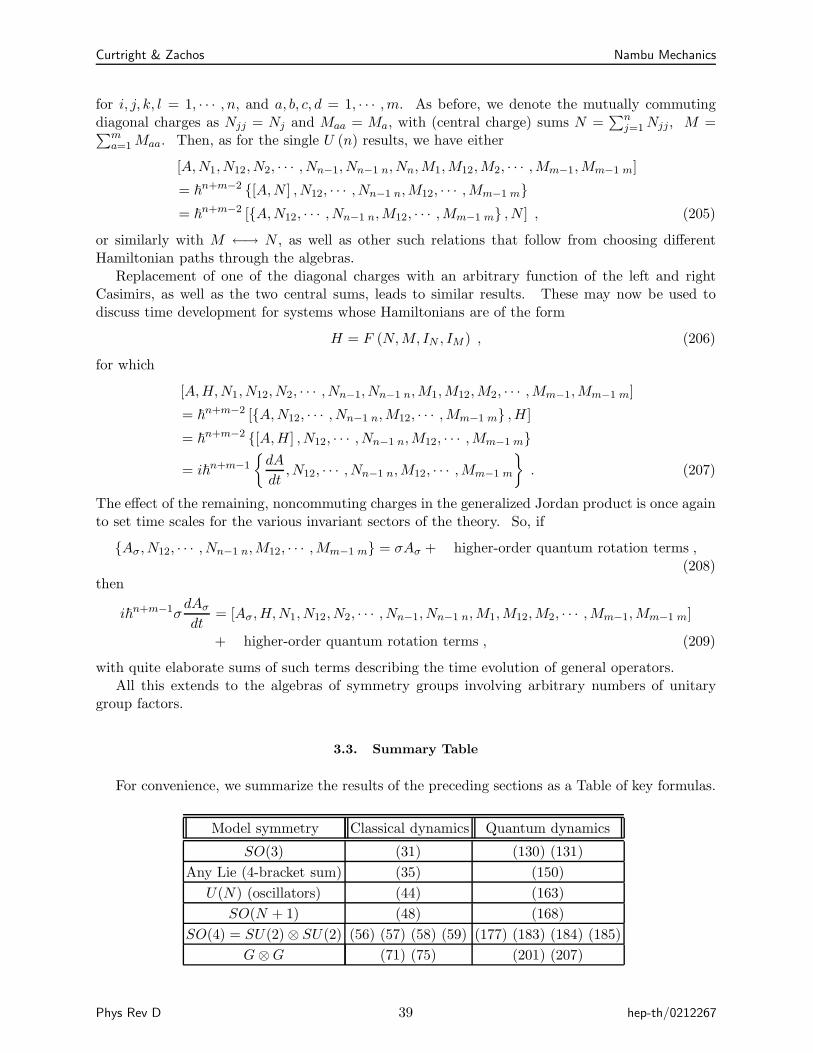
Curtright & Zachos Nambu Mechanics
for i, j, k, l = 1, · · · , n, and a, b, c, d = 1, · · · ,m. As before, we denote the mutually commutingdiagonal charges as Njj = Nj and Maa = Ma, with (central charge) sums N =
∑nj=1 Njj, M =
∑ma=1 Maa. Then, as for the single U (n) results, we have either
[A,N1, N12, N2, · · · , Nn−1, Nn−1 n, Nn,M1,M12,M2, · · · ,Mm−1,Mm−1 m]
= ~n+m−2 [A,N ] , N12, · · · , Nn−1 n,M12, · · · ,Mm−1 m
= ~n+m−2 [A,N12, · · · , Nn−1 n,M12, · · · ,Mm−1 m , N ] , (205)
or similarly with M ←→ N , as well as other such relations that follow from choosing differentHamiltonian paths through the algebras.
Replacement of one of the diagonal charges with an arbitrary function of the left and rightCasimirs, as well as the two central sums, leads to similar results. These may now be used todiscuss time development for systems whose Hamiltonians are of the form
H = F (N,M, IN , IM ) , (206)
for which
[A,H,N1, N12, N2, · · · , Nn−1, Nn−1 n,M1,M12,M2, · · · ,Mm−1,Mm−1 m]
= ~n+m−2 [A,N12, · · · , Nn−1 n,M12, · · · ,Mm−1 m ,H]
= ~n+m−2 [A,H] , N12, · · · , Nn−1 n,M12, · · · ,Mm−1 m
= i~n+m−1
dA
dt,N12, · · · , Nn−1 n,M12, · · · ,Mm−1 m
. (207)
The effect of the remaining, noncommuting charges in the generalized Jordan product is once againto set time scales for the various invariant sectors of the theory. So, if
Aσ, N12, · · · , Nn−1 n,M12, · · · ,Mm−1 m = σAσ + higher-order quantum rotation terms ,(208)
then
i~n+m−1σdAσ
dt= [Aσ,H,N1, N12, N2, · · · , Nn−1, Nn−1 n,M1,M12,M2, · · · ,Mm−1,Mm−1 m]
+ higher-order quantum rotation terms , (209)
with quite elaborate sums of such terms describing the time evolution of general operators.All this extends to the algebras of symmetry groups involving arbitrary numbers of unitary
group factors.
3.3. Summary Table
For convenience, we summarize the results of the preceding sections as a Table of key formulas.
Model symmetry Classical dynamics Quantum dynamics
SO(3) (31) (130) (131)
Any Lie (4-bracket sum) (35) (150)
U(N) (oscillators) (44) (163)
SO(N + 1) (48) (168)
SO(4) = SU(2)⊗ SU(2) (56) (57) (58) (59) (177) (183) (184) (185)
G⊗G (71) (75) (201) (207)
Phys Rev D 39 hep-th/0212267
Curtright & Zachos Nambu Mechanics
An empirical methodology suggested by the above examples argues for the following checklistin quantizing a general classical system of the type (24). If V is trivial (i.e. numerical), theQNB corresponding to the CNB involved is a prime candidate for an “exceptional” derivationquantization, provided the derivation property checks (and thus the EFI). In the generic case, ifV is a function of the invariants, manipulation of the classical expression may be useful, to resultin a simpler V , and in new CNB entries which would still combine into the Hamiltonian in the PBresolution. The corresponding QNB would then be expected to yield the entwined structures to bestudied as above, with the Hamiltonian appearing as an entwined commutator (time derivative),and with the respective time scale eigenvalue problems to be solved.
4. CONCLUSIONS
In this paper, we have demonstrated and illustrated through simple, explicit examples, howNambu brackets provide a consistent, elegant description, both classically and quantum mechani-cally, especially of superintegrable systems using even QNBs. This description can be equivalent toclassical and quantum Hamiltonian mechanics, but it is broader in its conceptualizations and mayhave more possible uses. In particular, we have explained in detail how QNBs are consistent, afterall, given due consideration to multiple time scales set by invariants entwining the time derivatives,and how reputed inconsistencies have instead involved unsuitable and untenable conditions. Wehave also emphasized additional complications that distinguish odd QNBs.
We believe the physical interpretations of entwined time derivatives, with their dynamical timescales, and group rotations, in the general situation, explain the perceived failure of the classicalLeibniz rules and the classical FI in a transparent way, and are the only ingredients requiredfor a successful non-Abelian quantum implementation of the most general Nambu brackets asdescriptions of dynamics. Perhaps this approach is equivalent to the Abelian deformation approach[18], but that has not been shown. However, ultimately it should not be necessary to have toargue, physically, that if the Abelian deformation approach to quantization of Nambu brackets isindeed logically complete and consistent, then it must give specific results equivalent to the moretraditional noncommutative operator approach given here. There is, after all, not very muchfreedom in the quantization of free particles and simple harmonic oscillators!
Moreover, Hanlon and Wachs [24] announced the result that even QNB algebras (designatedby them as “Lie k-algebras”) are “Koszul” (also see [4]), and therefore have duals which arecommutative and totally associative. Is it possible that the Abelian deformation quantizationof Nambu brackets is precisely this dual, and is in that sense equivalent mathematically to thenon-Abelian structures we have discussed?
Other such mathematical issues and areas for further study are raised by our analysis, such as:A complete mathematical classification of Jordan-Kurosh eigenvalue problems; a correspondingtreatment of quantum rotation terms; a study of both classical and quantum topological effectsin terms of Nambu brackets; and the behavior of the brackets in the large N limit (as one way toobtain a field theory).
There are also several open avenues for physical applications, the most promising involvingmembranes and other extended objects. In that regard, given the quantum dichotomy of evenand odd brackets, it would appear that extended objects with alternate-dimensional world-volumesare more amenable to QNBs. While volume preserving diffeomorphisms are based on classicalgeometrical concepts, perhaps relying too strongly on associativity, their ultimate generalizationto noncommutative geometries, and their uses in field, string, and membrane theories, shouldbe possible. We hope the developments in this paper contribute towards completion of suchenterprises.
Phys Rev D 40 hep-th/0212267
Curtright & Zachos Nambu Mechanics
Acknowledgments
We thank Y Nambu and Y Nutku for helpful discussions, and J de Azcarraga for pointing outrelated earlier work, as well as a critical reading of the manuscript. We also thank D Fairliefor informative remarks, in particular for reminding us of Laplace’s theorem on general minorexpansions. This research was supported in part by the US Department of Energy, Division ofHigh Energy Physics, Contract W-31-109-ENG-38, and in part by NSF Award 0073390.
APPENDIX A: FORMAL DIVISION
We are often interested in solving non-linear algebraic equations in both Lie and special Jordanalgebras. This is hampered by the fact that these are not division rings.
Nevertheless, there is a formal series solution to construct inverses in both special Jordan andLie algebras as contained in an associative embedding algebra A. For the former, consider17
a b = b a ≡ ab + ba = c . (A1)
Suppose b and c are given. We wish to solve for a. We assume the inverse b−1 exists in theenveloping algebra. So we seek to construct either right b−1
R or left b−1L inverses under Jordan
multiplication , so that a = c b−1R = b−1
L c. A formal series solution for b−1R is obtained from
the inverse b−1 in the enveloping algebra by writing a = cb−1 − bab−1, and iterating. Thus,
a = cb−1 − bcb−2 + b2ab−2 =
(
∞∑
n=0
(−1)n bncb−n
)
b−1 ≡ c b−1R . (A2)
Similarly, for the left inverse a = b−1c− b−1ab, so
a = b−1c− b−2cb + b−2ab2 = b−1
(
∞∑
n=0
(−1)n b−ncbn
)
≡ b−1L c . (A3)
Requiring formally that these two inverses give the same a leads to an expression that involvesonly Jordan products of elements from the enveloping algebra,
a =1
2
∞∑
n=0
(−1)n(
bncb−n−1 + b−n−1cbn)
=1
2
∞∑
n=0
(−1)n (bncbn) b−2n−1 . (A4)
However, it involves an infinite number of such products. This raises convergence issues, evenwhen b−1 exists in the enveloping algebra.
As the simplest possible illustration of the convergence issues, suppose b and c commute, bc =cb. Then either of the above series for left or right inverses gives an ill-defined result, a =b−1c
∑∞n=0 (−1)n. Evidently, the proper way to interpret the (Borel summable) series in this case
is∑∞
n=0 (−1)n = 11−(−1) = 1
2 , to produce the solution to the original equation when ab = ba as well
as bc = cb. Namely, 2ab = c and a = 12b−1c. Nevertheless, convergence is a problem.
For the Lie case, the same formal approach may be considered. Let
a ⋄ b = −b ⋄ a ≡ ab− ba = c . (A5)
17 Jordan would include a factor of 1/2 in the definition of .
Phys Rev D 41 hep-th/0212267
Curtright & Zachos Nambu Mechanics
Suppose b and c are given and solve for a. That is, construct either right b−1R or left b−1
L inversesunder Lie multiplication, ⋄, so that a = c ⋄ b−1
R = −b−1L ⋄ c. Again, these are given by formal series
solutions obtained by writing a = cb−1 + bab−1 and iterating. Thus,
a = cb−1 + bcb−2 + b2ab−2 =
(
∞∑
n=0
bncb−n
)
b−1 ≡ c ⋄ b−1R . (A6)
Similarly, for the left inverse a = −b−1c + b−1ab, so
a = −b−1c− b−2cb + b−2ab2 = −b−1
(
∞∑
n=0
b−ncbn
)
≡ −b−1L ⋄ c . (A7)
Requiring that these two inverses give the same a leads to an expression that involves only Lieproducts of elements from the enveloping algebra,
a =1
2
∞∑
n=0
(
bncb−n−1 − b−n−1cbn)
≡ 1
2
∞∑
n=0
(bncbn) ⋄ b−2n−1 . (A8)
But, once more, it involves an infinite number of such products. Again this raises convergenceissues, even when b−1 exists in the enveloping algebra.
As an illustration of convergence issues in this case, follow Wigner’s counsel and take 2 × 2matrices, b = σy = b−1 and c = 2iσz. Then, for even n, (bncbn) ⋄ b−2n−1 = [c, b] = 4σx; whilefor odd n, (bncbn) ⋄ b−2n−1 = [bcb, b] = − [c, b] = −4σx. Again, the series gives an ill-definedresult, a = 1
2 4σx
∑∞n=0 (−1)n. This shows clearly that convergence is again a problem. As
before, the proper way to interpret the sum in this particular example is∑∞
n=0 (−1)n = 12 , to
produce the obvious solution to the original equation, a = σx.The failed convergence for these series is accompanied by a basic problem: divisors of zero.
Even when b is invertible in the enveloping algebra, so that the only solution of ab = 0 is a = 0,this does not hold for the Jordan or Lie products. The Lie case is most familiar and easily seen.a ⋄ b = 0 always has an infinite number of nonvanishing solutions a 6= 0. Namely, a = κb forany parameter κ 6= 0. Moreover, there can and will be other independent solutions for higherdimensional enveloping algebras. That is to say, Lie algebras are not division rings, even whenthey only involve commutators of invertible elements from A. The same is true for the Jordancase, in general. For instance, using the 2× 2 matrices as an example, again with b = σy, we havea b = 0 for a = κσz + λσx for any parameters κ and λ. So, as stressed already, special Jordanalgebras are not division rings – not even when they involve only anticommutators of invertibleelements from A.
Perhaps one way to avoid these difficulties and place the formal series constructions on a firmerfooting would be through regularizing deformations of the algebras. This works for the specificJordan or Lie examples above, as illustrations of the method. Rather than the Jordan or Lieproducts, take ab + λba = c. (This deformation was actually analyzed in Jordan’s original paper[29], before he settled on the λ = 1 case.) This yields a convergent series for the right inverse b−1
R
when |λ| < 1, and a convergent series for the left inverse b−1L when |λ| > 1. For the right inverse,
write a = cb−1 − λbab−1, and iterate. Thus
a = cb−1 − λbcb−2 + λ2b2ab−2 =
(
∞∑
n=0
(−λ)n bncb−n
)
b−1 . (A9)
For the simplest situation where bc = cb, this gives
a = b−1c
(
∞∑
n=0
(−λ)n)
= b−1c1
1 + λ. (A10)
Phys Rev D 42 hep-th/0212267
Curtright & Zachos Nambu Mechanics
Now the correct result emerges in the limit λ → 1, but strictly speaking this is not within theradius of convergence of the series. The series must first be summed to obtain a meromorphicfunction, by analytic continuation, and the limit applied to that function.
The same method works for the simple Lie example given above. Again, suppose b = σy = b−1
and let c = 2iσz . The series for the right inverse now gives a = 12 4σx
∑∞n=0 λn = 2
1−λσx. The
limit λ → −1 converts both this solution and the original equation ab + λba = c into the Lieproblem of interest a ⋄ b = c.
[1] A C Aitken, Determinants and Matrices, Greenwood Publishing Group, 1983 (reprint).[2] H Awata, M Li, D Minic, and T Yoneya, “On the Quantization of Nambu Brackets” JHEP 02 (2001)
013 [hep-th/9906248].[3] S Ayupov, A Rakhimov, and S Usmanov, Jordan, real, and Lie structures in operator algebras, Kluwer
Academic Publishers, Boston, 1997.[4] J A de Azcarraga, A. M. Perelomov, and J C Perez Bueno, “The Schouten-Nijenhuis bracket, coho-
mology and generalized Poisson structures” J Phys A29 (1996) 7993-8010 [hep-th/9605067].[5] J A de Azcarraga, and J C Perez Bueno, “Higher-order simple Lie algebras” Commun Math Phys 184
(1997) 669-681 [hep-th/9605213].[6] J A de Azcarraga, J M Izquierdo, and J C Perez Bueno, “On the generalizations of Poisson structures”
J Phys A30 (1997) L607-L616 [hep-th/9703019] ; “An introduction to some novel applications of Liealgebra cohomology in mathematics and physics” Rev R Acad Cien Serie A Mat 95 (2001) 225-248[physics/9803046].
[7] L Baker and D B Fairlie, “Hamilton-Jacobi equations and Brane associated Lagrangians” Nucl PhysB596 (2001) 348-364 [hep-th/0003048].
[8] M Baranovich and M S Burgin, “Linear Ω-Algebras” Russian Math Surveys 30 (1975) 65-113.[9] F Bayen and M Flato, “Remarks concerning Nambu’s generalized mechanics” Phys Rev D11 (1975)
3049-3053.[10] E Braaten, T Curtright, and C Zachos, “Torsion and Geometrostasis in Nonlinear Sigma Models” Nucl
Phys B260 (1985) 630-688.[11] F Calogero, “Partially Superintegrable Systems and Nonlinear Harmonic Oscillators” talk at the Work-
shop on Superintegrability in Classical and Quantum Systems, Centre de recherches mathematiques,Universite de Montreal, 16 - 21 September 2002.
[12] R Chatterjee, “Dynamical Symmetries and Nambu Mechanics” Lett Math Phys 36 (1996) 117-126[hep-th/9501141].
[13] T Curtright, “Schrodinger’s Cataplex” pp 121-131 Quantum gravity, generalized theory of gravitation,and superstring theory-based unification, B Kursunoglu, S Mintz, and A Perlmutter (editors), KluwerAcademic, New York 2000 (28th Orbis Scientiae Conference, 1999) [quant-ph/0011101].
[14] T Curtright and D Fairlie, “Extra Dimensions and Nonlinear Equations” to appear in J Math Phys[math-ph/0207008].
[15] T Curtright, T Uematsu, and C Zachos, “Geometry and duality in supersymmetric σ-models” NuclPhys B469 (1996) 488-512 [hep-th/0011137].
[16] T L Curtright and C K Zachos, “Deformation Quantization of Superintegrable Systems and NambuMechanics” N J Phys 4 (2002) 83 [hep-th/0205063]; “Nambu Dynamics, Deformation Quantization, andSuperintegrability” talk at the Workshop on Superintegrability in Classical and Quantum Systems, Cen-tre de recherches mathematiques, Universite de Montreal, 16 - 21 September 2002 [math-ph/0211021];“Quantizing Dirac and Nambu Brackets” talk at the Coral Gables Conference, 11-14 December 2002[hep-th/0303088].
[17] G Dito and M Flato, “Generalized Abelian Deformations: Application to Nambu Mechanics” LettMath Phys 39 (1997) 107-125 [hep-th/9609114].
[18] G Dito, M Flato, D Sternheimer, and L Takhtajan, “Deformation Quantization and Nambu Mechanics”Comm Math Phys 183 (1997) 1-22 [hep-th/9602016].
[19] F B Estabrook, “Comments on Generalized Hamiltonian Dynamics” Phys Rev D8 (1973) 2740-2743.
Phys Rev D 43 hep-th/0212267
Curtright & Zachos Nambu Mechanics
[20] V T Filippov, “n-Lie Algebras” Sib Mat Zh 26 (1985) 126-140 (English translation: Sib Math Journal26 (1986) 879-891).
[21] J-P Francoise, “Perturbation theory of superintegrable systems” talk at the Workshop on Superintegra-bility in Classical and Quantum Systems, Centre de recherches mathematiques, Universite de Montreal,16 - 21 September 2002.
[22] P Gautheron, “Some Remarks Concerning Nambu Mechanics” Lett Math Phys 37 (1996) 103-116.[23] C Gonera and Y Nutku, “Super-integrable Calogero-type systems admit maximal number of Poisson
structures” Phys Lett A285 (2001) 301-306.[24] P Hanlon and M Wachs, “On Lie k-Algebras” Adv Math 113 (1995) 206-236.[25] J Hietarinta, “Nambu tensors and commuting vector fields” J Phys A30 (1997) L27-L33.[26] P Higgins, “Groups with multiple operators” Proc London Math Soc 6 (1956) 366–416.[27] J Hoppe, “On M Algebras, the Quantization of Nambu Mechanics, and Volume Preserving Diffeomor-
phisms” Helv Phys Acta 70 (1997) 302-317 [hep-th/9602020].[28] N Jacobson, “Lie and Jordan triple systems” Am J Math 71 (1949) 149-170;
“General representation theory of Jordan algebras” Trans Am Math Soc 70 (1950) 509–530.[29] P Jordan, “Uber die Multiplikation quantenmechanischer Großen” Z Phys 80 (1933) 285-291;
P Jordan, J von Neumann, and E Wigner, “On an algebraic generalization of the quantum mechanicalformalism” Ann Math 35 (1934) 29-64.
[30] A J Kalnay and R Tascon, “On Lagrange, Hamilton-Dirac, and Nambu mechanics” Phys Rev D17
(1978) 1552-1562.[31] R Kerner, “Ternary Algebraic Structures and their Applications in Physics” [math-ph/0011023].[32] A G Kurosh, “Multioperator Rings and Algebras” Russian Math Surveys 24 (1969) 1-13.[33] W Lister, “A structure theory of Lie triple systems” Trans Am Math Soc 72 (1952) 217–242.[34] Y Matsuo and Y Shibusa, “Volume preserving diffeomorphism and noncommutative branes” JHEP 02
(2001) 006 [hep-th/0010040].[35] D Minic, “M Theory and Deformation Quantization” [hep-th/9909022].[36] D Minic and C-H Tze, “Nambu Quantum Mechanics: A Nonlinear Generalization of Geometric Quan-
tum Mechanics” Phys Lett B536 (2002) 305-314 [hep-th/0202173].[37] N Mukunda and E Sudarshan, “Relation between Nambu and Hamiltonian mechanics” Phys Rev D13
(1976) 2846-2850.[38] Y Nambu, “Generalized Hamiltonian Dynamics” Phys Rev D7 (1973) 2405-2412.[39] Y Nutku, “Quantization of superintegrable systems with Nambu-Poisson brackets” talk at the Work-
shop on Superintegrability in Classical and Quantum Systems, Centre de recherches mathematiques,Universite de Montreal, 16 - 21 September 2002; “Quantization with Nambu-Poisson brackets: Theharmonic oscillator!” J Phys A, in press.
[40] B Pioline, “Comments on the Topological Open Membrane” Phys Rev D66 (2002) 025010[hep-th/0201257].
[41] D Sahoo and M C Valsakumar, “Nambu mechanics and its quantization” Phys Rev A46 (1992) 4410-4412; “Nonexistence of Nambu Quantum Mechanics” Mod Phys Lett A9 (1994) 2727-2732.
[42] M Sakakibara, “Remarks on a Deformation Quantization of the Canonical Nambu Bracket” Prog TheorPhys 104 (2000) 1067-1071.
[43] M Schlesinger and J D Stasheff, “The Lie algebra structure of tangent cohomology and deformationtheory” J Pure Appl Algebra 38 (1985) 313-322.
[44] L Takhtajan, “On foundation of the generalized Nambu mechanics” Comm Math Phys 160 (1994)295–315 [hep-th/9301111].
[45] P Tempesta, A V Turbiner, and P Winternitz, “Exact solvability of superintegrable systems” J MathPhys 42 (2001) 4248-4257 [hep-th/0011209].
[46] L Vainerman and R Kerner, “On special classes of n-algebras” J Math Physics 37 (1996) 2553-2565.[47] Chuan-sheng Xiong, “Remark on Quantum Nambu Bracket” Phys Lett B486 (2000) 228-231
[hep-th/0003292].[48] C K Zachos and T L Curtright, “Deformation Quantization, Superintegrability, and Nambu Mechan-
ics” [hep-th/0210170]; “Deformation Quantization of Nambu Mechanics” talk at the Coral GablesConference, 11-14 December 2002 [quant-ph/0302106].
Phys Rev D 44 hep-th/0212267
Related Documents


![[Kibble] - Classical Mechanics](https://static.cupdf.com/doc/110x72/552056344a79596f718b4715/kibble-classical-mechanics.jpg)