Christopher Dougherty EC220 - Introduction to econometrics (chapter 1) Slideshow: exercise 1.16 Original citation: Dougherty, C. (2012) EC220 - Introduction.

Christopher Dougherty

EC220 - Introduction to econometrics (chapter 1)Slideshow: exercise 1.16

Original citation:

Dougherty, C. (2012) EC220 - Introduction to econometrics (chapter 1). [Teaching Resource]

© 2012 The Author

This version available at: http://learningresources.lse.ac.uk/127/

Available in LSE Learning Resources Online: May 2012

This work is licensed under a Creative Commons Attribution-ShareAlike 3.0 License. This license allows the user to remix, tweak, and build upon the work even for commercial purposes, as long as the user credits the author and licenses their new creations under the identical terms. http://creativecommons.org/licenses/by-sa/3.0/

 http://learningresources.lse.ac.uk/

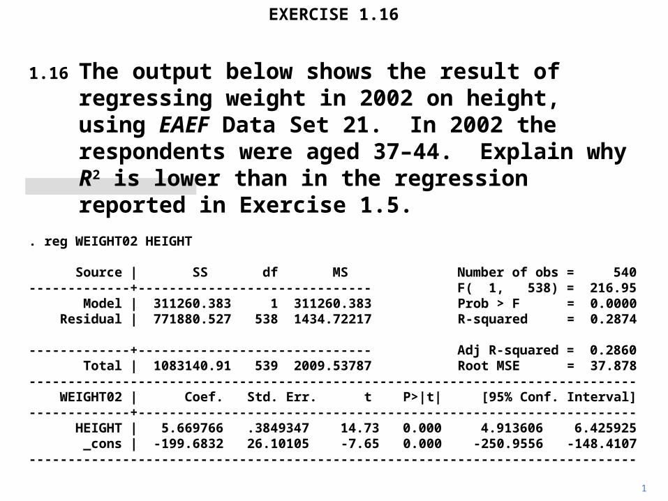
1.16 The output below shows the result of regressing weight in 2002 on height, using EAEF Data Set 21. In 2002 the respondents were aged 37–44. Explain why R2 is lower than in the regression reported in Exercise 1.5.

. reg WEIGHT02 HEIGHT

Source | SS df MS Number of obs = 540-------------+------------------------------ F( 1, 538) = 216.95 Model | 311260.383 1 311260.383 Prob > F = 0.0000 Residual | 771880.527 538 1434.72217 R-squared = 0.2874

-------------+------------------------------ Adj R-squared = 0.2860 Total | 1083140.91 539 2009.53787 Root MSE = 37.878------------------------------------------------------------------------------ WEIGHT02 | Coef. Std. Err. t P>|t| [95% Conf. Interval]-------------+---------------------------------------------------------------- HEIGHT | 5.669766 .3849347 14.73 0.000 4.913606 6.425925 _cons | -199.6832 26.10105 -7.65 0.000 -250.9556 -148.4107------------------------------------------------------------------------------

EXERCISE 1.16

1

2

EXERCISE 1.16

The regression output above gives the result of regressing weight, measured in pounds, on height, measured in inches, using EAEF Data Set 21.

. reg WEIGHT85 HEIGHT Source | SS df MS Number of obs = 540-------------+-------------------------- F( 1, 538) = 355.97 Model | 261111.383 1 261111.383 Prob > F = 0.0000Residual | 394632.365 538 733.517407 R-squared = 0.3982-------------+-------------------------- Adj R-squared = 0.3971 Total | 655743.748 539 1216.59322 Root MSE = 27.084------------------------------------------------------------------------------WEIGHT85 | Coef. Std. Err. t P>|t| [95% Conf. Interval]-------------+---------------------------------------------------------------- HEIGHT | 5.192973 .275238 18.87 0.000 4.6523 5.733646 _cons | -194.6815 18.6629 -10.43 0.000 -231.3426 -158.0204------------------------------------------------------------------------------

. reg WEIGHT02 HEIGHT Source | SS df MS Number of obs = 540-------------+-------------------------- F( 1, 538) = 216.95 Model | 311260.383 1 311260.383 Prob > F = 0.0000Residual | 771880.527 538 1434.72217 R-squared = 0.2874-------------+-------------------------- Adj R-squared = 0.2860 Total | 1083140.91 539 2009.53787 Root MSE = 37.878------------------------------------------------------------------------------WEIGHT02 | Coef. Std. Err. t P>|t| [95% Conf. Interval]-------------+---------------------------------------------------------------- HEIGHT | 5.669766 .3849347 14.73 0.000 4.913606 6.425925 _cons | -199.6832 26.10105 -7.65 0.000 -250.9556 -148.4107------------------------------------------------------------------------------

3

EXERCISE 1.16

The first regression uses weight measured in 1985, when the respondents were aged 20 to 27. The second uses weight measured 17 years later in 2002.

. reg WEIGHT85 HEIGHT Source | SS df MS Number of obs = 540-------------+-------------------------- F( 1, 538) = 355.97 Model | 261111.383 1 261111.383 Prob > F = 0.0000Residual | 394632.365 538 733.517407 R-squared = 0.3982-------------+-------------------------- Adj R-squared = 0.3971 Total | 655743.748 539 1216.59322 Root MSE = 27.084------------------------------------------------------------------------------WEIGHT85 | Coef. Std. Err. t P>|t| [95% Conf. Interval]-------------+---------------------------------------------------------------- HEIGHT | 5.192973 .275238 18.87 0.000 4.6523 5.733646 _cons | -194.6815 18.6629 -10.43 0.000 -231.3426 -158.0204------------------------------------------------------------------------------

. reg WEIGHT02 HEIGHT Source | SS df MS Number of obs = 540-------------+-------------------------- F( 1, 538) = 216.95 Model | 311260.383 1 311260.383 Prob > F = 0.0000Residual | 771880.527 538 1434.72217 R-squared = 0.2874-------------+-------------------------- Adj R-squared = 0.2860 Total | 1083140.91 539 2009.53787 Root MSE = 37.878------------------------------------------------------------------------------WEIGHT02 | Coef. Std. Err. t P>|t| [95% Conf. Interval]-------------+---------------------------------------------------------------- HEIGHT | 5.669766 .3849347 14.73 0.000 4.913606 6.425925 _cons | -199.6832 26.10105 -7.65 0.000 -250.9556 -148.4107------------------------------------------------------------------------------

. reg WEIGHT85 HEIGHT Source | SS df MS Number of obs = 540-------------+-------------------------- F( 1, 538) = 355.97 Model | 261111.383 1 261111.383 Prob > F = 0.0000Residual | 394632.365 538 733.517407 R-squared = 0.3982-------------+-------------------------- Adj R-squared = 0.3971 Total | 655743.748 539 1216.59322 Root MSE = 27.084------------------------------------------------------------------------------WEIGHT85 | Coef. Std. Err. t P>|t| [95% Conf. Interval]-------------+---------------------------------------------------------------- HEIGHT | 5.192973 .275238 18.87 0.000 4.6523 5.733646 _cons | -194.6815 18.6629 -10.43 0.000 -231.3426 -158.0204------------------------------------------------------------------------------

. reg WEIGHT02 HEIGHT Source | SS df MS Number of obs = 540-------------+-------------------------- F( 1, 538) = 216.95 Model | 311260.383 1 311260.383 Prob > F = 0.0000Residual | 771880.527 538 1434.72217 R-squared = 0.2874-------------+-------------------------- Adj R-squared = 0.2860 Total | 1083140.91 539 2009.53787 Root MSE = 37.878------------------------------------------------------------------------------WEIGHT02 | Coef. Std. Err. t P>|t| [95% Conf. Interval]-------------+---------------------------------------------------------------- HEIGHT | 5.669766 .3849347 14.73 0.000 4.913606 6.425925 _cons | -199.6832 26.10105 -7.65 0.000 -250.9556 -148.4107------------------------------------------------------------------------------

4

EXERCISE 1.16

The explained sum of squares (called by Stata the model sum of squares) is actually higher for 2002 than for 1985. So why is R2 considerably lower in the second regression? (The next slide gives the answer, so think about it first.)

5

EXERCISE 1.16

As people age, they tend to put on weight. For this sample, mean weight was 157 pounds in 1985, and 184 pounds in 2002.

. reg WEIGHT85 HEIGHT Source | SS df MS Number of obs = 540-------------+-------------------------- F( 1, 538) = 355.97 Model | 261111.383 1 261111.383 Prob > F = 0.0000Residual | 394632.365 538 733.517407 R-squared = 0.3982-------------+-------------------------- Adj R-squared = 0.3971 Total | 655743.748 539 1216.59322 Root MSE = 27.084------------------------------------------------------------------------------WEIGHT85 | Coef. Std. Err. t P>|t| [95% Conf. Interval]-------------+---------------------------------------------------------------- HEIGHT | 5.192973 .275238 18.87 0.000 4.6523 5.733646 _cons | -194.6815 18.6629 -10.43 0.000 -231.3426 -158.0204------------------------------------------------------------------------------

. reg WEIGHT02 HEIGHT Source | SS df MS Number of obs = 540-------------+-------------------------- F( 1, 538) = 216.95 Model | 311260.383 1 311260.383 Prob > F = 0.0000Residual | 771880.527 538 1434.72217 R-squared = 0.2874-------------+-------------------------- Adj R-squared = 0.2860 Total | 1083140.91 539 2009.53787 Root MSE = 37.878------------------------------------------------------------------------------WEIGHT02 | Coef. Std. Err. t P>|t| [95% Conf. Interval]-------------+---------------------------------------------------------------- HEIGHT | 5.669766 .3849347 14.73 0.000 4.913606 6.425925 _cons | -199.6832 26.10105 -7.65 0.000 -250.9556 -148.4107------------------------------------------------------------------------------

6

EXERCISE 1.16

Some people are more successful in resisting this tendency than others, either because of their genetic make-up or because they have a healthier life-style.

. reg WEIGHT85 HEIGHT Source | SS df MS Number of obs = 540-------------+-------------------------- F( 1, 538) = 355.97 Model | 261111.383 1 261111.383 Prob > F = 0.0000Residual | 394632.365 538 733.517407 R-squared = 0.3982-------------+-------------------------- Adj R-squared = 0.3971 Total | 655743.748 539 1216.59322 Root MSE = 27.084------------------------------------------------------------------------------WEIGHT85 | Coef. Std. Err. t P>|t| [95% Conf. Interval]-------------+---------------------------------------------------------------- HEIGHT | 5.192973 .275238 18.87 0.000 4.6523 5.733646 _cons | -194.6815 18.6629 -10.43 0.000 -231.3426 -158.0204------------------------------------------------------------------------------

. reg WEIGHT02 HEIGHT Source | SS df MS Number of obs = 540-------------+-------------------------- F( 1, 538) = 216.95 Model | 311260.383 1 311260.383 Prob > F = 0.0000Residual | 771880.527 538 1434.72217 R-squared = 0.2874-------------+-------------------------- Adj R-squared = 0.2860 Total | 1083140.91 539 2009.53787 Root MSE = 37.878------------------------------------------------------------------------------WEIGHT02 | Coef. Std. Err. t P>|t| [95% Conf. Interval]-------------+---------------------------------------------------------------- HEIGHT | 5.669766 .3849347 14.73 0.000 4.913606 6.425925 _cons | -199.6832 26.10105 -7.65 0.000 -250.9556 -148.4107------------------------------------------------------------------------------

7

EXERCISE 1.16

Thus the variance in weight also tends to increase. You can see that there has been a huge increase in the total sum of squares.

. reg WEIGHT85 HEIGHT Source | SS df MS Number of obs = 540-------------+-------------------------- F( 1, 538) = 355.97 Model | 261111.383 1 261111.383 Prob > F = 0.0000Residual | 394632.365 538 733.517407 R-squared = 0.3982-------------+-------------------------- Adj R-squared = 0.3971 Total | 655743.748 539 1216.59322 Root MSE = 27.084------------------------------------------------------------------------------WEIGHT85 | Coef. Std. Err. t P>|t| [95% Conf. Interval]-------------+---------------------------------------------------------------- HEIGHT | 5.192973 .275238 18.87 0.000 4.6523 5.733646 _cons | -194.6815 18.6629 -10.43 0.000 -231.3426 -158.0204------------------------------------------------------------------------------

. reg WEIGHT02 HEIGHT Source | SS df MS Number of obs = 540-------------+-------------------------- F( 1, 538) = 216.95 Model | 311260.383 1 311260.383 Prob > F = 0.0000Residual | 771880.527 538 1434.72217 R-squared = 0.2874-------------+-------------------------- Adj R-squared = 0.2860 Total | 1083140.91 539 2009.53787 Root MSE = 37.878------------------------------------------------------------------------------WEIGHT02 | Coef. Std. Err. t P>|t| [95% Conf. Interval]-------------+---------------------------------------------------------------- HEIGHT | 5.669766 .3849347 14.73 0.000 4.913606 6.425925 _cons | -199.6832 26.10105 -7.65 0.000 -250.9556 -148.4107------------------------------------------------------------------------------

8

EXERCISE 1.16

Consequently, although the explained sum of squares accounted for by height has increased, it has become a smaller proportion of the total sum of squares and R2 has fallen.

. reg WEIGHT85 HEIGHT Source | SS df MS Number of obs = 540-------------+-------------------------- F( 1, 538) = 355.97 Model | 261111.383 1 261111.383 Prob > F = 0.0000Residual | 394632.365 538 733.517407 R-squared = 0.3982-------------+-------------------------- Adj R-squared = 0.3971 Total | 655743.748 539 1216.59322 Root MSE = 27.084------------------------------------------------------------------------------WEIGHT85 | Coef. Std. Err. t P>|t| [95% Conf. Interval]-------------+---------------------------------------------------------------- HEIGHT | 5.192973 .275238 18.87 0.000 4.6523 5.733646 _cons | -194.6815 18.6629 -10.43 0.000 -231.3426 -158.0204------------------------------------------------------------------------------

. reg WEIGHT02 HEIGHT Source | SS df MS Number of obs = 540-------------+-------------------------- F( 1, 538) = 216.95 Model | 311260.383 1 311260.383 Prob > F = 0.0000Residual | 771880.527 538 1434.72217 R-squared = 0.2874-------------+-------------------------- Adj R-squared = 0.2860 Total | 1083140.91 539 2009.53787 Root MSE = 37.878------------------------------------------------------------------------------WEIGHT02 | Coef. Std. Err. t P>|t| [95% Conf. Interval]-------------+---------------------------------------------------------------- HEIGHT | 5.669766 .3849347 14.73 0.000 4.913606 6.425925 _cons | -199.6832 26.10105 -7.65 0.000 -250.9556 -148.4107------------------------------------------------------------------------------

Copyright Christopher Dougherty 1999–2006. This slideshow may be freely copied for personal use.

18.06.06