Christopher Dougherty EC220 - Introduction to econometrics (chapter 10) Slideshow: introduction to maximum likelihood estimation Original citation: Dougherty, C. (2012) EC220 - Introduction to econometrics (chapter 10). [Teaching Resource] © 2012 The Author This version available at: http:// learningresources.lse.ac.uk/136/ Available in LSE Learning Resources Online: May 2012 This work is licensed under a Creative Commons Attribution-ShareAlike 3.0 License. This license allows the user to remix, tweak, and build upon the work even for commercial purposes, as long as the user credits the author and licenses their new creations under the identical terms. http://creativecommons.org/licenses/by-sa/3.0/ http://learningresources.lse.ac.uk/

Welcome message from author
This document is posted to help you gain knowledge. Please leave a comment to let me know what you think about it! Share it to your friends and learn new things together.
Transcript
Christopher Dougherty
EC220 - Introduction to econometrics (chapter 10)Slideshow: introduction to maximum likelihood estimation
Original citation:
Dougherty, C. (2012) EC220 - Introduction to econometrics (chapter 10). [Teaching Resource]
© 2012 The Author
This version available at: http://learningresources.lse.ac.uk/136/
Available in LSE Learning Resources Online: May 2012
This work is licensed under a Creative Commons Attribution-ShareAlike 3.0 License. This license allows the user to remix, tweak, and build upon the work even for commercial purposes, as long as the user credits the author and licenses their new creations under the identical terms. http://creativecommons.org/licenses/by-sa/3.0/
http://learningresources.lse.ac.uk/
1
INTRODUCTION TO MAXIMUM LIKELIHOOD ESTIMATION
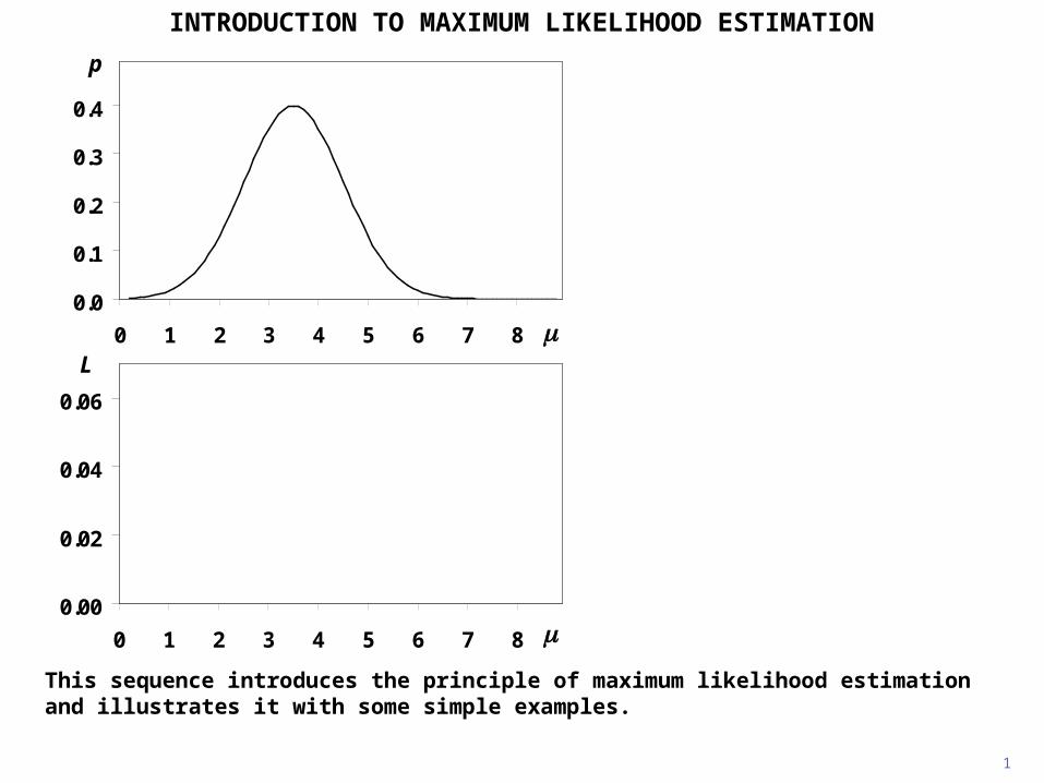
This sequence introduces the principle of maximum likelihood estimation and illustrates it with some simple examples.
L
p
0.0
0.1
0.2
0.3
0.4
0 1 2 3 4 5 6 7 8
0.00
0.02
0.04
0.06
0 1 2 3 4 5 6 7 8
2
INTRODUCTION TO MAXIMUM LIKELIHOOD ESTIMATION
Suppose that you have a normally-distributed random variable X with unknown population mean and standard deviation , and that you have a sample of two observations, 4 and 6. For the time being, we will assume that is equal to 1.
L
p
0.0
0.1
0.2
0.3
0.4
0 1 2 3 4 5 6 7 8
0.00
0.02
0.04
0.06
0 1 2 3 4 5 6 7 8
3
INTRODUCTION TO MAXIMUM LIKELIHOOD ESTIMATION
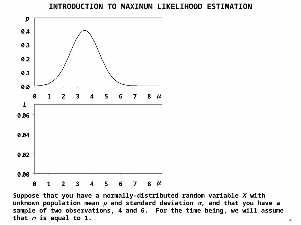
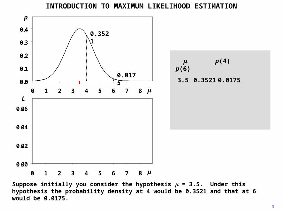
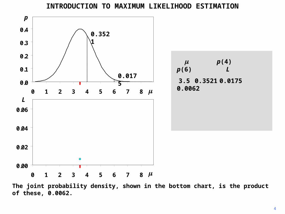
Suppose initially you consider the hypothesis = 3.5. Under this hypothesis the probability density at 4 would be 0.3521 and that at 6 would be 0.0175.
L
p
0.0
0.1
0.2
0.3
0.4
0 1 2 3 4 5 6 7 8
0.00
0.02
0.04
0.06
0 1 2 3 4 5 6 7 8
p(4) p(6)
3.5 0.3521 0.0175
0.3521
0.0175
4
INTRODUCTION TO MAXIMUM LIKELIHOOD ESTIMATION
The joint probability density, shown in the bottom chart, is the product of these, 0.0062.
p(4) p(6) L
3.5 0.3521 0.0175 0.0062
L
p
0.0
0.1
0.2
0.3
0.4
0 1 2 3 4 5 6 7 8
0.00
0.02
0.04
0.06
0 1 2 3 4 5 6 7 8
0.3521
0.0175
5
INTRODUCTION TO MAXIMUM LIKELIHOOD ESTIMATION
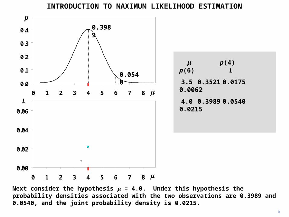
Next consider the hypothesis = 4.0. Under this hypothesis the probability densities associated with the two observations are 0.3989 and 0.0540, and the joint probability density is 0.0215.
p(4) p(6) L
3.5 0.3521 0.0175 0.0062
4.0 0.3989 0.0540 0.0215
L
p
0.00
0.02
0.04
0.06
0 1 2 3 4 5 6 7 8
0.0
0.1
0.2
0.3
0.4
0 1 2 3 4 5 6 7 8
0.3989
0.0540
6
INTRODUCTION TO MAXIMUM LIKELIHOOD ESTIMATION
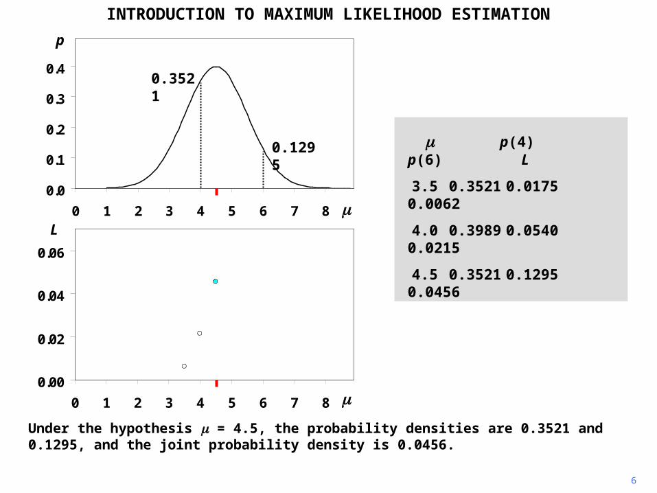
Under the hypothesis = 4.5, the probability densities are 0.3521 and 0.1295, and the joint probability density is 0.0456.
p(4) p(6) L
3.5 0.3521 0.0175 0.0062
4.0 0.3989 0.0540 0.0215
4.5 0.3521 0.1295 0.0456L
p
0.00
0.02
0.04
0.06
0 1 2 3 4 5 6 7 8
0.0
0.1
0.2
0.3
0.4
0 1 2 3 4 5 6 7 8
0.3521
0.1295
7
INTRODUCTION TO MAXIMUM LIKELIHOOD ESTIMATION
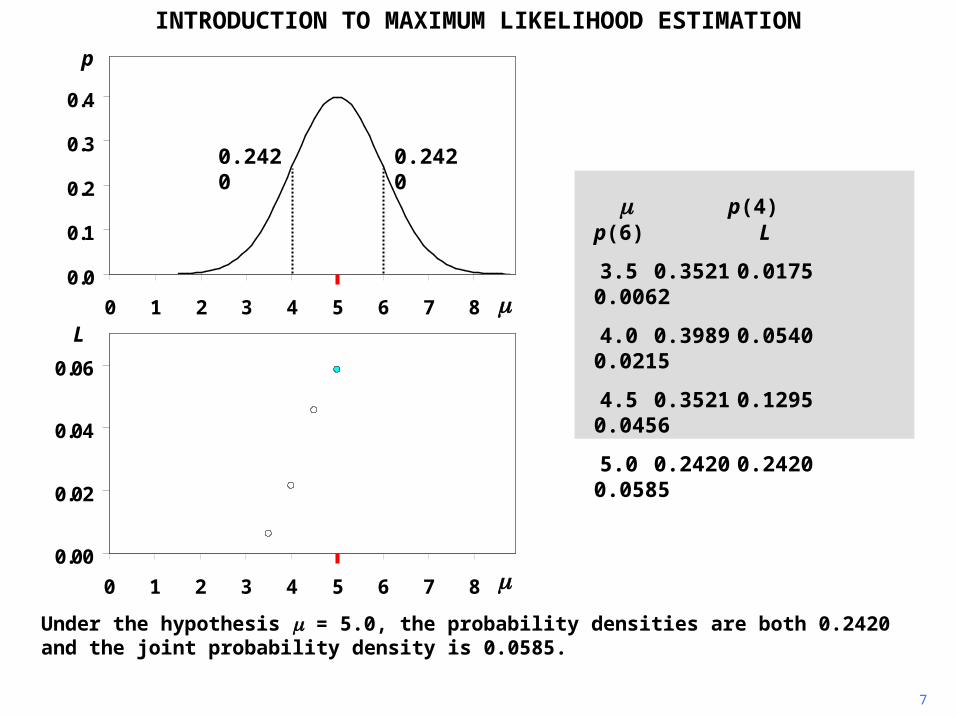
Under the hypothesis = 5.0, the probability densities are both 0.2420 and the joint probability density is 0.0585.
p(4) p(6) L
3.5 0.3521 0.0175 0.0062
4.0 0.3989 0.0540 0.0215
4.5 0.3521 0.1295 0.0456
5.0 0.2420 0.2420 0.0585L
p
0.00
0.02
0.04
0.06
0 1 2 3 4 5 6 7 8
0.0
0.1
0.2
0.3
0.4
0 1 2 3 4 5 6 7 8
0.24200.2420
8
INTRODUCTION TO MAXIMUM LIKELIHOOD ESTIMATION
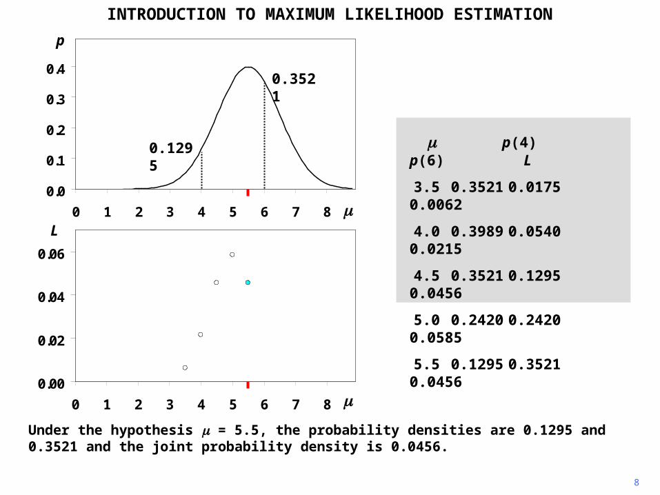
Under the hypothesis = 5.5, the probability densities are 0.1295 and 0.3521 and the joint probability density is 0.0456.
p(4) p(6) L
3.5 0.3521 0.0175 0.0062
4.0 0.3989 0.0540 0.0215
4.5 0.3521 0.1295 0.0456
5.0 0.2420 0.2420 0.0585
5.5 0.1295 0.3521 0.0456
0.0
0.1
0.2
0.3
0.4
0 1 2 3 4 5 6 7 8
0.00
0.02
0.04
0.06
0 1 2 3 4 5 6 7 8
L
p
0.3521
0.1295
9
INTRODUCTION TO MAXIMUM LIKELIHOOD ESTIMATION
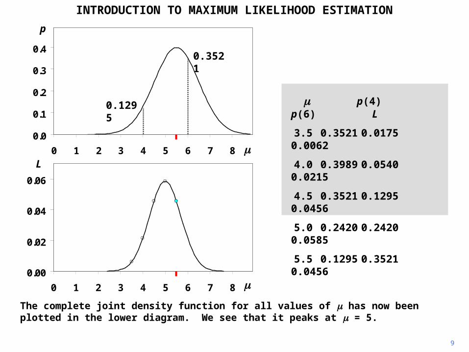
The complete joint density function for all values of has now been plotted in the lower diagram. We see that it peaks at = 5.
p(4) p(6) L
3.5 0.3521 0.0175 0.0062
4.0 0.3989 0.0540 0.0215
4.5 0.3521 0.1295 0.0456
5.0 0.2420 0.2420 0.0585
5.5 0.1295 0.3521 0.0456
0.00
0.02
0.04
0.06
0 1 2 3 4 5 6 7 8
0.0
0.1
0.2
0.3
0.4
0 1 2 3 4 5 6 7 8
p
L
0.1295
0.3521
10
INTRODUCTION TO MAXIMUM LIKELIHOOD ESTIMATION
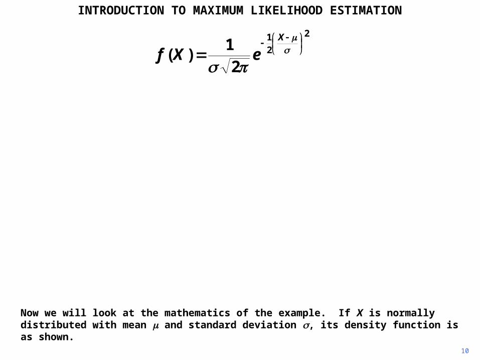
Now we will look at the mathematics of the example. If X is normally distributed with mean and standard deviation , its density function is as shown.
2
21
21
)(
X
eXf
11
INTRODUCTION TO MAXIMUM LIKELIHOOD ESTIMATION
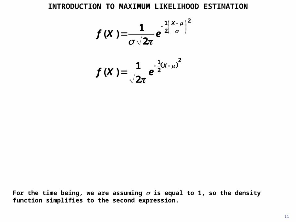
For the time being, we are assuming is equal to 1, so the density function simplifies to the second expression.
2
21
21
)(
X
eXf
2
21
21
)(
X
eXf
12
INTRODUCTION TO MAXIMUM LIKELIHOOD ESTIMATION
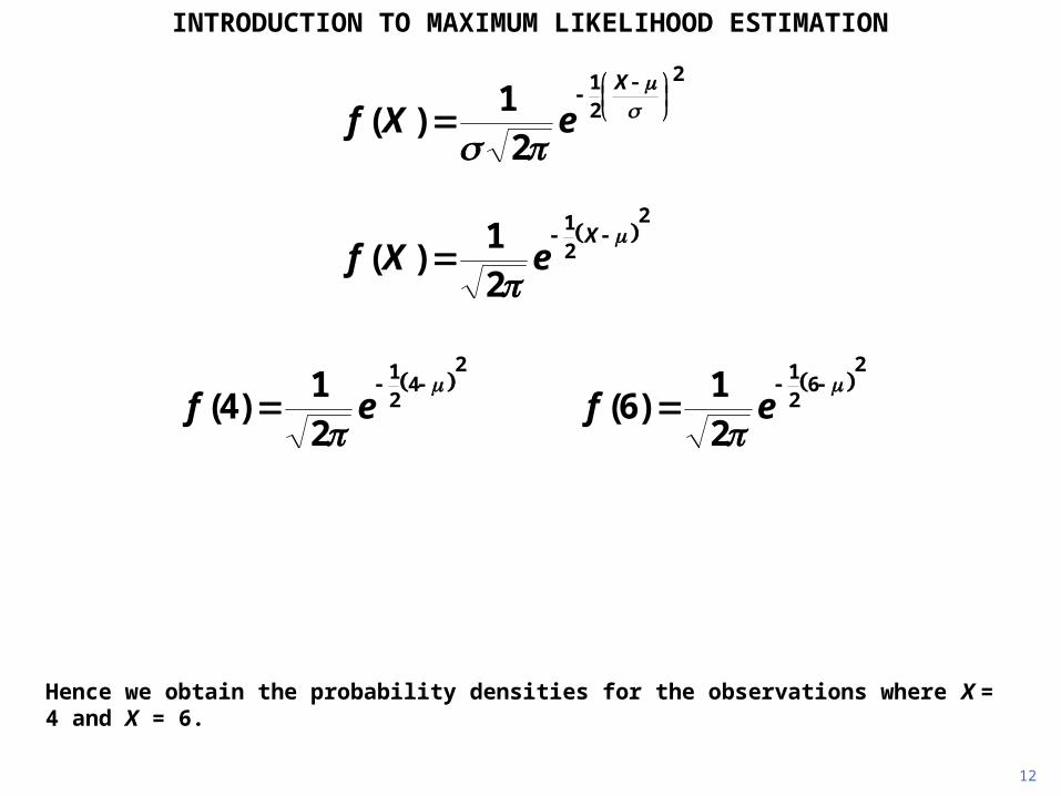
Hence we obtain the probability densities for the observations where X = 4 and X = 6.
2
421
21
)4(
ef
26
21
21
)6(
ef
2
21
21
)(
X
eXf
2
21
21
)(
X
eXf
13
INTRODUCTION TO MAXIMUM LIKELIHOOD ESTIMATION
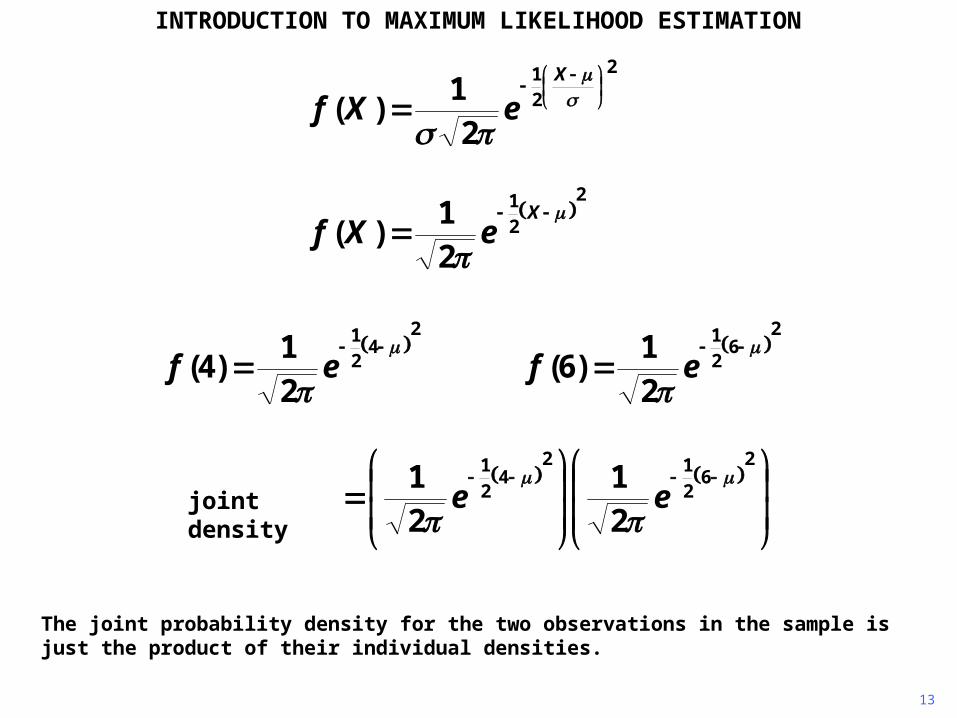
The joint probability density for the two observations in the sample is just the product of their individual densities.
2
421
21
)4(
ef
26
21
21
)6(
ef
2
21
21
)(
X
eXf
2
21
21
)(
X
eXf
2
62
124
2
1
21
21
eejoint density
14
INTRODUCTION TO MAXIMUM LIKELIHOOD ESTIMATION
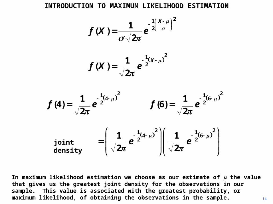
In maximum likelihood estimation we choose as our estimate of the value that gives us the greatest joint density for the observations in our sample. This value is associated with the greatest probability, or maximum likelihood, of obtaining the observations in the sample.
2
21
21
)(
X
eXf
2
21
21
)(
X
eXf
2
421
21
)4(
ef
26
21
21
)6(
ef
2
62
124
2
1
21
21
eejoint density
15
INTRODUCTION TO MAXIMUM LIKELIHOOD ESTIMATION
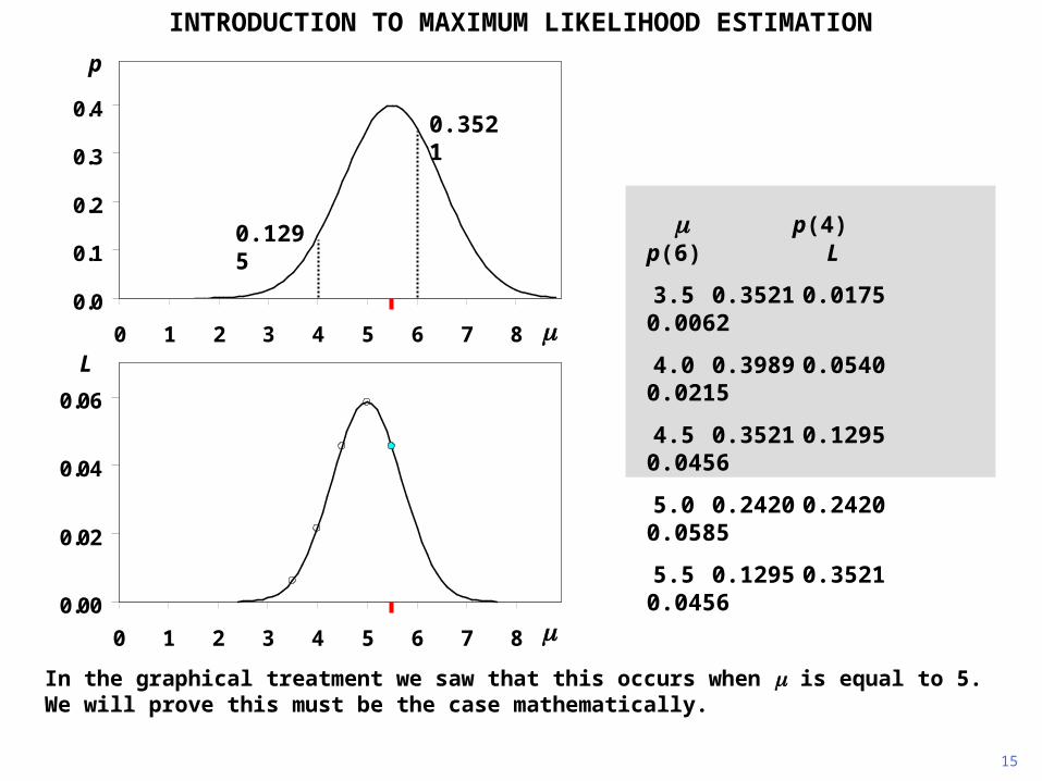
In the graphical treatment we saw that this occurs when is equal to 5. We will prove this must be the case mathematically.
p(4) p(6) L
3.5 0.3521 0.0175 0.0062
4.0 0.3989 0.0540 0.0215
4.5 0.3521 0.1295 0.0456
5.0 0.2420 0.2420 0.0585
5.5 0.1295 0.3521 0.0456
0.00
0.02
0.04
0.06
0 1 2 3 4 5 6 7 8
0.0
0.1
0.2
0.3
0.4
0 1 2 3 4 5 6 7 8
p
L
0.1295
0.3521
16
INTRODUCTION TO MAXIMUM LIKELIHOOD ESTIMATION
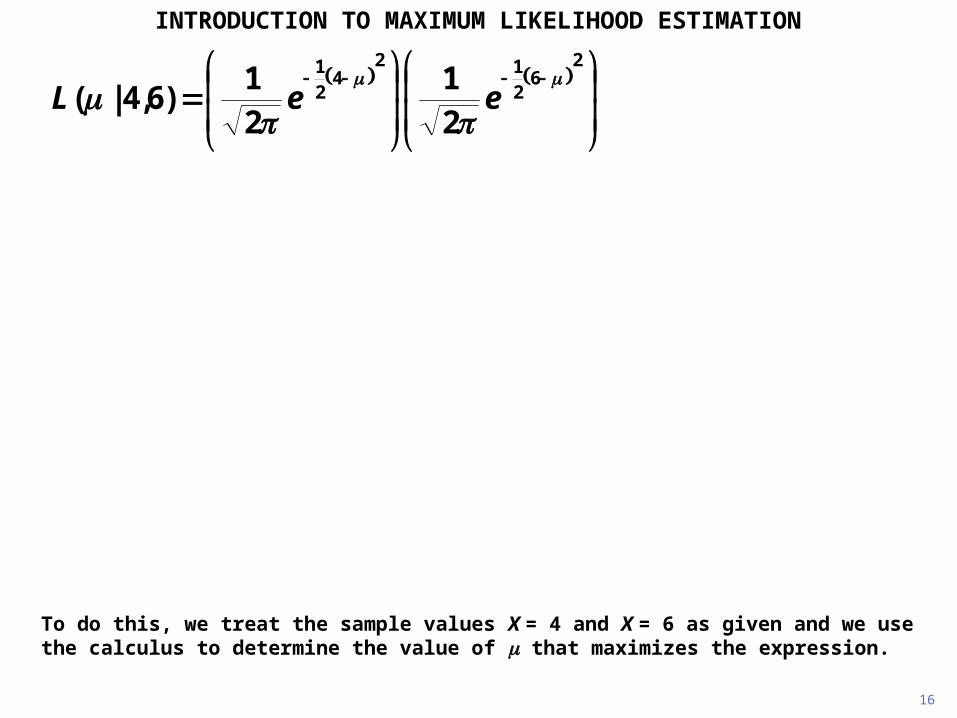
To do this, we treat the sample values X = 4 and X = 6 as given and we use the calculus to determine the value of that maximizes the expression.
2
6212
421
21
21
)6,4|(
eeL
17
INTRODUCTION TO MAXIMUM LIKELIHOOD ESTIMATION
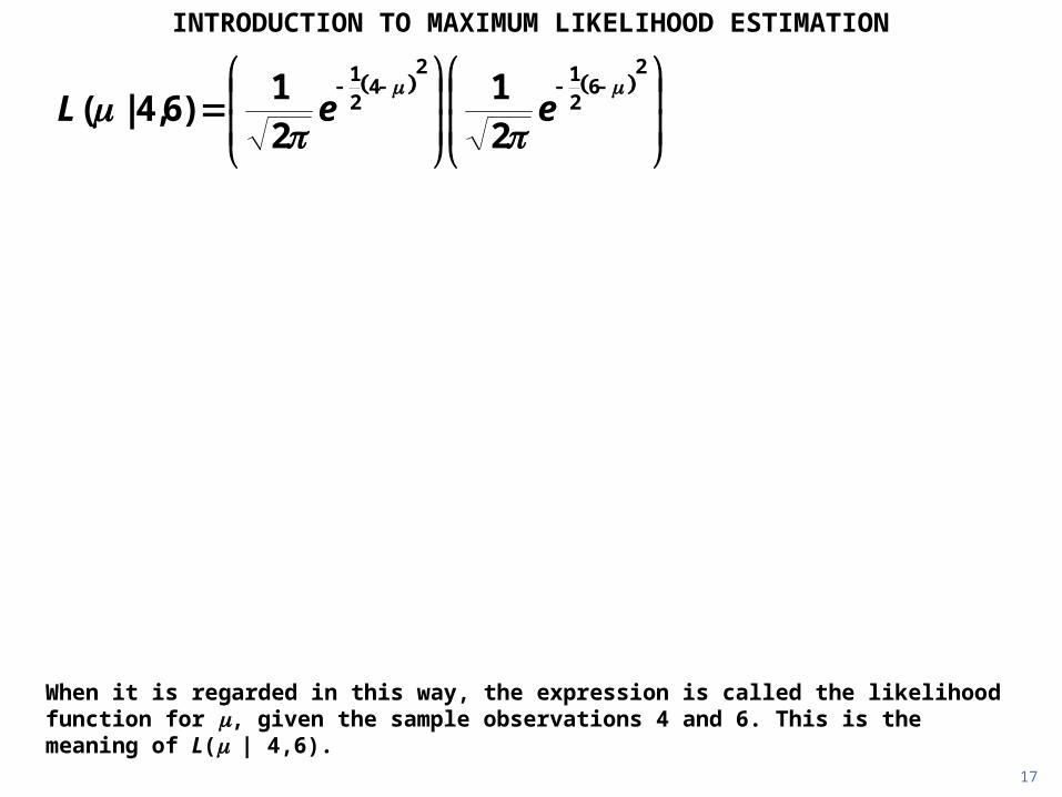
When it is regarded in this way, the expression is called the likelihood function for , given the sample observations 4 and 6. This is the meaning of L(| 4,6).
2
6212
421
21
21
)6,4|(
eeL
18
INTRODUCTION TO MAXIMUM LIKELIHOOD ESTIMATION
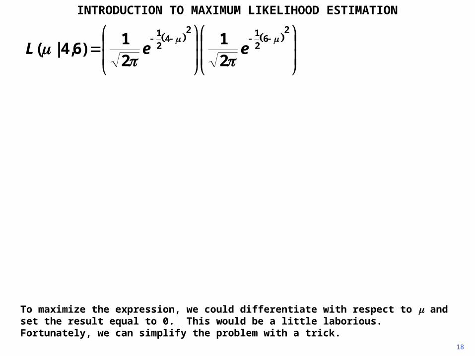
To maximize the expression, we could differentiate with respect to and set the result equal to 0. This would be a little laborious. Fortunately, we can simplify the problem with a trick.
2
6212
421
21
21
)6,4|(
eeL
19
INTRODUCTION TO MAXIMUM LIKELIHOOD ESTIMATION
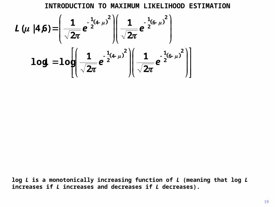
log L is a monotonically increasing function of L (meaning that log L increases if L increases and decreases if L decreases).
2
6212
421
21
21
)6,4|(
eeL
22
26
212
421
26
212
421
26
212
421
621
421
21
log2
log21
loglog21
log
21
log21
log
21
21
loglog
ee
ee
eeL
20
INTRODUCTION TO MAXIMUM LIKELIHOOD ESTIMATION
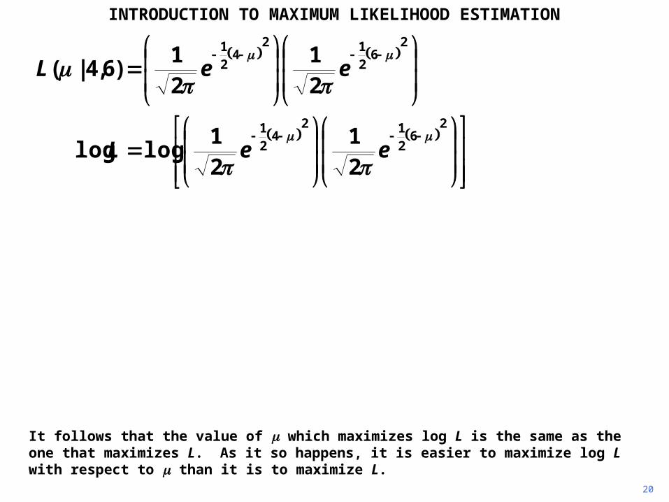
It follows that the value of which maximizes log L is the same as the one that maximizes L. As it so happens, it is easier to maximize log L with respect to than it is to maximize L.
2
6212
421
21
21
)6,4|(
eeL
22
26
212
421
26
212
421
26
212
421
621
421
21
log2
log21
loglog21
log
21
log21
log
21
21
loglog
ee
ee
eeL
21
INTRODUCTION TO MAXIMUM LIKELIHOOD ESTIMATION
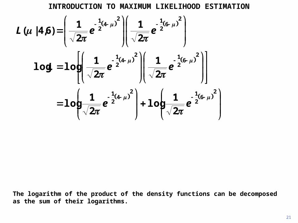
The logarithm of the product of the density functions can be decomposed as the sum of their logarithms.
2
6212
421
21
21
)6,4|(
eeL
22
26
212
421
26
212
421
26
212
421
621
421
21
log2
log21
loglog21
log
21
log21
log
21
21
loglog
ee
ee
eeL
22
INTRODUCTION TO MAXIMUM LIKELIHOOD ESTIMATION
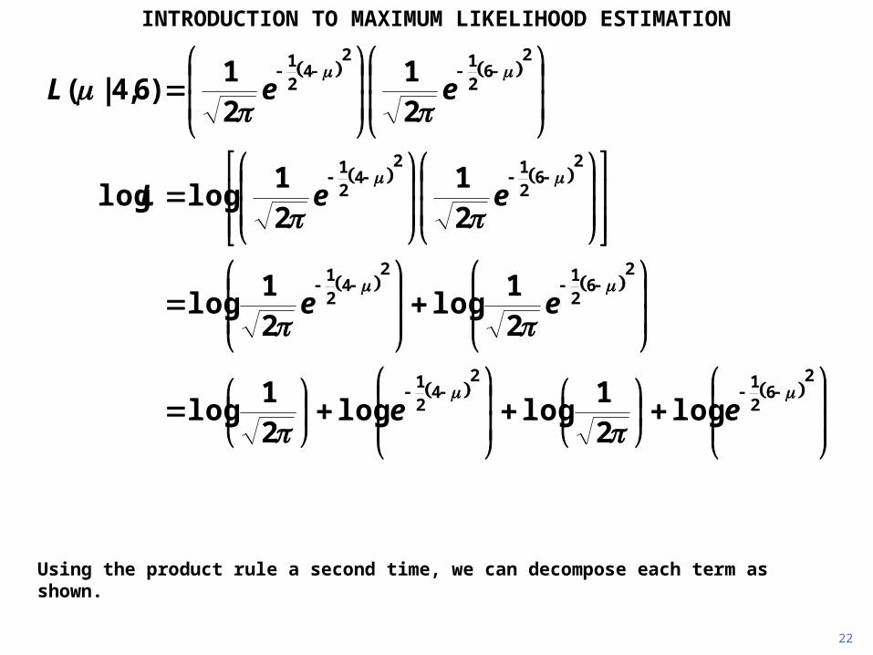
Using the product rule a second time, we can decompose each term as shown.
2
6212
421
21
21
)6,4|(
eeL
22
26
212
421
26
212
421
26
212
421
621
421
21
log2
log21
loglog21
log
21
log21
log
21
21
loglog
ee
ee
eeL
23
INTRODUCTION TO MAXIMUM LIKELIHOOD ESTIMATION
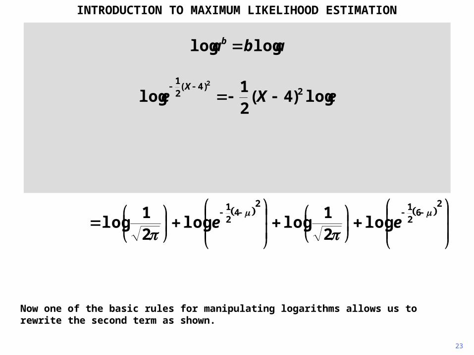
Now one of the basic rules for manipulating logarithms allows us to rewrite the second term as shown.
2
6212
421
21
21
)6,4|(
eeL
22
26
212
421
26
212
421
26
212
421
621
421
21
log2
log21
loglog21
log
21
log21
log
21
21
loglog
ee
ee
eeL
abab loglog
2
2)4(21
)4(21
log)4(21
log2
X
eXeX

24
INTRODUCTION TO MAXIMUM LIKELIHOOD ESTIMATION
log e is equal to 1, another basic logarithm result. (Remember, as always, we are using natural logarithms, that is, logarithms to base e.)
2
6212
421
21
21
)6,4|(
eeL
22
26
212
421
26
212
421
26
212
421
621
421
21
log2
log21
loglog21
log
21
log21
log
21
21
loglog
ee
ee
eeL
abab loglog
2
2)4(21
)4(21
log)4(21
log2
X
eXeX
25
INTRODUCTION TO MAXIMUM LIKELIHOOD ESTIMATION
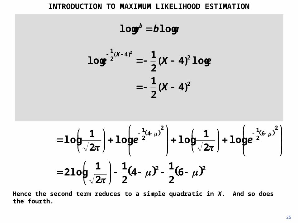
Hence the second term reduces to a simple quadratic in X. And so does the fourth.
2
6212
421
21
21
)6,4|(
eeL
22
26
212
421
26
212
421
26
212
421
621
421
21
log2
log21
loglog21
log
21
log21
log
21
21
loglog
ee
ee
eeL
abab loglog
2
2)4(21
)4(21
log)4(21
log2
X
eXeX
26
INTRODUCTION TO MAXIMUM LIKELIHOOD ESTIMATION
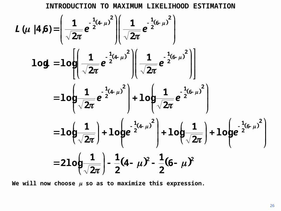
We will now choose so as to maximize this expression.
2
6212
421
21
21
)6,4|(
eeL
22
26
212
421
26
212
421
26
212
421
621
421
21
log2
log21
loglog21
log
21
log21
log
21
21
loglog
ee
ee
eeL
27
INTRODUCTION TO MAXIMUM LIKELIHOOD ESTIMATION
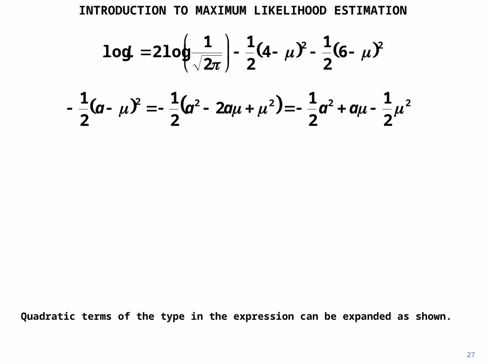
Quadratic terms of the type in the expression can be expanded as shown.
22 621
421
21
log2log
L
22222
21
21
221
21 aaaaa
28
INTRODUCTION TO MAXIMUM LIKELIHOOD ESTIMATION
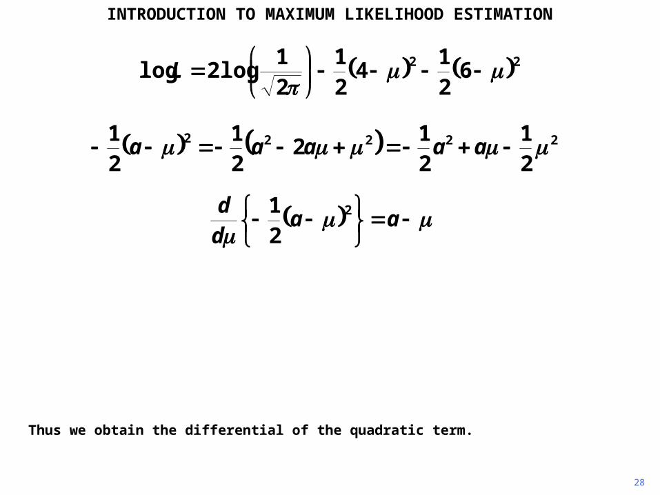
Thus we obtain the differential of the quadratic term.
22 621
421
21
log2log
L
22222
21
21
221
21 aaaaa
aa
dd 2
21
29
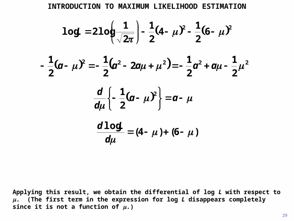
INTRODUCTION TO MAXIMUM LIKELIHOOD ESTIMATION
Applying this result, we obtain the differential of log L with respect to . (The first term in the expression for log L disappears completely since it is not a function of .)
22 621
421
21
log2log
L
22222
21
21
221
21 aaaaa
aa
dd 2
21
)6()4(log
dLd
30
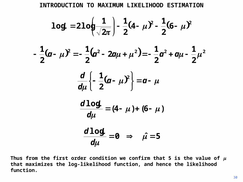
INTRODUCTION TO MAXIMUM LIKELIHOOD ESTIMATION
Thus from the first order condition we confirm that 5 is the value of that maximizes the log-likelihood function, and hence the likelihood function.
22 621
421
21
log2log
L
22222
21
21
221
21 aaaaa
aa
dd 2
21
)6()4(log
dLd
5ˆ0log
dLd
31
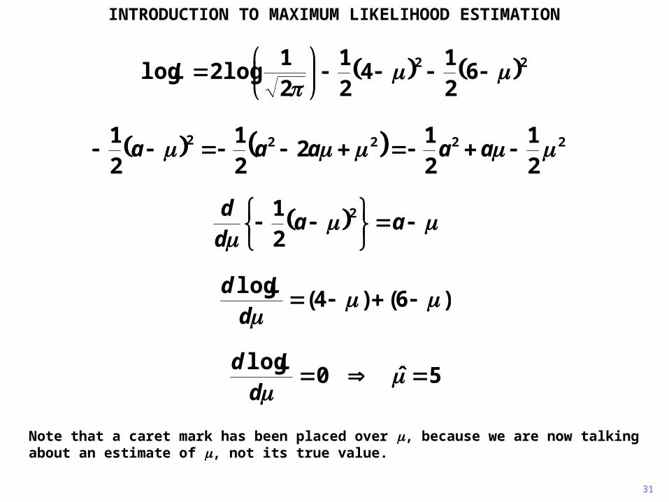
INTRODUCTION TO MAXIMUM LIKELIHOOD ESTIMATION
Note that a caret mark has been placed over , because we are now talking about an estimate of , not its true value.
22 621
421
21
log2log
L
22222
21
21
221
21 aaaaa
aa
dd 2
21
)6()4(log
dLd
5ˆ0log
dLd
32
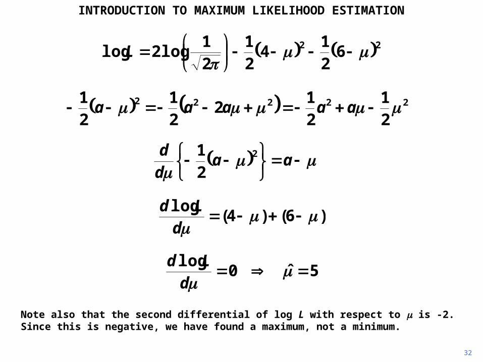
INTRODUCTION TO MAXIMUM LIKELIHOOD ESTIMATION
Note also that the second differential of log L with respect to is -2. Since this is negative, we have found a maximum, not a minimum.
22 621
421
21
log2log
L
22222
21
21
221
21 aaaaa
aa
dd 2
21
)6()4(log
dLd
5ˆ0log
dLd
33
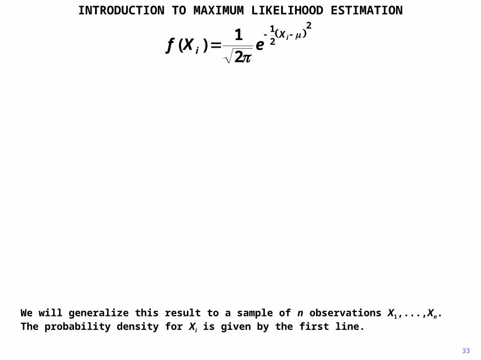
INTRODUCTION TO MAXIMUM LIKELIHOOD ESTIMATION
We will generalize this result to a sample of n observations X1,...,Xn. The probability density for Xi is given by the first line.
2
21
21
)(
iX
i eXf
34
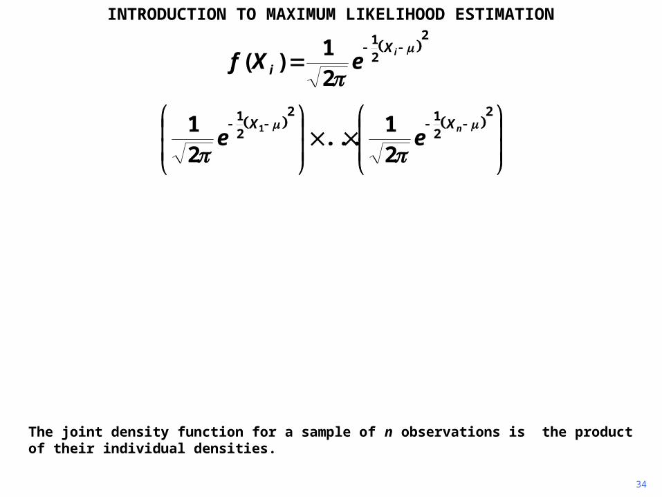
INTRODUCTION TO MAXIMUM LIKELIHOOD ESTIMATION
The joint density function for a sample of n observations is the product of their individual densities.
2
212
21
21
...21 1
nXX
ee
2
21
21
)(
iX
i eXf
35
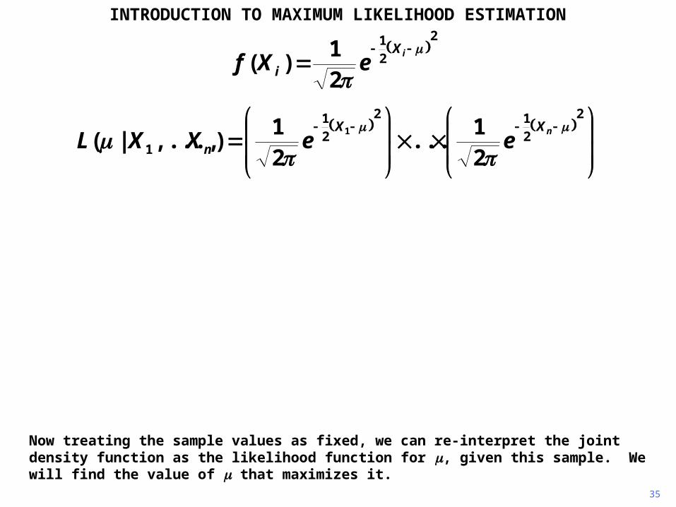
INTRODUCTION TO MAXIMUM LIKELIHOOD ESTIMATION
Now treating the sample values as fixed, we can re-interpret the joint density function as the likelihood function for , given this sample. We will find the value of that maximizes it.
2
21
21
)(
iX
i eXf
2
212
21
1 21
...21
),...,|(1
nXX
n eeXXL
36
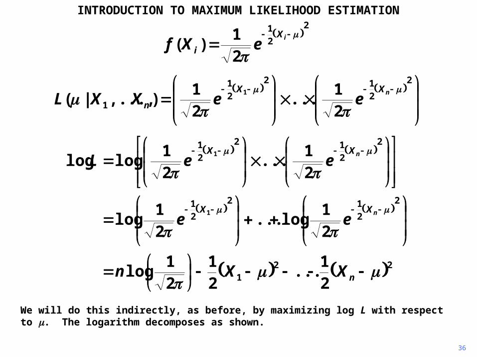
INTRODUCTION TO MAXIMUM LIKELIHOOD ESTIMATION
We will do this indirectly, as before, by maximizing log L with respect to . The logarithm decomposes as shown.
2
212
21
1 21
...21
),...,|(1
nXX
n eeXXL
221
2
212
21
2
212
21
21
...21
21
log
21
log...21
log
21
...21
loglog
1
1
n
XX
XX
XXn
ee
eeL
n
n
2
21
21
)(
iX
i eXf
37
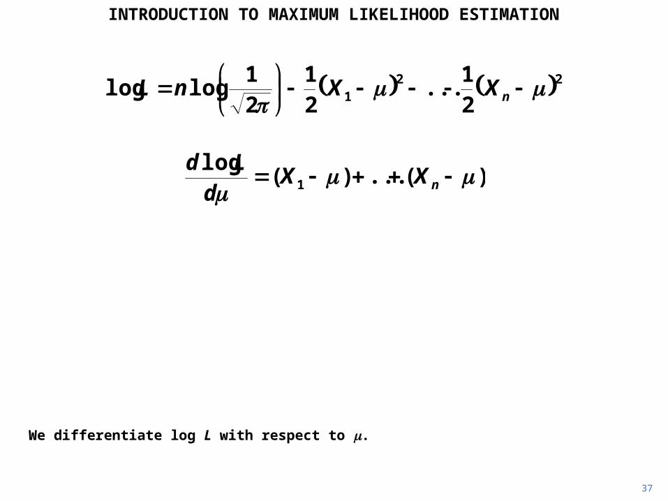
INTRODUCTION TO MAXIMUM LIKELIHOOD ESTIMATION
We differentiate log L with respect to .
)(...)(log
1
nXXdLd
221 2
1...
21
21
loglog
nXXnL

38
INTRODUCTION TO MAXIMUM LIKELIHOOD ESTIMATION
The first order condition for a minimum is that the differential be equal to zero.
0ˆ0log
nX
dLd
i
)(...)(log
1
nXXdLd
221 2
1...
21
21
loglog
nXXnL
39
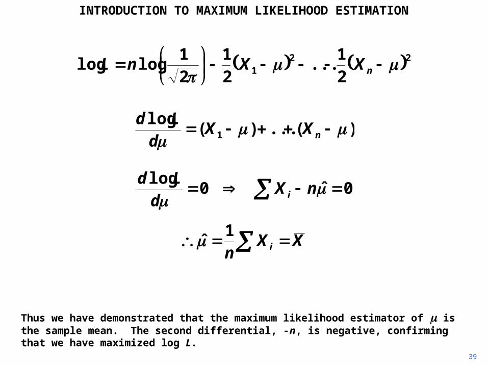
INTRODUCTION TO MAXIMUM LIKELIHOOD ESTIMATION
Thus we have demonstrated that the maximum likelihood estimator of is the sample mean. The second differential, -n, is negative, confirming that we have maximized log L.
221 2
1...
21
21
loglog
nXXnL
)(...)(log
1
nXXdLd
0ˆ0log
nX
dLd
i
XXn i
1̂
40
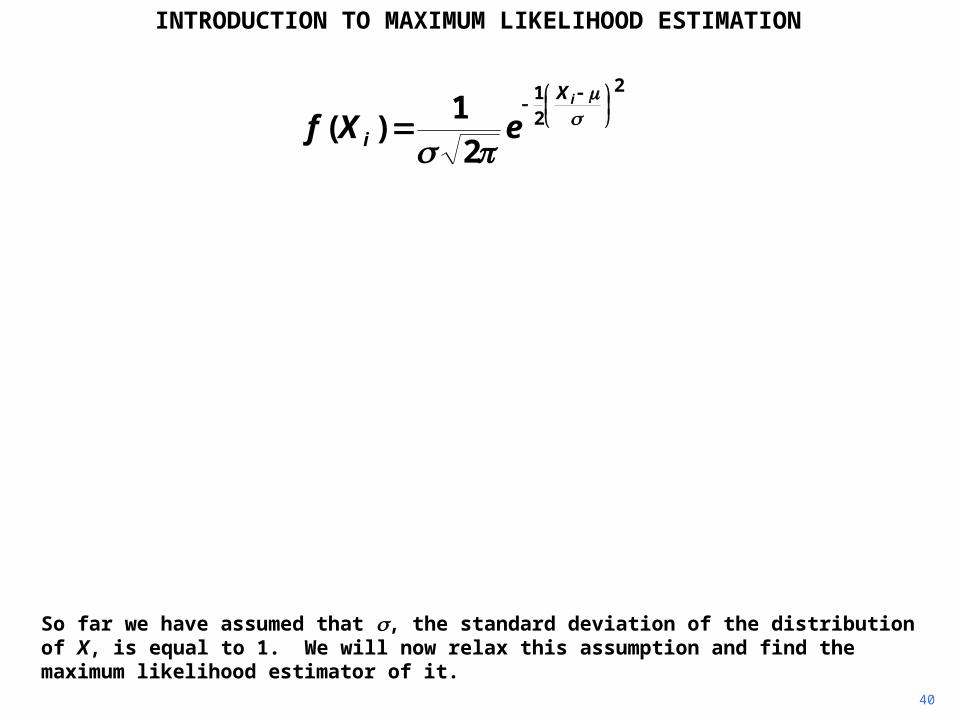
INTRODUCTION TO MAXIMUM LIKELIHOOD ESTIMATION
So far we have assumed that , the standard deviation of the distribution of X, is equal to 1. We will now relax this assumption and find the maximum likelihood estimator of it.
2
21
21
)(
iX
i eXf

41
INTRODUCTION TO MAXIMUM LIKELIHOOD ESTIMATION
We will illustrate the process graphically with the two-observation example, keeping fixed at 5. We will start with equal to 2.
0.0
0.2
0.4
0.6
0.8
0 1 2 3 4 5 6 7 8 9
L
p
0
0.02
0.04
0.06
0 1 2 3 4
42
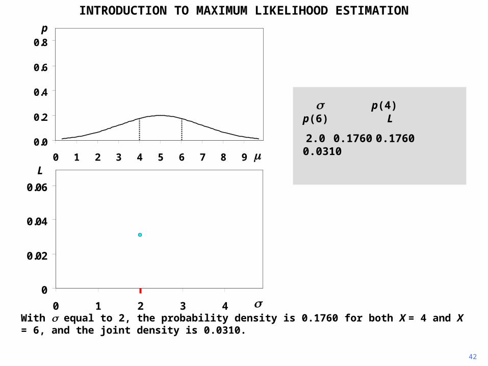
INTRODUCTION TO MAXIMUM LIKELIHOOD ESTIMATION
With equal to 2, the probability density is 0.1760 for both X = 4 and X = 6, and the joint density is 0.0310.
0.0
0.2
0.4
0.6
0.8
0 1 2 3 4 5 6 7 8 9
L
p
p(4) p(6) L
2.0 0.1760 0.1760 0.0310
0
0.02
0.04
0.06
0 1 2 3 4
43
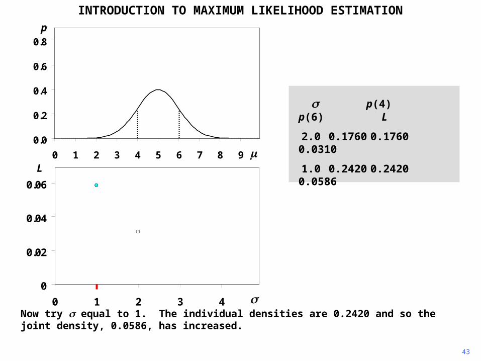
INTRODUCTION TO MAXIMUM LIKELIHOOD ESTIMATION
Now try equal to 1. The individual densities are 0.2420 and so the joint density, 0.0586, has increased.
0.0
0.2
0.4
0.6
0.8
0 1 2 3 4 5 6 7 8 9
L
p
p(4) p(6) L
2.0 0.1760 0.1760 0.0310
1.0 0.2420 0.2420 0.0586
0
0.02
0.04
0.06
0 1 2 3 4
44
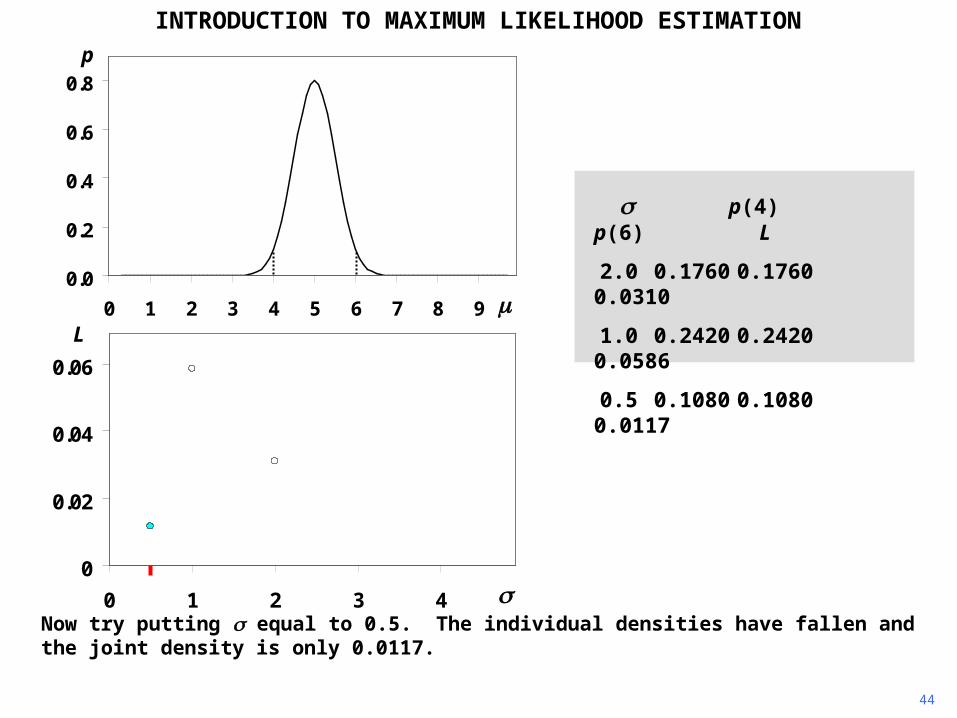
INTRODUCTION TO MAXIMUM LIKELIHOOD ESTIMATION
Now try putting equal to 0.5. The individual densities have fallen and the joint density is only 0.0117.
0.0
0.2
0.4
0.6
0.8
0 1 2 3 4 5 6 7 8 9
L
p
p(4) p(6) L
2.0 0.1760 0.1760 0.0310
1.0 0.2420 0.2420 0.0586
0.5 0.1080 0.1080 0.0117
0
0.02
0.04
0.06
0 1 2 3 4
45
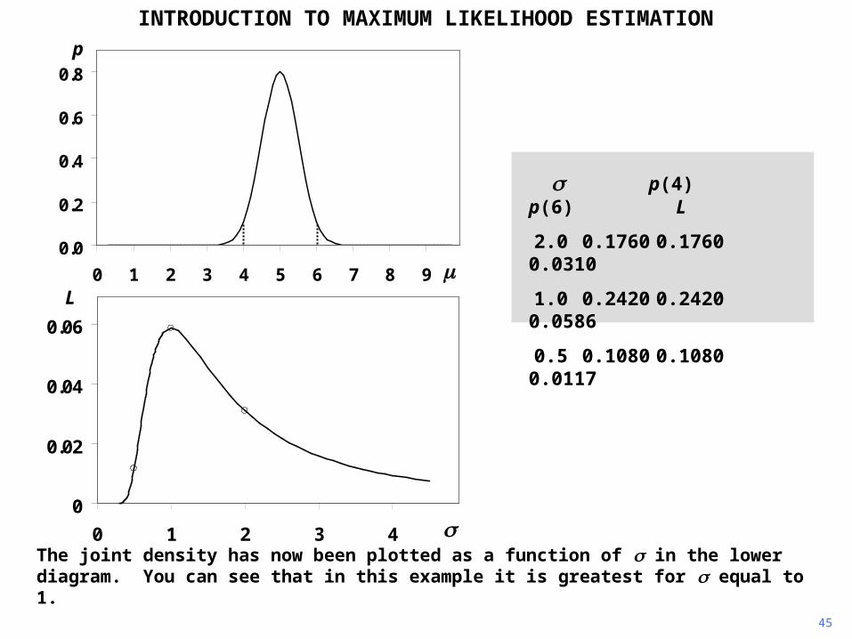
INTRODUCTION TO MAXIMUM LIKELIHOOD ESTIMATION
The joint density has now been plotted as a function of in the lower diagram. You can see that in this example it is greatest for equal to 1.
0
0.02
0.04
0.06
0 1 2 3 4
0.0
0.2
0.4
0.6
0.8
0 1 2 3 4 5 6 7 8 9
p(4) p(6) L
2.0 0.1760 0.1760 0.0310
1.0 0.2420 0.2420 0.0586
0.5 0.1080 0.1080 0.0117L
p
46
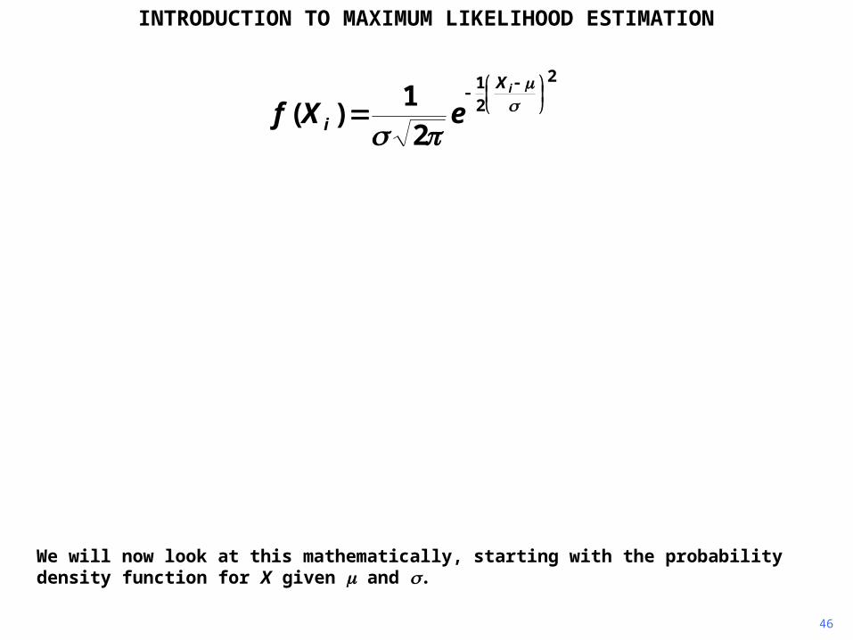
INTRODUCTION TO MAXIMUM LIKELIHOOD ESTIMATION
We will now look at this mathematically, starting with the probability density function for X given and .
2
21
21
)(
iX
i eXf
47
INTRODUCTION TO MAXIMUM LIKELIHOOD ESTIMATION
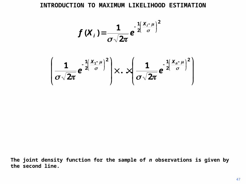
The joint density function for the sample of n observations is given by the second line.
2
21
21
)(
iX
i eXf
2
212
21
21
...21 1
nXX
ee

48
INTRODUCTION TO MAXIMUM LIKELIHOOD ESTIMATION
As before, we can re-interpret this function as the likelihood function for and , given the sample of observations.
2
21
21
)(
iX
i eXf
2
212
21
1 21
...21
),...,|,(1
nXX
n eeXXL
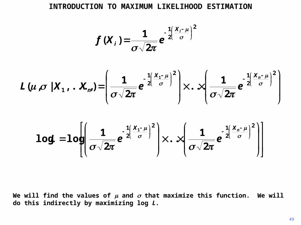
49
INTRODUCTION TO MAXIMUM LIKELIHOOD ESTIMATION
We will find the values of and that maximize this function. We will do this indirectly by maximizing log L.
2
21
21
)(
iX
i eXf
2
212
21
21
...21
loglog1
nXX
eeL
2
212
21
1 21
...21
),...,|,(1
nXX
n eeXXL
50
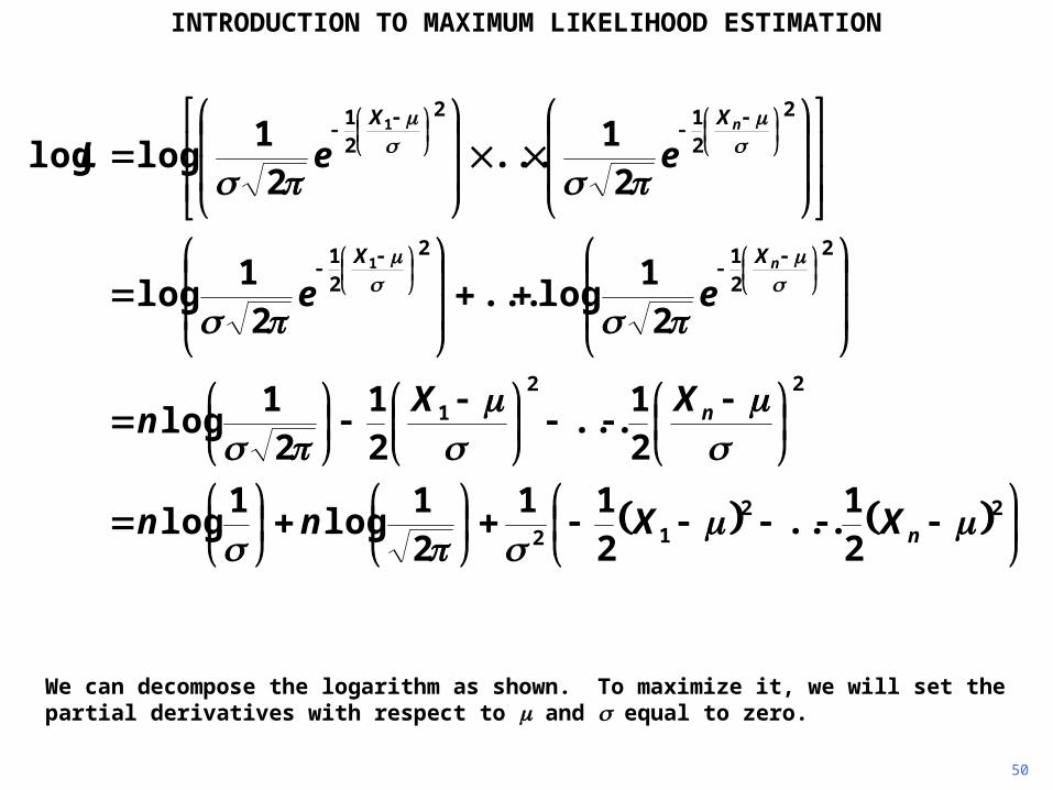
INTRODUCTION TO MAXIMUM LIKELIHOOD ESTIMATION
We can decompose the logarithm as shown. To maximize it, we will set the partial derivatives with respect to and equal to zero.
2212
22
1
2
212
21
2
212
21
21
...211
21
log1
log
21
...21
21
log
21
log...21
log
21
...21
loglog
1
1
n
n
XX
XX
XXnn
XXn
ee
eeL
n
n
51
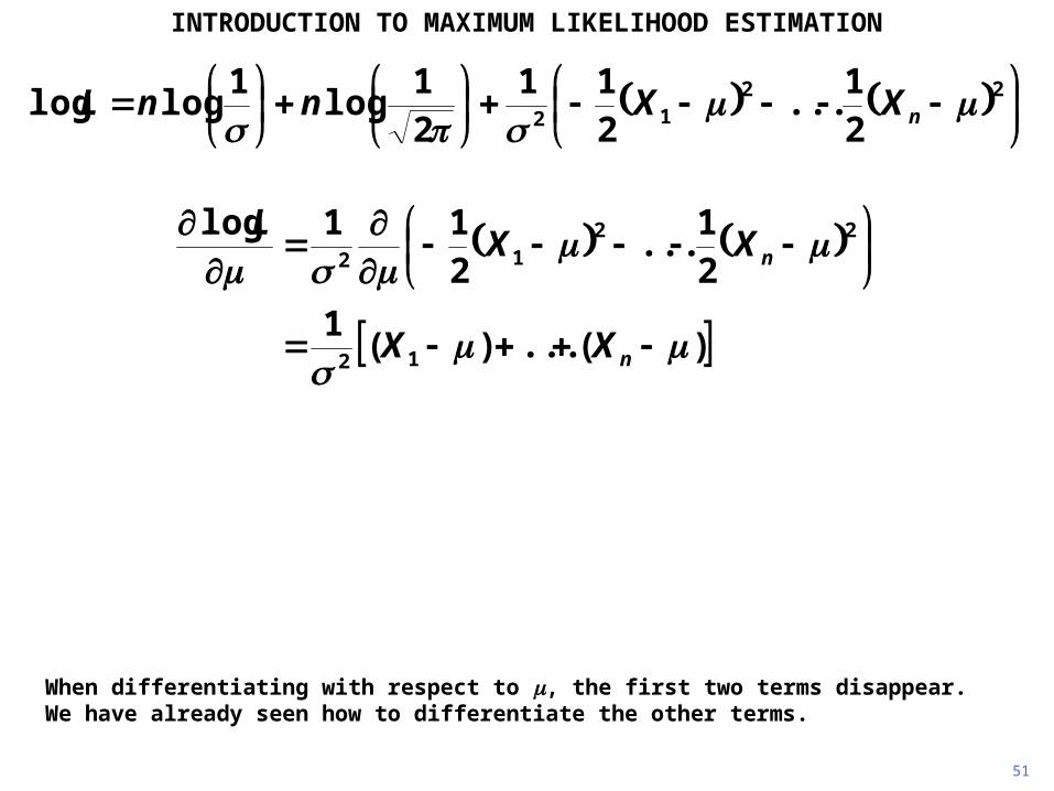
INTRODUCTION TO MAXIMUM LIKELIHOOD ESTIMATION
When differentiating with respect to , the first two terms disappear. We have already seen how to differentiate the other terms.
2
2
2212
221
loglog
21
...211
21
log1
loglog
i
n
Xnn
XXnnL
nX
XX
XXL
i
n
n
2
12
2212
1
)(...)(1
21
...211log
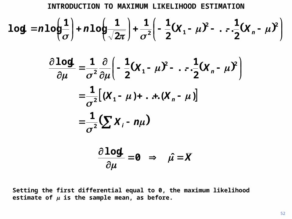
52
INTRODUCTION TO MAXIMUM LIKELIHOOD ESTIMATION
Setting the first differential equal to 0, the maximum likelihood estimate of is the sample mean, as before.
XL
ˆ0
log
2
2
2212
221
loglog
21
...211
21
log1
loglog
i
n
Xnn
XXnnL
nX
XX
XXL
i
n
n
2
12
2212
1
)(...)(1
21
...211log
53
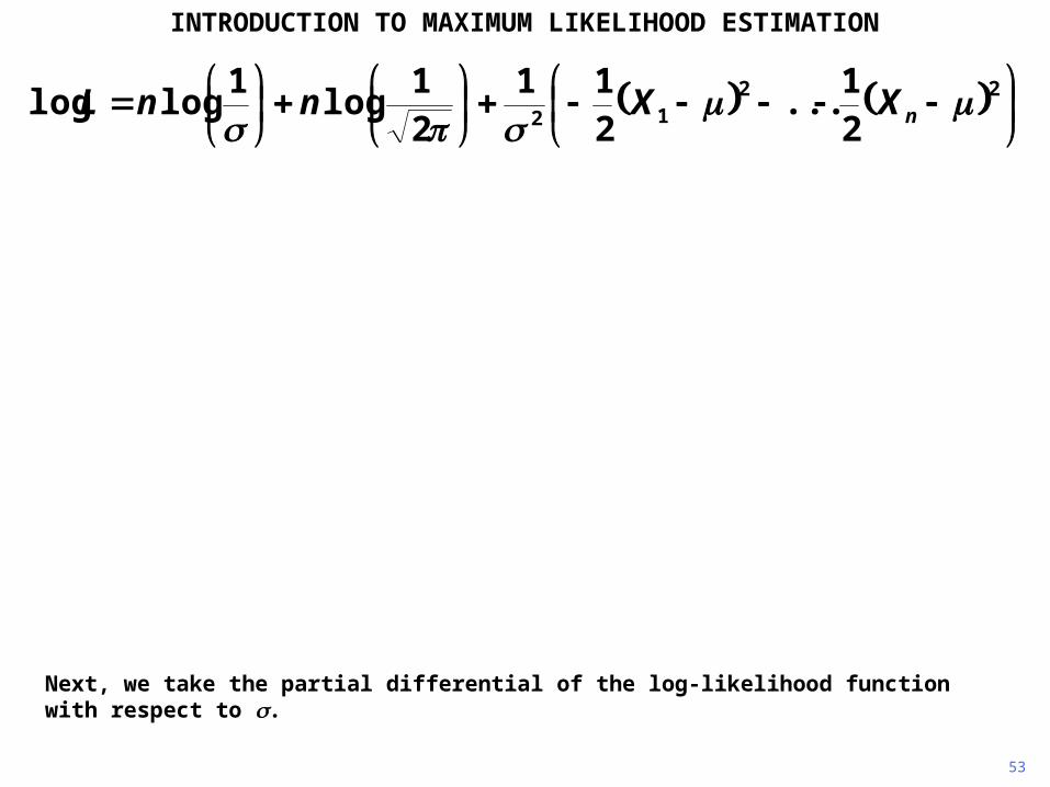
INTRODUCTION TO MAXIMUM LIKELIHOOD ESTIMATION
Next, we take the partial differential of the log-likelihood function with respect to .
2
2
2212
221
loglog
21
...211
21
log1
loglog
i
n
Xnn
XXnnL
54
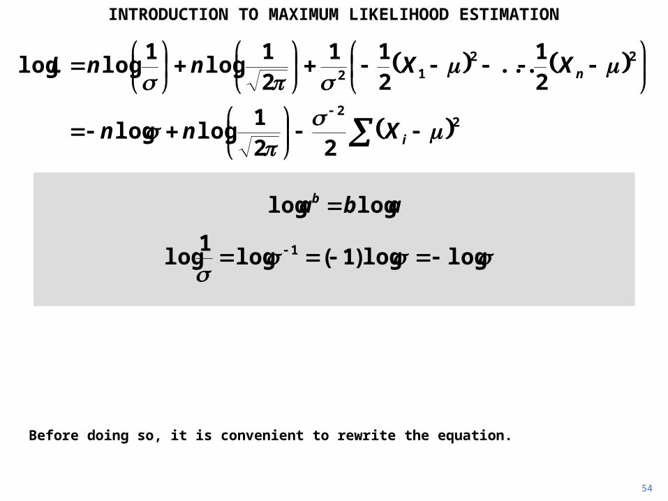
INTRODUCTION TO MAXIMUM LIKELIHOOD ESTIMATION
Before doing so, it is convenient to rewrite the equation.
abab loglog
loglog)1(log1
log 1
2
2
2212
221
loglog
21
...211
21
log1
loglog
i
n
Xnn
XXnnL
55
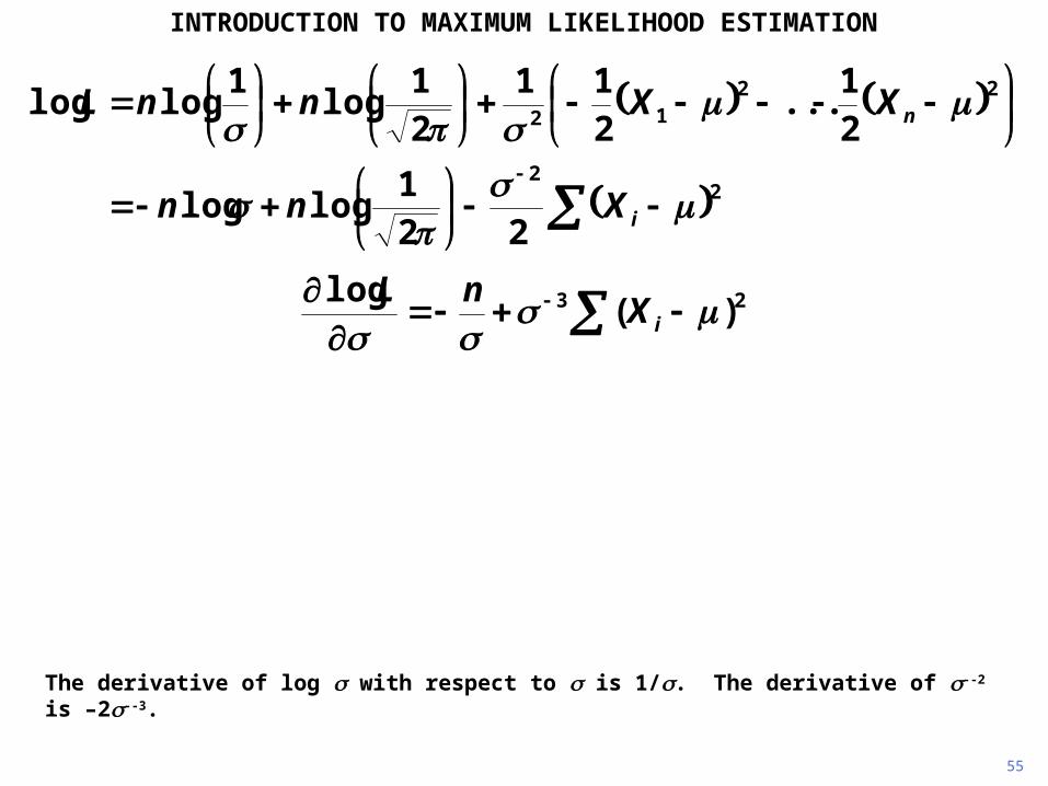
INTRODUCTION TO MAXIMUM LIKELIHOOD ESTIMATION
The derivative of log with respect to is 1/. The derivative of --2 is –2--3.
23 )(log
iXnL
2
2
2212
221
loglog
21
...211
21
log1
loglog
i
n
Xnn
XXnnL
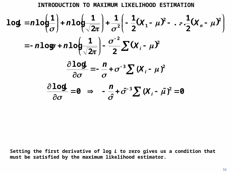
56
INTRODUCTION TO MAXIMUM LIKELIHOOD ESTIMATION
Setting the first derivative of log L to zero gives us a condition that must be satisfied by the maximum likelihood estimator.
0)ˆ(ˆˆ
0log 23
iXnL
23 )(log
iXnL
2
2
2212
221
loglog
21
...211
21
log1
loglog
i
n
Xnn
XXnnL
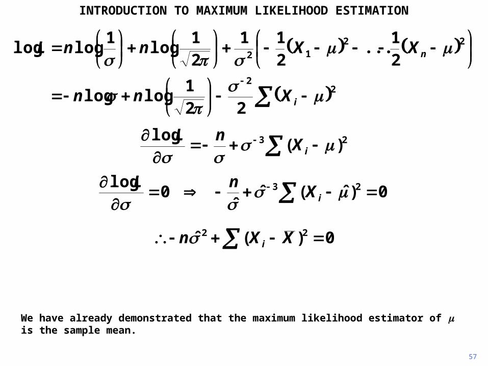
57
INTRODUCTION TO MAXIMUM LIKELIHOOD ESTIMATION
We have already demonstrated that the maximum likelihood estimator of is the sample mean.
0)(ˆ 22 XXn i
0)ˆ(ˆˆ
0log 23
iXnL
23 )(log
iXnL
2
2
2212
221
loglog
21
...211
21
log1
loglog
i
n
Xnn
XXnnL
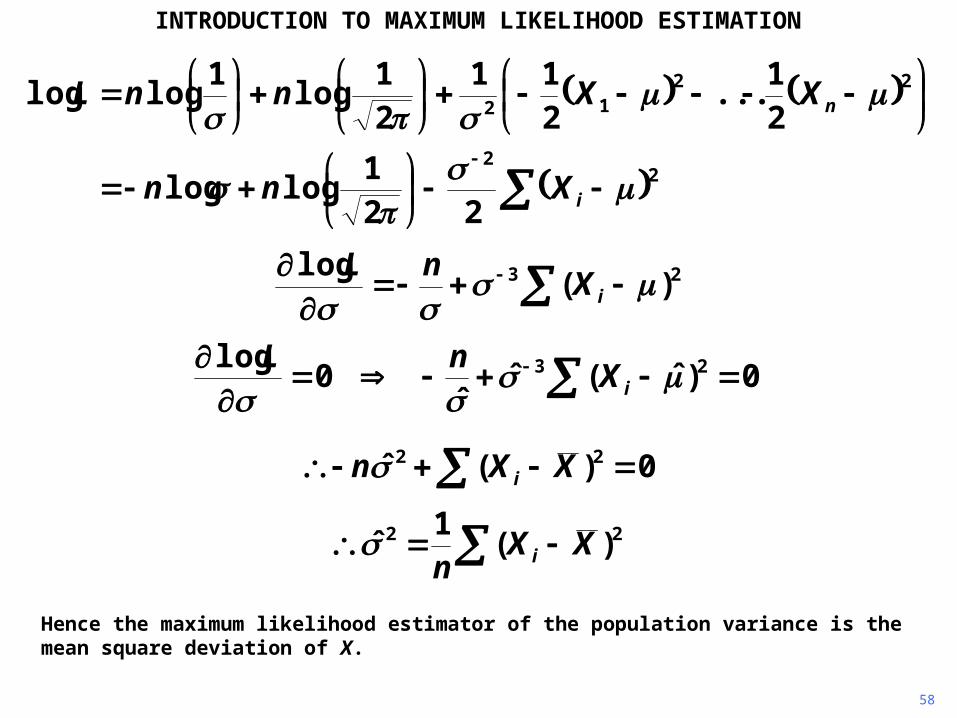
58
INTRODUCTION TO MAXIMUM LIKELIHOOD ESTIMATION
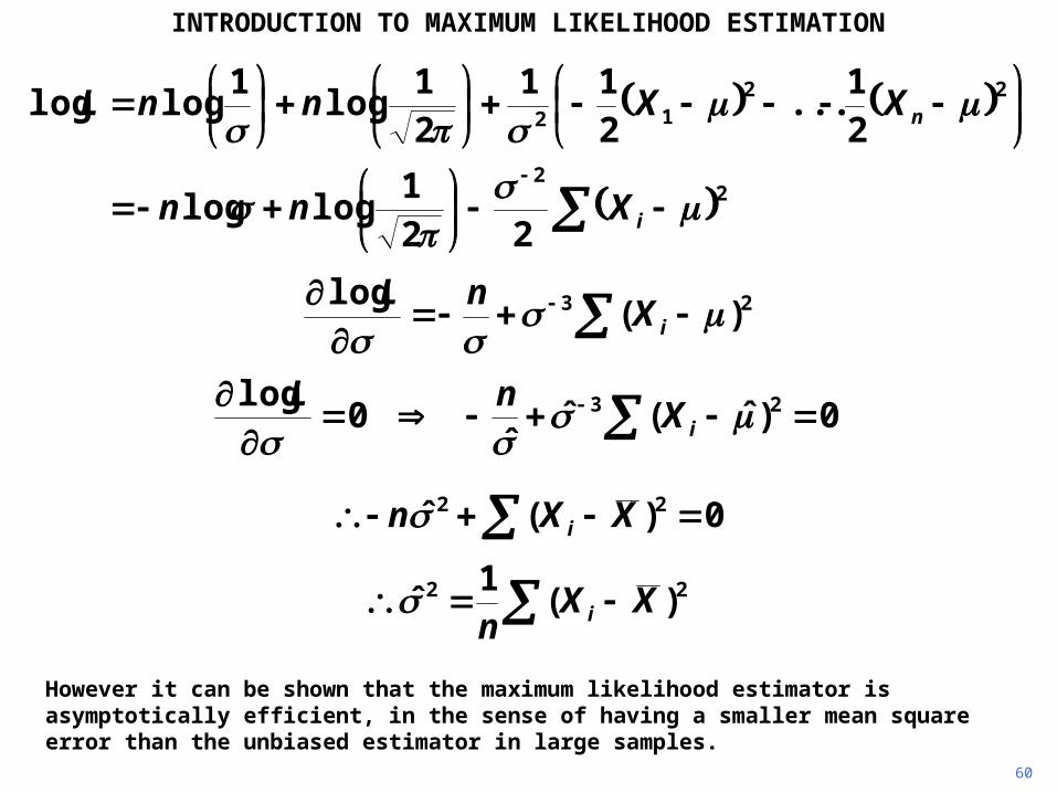
Hence the maximum likelihood estimator of the population variance is the mean square deviation of X.
22 )(1
ˆ XXn i
0)(ˆ 22 XXn i
0)ˆ(ˆˆ
0log 23
iXnL
23 )(log
iXnL
2
2
2212
221
loglog
21
...211
21
log1
loglog
i
n
Xnn
XXnnL
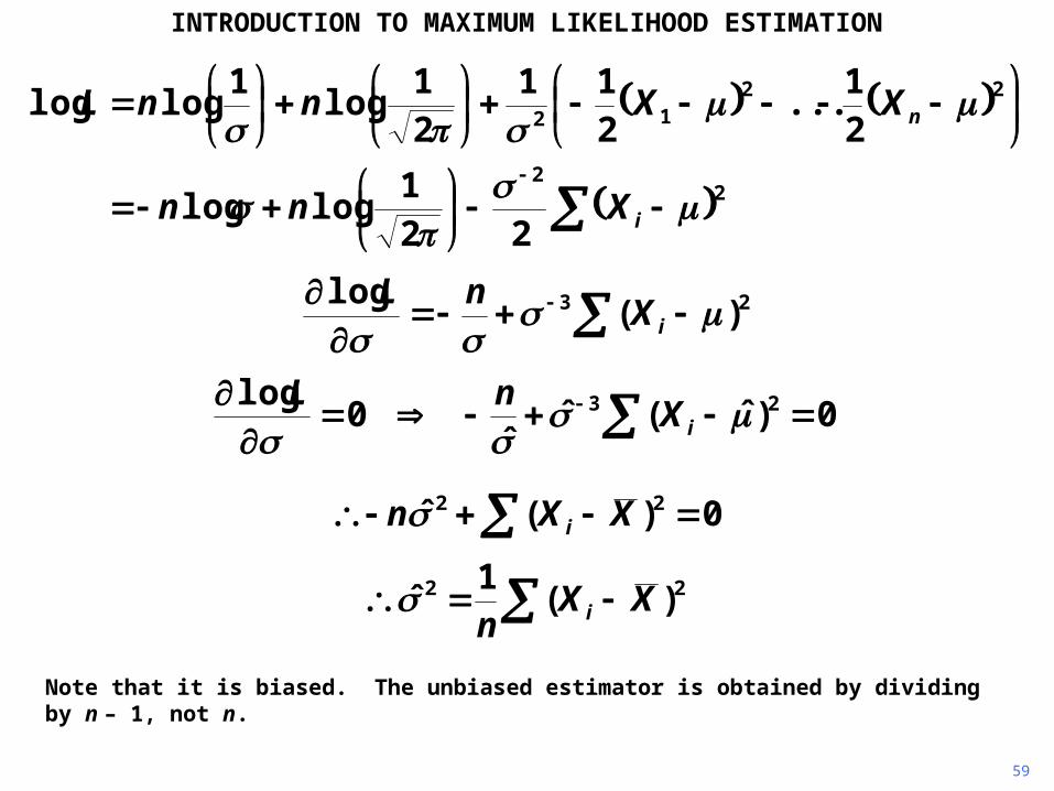
59
INTRODUCTION TO MAXIMUM LIKELIHOOD ESTIMATION
Note that it is biased. The unbiased estimator is obtained by dividing by n – 1, not n.
23 )(log
iXnL
2
2
2212
221
loglog
21
...211
21
log1
loglog
i
n
Xnn
XXnnL
0)ˆ(ˆˆ
0log 23
iXnL
0)(ˆ 22 XXn i
22 )(1
ˆ XXn i
INTRODUCTION TO MAXIMUM LIKELIHOOD ESTIMATION
23 )(log
iXnL
2
2
2212
221
loglog
21
...211
21
log1
loglog
i
n
Xnn
XXnnL
0)ˆ(ˆˆ
0log 23
iXnL
0)(ˆ 22 XXn i
However it can be shown that the maximum likelihood estimator is asymptotically efficient, in the sense of having a smaller mean square error than the unbiased estimator in large samples.
60
22 )(1
ˆ XXn i

Copyright Christopher Dougherty 2011.
These slideshows may be downloaded by anyone, anywhere for personal use.
Subject to respect for copyright and, where appropriate, attribution, they may be
used as a resource for teaching an econometrics course. There is no need to
refer to the author.
The content of this slideshow comes from Section 10.6 of C. Dougherty,
Introduction to Econometrics, fourth edition 2011, Oxford University Press.
Additional (free) resources for both students and instructors may be
downloaded from the OUP Online Resource Centre
http://www.oup.com/uk/orc/bin/9780199567089/.
Individuals studying econometrics on their own and who feel that they might
benefit from participation in a formal course should consider the London School
of Economics summer school course
EC212 Introduction to Econometrics
http://www2.lse.ac.uk/study/summerSchools/summerSchool/Home.aspx
or the University of London International Programmes distance learning course
20 Elements of Econometrics
www.londoninternational.ac.uk/lse.
11.07.25
Related Documents